Analytic for Data-Driven Decision-Making in

Complex High-Dimensional Time-to-Event Data

A Dissertation Presented

by

Keivan Sadeghzadeh

to

The Department of Mechanical and Industrial Engineering

in partial fulfillment of the requirements

for the degree of

Doctor of Philosophy

in

Industrial Engineering

Northeastern University

Boston, Massachusetts

Aug 2015

c©2015 – Keivan Sadeghzadeh

all rights reserved.

To the best wife, my love

Niloofar,

and to my shining star, my son

Kian.

ii

Acknowledgments

I wish to thank everyone who made this dissertation possible.

I would like to extend my deepest appreciation to my research advisor, Professor Nasser

Fard, for his technical and editorial advice which was essential for bringing this research to

its current form. I am especially grateful for his excellent direction and the enthusiasm he

expressed for my work.

This research greatly benefited from the useful suggestions and comments from the mem-

bers of my exceptional doctoral committee, Professors Vinod Sahney and Tucker Marion.

I wish to thank them for all their contributions.

I want to express my sincere gratitude to my beloved wife, Niloofar Montazeri, for provid-

ing me with motivation, understanding, support and encouragement at every step of this

pursuit.

Many thanks go to Kian as well, the best child a father could have, for giving me the op-

portunity to get this work done. I am extremely grateful for having him and already proud

of him.

iii

Abstract

In the era of big data, analysis of complex and huge data expends time

and money, may cause errors and misinterpretations. Consequently, inac-

curate and erroneous reasoning could lead to poor inference and decision-

making, sometimes irreversible and catastrophic events. On the other hand,

proper management and utilization of valuable data could signicantly in-

crease knowledge and reduce cost by preventive actions. In many areas,

there are great interests in time and causes of events. Time-to-event data

analysis is a kernel of risk assessment and has an inevitable role in pre-

dicting the probability of many events occurrence. In addition, variable se-

lection and classication procedures are an integral part of data analysis

where the information revolution brings larger datasets with more variables

and it has become more dicult to process the streaming high-dimensional

time-to-event data in traditional application approaches, specically in the

occurrence of censored observations. Thus, in the presence of large-scale,

massive and complex data, specically in terms of variables, applying proper

methods to eciently simplify such data is desired. Most of the traditional

variable selection methods involve computational algorithms in a class of non-

deterministic polynomial-time hard (NP-hard) that makes these procedures

infeasible. Although recent methods may operate faster, involve dierent

estimation methods and assumptions, their applications are limited, their

assumptions cause restrictions, their computational complexities are costly,

or their robustness is not consistent.

This research is motivated by the importance of the applied variable re-

duction in complex high-dimensional time-to-event data to avoid aforemen-

tioned diculties in decision-making and facilitate time-to-event data anal-

ysis. Quantitative statistical and computational methodologies using com-

binatorial heuristic algorithms for variable selection and classication are

proposed. The purpose of these methodologies is to reduce the volume of the

explanatory variables and identify a set of most inuential variables in such

datasets.

In Chapter 1, an introduction to this research, problem denition and ap-

proach outline are provided through literature review.

In Chapter 2, comprehensive review of time-to-event data analysis dealing

with censoring, survival and hazard function, and categories of this type

of data is presented. This review is completed with an applied denition of

decision-making process. Next, prominent data analysis tools and techniques

is presented including discretization and randomization processes, and data

reduction methods. Finally accelerated failure time model is introduced and

dened.

Chapter 3 provides Methodology I: Nonparametric Re-sampling Methods for

KaplanMeier Estimator Test. In this methodology, an analytical model for

logical transformation of the explanatory variable dataset is proposed and

a class of hybrid nonparametric variable selection methods and algorithms

through variable ineciency recognition are designed. The experimental re-

sults and comparison of them with well-known methods and simulation pat-

terns are presented next.

Chapter 4 describes Methodology II: Heuristic Randomized Decision-Making

Methods through Accelerated Failure Time Model. The methodology, in-

cluding analytical model for the normal transformation of the explanatory

variable dataset as well as heuristic randomized methods and algorithms are

proposed. Finally, the simulation experiment, result and analysis of variable

selection decision-making algorithms are presented.

In Chapter 5, Methodology III: Hybrid Clustering and Classication Meth-

ods using Normalized Weighted K-Mean is proposed. In this methodology,

two dierent methods in order to cluster and classify variables are designed.

Result and analysis of variable clustering and classication are included as

2

well.

In Chapter 6, concluding remarks, a summary of the proposed methods and

their advantages is presented. In addition, an overview for further studies

will be discussed.

The computer package used in this research is the MATLAB® R2011b pro-

gramming environment.

3

Contents

List of Figures 6

List of Tables 8

1 Introduction 10

1.1 Overview . . . . . . . . . . . . . . . . . . . . . . . . . . . . . . 10

1.2 Literature Review . . . . . . . . . . . . . . . . . . . . . . . . . 12

1.3 Problem Denition and Solution Approach . . . . . . . . . . . 15

1.4 Big Data Analytics . . . . . . . . . . . . . . . . . . . . . . . . 17

1.5 Specialty and Application . . . . . . . . . . . . . . . . . . . . 20

1.5.1 Volume . . . . . . . . . . . . . . . . . . . . . . . . . . 21

1.5.2 Variety . . . . . . . . . . . . . . . . . . . . . . . . . . . 22

1.5.3 Velocity . . . . . . . . . . . . . . . . . . . . . . . . . . 23

1.5.4 Veracity . . . . . . . . . . . . . . . . . . . . . . . . . . 24

1.5.5 Variability . . . . . . . . . . . . . . . . . . . . . . . . . 24

1.5.6 Visualization . . . . . . . . . . . . . . . . . . . . . . . 25

1.5.7 Value . . . . . . . . . . . . . . . . . . . . . . . . . . . . 25

2 Preliminaries, Concepts and Denitions 27

2.1 Overview . . . . . . . . . . . . . . . . . . . . . . . . . . . . . . 27

2.2 Time-to-Event Data Analysis . . . . . . . . . . . . . . . . . . 28

2.2.1 Censoring . . . . . . . . . . . . . . . . . . . . . . . . . 28

2.2.2 Survival and Hazard Function . . . . . . . . . . . . . . 30

2.2.3 Categories of Time-to-Event Data . . . . . . . . . . . . 33

2.2.4 KaplanMeier Estimator . . . . . . . . . . . . . . . . . 34

4

2.3 Accelerated Failure Time Model . . . . . . . . . . . . . . . . . 35

2.4 Decision-Making Process . . . . . . . . . . . . . . . . . . . . . 38

2.5 Data Analysis Tools and Techniques . . . . . . . . . . . . . . 40

2.5.1 Discretization Process . . . . . . . . . . . . . . . . . . 40

2.5.2 Randomization Process . . . . . . . . . . . . . . . . . . 42

2.5.3 Data Reduction Methods . . . . . . . . . . . . . . . . . 43

2.5.4 Feature Extraction and Feature Selection . . . . . . . . 45

2.5.5 Principal Component Analysis . . . . . . . . . . . . . . 46

3 Methodology I: Nonparametric Re-sampling Methods for Kaplan

Meier Estimator Test 51

3.1 Overview . . . . . . . . . . . . . . . . . . . . . . . . . . . . . . 51

3.2 Analytical Model I . . . . . . . . . . . . . . . . . . . . . . . . 52

3.2.1 Model Validation . . . . . . . . . . . . . . . . . . . . . 55

3.3 Methods and Algorithms for Variable Selection . . . . . . . . . 59

3.3.1 Singular Variable Eect . . . . . . . . . . . . . . . . . 61

3.3.2 Nonparametric Test Score . . . . . . . . . . . . . . . . 62

3.3.3 Splitting Semi-Greedy Clustering . . . . . . . . . . . . 65

3.3.4 Weighted Time Score . . . . . . . . . . . . . . . . . . . 67

3.4 Experimental Results and Analysis for Right-Censored Data . 68

3.5 Experimental Results and Analysis for Uncensored Data . . . 75

4 Methodology II: Heuristic Randomized Decision-Making Meth-

ods through Weighted Accelerated Failure Time Model 80

4.1 Overview . . . . . . . . . . . . . . . . . . . . . . . . . . . . . . 80

4.2 Analytical Model II . . . . . . . . . . . . . . . . . . . . . . . . 81

4.3 Methods and Algorithms for Variable Classication . . . . . . 84

4.3.1 Ranking Classication . . . . . . . . . . . . . . . . . . 87

4.3.2 Randomized Resampling Regression . . . . . . . . . . . 89

4.4 Simulation Experiment, Results and Analysis for RC Method . 91

4.4.1 Simulation Design and Experiment . . . . . . . . . . . 91

4.4.2 Result and Analysis . . . . . . . . . . . . . . . . . . . . 93

4.5 Simulation Experiment, Results and Analysis for 3R Method . 95

5

4.5.1 Simulation Design and Experiment . . . . . . . . . . . 95

4.5.2 Result and Analysis . . . . . . . . . . . . . . . . . . . . 96

5 Methodology III: Hybrid Clustering and Classication Meth-

ods using Normalized Weighted K-Mean 100

5.1 Overview . . . . . . . . . . . . . . . . . . . . . . . . . . . . . . 100

5.2 Methods and Algorithms for Variable Clustering . . . . . . . . 101

5.2.1 Clustering through Cost Function . . . . . . . . . . . . 102

5.2.2 Clustering through Weight Function . . . . . . . . . . 107

5.3 Experiment and Result . . . . . . . . . . . . . . . . . . . . . . 110

6 Conclusion 112

6.1 Summary . . . . . . . . . . . . . . . . . . . . . . . . . . . . . 112

6.2 Next Steps . . . . . . . . . . . . . . . . . . . . . . . . . . . . . 114

Bibliography 115

Appendices 122

A Matlab Code . . . . . . . . . . . . . . . . . . . . . . . . . . . 123

6

List of Figures

1.1 Big Data Analytics Options Plotted by Potential Growth and

Commitment [45]. . . . . . . . . . . . . . . . . . . . . . . . . . 19

1.2 Seven dimensions of large-scale data. . . . . . . . . . . . . . . 21

1.3 Volume reduction ow diagram (n′ < n and p′ < p). . . . . . . 22

1.4 Binarization and Normalization through transformation models. 23

1.5 Sample visualization. . . . . . . . . . . . . . . . . . . . . . . . 26

2.1 Probability density, failure, survival, and hazard functions. . . 33

2.2 Kaplan-Meier estimate. . . . . . . . . . . . . . . . . . . . . . . 35

2.3 Data mining categories. . . . . . . . . . . . . . . . . . . . . . . 44

2.4 Schema of PCA transformation. . . . . . . . . . . . . . . . . . 48

3.1 Comparison of covariate correlations in the original and the

transformed dataset. . . . . . . . . . . . . . . . . . . . . . . . 56

3.2 Empirical survival function (solid blue), Cox PHM baseline

survival function for the original dataset (black dashed), and

Cox PHM baseline survival function for transformed logical

dataset (red dotted). . . . . . . . . . . . . . . . . . . . . . . . 58

3.3 Scree plot of the original PBC dataset including 17 variables

and 276 observations. . . . . . . . . . . . . . . . . . . . . . . . 70

3.4 Empirical transformed logical uncensored PBC dataset sur-

vival function (solid red) with 99% condence bounds (red

dotted). Subset of k variable with failed to reject Wilcoxon

rank sum test result (gray), and subset of k variable with re-

jected Wilcoxon rank sum test result (black). . . . . . . . . . . 72

7

3.5 Hybrid scatter plot - Upper right variables have less eciency. 76

3.6 Radar plot of inecient variables: Normalized ineciency re-

sults from the transformed logical uncensored PBC dataset

by SVE algorithm (red), SSG algorithm (green), and WTS

algorithms (yellow). . . . . . . . . . . . . . . . . . . . . . . . . 78

4.1 Normalized coecient score results for the simulation dataset

for 100 trials. . . . . . . . . . . . . . . . . . . . . . . . . . . . 93

4.2 Normalized coecient score results in 100 trials for the simu-

lation dataset in Normal model. . . . . . . . . . . . . . . . . . 97

4.3 Normalized coecient score results in 100 trials for the simula-

tion dataset in Uniform model (top), Normal model (middle)

and Exponential model (bottom). . . . . . . . . . . . . . . . . 98

5.1 Randomly clustering process applies on matrix V. . . . . . . . 104

5.2 Sample transformation. . . . . . . . . . . . . . . . . . . . . . . 105

5.3 Sample of time-based clustering. . . . . . . . . . . . . . . . . . 106

5.4 Schema of time-based binning. . . . . . . . . . . . . . . . . . . 108

8

List of Tables

3.1 Schema for high-dimensional time-to-event dataset. . . . . . . 53

3.2 Modied k-means clustering algorithm result for the trans-

formed logical uncensored PBC dataset. Number of clusters

is equal to ‖ pk‖. . . . . . . . . . . . . . . . . . . . . . . . . . 71

3.3 Selected less ecient variables in all proposed methods and

comparison to RSF, ADD, and LS method results. . . . . . . . 73

3.4 Selected less ecient variables in all proposed methods and

comparison to simulation dened pattern. . . . . . . . . . . . 73

3.5 Performance of the proposed methods based on six simulation

numerical experiment. m is integer average number of selected

inecient variable and p is performance of method based on

100 replications. . . . . . . . . . . . . . . . . . . . . . . . . . . 75

3.6 Selected inecient variables in all proposed methods and com-

parison to NTS, RSF, ADD, and LS method results. . . . . . 77

3.7 Selected inecient variables in all proposed methods and com-

parison to NTS results and simulation dened pattern. . . . . 79

4.1 Performance of the proposed methods based on four numerical

simulation experiments with 200 replications. . . . . . . . . . . 94

4.2 Performance of the proposed methods based on three numer-

ical simulation experiments with 200 replications. . . . . . . . 99

5.1 High-dimensional time-to-event dataset . . . . . . . . . . . . . 102

5.2 Sample of time-based binning based on three techniques. . . . 109

5.3 Clustering by cost function . . . . . . . . . . . . . . . . . . . . 111

9

Chapter 1

Introduction

1.1 Overview

Advancement in technology has led to accessibility of massive and complex

data in many elds. Proper management and utilization of valuable

data could signicantly increase knowledge and reduce cost by preventive

actions, whereas erroneous and misinterpreted data could lead to poor in-

ference and decision-making. As an analytical approach, decision-making is

the process of nding the best option from all feasible alternatives. The ap-

plication of decision-making process in economics, management, psychology,

mathematics, statistics and engineering is obvious and this process is an im-

portant part of many science-based professions.

10

In many areas, there are great interests in time and causes of events. Birth in

demography and death in medical sciences, hospitalization in sociology and

arrest in criminology, promotion in management and bankruptcy in business,

revolution in political science and divorce in psychology, eclipse in astronomy

and failure in engineering science, metamorphosis in biology and earthquake

in geology, all are samples of an event which can occur at specic time points

which make change in some quantitative variable. The information of such

observations including event time, censoring indicator, and explanatory vari-

ables which are collected over a period of time is called time-to-event data.

This type of data is the outcome of many scientic investigations, experi-

ments and surveys. In the eld of data and decision analysis, it has become

more dicult to process the streaming high-dimensional time-to-event data

in traditional application approaches, specically in the presence of censored

observations.

Variable selection is a necessary step in a decision-making process dealing

with a large-scale data. There is always uncertainty when researchers aim to

collect most important variables specically in the presence of big data. Vari-

able selection for decision-making in many elds is mostly guided by expert

opinion [10]. The computational complexity of all the possible combinations

of the p variables from size 1 to p, could be overwhelming, where the total

number of combinations are 2p−1. For example, for a dataset of 20 explana-

11

tory variables, the number all possible combinations is 220 − 1 = 1048575.

This research presents a class of multipurpose practical methods to analyze

complex high-dimensional time-to-event data to reduce redundant informa-

tion and facilitate practical interpretation through variable eciency and

ineciency recognition. In addition, numerical experiments and simulations

are developed to investigate the performance and validation of the proposed

methods.

1.2 Literature Review

Analytics data-driven decision-making can substantially improve manage-

ment decision-making process. This process is increasingly are based on the

type and size of data, as well as analytic methods. It has been suggested

that new methods to collect, use and interpret data should be developed to

increase the performance of the decision makers [7, 35]. Data collection and

analysis in a data-driven decision-making plays crucial roles. In many cases

data are collected from dierent sources such as nancial reports and market-

ing data and they are combined for more informative decision-making. Con-

sequently, determining eective explanatory variables, specically in complex

and high-dimensional data provides an excellent opportunity to increase ef-

ciency and reduce costs.

12

Time-to-event data such as failure or survival times have been extensively

studied in engineering, economics, business and medical science. In addi-

tion, by the advent of modern data collecting technologies, a huge amount of

this type of data includes high-dimensional covariates. This massive amount

of data are increasingly accessible from various sources such as transaction-

based information, information-sensing devices, remote sensing technologies,

machines and logistics statistics, wireless sensor networks as well as quality

analytics in engineering, manufacturing, service operations and many other

segments. Unlike traditional datasets with few explanatory variables, anal-

ysis of datasets with high number of variables requires dierent approaches.

In this situation, variable selection techniques could be used to determine

a subset of variables that are signicantly more valuable to analyze high-

dimensional time-to-event datasets. If a data is compiled and processed

correctly, it can enable informed decision-makings [6, 13, 21,37,41,54,60].

The opportunity for manufacturing and services in the era of data is to

analyze their performance to enhance the quality. Quality dimensions of

products and services, even dened by quality experts [16, 58] or perceived

by customers [4] is summarized as performance, availability, reliability, main-

tainability, durability, serviceability, conformance, warranty, and price as well

as aesthetics and reputation. Access to valuable data for sophisticated an-

alytics can substantially improve management decision-making process. In

the eld of reliability, analyzing the collected data from dierent sources

13

such as customer reports as well as testing laboratories, and consequently

determining eective features and variables in the failure time, specically

in complex, high-dimensional and censored time-to-event data provide an

excellent chance for manufacturers to reduce costs, improve eciency and

ultimately improve the quality of their products by detecting failure causes

faster [37, 43].

Many management decision-making process involves complicated problems,

including multi-criteria and multi-variable, as well as risk and uncertainty

that require mathematical and statistical techniques, data analysis tools,

combinatorial algorithms, and quantitative computational methods. As an

analytical approach, decision-making is the process of nding the best option

from all feasible alternatives [10, 51] and advanced analytics are among the

most popular techniques used in massive data analysis and decision-making

process [45]. In many professional areas and activities, decision-making is

increasingly based on the type and size of data, rather than on experience and

intuition [7,35]. In a decision-making process, variable selection and variable

reduction are necessary procedures in dealing with a large-scale data. There

is always uncertainty when one aims to collect most important variables,

specically in the presence of big data.

14

1.3 Problem Denition and Solution Approach

Variable selection procedures are an integral part of data analysis. The infor-

mation revolution brings larger datasets with more variables. The demand

for variable selection as a fundamental strategy for data analysis is increasing.

Although a wide variety of variable selection methods have been proposed,

there is still plenty of work to be done. Many of the recommended proce-

dures have given only a narrow theoretical motivation, and their operational

properties need more systematic investigation before they can be used with

condence. The problem of variable selection and subset selection in large-

scale datasets arises when it is desired to model the relationship between a

response variable and a subset of explanatory variables but there is uncer-

tainty about which subset to use.

Most of the traditional variable selection methods such as Akaike information

criterion (AIC) [3] or Bayesian information criterion (BIC) [53] involve com-

putational algorithms in a class of non-deterministic polynomial-time hard

(NP-hard) that makes these procedures infeasible. Although recent methods

may operate faster, involve dierent estimation methods and assumptions,

such as Cox proportional hazard model [11], accelerated failure time [31],

Buckley-James estimator [8], random survival forest [27], additive risk mod-

els [36], weighted least squares [24] and classication and regression tree

(CART) [5], their applications are limited, their assumptions cause restric-

tions, their computational complexity are costly, or their robustness are not

15

consistent.

Since the results obtained from NP-hard problems are not robust, then

heuristic approaches are the only viable options for a variety of complex op-

timization problems such as variable selection in complex high-dimensional

time-to-event data which need to be solved in real-world applications. The

criteria for deciding whether to use a heuristic approach for solving a given

problem include optimality, completeness, accuracy, and execution time which

should be evaluated by experts. In mathematical optimization, a heuristic

is a technique is designed for a quick solution for a problem when classi-

cal methods are slow, or for nding an approximate solution when classical

methods fail to nd any robust solution. As a shortcut, this is achieved by

trading optimality, completeness, accuracy, or precision for speed. The ob-

jective of a heuristic is to produce a solution in a reasonable time frame that

is good enough for solving a problem. This solution may not be the best of

all the actual solutions to this problem, or it may simply approximate the

exact solution, but it does not require a prohibitively long time.

This study is motivated by the importance of above-mentioned variable se-

lection issue. The objective of this study is to design and propose combina-

tional procedures and methodologies including nonparametric and heuristic

methods for variable selection, classication and reduction in complex high-

dimensional time-to-event data through determining variable eciency and

16

ineciency. The purpose of proposed analytic models and heuristic methods

is to reduce the volume of the explanatory variables and identify a set of

most inuential variables on the time-to-event.

Proposed methodologies in this dissertation are (1) Nonparametric Re-sampling

Methods for Kaplan-Meier Estimator Test, including a class of hybrid non-

parametric variable selection methods, (2) Heuristic Randomized Decision-

Making Methods through Weighted Accelerated Failure Time Model for vari-

able classication and reduction, and (3) Hybrid Clustering and Classication

Methods using NormalizedWeighted K-Mean which is designed to cluster and

classify high number of variables. The achievements are to reduce limitations

in applications, relax restrictions caused by assumptions, decrease the cost

of computational procedure, and increase the accuracy and robustness.

1.4 Big Data Analytics

There are more than one trillion connected devices in the world and over 15

petabytes (15 × 1015 bytes) of new data are generated each day [25]. As of

2012, overall created data in a single day were approximated at 2.5 etabytes

(2.5× 1018 bytes) [26,39].

The size and dimension of data sets expand because they are increasingly

being gathered by information-sensing mobile devices, remote sensing tech-

17

nologies, genome sequencing, cameras, microphones, RFIDs , wireless sensor

networks, internet search as well as nance logs [13,21,54]. The world's tech-

nological per-capita capacity to store information has approximately dou-

bled every 40 months [22, 39] while annually worldwide information volume

is growing at a minimum rate of 59 percent [15].

In 2012 total software, social media, and IT services spending related to

big data and analytics reported over $28 billion worldwide by the IT re-

search rm, Gartner, Inc. This amount was forecast to drive $34 billion in

2013. Also it has been predicted that IT organizations will spend $232 bil-

lion on hardware, software and services related to Big Data through 2016.

In business, economics and other elds, decisions will increasingly be based

on data and analysis rather than on experience and intuition. In recent

years, researchers suggest that businesses should discover new ways to col-

lect and use data every day, develop the ability to interpret data to increase

the performance of their decision makers, where data-driven decision-making

(DDDM) methods emerge. According to MIT research in 2011, among 330

large publicly-traded companies in the study, those adopting this method

achieved productivity gains 5 to 6 percent higher than others [7, 35].

As a vast survey published in 2011, based on responses from organizations

for techniques and tool types using in big data analysis, advanced analytics

(e.g., mining, predictive) and data visualization are among the most popular

18

Figure 1.1: Big Data Analytics Options Plotted by Potential Growth andCommitment [45].

19

ones in terms of potential growth and commitment [45]. See Fig. 1.1. Ac-

cordingly, the strongest commitment among options for big data analytics is

to advanced analytics where closely related options such as predictive ana-

lytics, data mining, and statistical analysis have a similar commitment. On

the other hand, the strongest potential growth among options for big data

analytics is projected for advanced data visualization (ADV).

1.5 Specialty and Application

The application of the designed methodologies in this research is focused

on reliability and failure in manufacturing and business presenting applied

heuristic procedures for variable subset selection and classication in high-

dimensional, large-scale and complex time-to-event dataset. In this disser-

tation, a class of applied data reduction and appropriate variable selection

and classication in such dataset is proposed which enables to avoid dicul-

ties in decision-making and facilitate time-to-event and failure analysis. To

demonstrate the signicance and advantages of proposed mythologies in this

study over previous ones, seven dimensions of large-scale data are considered

as Fig. 1.2.

20

Volume

Variety

Velocity

Veracity

Variability

Visualization

Value

Figure 1.2: Seven dimensions of large-scale data.

1.5.1 Volume

The vast amount of data generated every year. This makes most datasets too

large to store and analyze using traditional technologies. High-dimensional

time-to-event data is a special dataset including event time and explanatory

variables which needs innovative methods to be analyzed when the number

of variables is more than traditional problems. In comparison to other meth-

ods, designed algorithms decrease the size of dataset in terms of explanatory

variables and observations in rst stage of analysis using clustering concept

as a preliminary process to volume reduction, shown in Fig. 1.3.

21

n by p DatasetClustering

Algorthms

n' by p'

DatasetInput Output

Figure 1.3: Volume reduction ow diagram (n′ < n and p′ < p).

1.5.2 Variety

Years ago, all data that was created was structured data tted in columns

and rows. Data today comes in many dierent complex formats and most

of the data that is generated is unstructured data. The wide variety of

data requires a dierent approach as well as dierent techniques to analyze

where each of dierent types of data require dierent types of analyses or

dierent tools to use. Proposed models in this study regulate and integrate

complex formats of explanatory variables as an unstructured time-to-event

datasets including dierent types of quantitative and qualitative data mixed

with censored and missed values, and transformed this set into a simple and

easy-to-analyze dataset using binarization and normalization as Fig. 1.4:

The advantages of transformation models in this study are:

1. Transformed data is understood and interpreted easily.

2. Enable experts to dene explanatory variables in a simple format be-

22

Input

Transformation

Complex

Dataset

Binarization

Model

Binary

Dataset

Normalization

Model

Normal

Dataset

Output

Figure 1.4: Binarization and Normalization through transformation models.

forehand.

3. In comparison to other relevant techniques, transformed data is pro-

cessed and analyzed faster and cheaper in terms of calculation.

4. The accuracy of mathematical calculation in data mining algorithms

in next stages is higher based on covariance reduction.

1.5.3 Velocity

The velocity or speed refers to how fast the data is generated, stored, ana-

lyzed and visualized. Data processors required time to process the data and

update the databases. In the era of big data era, real-time data is gener-

ated commonly which is a challenge. The proposed methods and algorithms

23

analyze and process high-dimensional time-to-event datasets faster than tra-

ditional method to obtain variable selection results.

1.5.4 Veracity

Incorrect data can cause a lot of problems. Data users need to be ensured

about the accuracy of the data and the performance of the data analyses. One

of the biggest problems with big data is the tendency for errors. User entry

errors, redundancy and corruption all aect the value of data. Accountability

and trust play major role in data science specically in big data problems.

The veracity is dened in three domains; Source, nature, and process of data.

In other words, veracity is the quality and understandability of the data.

Veracity isn't just about data quality, it's about data understandability. An

advantage of proposed methods is understandability where these methods

are potentially become tools which is user-friendly end-user interface.

1.5.5 Variability

There are four commonly used measures of variability: range, mean, variance

and standard deviation. In order to perform a proper variability analyses,

algorithms need to be able to understand the context and be able to decipher

the exact meaning of data. Transformation models which designed for early

24

stage of data analysis in this study play this role perfectly and make the big

dataset of time-to-event accessible for any variability analysis which has not

done before in this fashion.

1.5.6 Visualization

Visualization refers to making the vast amount of data comprehensible in a

manner that is easy to understand and interpreted. Raw data can be put to

use with the right visualizations. The best tools for visualization are com-

plex graphs that can include many variables of data while still remaining

understandable. The designed output of each part of all methodologies in

this study is an understandable hybrid graph where telling a complex data

analysis in a graph is very dicult but also extremely crucial. As a sample,

Fig. 1.5 depicts the visualization process:

1.5.7 Value

According to McKinsey, potential annual value of large-scale data to the US

Health Care is $300 billion. All available data will create a lot of value but

data in itself is not valuable at all. The value is in the analyses and in how the

data is turned into information and eventually turning it into knowledge. The

value relies on insights derived from data analyses for decision-making. Pro-

posed analytics in data-driven decision-making in complex high-dimensional

25

Crite rio n a

Crite rio n b

Crite rio n c

Tranasformed

Dataset

Visualization

Hybrid Tool

Algorithm A

Algorithm B

Algorithm C

Figure 1.5: Sample visualization.

time-to-event data enable users to extract valuable information from such

data through a class of novel methodologies.

26

Chapter 2

Preliminaries, Concepts and

Denitions

2.1 Overview

An introduction to time-to-event data analysis, decision-making process,

as well as a review of prominent data analysis tools and techniques,

and accelerated failure time model are presented in this chapter.

27

2.2 Time-to-Event Data Analysis

Time-to-event data analysis methods consider the time until the occurrence

of an event. This time can be measured in days, weeks, years, etc. This

analysis is used widely in engineering, sometimes is called life data or failure

time analysis since the main focus is in modeling the time it takes for a com-

ponents to fail. In social sciences as economics, event history analysis is the

used alternative where is also known as survival analysis in medical sciences.

In time-to-event data, subjects are usually followed over a specied time pe-

riod. Study of time-to-event data focuses on predicting the probability of

survival or failure. Examples of time-to-event analysis data are the lifetime

of mechanic devices, electronic components, or complex systems as well as in-

surance compensation claims, worker's promotions, and company bankrupt-

cies [31,33,59].

2.2.1 Censoring

Generally, data censoring occurs when some information available for a vari-

able but is not complete and analyzing a censored variable requires specic

procedures. In time-to-event data analysis there are usually some observa-

tions with no experience of the event during the study and the time-to-event

is incomplete for them. It is known that if the event happen to these cases,

the time of the event will be greater than the length time of the study/obser-

28

vation. In addition sometimes censoring occurs when there is no information

about over demand for a limited product or service which is discontinued.

Another censoring might happen due to lack of renement in the measure-

ment using experimental or industrial equipment.

One approach to deal with censored data is to set the censored observations

to missing or replace the unobserved value by mean value, minimum, max-

imum, or a randomly assigned value from the range when the number of

censoring observation is negligible otherwise these solutions can cause seri-

ous bias in estimates and discard potentially important information. There

are two categories of right censoring:

1- Singly censored data, which is included (a) time termination where study/ob-

serve is limited to a xed period of time due to some restrictions such as time

and cost, and (b) failure termination which study/observe continue until a

xed portion of failures. In time termination, Survival time recorded for

the failed subject is the times from the start of the experiment to its failure

which is called exact or uncensored observation. The survival time of any

remain subject is not known exactly but is recorded as at least the length

of the study period and called censored observation. In type I censoring, if

there are no accidental losses, all censored observations equal the length of

the study period. In failure termination each censored observation is equal

to the largest uncensored observation.

29

2- Progressively censored data, also called random censoring, which is the

period of study/observe is xed and subjects enter the study at dierent

times during that period.

Some aspects such censoring and non-linearity create diculty in analyzing

the data by traditional statistical models. Regression models cannot eec-

tively perform in the presence of the censored observations [32, 33]. The

right censoring is most commonly seen in time-to-event data. When an ex-

periment is censored from right, the subjects do not undergo full duration

of an experimental or study time. This could be due to many reasons, such

as a termination of the study, or incidents. Analyzing right-censored high-

dimensional time-to-event data to nd appropriate model or distribution is

time consuming, not economical, and most likely no theoretical distribution

adequately extracted. In this situation, nonparametric methods are consid-

ered to apply.

2.2.2 Survival and Hazard Function

By denition, the probability of an event occurring at time t is

f(t) = lim∆t→0

P (t ≤ T < t+ ∆t)

∆t(2.1)

In time-to-event or survival analysis, information on an event status and

30

follow up time is used to estimate a survival function S(t), which is dened

as the probability that an object survives at least until time t:

S(t) = P (an object survives longer than t) = P (T > t) (2.2)

From the denition of the cumulative distribution function (or failure func-

tion):

S(t) = 1− P (an object survives longer than t)

= 1− P (T ≤ t) = 1− F (t) (2.3)

Accordingly survival function is calculated by probability density function

as:

S(t) =

∫ ∞t

f(u)du (2.4)

The survival function has the following properties: S(t = 0) = 0, S(t) →

0 as t → 0, and S(u) ≤ S(t) for u ≥ t. In most of the applications, the

survival function is shown as a step function rather than a smooth curve.

Hazard function denes as the probability that if subject survive to time t,

and will succumb to the event in the next instant, as below:

h(t) = lim∆t→0

P (t ≤ T < t+ ∆t|T ≥ t)

∆t(2.5)

All four functions, probability density f(t), cumulative distribution function

or failure function F (t), survivorship or survival function S(t)and hazard

31

function h(t), mathematically have relations:

1- Hazard function from probability density survival functions:

h(t) =f(t)

S(t)(2.6)

2- Probability density function from Survival function:

f(t) = −dS(t)

dt(2.7)

3- Probability density function from Survival function:

f(t) = h(t)e(−∫ t0 h(u)du) (2.8)

4- Survival function from hazard function:

S(t) = e(−∫ t0 h(u)du) (2.9)

5- Survival function from hazard function:

h(t) = − d

dtlogS(t) (2.10)

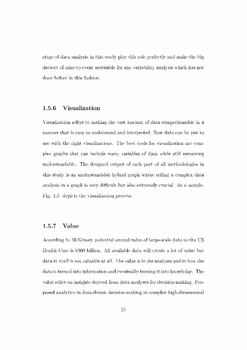
Fig. 2.1 simply illustrated four aforementioned functions:

32

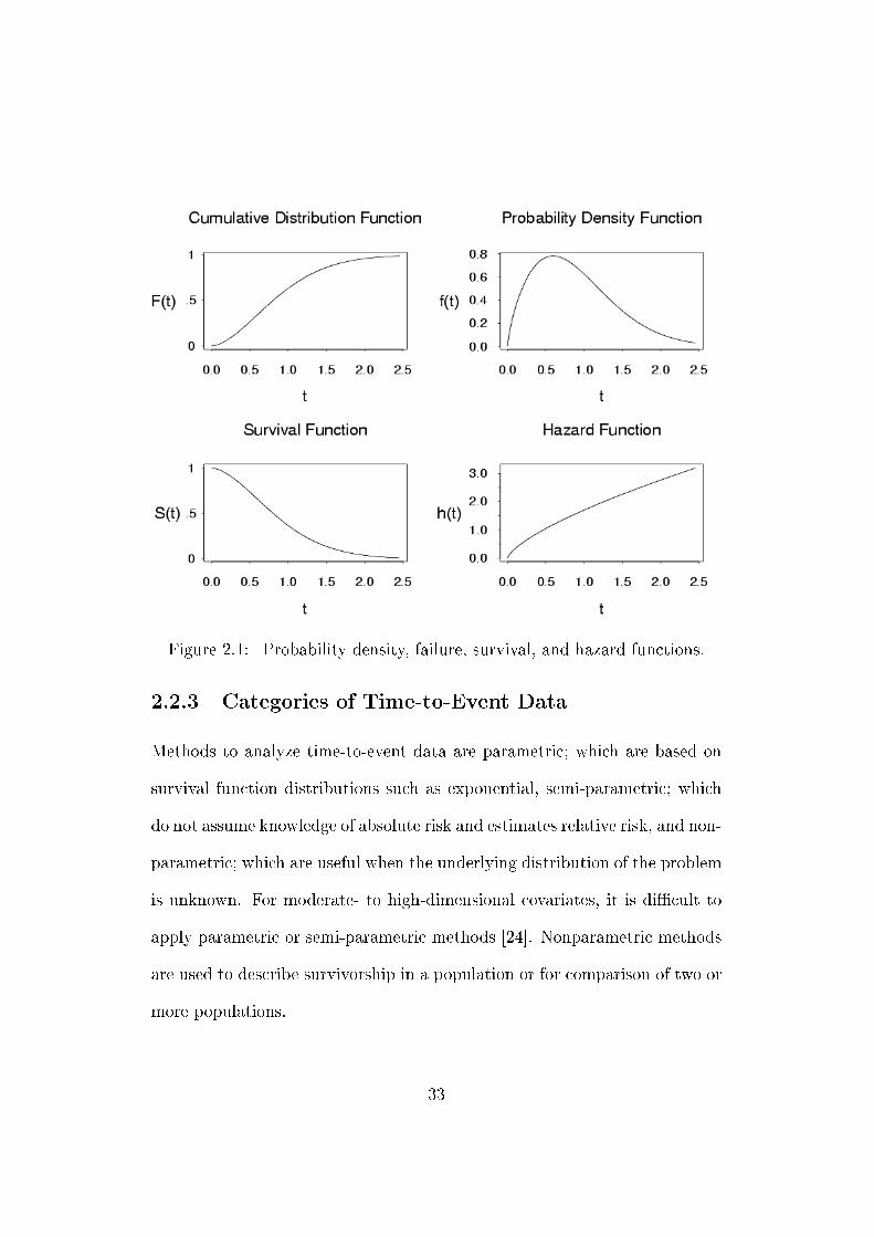
Figure 2.1: Probability density, failure, survival, and hazard functions.

2.2.3 Categories of Time-to-Event Data

Methods to analyze time-to-event data are parametric; which are based on

survival function distributions such as exponential, semi-parametric; which

do not assume knowledge of absolute risk and estimates relative risk, and non-

parametric; which are useful when the underlying distribution of the problem

is unknown. For moderate- to high-dimensional covariates, it is dicult to

apply parametric or semi-parametric methods [24]. Nonparametric methods

are used to describe survivorship in a population or for comparison of two or

more populations.

33

2.2.4 KaplanMeier Estimator

The KaplanMeier (KM) is the most commonly used nonparametric method

for the survival function and has clear advantages since it does not require

an approximation that results the division of follow-up time assumption [23,

33]. Nonparametric estimate of S(t) according to this estimator for distinct

ordered event times t1 to tn is:

S(t) =t∏i=1

(1− dini

) (2.11)

Where at each event time tj there are nj subjects at risk and dj is the number

of subjects which experienced the event. Let ci denote the number of subjects

censored between ti and ti+1. Then the likelihood function takes the form:

L =t∏i=1

[S (ti−1)− S (ti)]di [S (ti)]

ci (2.12)

For the conditional probability of surviving, if we dene πi = S(ti)S(ti−1)

, then

the maximum-likelihood estimation of πi is:

πi = 1− dini

(2.13)

Graphically, the Kaplan-Meier estimate is a step function with discontinu-

ities or jumps at the observed failure times as shown in Fig. 2.2. It has been

shown [44] that the K-M estimator is consistent. Completely nonparametric

nature of this estimator assures little or no loss in eciency using it in prac-

tice.

34

2 4 6 8 10 12 14 16 18 20 220

0.1

0.2

0.3

0.4

0.5

0.6

0.7

0.8

0.9

1

time, t

surv

ival

pro

babi

lity,

s(t

)

Figure 2.2: Kaplan-Meier estimate.

Accelerated failure time model is presented next.

2.3 Accelerated Failure Time Model

In time-to-event data analysis, when distribution of the event time as a re-

sponse variable is unknown, especially in presence of censored observations,

35

estimations and inferences become challenging and the traditional statisti-

cal methods are not practical. Cox proportional hazards model (PHM) [11]

and the accelerated failure time (AFT) [31] are frequently used in these cir-

cumstances. For a comprehensive comparison see [40]. Similar to a multiple

linear regression model, AFT assumes a direct relation between the logarithm

of the time-to-event and the explanatory variables.

As dened in Section 2.2, the event time may not always be observable. This

is known as censored data. In this situation the response variable is dened

as:

Ti = min (Yi, Ci), δi =

1, Yi ≤ Ci

0, Yi > Ci

i = 1 . . . n (2.14)

The censoring time C is independent of the event time Y . Time-independent

explanatory variableXj, j = 1 . . . p corresponding ith observation eects mul-

tiplicatively on the time-to-event Yi or additively on Ti where the relation

between the explanatory variables and the response variable is considered

linear. The AFT model generally is written as:

S(t|x) = S0(t

ψ (x))S0(.) (2.15)

is the baseline survival function and ψ(x) is an acceleration factor dened as

follows:

36

ψ(x) = eβX (2.16)

The coecient vector β is of length-p. The corresponding log-linear form of

the AFT model with respect to time is given by

ln (T ) = Xβ + ε (2.17)

Nonparametric maximum likelihood estimation does not work properly in the

AFT model [62], where in many studies least squares method has been used

to estimate parameters. To account for censoring, weighted least squares

method is commonly used, as ordinary least squares does not work for cen-

sored data in the AFTmodel. According to Stute [55] to obtain estimators us-

ing weighted least squares, a general hypotheses is under the assumption that

vector ε consists of random disturbances with zero mean so that E [ε|X] = 0.

In many studies the error distribution is unspecied [29]. Also for this vector

the assumption of homoscedasticity is supported which assumes a constant

variance for the errors. In addition, regardless of the values of the coecients

and explanatory variables, the log form assures that the predicted values of

T are positive.

Next, a review of decision-making process is presented.

37

2.4 Decision-Making Process

Decision-making is a process of making choices by setting objectives, gath-

ering information, and assessing alternative choices. This process includes

seven steps:

1. Identifying a problem or an opportunity

2. Gathering relevant information

3. Analyzing the problem and information

4. Establishing several possible options and alternative solutions

5. Evaluating alternatives for feasibility, acceptability and desirability.

6. Selecting a preferred alternative for future possible adverse consequences.

7. Implementing and evaluating the solution

Decision-making theories are classied based on two attributes: (a) Deter-

ministic, which deals with a logical preference relation for any given ac-

tion or Probabilistic, which postulate a probability function instead, and

(b) Static, which assume the preference relation or probability function as

time-independent or Dynamic which assume time-dependent events [9]. His-

torically, the Deterministic-Static decision-making is more popular decision-

making process specically under uncertainty. The assumption of decision-

making in this study falls in this category as well.

38

A major part of decision-making involves the analysis of a nite set of al-

ternatives described in terms of evaluative criteria. The mathematical tech-

niques of decision-making are among the most valuable factors of this pro-

cess, which are generally referred to as realization in the quantitative meth-

ods of decision-making [51]. With the increasing complexity and the variety

of decision-making problems due to the huge size of data, the process of

decision-making becomes more valuable. In most decision-making problems,

the multiplicity of criteria for evaluating the alternatives is pervasive [7, 51].

The application of decision-making process in economics, psychology, man-

agement, mathematics, statistics and engineering is obvious and this process

is an important part of all science-based professions. In this study, a decision-

making problem is assumed to be (1) deterministic, which deals with a log-

ical preference relation for any given action and (2) static, which consider

the preference relation or probability function as time-independent. A brief

review of time-to-event data analysis and survival function is following.

The performance of the decision-making process may be aected by a set of

dierent factors includes data size, the number of variables, and the presence

of special cases such as censored or missing data.

A review of commonly used data analysis tools and techniques in this study

is following.

39

2.5 Data Analysis Tools and Techniques

Discretization process, randomization process, and data reduction methods

are reviewed briey.

2.5.1 Discretization Process

Variables in a dataset potentially are a combination format of dierent data

types such as:

Dichotomous (Binary); that occur in one of two possible states,

often labelled zero and one. E.g., improved: yes/no or failed: yes/no.

Nominal; that the values can be assigned a code in the form of a labels

number which is countable but not be ordered or measured. E.g., male

and female (coded in order as 0 and 1)

Ordinal; that can be ranked or rated which could be even counted or

ordered but not measured. E.g., anxiety scale: none, mild, moderate,

and severe, with numerical values of 0, 1, 2, 3.

Categorical; that the value indicates membership in one of several

possible non-overlapping categories. E.g., color: black, brown, red, etc.

If the categories are assigned numerical values used as labels then it

will be synonym for nominal.

40

Discrete; that have only integer values. E.g., the number of a specic

component in warehouse.

Continuous (Interval); that is not restricted to particular values and

may take any value within a nite or innite interval. E.g., days of hos-

pital stay or human reaction or temperature.

There are many advantages of using discrete values over continuous as dis-

crete variables are easy to understand and utilize, more compact and more

accurate. Quantizing continuous variables is called discretization process.

In the splitting discretization methods, continuous ranges are divided into

sub-ranges by the user specied width considering range of values or fre-

quency of the observation values in each interval, respectively called equal-

width and equal-frequency. A typical algorithm for splitting discretization

process which quanties one continuous feature at a time generally consists of

four steps: (1) sort the feature values, (2) evaluate an appropriate cut-point,

(3) split the range of continuous values according to the cut-point, and (4)

stop when a stopping criterion satises.

In this study, discretization of explanatory variables of time-to-event dataset

assumed unsupervised, static, global and direct in order to reach a top-down

splitting approach and transformation of all types of variables in dataset

into a logical (binary) format. Briey, static discretization is dependent of

41

classication task, global discretization uses the entire observation space to

discretize, and direct methods divide the range of k intervals simultaneously.

For a comprehensive study of discretization process, see [34].

2.5.2 Randomization Process

Randomization is the process to select or assign subjects with the same

chance. Many procedures and methods have been proposed for the ran-

dom assignment such as simple, replacement, block, stratied, and covariate

adaptive randomization. To select an appropriate method to produce in-

terpretable and valid results in specic study, knowledge of advantages and

disadvantages of each method is necessary. In this study we briey review

simple and block randomization [56].

Simple randomization keeps complete randomness of the assignment of a

subject to a particular group based on a single sequence of random assign-

ments. This randomization approach is simple and easy to implement. Sim-

ple randomization may be conducted with or without replacement. In simple

replacement randomization, some selection criteria is benecial to use such

as subject stopping criteria which guarantees that one subject could not be

selected more than a specic number.

Block randomization is designed to randomize subjects into equal sample

42

sizes groups. This method is used to ensure a balance in sample size across

groups over time. Blocks are balanced with predetermined group assignment,

which keeps the numbers of subjects in each group similar where the block

size is determined by the researcher as well. Sometimes it is desired to assign

a group (cluster) of subjects together in a cluster randomized trial. The pro-

cedures for block randomizing clusters are identical to those described above.

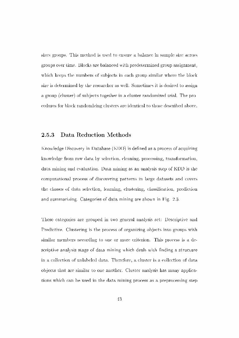
2.5.3 Data Reduction Methods

Knowledge Discovery in Database (KDD) is dened as a process of acquiring

knowledge from raw data by selection, cleaning, processing, transformation,

data mining and evaluation. Data mining as an analysis step of KDD is the

computational process of discovering patterns in large datasets and covers

the classes of data selection, learning, clustering, classication, prediction

and summarizing. Categories of data mining are shown in Fig. 2.3.

These categories are grouped in two general analysis set: Descriptive and

Predictive. Clustering is the process of organizing objects into groups with

similar members according to one or more criterion. This process is a de-

scriptive analysis stage of data mining which deals with nding a structure

in a collection of unlabeled data. Therefore, a cluster is a collection of data

objects that are similar to one another. Cluster analysis has many applica-

tions which can be used in the data mining process as a preprocessing step

43

Figure 2.3: Data mining categories.

for other data mining algorithms [56]. Unsupervised clustering techniques

have been applied to many important problems.

Data reduction techniques are categorized in three main strategies, includ-

ing dimensionality reduction, numerosity reduction, and data compression

[56,57].

Dimensionality reduction as the most ecient strategy in the eld of large-

scale data deals with reducing the number of random variables or attributes in

the special circumstances of the problem. Dimensionality reduction methods

are mainly wavelet transforms and principal components analysis (PCA) [1,

30] which is also known as singular value decomposition (SVD) and Karhunen-

44

Loeve transform (KLV) [18] for transformation and projection of the original

data for elimination of a subset of the original data in terms of variables

covariance.

Numerosity reduction includes techniques substitute the original data by a

smaller alternative set. The methods are parametric which mainly retains

only data estimated parameters instead of original data such as regression

and nonparametric which stores reduced representations of the data such as

histograms, sampling and clustering.

Data compression strategy deals with transformations of data to reach the

compressed representation of the original data. These methods, depends on

the applied algorithm, may cause loose of data during the process of recon-

struction of the data.

2.5.4 Feature Extraction and Feature Selection

All dimensionality reduction strategies and techniques are also classied as

feature extraction and feature selection approaches.

Feature extraction is dened as transforming the original data into a new

lower dimensional space through some functional mapping such as PCA

and SVD [2, 42]. Most unsupervised dimensionality reduction techniques

45

are closely related to PCA, but this technique is not applicable to large

datasets [61].

Feature selection is denoted as electing a subset of the original data (fea-

tures) without a transformation based on some criteria in order to lter out

irrelevant or redundant features, such as lter methods, wrapper methods

and embedded methods [19,52].

Although a broad understanding of all methods is not easy, general knowl-

edge of the area categorizations is recommended in this study. Utilization

of any mathematical model, algorithm and technique requires a complete

knowledge of the purposes of solving the problem. For instance, selecting

a proper class of dimensionality reduction such as feature selection (PCA,

SVD, etc.) or feature extraction (ltering, wrapper and embedded) needs

appropriate characterizing of the problem. Similarly, determining whether

the data in the problem need a supervised or unsupervised method is a major

part of analysis process which leads one to use appropriate techniques.

2.5.5 Principal Component Analysis

Principal Component Analysis (PCA) is one of oldest and most well-known,

appropriate and applicable multivariate analysis techniques which is widely

used to reduce dimensionality of data, enable one to transforms data, even

46

linear or nonlinear, from higher to lower dimension as needed. This reduc-

tion, if performs correctly, eliminates noise, redundant and undesirable data,

retains the most of the useful data, saves resources such as time and mem-

ory used in data processing, as well as generating new signicant features,

variables and attributes [1, 30].

Basically, the principal function of PCA is rotational transformation the axes

of data space along lines of maximum variance, as shown in Fig. 2.4, when

the new axes are called principal component in order, based on their vari-

ance magnitude. The dimensionality reduction could be made by selecting

rst few principal components considering the fact of keeping necessary data.

According to Jollie [30] The central idea of principal component analysis is

to reduce the dimensionality of a dataset in which there are a large number

of interrelated variables, while retaining as much as possible of the variation

present in the dataset. This reduction is achieved by transforming to a new

set of variables, the principal components, which are uncorrelated, and which

are ordered so that the rst few retain most of the variation present in all of

the original variables.

In the literature, principal components analysis (PCA), singular value de-

composition (SVD) and Karhunen-Loeve transform (KLT) are mostly used

equivalently. In the eld of multivariate statistical analysis, these three terms

47

Figure 2.4: Schema of PCA transformation.

are very similar under certain circumstances but not necessarily identical [19].

Some other relevant terms with PCA in dierent elds are Hotelling trans-

formation, independent component analysis (ICA), factor analysis (FA), em-

pirical orthogonal functions (EOF), proper orthogonal decomposition (POD)

eigenvalue decomposition (EVD), empirical eigenfunction decomposition (EED),

empirical component analysis (ECA), spectral decomposition, and empirical

modal analysis.

Some of suggested widespread methods to determine the appropriate number

of components are [63]:

1) Bartlett's Test; which is an analogous statistical test for component anal-

ysis if the remaining eigenvalues are equal. This method should no longer be

employed.

48

2) Kaiser Criteria (K1); is the most commonly used method suggests to retain

the components whose eigenvalues are greater 1.0 and recommends to remove

the components with eigenvalue of less than the average of the eigenvalues.

Kaiser's method tended to severely overestimate the number of components.

3) Scree Test; is based on a graph of the eigenvalues. The scree test is sim-

ple to apply. The eigenvalues are plotted, a straight line is t through the

smaller values and those falling above the line are retained. In this method

some complications may occur such no obvious break point or more than one

break point. The scree test has been is eective when strong components

are present and it this test has been found to be most accurate with-larger

samples and strong components in non-complex data structure.

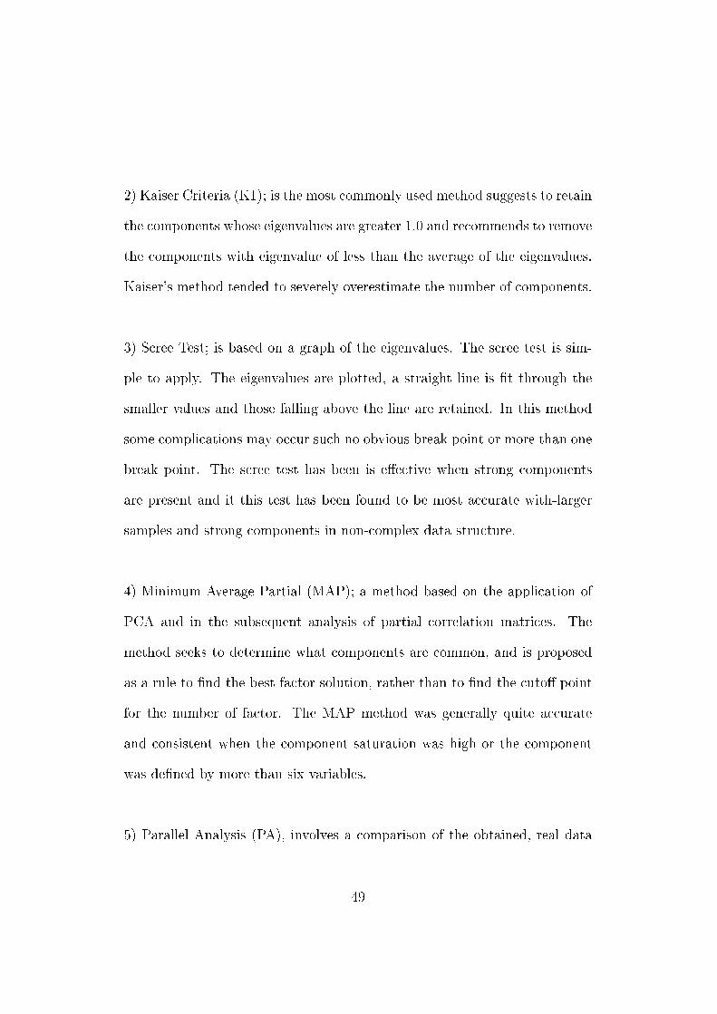
4) Minimum Average Partial (MAP); a method based on the application of

PCA and in the subsequent analysis of partial correlation matrices. The

method seeks to determine what components are common, and is proposed

as a rule to nd the best factor solution, rather than to nd the cuto point

for the number of factor. The MAP method was generally quite accurate

and consistent when the component saturation was high or the component

was dened by more than six variables.

5) Parallel Analysis (PA), involves a comparison of the obtained, real data

49

eigenvalues with the eigenvalues of a correlation matrix of the same rank

and based upon the same number of observations but containing only ran-

dom uncorrelated variables. This method is an adaptation of the K1 rule.

The general application of the PA method is dicult to recommend because

programs needed for its application are not widely available.

50

Chapter 3

Methodology I: Nonparametric

Re-sampling Methods for

KaplanMeier Estimator Test

3.1 Overview

In this chapter, rst proposed analytical model for transformation of the

explanatory variable dataset to reach the logical representation as a sort

of binary variables is presented. Next, in order to select most signicant

variables in terms of ineciency, designed variable selection methods and

heuristic clustering algorithms are introduced [4648].

51

3.2 Analytical Model I

A multipurpose and exible model for a type of time-to-event data with a

large number of variables when the correlation between variables is com-

plicated or unknown is presented. The objective is to simplify the original

covariate dataset into a logical dataset by transformation lemma. Next,

we show the validation of this designed logical model by correlation trans-

formation [47, 48]. The analytic model [47] and its following methods and

algorithms are potentially applicable solutions for many problems in a vast

area of science and technologies.

The random variables Y and C represent the time-to-event and censoring

time, respectively. Time-to-event data is represented by (T,∆, U) where

T = min (Y,C) and the censoring indicator ∆ = 1 if the event occurred, for

instance failure is observed, otherwise 0. The observed covariate U represents

a set of variables. Let denote any observations by (ti, δi, uij), i = 1 . . . n, j =

1 . . . p. It is assumed that the hazard at time t only depends on the survivals

at time t which assures the independent right censoring assumption [31].

The original time-to-event dataset may include any type of explanatory.

Many time-independent variables in U are binary or interchangeable with

a binary variable such as dichotomous variable. Also, interpretation of bi-

52

nary variable is simple, understandable and comprehensible. In addition, the

model is appropriate for fast and low-cost calculation. The general schema of

high-dimensional event history dataset includes n observations with p vari-

ables as shown in Table 3.1.

Table 3.1: Schema for high-dimensional time-to-event dataset.

Obs. # Time to Event Var. 1 Var. 2 . . . Var. p1 t1 u11 u12 . . . u1p

2 t2 u21 u22 . . . u2p

. . . . . . . . . . . . . . . . . .n tn un1 un2 . . . unp

Each array of p variables vectors will take only two possible values, canoni-

cally 0 and 1. As discussed in Chapter 2, discretization method is applied to

values by dividing the range of values for each variable into 2 equally sized

parts. We dene wij as an initial splitting criterion equal to arithmetic mean

of maximum and minimum value of uij for i = 1 . . . n, j = 1 . . . p.

wj =maxuij+ minuij

2i = 1 . . . n, j = 1 . . . p (3.1)

For any array uij in the n-by-p dataset matrix U = [uij], then assign a

substituting array vij as:

53

vij =

0, uij < wij

1, uij ≥ wij

(3.2)

The criteria wij could be dened by expert using experimental or historical

data as well. The proposed model assumes any array with a value of 1 as

desired for expert and 0 otherwise. In other words, vij = 0 represent the lack

of the j th variable in the ith observation. The result of the transformation is

an n-by-p dataset matrix V = [vnp] which will be used in the following meth-

ods and algorithms. Also, we dene time-to-event vector T = [tn] including

all observed event times. The logical model initially could be satised by

proper design of data collection process by based on Boolean logic to gener-

ate binary attributes.

Therefore, the result of the transformation is an n-by-p dataset matrix

V = [vnp] which will be used in the following methods and algorithms. Also,

we dene time-to-event vector T = [tn] including all observed failure times,

and S = [sn] as survival function. The logical model initially could be satis-

ed by proper design of data collection process by based on Boolean logic to

generate binary attributes.

54

3.2.1 Model Validation

Correlation Transformation

To validate the robustness of this model, rst we show that the change of cor-

relation between variables before and after transformation is not signicant

and the logical dataset has followed the same pattern and behavior as the

original; in terms of correlation of covariates. We dene correlation matrix for

each of original and transformed dataset based on Pearson product-moment

correlation coecient; M = [mij] and N = [nij] where i = 1 . . . n, j = 1 . . . p,

where nij and mij denote covariance of variables i and j for original and

transformed dataset respectively as follows:

nij =1

n− 1

n∑k=1

(uik − ui)(ujk − uj) i = 1 . . . p, j = 1 . . . p (3.3)

mij =1

n− 1

n∑k=1

(vik − vi)(vjk − vj) i = 1 . . . p, j = 1 . . . p (3.4)

where (uik, vik) and (ui, vi) represent value of variable i in observation k and

mean of variable i in each dataset respectively, and similarly the second

parenthesis in equations 3.3 and 3.4 are dened for variable j.

The experimental tted line for the scatter plot of mij and nij for anydataset

is y = a+ bx where b is positive small and a is not signicant. For instance,

Fig. 3.1 shows the primary biliary cirrhosis (PBC) dataset (Section 3.2) for

an experimental result of an uncensored data with the tted line of y =

55

−0.4 −0.2 0 0.2 0.4 0.6

−0.5

−0.4

−0.3

−0.2

−0.1

0

0.1

0.2

0.3

0.4

0.5

original dataset

tran

sfor

med

dat

aset

Figure 3.1: Comparison of covariate correlations in the original and thetransformed dataset.

0.0116 + 0.6356x.

The proposed logical model validation and verication of the robustness were

presented comprehensively in [46,48].

Cox Proportional Hazards Model (PHM) Baseline

The next validation is to compare the estimates of the survival and hazard

functions of the original and the transformed dataset to verify the proposed

56

model. Theoretically, a statistical test such as Wilcoxon rank sum test and

log-rank test determine whether we can assume two sample data are equal or

in other words, are collected from identical population. Based on Cox PHM

baseline, if the survival or hazard functions of the original and the trans-

formed dataset are similar, it proves that both datasets are not in-equivalent

in term of hazard rate and the transformation does not change the eect of

complete set of variables on survival function.

Although proportional hazards regression, as well as other multiple regres-

sion models will face several calculation errors dealing with high-dimensional

data especially in with a huge number of covariates, computational methods

show that the variation in the approximation of PHM baselines for equiva-

lent time-to-event datasets is negligible. Comparing empirical product limit

estimate for the survival function of the original with the PHM baseline

survival function of the original dataset and transformed logical dataset in

many tested sample datasets in this study shows that the transformation

of the dataset does not change the nature of the covariates in terms of the

survival function and the hazard function.

Fig. 3.2 depicts the empirical survival function, Cox PHM baseline survival

function for original dataset, and Cox PHM baseline survival function for the

transformed logical uncensored PBC dataset (Section 3.3). The Wilcoxon

test score of comparing nonparametric baseline survival function of the orig-

57

inal dataset and transformed logical dataset is 0.9704 and according to the

test concept, it shows that these two functions are not unequal. This result

proves that we should expect no signicant change in the covariate correla-

tions due to the proposed transformation. We applied similar validation to

many datasets in this research to verify this analytic model.

0 500 1000 1500 2000 2500 3000 3500 4000 4500 50000

0.1

0.2

0.3

0.4

0.5

0.6

0.7

0.8

0.9

1

time,t

surv

ival

pro

babi

lity,

s(t)

Figure 3.2: Empirical survival function (solid blue), Cox PHM baseline sur-vival function for the original dataset (black dashed), and Cox PHM baselinesurvival function for transformed logical dataset (red dotted).

In order to select the most signicant variables in terms of ineciency, de-

signed methods and heuristic algorithms are presented next.

58

3.3 Methods and Algorithms for Variable Se-

lection

We design a class of methods applying on proposed logical model to select

inecient variables in a high-dimensional event history datasets. The ma-

jor assumption to design appropriate methods for this purpose is that the

variable which is completely inecient solely can provide a signicant per-

formance improvement when engaged with others, and two variables that

are inecient by themselves can be ecient together [19]. Based on this

assumption, we design three methods and heuristic algorithms to select in-

ecient variables in event history datasets with high-dimensional covariates.

We use Kaplan-Meier estimator in this study to estimate survival probabili-

ties as a function of time. A nonparametric test could be used to test a null

hypothesis that whether two samples are drawn from the same distribution,

as compared to a given alternative hypothesis. Among many nonparametric

tests for comparing survival functions for aforementioned propose, we use

log-rank test in our methods as a best t for comparison of two nonparamet-

ric distributions. This test is the most commonly used for a typical study

under dierent models for the relationship between the groups [24,32].

The n-by-p matrix V is the prepared transformed logical dataset according

59

to Section 3.1, where n is the number of observations, p is the number of

variables, and k is the estimated subset size to select for calculation parts in

the algorithms.

Recalling V which is constructed by k observation vectors corresponding to

each of the variables, D = [dkp] as a k -by-p matrix is a selected subset of V

and k is dened as the number of observations in any subset of V , where

k ≤ n. For any variable i, we dene vectorO i as a time-to-event vector which

includes failure times of any observation j the value of vij is one. Similarly,

we dene vector Z i including failure times of any observation j where the

value of vij is zero. The vectors R and S are dened as follow:

ri =

ti,∑di. ≥ 0

0, Otherwisei = 1 . . . n (3.5)

si =

ti,∏di. = 1

0, Otherwisei = 1 . . . n (3.6)

Vector R is constructed by all non-zero arrays r and similarly vector S is

constructed by all non-zero arrays s.

A class of methods and algorithms to select inecient variables are following:

60

3.3.1 Singular Variable Eect

The objective of Singular Variable Eect (SVE) method is to determine the

eciency of a variable by analyzing the eect of the presence of any variable

singularly in comparison with its absence in a transformed logical dataset.

For p variable, we aim to set vector ∆ = [δi ] where i = 1 . . . p to rank the

eciency of the variables. The preliminary step for the highest eciency in

this method is to initially clustering the variables based on the correlation

coecient matrix of original dataset, M , and choose a representative vari-

able from each highly correlated cluster and eliminate the other variables

from the dataset. For instance, for any given dataset, if three variables are

highly correlated, only one of them is selected randomly and the other two

are eliminated from the dataset. The result of this process assures that the

remaining variables for applying methods and heuristic algorithms are not

highly correlated.

As an outcome of the SVE procedure, if one hopes to reduce the number

of variables in the dataset for further analysis, could eliminate less ecient

identied variables or if aims to concentrate on a reduced number of vari-

ables, could choose a category of more ecient identied variables as well.

Heuristic algorithm for SVE method is:

for i = 1 to p do

61

Calculate O i and Z i for variable i observation vector in dataset V

Compare T and O i with Wilcoxon rank sum test

Save the test score for variable i as αi

Compare T and O i with Wilcoxon rank sum test

Save the test score for variable i as βi

Calculate δi = αi - βi

end for

Return ∆ = [δp] as the variable eciency vector

3.3.2 Nonparametric Test Score

The log-rank test score variable selection method is applied for selecting a

subset of the best and the worst variables in terms of eciency. The Non-

parametric Test Score (NTS) method is a variable clustering technique which

selects set of size k variables from the transformed logical dataset V and cal-

culates the score of each variable in two levels. The rst level is to determine

the priority of the variable eciency via the score reached by the frequency

of the presence of each variable from the rejected subsets in comparison with

the original time-to-even vector T . We code this level of calculation with

letter F. The second level rates the variables by the cumulative score of each

variable from comparisons of selected subsets of all nonparametric test re-

sults with the original time-to-even vector T . This level acts as a searching

62

procedure to detect the less ecient variables. The code which this level is

denoted by is the letter C. Randomization (RN) algorithm randomly chooses

a dened l subset of k from the V , transformed logical dataset of p vari-

able. We dene a randomization dataset matrix Ψ = [ψlk] where each row

is formed by k variable identication numbers in any selected subsets for

overall l subsets. Heuristic algorithm of NTS method level F is:

for i = 1 to q do

Compose the dataset D i for variable set i in Ψ including variables

ψij where j = 1 to k

Calculate Ri over the dataset D i

Compare T and Ri with log-rank test

Save the test score for variables in subset i as ψi(k+1)

end for

Eliminate rows of Ψ where the array k+1 of the row has a value of more

than 0.05, and call this new set Ψ*

Count the contribution (presence) of each variable h based on its

identication number in the

Ψ* rst k columns and save as γh

Return Γ = [γp] as the variable eciency vector

63

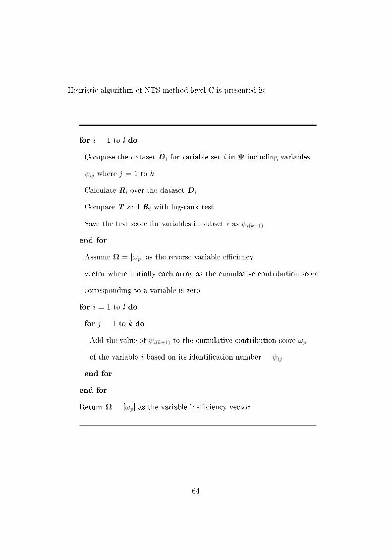
Heuristic algorithm of NTS method level C is presented is:

for i = 1 to l do

Compose the dataset D i for variable set i in Ψ including variables

ψij where j = 1 to k

Calculate Ri over the dataset D i

Compare T and Ri with log-rank test

Save the test score for variables in subset i as ψi(k+1)

end for

Assume Ω = [ωp] as the reverse variable eciency

vector where initially each array as the cumulative contribution score

corresponding to a variable is zero

for i = 1 to l do

for j = 1 to k do

Add the value of ψi(k+1) to the cumulative contribution score ωp

of the variable i based on its identication number = ψij

end for

end for

Return Ω = [ωp] as the variable ineciency vector

64

3.3.3 Splitting Semi-Greedy Clustering

Splitting Semi-Greedy (SSG) method to select an inecient variable subset

is proposed. A clustering procedure through randomly splitting approach

to select the best local subset according to a dened criterion incorporated.

In this method we use block randomization which is designed to randomize

subjects into equal sample sizes groups. A nonparametric test is used to

test a null hypothesis that whether two samples are drawn from the same

distribution, as compared by a given alternative hypothesis. Wilcoxon rank

sum test is used in this method.

The concept of this method is inspired by the semi-greedy heuristic [14, 20]

and tabu search [17]. Criterion of this search is similar to The Nonpara-

metric Test Score (NTS) method [48] which is to collect the most inecient

variable subset via Wilcoxon rank sum test score. At each of l trials, all

p variables from the transformed logical dataset V are randomly clustered

into subsets of size k variables, where one cluster possibly contains less than

k variables and the number of clusters is equal to dp/ke. To calculated score

summation for each variable over all trials, a randomization dataset matrix

Ξ = [ξlk] where each row is formed by k variable identication numbers

in any selected subsets for all l trials. Comprehensive experimental results

for validation of the proposed methods by comparison with similar methods

are presented in Sections 3.4 and 3.5. Heuristic algorithm for SSG method is:

65

for i = 1 to l do

Split the data into equally sized subsets

Compose the dataset D for each subset

Calculate R over the D for each subset

Compare T and R with Wilcoxon rank sum test and save the test score

for each subset one by one

Select a subset with the highest test score

Save the test score for variables in the selected subset as ξi(k+1)

end for

Assume Θ = [θp] as the reverse variable eciency vector

where initially each array as the cumulative contribution score

corresponding to a variable is zero

for i = 1 to l do

for j = 1 to k do

Add the value of ξi(k+1) to the cumulative contribution score θp

of the variable i based on its identication number = ξij

end for

end for

Return Θ = [θp] as the variable ineciency vector

66

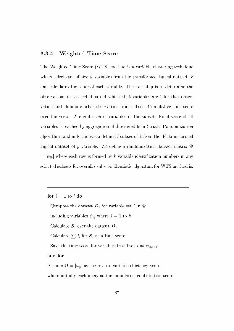
3.3.4 Weighted Time Score

The Weighted Time Score (WTS) method is a variable clustering technique

which selects set of size k variables from the transformed logical dataset V

and calculates the score of each variable. The rst step is to determine the

observations in a selected subset which all k variables are 1 for that obser-

vation and eliminate other observation from subset. Cumulative time score

over the vector T credit each of variables in the subset. Final score of all

variables is reached by aggregation of those credits in l trials. Randomization

algorithm randomly chooses a dened l subset of k from the V , transformed

logical dataset of p variable. We dene a randomization dataset matrix Ψ

= [ψlk] where each row is formed by k variable identication numbers in any

selected subsets for overall l subsets. Heuristic algorithm for WTS method is:

for i = 1 to l do

Compose the dataset D i for variable set i in Ψ

including variables ψij where j = 1 to k

Calculate S i over the dataset D i

Calculate∑

ti for S i as a time score

Save the time score for variables in subset i as ψi(k+1)

end for

Assume Ω = [ωp] as the reverse variable eciency vector

where initially each array as the cumulative contribution score

67

corresponding to a variable is zero

for i = 1 to l do

for j = 1 to k do

Add the value of ψi(k+1) to the cumulative contribution score ωp

of thevariable i based on its identication number = ψij

end for

end for

Return Ω = [ωp] as the variable ineciency vector

Comprehensive experimental results for validation of the proposed methods

by comparison with similar methods for right-censored dataset (Section 3.4)

and uncensored dataset (Section 3.5) are presented next.

3.4 Experimental Results and Analysis for Right-

Censored Data

To evaluate the performance of the proposed methods for right-censored data,

NTS and SSG methods and algorithms under dierent types of datasets in-

cluding collected and simulated data is investigated. In order to obtain an

estimation of desired number of variables in any selected subset of these

methods for calculations in hybrid algorithms, we use principal component

68

analysis (PCA) scree plot criterion [63]. The criterion for this evaluation is

based on eigenvalue of components in a dataset. The cut-o in the scree plot

is interpreted as a set of signicant eigenvalues among all components which

leads to determine k, number of ecient variables in a given dataset. We

apply this technique on the original dataset to determine k.

First, the well-known primary biliary cirrhosis (PBC) dataset (Fleming and

Harrington 1991) is considered as the sample collected dataset. These data

are from a double-blinded randomized trial including 312 observations. This

right-censored dataset contains 17 variables in addition to censoring infor-

mation, identication number and event times for each observation. Experi-

mental results for the 276 observations with complete records are presented

(36 out of 312 observations are incomplete). For the original PBC dataset,

approximate value of k is 3. This value is the subset size in the algorithms

applied on V transformed logical dataset n-by-p matrix, shown in Fig. 3.3.

Another set up before applying methods and algorithms is to preliminary de-

termine which variables are more behaving similarly, using modied k-means

clustering algorithm. Basically, k-mean algorithm partitions the points in the

n-by-p dataset matrix into k clusters. The default of calculation is Squared

Euclidean distance. Our modied k-mean algorithm changes the dimension

of transformed logical dataset and returns clusters of the variables in terms

of the observation. The result gives us an acceptable view of expected clus-

69

0 2 4 6 8 10 12 14 16 180

0.5

1

1.5

2

2.5

3

3.5

4

4.5

5x 10

4

component number

eige

nval

ue

Figure 3.3: Scree plot of the original PBC dataset including 17 variablesand 276 observations.

tering in the next parts. Number of clusters is calculated by the quotient`s

nearest integer value of the number of the dataset variables p divided by the

number of the subset variables k. The result of this preliminary evaluation

for the transformed logical uncensored PBC dataset is shown in Table 3.2.

To verify the performance of the proposed methods, the result of methods

and algorithms for the transformed logical PBC dataset is compared with the

Random Survival Forest (RSF) method results [27,28], Additive Risk Model

70

Table 3.2: Modied k-means clustering algorithm result for the transformedlogical uncensored PBC dataset. Number of clusters is equal to ‖ p

k‖.

Cluster # Variable #1 4, 6, 72 3, 5, 10, 173 14 25 8, 9, 11, 12, 13, 14, 15, 16

(ADD) [36], and Weighted Least Square (LS) [24] results for variable selec-

tion in PBC dataset are given in Table 3.3. A comprehensive comparison

of RSF, ADD and LS performance with other relevant methods in high-

dimensional time-to-event data analysis such as Cox's Proportional Hazard

Model, LASSO and PCR has been presented in [24,28,36].

The survival function results of NTS-RN algorithm for 100 trials on the trans-

formed logical uncensored PBC dataset is shown in Fig. 3.4.

Each number in Tables 3.3 and 3.4 represents a specic variable in experi-

ment dataset. For example, in Table 3.3, variable #15 is among the selected

less ecient variables by methods NTS (F), SSG, RSF and LS.

From the results shown on Tables 3.3, the NTS (F) method has closest per-

formance to the SSG. This is an advantage of these methods that more than

80% of inecient variables which has been detected by other methods (RSF,

71

Figure 3.4: Empirical transformed logical uncensored PBC dataset survivalfunction (solid red) with 99% condence bounds (red dotted). Subset of kvariable with failed to reject Wilcoxon rank sum test result (gray), and subsetof k variable with rejected Wilcoxon rank sum test result (black).

LS and ADD) are collected by proposed algorithms at signicantly short pe-

riod of calculation. The robustness of this class of methods has examined for

several sample collected time-to-event data with high-dimensional covariates

in this study.

Continuing the validation of the proposed methods, we set n = 400 observa-

tions and p = 25 variables and simulated event times from a pseudorandom

algorithm. In addition to constant and periodic binary numbers, normal and

exponential distributed pseudorandom numbers are generated as indepen-

dent values of explanatory variables. The censored observations were also

72

Table 3.3: Selected less ecient variables in all proposed methods and com-parison to RSF, ADD, and LS method results.

Method Selected Less Ecient VariablesNTS (F) 1, 3, 5, 6, 10, 15, 17NTS (C) 2, 5, 10, 11, 13, 17SSG 1, 3, 5, 10, 15, 17RSF 1, 3, 5, 12, 13, 14, 15, 17ADD 1, 2, 5, 12, 14LS 1, 2, 3, 14, 15, 17

generated independent of the events. Additionally, some variables are set as

a linear function of event time intentionally. We present the results of meth-

ods and algorithms applying the simulated data in Table 3.4. These results

are compared with the simulation dened pattern and the comparison veries

the performance of all proposed methods and algorithms. In the simulation,

dened pattern includes ve inecient variables, No. 5, 10, 15, 20, and 25.

Table 3.4: Selected less ecient variables in all proposed methods and com-parison to simulation dened pattern.

Method Selected Less Ecient VariablesNTS (F) 5, 10, 25NTS (C) 5, 10, 25SSG 5, 10, 25

Denition 5, 10, 15, 20, 25

Ineciency analysis results for the simulation experiment shows that vari-

73

ables with identication number 5, 10 and 25 are detected as less ecient

variables among all 25 simulated variables by NTS (F), NTS (C) and SSG

methods. In this example, one could eliminate these less ecient identied

variables if the objective is to reduce the number of variables in the dataset

for further analysis.

In addition, a set of simulation numerical experiments are presented to eval-

uate performance of the proposed methods as shown in Table 3.5. For that,

six dierent simulation models are dened. Setting of these models are as

explained above for n = 400 observations and p = 25 variables following

same data generating algorithm. Number of signicant inecient variables

in each simulation model in order are m = 4, 5, 6 as presented in De-

nition in Table 3.5. The simulations are repeated 100 times independently.

For each method, m represents integer average number of determined and

selected inecient variables and p denotes performance of the method, for

100 trails, where

p = mmethod/mdefinition (3.7)

and p is the average of performance of each method. The adjusted censoring

rates for all simulation numerical experiments are 50± 5%.

Graphical tool for interpretation of the results for proposed methods, hybrid

scattering for variable ineciency for three criteria as (a) NTS (F) score, (b)

NTS (C) score and (c) SSG score for PBC data experiment results is displayed

74

Table 3.5: Performance of the proposed methods based on six simulationnumerical experiment. m is integer average number of selected inecientvariable and p is performance of method based on 100 replications.

#1 #2 #3 #4 #5 #6 AveMethod m p m p m p m p m p m p pNTS (F) 3 0.75 3 0.75 3 0.60 4 0.80 4 0.67 5 0.83 0.73NTS (C) 3 0.75 3 0.75 4 0.80 4 0.80 5 0.8 5 0.83 0.79SSG 2 0.50 3 0.75 3 0.60 4 0.80 4 0.67 4 0.67 0.66

Denition 4 4 5 5 6 6

in Fig. 3.5. Each variable is exposed by a circle icon where two axes repre-

sent the standardized criterion (a) and (b) and the diameter of each circle

demonstrate the standardized criterion (c). These ineciency score criteria

are standardized in the range of [0, 25] and for clear graphics presentation,

plot range is [−5, 25]. Therefore, it is interpreted from the hybrid scatter plot

that each variable with larger diameter and more distance from the center has

less eciency and is an ideal candidate to remove from dataset if it is desired.

3.5 Experimental Results and Analysis for Un-

censored Data

To evaluate the performance of the designed methods for uncensored data,

rst PBC dataset is considered as the sample collected dataset. The pur-

pose of this section is to examine and validate the proposed methods in

75

−5 0 5 10 15 20 25−5

0

5

10

15

20

25

1

2

3

4

56

7

89

10

1112

13

14

15

16

17

criterion a

crite

rion

b

Figure 3.5: Hybrid scatter plot - Upper right variables have less eciency.

this chapter with uncensored time-to-event data. These dataset includes 111

uncensored complete observations and 17 explanatory variables. To verify

the performance of the proposed methods for uncensored data, the result of

these methods and algorithms for the transformed logical uncensored PBC

dataset including 111 uncensored complete observations and 17 explanatory

variables is compared with the results of Nonparametric Test Score (NTS)

method [48], Random Survival Forest (RSF) method [27, 28], Additive Risk

Model (ADD) [36], and Weighted Least Square (LS) method [24] for similar

76

dataset variable selection, given in Table 3.6.

Each number in Tables 3.6 and 3.7 represents a specic variable in experi-

ment dataset. For example, in Table 3.6, variable #1 is determined from the

results as an inecient variable by all methods.

Table 3.6: Selected inecient variables in all proposed methods and compar-ison to NTS, RSF, ADD, and LS method results.

Method Selected Inecient VariablesSVE 1, 3, 5, 10, 13, 17SSG 1, 3, 5, 10, 15, 17WTS 1, 3, 5, 10, 15, 17NTS 1, 3, 5, 6, 10, 15, 17RSF 1, 3, 5, 12, 13, 14, 15, 17ADD 1, 2, 5, 12, 14LS 1, 2, 3, 14, 15, 17

From the results shown on Tables 1, the SSG and WTS methods have a same

performance. More than 80% of inecient variables which has been detected

by other methods (NTS, RSF, LS and ADD) are collected by proposed al-

gorithms at signicantly shorter calculation period, where the robustness of

this class of methods has examined for several sample datasets.

To show variable ineciency through three designed methods SVE, SSG,

and WTS, graphical representation for the experiment results for uncen-

sored PBC dataset is depicted in Fig. 3.6. Each variable with larger radius

77

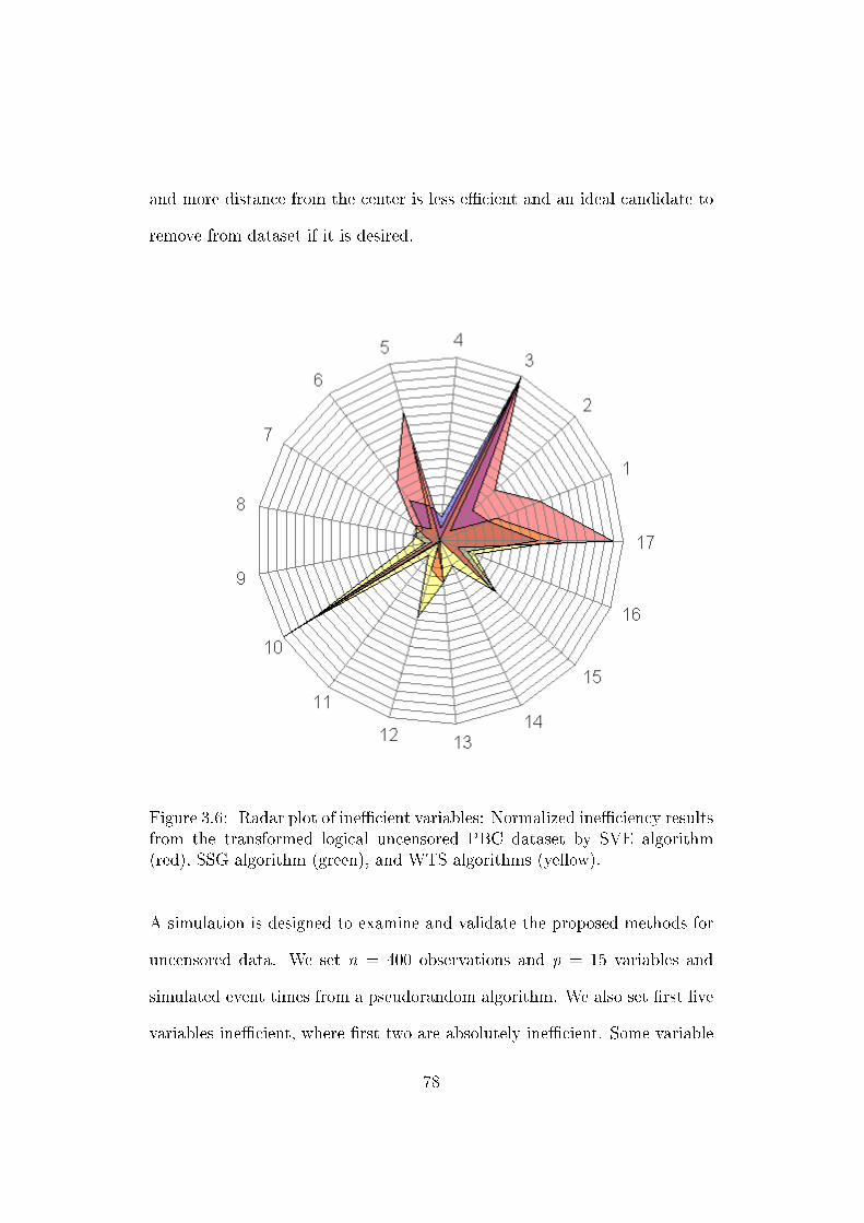
and more distance from the center is less ecient and an ideal candidate to

remove from dataset if it is desired.

Figure 3.6: Radar plot of inecient variables: Normalized ineciency resultsfrom the transformed logical uncensored PBC dataset by SVE algorithm(red), SSG algorithm (green), and WTS algorithms (yellow).

A simulation is designed to examine and validate the proposed methods for

uncensored data. We set n = 400 observations and p = 15 variables and

simulated event times from a pseudorandom algorithm. We also set rst ve

variables inecient, where rst two are absolutely inecient. Some variable

78

vectors are set as a linear function of event time data in addition to constant

and periodic binary numbers as well as normal and exponential distributed

pseudorandom numbers as independent values of explanatory variables. The

results of methods and algorithms applying the simulated data are presented

in Table 3.7. These results are compared with the results from NTS method.

From the simulation dened pattern as shown in Table 3.7, the comparison

veries the performance of all proposed methods.

Table 3.7: Selected inecient variables in all proposed methods and compar-ison to NTS results and simulation dened pattern.

Method Selected Inecient Variables (No.)SVE 1, 2, 3, 10SSG 1, 2, 3WTS 1, 2, 3, 5, 12NTS 1, 2, 5

Denition 1, 2, 3, 4, 5

Ineciency analysis results for the simulation experiment shows that vari-

ables with identication number 1, 2 and 3 are detected as inecient variables

by all proposed methods. To reduce the number of variables in the dataset

for further analysis, these explanatory variables are the best candidates to

be eliminated from the dataset.

79

Chapter 4

Methodology II: Heuristic

Randomized Decision-Making

Methods through Weighted

Accelerated Failure Time Model

4.1 Overview

This chapter presents an analytical model for normalization the explana-

tory variable dataset to reach an appropriate representative dataset.

Next, designed heuristic randomized decision-making methods and algorithms

80

to select most signicant variables in terms of eciency through accelerated

failure time model are introduced. Then numerical simulation experiment

is developed to investigate the performance and validation of the proposed

methods [12,49].

4.2 Analytical Model II

A simple analytic model to analyze complicated right-censored time-to-event

data with high-dimensional explanatory variables in order to facilitate vari-

able selection procedure in decision-making procedure is developed. Trans-

forming data values into appropriate computational form is a commonly used

approach. There are many advantages of using discrete values over continu-

ous; as discrete variables are easy to understand and utilize, more compact,

and more accurate. In this study, for a time-to-event dataset including dis-

crete values, a normalization analytical model is dened.

As explained in Chapter 2, the random variables Y and C represent the

time-to-event and censoring time, respectively. Time-to-event data is rep-

resented by (T, ∆, U) where Ti = min (Yi, Ci) and the censoring indi-

cator di = 1 if the event occurs, otherwise di = 0. The observed co-

variate U represents a set of variables. Let denote any observations by

(ti, di, uij) , i = 1 . . . n, j = 1 . . . p. It is assumed that the hazard at time t

only depends on the survivals at time t which assures the independent right

81

censoring assumption [31].

Data normalization is a method used to scale data and standardize the range

of independent variables or features of data to allow the comparison of cor-

responding normalized data, also known as feature scaling. As a simple and

well-known rescaling method, unity-based normalization scales in [0, 1] range.

One problem in this process is the appearance of outliers that takes extreme

values and a solution to remove the outliers before normalization could be

using a threshold as below algorithm:

1. Arrange data in order

2. Calculate rst quartile Q1, third quartile Q3, and the interquartile

range IQR = Q3−Q1

3. Compute the range of Q3 + 1.5(IQR) and Q1− 1.5(IQR)

4. Remove any value outside this range as an outlier

The original dataset may include any type of explanatory data as binary,

continuous, categorical, or ordinal data. For any n-by-p dataset matrix

U = [uij], there are n independent observations and p variables. To normal-

ize the dataset, we dene minimum and maximum value of each explanatory

variable value in vector Uj for j = 1 . . . p as:

82

uminj = min uij , umaxj = max uij i = 1 . . . n (4.1)

For any array uij, we allocate a normalized substituting array vij as:

vij =uij − uminj

umaxj − uminji = 1 . . . n, j = 1 . . . p (4.2)

The result of the transformation is an n-by-p dataset matrix V = [vnp] which

will be used in the designed heuristic methods and algorithms. Also, we dene

time-to-event vector T = [tn] including all observed event times. Application

of a robustness validation method proposed by [12,4648], indicates that the

change of correlation between variables before and after transformation is

not signicant.

As a brute-force search algorithm outcome, the all subset models method

is the simplest and computationally consuming which generates all possible

subsets including combinations of p explanatory variables, totally 2p−1 sub-

set. This exhaustive method is not suitable for large numbers of variables.

Another approach is to develop models including combinations of the k vari-

ables, called selective, where 1 ≤ k < p. Consequently the total number of

models is given by:

83

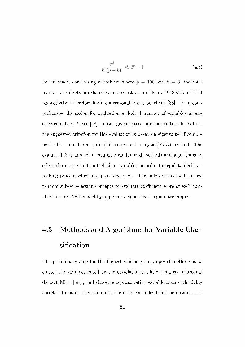
p!

k! (p− k)! 2p − 1 (4.3)

For instance, considering a problem where p = 100 and k = 3, the total

number of subsets in exhaustive and selective models are 1048575 and 1114

respectively. Therefore nding a reasonable k is benecial [38]. For a com-

prehensive discussion for evaluation a desired number of variables in any

selected subset, k, see [48]. In any given dataset and before transformation,

the suggested criterion for this evaluation is based on eigenvalue of compo-

nents determined from principal component analysis (PCA) method. The

evaluated k is applied in heuristic randomized methods and algorithms to

select the most signicant ecient variables in order to regulate decision-

making process which are presented next. The following methods utilize

random subset selection concepts to evaluate coecient score of each vari-

able through AFT model by applying weighed least square technique.

4.3 Methods and Algorithms for Variable Clas-

sication

The preliminary step for the highest eciency in proposed methods is to

cluster the variables based on the correlation coecient matrix of original

dataset M = [mij], and choose a representative variable from each highly

correlated cluster, then eliminate the other variables from the dataset. Let

84

mij denote covariance of variables i and j. Pearson product-moment corre-

lation coecient matrix is dened as

mij =1

n− 1

n∑k=1

(vik − vi)(vjk − vj) i = 1 . . . p, j = 1 . . . p (4.4)

vik and vi in order represent value of variable i in observation k and mean

of variable i, and similarly second parenthesis is dened for variable j. For

instance, for any given dataset if three variables are highly correlated in M,

only one of them is selected randomly and the other two are eliminated from

the dataset. The outcome of this process assures that the remaining variables

for applying methods are not highly correlated.

A method is developed for the proposed normalization model to select e-

cient variables in right-censored time-to-event datasets with high-dimensional

explanatory variables. The basic assumption to design appropriate methods

for this purpose is that the variable which is completely inecient solely

can provide a signicant performance improvement when engaged with oth-

ers, and two variables that are inecient by themselves can be ecient to-

gether [44]. In these methods we use block randomization which is designed

to randomize subjects into equal sample sizes groups. Generally randomiza-

tion is the process to select or assign subjects with the same chance. Many

randomization procedures and methods have been proposed for the random

assignment; such as simple, replacement, block, and stratied [34].

85

To obtain variable coecients estimation, let win be the KM weights. For

i = 1 . . . n these weights can be calculated using the expression

win = S (lnTi )− S(lnTi−1 ) (4.5)

Considering the denition of KM estimator S as equation (2.11), win is ob-

tained [32] by

w1n =d1

n, w

in=

din− i+ 1

i−1∏j=1

(n− j

n− j + 1)di

i = 2 . . . n (4.6)

Recall AFT model 2.17, the estimator of β is

β = argminβ

n∑i=1

win[(ln Ti)− βXi ]2 (4.7)

The matrix calculation leads to an estimator solution as

β = (X′WX)

−1X′Wln T (4.8)

where X′is transpose of X. The equation 4.8 is used to estimate variable

coecients in heuristic decision making methods where X ≡ V.

Determining k as a number of observations in any subset of transformed

normalized data8set V, as described in Section 4.2. Where k ≤ n, then k -

by-p sub-dataset matrix D = [dkp] is dened as a selected subset of V. Also

vector B = [bk] will be utilized in following methods as a coecient estimator

vector corresponding to the explanatory variables for sub-dataset D.

86

In continue, this chapter provides heuristic randomized decision-making al-

gorithms for implementing variable selection through determining variable

eciency recognition procedure based on dened coecient score in right-

censored high-dimensional time-to-event data. The proposed methods utilize

random subset selection concept to evaluate coecient score of each variable

through accelerated failure time model by applying weighed least square tech-

nique.

4.3.1 Ranking Classication

The concept of Ranking Classication (RC) method is inspired by the semi-

greedy heuristic [14,20]. The objective of this method is to introduce ecient

variables in terms of correlation with survival time for an event time through

randomly splitting approach by selecting the best local subset using a coef-

cient score. This method is a ranking classication using semi-greedy ran-

domized procedure to split all explanatory variables into subset of predened

size k citesadeghzadeh2015nonparametric, sadeghzadeh2014multidisciplinary

using equal-width binning technique. The number of bins is equal to

c = dp/ke (4.9)

Note that if p is not divisible by k, then one bin contains less than k variables.

At each of l trials where l is a dened large reasonable number, a local

coecient score is calculated for any variable cluster at any bin. For i′th

87

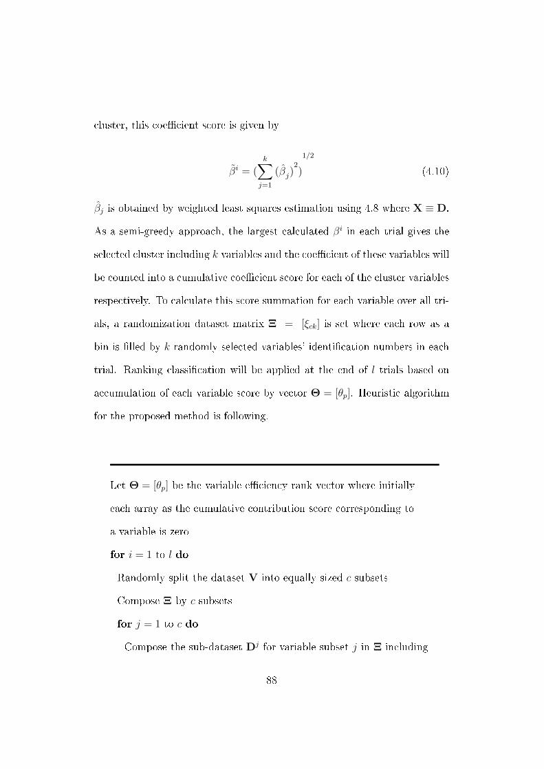
cluster, this coecient score is given by

βi = (k∑j=1

(βj)2)

1/2

(4.10)

βj is obtained by weighted least squares estimation using 4.8 where X ≡ D.

As a semi-greedy approach, the largest calculated βi in each trial gives the

selected cluster including k variables and the coecient of these variables will

be counted into a cumulative coecient score for each of the cluster variables

respectively. To calculate this score summation for each variable over all tri-

als, a randomization dataset matrix Ξ = [ξck] is set where each row as a

bin is lled by k randomly selected variables' identication numbers in each

trial. Ranking classication will be applied at the end of l trials based on

accumulation of each variable score by vector Θ = [θp]. Heuristic algorithm

for the proposed method is following.

Let Θ = [θp] be the variable eciency rank vector where initially

each array as the cumulative contribution score corresponding to

a variable is zero

for i = 1 to l do

Randomly split the dataset V into equally sized c subsets

Compose Ξ by c subsets

for j = 1 to c do

Compose the sub-dataset Dj for variable subset j in Ξ including

88

variables ξjq for q = 1 to k

Calculate Wj over the sub-dataset Dj

Calculate coecient vector Bj over the sub-dataset Dj using

4.8

Calculate coecient score βj corresponding Bj over the

sub-dataset Dj using 4.10

end for

Select a subset with the highest βj, call this new subset D∗

for j = 1 to k do

Add the value of bij corresponding the variable ξij to the cumulative

coecient score θp of the variable q based on its identication

number = ξij

end for

end for

Normalize Θ = [θp]

Return Θ as variable eciency cumulative coecient score for ranking

4.3.2 Randomized Resampling Regression

The Randomized Resampling Regression (3R) is a classication method in-

spired by resampling methods which randomly selects a subset of size k out of

p variables from the transformed normalized dataset V, and estimates regres-

89

sion coecients of subset variables using weighted least squares estimation

described in Section 2.3. Then repeating the procedure for a dened large

reasonable number of trials, l [48], the accumulation of each variable coe-

cient over all trials gives a nal estimation score which leads to rank variables.

Cumulative coecient of an explanatory variable is an applicable estimate

over a high-dimensional time-to-event dataset. We dene a randomization

dataset matrix F = [flk] where each row is formed by k variables' identi-

cation numbers in any selected subsets and for overall l subsets. Heuristic

algorithm for the 3R method is:

Let Ω = [ωp] be the variable eciency rank vector where initially each

array as the cumulative

contribution score corresponding to a variable is zero

for i = 1 to l do

Compose the sub-dataset Di for variable subset i in F including

variables fij for j = 1 to k

Calculate Wi over the sub-dataset Di

Calculate coecient vector Bi over the sub-dataset Di using equation

4.10

for j = 1 to k do

Add the value of bij corresponding the variable fij to the cumulative

coecient score ωp of the variable q based on its identication number

= fij

90

end for

end for

Normalize Ω = [ωp]

Return Ω as variable eciency cumulative coecient score for ranking

The simulation experiment, results and analysis for RC method are following

in next section.

4.4 Simulation Experiment, Results and Anal-

ysis for RC Method

This section includes RC method verication by simulation experiment, and

also experimental result and analysis are presented.

4.4.1 Simulation Design and Experiment

To evaluate the performance and investigate the accuracy of the proposed

methods, simulation experiments are developed. We set n = 1000 observa-

tions, p = 25 variables. Four dierent simulation model are generated by

91

pseudorandom algorithms for i = 1 . . . p as

u1i ∼ U (−1, 1) , u2

i ∼ N (0, 1) , u3i ∼ Exp (1) , u4

i ∼ Weib (2, 1)

(4.11)

by uniform, normal, exponential, andWeibull distributions respectively, where

Uj, j = 1 . . . 4 is explanatory variable matrix including p variable vectors

represent the original dataset U for j′th model. In each simulation, the

coecient components used in 4.9 are set as

βii = 10, βjj = 1, βkk = 0.1,

ii = 1 . . . 5, jj = 6 . . . 15, kk = 16 . . . 25 (4.12)

Simulated event time vector Y is obtained from 2.17 where X ≡ Y and the

censoring indicator is generated using a uniform distribution. To improve

accuracy in calculating survival time vector t, an error vector is considered

as E ∼ N(0, 0.1) in each simulation. In order to obtain k as an estimation

of desired number of variables in any selected subset, principal component

analysis (PCA) is used, which gives k = 3.

All Four simulation models are applied in the proposed algorithm. A sample

of numerical results of simulation experiment when data is generated by the

second model U2 and applied in the proposed algorithm is depicted in Fig.

4.1. Variables with larger coecient scores β are more ecient and variables

with smaller scores are ideal candidate to be eliminated from the dataset if it

92

0 5 10 15 20 250

0.1

0.2

0.3

0.4

0.5

0.6

0.7

0.8

0.9

1

variable

norm

aliz

ed c

oeffi

cien

t sco

re

Figure 4.1: Normalized coecient score results for the simulation datasetfor 100 trials.

is desired. Each number represents a specic identity number of a variable.

4.4.2 Result and Analysis

A set of numerical simulation experiments are conducted to evaluate perfor-

mance of the proposed method. Four dened simulation models in (4.11)

are examined, and the result are presented in Table 4.1. These experiments

are also designed for n=1000 observations and p = 25 variables following the

93

same data generating algorithm. Number of signicant ecient variables de-

signed in each simulation model is set m∗ = 5 for each experiment. Each

simulation is repeated 200 times independently. For each method, m rep-

resents average number of determined and selected ecient variables as an

output of the proposed heuristic algorithm and p denotes performance of the

method, for 200 trials, where

p= mmethod/mdefinition = m/m∗ (4.13)

and p is the grand average of performance of each method. The adjusted

censoring rates of di for all numerical simulation experiments are 30± 10%.

Table 4.1: Performance of the proposed methods based on four numericalsimulation experiments with 200 replications.

#1 #2 #3 #4 AveMethod m p m p m p m p pRC 4.2 0.84 4.4 0.88 4.1 0.82 3.9 0.78 0.83

Denition 5 5 5 5

The robustness of this method is veried by replicated simulation experi-

ments leading to similar results. As an outcome of proposed methods, to

reduce the number of variables in the dataset for further analysis, it is rec-

ommended to eliminate those variables with lower rank. In addition, to

concentrate on a reduced number of variables, a category of highest ranked

variables is suggested.

94

Next, the simulation experiment, results and analysis for R3 method are

presented.

4.5 Simulation Experiment, Results and Anal-

ysis for 3R Method

In this section, R3 method is veried by simulation experiment where exper-

imental result and analysis are also discussed.

4.5.1 Simulation Design and Experiment

To evaluate the performance and investigate the accuracy of the proposed

methods, simulation experiments are developed. We set n = 500 observa-

tions, p = 20 variables. Three dierent simulation model are generated by

pseudorandom algorithms as

u1i ∼ U (−1, 1) , u2

i ∼ N (0, 1) , u3i ∼ Exp (1) , i = 1 . . . p (4.14)

by uniform, normal and exponential distributions respectively, where Uj. , j =

1...3 is explanatory variable matrix represent the original dataset U for j th

95

model. In each simulation the coecient components are set as

βii = 10, βjj = 1, βkk = 0.1, βll = 0,

ii = 1 . . . 5, jj = 6 . . . 10, kk = 11 . . . 15, ll = 16 . . . 20 (4.15)

Simulated event time vector Y is obtained from 2.17 and the censoring indica-

tor is generated using a uniform distribution. To improve accuracy in calcu-

lating time-to-event vector T, an error vector is considered as E ∼ N (0, 0.1)

in each simulation. In order to obtain k as an estimation of desired number

of variables in any selected subset, principal component analysis (PCA) is

used, which gives k = 3.

4.5.2 Result and Analysis

All three simulation models are applied in R3 method. A sample of numerical

results of simulation experiment when data is generated by all three models

4.14 and applied in 3R method is depicted in Fig. 4.2 and Fig. 4.3. Each

variable with larger score is more ecient and each variable with smaller

score is candidate to be eliminated from the dataset if it is desired. Each

number represents a specic identity number of a variable.

A set of numerical simulation experiments are conducted to evaluate per-

formance of the proposed methods and the results are presented in Table

4.2. Three dened simulation models in 4.14 are examined. Setting of these

96

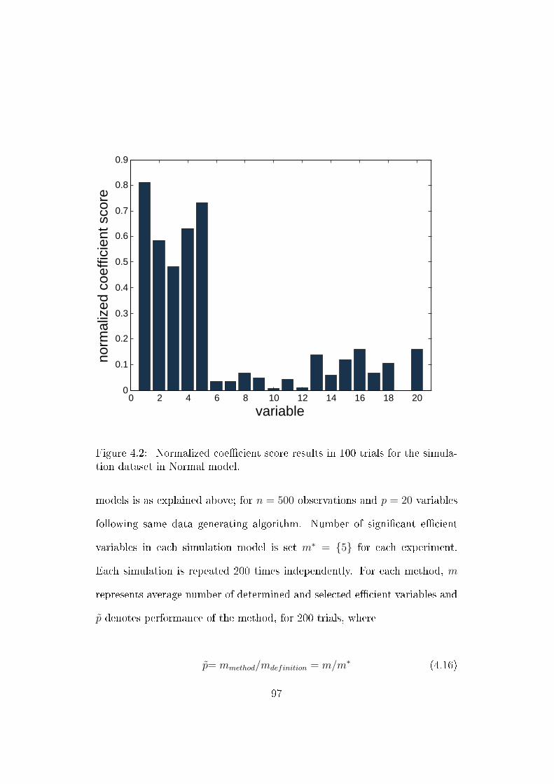
0 2 4 6 8 10 12 14 16 18 200

0.1

0.2

0.3

0.4

0.5

0.6

0.7

0.8

0.9

variable

norm

aliz

ed c

oeffi

cien

t sco

re

Figure 4.2: Normalized coecient score results in 100 trials for the simula-tion dataset in Normal model.

models is as explained above; for n = 500 observations and p = 20 variables

following same data generating algorithm. Number of signicant ecient

variables in each simulation model is set m∗ = 5 for each experiment.

Each simulation is repeated 200 times independently. For each method, m

represents average number of determined and selected ecient variables and

p denotes performance of the method, for 200 trials, where

p= mmethod/mdefinition = m/m∗ (4.16)

97

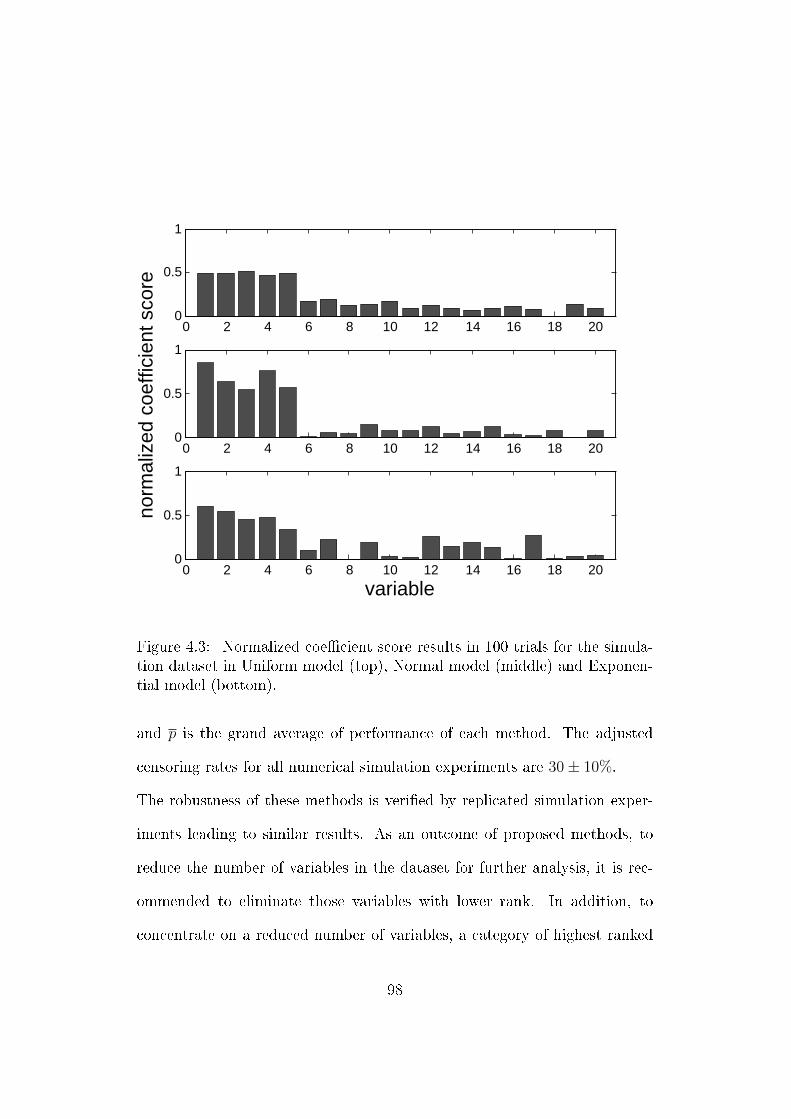
0 2 4 6 8 10 12 14 16 18 200

0.5

1

0 2 4 6 8 10 12 14 16 18 200

0.5

1

norm

aliz

ed c

oeffi

cien

t sco

re

0 2 4 6 8 10 12 14 16 18 200

0.5

1

variable

Figure 4.3: Normalized coecient score results in 100 trials for the simula-tion dataset in Uniform model (top), Normal model (middle) and Exponen-tial model (bottom).

and p is the grand average of performance of each method. The adjusted

censoring rates for all numerical simulation experiments are 30± 10%.

The robustness of these methods is veried by replicated simulation exper-

iments leading to similar results. As an outcome of proposed methods, to

reduce the number of variables in the dataset for further analysis, it is rec-

ommended to eliminate those variables with lower rank. In addition, to

concentrate on a reduced number of variables, a category of highest ranked

98

Table 4.2: Performance of the proposed methods based on three numericalsimulation experiments with 200 replications.

#1 #2 #3 AveMethod m p m p m p pRC 4.3 0.86 4.4 0.88 4.2 0.84 0.863R 4.0 0.80 4.2 0.84 3.9 0.78 0.81

Denition 5 5 5

variables is suggested.

99

Chapter 5

Methodology III: Hybrid

Clustering and Classication

Methods using Normalized

Weighted K-Mean

5.1 Overview

In continuation of analyzing the variable selection methods in complex high-

dimensional time-to-event data, a new approach is to cluster variables

into subsets in terms of similarity in order to reduce the number of variables

100

through (a) substitute a representative for each subset, and (b) determine

the most ecient or inecient subsets benecial to the process of variable

reduction. An ecient variables is dened in previous methodologies [50].

For that goal, two hybrid methods are proposed under the assumption that

the datasets includes uncensored data with no missing array.

The matrix A= [aij] has i rows and j columns while the column vector a= [aj]

has i elements. Also aij denotes the element of matrix A in row i and column

j, and the j'th column of matrix A is denoted by aj. Additionally, a large

matrix can be composed from smaller ones, such as A= [B C].

The original dataset contains time-to-event vector with n components, t= [tn]

and may include any type of explanatory variable in matrix U= [unp] which

includes n independent observations and p explanatory variables.

5.2 Methods and Algorithms for Variable Clus-

tering

Two methods are presented in this section:

101

5.2.1 Clustering through Cost Function

The outline of this method is to obtain the best possible clustering for vari-

ables through a hybrid heuristic algorithm by using k-mean method. In this

method the cumulative results from reasonable number of trials gives an opti-

mum solution which clusters variables considering the eciency on the event

time.

An original given dataset D as an entry of the algorithms is shown in Table

5.1.

Table 5.1: High-dimensional time-to-event dataset

Obs. # t u1 u2 u3 u4 u5 u6 . . . up

1 t1 u11 u12 u13 u14 u15 u16 . . . u1p

2 t2 u21 u22 u23 u24 u25 u26 . . . u2p

. . . . . . . . . . . . . . . . . . . . . . . . . . . . . .n tn un1 un2 un3 un4 un5 un6 . . . unp

The dataset in matrix D is dened as below, where t= [tn] is time-to-event

vector (time vector) and U= [uij] is variable matrix:

D= [t U] (5.1)

Also the variable matrix U with p vectors of n components is:

U=[u1 u2 . . . up] (5.2)

102

Procedure for each trial is dened as below:

Step 1: The variable matrix U is normalized in the rst step. Minimum and

maximum value of each element in vector uj for j = 1 . . . p are obtained as:

uminj = min uij , umaxj = max uij i = 1 . . . n (5.3)

Then normalized elements vij for all uij are calculated:

vij =uij − uminj

umaxj − uminji = 1 . . . n, j = 1 . . . p (5.4)

The result of the normalization is a n-by-p matrix V = [vnp] called normal-

ized variable matrix. The normalized dataset is presented by:

DN= [t V] =[t v1 v2 . . . vp] (5.5)

Step 2: In the normalized matrix V, vectors v1 to vp are clustered randomly

into q clusters containing k variable vectors in each cluster where k = dp/qe.

For instance, a set of 12 variables is clustered into 4 clusters of 3 variable

vectors. Each cluster including k variable vectors which randomly assigned

to a variable vectors of matrix V. Fig. 5.1 depicts the randomly clustering

sample in this step.

Therefore, in general, each of cluster is represented by 5.6 where k is number

of vector per cluster.

103

Variables

Obs.# 𝒕 𝒗𝟏 𝒗𝟐 𝒗𝟑 𝒗𝟒 𝒗𝟓 𝒗𝟔 … 𝒗𝒑

1 t1 v11 v12 v13 v14 u15 u16 … u1p 2 t2 v21 v22 v23 v24 u25 u26 … u2p … … … … … … … … … … n tn vn1 vn2 vn3 vn4 un5 un6 … unp

𝑾𝟏 𝑾𝟐 …

Figure 5.1: Randomly clustering process applies on matrix V.

Wj =[v1j v2

j . . . vkj

]j = 1 . . . q (5.6)

Superscripts in vectors show the members in each cluster and subscript de-

notes a cluster indicator. For example v23 is the second vector in the third

cluster and matrix W4 is the fourth cluster out of q cluster. Consequently

clustered dataset is presented in a new format:

DC=[t W1 W2 . . . Wq] (5.7)

Step 3: By dening transformation function (f), each cluster matrix Wj will

be substituted by a variable vector wj where i'th element of this vector is

resulted from applying transformation function on elements in i'th row in

the subject matrix Wj as below for i = 1 . . . n:

wij = f(v1ij, v

2ij, . . . , vkij) j = 1 . . . q (5.8)

This transformation is shown in Fig. 5.2:

104

𝒗𝟏 𝒗𝟐 𝒗𝟑 𝒘𝟏 v11 v12 v13 w11 v21 v22 v23 w21 … … … …

vn1 vn2 vn3 wn1

𝑾𝟏

Figure 5.2: Sample transformation.

In the rst level of calculation, transformation function is dened as an arith-

metic mean where for i = 1 . . . n:

wij = (v1ij + v2

ij + · · ·+ vkij)/k j = 1 . . . q (5.9)

For example, rst element of the second transformed vector when k = 3 is

w12 = (v112 + v2

12 + v312)/3 (5.10)

This process makes the transformed dataset in the form of

DR = [t W] =[t w1 w2 . . . wq] (5.11)

as a matrix which is constructed by q + 1 vectors.

Step 4: In this step k-mean clustering algorithm is applied by selecting pa-

rameter m as the desired number of the clusters. This process is performed

105

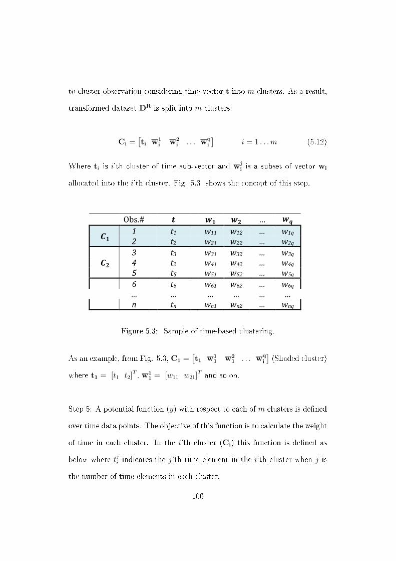
to cluster observation considering time vector t into m clusters. As a result,

transformed dataset DR is split into m clusters:

Ci =[ti w1

i w2i . . . wq

i

]i = 1 . . .m (5.12)

Where ti is i'th cluster of time sub-vector and wji is a subset of vector wi

allocated into the i'th cluster. Fig. 5.3 shows the concept of this step.

Obs.# 𝒕 𝒘𝟏 𝒘𝟐 … 𝒘𝒒

𝑪𝟏 1 t1 w11 w12 … w1q 2 t2 w21 w22 … w2q

𝑪𝟐 3 t3 w31 w32 … w3q 4 t2 w41 w42 … w4q 5 t5 w51 w52 … w5q

6 t6 w61 w62 … w6q … … … … … … n tn wn1 wn2 … wnq

Figure 5.3: Sample of time-based clustering.

As an example, from Fig. 5.3, C1 =[t1 w1

1 w21 . . . wq

i

](Shaded cluster)

where t1 = [t1 t2]T , w11 = [w11 w21]T and so on.

Step 5: A potential function (y) with respect to each of m clusters is dened

over time data points. The objective of this function is to calculate the weight

of time in each cluster. In the i'th cluster (Ci) this function is dened as

below where tji indicates the j'th time element in the i'th cluster when j is

the number of time elements in each cluster.

106

yi = y(t1i , t2i , . . . t

ji ) (5.13)

In the rst level we dene this function as an arithmetic mean of time data

points in each cluster, equal to yi.

Step 6: Cost function over a trial is dened to calculate aggregation of po-

tential functions output y′s for all clusters in a trial as a criterion to compare

all trials. The objective of this denition is to determine variance in the

output of the potential functions based on time-to-event. The formula for

cost function is following:

Cost =m−1∑i=1

m∑j=i+1

|yi − yj| (5.14)

For each trial, Steps 1 to 6 gives a cost result. Comparing all costs, the

greatest amount introduces the best k-mean clustering which is a function

of randomly clustered variables. Finally the variable clustering of mentioned

trial is selected as the optimum clustering.

5.2.2 Clustering through Weight Function

The concept and objective of this method is similar to the Method A. The

procedure of the Method B is following:

Step 1: The original dataset D includes time-to-event vector t= [tn] and

107

variable matrix U= [unp] (Equation 1). The time vector t and variable matrix

U are normalized similar to Step 1 in Method A. The result is a normalized

time vector t∗ = [t∗n] and a normalized variable matrix V = [vnp]. The new

dataset is:

D∗= [t∗ V] =[t∗ v1 v2 . . . vp] (5.15)

Step 2: Normalized dataset D∗ is split into m bins based on one of following

techniques in terms of vector t :

1. K-M Estimator: Based on survival time

2. Equal Bin: Based on equal time intervals

3. Equal Frequency: Based on the frequency

Fig. 5.4 represents clustering schema.

Obs.# 𝒕∗ 𝒗𝟏 𝒗𝟐 𝒗𝟑 𝒗𝟒 … 𝒗𝒑

𝑩𝟏 1 t*1 v11 v12 v13 v14 … v1p 2 t*2 v21 v22 v23 v24 … v2p

𝑩𝟐 3 t*3 v31 v32 v33 v34 … v3p 4 t*2 v41 v42 v43 v44 … v4p

5 t*5 v51 v52 v53 v54 … v5p … … … … … … … … n t*n vn1 vn2 vn3 vn4 … vnp

Figure 5.4: Schema of time-based binning.

108

Therefore,

Bi = [t∗i Vi] =[t∗i v1

i v2i . . . vp

i

]i = 1 . . .m (5.16)

Where t∗i is of time sub-vector in i'th bin and vji is a variable sub-vector of

vector vi allocated into the i'th bin. Vi is variable matrix including variable

elements in i'th bin (Bi) which is a sub-matrix of V. For instance, in the

shaded bin in Fig. 5.4, t∗2 = [t∗3, t∗4]T , v1

2 = [v31, v41]T .

As an example, let's assume a sample dataset of 9 observations (n = 9) in-

cluding time-to-event vector t = [10, 20, 30, 30, 50, 60, 70, 70, 90]T and

K-M survival function s = [1.00, 0.95, 0.80, 0.65, 0.55, 0.30, 0.25, 0.15, 0.00]T

as calculated, with respect to observations respectively. The results of bin-

ning into 3 bines (m = 3) bases on each of above techniques are presented in

Table 5.2:

Table 5.2: Sample of time-based binning based on three techniques.

K-M Estimator Equal Bin Equal FrequencyBin #1 1, 2, 3 1, 2, 3, 4 1, 2, 3Bin #2 4, 5 5, 6 4, 5, 6Bin #3 6, 7, 8, 9 7, 8, 9 7, 8, 9

Step 3: To calculate the weight of time in each cluster, weight function with

109

respect to each of m clusters is dened over time data points in each cluster.

This function in the rst level is dened as an arithmetic mean of time data

points in the cluster, zi. In Fig. 5.4, weight function of shaded bin #2 (B2)

including t∗3 and t∗4 is calculated as:

z2 = (t∗3 + t∗4)/2 (5.17)

Step 4: By multiplication each weight function result scalar (zi) in corre-

sponding bin variable matrix (Vi), weighted variable matrix V∗ is generated.

V∗i = ziVi i = 1 . . .m (5.18)

V∗T=[V∗T1 V∗T2 . . . V∗Tm

](5.19)

Step 5: Clustering algorithm k-mean applies on weighted variable matrix V∗

in terms of variables to cluster variable vectors in subsets.

5.3 Experiment and Result

Coding methods A and B by MATLAB shows robustness by tuning in pa-

rameter denition such as k and m.

A sample result for Method A applied on PBC dataset including 16 selected

110

variables and 111 uncensored observations are given in Table 5.3 for k = 4

and m = 5, for 100 trials:

Table 5.3: Clustering by cost function

Cluster # Variable #1 1, 2, 13, 152 3, 5, 7, 103 8, 9, 12, 144 4, 6, 11, 16

The result shows the four variable clusters obtained by cost function com-

parison.

111

Chapter 6

Conclusion

Capter 6 presents a summary of research and an overview for further

research steps.

6.1 Summary

Proper management and utilization of valuable data could signicantly in-

crease knowledge and reduce cost by preventive actions, whereas erroneous

and misinterpreted data could lead to poor inference and decision-making.

Variable selection is necessary in a decision-making application as unimpor-

tant variables adds unnecessary noise and often it is not clear which variables

would be most useful and cost-eective to collect. Therefore data collection

and analysis of data in data-driven decision-making plays crucial roles. In

112

many cases data are collected from dierent sources such as nancial reports

and marketing data, and they are combined for more informative decision-

making. Consequently, determining eective explanatory variables, speci-

cally in complex and high-dimensional data provides an excellent opportunity

to increase eciency and reduce costs. Unlike traditional datasets with few

explanatory variables, analysis of datasets with high number of variables re-

quires dierent approaches.

The proposed methods are benecial to explanatory variable selection in

decision-making process to obtain an appropriate subset of variables from

among a high-dimensional and large-scale time-to-event data. By using

such novel methods and reducing the number of variables, data analysis

and decision-making processes will be faster, simpler and more accurate. For

example, in business applications, many explanatory variables in a customer

survey are dened based on cause and eect analysis process data or simi-

lar analytic process outcome. In most cases, correlations of these variables

are complicated and unknown, and it is important to simply understand the

eciency of each variable in the survey. These procedures potentially are ap-

plicable solutions for many problems in a vast area of science and technology.

113

6.2 Next Steps

Next steps in this research are to examine the algorithms by exhaustive

method for robustness and use evolutionary algorithms to optimize the solu-

tion.

By denition, heuristic algorithms nd approximate solutions in acceptable

time and computational space. These algorithms either give nearly the right

answer or provide a solution not for all instances of the problem and usually

are used for problems that cannot be easily solved. An ecient heuristic

algorithm class is evolutionary algorithms which are methods that exploit

ideas of biological evolution, such as reproduction, mutation and recombi-

nation, for searching the solution of an optimization problem. They apply

the principle of survival on a set of potential solutions to produce gradual

approximations to the optimum. Evolutionary techniques can dier in the

details of implementation and the problems to which they are applied.

Also, the another challenge in this research is to face the data streaming cir-

cumstances in which variables are time-dependent where real-time analysis

of data is more complicated.

114

This is just the beginning ...

115

Bibliography

[1] Hervé Abdi and Lynne J Williams. Principal component analysis. Wiley

Interdisciplinary Reviews: Computational Statistics, 2(4):433459, 2010.

[2] D Addison, Stefan Wermter, and G Arevian. A comparison of fea-

ture extraction and selection techniques. In Proceedings of International

Conference on Articial Neural Networks (Supplementary Proceedings),

pages 212215, 2003.

[3] H Akaike. An information criterion (aic). Math Sci, 14(153):59, 1976.

[4] D.H. Bestereld. Total Quality Management. Prentice Hall, 1995.

[5] Leo Breiman, Jerome Friedman, Charles J Stone, and Richard A Olshen.

Classication and Regression Trees. CRC Press, 1984.

[6] Brad Brown, Michael Chui, and James Manyika. Are you ready for the

era of big data. McKinsey Quarterly, 4:2435, 2011.

[7] E Brynjolfsson. A revolution in decision-making improves productivity,

2012.

[8] Jonathan Buckley and Ian James. Linear regression with censored data.

Biometrika, 66(3):429436, 1979.

[9] Jerome R Busemeyer and James T Townsend. Decision eld theory: A

dynamic-cognitive approach to decision making in an uncertain environ-

ment. Psychological Review, 100(3):432, 1993.

116

[10] Junyi Chai, James NK Liu, and Eric WT Ngai. Application of decision-

making techniques in supplier selection: A systematic review of litera-

ture. Expert Systems with Applications, 40(10):38723885, 2013.

[11] David R Cox. Regression models and life-tables. Journal of the Royal

Statistical Society. Series B (Methodological), pages 187220, 1972.

[12] Nasser Fard and Keivan Sadeghzadeh. Heuristic ranking classication

method for complex large-scale survival data. In Modelling, Compu-

tation and Optimization in Information Systems and Management Sci-

ences, pages 4756. Springer, 2015.

[13] Dan Feldman, Melanie Schmidt, and Christian Sohler. Turning big data

into tiny data: Constant-size coresets for k-means, pca and projective

clustering. In Proceedings of the Twenty-Fourth Annual ACM-SIAM

Symposium on Discrete Algorithms, pages 14341453. SIAM, 2013.

[14] Thomas A Feo and Mauricio GC Resende. Greedy randomized adaptive

search procedures. Journal of global optimization, 6(2):109133, 1995.

[15] Gartner. 2011.

[16] David A Garvin. Competing on the eight dimensions of quality. IEEE

Engineering Management Review, 24(1):1523, 1996.

[17] Michel Gendreau and Jean-Yves Potvin. Tabu search. In Search Method-

ologies, pages 165186. Springer, 2005.

[18] Jan J Gerbrands. On the relationships between svd, klt and pca. Pattern

Recognition, 14(1):375381, 1981.

[19] Isabelle Guyon and André Elissee. An introduction to variable and

feature selection. The Journal of Machine Learning Research, 3:1157

1182, 2003.

[20] J Pirie Hart and Andrew W Shogan. Semi-greedy heuristics: An empir-

ical study. Operations Research Letters, 6(3):107114, 1987.

117

[21] Joe Hellerstein. Parallel programming in the age of big data. Gigaom

Blog, 2008.

[22] Martin Hilbert and Priscila López. The world's technological capacity to

store, communicate, and compute information. science, 332(6025):60

65, 2011.

[23] Theodore R Holford et al.Multivariate Methods in Epidemiology. Oxford

University Press, 2002.

[24] Jian Huang, Shuangge Ma, and Huiliang Xie. Regularized estimation

in the accelerated failure time model with high-dimensional covariates.

Biometrics, 62(3):813820, 2006.

[25] IBM. Information integration and governance. 2011.

[26] IBM. What is big data? bringing big data to the enterprise. 2013.

[27] Hemant Ishwaran, Udaya B Kogalur, Eugene H Blackstone, and

Michael S Lauer. Random survival forests. The Annals of Applied Statis-

tics, pages 841860, 2008.

[28] I. Ishwaran and U.B. Kogalur. Random survival forests for R. 2007.

[29] Zhezhen Jin, DY Lin, and Zhiliang Ying. On least-squares regression

with censored data. Biometrika, 93(1):147161, 2006.

[30] Ian Jollie. Principal Component Analysis. Wiley Online Library, 2002.

[31] John D Kalbeisch and Ross L Prentice. The Statistical Analysis of

Failure Time Data, volume 360. John Wiley & Sons, 2011.

[32] Louis-Philippe Kronek and Anupama Reddy. Logical analysis of survival

data: prognostic survival models by detecting high-degree interactions

in right-censored data. Bioinformatics, 24(16):i248i253, 2008.

[33] Elisa T Lee and John Wang. Statistical Methods for Survival Data Anal-

ysis, volume 476. John Wiley & Sons, 2003.

118

[34] Huan Liu, Farhad Hussain, Chew Lim Tan, and Manoranjan Dash. Dis-

cretization: An enabling technique. Data Mining and Knowledge Dis-

covery, 6(4):393423, 2002.

[35] Steve Lohr. The age of big data. New York Times, 11, 2012.

[36] Shuangge Ma, Michael R Kosorok, and Jason P Fine. Additive risk

models for survival data with high-dimensional covariates. Biometrics,

62(1):202210, 2006.

[37] James Manyika, Michael Chui, Brad Brown, Jacques Bughin, Richard

Dobbs, Charles Roxburgh, and Angela H Byers. Big data: The next

frontier for innovation, competition, and productivity. 2011.

[38] C. Matteo and G. Francesca. Variable selection methods: An introduc-

tion.

[39] Andrew McAfee, Erik Brynjolfsson, Thomas H Davenport, DJ Patil,

and Dominic Barton. Big data. The management revolution. Harvard

Business Review, 90(10):6167, 2012.

[40] Alexandre C Mendes and Nasser Fard. Accelerated failure time models

comparison to the proportional hazard model for time-dependent covari-

ates with recurring events. International Journal of Reliability, Quality

and Safety Engineering, 21(02):1450010, 2014.

[41] J Moran. Is big data a big problem for manufacturers, 2013.

[42] Hiroshi Motoda and Huan Liu. Feature selection, extraction and con-

struction. Communication of IICM (Institute of Information and Com-

puting Machinery, Taiwan), 5:6772, 2002.

[43] M. Nemscho. How big data can improve manufacturing quality, 2014.

[44] Arthur V Peterson Jr. Expressing the kaplan-meier estimator as a func-

tion of empirical subsurvival functions. Journal of the American Statis-

tical Association, 72(360a):854858, 1977.

119

[45] Philip Russom et al. Big data analytics. TDWI Best Practices Report,

Fourth Quarter, 2011.

[46] Keivan Sadeghzadeh and Nasser Fard. Multidisciplinary decision-

making approach to high-dimensional event history analysis through

variable reduction. European Journal of Economics and Management,

1(2):7689, 2014.

[47] Keivan Sadeghzadeh and Nasser Fard. Nonparametric data reduction

approach for large-scale survival data analysis. In Reliability and Main-

tainability Symposium (RAMS), 2015 Annual, pages 16. IEEE, 2015.

[48] Keivan Sadeghzadeh and Nasser Fard. Variable selection methods

for right-censored time-to-event data with high-dimensional covariates.

Journal of Quality and Reliability Engineering, 2015, 2015.

[49] Keivan Sadeghzadeh and Nasser Fard. Complex data classication in

weighted accelerated failure time model. IEEE, In Press.

[50] Keivan Sadeghzadeh, Nasser Fard, and Mohammad Bagher Salehi. An-

alytical clustering procedures in massive failure data. Applied Stochastic

Models in Business and Industry, In Press.

[51] Keivan Sadeghzadeh and Mohammad Bagher Salehi. Mathematical

analysis of fuel cell strategic technologies development solutions in

the automotive industry by the topsis multi-criteria decision making

method. International Journal of Hydrogen Energy, 36(20):1327213280,

2011.

[52] Yvan Saeys, Iñaki Inza, and Pedro Larrañaga. A review of feature

selection techniques in bioinformatics. bioinformatics. Bioinformatics,

23(19):25072517, 2007.

[53] Gideon Schwarz et al. Estimating the dimension of a model. The Annals

of Statistics, 6(2):461464, 1978.

120

[54] Toby Segaran and Je Hammerbacher. Beautiful Data: The Stories

Behind Elegant Data Solutions. " O'Reilly Media, Inc.", 2009.

[55] Winfried Stute and J-L Wang. The strong law under random censorship.

The Annals of Statistics, pages 15911607, 1993.

[56] KP Suresh. An overview of randomization techniques: An unbiased as-

sessment of outcome in clinical research. Journal of Human Reproductive

Sciences, 4(1):8, 2011.

[57] P. Tan. Introduction to Data Mining. WP Co, 2006.

[58] A.R. Tenner and I.J. Detoro. Total Quality Management: Three Steps

to Continuous Improvement. Addison-Wesley.

[59] Hosmer D. W., Jr. and S. Lemeshow. Applied Survival Analysis: Re-

gression Modeling of Time to Event Data. Wiley, 1999.

[60] Fang Yao. Functional principal component analysis for longitudinal and

survival data. Statistica Sinica, 17(3):965, 2007.

[61] J. Ye. Unsupervised and Supervised Dimension Reduction: Algorithms

and Connections. Arizona State University.

[62] Donglin Zeng and DY Lin. Ecient estimation for the accelerated

failure time model. Journal of the American Statistical Association,

102(480):13871396, 2007.

[63] William R Zwick and Wayne F Velicer. Comparison of ve rules for

determining the number of components to retain. Psychological Bulletin,

99(3):432, 1986.

121

Appendices

122

Appendix A

Matlab Code

1 clc;2 clear;3 close all;4 commandwindow;5

6 %% ...========================================================================

7 %% part setting8 % ...

=========================================================================9 %%

10 % part 01: sda (survival data analysis)11 % part 02: svd (singular value decomposition)12 % part 03: pca (principal component analysis)13 % part 04: cox phm (cox proportional hazards model)14 % part 05: mlr (multiple linear regression model)15 % part 06: k-means (clustering)16 % part 07: rf (random forest)17 % part 08: on and off comparison (doe approach)18 % part 09: test score - brute-force (exhaustive) search (sda ...

combination)19 % part 10: test score - random subset selection (sda ...

randomization)20 % part 11: time score - brute-force (exhaustive) search (sda ...

combination)21 % part 12: time score - random subset selection (sda ...

randomization)22 % part 13: bisection semi-greedy clustering algorithm ...

(bisection method)23 % part 14: splitting semi-greedy clustering algorithm ...

(splitting method)

123

24 % part 15: weighted standardized score method25 % part 16: aft26 % part 17: penalty - cost function27 % part 18: hybrid algorithm28 % part 19: variable clustering and correlation29 % part 20: plots and charts30 % part 21: fuzzy time score - random subset selection31 % part 22: fuzzy weighted standardized score method32 % part 23: MIII133 % part 24: MIII234 % part no.: [01 02 03 04 05 06 07 08 09 10 11 12 13 14 15 16 ...

17 18 19 20 21 22 23 24]35 part_code = [ 0 0 0 0 0 0 0 0 0 0 0 0 0 0 0 0 ...

0 0 0 0 0 0 0 0];36

37 %% ...========================================================================

38 %% data setting39 % ...

=========================================================================40 %%41 % data 01: data generator 0142 % data 02: data generator 0243 % data 03: data generator 0344 % data 04: pbc data45 % data 05: pharynx data46 % data 06: actg data47 % data 07: new data48 % data 08: gbcs data49 % data 09: va data50 % data 10: sample data51 % data 11: simulation data generator 0152 % data 12: simulation data generator 0253 % data 13: simulation data generator 0254 % data 14: sample data55 % data no.: [01 02 03 04 05 06 07 08 09 10 11 12 13 14]56 data_code = [ 0 0 0 1 0 0 0 0 0 0 0 0 0 0];57

58 % http://vincentarelbundock.github.io/Rdatasets/datasets.html59

60 %% ...========================================================================

61 %% censoring62 % ...

=========================================================================63 %%64 % data censoring 01: uncensored65 % data censoring 02: censored66 % data cens no.: [01 02]

124

67 data_cens_code = [ 1 1];68

69 %% ...========================================================================

70 %% explanatory variable data type71 % ...

=========================================================================72 %%73 % data type 01: logical74 % data type 02: normal75 % data type no.: [01 02]76 data_type_code = [ 1 1];77

78 %% ...========================================================================

79 %% calculation method80 % ...

=========================================================================81 %%82 % method 01: mid-range83 % method 02: mean84 % method 03: median85 % method 04:86 % method no.: [01 02 03 04]87 method_code = [ 1 0 0 0];88

89 %% ...========================================================================

90 %% ---------- data 01: data generator 01 ...----------------------------------

91 % ...=========================================================================

92 %%93 if data_code(01) == 194

95 data = [];96

97 data_generated = rand(100,10);98

99 x_km_all = rand(418,17);100 data = [data,pbc(:,1:3),x_km_all];101

102 end % if data_code(01) == 1103

104 %% ...========================================================================

105 %% ---------- data 02: data generator 02 ...----------------------------------

106 % ...

125

=========================================================================107 %%108 if data_code(02) == 1109

110 data = [];111 n = 400;112 lower = 1;113 upper = 5;114

115 data(1:n,1) = 1:n;116 % data(1:n,2) = sortrows(fix(1000*rand(n,1)));117 data(1:100,2) = sortrows(fix(100*rand(100,1)));118 data(101:200,2) = sortrows(fix(100*rand(100,1)+200));119 data(201:300,2) = sortrows(fix(100*rand(100,1)+400));120 data(301:400,2) = sortrows(fix(100*rand(100,1)+600));121

122 data(1:n,3) = 1;123

124 data(1:n,4) = 0; % data(n,4) = 0.1;125 data(1:n,5) = 1; % data(n,4) = 0.9;126 data(1:n,6) = 2*data(1:n,1) + 2*rand(n,1); % a(ID) + e127 data(1:n,7) = -3*data(1:n,1) + -3*rand(n,1); % a(ID)^2 + e128 data(1:n,8) = 4*data(1:n,2) + 4*rand(n,1); % a(T) + e129 data(1:n,9) = -5*data(1:n,2) + -5*rand(n,1); % a(T)^2 + e130 data(1:n,10) = sign(mod((data(1:n,1)-1 - ...

mod(data(1:n,1)-1,5)),10)); % 0 and 1 in order for ...every 5 cons. obs.

131 data(1:n,11) = randn(n,1); % normal random N(0,1)132 data(1:n,12) = 1 + 2.*randn(n,1); % normal random N(0,1)133 data(1:n,13) = normrnd(0,1,n,1); % normal random N(0,1)134 data(1:n,14) = randi([lower upper],n,1); % integer ...

uniform random (1 to upper)135 data(1:n,15) = lower + (upper-lower).*rand(n,1); % ...

uniform random (lower to upper)136 data(1:n,16) = rand(n,1); % uniform random (0 to 1)137 data(1:n,17) = rand(n,1)≤0.1; % 0 for 90% and 1 for 10%138 data(1:n,18) = rand(n,1)≤0.5; % 0 for 50% and 1 for 50%139 data(1:n,19) = rand(n,1)≤0.9; % 0 for 10% and 1 for 90%140 data(1:n,20) = random('unif',1,10,n,1); % uniform random ...

U(2)141 data(1:n,21) = random('norm',2,3,n,1); % normal random ...

N(2,3)142 data(1:n,22) = random('exp',2,n,1); % exponential random ...

E(2)143 data(1:n,23) = random('wbl',2,3,n,1); % weibull random ...

W(2,3)144

145 % http://www.mathworks.com/help/stats/random.html146

126

147 end % if data_code(02) == 1148

149 %% ...========================================================================

150 %% ---------- data 03: data generator 03 ...----------------------------------

151 % ...=========================================================================

152 %%153 if data_code(03) == 1154

155 data = [];156 n = 300;157 lower = 1;158 upper = 5;159

160 data(1:n,1) = 1:300;161 % data(1:n,2) = sortrows(fix(1000*rand(n,1)));162 data(1:100,2) = sortrows(fix(100*rand(100,1)));163 data(101:200,2) = sortrows(fix(100*rand(100,1)+200));164 data(201:300,2) = sortrows(fix(100*rand(100,1)+400));165

166 data(1:n,3) = 1;167

168 data(1:n,4) = 0; % data(n,4) = 0.1;169 data(1:n,5) = 1; % data(n,4) = 0.9;170 data(1:n,6) = 2*data(1:n,1) + 2*rand(n,1); % a(ID) + e171 data(1:n,7) = -3*data(1:n,1) + -3*rand(n,1); % a(ID)^2 + e172 data(1:n,8) = 4*data(1:n,2) + 4*rand(n,1); % a(T) + e173 data(1:n,9) = -5*data(1:n,2) + -5*rand(n,1); % a(T)^2 + e174 data(1:n,10) = sign(mod((data(1:n,1)-1 - ...

mod(data(1:n,1)-1,5)),10)); % 0 and 1 in order for ...every 5 cons. obs.

175 data(1:n,11) = randn(n,1); % normal random N(0,1)176 data(1:n,12) = 1 + 2.*randn(n,1); % normal random N(0,1)177 data(1:n,13) = normrnd(0,1,n,1); % normal random N(0,1)178 data(1:n,14) = randi([lower upper],n,1); % integer ...

uniform random (1 to upper)179 data(1:n,15) = lower + (upper-lower).*rand(n,1); % ...

uniform random (lower to upper)180 data(1:n,16) = rand(n,1); % uniform random (0 to 1)181 data(1:n,17) = rand(n,1)≤0.1; % 0 for 90% and 1 for 10%182 data(1:n,18) = rand(n,1)≤0.5; % 0 for 50% and 1 for 50%183 data(1:n,19) = rand(n,1)≤0.9; % 0 for 10% and 1 for 90%184 data(1:n,20) = random('unif',1,10,n,1); % uniform random ...

U(2)185 data(1:n,21) = random('norm',2,3,n,1); % normal random ...

N(2,3)186 data(1:n,22) = random('exp',2,n,1); % exponential random ...

127

E(2)187 data(1:n,23) = random('wbl',2,3,n,1); % weibull random ...

W(2,3)188

189 % http://www.mathworks.com/help/stats/random.html190

191 end % if data_code(03) == 1192

193 %% ...========================================================================

194 %% ---------- data 04: pbc data ...-------------------------------------------

195 % ...=========================================================================

196 %%197 if data_code(04) == 1198

199 load 'pbc';200

201 data = pbc;202

203 % N Case number.204 % X The number of days between registration and the ...

earlier of death,liver transplantation,or study ...analysis time in July,1986.

205 % D 1 if X is time to death,0 if time to censoring206

207 % Z1 Treatment Code,1 = D-penicillamine,2 = placebo.208 % Z2 Age in years. For the first 312 cases,age was ...

calculated by209 % dividing the number of days between birth and ...

study registration by 365.210 % Z3 Sex,0 = male,1 = female.211 % Z4 Presence of ascites,0 = no,1 = yes.212 % Z5 Presence of hepatomegaly,0 = no,1 = yes.213 % Z6 Presence of spiders 0 = no,1 = Yes.214 % Z7 Presence of edema,0 = no edema and no diuretic ...

therapy for edema; 0.5 = edema present for which no ...diuretic therapy was given,or

215 % edema resolved with diuretic therapy; 1 = edema ...despite diuretic therapy

216 % Z8 Serum bilirubin,in mg/dl.217 % Z9 Serum cholesterol,in mg/dl.218 % Z10 Albumin,in gm/dl.219 % Z11 Urine copper,in mg/day.220 % Z12 Alkaline phosphatase,in U/liter.221 % Z13 SGOT,in U/ml.222 % Z14 Triglycerides,in mg/dl.223 % Z15 Platelet count; coded value is number of ...

128

platelets per-cubic-milliliter of blood divided by 1000.224 % Z16 Prothrombin time,in seconds.225 % Z17 Histologic stage of disease,graded 1,2,3,or 4.226

227 end % if data_code(04) == 1228

229 %% ...========================================================================

230 %% ---------- data 05: pharynx data ...------------------------------------------

231 % ...=========================================================================

232 %%233 if data_code(05) == 1234

235 load 'pharynx';236

237 data = pharynx;238

239 % CASE Case Number240 % TIME Survival time in days from day of diagnosis241 % STATUS 0=censored, 1=dead242 % INST Participating Institution243 % SEX 1=male, 2=female244 % TX Treatment: 1=standard, 2=test245 % GRADE 1=well differentiated, 2=moderately ...

differentiated, 3=poorly differentiated, 9=missing246 % AGE In years at time of diagnosis247 % COND Condition: 1=no disability, 2=restricted ...

work, 3=requires assistance with self care, 4=bed ...confined, 9=missing

248 % SITE 1=faucial arch, 2=tonsillar fossa, ...3=posterior pillar, 4=pharyngeal tongue, 5=posterior wall

249 % T_STAGE 1=primary tumor measuring 2 cm or less in ...largest diameter, 2=primary tumor measuring 2 cm to 4 ...cm in largest diameter with

250 % minimal infiltration in depth, 3=primary ...tumor measuring more than 4 cm, 4=massive invasive tumo

251 % N_STAGE 0=no clinical evidence of node metastases, ...1=single positive node 3 cm or less in diameter, not ...fixed, 2=single positive

252 % node more than 3 cm in diameter, not fixed, ...3=multiple positive nodes or fixed positive nodes

253 % ENTRY_DT Date of study entry: Day of year and year, dddyy254

255 end % if data_code(05) == 1256

257 %% ...========================================================================

129

258 %% ---------- data 06: actg data ...------------------------------------------

259 % ...=========================================================================

260 %%261 if data_code(06) == 1262

263 load 'actg';264

265 data = actg;266

267 end % if data_code(06) == 1268

269 %% ...========================================================================

270 %% ---------- data 07: new data ...-------------------------------------------

271 % ...=========================================================================

272 %%273 if data_code(07) == 1274

275 load 'new';276

277 data = gbcs;278

279 end % if data_code(07) == 1280

281 %% ...========================================================================

282 %% ---------- data 08: gbcs data ...------------------------------------------

283 % ...=========================================================================

284 %%285 if data_code(08) == 1286

287 load 'gbcs';288

289 data = gbcs;290

291 end % if data_code(08) == 1292

293 %% ...========================================================================

294 %% ---------- data 09: va data ...--------------------------------------------

295 % ...=========================================================================

130

296 %%297 if data_code(07) == 1298

299 load 'va';300

301 data = va;302

303 end % if data_code(09) == 1304

305 %% ...========================================================================

306 %% ---------- data 10: sample data ...----------------------------------------

307 % ...=========================================================================

308 %%309 if data_code(10) == 1310

311 load 'sample01';312 load 'sample02';313 load 'sample03';314 load 'sample04';315 load 'sample05';316

317 data = sample05;318

319 end % if data_code(10) == 1320

321 %% ---------- data 11: simulation data generator 01 ...-----------------------

322 % ...=========================================================================

323 %%324 if data_code(11) == 1325

326 data = [];327 n = 1000;328 lower = 1;329 upper = 5;330

331 data(1:n,1) = 1:1000;332 % data(1:n,2) = sortrows(fix(1000*rand(n,1)));333

334 data(1:n,3) = 1;335

336 data(1:n,4) = normrnd(0,1,n,1) %+ data(1:n,1); % normal ...random N(0,1)

337 data(1:n,5) = normrnd(0,1,n,1) %+ data(1:n,1); % normal ...random N(0,1)

131

338 data(1:n,6) = normrnd(0,1,n,1) %+ data(1:n,1); % normal ...random N(0,1)

339 data(1:n,7) = normrnd(0,1,n,1) %+ data(1:n,1); % normal ...random N(0,1)

340 data(1:n,8) = normrnd(0,1,n,1) %+ data(1:n,1); % normal ...random N(0,1)

341 data(1:n,9) = normrnd(0,1,n,1) % normal random N(0,1)342 data(1:n,10) = normrnd(0,1,n,1) % normal random N(0,1)343 data(1:n,11) = normrnd(0,1,n,1) % normal random N(0,1)344 data(1:n,12) = normrnd(0,1,n,1) % normal random N(0,1)345 data(1:n,13) = normrnd(0,1,n,1) % normal random N(0,1)346 data(1:n,14) = rand(n,1); % uniform random (0 to 1)347 data(1:n,15) = rand(n,1); % uniform random (0 to 1)348 data(1:n,16) = rand(n,1); % uniform random (0 to 1)349 data(1:n,17) = rand(n,1); % uniform random (0 to 1)350 data(1:n,18) = rand(n,1); % uniform random (0 to 1)351 data(1:n,19) = random('exp',1,n,1); % exp random (1)352 data(1:n,20) = random('exp',1,n,1); % exp random (1)353 data(1:n,21) = random('exp',1,n,1); % exp random (1)354 data(1:n,22) = random('exp',1,n,1); % exp random (1)355 data(1:n,23) = random('exp',1,n,1); % exp random (1)356 data(1:n,24) = random('wbl',2,1,n,1); % exp random (2)357 data(1:n,25) = random('wbl',2,1,n,1); % exp random (2)358 data(1:n,26) = random('wbl',2,1,n,1); % exp random (2)359 data(1:n,27) = random('wbl',2,1,n,1); % exp random (2)360 data(1:n,28) = random('wbl',2,1,n,1); % exp random (2)361

362 for i=1:n363 betha1x = sum(data(i,4:8));364 betha2x = sum(data(i,9:13));365 betha3x = sum(data(i,14:18));366 betha4x = sum(data(i,19:28));367 data(i,2) = 10*betha1x + 1*betha2x + 0.1*betha3x + ...

0*betha4x;368 end369

370 % http://www.mathworks.com/help/stats/random.html371

372 end % if data_code(11) == 1373

374 %% ...========================================================================

375 %% ---------- data 12: simulation data generator 02 ...-----------------------

376 % ...=========================================================================

377 %%378 if data_code(12) == 1379

132

380 data = [];381 n = 1000;382 lower = 1;383 upper = 5;384

385 data(1:n,1) = 1:1000;386 % data(1:n,2) = sortrows(fix(1000*rand(n,1)));387

388 data(1:n,3) = 1;389

390 for i = 4:23391 data(1:n,i) = normrnd(0,1,n,1); % normal random N(0,1)392 % data(1:n,i) = rand(n,1); % uniform random (0 to 1)393 % data(1:n,i) = random('exp',1,n,1); % ex;p random (1)394 % data(1:n,i) = random('wbl',2,1,n,1); % exp random (2)395 end396

397 % data(1:n,i) = rand(n,1); % uniform random (0 to 1)398 % data(1:n,i) = random('exp',1,n,1); % exp random (1)399 % data(1:n,i) = random('wbl',2,1,n,1); % exp random (2)400

401

402 for i = 1:n403 betha1x = sum(data(i,4:8));404 betha2x = sum(data(i,9:13));405 betha3x = sum(data(i,14:18));406 betha4x = sum(data(i,19:23));407 % betha4x = sum(data(i,19:28));408 data(i,2) = 10*betha1x + 1*betha2x + 0.1*betha3x + ...

0*betha4x;409 end410

411 % http://www.mathworks.com/help/stats/random.html412

413 end % if data_code(12) == 1414

415 %% ...========================================================================

416 %% ---------- data 13: simulation data generator 03 ...-----------------------

417 % ...=========================================================================

418 %%419 if data_code(13) == 1420

421 end % if data_code(13) == 1422

423 %% ...========================================================================

133

424 %% ---------- data 14: data generator 02 ...----------------------------------

425 % ...=========================================================================

426 %%427 if data_code(14) == 1428

429 data = [];430

431 data_generated = rand(100,10);432

433 x_km_all = rand(418,17);434 data = [data,pbc(:,1:3),x_km_all];435

436 end % if data_code(14) == 1437

438 %%439 %% ...

========================================================================440 %% general setting441 % ...

=========================================================================442 %%443 data(any(isnan(data),2),:)=[]; % remove NaN data [data cleaning]444

445 data_unc = data; % defining uncensored dataset matrix446 data_unc(find(data_unc(:,3)==0),:) = []; % remove censored data447 data_unc = sortrows(data_unc,2); % sort by failure time448

449 data_cens = data; % defining censored dataset matrix450 data_cens = sortrows(data_cens,2); % sort by failure time451

452 if data_cens_code(01) == 1453 [n p] = size(data_unc);454 data_cal = data_unc; % defining calculate dataset matrix455 end456

457 if data_cens_code(02) == 1458 [n p] = size(data_cens);459 data_cal = data_cens; % defining calculate dataset matrix460 end461

462 data_cal(n+1,:) = min(data_cal(1:n,:)); % calculate variable min463 data_cal(n+2,:) = max(data_cal(1:n,:)); % calculate variable max464

465 if method_code(01) == 1; data_cal(n+3,:) = (data_cal(n+1,:) ...+ data_cal(n+2,:))/2; end % calculate variable "mid-range"

466 if method_code(02) == 1; data_cal(n+3,:) = ...mean(data_cal(1:n,:)); end; % calculate variable "mean"

134

467 if method_code(03) == 1; data_cal(n+3,:) = ...median(data_cal(1:n,:)); end; % calculate variable "median"

468

469 data_raw = data_cal(1:n,4:p); % defining raw dataset matrix470 data_nor = zscore(data_raw); % defining normalized dataset ...

matrix471

472 % logical vector473

474 data_log = data_cal; % defining logical dataset matrix475 data_fuz = data_cal; % defining logical dataset matrix476

477 for i = 1:n478 for j = 4:p479 if data_log(i,j) < data_log(n+3,j);480 data_log(i,j) = 0;481 else482 data_log(i,j) = 1;483 end484 end485 end486

487 for i = 1:n488 for j = 4:p489 if data_fuz(n+1,j)== data_fuz(n+2,j);490 data_fuz(i,j) = data_fuz(n+1,j);491 else492 data_fuz(i,j) = ...

(data_fuz(i,j)-data_fuz(n+1,j))/(data_fuz(n+2,j)-data_fuz(n+1,j));493 end494 end495 end496

497 if data_type_code(01) == 1498 data_time = data_log(1:n,2); % defining failure time vector499 data_var = data_log(1:n,4:p); % defining logical ...

variable dataset matrix500 end501

502 if data_type_code(02) == 1503 data_time = data_fuz(1:n,2); % defining failure time vector504 % data_var = data_fuz(1:n,4:p); % defining logical ...

variable dataset matrix505 data_fuzzy = data_fuz(1:n,4:p); % defining logical ...

variable dataset matrix506 end507

508 % extra change for var 1 (switching) % data_var(:,1) = ...sign(data_var(:,1)-1);

135

509

510 var(p-3) = ...struct('all',[],'one',[],'zero',[],'failure',[],'surv',[]);

511

512 for i = 1:p-3513 [var(i).all(:,1)] = data_log(1:n,2); % time514 [var(i).all(:,2)] = data_log(1:n,3); % status515 [var(i).all(:,3)] = data_log(1:n,i+3); % variable (0 or 1)516

517 [var(i).one(:,1)] = data_log(1:n,2); % time518 [var(i).one(:,2)] = data_log(1:n,3); % status519 [var(i).one(:,3)] = data_log(1:n,i+3); % variable (only 1)520 var(i).one(find([var(i).one(1:end-1,3)]==0),:) = []; % ...

compeleting var(i).one (eleminating 0s)521 var_one_sum(i,1) = sum(var(i).one(:,1)); % cumulative time522 var_one_sum(i,2) = sum(var(i).one(:,1)); % cumulative ones523

524 [var(i).zero(:,1)] = data_log(1:n,2); % time525 [var(i).zero(:,2)] = data_log(1:n,3); % status526 [var(i).zero(:,3)] = data_log(1:n,i+3); % variable (only 0)527 var(i).zero(find([var(i).zero(1:end-1,3)]==1),:) = []; % ...

compeleting var(i).zero (eleminating 1s)528 var_zero_sum(i,1) = sum(var(i).zero(:,1)); % cumulative time529 var_zero_sum(i,2) = sum(var(i).zero(:,3)); % cumulative ...

zeros530

531 % [var(i).failure(:,1),var(i).failure(:,2)] = ...ecdf(var(i).one(:,1));

532 [var(i).failure(:,1),var(i).failure(:,2)] = ...ecdf(var(i).one(:,1),'censoring',var(i).one(:,2));

533 var(i).surv(:,1) = 1 - var(i).failure(:,1); % survival ...function for single variable #i

534 end535

536 % data_var_num = data_var;537 data_var_num = data_fuzzy;538 for i = 1:p-3539 data_var_num(n+1,i) = i;540 end541

542 %% model validation - Comparison of covariate correlations ...in the original and the transformed dataset

543

544 corrcoef_raw = corrcoef(data_raw); % ...++++++++++++++++++++++++++++++++++++++

545 corrcoef_var = corrcoef(data_var); % ...++++++++++++++++++++++++++++++++++++++

546

547 % corrplot(data_raw) % ...

136

++++++++++++++++++++++++++++++++++++++++++++++++++++548 % corrplot(data_var) % ...

++++++++++++++++++++++++++++++++++++++++++++++++++++549

550 x_cor = [];551 y_cor = [];552 z_cor = [];553

554 for i = 1:p-3555 scatter(corrcoef_raw(i,i+1:end),corrcoef_var(i,i+1:end),'k');556 x_cor = [x_cor, corrcoef_raw(i,i+1:end)];557 y_cor = [y_cor, corrcoef_var(i,i+1:end)];558 hold on; grid on;559 end560 [p_cor,s_cor] = polyfit(x_cor,y_cor,1); % poly fit561 z_cor = polyval(p_cor,x_cor);562 plot(x_cor,z_cor,'--','Color',[0.5 0.5 0.5]);563 hold on; grid on;564 xlabel('original dataset','FontSize',15); ...

ylabel('transformed dataset','FontSize',15); hold on565 axis([-.6 .6 -.6 .6]);566 axis square;567

568 x_axis = [1:p-3];569

570 %% ...========================================================================

571 %% ...========================================================================

572 %% ...========================================================================

573 %% ...========================================================================

574 %% ---------- parts ...-------------------------------------------------------

575 % ...=========================================================================

576

577 %% ...========================================================================

578 %% ---------- part 01: sda (survival data analysis) ...-----------------------

579 % ...=========================================================================

580 %%581 if part_code(01) == 1582

583 % ...http://www.mathworks.com/help/stats/kaplan-meier-methods.html

137

584 % ...http://www.mathworks.com/help/stats/examples/analyzing-survival-or-reliability-data.html

585

586 % The Wilcoxon rank sum test is equivalent to the ...Mann-Whitney U test.

587

588 % [P,H] = ranksum(...) returns the result of the ...hypothesis test, performed at the 0.05 significance ...level, in H.

589 % H=0 indicates that the null hypothesis ("medians are ...equal") cannot be rejected at the 5% level.

590 % H=1 indicates that the null hypothesis can be rejected ...at the 5% level.

591

592 % y = data_unc(:,2)'; % or data_time'593 y_data = data_cens(:,2)'; % or data_time'594 % freqy = data_unc(:,3)';595 censy = data_cens(:,3)';596 freqy = censy;597 % [f,x] = ecdf(y,'frequency',freqy);598 % [f_data,x_data] = ...

ecdf(y_data,'frequency',freqy,'function','survivor');599 [f_data,x_data] = ...

ecdf(y_data,'censoring',censy,'function','survivor');600 data_surv = f_data;601 % data_time = f_data;602

603 figure;604 % ecdf(y_data,'frequency',freqy,'function','survivor'); ...

% kaplan-meier plot605 ecdf(y_data,'censoring',censy,'function','survivor'); % ...

kaplan-meier plot606 hold on; grid on;607 title('kaplan-meier survival function','FontSize',15);608 xlabel('time,t','FontSize',15); ylabel('survival ...

probability,s(t)','FontSize',15);609 % plot(x,s,'color','r'); hold on; grid on; % survival plot610 h = get(gca,'children');611 set(h,'color','k');612

613 % ........................................................................

614 % uncensored data615 y_unc = data_unc(:,2)'; % or data_time'616 freqy_unc = data_cens(:,3)';617 [f_unc,x_unc] = ...

ecdf(y_data,'frequency',freqy_unc,'function','survivor');618 % data_surv = f_unc;619

138

620 % figure;621 ecdf(y_data,'frequency',freqy_unc,'function','survivor'); ...

% kaplan-meier plot622 hold on; grid on;623 title('kaplan-meier survival function ...

(uncensored)','FontSize',15);624 xlabel('time,t','FontSize',15); ylabel('survival ...

probability,s(t)','FontSize',15);625 % plot(x,s,'color','r'); hold on; grid on; % survival plot626 % h = get(gca,'children');627 % set(h,'color','g');628 % ...

.....................................................................629

630 [p_data,s_data] = polyfit(x_data,data_surv,1); % poly fit631 z = polyval(p_data,x_data);632 % plot(x,s,'o',x,z,'-'); hold on; grid on;633 plot(x_data,z,'-','Color','m');634 hold on; grid on;635 axis([0 data_cal(n,2) 0 1]);636

637 slop = [];638

639 figure;640 for i= 1:p-3641 yi = var(i).one(:,1)'; % time642 censyi = var(i).one(:,2)'; % status643 [fi,xi] = ...

ecdf(yi,'censoring',censyi,'function','survivor');644 data_surv_i = fi; % survival function for single ...

variable #1 equal to var(i).surv(:,1)645

646 ecdf(yi,'censoring',censyi,'function','survivor'); % ...kaplan-meier plot

647 hold on; grid on;648 title('kaplan-meier survival function','FontSize',15);649 xlabel('time,t','FontSize',15); ylabel('survival ...

probability,s(t)','FontSize',15); hold on;650 % plot(x,data_surv,'Color','k'); hold on; % survival ...

plot651

652 [pi,si] = polyfit(xi,data_surv_i,1); % poly fit653 z = polyval(pi,xi);654 slop(i,1) = p_data(1,1) - pi(1,1);655 plot(xi,z,'-','Color','g');656 hold on; grid on;657 % [p_rank(i),h_rank(i)] = ...

ranksum(data_time,var(i).one(:,1)); % wilcoxon ...rank sum test

139

658 [p_rank(i),h_rank(i)] = ...ranksum(data_surv,data_surv_i); % wilcoxon rank ...sum test

659 end660

661 axis([0 data_cal(n,2) 0 1]);662 xlabel('time,t','FontSize',15); ylabel('survival ...

probability,s(t)','FontSize',15);663

664 figure;665 bar(x_axis,h_rank); % 0 or 1666 hold on; grid off;667 title('preliminary variable importance - wilcoxon rank ...

test','FontSize',15);668 xlabel('variable','FontSize',15); ...

ylabel('importance','FontSize',15); hold on;669

670 figure;671 bar(x_axis,1-p_rank,'g'); % 0 to 1672 hold on; grid on;673 title('preliminary variable importance - wilcoxon rank ...

test','FontSize',15);674 xlabel('variable','FontSize',15); ...

ylabel('importance','FontSize',15); hold on;675 % axis([0 17 -1 2])676

677 figure;678 bar(x_axis,slop,'r'); % plot(slop,'r')679 hold on; grid on;680 title('slop of the survival function','FontSize',15);681 xlabel('variable','FontSize',15); ...

ylabel('slop','FontSize',15); hold on;682

683 end % if part_code(01) == 1684

685 %% ...========================================================================

686 %% ---------- part 02: svd (singular value decomposition) ...-----------------

687 % ...=========================================================================

688 %%689 if part_code(02) == 1690

691 % [U,S,V] = svd(X) produces a diagonal matrix S of the ...same dimension as X,with nonnegative diagonal ...elements in decreasing order,and unitary matrices U ...and V so that X = U*S*V'.

692 % [U,S,V] = svd(X,0) produces the "economy size" ...

140

decomposition. If X is m-by-n with m > n,then svd ...computes only the first n columns of U and S is n-by-n.

693 % [U,S,V] = svd(X,'econ') also produces the "economy ...size" decomposition. If X is m-by-n with m ≥ n,it is ...equivalent to svd(X,0). For m < n,only the first m ...columns of V are computed and S is m-by-m.

694 % http://www.mathworks.com/help/matlab/ref/svd.html695

696 [U1,S1,V1] = svd(data_raw); % svd : data_raw = U*S*V'697 [U2,S2,V2] = svd(data_var); % svd : data_var = U*S*V'698

699 figure;700 bar(x_axis,diag(S1));701 hold on; grid on;702 title('singular value decomposition','FontSize',15);703 xlabel('variable','FontSize',15); ...

ylabel('eigenvalue','FontSize',15);704 set(gca,'FontSize',15);705

706 figure;707 pareto(diag(S1));708 hold on; grid on;709 title('singular value decomposition','FontSize',15);710 xlabel('variable','FontSize',15); ...

ylabel('eigenvalue','FontSize',15);711

712 figure;713 bar(x_axis,diag(S2));714 hold on; grid on;715 title('singular value decomposition','FontSize',15);716 xlabel('variable','FontSize',15); ...

ylabel('eigenvalue','FontSize',15);717

718 figure;719 pareto(diag(S2));720 hold on; grid on;721 title('singular value decomposition','FontSize',15);722 xlabel('variable','FontSize',15); ...

ylabel('eigenvalue','FontSize',15);723

724 figure;725 bar(x_axis,[diag(S1) diag(S2)],'stack');726 hold on; grid on;727 title('singular value decomposition raw - ...

log','FontSize',15); hold on;728 xlabel('criterion 1','FontSize',15); ylabel('criterion ...

2','FontSize',15); hold on;729 legend('criterion 1','criterion 2');730 set(gca,'FontSize',15);

141

731

732 figure;733 bar(x_axis,1:p-3,[diag(S1) diag(S2)],0.5,'grouped');734 hold on; grid on;735 title('singular value decomposition - raw - ...

log','FontSize',15); hold on;736 xlabel('criterion 1','FontSize',15); ylabel('criterion ...

2','FontSize',15); hold on;737 legend('criterion 1','criterion 2');738 set(gca,'FontSize',15);739

740 U3 = U1; U3(:,3:111)=0;741 S3 = S1; S3(:,3:17)=0;742 V3 = V1; V3(3:17,:)=0;743 DATA_SVD = U3*S3*V3';744

745 end % if part_code(2) == 1746

747 %% ...========================================================================

748 %% ---------- part 03: pca (principal component analysis) ...-----------------

749 % ...=========================================================================

750 %%751 if part_code(03) == 1752

753 % [coeff,score,latent,tsquared,explained,mu] = ...pca(X,Name,Value)returns the principal component ...coefficients for the n-by-p data matrix X. Rows of X ...correspond to observations and columns correspond to ...variables.

754 % The coefficient matrix is p-by-p. Each column of coeff ...contains coefficients for one principal component,and ...the columns are in descending order of component ...variance. By default,pca centers the data and uses ...the singular value decomposition algorithm.

755 % Also returns any of the output arguments in the ...previous syntaxes using additional options for ...computation and handling of special data ...types,specified by one or more Name,Value pair arguments,

756 % and returns the principal component scores in score ...and the principal component variances in latent. ...Principal component scores are the representations of ...X in the principal component space. Rows of score ...correspond to observations,and columns correspond to ...components.

757 % The principal component variances are the eigenvalues ...of the covariance matrix of X.

142

758 % In addition returns the Hotelling's T-squared ...statistic for each observation in X and explained,the ...percentage of the total variance explained by each ...principal component and mu,the estimated mean of each ...variable in X.

759 % http://www.mathworks.com/help/stats/pca.html760

761 [coeff_pcacov_raw,latent_pcacov_raw] = pcacov(data_raw);762 [coeff_pcacov_var,latent_pcacov_var] = pcacov(data_var);763

764 for i = 1:2765 figure;766 if i == 1;767 % eigenvalues_pcacov = latent_pcacov_raw; h = ...

title('scree plot - pcacov - raw'); hold on;768 eigenvalues_pcacov = latent_pcacov_raw; h = ...

title(''); hold on;769 else770 eigenvalues_pcacov = latent_pcacov_var; h = ...

title('scree plot - pcacov - var'); hold on;771 end772 set(h,'Color','k','FontSize',15); hold on;773 plot(eigenvalues_pcacov,'o-','color','k');774 hold on; grid on;775 % title('scree plot','FontSize',15);776 xlabel('component number','FontSize',15); ...

ylabel('eigenvalue','FontSize',15);777 % figure;778 % bar(x_axis,eigenvalues); hold on; grid on;779 % xlabel('component number','FontSize',15); ...

ylabel('eigenvalue','FontSize',15);780 end781

782 [coeff_pca_raw,score_pca_raw,latent_pca_raw] = ...pca(data_raw,'algorithm','svd');

783 [coeff_pca_var,score_pca_var,latent_pca_var] = ...pca(data_var,'algorithm','svd');

784

785 for i = 1:2786 figure;787 if i == 1;788 eigenvalues_pca = latent_pca_raw; h = ...

title('scree plot - pca- raw'); hold on;789 else790 eigenvalues_pca = latent_pca_var; h = ...

title('scree plot - pca- var'); hold on;791 end792 set(h,'Color','k','FontSize',15); hold on;793 plot(eigenvalues_pca,'o-','color','m');

143

794 hold on; grid on;795 % title('scree plot - ',title,'FontSize',15);796 xlabel('component number','FontSize',15); ...

ylabel('eigenvalue','FontSize',15);797

798 % figure;799 % bar(x_axis,eigenvalues_pca); hold on; grid on;800 % xlabel('component number','FontSize',15); ...

ylabel('eigenvalue','FontSize',15);801 end802

803 cov = cov(data_var);804 [VV,DD] = eigs(cov);805

806 figure;807 bar(coeff_pcacov_raw(:,1:2),'grouped');808 hold on; grid on;809 title('coeff - pcacov - raw - comp 1 and ...

2','FontSize',15); hold on;810 xlabel('variable','FontSize',15); ...

ylabel('coeff','FontSize',15); hold on;811 legend('comp 1','comp 2');812 set(gca,'FontSize',15);813

814 figure;815 bar(coeff_pcacov_var(:,1:2),'grouped');816 hold on; grid on;817 title('coeff - pcacov - log - comp 1 and ...

2','FontSize',15); hold on;818 xlabel('variable','FontSize',15); ...

ylabel('coeff','FontSize',15); hold on;819 legend('comp 1','comp 2');820 set(gca,'FontSize',15);821

822 figure;823 bar(coeff_pca_raw(:,1:2),'grouped');824 hold on; grid on;825 title('coeff - pca - raw - comp 1 and 2','FontSize',15); ...

hold on;826 xlabel('variable','FontSize',15); ...

ylabel('coeff','FontSize',15); hold on;827 legend('comp 1','comp 2');828 set(gca,'FontSize',15);829

830 figure;831 bar(coeff_pca_var(:,1:2),'grouped');832 hold on; grid on;833 title('coeff - pca - log - comp 1 and 2','FontSize',15); ...

hold on;

144

834 xlabel('variable','FontSize',15); ...ylabel('coeff','FontSize',15); hold on;

835 legend('comp 1','comp 2');836 set(gca,'FontSize',15);837

838 figure;839 bar(1:p-3,[coeff_pca_raw(:,1) ...

coeff_pca_var(:,1)],0.5,'grouped');840 hold on; grid on;841 title('singular value decomposition - raw - log - comp ...

1','FontSize',15); hold on;842 xlabel('variable','FontSize',15); ...

ylabel('coeff','FontSize',15); hold on;843 legend('raw','log');844 set(gca,'FontSize',15);845

846 figure;847 bar(1:p-3,[coeff_pca_raw(:,2) ...

coeff_pca_var(:,2)],0.5,'grouped');848 hold on; grid on;849 title('singular value decomposition - raw - log - comp ...

2','FontSize',15); hold on850 xlabel('variable','FontSize',15); ...

ylabel('coeff','FontSize',15); hold on851 legend('raw','log');852 set(gca,'FontSize',15)853

854 end % if part_code(03) == 1855

856 %% ...========================================================================

857 %% ---------- part 04: cox phm (cox proportional hazards ...model) -----------

858 % ...=========================================================================

859 %%860 if part_code(04) == 1861

862 % [b,logl,H,stats] = coxphfit(X,T,Name,Value) returns a ...p-by-1 vector,b,of coefficient estimates for a Cox ...proportional hazards regression of the observed ...responses in an n-by-1 vector,T,on the predictors in ...an n-by-p matrix X.

863 % The model does not include a constant term,and X ...cannot contain a column of 1s.

864 % Also returns a vector of coefficient estimates,with ...additional options specified by one or more ...Name,Value pair arguments

865 % and returns the loglikelihood,logl,a ...

145

structure,stats,that contains additional ...statistics,and a two-column matrix,H,that contains ...the T values in the first column and the estimated ...baseline cumulative hazard,in the second column. You ...can use any of the input arguments in the previous ...syntaxes.

866

867 [b1,logL1,H1,st1] = coxphfit(data_raw,data_time);868

869 figure;870 stairs(H1(:,1),exp(-H1(:,2)),'linestyle','-','color','k');871 hold on; grid on;872 % xx = linspace(0,100);873

874 [b2,logL2,H2,st2] = coxphfit(data_nor,data_time);875 % figure;876 stairs(H2(:,1),exp(-H2(:,2)),'linestyle','--','color','g');877 hold on; grid on;878 % xx = linspace(0,100);879

880 [b3,logL3,H3,st3] = coxphfit(data_var,data_time);881 % figure;882 stairs(H3(:,1),exp(-H3(:,2)),'linestyle',':','color','r');883 hold on; grid on;884 % xx = linspace(0,100);885 % title(sprintf('Baseline survivor function for ...

X=%g',mean(x)));886

887 b4 = abs(b1); % absolute values of cox phm coefficients ...- raw data

888

889 b5 = abs(b3); % absolute values of cox phm coefficients ...- logical data

890

891 ecdf(y_data,'censoring',censy,'function','survivor','bounds','on'); ...hold on; % kaplan-meier plot (blue graph)

892

893 title('cox phm baseline survival ...function','FontSize',15); hold on;

894 xlabel('time,t','FontSize',15); ylabel('survival ...probability,s(t)','FontSize',15); hold on;

895 legend('raw data','standardized data','logical ...data','km','Location','NorthEastOutside'); hold on;

896

897 figure;898 ecdf(y_data,'censoring',censy,'function','survivor','bounds','off'); ...

hold on; % kaplan-meier plot899 stairs(H1(:,1),exp(-H1(:,2)),'linestyle','--','color','k'); ...

hold on; grid on;

146

900 stairs(H3(:,1),exp(-H3(:,2)),'linestyle',':','color','r'); ...hold on; grid on;

901 xx = linspace(0,100);902 xlabel('time,t','FontSize',15); ylabel('survival ...

probability,s(t)','FontSize',15); hold on;903 % title('cox phm baseline survival ...

function','FontSize',15); hold on904

905 [p_h1h3,h_h1h3] = ranksum(H1(:,2),H3(:,2)); % wilcoxon ...rank sum test

906 logrank_h1h3 = logrank(H1(:,2),H3(:,2)); % log-rank test907

908 figure;909 bar(x_axis,h_rank,'y'); hold on; grid on;910 title('slop of the survival function','FontSize',15); ...

hold on;911 xlabel('variable','FontSize',15); ...

ylabel('slop','FontSize',15); hold on;912

913 bar(x_axis,b2); hold on; grid on;914 title('slop of the survival function','FontSize',15); ...

hold on;915 xlabel('variable','FontSize',15); ...

ylabel('slop','FontSize',15); hold on;916

917 figure;918 data_surv(1) = subplot(3,1,1);919 plot(b1,'k'); hold on; grid on; % row data920 title('cox phm coefficients','FontSize',15); hold on;921 xlabel('variable','FontSize',15); ...

ylabel('coefficient','FontSize',15); hold on;922 data_surv(2) = subplot(3,1,2);923 plot(b2,'b'); hold on; grid on; % standardized data924 hold on; grid on;925 title('cox phm coefficients','FontSize',15); hold on;926 xlabel('variable','FontSize',15); ...

ylabel('coefficient','FontSize',15); hold on;927 data_surv(3) = subplot(3,1,3);928 plot(b3,'r'); hold on; grid on; % logical data929 title('cox phm coefficients','FontSize',15); hold on;930 xlabel('variable','FontSize',15); ...

ylabel('coefficient','FontSize',15); hold on;931

932 figure;933 plot(b1,'linestyle','-','color','k'); hold on; grid on; ...

% row data934 plot(b2,'linestyle','--','color','b'); hold on; grid on; ...

% standardized data935 plot(b3,'linestyle','-.','color','r'); hold on; grid on; ...

147

% logical data936 plot(b4,'linestyle','-.','color','g'); hold on; grid on; ...

% abs logical data937 title('cox phm coefficients','FontSize',15); hold on;938 xlabel('variable','FontSize',15); ...

ylabel('coefficient','FontSize',15); hold on;939 legend('raw','standardized','logical','logical ...

absolute','Location','NorthEastOutside'); hold on;940 % plot(b2,'--','color',[0.1 0.1 0.1])941 %set(gca,'FontSize',10); hold on942

943 figure;944 plot(b1); hold on; grid on; % row data945 title('cox phm coefficients - raw data','FontSize',15); ...

hold on;946 xlabel('variable','FontSize',15); ...

ylabel('coefficient','FontSize',15); hold on;947

948 figure;949 plot(b4,'r'); hold on; grid on; % row data950 title('cox phm coefficients - raw data (absolute ...

value)','FontSize',15); hold on;951 xlabel('variable','FontSize',15); ...

ylabel('coefficient','FontSize',15); hold on;952

953 end % if part_code(04) == 1954

955 %% ...========================================================================

956 %% ---------- part 05: mlr (multiple linear regression ...model) --------------

957 % ...=========================================================================

958 %%959 if part_code(05) == 1960

961 % [b,bint,r,rint,stats] = regress(s,x) multiple linear ...regression using least squares

962 % http://www.mathworks.com/help/stats/regress.html963

964 % lm = fitlm(s,x) linear model965 % rlm = fitlm(s,x,'linear','RobustOpts','on') robust ...

linear model966 % mdl = LinearModel.fit(X,y) creates a linear model of ...

the responses y to a data matrix X967

968 % http://www.mathworks.com/help/stats/linearmodel.fit.html969 % ...

http://www.mathworks.com/help/stats/linear-regression-model-workflow.html

148

970

971 % [b,bint,r,rint,stats] = ...regress(data_unc(1:n,2),data_unc(1:n,4:p));

972 [b,bint,r,rint,stats] = regress(data_time,data_var);973 b_fu = regress(data_time,data_fuzzy);974

975 % lm_unc = fitlm(data_unc(1:n,4:p),data_unc(1:n,2));976 % rlm_unc = ...

fitlm(data_unc(1:n,4:p),data_unc(1:n,2),'linear','RobustOpts','on');977

978 lm_unc = fitlm(data_cens(1:n,4:p),data_cens(1:n,2));979 rlm_unc = ...

fitlm(data_cens(1:n,4:p),data_cens(1:n,2),'linear','RobustOpts','on');980 lm_var = fitlm(data_var,data_log(1:n,2));981

982 figure;983 bar(x_axis,abs(b),'k'); hold on; grid on; % plot(b); ...

hold on; grid on;984 title('multiple linear regression model','FontSize',15); ...

hold on;985 xlabel('variable','FontSize',15); ...

ylabel('y','FontSize',15); hold on;986

987 figure;988 bar(x_axis,abs(b_fu),'b'); hold on; grid on; % plot(b); ...

hold on; grid on;989 title('fuzzy multiple linear regression ...

model','FontSize',15); hold on;990 xlabel('variable','FontSize',15); ...

ylabel('y','FontSize',15); hold on;991

992 % figure;993 % plot(lm_unc); hold on; grid on;994 % figure;995 % plot(lm_var); hold on; grid on;996

997 figure;998 plot((b),'k');999 hold on; grid on;

1000 title('cumulation of all variable scores - ...randomization','FontSize',15); hold on;

1001 xlabel('variable','FontSize',15); ...ylabel('y','FontSize',15); hold on;

1002

1003 plot((lm_unc.Coefficients(2:end,1)),'b');1004 hold on; grid on;1005 title('cumulation of all variable scores - ...

randomization','FontSize',15); hold on;1006 xlabel('variable','FontSize',15); ...

149

ylabel('y','FontSize',15); hold on;1007

1008

1009 plot((rlm_unc.Coefficients(2:end,1)),'r');1010 hold on; grid on;1011 title('cumulation of all variable scores - ...

randomization','FontSize',15); hold on;1012 xlabel('variable','FontSize',15); ...

ylabel('y','FontSize',15); hold on;1013

1014 plot((lm_var.Coefficients(2:end,1)),'m');1015 hold on; grid on;1016 title('cumulation of all variable scores - ...

randomization','FontSize',15); hold on;1017 xlabel('variable','FontSize',15); ...

ylabel('y','FontSize',15); hold on;1018

1019 end % if part_code(05) == 11020

1021 %% ...========================================================================

1022 %% ---------- part 06: k-means (clustering) ...-------------------------------

1023 % ...=========================================================================

1024 %%1025 if part_code(06) == 11026

1027 % [IDX,C,sumd,D] = kmeans(X,k) partitions the points in ...the n-by-p data matrix X into k clusters,returns the ...k cluster centroid locations in the k-by-p matrix C,

1028 % returns the within-cluster sums of point-to-centroid ...distances in the 1-by-k vector sumd and distances ...from each point to every centroid in the n-by-k ...matrix D

1029 % This iterative partitioning minimizes the sum,over all ...clusters,of the within-cluster sums of ...point-to-cluster-centroid distances. Rows of X ...correspond to points,columns correspond to variables.

1030 % kmeans returns an n-by-1 vector IDX containing the ...cluster indices of each point. By default,kmeans uses ...squared Euclidean distances. When X is a ...vector,kmeans treats it as an n-by-1 data ...matrix,regardless of its orientation.

1031 % http://www.mathworks.com/help/stats/kmeans.html1032

1033 k = 3;1034

1035 opts = statset('Display','final');

150

1036 [cidx_raw,ctrs_log] = ...kmeans(data_raw,fix((p-3)/k),'Distance','cityblock','Replicates',5,'Options',opts);

1037

1038 opts = statset('Display','final');1039 [cidx_log,ctrs_log] = ...

kmeans(data_var,fix((p-3)/k),'Distance','cityblock','Replicates',5,'Options',opts);1040

1041 figure;1042 % ...

plot(data_var(cidx_log==1,1),data_var(cidx_log==1,2),'r.',data_var(cidx_log==2,1),data_var(cidx_log==2,2),'b.',ctrs_log(:,1),ctrs_log(:,2),'kx');1043 scatter(10*(cidx_raw-1)+(1:n)',10*(cidx_log-1)+(1:n)');1044 hold on; grid on;1045 title('k-means clustering scatter','FontSize',15); hold on;1046 xlabel('variable','FontSize',15); ...

ylabel('cluster','FontSize',15); hold on;1047

1048 figure;1049 plot([cidx_raw cidx_log]);1050 hold on; grid on;1051 title('k-means clustering - raw - log','FontSize',15); ...

hold on;1052 xlabel('variable','FontSize',15); ...

ylabel('cluster','FontSize',15); hold on;1053

1054 % ...---------------------------------------------------------------------

1055

1056 data_raw_kmean = data_raw';1057 data_log_kmean = data_var';1058

1059 opts = statset('Display','final');1060 [cidx_raw_kmean,ctrs_raw_kmean] = ...

kmeans(data_raw',fix((p-3)/k),'Distance','cityblock','Replicates',5,'Options',opts);1061

1062 opts = statset('Display','final');1063 [cidx_log_kmean,ctrs_log_kmean] = ...

kmeans(data_var',fix((p-3)/k),'Distance','cityblock','Replicates',5,'Options',opts);1064

1065 figure;1066 bar(x_axis,cidx_raw_kmean,'k');1067 hold on; grid on;1068 title('variables k-means clustering - ...

raw','FontSize',15); hold on;1069 xlabel('variable','FontSize',15); ...

ylabel('cluster','FontSize',15); hold on;1070

1071 figure;1072 bar(x_axis,cidx_log_kmean,'m');1073 hold on; grid on;

151

1074 title('variables k-means clustering - ...log','FontSize',15); hold on;

1075 xlabel('variable','FontSize',15); ...ylabel('cluster','FontSize',15); hold on;

1076

1077 end % if part_code(06) == 11078

1079 %% ...========================================================================

1080 %% ---------- part 07: rf (random forest) ...---------------------------------

1081 % ...=========================================================================

1082 %%1083 if part_code(07) == 11084

1085 % B = TreeBagger(NTrees,X,Y) creates an ensemble B of ...NTrees decision trees for predicting response Y as a ...function of predictors X.

1086 % By default TreeBagger builds an ensemble of ...classification trees.

1087 % The function can build an ensemble of regression trees ...by setting the optional input argument 'method' to ...'regression'.

1088 % http://www.mathworks.com/help/stats/treebagger.html1089

1090 b = TreeBagger(100,data_var,data_log(1:n,2),'oobpred','on');1091

1092 figure;1093 plot(oobError(b)); hold on; grid on;1094 title('random forest','FontSize',15); hold on;1095 xlabel('number of grown trees'); ylabel('out-of-bag ...

classification error');1096

1097 % stochastic_bosque(data_var,data_log(1:n,2))1098

1099 end % if part_code(07) == 11100

1101 %% ...========================================================================

1102 %% ---------- part 08: on and off comparison (doe approach) ...---------------

1103 % ...=========================================================================

1104 %%1105 if part_code(08) == 11106

1107 for i=1:p-31108 [p_rank_one(i),h_rank_one(i)] = ...

152

ranksum(data_surv,var(i).one(:,1)); % wilcoxon ...rank sum test

1109 [p_rank_zero(i),h_rank_zero(i)] = ...ranksum(data_surv,var(i).zero(:,1)); % wilcoxon ...rank sum test

1110 ∆_wilcoxon_time(i,1) = p_rank_one(i) - p_rank_zero(i);1111 end1112

1113 figure;1114 bar(x_axis,var_one_sum,'y','grouped');1115 hold on; grid off;1116 title('one by one variable time sum','FontSize',15); ...

hold on;1117 xlabel('variable','FontSize',15); ...

ylabel('y','FontSize',15); hold on;1118

1119 figure;1120 bar(x_axis,∆_wilcoxon_time,'r','grouped');1121 hold on; grid off;1122 title('∆ - wilcoxon rank test','FontSize',15);1123 xlabel('variable','FontSize',15); ...

ylabel('importance','FontSize',15); hold on;1124 % axis([0 17 -1 2])1125

1126 end % if part_code(08) == 11127

1128 %% ...========================================================================

1129 %% ---------- part 09: test score - brute-force (exhaustive) ...search -------

1130 % ...=========================================================================

1131 %%1132 if part_code(09) == 11133

1134 k = 3; % no. of variable combination out of all variables1135 comb = [];1136 comb = nchoosek(data_var_num(end,:),k); % ...

data_var_num(end,:) is number of variables vector1137 [comb_row comb_col] = size(comb);1138

1139 % y = data_unc(:,2)'; % (or data_time') failue time row1140 % freqy = data_unc(:,3)';1141

1142 % from part 1 ...---------------------------------------------------------

1143

1144 % [f,x] = ecdf(y,'censoring',freqy);1145 % s = 1-f;

153

1146 % figure;1147 % ecdf(y,'censoring',freqy,'function','survivor'); % ...

kaplan-meier plot1148 % hold on; grid on;1149 % title('kaplan-meier survival function','FontSize',15);1150 % xlabel('time,t','FontSize',15); ylabel('survival ...

probability,s(t)','FontSize',15);1151 % % plot(x,s,'color','r'); hold on; grid on; % survival plot1152 % % h = get(gca,'children');1153 % % set(h,'color','k');1154

1155 % [P0,S0] = polyfit(x,s,1); % poly fit1156 % z = polyval(P0,x);1157 % % plot(x,s,'o',x,z,'-'); hold on; grid on;1158 % plot(x,z,'-','Color','r');1159 % hold on; grid on;1160 % axis([0 data_cal(n,2) 0 1]);1161

1162 % slop = [];1163

1164 % end of from part 1 ...--------------------------------------------------

1165

1166 % figure;1167

1168 sum_limit_effect_var = 0;1169

1170 for i = 1:comb_row1171

1172 data_comb = []; % instructing survival data from set #i1173 data_comb = data_var(:,comb(i,1:k)); % for set #i1174 data_comb(:,k+1) = sum(data_comb,2);1175 % data_comb(:,k+2) = sign(data_comb(:,k+1))1176 % data_comb(:,k+2) = floor(data_comb(:,k+1)/k);1177

1178 data_comb(1:n,k+2) = data_time; % time1179 % data_comb(:,k+4) = data_comb(:,k+2).*data_comb(:,k+3);1180

1181 data_comb(1:n,k+3) = data_log(1:n,3); % status1182

1183 var_comb = []; % instructing survival data from set ...#i based on element k+1 (for time t,select if at ...least "sum_limit_effect_var" variables at 1)

1184 % var_comb = data_comb(:,k+4);1185 % var_comb(find([var_comb(:,1)]==0),:) = []; % ...

remove not effective failure times from set #i of ...all combinations

1186

1187 var_comb(:,1:2) = ...

154

data_comb(find(data_comb(:,k+1)>sum_limit_effect_var),k+2:k+3); ...% remove ineffective failure times from set #i of ...all combinations

1188

1189 if isempty(var_comb) == 0;1190

1191 var_comb_surv = [];1192 [var_comb_surv(:,1),var_comb_surv(:,2)] = ...

ecdf(var_comb(:,1),'censoring',var_comb(:,2),'function','survivor'); ...% kaplan-meier plot

1193

1194 [comb(i,k+1),comb(i,k+2)] = ...ranksum(data_time,var_comb(:,1)); % wilcoxon ...rank sum test (col k+1 and k+2) for time

1195 comb(i,k+3) = logrank(data_time,var_comb(:,1)); ...% logrank test (col k+3) for time

1196

1197 [comb(i,k+4),comb(i,k+5)] = ...ranksum(data_surv,var_comb_surv(:,1)); % ...wilcoxon rank sum test (col k+4 and k+5) for ...survival

1198 % comb(i,k+6) = ...logrank(data_surv,var_comb_surv(:,1)); % ...logrank test (col k+6) for survival

1199

1200 end1201

1202 % kaplan-meier plot for all ...=======================================

1203

1204 plot_km_for_all = 0;1205

1206 if plot_km_for_all == 11207

1208 if comb(i,k+2)==0; color_km_all = 'b'; end;1209 if comb(i,k+2)==1; color_km_all = 'r'; end;1210

1211 % figure;1212 [f_km_all,x_km_all] = ...

ecdf(var_comb(:,1),'function','survivor'); % ...kaplan-meier plot

1213

1214 stairs(x_km_all,f_km_all,color_km_all);1215

1216 hold on; grid on;1217 % title('kaplan-meier survival ...

function','FontSize',15);1218 % xlabel('time,t','FontSize',15); ...

ylabel('survival ...

155

probability,s(t)','FontSize',15);1219 % % plot(x_km_all,1-f_km_all,'color','r'); hold ...

on; grid on; % survival plot1220 % % h = get(gca,'children');1221 % % set(h,'color','k');1222

1223 [p_km_all,s_km_all] = ...polyfit(var_comb_failure(:,2),var_comb_surv(:,1),1); ...% poly fit

1224 % z_km_all = ...polyval(p_km_all,var_comb_failure(:,2));

1225 % ...plot(var_comb_failure(:,2),var_comb_surv(:,1),'o',var_comb_failure(:,2),z_km_all,'-'); ...hold on; grid on;

1226 % ...plot(var_comb_failure(:,2),z_km_all,'-','Color','r');

1227 hold on; grid on;1228 axis([0 data_cal(n,2) 0 1]);1229

1230

1231 y_km = data_cens(:,2)'; % or data_time'1232 freqy_km = data_cens(:,3)';1233 [f_km,x_km] = ecdf(y_data,'censoring',freqy_km);1234 data_surv_km = 1-f_km;1235

1236 % figure;1237 ecdf(y_km,'censoring',freqy_km,'function','survivor'); ...

% kaplan-meier plot1238 hold on; grid on;1239 title('kaplan-meier survival ...

function','FontSize',15);1240 xlabel('time,t','FontSize',15); ylabel('survival ...

probability,s(t)','FontSize',15);1241 % plot(x,s,'color','r'); hold on; grid on; % ...

survival plot1242 h = get(gca,'children');1243 set(h,'color','k');1244

1245 [p_km,s_km] = polyfit(x_km,data_surv_km,1); % ...poly fit

1246 z_km = polyval(p_km,x_km);1247 % plot(x,s,'o',x,z,'-'); hold on; grid on;1248 plot(x_km,z_km,'-','Color','m:');1249 hold on; grid on;1250 axis([0 data_cal(n,2) 0 1]);1251

1252 end1253

1254 % ...

156

=================================================================1255

1256 end1257

1258 data_nptest = [];1259 data_nptest_cum = [];1260 data_nptest_cum_unique = [];1261 data_nptest_elem_freq = [];1262 data_nptest_elem = [];1263

1264 data_nptest = comb;1265

1266 % sortcomb = sortrows(comb,4)1267

1268 % ---------- keep rejected sets (positive approach) ...-------------------

1269

1270 % k+2 or k+51271 data_nptest(find([data_nptest(:,k+2)]==0),:) = []; % ...

keep rejected sets (worst variables): eleminate sets ...with wilcoxon rank = 0 and keep wilcoxon rank = 1 ...(keep wilcoxon rank < 0.05)

1272 % data_nptest(find([data_nptest(:,k+1)]>0.05),:) = []; % ...keep rejected sets: eleminate sets with wilcoxon rank ...> 0.05 and keep wilcoxon rank < 0.05

1273

1274 % data_nptest(find([data_nptest(:,k+3)]>0.05),:) = []; % ...keep rejected sets: eleminate sets with logrank > ...0.05 and keep logrank < 0.05

1275

1276 % ---------- eleminate rejected sets (negative approach) ...--------------

1277

1278 % data_nptest(find([data_nptest(:,k+2)]==1),:) = []; % ...eleminate rejected sets: eleminate sets with wilcoxon ...rank = 1 and keep wilcoxon rank = 0 (keep wilcoxon ...rank > 0.05)

1279 % data_nptest(find([data_nptest(:,k+1)]<0.05),:) = []; % ...eleminate rejected sets: eleminate sets with wilcoxon ...rank < 0.05 and keep wilcoxon rank > 0.05

1280

1281 % data_nptest(find([data_nptest(:,k+3)]<0.05),:) = []; % ...eleminate rejected sets: eleminate sets with logrank ...< 0.05 and keep logrank > 0.05

1282

1283 % ...---------------------------------------------------------------------

1284

1285 data_nptest = data_nptest(:,1:k);

157

1286 [data_row data_col] = size(data_nptest);1287

1288 for i = 1:data_col % put all selected var numbers in a ...single vector

1289 data_nptest_cum((i-1)*data_row+1:i*data_row,1) = ...data_nptest(:,i);

1290 end1291

1292 data_nptest_cum_unique = unique(data_nptest_cum); % ...elements in data_nptest_cum

1293 [data_nptest_elem_freq,data_nptest_elem] = ...hist(data_nptest_cum,data_nptest_cum_unique); % ...elements in data_nptest_cum and their frequencies

1294

1295 figure;1296 bar(data_nptest_cum_unique,histc(data_nptest_cum,data_nptest_cum_unique)); ...

% elements in data_nptest_cum and their frequencies - ...method 1

1297 hold on; grid on;1298 title('wilcoxon rank or logrank frequencies (method ...

1)','FontSize',15); hold on;1299 xlabel('variable','FontSize',15); ...

ylabel('censoring','FontSize',15); hold on;1300

1301 figure;1302 bar(data_nptest_elem,data_nptest_elem_freq); % elements ...

in data_nptest_cum and their frequencies - method 21303 hold on; grid on;1304 title('wilcoxon rank or logrank frequencies (method ...

2)','FontSize',15); hold on;1305 xlabel('variable','FontSize',15); ...

ylabel('censoring','FontSize',15); hold on;1306

1307 data_nptest_elem_comb = data_nptest_elem; % for overal ...plot at the end of part 10

1308 data_nptest_elem_freq_comb = 9*((data_nptest_elem_freq - ...min(data_nptest_elem_freq))/(max(data_nptest_elem_freq) ...- min(data_nptest_elem_freq))) + 1; % 1 to 10 score ...normalized for overal plot at the end of part 10

1309

1310 % ---------- cumulative test scores for all variables ...-----------------

1311

1312 data_comb_nptest_cum = [];1313

1314 for i = 1:p-31315 data_comb_nptest_cum(i,1) = i;1316 data_comb_nptest_cum(i,2) = 0;1317 data_comb_nptest_cum(i,3) = 0;

158

1318 end;1319

1320 for i = 1:comb_row1321 for j = 1:comb_col % = k1322 data_comb_nptest_cum(comb(i,j),2) = ...

data_comb_nptest_cum(comb(i,j),2) + ...comb(i,k+1); % cumulation of all wilcoxon ...rank for all variables

1323 data_comb_nptest_cum(comb(i,j),3) = ...data_comb_nptest_cum(comb(i,j),3) + ...comb(i,k+3); % cumulation of all logrank for ...all variables

1324 end1325 end1326

1327 figure;1328 bar(data_comb_nptest_cum(:,2),'r','grouped');1329 hold on; grid off;1330 title('cumulation of all wilcoxon rank','FontSize',15); ...

hold on;1331 xlabel('variable','FontSize',15); ...

ylabel('y','FontSize',15); hold on;1332

1333 figure;1334 bar(data_comb_nptest_cum(:,3),'b','stacked');1335 hold on; grid off;1336 title('cumulation of all logrank','FontSize',15); hold on;1337 xlabel('variable','FontSize',15); ...

ylabel('y','FontSize',15); hold on;1338

1339 figure;1340 bar(data_comb_nptest_cum(:,2:3),'grouped');1341 hold on; grid off;1342 title('cumulation of all wilcoxon rank and ...

logrank','FontSize',15); hold on;1343 xlabel('variable','FontSize',15); ...

ylabel('y','FontSize',15); hold on;1344

1345 figure;1346 bar(data_comb_nptest_cum(:,2:3),'stacked');1347 hold on; grid off;1348 title('cumulation of all wilcoxon rank and ...

logrank','FontSize',15); hold on;1349 xlabel('variable','FontSize',15); ...

ylabel('y','FontSize',15); hold on;1350

1351 data_comb_nptest_cum_norm = ...9*((data_comb_nptest_cum(:,2) - ...min(data_comb_nptest_cum(:,2)))/(max(data_comb_nptest_cum(:,2)) ...

159

- min(data_comb_nptest_cum(:,2)))) + 1; % 1 to 10 ...score normalized for overal plot at the end of part 10

1352

1353 end % if part_code(09) == 11354

1355 %% ...========================================================================

1356 %% ---------- part 10: test score - random subset selection ...---------------

1357 % ...=========================================================================

1358 %%1359 if part_code(10) == 11360

1361 m = 100; % no. of randomly selected sets1362 k = 3; % no. of variable combination out of all variables1363 select = [];1364

1365 for i = 1:m1366 select(i,:) = randsample(data_var_num(end,:),k,false);1367 end1368

1369 sum_limit_effect_var = 0;1370

1371 figure;1372

1373 for i = 1:m % trials1374

1375 data_select = []; % instructing survival data from ...set #i

1376 data_select = data_var(:,select(i,1:k)); % for set #i1377 data_select(:,k+1) = sum(data_select,2);1378 data_select(1:n,k+2) = data_time;1379

1380 var_select = []; % instructing survival data from ...set #i based on element k+1 (for time t,select if ...at least "sum_limit_effect_var" variables at 1)

1381 var_select = ...data_select(find(data_select(:,k+1)>sum_limit_effect_var),k+2); ...% remove ineffective failure times from set #i of ...all combinations

1382 var_select(:,2) = 1; % just as a frequency of ...failure time in order to plot kaplan-meier ...survival function

1383

1384 if isempty(var_select) == 0;1385

1386 var_select_surv = [];1387 [var_select_surv(:,1),var_select_surv(:,2)] = ...

160

ecdf(var_select(:,1),'censoring',var_select(:,2),'function','survivor'); ...% kaplan-meier plot

1388

1389 [select(i,k+1),select(i,k+2)] = ...ranksum(data_time,var_select(:,1)); % ...wilcoxon rank sum test (col k+1 and k+2) for time

1390 select(i,k+3) = ...logrank(data_time,var_select(:,1)); % logrank ...test (col k+3) for time

1391

1392 [select(i,k+4),select(i,k+5)] = ...ranksum(data_surv,var_select_surv(:,1)); % ...wilcoxon rank sum test (col k+4 and k+5) for ...survival

1393 % select(i,k+6) = ...logrank(data_surv,var_comb_surv(:,1)); % ...logrank test (col k+6) for survival

1394

1395 end1396

1397 % kaplan-meier plot for all ...=======================================

1398

1399 plot_km_for_all = 0;1400

1401 if plot_km_for_all == 11402

1403 if select(i,k+2)==0; color_km_all = [0.8 0.8 ...0.8]; end;

1404 if select(i,k+2)==1; color_km_all = [0.0 0.0 ...0.0]; end;

1405

1406

1407 c_km_all_code = 1 - select(i,k+4);1408 % if select(i,k+2)==0; color_km_all = ...

[c_km_all_code c_km_all_code c_km_all_code]; end1409 % if select(i,k+2)==1; color_km_all = ...

[c_km_all_code c_km_all_code c_km_all_code]; end1410

1411 % figure;1412 [f_km_all,x_km_all] = ...

ecdf(var_select(:,1),'function','survivor'); ...% kaplan-meier plot

1413

1414 stairs(x_km_all,f_km_all,'color',color_km_all);1415

1416 hold on; grid on;1417 % title('kaplan-meier survival ...

function','FontSize',15);

161

1418 % xlabel('time,t','FontSize',15); ...ylabel('survival ...probability,s(t)','FontSize',15);

1419 % % plot(x_km_all,1-f_km_all,'color','r'); hold ...on; grid on; % survival plot

1420 % % h = get(gca,'children');1421 % % set(h,'color','k');1422

1423 [p_km_all,s_km_all] = ...polyfit(var_select_failure(:,2),var_select_surv(:,1),1); ...% poly fit

1424 % z_km_all = ...polyval(p_km_all,var_comb_failure(:,2));

1425 % ...plot(var_comb_failure(:,2),var_comb_surv(:,1),'o',var_comb_failure(:,2),z_km_all,'-'); ...hold on; grid on;

1426 % ...plot(var_comb_failure(:,2),z_km_all,'-','Color','r');

1427 hold on; grid on;1428 axis([0 data_cal(n,2) 0 1]);1429

1430

1431 y_km = data_cens(:,2)'; % or data_time'1432 freqy_km = data_cens(:,3)';1433 [f_km,x_km,l_bound_km,u_bound_km] = ...

ecdf(y_km,'censoring',freqy_km);1434 data_surv_km = 1-f_km;1435

1436 % figure;1437 % ...

ecdf(y_km,'censoring',freqy_km,'function','survivor'); ...% kaplan-meier plot

1438 stairs(x_km,data_surv_km,'color',[0.8 0.0 ...0.0],'LineWidth',1.5);

1439 stairs(x_km,1-l_bound_km,'r:'); ...stairs(x_km,1-u_bound_km,'r:');

1440 hold on; grid on;1441 % title('kaplan-meier survival ...

function','FontSize',15);1442 xlabel('time, t','FontSize',15); ...

ylabel('survival probability, ...s(t)','FontSize',15);

1443 % plot(x,s,'color','r'); hold on; grid on; % ...survival plot

1444 % h = get(gca,'children');1445 % set(h,'color','k');1446

1447 [p_km,s_km] = polyfit(x_km,data_surv_km,1); % ...poly fit

162

1448 z_km = polyval(p_km,x_km);1449 % plot(x,s,'o',x,z,'-'); hold on; grid on;1450 % plot(x_km,z_km,'m:');1451 hold on; grid on;1452 axis([0 data_cal(n,2) 0 1]);1453

1454 end1455

1456 % ...=================================================================

1457

1458 end1459

1460 data_nptest = [];1461 data_nptest_cum = [];1462 data_nptest_cum_unique = [];1463 data_nptest_elem_freq = [];1464 data_nptest_elem = [];1465

1466 data_nptest = select;1467

1468 % sortcomb = sortrows(comb,4)1469

1470 % ---------- keep rejected sets (positive approach) ...-------------------

1471

1472 % k+2 or k+51473 data_nptest(find([data_nptest(:,k+2)]==0),:) = []; % ...

keep rejected sets: eleminate sets with wilcoxon rank ...= 0 and keep wilcoxon rank = 1 (keep wilcoxon rank < ...0.05)

1474 % data_nptest(find([data_nptest(:,k+1)]>0.05),:) = []; % ...keep rejected sets: eleminate sets with wilcoxon rank ...> 0.05 and keep wilcoxon rank < 0.05

1475

1476 % data_nptest(find([data_nptest(:,k+3)]>0.05),:) = []; % ...keep rejected sets: eleminate sets with logrank > ...0.05 and keep logrank < 0.05

1477

1478 % ---------- eleminate rejected sets (negative approach) ...--------------

1479

1480 % data_nptest(find([data_nptest(:,k+2)]==1),:) = []; % ...eleminate rejected sets: eleminate sets with wilcoxon ...rank = 0 and keep wilcoxon rank = 1 (keep wilcoxon ...rank > 0.05)

1481 % data_nptest(find([data_nptest(:,k+1)]<0.05),:) = []; % ...eleminate rejected sets: eleminate sets with wilcoxon ...rank > 0.05 and keep wilcoxon rank > 0.05

163

1482

1483 % data_nptest(find([data_nptest(:,k+3)]<0.05),:) = []; % ...eleminate rejected sets: eleminate sets with logrank ...> 0.05 and keep logrank > 0.05

1484

1485 % ...---------------------------------------------------------------------

1486

1487 data_nptest = data_nptest(:,1:k);1488 [data_row data_col] = size(data_nptest);1489

1490 for i = 1:data_col % put all selected var numbers in a ...single vector

1491 data_nptest_cum((i-1)*data_row+1:i*data_row,1) = ...data_nptest(:,i);

1492 end1493

1494 data_nptest_cum_unique = unique(data_nptest_cum); % ...elements in data_nptest_cum

1495 [data_nptest_elem_freq,data_nptest_elem] = ...hist(data_nptest_cum,data_nptest_cum_unique); % ...elements in data_nptest_cum and their frequencies

1496

1497 figure;1498 bar(data_nptest_cum_unique,histc(data_nptest_cum,data_nptest_cum_unique)); ...

% elements in data_nptest_cum and their frequencies - ...method 1

1499 hold on; grid off;1500 title('wilcoxon rank or logrank frequencies (method ...

1)','FontSize',15); hold on;1501 xlabel('variable','FontSize',15); ...

ylabel('censoring','FontSize',15); hold on;1502

1503 figure;1504 bar(data_nptest_elem,data_nptest_elem_freq); % elements ...

in data_nptest_cum and their frequencies - method 21505 hold on; grid off;1506 title('wilcoxon rank or logrank frequencies (method ...

2)','FontSize',15); hold on;1507 xlabel('variable','FontSize',15); ...

ylabel('censoring','FontSize',15); hold on;1508

1509 data_nptest_elem_select = data_nptest_elem; % for overal ...plot at the end of part 10

1510 data_nptest_elem_freq_select = 9*((data_nptest_elem_freq ...- ...min(data_nptest_elem_freq))/(max(data_nptest_elem_freq) ...- min(data_nptest_elem_freq))) + 1; % 1 to 10 score ...normalized for overal plot at the end of part 10

164

1511

1512 % ---------- cumulative test scores for all variables ...-----------------

1513

1514 data_select_nptest_cum = [];1515

1516 for i = 1:p-31517 data_select_nptest_cum(i,1) = i;1518 data_select_nptest_cum(i,2) = 0;1519 data_select_nptest_cum(i,3) = 0;1520 end;1521

1522 for i = 1:m1523 for j = 1:k1524 data_select_nptest_cum(select(i,j),2) = ...

data_select_nptest_cum(select(i,j),2) + ...select(i,k+1); % cumulation of all wilcoxon ...rank for all variables

1525 data_select_nptest_cum(select(i,j),3) = ...data_select_nptest_cum(select(i,j),3) + ...select(i,k+3); % cumulation of all logrank ...for all variables

1526 end1527 end1528

1529 figure;1530 bar(data_select_nptest_cum(:,2),'r','grouped');1531 hold on; grid off;1532 title('cumulation of all wilcoxon rank','FontSize',15); ...

hold on;1533 xlabel('variable','FontSize',15); ...

ylabel('y','FontSize',15); hold on;1534

1535 figure;1536 bar(data_select_nptest_cum(:,3),'b','stacked');1537 hold on; grid off;1538 title('cumulation of all logrank','FontSize',15); hold on;1539 xlabel('variable','FontSize',15); ...

ylabel('y','FontSize',15); hold on;1540

1541 figure;1542 bar(data_select_nptest_cum(:,2:3),'grouped');1543 hold on; grid off;1544 title('cumulation of all wilcoxon rank and ...

logrank','FontSize',15); hold on;1545 xlabel('variable','FontSize',15); ...

ylabel('y','FontSize',15); hold on;1546

1547 figure;

165

1548 bar(data_select_nptest_cum(:,2:3),'stacked');1549 hold on; grid off;1550 title('cumulation of all wilcoxon rank and ...

logrank','FontSize',15); hold on;1551 xlabel('variable','FontSize',15); ...

ylabel('y','FontSize',15); hold on;1552

1553 data_select_nptest_cum_norm = ...9*((data_select_nptest_cum(:,2) - ...min(data_select_nptest_cum(:,2)))/(max(data_select_nptest_cum(:,2)) ...- min(data_select_nptest_cum(:,2)))) + 1; % 1 to 10 ...score normalized for overal plot at the end of part 10

1554

1555 figure;1556 subplot(2,1,1);1557 bar(data_nptest_elem_comb,data_nptest_elem_freq_comb,'FaceColor',[0.1 ...

0.1 0.1]); % wilcoxon1558 hold on; grid off;1559 bar(data_nptest_elem_select,data_nptest_elem_freq_select,0.4,'FaceColor',[1.0 ...

0.6 0.8]); % wilcoxon1560 hold on; grid off;1561 % title('...','FontSize',15); hold on1562 xlabel('variable','FontSize',15); ...

ylabel('normalized';'efficiency ...score','FontSize',15); hold on;

1563 axis([0 18 0 10]);1564 subplot(2,1,2);1565 bar(data_comb_nptest_cum_norm,'FaceColor',[0.8 0.8 ...

0.8]); % wilcoxon1566 hold on; grid off;1567 bar(data_select_nptest_cum_norm,0.4,'FaceColor',[0.0 0.3 ...

0.2]); % wilcoxon1568 hold on; grid off;1569 % title('...','FontSize',15); hold on1570 xlabel('variable','FontSize',15); ...

ylabel('normalized';'inefficiency ...score','FontSize',15); hold on;

1571 axis([0 18 0 10]);1572

1573 end % if part_code(10) == 11574

1575 %% ...========================================================================

1576 %% ---------- part 11: time score - brute-force (exhaustive) ...search -------

1577 % ...=========================================================================

1578 %%1579 if part_code(11) == 1

166

1580

1581 k = 3; % no. of variable combination out of all variables1582 comb = [];1583 comb = nchoosek(data_var_num(end,:),k);1584 [comb_row comb_col] = size(comb);1585

1586 sum_limit_effect_var = k-1;1587

1588 for i = 1:comb_row1589

1590 data_comb = []; % instructing survival data from set #i1591 data_comb = data_var(:,comb(i,1:k)); % for set #i1592 data_comb(:,k+1) = sum(data_comb,2);1593 data_comb(1:n,k+2) = data_time;1594

1595 var_comb = []; % instructing survival data from set ...#i based on element k+1 (for time t,select if at ...least "sum_limit_effect_var" variables at 1)

1596 var_comb = ...data_comb(find(data_comb(:,k+1)==sum_limit_effect_var),k+2); ...% remove ineffective failure times from set #i of ...all combinations

1597 var_comb(:,2) = 1; % just as a frequency of failure ...time in order to plot kaplan-meier survival function

1598

1599 var_comb_sum = [];1600 var_comb_sum = sum(var_comb(:,1)); % score of set = ...

sum of failure times includes all variables in ...set #i

1601

1602 comb(i,k+1) = var_comb_sum; % add score to last col ...of set #i

1603

1604 end1605

1606 data_comb_time_cum = []; % cumulative scores for all ...variables

1607

1608 for i = 1:p-31609 data_comb_time_cum(i,1) = i;1610 data_comb_time_cum(i,2) = 0;1611 end;1612

1613 for i = 1:comb_row1614 for j = 1:comb_col % = k1615 data_comb_time_cum(comb(i,j),2) = ...

data_comb_time_cum(comb(i,j),2) + ...comb(i,k+1); % cumulation of all scores for ...all variables

167

1616 end1617 end1618

1619 figure;1620 bar(data_comb_time_cum(:,2),'k','grouped');1621 hold on; grid off;1622 title('cumulation of all variable scores - ...

combination','FontSize',15); hold on;1623 xlabel('variable','FontSize',15); ...

ylabel('y','FontSize',15); hold on;1624

1625 end % if part_code(11) == 11626

1627 %% ...========================================================================

1628 %% ---------- part 12: time score - random subset selection ...---------------

1629 % ...=========================================================================

1630 %%1631 if part_code(12) == 11632

1633 m = 100; % no. of randomly selected sets1634 k = 3; % no. of variable combination out of all variables1635 select = [];1636

1637 for i = 1:m1638 select(i,:) = randsample(data_var_num(end,:),k,false);1639 end1640

1641 sum_limit_effect_var = k;1642

1643 for i = 1:m % trials1644

1645 data_select = []; % instructing survival data from ...set #i

1646 data_select = data_var(:,select(i,1:k)); % for set #i1647 data_select(:,k+1) = sum(data_select,2);1648 data_select(1:n,k+2) = data_time;1649

1650 var_select = []; % instructing survival data from ...set #i based on element k+1 (for time t,select if ...at least "sum_limit_effect_var" variables at 1)

1651 var_select = ...data_select(find(data_select(:,k+1)==sum_limit_effect_var),k+2); ...% remove ineffective failure times from set #i of ...all combinations

1652 var_select(:,2) = 1; % just as a frequency of ...failure time in order to plot kaplan-meier ...

168

survival function1653

1654 var_select_sum = [];1655 var_select_sum = sum(var_select(:,1)); % score of ...

set = sum of failure times includes all variables ...in set #i

1656

1657 select(i,k+1) = var_select_sum; % add score to last ...col of set #i

1658

1659 end1660

1661 data_select_time_cum = []; % cumulative scores for all ...variables

1662

1663 for i = 1:p-31664 data_select_time_cum(i,1) = i;1665 data_select_time_cum(i,2) = 0;1666 end;1667

1668 for i = 1:m1669 for j = 1:k1670 data_select_time_cum(select(i,j),2) = ...

data_select_time_cum(select(i,j),2) + ...select(i,k+1); % cumulation of all scores for ...all variables

1671 end1672 end1673

1674 figure;1675 bar(data_select_time_cum(:,2),'r','grouped');1676 hold on; grid off;1677 title('cumulation of all variable scores - ...

randomization','FontSize',15); hold on;1678 xlabel('variable','FontSize',15); ...

ylabel('y','FontSize',15); hold on;1679

1680 end % if part_code(12) == 11681

1682 %% ...========================================================================

1683 %% ---------- part 13: bisection greedy clustering algorithm ...--------------

1684 % ...=========================================================================

1685 %%1686 if part_code(13) == 11687

1688 m = 100; % no. of trials

169

1689 clus_limit = 3; % min no. of cluster members1690 var_num = p-3;1691 var_vector = [];1692 var_vector = data_var_num(end,:);1693 var_rand = [];1694

1695 data_nptest = [];1696 data_nptest_cum = [];1697 data_nptest_cum_unique = [];1698 data_nptest_elem_freq = [];1699 data_nptest_elem = [];1700

1701 for i = 1:m % trials1702

1703 greedy_cluster_num = var_num/2;1704 var_rand = [];1705 greedy_a_var_num = [];1706 greedy_b_var_num = [];1707

1708 var_rand = var_vector(randperm(length(var_vector))); ...% random sort of var numbers

1709

1710 while greedy_cluster_num ≥ clus_limit1711

1712 k = greedy_cluster_num;1713 sum_limit_effect_var = greedy_cluster_num-2;1714

1715 greedy_a_var_num = var_rand(1:greedy_cluster_num);1716 greedy_b_var_num = ...

var_rand(greedy_cluster_num+1:end);1717

1718 % cluster a1719 greedy_a = [];1720 data_greedy_a = []; % cluster a1721 data_greedy_a = ...

data_var(:,greedy_a_var_num(1,1:k)); % ...instructing cluster a

1722 data_greedy_a(:,k+1) = sum(data_greedy_a,2);1723 data_greedy_a(1:n,k+2) = data_time;1724

1725 var_greedy_a = []; % instructing survival data ...from cluster a based on element k+1 (for time ...t,select if at least "sum_limit_effect_var" ...variables at 1)

1726 var_greedy_a = ...data_greedy_a(find(data_greedy_a(:,k+1)>sum_limit_effect_var),k+2); ...% remove ineffective failure times from ...cluster a

1727 var_greedy_a(:,2) = 1; % just as a frequency of ...

170

failure time in order to plot kaplan-meier ...survival function

1728

1729 [greedy_a(1,1),greedy_a(1,2)] = ...ranksum(data_time,var_greedy_a(:,1)); % ...wilcoxon rank sum test (col k+1 and k+2)

1730 greedy_a(1,3) = ...logrank(data_time,var_greedy_a(:,1)); % ...logrank test (col k+3)

1731

1732 % cluster b1733 greedy_b = [];1734 data_greedy_b = []; % cluster b1735 data_greedy_b = ...

data_var(:,greedy_a_var_num(1,1:k)); % ...instructing cluster b

1736 data_greedy_b(:,k+1) = sum(data_greedy_b,2);1737 data_greedy_b(1:n,k+2) = data_time;1738

1739 var_greedy_b = []; % instructing survival data ...from cluster b based on element k+1 (for time ...t,select if at least "sum_limit_effect_var" ...variables at 1)

1740 var_greedy_b = ...data_greedy_b(find(data_greedy_b(:,k+1)>sum_limit_effect_var),k+2); ...% remove ineffective failure times from ...cluster b

1741 var_greedy_b(:,2) = 1; % just as a frequency of ...failure time in order to plot kaplan-meier ...survival function

1742

1743 [greedy_b(1,1),greedy_b(i,2)] = ...ranksum(data_time,var_greedy_b(:,1)); % ...wilcoxon rank sum test (col k+1 and k+2)

1744 greedy_b(1,3) = ...logrank(data_time,var_greedy_b(:,1)); % ...logrank test (col k+3)

1745

1746 var_rand = [];1747

1748 if greedy_a(1,1) > greedy_b(1,1)1749 var_rand = greedy_a_var_num;1750 var_rand_test = greedy_a_var_num;1751 var_rand_test(1,4) = greedy_a(1,1);1752 else1753 var_rand = greedy_b_var_num;1754 var_rand_test = greedy_a_var_num;1755 var_rand_test(1,4) = greedy_b(1,1);1756 end

171

1757

1758 greedy_cluster_num = greedy_cluster_num/2;1759

1760 end % while1761

1762 data_nptest = [data_nptest; var_rand];1763

1764 end % for i = 1:m % trials1765

1766 [data_row data_col] = size(data_nptest);1767

1768 for i = 1:data_col % put all selected var numbers in a ...single vector

1769 data_nptest_cum((i-1)*data_row+1:i*data_row,1) = ...data_nptest(:,i);

1770 end1771

1772 data_nptest_cum_unique = unique(data_nptest_cum); % ...elements in data_nptest_cum

1773 [data_nptest_elem_freq,data_nptest_elem] = ...hist(data_nptest_cum,data_nptest_cum_unique); % ...elements in data_nptest_cum and their frequencies

1774

1775 figure;1776 bar(data_nptest_cum_unique,histc(data_nptest_cum,data_nptest_cum_unique),'m'); ...

% elements in data_nptest_cum and their frequencies - ...method 1

1777 hold on; grid off;1778 title('wilcoxon rank or logrank frequencies (method ...

1)','FontSize',15); hold on;1779 xlabel('variable','FontSize',15); ...

ylabel('censoring','FontSize',15); hold on;1780

1781 figure;1782 bar(data_nptest_elem,data_nptest_elem_freq,'c'); % ...

elements in data_nptest_cum and their frequencies - ...method 2

1783 hold on; grid off;1784 title('wilcoxon rank or logrank frequencies (method ...

2)','FontSize',15); hold on;1785 xlabel('variable','FontSize',15); ...

ylabel('censoring','FontSize',15); hold on;1786

1787 end % if part_code(13) == 11788

1789 %% ...========================================================================

1790 %% ---------- part 14: splitting semi-greedy clustering ...algorithm --------------

172

1791 % ...=========================================================================

1792 %%1793 if part_code(14) == 11794

1795 m = 100; % no. of trials1796 k = 3; % no. of cluster members1797 var_num = p-3;1798 % clus_nu = ((p-3)- mod(p-3,k))/k;1799 clus_nu = fix((p-3)/k); %1800

1801 var_vector = [];1802 var_vector = data_var_num(end,:);1803 var_rand = [];1804

1805 data_nptest = [];1806 data_nptest_cum = [];1807 data_nptest_cum_unique = [];1808 data_nptest_elem_freq = [];1809 data_nptest_elem = [];1810

1811 for i = 1:m % trials1812

1813 var_rand = [];1814 greedy(clus_nu) = ...

struct('var_num',[],'data',[],'var',[],'test',[]);1815

1816 % var_rand = ...var_vector(randperm(length(var_vector))); % ...random sort of var numbers

1817 var_rand = randperm(p-3); % random sort of var numbers1818

1819 sum_limit_effect_var = 0;1820

1821 for j = 1:clus_nu1822 greedy(j).var_num = var_rand(k*(j-1)+1:k*j);1823 end1824

1825 % greedy(clus_nu).var_num = ...var_rand(k*(clus_nu-1)+1:end)

1826

1827 for j = 1:clus_nu % cluster #j1828 [greedy_var_num_row greedy_var_num_col] = ...

size(greedy(j).var_num);1829 kk = greedy_var_num_col; % is equal to k for ...

regular clusters and it would be less than k ...if put remains is an extra cluster

1830 greedy(j).data = []; % cluster #j1831 greedy(j).data = ...

173

data_var(:,greedy(j).var_num(1,1:kk)); % ...instructing cluster #j (var_num(1,1:k))

1832 greedy(j).data(:,kk+1) = sum(greedy(j).data,2);1833 greedy(j).data(1:n,kk+2) = data_time;1834

1835 greedy(j).var = []; % instructing survival data ...from cluster #j based on element k+1 (for ...time t,select if at least ..."sum_limit_effect_var" variables at 1)

1836 greedy(j).var = ...greedy(j).data(find(greedy(j).data(:,kk+1)>sum_limit_effect_var),kk+2); ...% remove ineffective failure times from ...cluster #j

1837 greedy(j).var(:,2) = 1; % just as a frequency of ...failure time in order to plot kaplan-meier ...survival function

1838

1839 [greedy(j).test(1,1),greedy(j).test(1,2)] = ...ranksum(data_time,greedy(j).var(:,1)); % ...wilcoxon rank sum test (col k+1 and k+2)

1840 greedy(j).test(1,3) = ...logrank(data_time,greedy(j).var(:,1)); % ...logrank test (col k+3)

1841

1842 greedy_result(1,j) = j;1843 greedy_result(2,j) = greedy(j).test(1,1);1844

1845 end1846

1847 [max_num,max_index] = max(greedy_result(2,:));1848

1849 var_rand = greedy(greedy_result(1,max_index)).var_num;1850 data_nptest = [data_nptest; var_rand];1851

1852 end % for i = 1:m % trials1853

1854 [data_row data_col] = size(data_nptest);1855

1856 for i = 1:data_col % put all selected var numbers in a ...single vector

1857 data_nptest_cum((i-1)*data_row+1:i*data_row,1) = ...data_nptest(:,i);

1858 end1859

1860 data_nptest_cum_unique = unique(data_nptest_cum); % ...elements in data_nptest_cum

1861 [data_nptest_elem_freq,data_nptest_elem] = ...hist(data_nptest_cum,data_nptest_cum_unique); % ...elements in data_nptest_cum and their frequencies

174

1862

1863 figure;1864 bar(data_nptest_cum_unique,histc(data_nptest_cum,data_nptest_cum_unique),'FaceColor',[0.0,0.4,0.4],'EdgeColor',[0.0,0.1,0.1]); ...

% elements in data_nptest_cum and their frequencies - ...method 1

1865 hold on; grid off;1866 title('splitting semi-greedy clustering - wilcoxon rank ...

or logrank frequencies (method 1)','FontSize',15); ...hold on;

1867 xlabel('variable','FontSize',15); ...ylabel('censoring','FontSize',15); hold on;

1868

1869 figure;1870 bar(data_nptest_elem,data_nptest_elem_freq,'FaceColor',[0.4,0.4,0.4],'EdgeColor',[0.1,0.1,0.1]); ...

% elements in data_nptest_cum and their frequencies - ...method 2

1871 hold on; grid off;1872 title('splitting semi-greedy clustering - wilcoxon rank ...

or logrank frequencies (method 2)','FontSize',15); ...hold on;

1873 xlabel('variable','FontSize',15); ...ylabel('censoring','FontSize',15); hold on;

1874

1875 % survival comparision od sets (instead of time)1876

1877 end % if part_code(14) == 11878

1879 %% ...========================================================================

1880 %% ---------- part 15: weighted standardized score method ...-----------------

1881 % ...=========================================================================

1882 %%1883 if part_code(15) == 11884

1885 for i= 1:p-31886 weighted_score(:,i) = data_time.*data_nor(:,i);1887 end1888

1889 weighted_score_sum(1,:) = abs(sum(weighted_score(:,:)));1890

1891 figure;1892 bar(x_axis,weighted_score_sum,'FaceColor',[0.0,0.0,0.4],'EdgeColor',[0.1,0.1,0.1]);1893 hold on; grid off;1894 title('one by one comparison weighted score','FontSize',15);1895 xlabel('variable','FontSize',15); ...

ylabel('importance','FontSize',15); hold on;1896 % axis([0 17 -1 2])

175

1897

1898

1899 m = 100; % no. of randomly selected sets1900 k = 3; % no. of variable combination out of all variables1901 weight = [];1902

1903 for i = 1:m1904 weight(i,:) = randsample(data_var_num(end,:),k,false);1905 end1906

1907 % weight = nchoosek(data_var_num(end,:),k);1908 [weight_row weight_col] = size(weight);1909

1910 for i = 1:weight_row1911

1912 data_weight = []; % instructing survival data from ...set #i

1913 data_weight = data_var(:,weight(i,1:k)); % for set #i1914 data_weight(:,k+1) = sum(data_weight,2);1915 data_weight(1:n,k+2) = data_time;1916 data_weight(:,k+3) = ...

data_weight(:,k+1).*data_weight(:,k+2); % wighted ...score of each observation of set #i

1917

1918 weight(i,k+1) = sum(data_weight(:,k+3)); % wighted ...score of set #i

1919

1920 end1921

1922 data_weight_cum = [];1923

1924 for i = 1:p-31925 data_weight_cum(i,1) = i;1926 data_weight_cum(i,2) = 0;1927 end;1928

1929 for i = 1:weight_row1930 for j = 1:weight_col % = k1931 data_weight_cum(weight(i,j),2) = ...

data_weight_cum(weight(i,j),2) + ...weight(i,k+1); % cumulation of all weighted ...scores for all variables

1932 end1933 end1934

1935 figure;1936 bar(x_axis,data_weight_cum(:,2),'FaceColor',[0.2,0.2,0.2],'EdgeColor',[0.1,0.1,0.1]);1937 hold on; grid off;1938 title('combination weighted score','FontSize',15); hold on;

176

1939 xlabel('variable','FontSize',15); ylabel('combination ...weighted score','FontSize',15); hold on;

1940

1941 end % if part_code(15) == 11942

1943 %% ...========================================================================

1944 %% ---------- part 16: clustering aft regression ...--------------------------

1945 % ...=========================================================================

1946 %%1947 if part_code(16) == 11948

1949 k = 3; % no. of variable combination out of all variables1950 comb_reg = [];1951 comb_reg = nchoosek(data_var_num(end,:),k); % ...

data_var_num(end,:) is number of variables vector1952 [comb_reg_row comb_reg_col] = size(comb_reg);1953

1954 for i = 1:comb_reg_row1955

1956 % raw data ...........................................................

1957 data_reg_comb_raw = []; % instructing survival data ...from set #i

1958 data_reg_comb_raw = data_raw(:,comb_reg(i,1:k)); % ...for set #i

1959 data_reg_comb_raw(:,k+1) = sum(data_reg_comb_raw,2);1960 data_reg_comb_raw(1:n,k+2) = data_time; % time1961 data_reg_comb_raw(1:n,k+3) = data_log(1:n,3); % status1962

1963 reg_raw = regress(data_time,data_reg_comb_raw(:,1:k));1964 % ...

.................................................................1965

1966 data_reg_comb_var = []; % instructing survival data ...from set #i

1967 data_reg_comb_var = data_var(:,comb_reg(i,1:k)); % ...for set #i

1968 data_reg_comb_var(:,k+1) = sum(data_reg_comb_var,2);1969 data_reg_comb_var(1:n,k+2) = data_time; % time1970 data_reg_comb_var(1:n,k+3) = data_log(1:n,3); % status1971

1972 reg_var_a = regress(data_time,data_reg_comb_var(:,1:k));1973 reg_var_b = fitlm(data_reg_comb_var(:,1:k),data_time);1974 reg_var_c = ...

fitlm(data_reg_comb_var(:,1:k),data_time,'linear','RobustOpts','on');1975

177

1976

1977 comb_reg(i,k+1:2*k) = abs(reg_var_a');1978 % comb_reg(i,2*k+1:3*k) = ...

abs(reg_var_b.Coefficients(2:end,1));1979 % comb_reg(i,3*k+1:4*k) = ...

abs(reg_var_c.Coefficients(2:end,1));1980 end1981

1982 data_reg_cum = [];1983

1984 for i = 1:p-31985 data_reg_cum(i,1) = i;1986 data_reg_cum(i,2) = 0;1987 % data_reg_cum(i,3) = 0;1988 % data_reg_cum(i,4) = 0;1989 end;1990

1991 for i = 1:comb_reg_row1992 for j = 1:comb_reg_col % = k1993 data_reg_cum(comb_reg(i,j),2) = ...

data_reg_cum(comb_reg(i,j),2) + ...comb_reg(i,1*k+j); % cumulation of all ...regression type 1

1994 % data_reg_cum(comb_reg(i,j),3) = ...data_reg_cum(comb_reg(i,j),3) + ...comb_reg(i,2*k+j); % cumulation of all ...regression type 2

1995 % data_reg_cum(comb_reg(i,j),4) = ...data_reg_cum(comb_reg(i,j),4) + ...comb_reg(i,3*k+j); % cumulation of all ...regression type 3

1996 end1997 end1998

1999 figure;2000 bar(data_reg_cum(:,2),'k','grouped');2001 hold on; grid off;2002 title('cumulative clustering aft ...

regression','FontSize',15); hold on;2003 xlabel('variable','FontSize',15); ...

ylabel('y','FontSize',15); hold on;2004

2005 figure;2006 bar(data_reg_cum(:,3),'b','grouped');2007 hold on; grid off;2008 title('cumulative clustering aft ...

regression','FontSize',15); hold on;2009 xlabel('variable','FontSize',15); ...

ylabel('y','FontSize',15); hold on;

178

2010

2011 figure;2012 bar(data_reg_cum(:,4),'r','grouped');2013 hold on; grid off;2014 title('cumulative clustering aft ...

regression','FontSize',15); hold on;2015 xlabel('variable','FontSize',15); ...

ylabel('y','FontSize',15); hold on;2016

2017 figure;2018 bar(data_reg_cum(:,2:4),'grouped');2019 hold on; grid off;2020 title('cumulative clustering aft ...

regression','FontSize',15); hold on;2021 xlabel('variable','FontSize',15); ...

ylabel('y','FontSize',15); hold on;2022

2023 figure;2024 bar(data_reg_cum(:,2:4),'stacked');2025 hold on; grid off;2026 title('cumulative clustering aft ...

regression','FontSize',15); hold on;2027 xlabel('variable','FontSize',15); ...

ylabel('y','FontSize',15); hold on;2028

2029 data_comb_nptest_cum_norm = ...9*((data_comb_nptest_cum(:,2) - ...min(data_comb_nptest_cum(:,2)))/(max(data_comb_nptest_cum(:,2)) ...- min(data_comb_nptest_cum(:,2)))) + 1; % 1 to 10 ...score normalized for overal plot at the end of part 10

2030

2031

2032 [b,bint,r,rint,stats] = regress(data_time,data_var);2033

2034 % lm_unc = fitlm(data_unc(1:n,4:p),data_unc(1:n,2));2035 % rlm_unc = ...

fitlm(data_unc(1:n,4:p),data_unc(1:n,2),'linear','RobustOpts','on');2036

2037 lm_unc = fitlm(data_cens(1:n,4:p),data_cens(1:n,2));2038 rlm_unc = ...

fitlm(data_cens(1:n,4:p),data_cens(1:n,2),'linear','RobustOpts','on');2039 lm_var = fitlm(data_var,data_log(1:n,2));2040

2041 figure;2042 bar(x_axis,abs(b),'k'); hold on; grid on; % plot(b); ...

hold on; grid on;2043 title('multiple linear regression mode','FontSize',15); ...

hold on;2044 xlabel('variable','FontSize',15); ...

179

ylabel('y','FontSize',15); hold on;2045

2046 % figure;2047 % plot(lm_unc); hold on; grid on;2048 % figure;2049 % plot(lm_var); hold on; grid on;2050

2051 figure;2052 plot((b),'k');2053 hold on; grid on;2054 title('cumulation of all variable scores - ...

randomization','FontSize',15); hold on;2055 xlabel('variable','FontSize',15); ...

ylabel('y','FontSize',15); hold on;2056

2057 plot((lm_unc.Coefficients(2:end,1)),'b');2058 hold on; grid on;2059 title('cumulation of all variable scores - ...

randomization','FontSize',15); hold on;2060 xlabel('variable','FontSize',15); ...

ylabel('y','FontSize',15); hold on;2061

2062

2063 plot((rlm_unc.Coefficients(2:end,1)),'r');2064

2065 end % if part_code(16) == 12066

2067

2068 %% ...========================================================================

2069 %% ---------- part 19: aft ...------------------------------------------------

2070 % ...=========================================================================

2071 %%2072 if part_code(19) == 12073

2074 % ...http://www.mathworks.com/matlabcentral/fileexchange/38118-accelerated-failure-time--aft--models/content/aft%20models/aft.m

2075

2076 data_status = data_cens(:,3);2077 distr = 'weibull';2078 init = [];2079 % [pars covpars SE CI Zscores pvalues gval exitflag ...

hess] = ...aft(data_time,data_raw,dat_status,distr,init,minimizer,options,printresults);

2080 [pars covpars SE CI Zscores pvalues gval exitflag hess] ...= aft(data_time,data_raw,data_status,distr,init,1,1,1);

2081

180

2082 end % if part_code(19) == 12083

2084 %% ...========================================================================

2085 %% ---------- part 20: plots and charts ...-----------------------------------

2086 % ...=========================================================================

2087 %%2088 if part_code(20) == 12089

2090 % norm: (max - min)/range = (upper - lower)/new range2091

2092 x_data = data_select_nptest_cum(:,2); % part 102093 x_data_norm = 1*((x_data - min(x_data))/(max(x_data) - ...

min(x_data))) + 0; % max = 1,min = 02094 x_data_scatter = 20*((x_data - min(x_data))/(max(x_data) ...

- min(x_data))) + 0; % max = 20,min = 02095

2096 y_data = data_select_time_cum(:,2); % part 122097 y_data_norm = 1*((y_data - min(y_data))/(max(y_data) - ...

min(y_data))) + 0; % max = 1,min = 02098 y_data_scatter = 20*((y_data - min(y_data))/(max(y_data) ...

- min(y_data))) + 0; % max = 20,min = 02099

2100 z_data = data_nptest_elem_freq'; % part 14 ...(∆_wilcoxon_surv);

2101 % z_data = data_weight_cum(:,2); % part 152102 z_data_norm = 1*((z_data - min(z_data))/(max(z_data) - ...

min(z_data))) + 0; % max = 1,min = 02103 z_data_scatter = 01*((z_data - min(z_data))/(max(z_data) ...

- min(z_data))) + 1; % max = 1.1,min = 12104

2105 plotter_scat = ...[x_data_scatter,y_data_scatter,z_data_scatter];

2106 plotter_norm = [x_data_norm,y_data_norm,z_data_norm];2107

2108

2109 figure;2110 for i = 1:p-32111 x_data = plotter_scat(i,1);2112 y_data = plotter_scat(i,2);2113 r = plotter_scat(i,3);2114

2115 % for ang = 0:0.05:2*pi;2116 % xp = r*cos(ang);2117 % yp = r*sin(ang);2118 % plot(x+xp,y+yp,'Color',[0.1 0.1 ...

0.1],'LineWidth',2); hold on;

181

2119 % end2120

2121 % plot(1,1,'.r','MarkerSize',100)2122

2123 px = x_data-r;2124 py = y_data-r;2125 % h = rectangle('Position',[px py r*2 ...

r*2],'Curvature',[1,1],'FaceColor',[0 rand rand]);2126 % h = rectangle('Position',[px py r*2 ...

r*2],'Curvature',[1,1],'FaceColor',[0 ...(x_data_norm(i,1) + y_data_norm(i,1))/2 ...(x_data_norm(i,1) + y_data_norm(i,1))/2]);

2127 h = rectangle('Position',[px py r*2 ...r*2],'Curvature',[1,1],'FaceColor',[(x_data_norm(i,1) ...+ y_data_norm(i,1))/2 (x_data_norm(i,1) + ...y_data_norm(i,1))/2 (x_data_norm(i,1) + ...y_data_norm(i,1))/2]);

2128 % h = rectangle('Position',[px py r*2 ...r*2],'Curvature',[1,1],'FaceColor',[0 ...(x_data_norm(i,1) + y_data_norm(i,1) + ...r_data_norm(i,1))/3 (x_data_norm(i,1) + ...y_data_norm(i,1) + r_data_norm(i,1))/3]);

2129 daspect([1,1,1]);2130

2131 % text(x+px,y+py,['\fontsize12','\color[rgb].5 .0 ....0',num2str(data_comb_nptest_cum(i,1))],'FontSize',5); ...hold on; % 'FontWeight','bold'

2132

2133 hold on; grid on;2134 end2135

2136 for i = 1:p-32137 x_data = plotter_scat(i,1);2138 y_data = plotter_scat(i,2);2139

2140 text(x_data,y_data,['\fontsize12','\color[rgb]1 1 ...1',num2str(data_comb_nptest_cum(i,1))],'FontSize',5); ...hold on; % 'FontWeight','bold'

2141

2142 hold on; grid on;2143 end2144

2145 axis([min(plotter_scat(:,1))-5 max(plotter_scat(:,1))+5 ...min(plotter_scat(:,2))-5 max(plotter_scat(:,2))+5]);

2146 hold on; grid on;2147 % title('balloon scatter plot (a)','FontSize',15); hold on2148 xlabel('criterion a','FontSize',15); ylabel('criterion ...

b','FontSize',15); hold on;2149 set(gca,'FontSize',15);

182

2150

2151 figure;2152 scatter(x_data_norm,y_data_norm,fix(500*(z_data_norm+.1)),rand([p-3,3]),'fill','MarkerEdgeColor','k','LineWidth',0.5); ...

% http://www.mathworks.com/help/matlab/ref/scatter.html2153 axis([min(plotter_norm(:,1))-0.1 ...

max(plotter_norm(:,1))+0.1 min(plotter_norm(:,2))-0.1 ...max(plotter_norm(:,2))+0.1]);

2154 hold on; grid on;2155 scatter_labels = cellstr(num2str((1:p-3)'));2156 text(x_data_norm,y_data_norm,scatter_labels); % 0.1 ...

displacement so the text does not overlay the data points2157 title('balloon scatter plot (b)','FontSize',15); hold on;2158 xlabel('criterion 1','FontSize',15); ylabel('criterion ...

2','FontSize',15); hold on;2159 set(gca,'FontSize',15);2160

2161 % ...---------------------------------------------------------------------

2162

2163 figure;2164 % bar(x_axis,1:p-3,plotter_norm,0.5,'stack'); % ...

http://www.mathworks.com/help/matlab/ref/bar.html2165 hold on; grid on;2166 title('3D bar','FontSize',15); hold on;2167 xlabel('criterion 1','FontSize',15); ylabel('criterion ...

2','FontSize',15); hold on;2168 legend('criterion 1','criterion 2','criterion 3');2169 set(gca,'FontSize',15);2170

2171 figure;2172 % bar3(plotter_norm,0.5);2173 bar3(1:p-3,plotter_norm,0.5); % ...

http://www.mathworks.com/help/matlab/ref/bar3.html2174 hold on; grid on;2175 title('3D bar','FontSize',15); hold on;2176 xlabel('criterion 1','FontSize',15); ylabel('criterion ...

2','FontSize',15); hold on;2177 % axis([0 13 0 12 0 80])2178 set(gca,'FontSize',15);2179

2180 figure;2181 % labels = strcat();2182 pie_labels = cellstr(num2str((1:p-3)'));2183 % pie(y_data,ones(1,p-3),pie_labels); % ...

http://www.mathworks.com/help/matlab/ref/pie.html2184 hold on; grid on;2185

2186 % str = 'Item A: ';'Item B: ';'Item C: '; % text2187 % combinedstrings = strcat(str,percentValues); % text ...

183

and percent values2188 % oldExtents_cell = get(hText,'Extent'); % cell array2189 % oldExtents = cell2mat(oldExtents_cell); % numeric array2190 % set(hText,'String',combinedstrings);2191 % newExtents_cell = get(hText,'Extent'); % cell array2192 % newExtents = cell2mat(newExtents_cell); % numeric array2193 % width_change = newExtents(:,3)-oldExtents(:,3);2194 % signValues = sign(oldExtents(:,1));2195 % offset = signValues.*(width_change/2);2196 % textPositions_cell = get(hText,'Position'); % cell array2197 % textPositions = cell2mat(textPositions_cell); % ...

numeric array2198 % textPositions(:,1) = textPositions(:,1) + offset; % ...

add offset2199 % set(hText,'Position',num2cell(textPositions,[3,2])) ...

% set new position2200

2201 title('pie chart','FontSize',15); hold on;2202 xlabel('criterion 1','FontSize',15); ylabel('criterion ...

2','FontSize',15); hold on;2203 set(gca,'FontSize',15);2204

2205 figure;2206 area(plotter_norm); % ...

http://www.mathworks.com/help/matlab/ref/area.html2207 hold on; grid on;2208 title('area plot','FontSize',15); hold on;2209 xlabel('criterion 1','FontSize',15); ylabel('criterion ...

2','FontSize',15); hold on;2210 % legend(groups,'Location','NorthWest');2211 legend('Location','NorthWest');2212 set(gca,'FontSize',15);2213 % set(h(1),'FaceColor',[0,0.25,0.25]);2214 % set(h(2),'FaceColor',[0,0.5,0.5]);2215 % set(h(3),'FaceColor',[0,0.75,0.75]);2216 colormap winter;2217

2218 figure;2219 scatter3(x_data_norm,y_data_norm,z_data_norm,100,rand([p-3,3]),'fill','MarkerEdgeColor','k','LineWidth',0.5); ...

% http://www.mathworks.com/help/matlab/ref/scatter3.html2220 hold on; grid on;2221 scatter3_labels = cellstr(num2str((1:p-3)'));2222 text(x_data_norm,y_data_norm,z_data_norm,scatter3_labels); ...

% 0.1 displacement so the text does not overlay the ...data points

2223 title('3D scatter (a)','FontSize',15); hold on;2224 xlabel('criterion 1','FontSize',15); ylabel('criterion ...

2','FontSize',15); zlabel('criterion ...3','FontSize',15); hold on;

184

2225 set(gca,'FontSize',15);2226

2227 figure;2228 scatter3(x_data_norm,y_data_norm,z_data_norm,100,[x_data_norm ...

y_data_norm ...z_data_norm],'fill','MarkerEdgeColor','k','LineWidth',0.5); ...% http://www.mathworks.com/help/matlab/ref/scatter3.html

2229 hold on; grid on;2230 scatter3_labels = cellstr(num2str((1:p-3)'));2231 text(x_data_norm,y_data_norm,z_data_norm,scatter3_labels); ...

% 0.1 displacement so the text does not overlay the ...data points

2232 title('3D scatter (b)','FontSize',15); hold on;2233 xlabel('criterion 1','FontSize',15); ylabel('criterion ...

2','FontSize',15); zlabel('criterion ...3','FontSize',15); hold on;

2234 set(gca,'FontSize',15);2235

2236 figure;2237 scatter3(x_data_norm,y_data_norm,z_data_norm,fix(500*(z_data_norm+.1)),[zeros(p-3,1) ...

(x_data_norm + y_data_norm + z_data_norm)/3 ...(x_data_norm + y_data_norm + ...z_data_norm)/3],'fill','MarkerEdgeColor','k','LineWidth',0.5); ...% http://www.mathworks.com/help/matlab/ref/scatter3.html

2238 hold on; grid on;2239 scatter3_labels = cellstr(num2str((1:p-3)'));2240 text(x_data_norm,y_data_norm,z_data_norm,scatter3_labels); ...

% 0.1 displacement so the text does not overlay the ...data points

2241 title('3D scatter (c)','FontSize',15); hold on;2242 xlabel('criterion 1','FontSize',15); ylabel('criterion ...

2','FontSize',15); zlabel('criterion ...3','FontSize',15); hold on;

2243 set(gca,'FontSize',15);2244

2245 % make a color index for the ozone levels2246 % nc = 16;2247 % offset = 1;2248 % c = response - min(response);2249 % c = round((nc-1-2*offset)*c/max(c)+1+offset);2250

2251 figure;2252 radarplot(plotter_norm);2253 hold on; grid on;2254 title('radarplot','FontSize',15); hold on;2255 xlabel('criterion 1','FontSize',15); ylabel('criterion ...

2','FontSize',15); hold on;2256 set(gca,'FontSize',15);2257

185

2258 figure;2259 [x_data,y_data] = meshgrid(-3:.5:3,-3:.1:3); % ...

http://www.mathworks.com/help/matlab/ref/ribbon.html2260 z = peaks(x_data,y_data);2261 ribbon(y_data,z);2262 hold on; grid on;2263 xlabel('X');2264 ylabel('Y');2265 zlabel('Z');2266 title('ribbon','FontSize',15); hold on;2267 xlabel('criterion 1','FontSize',15); ylabel('criterion ...

2','FontSize',15); hold on;2268 set(gca,'FontSize',15);2269 colormap hsv;2270

2271 % ...http://www.mathworks.com/matlabcentral/fileexchange/35304-matlab-plot-gallery-ribbon-plot/content/html/Ribbon_Plot.html

2272 pi=3.142273 figure;2274 radar_redius = 20;2275 radar_segments = p-3;2276 radar_labels = cellstr(num2str((1:p-3)'));2277 for i = 1:radar_segments2278 line([0 radar_redius*cos(i*2*pi/radar_segments)]', ...

[0 ...radar_redius*sin(i*2*pi/radar_segments)]','Color',[0.5,0.5,0.5]);

2279 % ...text((radar_redius+2)*cos(i*2*pi/radar_segments),(radar_redius+2)*sin(i*2*pi/radar_segments),radar_labels(i,1));

2280 text((radar_redius+2)*cos(i*2*pi/radar_segments)-0.5,(radar_redius+2)*sin(i*2*pi/radar_segments),['\fontsize12','\color[rgb]0.25 ...0.25 ...0.25',num2str(data_comb_nptest_cum(i,1))],'FontSize',5); ...hold on; % 'FontWeight','bold'

2281 end2282 hold on;2283 for i = 1:radar_segments2284 for j = 2:radar_redius2285 line([j*cos(i*2*pi/radar_segments) ...

j*cos((i+1)*2*pi/radar_segments)]', ...[j*sin(i*2*pi/radar_segments) ...j*sin((i+1)*2*pi/radar_segments)]','Color',[0.5,0.5,0.5]);

2286 end2287 end2288 hold on;2289 for i = 1:radar_segments2290 x_radar(i,:) = ...

[radar_redius*x_data_norm(i,1)*cos(i*2*pi/radar_segments) ...radar_redius*x_data_norm(i,1)*sin(i*2*pi/radar_segments)];

2291 y_radar(i,:) = ...[radar_redius*y_data_norm(i,1)*cos(i*2*pi/radar_segments) ...

186

radar_redius*y_data_norm(i,1)*sin(i*2*pi/radar_segments)];2292 z_radar(i,:) = ...

[radar_redius*z_data_norm(i,1)*cos(i*2*pi/radar_segments) ...radar_redius*z_data_norm(i,1)*sin(i*2*pi/radar_segments)];

2293 end2294 fill(x_radar(:,1),x_radar(:,2),[1,0.4,0.6],'FaceAlpha',0.4);2295 hold on;2296 fill(y_radar(:,1),y_radar(:,2),[0,0.5,0.5],'FaceAlpha',0.4);2297 hold on;2298 fill(z_radar(:,1),z_radar(:,2),[1,0.9,0.5],'FaceAlpha',0.4);2299 hold on;2300 % (gcf,'Color',[1,0.4,0.6])2301 axis square;2302 axis off;2303

2304 end % if part_code(20) == 12305

2306 %% ...========================================================================

2307 %% ---------- part 21: fuzzy time score - random subset ...selection ---------

2308 % ...=========================================================================

2309 %%2310 if part_code(21) == 12311

2312 % data_fuzzy = data_cal(1:n,4:p);2313 m = 1000; % no. of randomly selected sets2314 k = 3; % no. of variable combination out of all variables2315 select = [];2316 data_select_xxx = [];2317 data_select_xxx(1:p-3,1:2) = 0;2318

2319 for i = 1:m2320 select(i,:) = randsample(data_var_num(end,:),k,false);2321 end2322

2323 sum_limit_effect_var = k;2324

2325 for i = 1:m % trials2326

2327 b_fuzzy = [];2328 data_select = []; % instructing survival data from ...

set #i2329 data_select = data_fuzzy(:,select(i,1:k)); % for set #i2330 b_fuzzy = regress(data_time,data_select);2331

2332 for j = 1:k2333 data_select_xxx(select(i,j),1) = ...

187

data_select_xxx(select(i,j),1) + ...b_fuzzy(j,1); % cumulation of all scores for ...all variables

2334 data_select_xxx(select(i,j),2) = ...data_select_xxx(select(i,j),2) + ...abs((b_fuzzy(j,1))^2); % cumulation of all ...scores for all variables

2335 end2336 end2337

2338 figure;2339 bar(zscore(data_select_xxx(:,1)),'b','grouped');2340 hold on; grid off;2341 title('fuzzy time scores - ...

randomization','FontSize',15); hold on;2342 xlabel('variable','FontSize',15); ylabel('fuzzy time ...

scores - randomization','FontSize',15); hold on;2343

2344 figure;2345 bar( (data_select_xxx(:,2) - min(data_select_xxx(:,2)) ...

)/(max(data_select_xxx(:,2)) + ...min(data_select_xxx(:,2)) ...),'FaceColor',[0.1,0.2,0.3],'EdgeColor',[0.1,0.1,0.1]);

2346 % ...bar((data_select_xxx(:,2)),'FaceColor',[0.4,0.4,0.4],'EdgeColor',[0.1,0.1,0.1]);

2347 hold on; grid off;2348 % title('fuzzy time scores - ...

randomization','FontSize',15); hold on;2349 xlabel('variable','FontSize',15); ylabel('normalized ...

coefficient score','FontSize',15); hold on;2350

2351 load 'figs';2352 figure;2353 s(1) = subplot(3,1,1);2354 bar( (figs(:,1) - min(figs(:,1)) )/(max(figs(:,1)) + ...

min(figs(:,1)) ...),'FaceColor',[0.3,0.3,0.3],'EdgeColor',[0.1,0.1,0.1]);

2355 hold on; grid off;2356 xlabel('variable','FontSize',15); ylabel('normalized ...

coefficient score','FontSize',15); hold on;2357 s(2) = subplot(3,1,2);2358 bar( (figs(:,2) - min(figs(:,2)) )/(max(figs(:,2)) + ...

min(figs(:,2)) ...),'FaceColor',[0.3,0.3,0.3],'EdgeColor',[0.1,0.1,0.1]);

2359 hold on; grid off;2360 xlabel('variable','FontSize',15); ylabel('normalized ...

coefficient score','FontSize',15); hold on;2361 s(3) = subplot(3,1,3);2362 bar( (figs(:,5) - min(figs(:,5)) )/(max(figs(:,5)) + ...

188

min(figs(:,5)) ...),'FaceColor',[0.3,0.3,0.3],'EdgeColor',[0.1,0.1,0.1]);

2363 hold on; grid off;2364 xlabel('variable','FontSize',15); ylabel('normalized ...

coefficient score','FontSize',15); hold on;2365

2366

2367 end % if part_code(21) == 12368

2369 %% ...========================================================================

2370 %% ---------- part 22: fuzzy weighted standardized score ...method -----------

2371 % ...=========================================================================

2372 %%2373 if part_code(22) == 12374

2375 m = 100; % no. of trials2376 k = 3; % no. of cluster members2377 var_num = p-3;2378 % clus_nu = ((p-3)- mod(p-3,k))/k;2379 clus_nu = fix((p-3)/k); %2380

2381 var_vector = [];2382 var_vector = data_var_num(end,:);2383 var_rand = [];2384

2385 data_nptest = [];2386 data_nptest_cum = [];2387 data_nptest_cum_unique = [];2388 data_nptest_elem_freq = [];2389 data_nptest_elem = [];2390

2391 for i = 1:m % trials2392

2393 var_rand = [];2394 greedy(clus_nu) = ...

struct('var_num',[],'data',[],'var',[],'test',[]);2395

2396 % var_rand = ...var_vector(randperm(length(var_vector))); % ...random sort of var numbers

2397 var_rand = randperm(p-3); % random sort of var numbers2398

2399 sum_limit_effect_var = 0;2400

2401 for j = 1:clus_nu2402 greedy(j).var_num = var_rand(k*(j-1)+1:k*j);

189

2403 end2404

2405 % greedy(clus_nu).var_num = ...var_rand(k*(clus_nu-1)+1:end)

2406

2407 for j = 1:clus_nu % cluster #j2408 [greedy_var_num_row greedy_var_num_col] = ...

size(greedy(j).var_num);2409 kk = greedy_var_num_col; % is equal to k for ...

regular clusters and it would be less than k ...if put remains is an extra cluster

2410 greedy(j).data = []; % cluster #j2411 greedy(j).data = ...

data_var(:,greedy(j).var_num(1,1:kk)); % ...costructing cluster #j (var_num(1,1:k))

2412 greedy(j).data(:,kk+1) = sum(greedy(j).data,2);2413 greedy(j).data(1:n,kk+2) = data_time;2414

2415 greedy(j).var = []; % costructing survival data ...from cluster #j based on element k+1 (for ...time t,select if at least ..."sum_limit_effect_var" variables at 1)

2416 greedy(j).var = ...greedy(j).data(find(greedy(j).data(:,kk+1)>sum_limit_effect_var),kk+2); ...% remove ineffective failure times from ...cluster #j

2417 greedy(j).var(:,2) = 1; % just as a frequency of ...failure time in order to plot kaplan-meier ...survival function

2418

2419 [greedy(j).test(1,1),greedy(j).test(1,2)] = ...ranksum(data_time,greedy(j).var(:,1)); % ...wilcoxon rank sum test (col k+1 and k+2)

2420 greedy(j).test(1,3) = ...logrank(data_time,greedy(j).var(:,1)); % ...logrank test (col k+3)

2421

2422 greedy_result(1,j) = j;2423 greedy_result(2,j) = greedy(j).test(1,1);2424

2425 end2426

2427 [max_num,max_index] = max(greedy_result(2,:));2428

2429 var_rand = greedy(greedy_result(1,max_index)).var_num;2430 data_nptest = [data_nptest; var_rand];2431

2432 end % for i = 1:m % trials2433

190

2434 [data_row data_col] = size(data_nptest);2435

2436 for i = 1:data_col % put all selected var numbers in a ...single vector

2437 data_nptest_cum((i-1)*data_row+1:i*data_row,1) = ...data_nptest(:,i);

2438 end2439

2440 data_nptest_cum_unique = unique(data_nptest_cum); % ...elements in data_nptest_cum

2441 [data_nptest_elem_freq,data_nptest_elem] = ...hist(data_nptest_cum,data_nptest_cum_unique); % ...elements in data_nptest_cum and their frequencies

2442

2443 figure;2444 bar(data_nptest_cum_unique,histc(data_nptest_cum,data_nptest_cum_unique),'FaceColor',[0.0,0.4,0.4],'EdgeColor',[0.0,0.1,0.1]); ...

% elements in data_nptest_cum and their frequencies - ...method 1

2445 hold on; grid off;2446 title('splitting semi-greedy clustering - wilcoxon rank ...

or logrank frequencies (method 1)','FontSize',15); ...hold on;

2447 xlabel('variable','FontSize',15); ...ylabel('censoring','FontSize',15); hold on;

2448

2449 figure;2450 bar(data_nptest_elem,data_nptest_elem_freq,'FaceColor',[0.4,0.4,0.4],'EdgeColor',[0.1,0.1,0.1]); ...

% elements in data_nptest_cum and their frequencies - ...method 2

2451 hold on; grid off;2452 title('splitting semi-greedy clustering - wilcoxon rank ...

or logrank frequencies (method 2)','FontSize',15); ...hold on;

2453 xlabel('variable','FontSize',15); ...ylabel('censoring','FontSize',15); hold on;

2454

2455 % survival comparision od sets (instead of time)2456

2457 end % if part_code(22) == 12458

2459 %% ...========================================================================

2460 %% ---------- part 23: M-III1 ...---------------------------------------------

2461 % ...=========================================================================

2462 %%2463 if part_code(23) == 12464

191

2465 m = 100; % no. of trials2466 k = 4; % no. of cluster members2467 kmean_clus_num = 5;2468 var_num = p-3;2469 % clus_nu = ((p-3)- mod(p-3,k))/k;2470 clus_nu = fix((p-3)/k); %2471

2472 data_trans = [];2473 kmean_result = [];2474 potentil_function = [];2475 cost_function = [];2476

2477 var_rand = [];2478 var_vector = [];2479 var_vector = data_var_num(end,:);2480

2481 for i = 1:m % trials2482

2483 var_rand = [];2484 greedy(i,clus_nu) = struct('var_num',[],'data',[]);2485 data_trans = [];2486 idx = [];2487 C = [];2488 sumd = [];2489 D = [];2490 kmean_result = [];2491 potentil_function = [];2492 cost_function(i,1) = 0;2493

2494 % var_rand = ...var_vector(randperm(length(var_vector))); % ...random sort of var numbers

2495 var_rand = randperm(p-3); % random sort of var numbers2496

2497 for j = 1:clus_nu2498 greedy(i,j).var_num = var_rand(k*(j-1)+1:k*j);2499 end2500

2501 % greedy(clus_nu).var_num = ...var_rand(k*(clus_nu-1)+1:end)

2502

2503 for j = 1:clus_nu % cluster #j2504 [greedy_var_num_row greedy_var_num_col] = ...

size(greedy(i,j).var_num);2505 kk = greedy_var_num_col; % is equal to k for ...

regular clusters and it would be less than k ...if put remains is an extra cluster

2506 greedy(i,j).data = []; % cluster #j2507 greedy(i,j).data = ...

192

data_fuzzy(:,greedy(i,j).var_num(1,1:kk)); % ...constructing cluster #j (var_num(1,1:k))

2508 greedy(i,j).data(:,kk+1) = mean(greedy(i,j).data,2);2509 greedy(i,j).data(1:n,kk+2) = data_time;2510

2511 data_trans(:,j) = greedy(i,j).data(:,kk+1);2512 end2513

2514 [idx,C,sumd,D] = kmeans(data_trans,kmean_clus_num);2515

2516 % opts = statset('Display','final');2517 % [cidx_raw,ctrs_log] = ...

kmeans(data_trans,5,'Distance','cityblock','Replicates',5,'Options',opts);2518

2519 kmean_result = horzcat(data_time,idx,data_trans);2520

2521 for j = 1:kmean_clus_num2522 cluster_kmean = ...

kmean_result(find(kmean_result(:,2)==j),:);2523 potentil_function(j,1) = mean(cluster_kmean(:,1));2524 potentil_function(j,2) = mean(cluster_kmean(:,2));2525 end2526

2527 for ii = 1:kmean_clus_num-12528 for jj = ii+1:kmean_clus_num2529 cost_function(i,1) = cost_function(i,1) + ...

abs(potentil_function(ii,1)-potentil_function(jj,1));2530 cost_function(i,2) = i;2531 end2532 end2533

2534 end % for i = 1:m % trials2535

2536 cost_function_sort = sortrows(cost_function,1);2537 largest_cost_trial = cost_function_sort(end,2);2538

2539 greedy(largest_cost_trial,:).var_num2540

2541 [data_row data_col] = size(data_nptest);2542

2543 for i = 1:data_col % put all selected var numbers in a ...single vector

2544 data_nptest_cum((i-1)*data_row+1:i*data_row,1) = ...data_nptest(:,i);

2545 end2546

2547 data_nptest_cum_unique = unique(data_nptest_cum); % ...elements in data_nptest_cum

2548 [data_nptest_elem_freq,data_nptest_elem] = ...

193

hist(data_nptest_cum,data_nptest_cum_unique); % ...elements in data_nptest_cum and their frequencies

2549

2550 figure;2551 bar(data_nptest_cum_unique,histc(data_nptest_cum,data_nptest_cum_unique),'FaceColor',[0.0,0.4,0.4],'EdgeColor',[0.0,0.1,0.1]); ...

% elements in data_nptest_cum and their frequencies - ...method 1

2552 hold on; grid off;2553 title('splitting semi-greedy clustering - wilcoxon rank ...

or logrank frequencies (method 1)','FontSize',15); ...hold on;

2554 xlabel('variable','FontSize',15); ...ylabel('censoring','FontSize',15); hold on;

2555

2556 figure;2557 bar(data_nptest_elem,data_nptest_elem_freq,'FaceColor',[0.4,0.4,0.4],'EdgeColor',[0.1,0.1,0.1]); ...

% elements in data_nptest_cum and their frequencies - ...method 2

2558 hold on; grid off;2559 title('splitting semi-greedy clustering - wilcoxon rank ...

or logrank frequencies (method 2)','FontSize',15); ...hold on;

2560 xlabel('variable','FontSize',15); ...ylabel('censoring','FontSize',15); hold on;

2561

2562 % survival comparision od sets (instead of time)2563

2564 end % if part_code(23) == 12565

2566 %% ...========================================================================

2567 %% ---------- part 24: M-III2 ...---------------------------------------------

2568 % ...=========================================================================

2569 %%2570 if part_code(24) == 12571

2572 m = 10; % no. of trials2573 k = 4; % no. of cluster members2574 kmean_clus_num = 5;2575 var_num = p-3;2576 % clus_nu = ((p-3)- mod(p-3,k))/k;2577 clus_nu = fix((p-3)/k); %2578

2579 data_trans = [];2580 kmean_result = [];2581 potentil_function = [];2582 cost_function = [];

194

2583

2584 var_rand = [];2585 var_vector = [];2586 var_vector = data_var_num(end,:);2587

2588 for i = 1:m % trials2589

2590 var_rand = [];2591 greedy(i,clus_nu) = struct('var_num',[],'data',[]);2592 data_trans = [];2593 idx = [];2594 C = [];2595 sumd = [];2596 D = [];2597 kmean_result = [];2598 potentil_function = [];2599 cost_function(i,1) = 0;2600

2601 % var_rand = ...var_vector(randperm(length(var_vector))); % ...random sort of var numbers

2602 var_rand = randperm(p-3); % random sort of var numbers2603

2604 for j = 1:clus_nu2605 greedy(i,j).var_num = var_rand(k*(j-1)+1:k*j);2606 end2607

2608 % greedy(clus_nu).var_num = ...var_rand(k*(clus_nu-1)+1:end)

2609

2610 for j = 1:clus_nu % cluster #j2611 [greedy_var_num_row greedy_var_num_col] = ...

size(greedy(i,j).var_num);2612 kk = greedy_var_num_col; % is equal to k for ...

regular clusters and it would be less than k ...if put remains is an extra cluster

2613 greedy(i,j).data = []; % cluster #j2614 greedy(i,j).data = ...

data_fuzzy(:,greedy(i,j).var_num(1,1:kk)); % ...constructing cluster #j (var_num(1,1:k))

2615 greedy(i,j).data(:,kk+1) = mean(greedy(i,j).data,2);2616 greedy(i,j).data(1:n,kk+2) = data_time;2617

2618 data_trans(:,j) = greedy(i,j).data(:,kk+1);2619 end2620

2621 [idx,C,sumd,D] = kmeans(data_trans,kmean_clus_num);2622

2623 % opts = statset('Display','final');

195

2624 % [cidx_raw,ctrs_log] = ...kmeans(data_trans,5,'Distance','cityblock','Replicates',5,'Options',opts);

2625

2626 kmean_result = horzcat(data_time,idx,data_trans);2627

2628 for j = 1:kmean_clus_num2629 cluster_kmean = ...

kmean_result(find(kmean_result(:,2)==j),:);2630 potentil_function(j,1) = mean(cluster_kmean(:,1));2631 potentil_function(j,2) = mean(cluster_kmean(:,2));2632 end2633

2634 for ii = 1:kmean_clus_num-12635 for jj = ii+1:kmean_clus_num2636 cost_function(i,1) = cost_function(i,1) + ...

abs(potentil_function(ii,1)-potentil_function(jj,1));2637 cost_function(i,2) = i;2638 end2639 end2640

2641 end % for i = 1:m % trials2642

2643 cost_function_sort = sortrows(cost_function,1);2644 largest_cost_trial = cost_function_sort(end,2);2645

2646 greedy(largest_cost_trial,:).var_num2647

2648 [data_row data_col] = size(data_nptest);2649

2650 for i = 1:data_col % put all selected var numbers in a ...single vector

2651 data_nptest_cum((i-1)*data_row+1:i*data_row,1) = ...data_nptest(:,i);

2652 end2653

2654 data_nptest_cum_unique = unique(data_nptest_cum); % ...elements in data_nptest_cum

2655 [data_nptest_elem_freq,data_nptest_elem] = ...hist(data_nptest_cum,data_nptest_cum_unique); % ...elements in data_nptest_cum and their frequencies

2656

2657 figure;2658 bar(data_nptest_cum_unique,histc(data_nptest_cum,data_nptest_cum_unique),'FaceColor',[0.0,0.4,0.4],'EdgeColor',[0.0,0.1,0.1]); ...

% elements in data_nptest_cum and their frequencies - ...method 1

2659 hold on; grid off;2660 title('splitting semi-greedy clustering - wilcoxon rank ...

or logrank frequencies (method 1)','FontSize',15); ...hold on;

196

2661 xlabel('variable','FontSize',15); ...ylabel('censoring','FontSize',15); hold on;

2662

2663 figure;2664 bar(data_nptest_elem,data_nptest_elem_freq,'FaceColor',[0.4,0.4,0.4],'EdgeColor',[0.1,0.1,0.1]); ...

% elements in data_nptest_cum and their frequencies - ...method 2

2665 hold on; grid off;2666 title('splitting semi-greedy clustering - wilcoxon rank ...

or logrank frequencies (method 2)','FontSize',15); ...hold on;

2667 xlabel('variable','FontSize',15); ...ylabel('censoring','FontSize',15); hold on;

2668

2669 % survival comparision od sets (instead of time)2670

2671 end % if part_code(24) == 12672

2673 %% ...========================================================================

2674 %% ---------- end of parts ...------------------------------------------------

2675 % ...=========================================================================

197