Analytic Comparison of Audio Feature Setsusing Self-Organising Maps

Rudolf Mayer, Jakob Frank, Andreas RauberInstitute of Software Technology and Interactive Systems

Vienna University of Technology, Austria{mayer,frank,rauber}@ifs.tuwien.ac.at

Abstract—A wealth of different feature sets for analysing musichas been proposed and employed in several different Music Infor-mation Retrieval applications. In many cases, the feature sets arecompared with each other based on benchmarks in supervisedmachine learning, such as automatic genre classification. Whilethis approach makes features comparable for specific tasks, itdoesn’t reveal much detail on the specific musical characteristicscaptured by the single feature sets. In this paper, we thus performan analytic comparison of several different audio feature sets bymeans of Self-Organising Maps. They perform a projection froma high dimensional input space (the audio features) to a lowerdimensional output space, often a two-dimensional map, whilepreserving the topological order of the input space. Comparingthe stability of this projection allows to draw conclusions on thespecific properties of the single feature sets.

I. INTRODUCTION

One major precondition for many Music Information Re-trieval (MIR) tasks is to adequately describe music, resp. itssound signal, by a set of (numerically processable) featurevectors. Thus, a range of different audio features has beendeveloped, such as the Mel-frequency cepstral coefficients(MFCC), the set of features provided by the MARSYASsystem, or the Rhythm Patterns, Rhythm Histograms andStatistical Spectrum Descriptors suite of features.

All these feature sets capture certain different characteristicsof music, and thus might perform unequally well in differentMIR tasks. Very often, feature sets are compared by the meansof benchmarks, e.g. the automated classification of music to-wards a certain label, such as in automatic genre classification.While this allows a comparative evaluation of different featuresets with respect to specific tasks, it doesn’t provide manyinsights on the properties of each feature set. On the otherhand, clustering or projection methods can reveal informationsuch as which data items tend to be organised together, re-vealing information on the acoustic similarities captured by therespective feature sets. Building on this assumption, we utilisea recently developed method to compare different instancesof a specific projection and vector quantisation method, theSelf-Organising Maps, to compare how the resulting map isinfluenced by the different feature sets.

The remainder of this paper is structured as follows. Sec-tion II discusses related work in Music Information Retrievaland Self-Organising Maps, while Section III presents the em-ployed audio features in detail. Section IV then introduces themethod for comparing Self-Organising Maps. In Section V we

introduce the dataset used, and discuss experimental results.Finally, Section VI gives conclusions and presents future work.

II. RELATED WORK

Music Information Retrieval (MIR) is a discipline of Infor-mation Retrieval focussing on adequately describing and ac-cessing (digital) audio. Important research directions include,but are not limited to, similarity retrieval, musical (genre)classification, or music analysis and knowledge representation.

The dominant method of processing audio files in MIR isby analysing the audio signal. A wealth of different descriptivefeatures for the abstract representation of audio content havebeen presented. The feature sets we used in our experiments,i.e. Rhythm Patterns and derived sets, MARSYAS, and Chroma,are well known algorithms focusing on different audio char-acteristics and will be described briefly in Section III.

The Self-Organising Map (SOM) [1] is an artificial neuralnetwork used for data analysis in numerous applications. TheSOM combines principles of vector projection (mapping) andvector quantisation (clustering), and thus provides a mappingfrom a high-dimensional input space to a lower dimensionaloutput space. The output space consists of a certain numberof nodes (sometimes also called units or models), which areoften arranged as a two-dimensional grid, in rectangular orhexagonal shape. One important property of the SOM isthe fact that it preserves the topology of the input space asfaithfully as possible, i.e. data that is similar and thus close toeach other in the input space will also be located in vicinityin the output map. The SOM thus can be used to uncovercomplex inherent structures and correlations in the data, whichmakes it an attractive tool for data analysis.

The SOM has been applied in many Digital Library set-tings, to provide a novel, alternative way for browsing thelibrary’s content. This concept has also been applied forMusic Retrieval to generate music maps, such as in theSOMeJB [2] system. Specific domain applications of musicmaps are for example the Map of Mozart [3], which organisesthe complete works of Mozart in an appealing manner, or theRadio SOM [4], illustrating musical profiles of radio stations.A comprehensive overview on music maps, with a specialfocus on the user interaction with them, can be found in [5].

III. AUDIO FEATURES

In our experiments, we employ several different sets offeatures extracted from the audio content of the music,and compare them to each other. Specifically, we use theMARSYAS, Chroma, Rhythm Patterns, Statistical SpectrumDescriptors, and Rhythm Histograms audio feature sets, all ofwhich will be described below.

A. MARSYAS Features

The MARSYAS system [6] is a software framework foraudio analysis, feature extraction and retrieval. It provides anumber of feature extractors that can be divided into threegroups: features describing the timbral texture, those capturingthe rhythmic content, and features related to pitch content.

The STFT-Spectrum based Features provide standard tem-poral and spectral low-level features, such as Spectral Cen-troid, Spectral Rolloff, Spectral Flux, Root Mean Square(RMS) energy and Zero Crossings. Further, MARSYAS com-putes the first twelve Mel-frequency cepstral coefficients(MFCCs).

The rhythm-related features aim at representing the regu-larity of the rhythm and the relative saliences and periods ofdiverse levels of the metrical hierarchy. They are based onthe Beat Histogram, a particular rhythm periodicity functionrepresenting beat strength and rhythmic content of a piece ofmusic. Various statistics are computed of the histogram: therelative amplitude of the first and second peak, the ratio of theamplitude of the second peak and the first peak, the period ofthe first and second beat (in beats per minute), and the overallsum of the histogram, as indication of beat strength.

The Pitch Histogram is computed by decomposing thesignal into two frequency bands, for each of which amplitudeenvelopes are extracted and summed up, and the main pitchesare detected. The three dominant peaks are accumulated intothe histogram, containing information about the pitch range ofa piece of music. A folded version of the histogram, obtainedby mapping the notes of all octaves onto a single octave,contains information about the pitch classes or the harmoniccontent. The amplitude of the maximum peak of the foldedhistogram (i.e. magnitude of the most dominant pitch class),the period of the maximum peak of the unfolded (i.e. octaverange of the dominant pitch) and folded histogram (i.e. mainpitch class), the pitch interval between the two most prominentpeaks of the folded histogram (i.e. main tonal interval relation)and the overall sum of the histogram are computed as features.

B. Chroma Features

Chroma features [7] aim to represent the harmonic content(e.g, keys, chords) of a short-time window of audio bycomputing the spectral energy present at frequencies thatcorrespond to each of the 12 notes in a standard chromaticscale (e.g., black and white keys within one octave on apiano). We employ the feature extractor implemented in theMARSYAS system, and compute four statistical values foreach of the 12-dimensional Chroma features, thus resulting ina 48-dimensional feature vector.

C. Rhythm Patterns

Rhythm Patterns (RP) are a feature set for handling audiodata based on analysis of the spectral audio data and psycho-acoustic transformations [8], [9].

In a pre-processing stage, multiple channels are averagedto one, and the audio is split into segments of six seconds,possibly leaving out lead-in and fade-out segments.

The feature extraction process for a Rhythm Pattern is thencomposed of two stages. For each segment, the spectrogramof the audio is computed using the short time Fast FourierTransform (STFT). The window size is set to 23 ms (1024samples) and a Hanning window is applied using 50 %overlap between the windows. The Bark scale, a perceptualscale which groups frequencies to critical bands according toperceptive pitch regions [10], is applied to the spectrogram,aggregating it to 24 frequency bands. Then, the Bark scalespectrogram is transformed into the decibel scale, and furtherpsycho-acoustic transformations are applied: computation ofthe Phon scale incorporates equal loudness curves, whichaccount for the different perception of loudness at differentfrequencies [10]. Subsequently, the values are transformed intothe unit Sone. The Sone scale relates to the Phon scale inthe way that a doubling on the Sone scale sounds to thehuman ear like a doubling of the loudness. This results ina psycho-acoustically modified Sonogram representation thatreflects human loudness sensation.

In the second step, a discrete Fourier transform is appliedto this Sonogram, resulting in a (time-invariant) spectrumof loudness amplitude modulation per modulation frequencyfor each individual critical band. After additional weightingand smoothing steps, a Rhythm Pattern exhibits magnitude ofmodulation for 60 modulation frequencies (between 0.17 and10 Hz) on 24 bands, and has thus 1440 dimensions.

In order to summarise the characteristics of an entire pieceof music, the feature vectors derived from its segments areaveraged by computing the median.

D. Statistical Spectrum Descriptors

Computing Statistical Spectrum Descriptors (SSD) featuresrelies on the first stage of the algorithm for computing RPfeatures. Statistical Spectrum Descriptors are based on theBark-scale representation of the frequency spectrum. From thisrepresentation of perceived loudness, a number of statisticalmeasures is computed per critical band, in order to describefluctuations within the critical bands. Mean, median, variance,skewness, kurtosis, min- and max-value are computed for eachof the 24 bands, and a Statistical Spectrum Descriptor isextracted for each selected segment. The SSD feature vectorfor a piece of audio is then calculated as the median of thedescriptors of its segments.

In contrast to the Rhythm Patterns feature set, the dimen-sionality of the feature space is much lower – SSDs have24 × 7 = 168 instead of 1440 dimensions – at matchingperformance in terms of genre classification accuracies [9].

E. Rhythm Histogram Features

The Rhythm Histogram features are a descriptor for therhythmic characteristics in a piece of audio. Contrary to theRhythm Patterns and the Statistical Spectrum Descriptor, infor-mation is not stored per critical band. Rather, the magnitudesof each modulation frequency bin (at the end of the secondphase of the RP calculation process) of all 24 critical bandsare summed up, to form a histogram of ‘rhythmic energy’ permodulation frequency. The histogram contains 60 bins whichreflect modulation frequency between 0.168 and 10 Hz. Fora given piece of audio, the Rhythm Histogram feature set iscalculated by taking the median of the histograms of every 6second segment processed.

IV. COMPARISON OF SELF-ORGANISING MAPS

Self-Organising Maps can differ from each other dependingon a range of various factors: simple ones such as differentinitialisations of the random number generator, to more SOM-specific ones such as different parameters for e.g. the learningrate and neighbourhood kernel (cf. [1] for details), to differ-ences in the map-size. In all such cases, the general topologicalordering of the map should stay approximately the same, i.e.clusters of data items would stay in the neighbourhood ofsimilar clusters, and be further away from dissimilar ones,unless the parameters were chosen really bad. Still, somedifferences will appear, which might then range from e.g. aminor deviation such as a mirrored arrangement of the vectorson the map, to having still the same local neighbourhoodbetween specific clusters, but a slightly rotated or skewedglobal layout. Training several maps with different parametersand then analysing the differences can thus give vital clueson the structures inherent in the data, by discovering whichportions of the input data are clustered together in a ratherstable fashion, and for which parts random elements play avital role for the mapping.

An analytic method to compare different Self-OrganisingMaps, created with such different training parameters, but alsowith different sizes of the output space, or even with differentfeature sets, has been proposed in [11]. For the study presentedin this paper, especially the latter, comparing different featuresets, is of major interest. The method allows to compare aselected source map to one or more target maps by comparinghow the input data items are arranged on the maps. To this end,it is determined whether data items located close to each otherin the source map are also closely located to each other in thetarget map(s), to determine whether there are stable or outliermovements between the maps. “Close” is a user-adjustableparameter, and can be defined to be on the same node, orwithin a certain radius around the node. Using different radiifor different maps accommodates for maps differing in size.Further, a higher radius allows to see a more abstract, coarseview on the data movement. If the majority of the data itemsstays within the defined radius, then this is regarded a stableshift, or an outlier shift otherwise. Again, the user can specifyhow big the percentage needs to be to regard it a stable oroutlier shift. These shifts are visualised by arrows, where

different colours indicate stable or outlier shifts, and the line-width determines the cardinality of the data items movingalong the shift. The visualisation is thus termed Data Shiftsvisualisations. Figure 1 illustrates stable (green arrows) andoutlier (red arrows) shifts on selected nodes of two maps, theleft one trained with Rhythm Pattern, the right one with SSDfeatures. Already from this illustration, we can see that somedata items will also be closely located on the SSD map, whileothers spread out to different areas of the map.

Finally, all these analysis steps can be done as well noton a per-node basis, but rather regarding clusters of nodesinstead. To this end, first a clustering algorithm is applied tothe two maps to be compared to each other, to compute thesame, user-adjustable number of clusters. Specifically, we useWard’s linkage clustering [12], which provides a hierarchy ofclusters at different levels. The best-matching clusters foundin both SOMs are then linked to each other, determined by thehighest matching number of data points for pairs of clusterson both maps – the more data vectors from cluster Ai in thefirst SOM are mapped into cluster Bj in the second SOM,the higher the confidence that the two clusters correspond toeach other. Then all pairwise confidence values between allclusters in the maps are computed. Finally, all pairs are sortedand repeatedly the match with the highest values is selected,until all clusters have been assigned exactly once. When thematching is determined, the Cluster Shifts visualisation caneasily be created, analogous to the visualisation of Data Shifts.

An even more aggregate and abstract view on the input datamovement can be provided by the Comparison Visualisation,which further allows to compare one SOM to several othermaps in the same illustration. To this end, the visualisationcolours each unit u in the main SOM according to the averagepairwise distance between the unit’s mapped data vectors inthe other s SOMs. The visualisation is generated by firstfinding all k possible pairs of the data vectors on u, andcompute the distances dij of the pair’s positions in the otherSOMs. These distances are then summed and averaged overthe number of pairs and the number of compared SOMs,respectively. Alternatively to the mean, the variance of thedistances can be used.

V. ANALYTIC COMPARISON OF AUDIO FEATURE SETS

In this section, we outline the results of our study oncomparing the different audio feature sets with Self-OrganisingMaps.

A. Test Collection

We extracted features for the collection used in the ISMIR2004 genre contest1, which we further refer to as ISMIRgenre.The dataset has been used as benchmark for several differentMIR systems. It comprises 1458 tracks, organised into sixdifferent genres. The greatest part of the tracks belongs toClassical music (640, colour-coded in red), followed by World(244, cyan), Rock/Pop (203, magenta), Electronic (229, blue),Metal Punk (90, yellow), and finally Jazz/Blues (52, green).

1http://ismir2004.ismir.net/ISMIR Contest.html

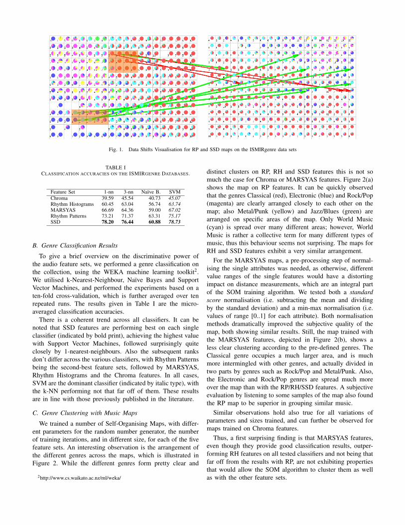
Fig. 1. Data Shifts Visualisation for RP and SSD maps on the ISMIRgenre data sets

TABLE ICLASSIFICATION ACCURACIES ON THE ISMIRGENRE DATABASES.

Feature Set 1-nn 3-nn Naı̈ve B. SVMChroma 39.59 45.54 40.73 45.07Rhythm Histograms 60.45 63.04 56.74 63.74MARSYAS 66.69 64.36 59.00 67.02Rhythm Patterns 73.21 71.37 63.31 75.17SSD 78.20 76.44 60.88 78.73

B. Genre Classification Results

To give a brief overview on the discriminative power ofthe audio feature sets, we performed a genre classification onthe collection, using the WEKA machine learning toolkit2.We utilised k-Nearest-Neighbour, Naı̈ve Bayes and SupportVector Machines, and performed the experiments based on aten-fold cross-validation, which is further averaged over tenrepeated runs. The results given in Table I are the micro-averaged classification accuracies.

There is a coherent trend across all classifiers. It can benoted that SSD features are performing best on each singleclassifier (indicated by bold print), achieving the highest valuewith Support Vector Machines, followed surprisingly quiteclosely by 1-nearest-neighbours. Also the subsequent ranksdon’t differ across the various classifiers, with Rhythm Patternsbeing the second-best feature sets, followed by MARSYAS,Rhythm Histograms and the Chroma features. In all cases,SVM are the dominant classifier (indicated by italic type), withthe k-NN performing not that far off of them. These resultsare in line with those previously published in the literature.

C. Genre Clustering with Music Maps

We trained a number of Self-Organising Maps, with differ-ent parameters for the random number generator, the numberof training iterations, and in different size, for each of the fivefeature sets. An interesting observation is the arrangement ofthe different genres across the maps, which is illustrated inFigure 2. While the different genres form pretty clear and

2http://www.cs.waikato.ac.nz/ml/weka/

distinct clusters on RP, RH and SSD features this is not somuch the case for Chroma or MARSYAS features. Figure 2(a)shows the map on RP features. It can be quickly observedthat the genres Classical (red), Electronic (blue) and Rock/Pop(magenta) are clearly arranged closely to each other on themap; also Metal/Punk (yellow) and Jazz/Blues (green) arearranged on specific areas of the map. Only World Music(cyan) is spread over many different areas; however, WorldMusic is rather a collective term for many different types ofmusic, thus this behaviour seems not surprising. The maps forRH and SSD features exhibit a very similar arrangement.

For the MARSYAS maps, a pre-processing step of normal-ising the single attributes was needed, as otherwise, differentvalue ranges of the single features would have a distortingimpact on distance measurements, which are an integral partof the SOM training algorithm. We tested both a standardscore normalisation (i.e. subtracting the mean and dividingby the standard deviation) and a min-max normalisation (i.e.values of range [0..1] for each attribute). Both normalisationmethods dramatically improved the subjective quality of themap, both showing similar results. Still, the map trained withthe MARSYAS features, depicted in Figure 2(b), shows aless clear clustering according to the pre-defined genres. TheClassical genre occupies a much larger area, and is muchmore intermingled with other genres, and actually divided intwo parts by genres such as Rock/Pop and Metal/Punk. Also,the Electronic and Rock/Pop genres are spread much moreover the map than with the RP/RH/SSD features. A subjectiveevaluation by listening to some samples of the map also foundthe RP map to be superior in grouping similar music.

Similar observations hold also true for all variations ofparameters and sizes trained, and can further be observed formaps trained on Chroma features.

Thus, a first surprising finding is that MARSYAS features,even though they provide good classification results, outper-forming RH features on all tested classifiers and not being thatfar off from the results with RP, are not exhibiting propertiesthat would allow the SOM algorithm to cluster them as wellas with the other feature sets.

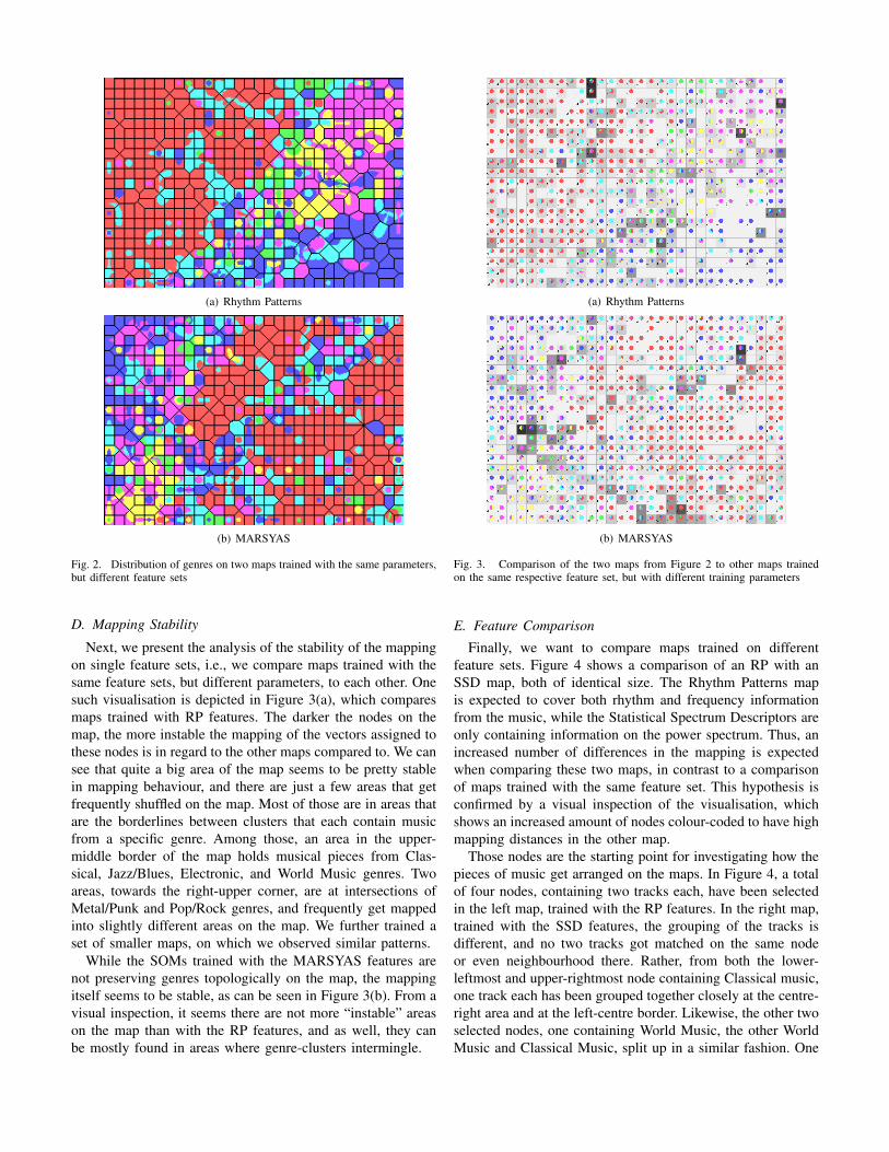
(a) Rhythm Patterns

(b) MARSYAS

Fig. 2. Distribution of genres on two maps trained with the same parameters,but different feature sets

D. Mapping Stability

Next, we present the analysis of the stability of the mappingon single feature sets, i.e., we compare maps trained with thesame feature sets, but different parameters, to each other. Onesuch visualisation is depicted in Figure 3(a), which comparesmaps trained with RP features. The darker the nodes on themap, the more instable the mapping of the vectors assigned tothese nodes is in regard to the other maps compared to. We cansee that quite a big area of the map seems to be pretty stablein mapping behaviour, and there are just a few areas that getfrequently shuffled on the map. Most of those are in areas thatare the borderlines between clusters that each contain musicfrom a specific genre. Among those, an area in the upper-middle border of the map holds musical pieces from Clas-sical, Jazz/Blues, Electronic, and World Music genres. Twoareas, towards the right-upper corner, are at intersections ofMetal/Punk and Pop/Rock genres, and frequently get mappedinto slightly different areas on the map. We further trained aset of smaller maps, on which we observed similar patterns.

While the SOMs trained with the MARSYAS features arenot preserving genres topologically on the map, the mappingitself seems to be stable, as can be seen in Figure 3(b). From avisual inspection, it seems there are not more “instable” areason the map than with the RP features, and as well, they canbe mostly found in areas where genre-clusters intermingle.

(a) Rhythm Patterns

(b) MARSYAS

Fig. 3. Comparison of the two maps from Figure 2 to other maps trainedon the same respective feature set, but with different training parameters

E. Feature Comparison

Finally, we want to compare maps trained on differentfeature sets. Figure 4 shows a comparison of an RP with anSSD map, both of identical size. The Rhythm Patterns mapis expected to cover both rhythm and frequency informationfrom the music, while the Statistical Spectrum Descriptors areonly containing information on the power spectrum. Thus, anincreased number of differences in the mapping is expectedwhen comparing these two maps, in contrast to a comparisonof maps trained with the same feature set. This hypothesis isconfirmed by a visual inspection of the visualisation, whichshows an increased amount of nodes colour-coded to have highmapping distances in the other map.

Those nodes are the starting point for investigating how thepieces of music get arranged on the maps. In Figure 4, a totalof four nodes, containing two tracks each, have been selectedin the left map, trained with the RP features. In the right map,trained with the SSD features, the grouping of the tracks isdifferent, and no two tracks got matched on the same nodeor even neighbourhood there. Rather, from both the lower-leftmost and upper-rightmost node containing Classical music,one track each has been grouped together closely at the centre-right area and at the left-centre border. Likewise, the other twoselected nodes, one containing World Music, the other WorldMusic and Classical Music, split up in a similar fashion. One

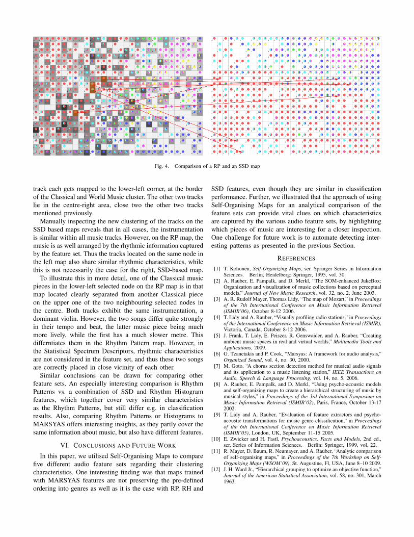
Fig. 4. Comparison of a RP and an SSD map

track each gets mapped to the lower-left corner, at the borderof the Classical and World Music cluster. The other two trackslie in the centre-right area, close two the other two tracksmentioned previously.

Manually inspecting the new clustering of the tracks on theSSD based maps reveals that in all cases, the instrumentationis similar within all music tracks. However, on the RP map, themusic is as well arranged by the rhythmic information capturedby the feature set. Thus the tracks located on the same node inthe left map also share similar rhythmic characteristics, whilethis is not necessarily the case for the right, SSD-based map.

To illustrate this in more detail, one of the Classical musicpieces in the lower-left selected node on the RP map is in thatmap located clearly separated from another Classical pieceon the upper one of the two neighbouring selected nodes inthe centre. Both tracks exhibit the same instrumentation, adominant violin. However, the two songs differ quite stronglyin their tempo and beat, the latter music piece being muchmore lively, while the first has a much slower metre. Thisdifferntiates them in the Rhythm Pattern map. However, inthe Statistical Spectrum Descriptors, rhythmic characteristicsare not considered in the feature set, and thus these two songsare correctly placed in close vicinity of each other.

Similar conclusions can be drawn for comparing otherfeature sets. An especially interesting comparison is RhythmPatterns vs. a combination of SSD and Rhythm Histogramfeatures, which together cover very similar characteristicsas the Rhythm Patterns, but still differ e.g. in classificationresults. Also, comparing Rhythm Patterns or Histograms toMARSYAS offers interesting insights, as they partly cover thesame information about music, but also have different features.

VI. CONCLUSIONS AND FUTURE WORK

In this paper, we utilised Self-Organising Maps to comparefive different audio feature sets regarding their clusteringcharacteristics. One interesting finding was that maps trainedwith MARSYAS features are not preserving the pre-definedordering into genres as well as it is the case with RP, RH and

SSD features, even though they are similar in classificationperformance. Further, we illustrated that the approach of usingSelf-Organising Maps for an analytical comparison of thefeature sets can provide vital clues on which characteristicsare captured by the various audio feature sets, by highlightingwhich pieces of music are interesting for a closer inspection.One challenge for future work is to automate detecting inter-esting patterns as presented in the previous Section.

REFERENCES

[1] T. Kohonen, Self-Organizing Maps, ser. Springer Series in InformationSciences. Berlin, Heidelberg: Springer, 1995, vol. 30.

[2] A. Rauber, E. Pampalk, and D. Merkl, “The SOM-enhanced JukeBox:Organization and visualization of music collections based on perceptualmodels,” Journal of New Music Research, vol. 32, no. 2, June 2003.

[3] A. R. Rudolf Mayer, Thomas Lidy, “The map of Mozart,” in Proceedingsof the 7th International Conference on Music Information Retrieval(ISMIR’06), October 8-12 2006.

[4] T. Lidy and A. Rauber, “Visually profiling radio stations,” in Proceedingsof the International Conference on Music Information Retrieval (ISMIR),Victoria, Canada, October 8-12 2006.

[5] J. Frank, T. Lidy, E. Peiszer, R. Genswaider, and A. Rauber, “Creatingambient music spaces in real and virtual worlds,” Multimedia Tools andApplications, 2009.

[6] G. Tzanetakis and P. Cook, “Marsyas: A framework for audio analysis,”Organized Sound, vol. 4, no. 30, 2000.

[7] M. Goto, “A chorus section detection method for musical audio signalsand its application to a music listening station,” IEEE Transactions onAudio, Speech & Language Processing, vol. 14, no. 5, 2006.

[8] A. Rauber, E. Pampalk, and D. Merkl, “Using psycho-acoustic modelsand self-organizing maps to create a hierarchical structuring of music bymusical styles,” in Proceedings of the 3rd International Symposium onMusic Information Retrieval (ISMIR’02), Paris, France, October 13-172002.

[9] T. Lidy and A. Rauber, “Evaluation of feature extractors and psycho-acoustic transformations for music genre classification,” in Proceedingsof the 6th International Conference on Music Information Retrieval(ISMIR’05), London, UK, September 11-15 2005.

[10] E. Zwicker and H. Fastl, Psychoacoustics, Facts and Models, 2nd ed.,ser. Series of Information Sciences. Berlin: Springer, 1999, vol. 22.

[11] R. Mayer, D. Baum, R. Neumayer, and A. Rauber, “Analytic comparisonof self-organising maps,” in Proceedings of the 7th Workshop on Self-Organizing Maps (WSOM’09), St. Augustine, Fl, USA, June 8–10 2009.

[12] J. H. Ward Jr., “Hierarchical grouping to optimize an objective function,”Journal of the American Statistical Association, vol. 58, no. 301, March1963.