Analyst Optimism Loan Announcement and Firm Performance - Chang 2010

8/3/2019 Analyst Optimism Loan Announcement and Firm Performance - Chang 2010

http://slidepdf.com/reader/full/analyst-optimism-loan-announcement-and-firm-performance-chang-2010 1/33

Analysts’ Overoptimism, Bank Loan Announcement, and the

Borrowing Firms’ Long Run Performance

Shao Chi Changa

Ya Shin Chenga

Ming Tse Tsaia

a Department of Business Administration, National Cheng Kung University, Tainan Taiwan

Abstract

In this study, we test analysts’ forecasts for firms announcing bank loans, and the

relationship between these forecasts and the long-run performance of the firms. Banks

have greater access and resources to get more inside information and do monitoring of

the borrowing firms, actions which are costly for common outside investors, and thus a

bank loan agreement conveys the positive perceptions of the lender bank to other

participants in capital market. Analysts have been shown to be over-optimistic with

regard to the equity issuing company, and thus we attempt to test whether they are also

overoptimistic with regard to firms that receive bank loans. The empirical results in our

study show that analysts are over-optimistic about firms that announce bank loans, andthat this might be an explanation for the firms’ long-run underperformance.

Key words: bank loan announcement, analyst overoptimism, long run performance



1

I. Introduction

Bank loans are an important way for firms to raise capital. Billet, Flannery and

Garfinkel (2006) show that the bank loan financing firm have positive returns around

the bank loan announcement, but disappointing long-run stock performance in the

following three years. This return trend is similar to that seen for other announcements

of actions to raise capital. For example, after IPO announcement previous studies show

that on average the issuing firms have positive announcement stock returns over the

short run and relatively poor stock performance in the long run (Ritter 1991). Spiess

and Affleck-Graves (1995) also find the same phenomenon after SEO announcements.

With regard to companies making bank loan announcements, James (1987) and

Lummer and McConnell (1989) provide evidence to show such firms have significantly

positive abnormal returns in the short run, but poor long-run performance.

Ritter (1991) proposes that the difference between the short- and long-run stock

performance after IPO announcements may be due to investors early overoptimism.

However, in the long run, investors revise their expectations for the firms and the stock

price reverses to its true value. Rajan and Servas (1997) adopt the analysts’ forecasts as

a proxy of investors’ expectations to provide a more direct empirical test with regard to

investors’ overoptimism at IPO announcements. They find that analysts tend to be

overoptimistic about the earnings potential and long run growth prospects of recent

IPOs. Analysts’ overoptimism is a good proxy for that of investors, because the



2

opinions of the former tend to reflect or drive the expectations of the latter.

James (1987) examines whether banks delivers valuable information about their

borrowers to investors in the market. The empirical results show that the stock return

trend after bank loan announcements is similar to the stock return trend after IPO

announcements. However, to date there is still no direct evidence to support the

relationship between investors’ overoptimism and bank loan announcements with

regard to the inconsistence in short- and long-run performance of borrower firms. Rajan

and Servas (1997) use analysts’ forecasts to test the investors’ overoptimism with

regard to IPO firms. Consequently, in this study we adopt analysts’ forecasts to test

whether investors’ overoptimism could explain the short run positive and long run poor

stock performance.

Why are analysts over-optimistic with regard to firms announcing bank loans? There

are two hypotheses, as follows. First is the information asymmetry hypothesis (Lummer,

McConnell 1989; Diamond 1984). In this, banks are generally viewed as insiders that

have access to more private information about the borrowing firms. When banks

approve a loan contract, this decision signals the borrowers’ creditworthiness to other

participants in the capital market. Second is the monitoring hypothesis (Fama 1985;

Diamond 1991). In this view, compared to common investors, banks have more

resources and capabilities to supervise the company and prevent the occurrence of



3

moral hazard. In relation to this, banks can also enhance the value of borrowing firms

by efficient monitoring and reducing information asymmetry. James (1987) and

Lummer and McConnell (1989) provide empirical evidence to show that bank loan

agreements convey positive news to the stock market and result in positive

announcement excess returns. These benefits might thus explain the short run

overoptimism and long run reverse that accompanies the announcement of such

financing deals.

In this study, we attempt to test the relationship between bank loan announcements,

analysts’ forecasts, and the borrowers’ stock performance. We address three questions:

(1) Are analysts over-optimistic at bank loan announcements?

(2) Do analysts make systematic errors in forecasting the stock performance of firms

announcing bank loan financing?

(3) Is the long run stock performance of borrowing firms related to the analysts’

overoptimism?

The existing literature has found evidence of analysts’ overoptimism with regard to

the performance of IPO firms, but there is still no clear evidence either for or against

this for bank loan announcements. This study thus intends to fill this gap in the

literature. By observing analysts’ forecasts, we investigate whether investors’

overoptimism is one explanation for the short run positive stock performance and long



4

run underperformance of the firms announcing bank loan financing. There are four

sections in the rest of this paper, section II is the literature review and presents the

hypotheses, section III presents the data and methodology, section IV is the empirical

results, and section V is the conclusion.



5

II. Literatures and Hypotheses

In this paper we use analysts’ forecasts as the proxy of the investors’ expectations.

Michaely and Womack (1999) find that analyst specific dissemination tasks include

gathering new information, analyzing data, writing reports and provide

recommendations to buy-side investors. Givoly and Lakonishok (1979), and Fried

and Givoly (1982), Ackert and Athanassakos (2003) propose that analysts’ earnings

forecasts convey useful information to market participants. When the investors have

any doubts about the target firm, they tend to refer to the opinions of analysts.

Therefore, analysts’ forecasts play an important role to guide and even drive investors

to make their investment decisions.

Rajan and Servaes (1997) examine analysts’ forecasts following IPOs, and their

empirical results show that analysts are overoptimistic about both the earnings potential

and the long term growth prospects of IPO firms. They propose that this overoptimism

might result from a selection bias, because analysts have an incentive to follow firms

with better prospects. Dechow, Hutton, and Sloan (2000), and Chahine (2004), also

provide evidence to show that analysts are over-optimistic with regard to firms offering

equity, which stems from the fact that they are generally over-optimistic about raising

capital in equity market. In this study, we want to test whether analysts are also

over-optimistic with regard to bank loan announcement.

Eckbo (1986) shows that issuing debt does not significantly influence the stock price.



6

James (1987), Lummer and McConnell (1989), and James (2006) find positive stock

return responses to the announcement of new bank credit agreements which are larger

than the responses associated with announcement of private placements or public

straight debt offerings. There are two hypotheses to support the positive stock return of

borrowing firms after a bank loan announcement. First is the information asymmetry

hypothesis. Diamond (1984), Lummer and McConnell (1989), Best and Zhang (1993)

propose that the banks have more access to information which is not available to other

outside investors. Fama (1985) also claims that banks have intimate and continuing

business relationships with the borrowing firms, and thus have advantages over other

capital market participants with regard to evaluating them. Because banks have more

access to information, if they decide to lend money to a firm then the announcement

also conveys the banks’ positive perceptions to other investors in market. Second is the

monitoring hypothesis. Besanko and Kanatas (1993) develop a model to prove the

special role of bank lending, and show that banks provide monitoring for entrepreneurs.

Such monitoring enhances the entrepreneur effort and improves the odds of success for

any project. Thus, Besanko and Kanatas (1993) claim that if firms’ capital structure

includes more bank loans, then the firms’ stock price should be higher than the

equilibrium stock price because of these bank monitoring effects. Datta, Iskandar-Datta,

and Patel (1999) also propose the banks have lower monitoring costs with regard to



7

supervising borrowers, and that the cross-monitoring brings lower future debt costs.

These earlier studies suggest that the information asymmetry and monitoring

hypotheses both support the idea that bank loan announcements make outside investors

more confident about the borrowing firms’ future prospects. In addition, Zhaoyang and

Jian (2007) propose that analysts tend to overreact to good news, and thus because bank

loan announcements convey positive signals to investors, analysts might be

over-optimistic about such firms. Therefore we expect that analysts will be

over-optimistic following bank loan announcements.

Hypothesis 1: Analysts are over-optimistic when firms make bank loan announcements.

Dechow, Hutton and Sloan (2000) found sell-side analysts’ long-term forecasts are

systematically over-optimistic around equity offerings. Rajan and Servaes (1997) found

analysts systematically overestimate the earnings of IPO firms, with approximately a

five percent forecast error for the stock price. As the forecast window increases, so does

the forecast error. Analysts are not only over-optimistic with regard to equity offerings,

they are also more over-optimistic about the offering firms’ long-run rather than

short-run prospects. The arguments in these earlier studies motivate our second

hypothesis.

Hypothesis 2: Analysts make systematic errors in forecasting the performance of bank

loan financing firms.



8

Billet, Flannery, and Garfinkel (2006) find bank loan financing firms suffer negative

abnormal stock returns over the subsequent three years, and this long-run

underperformance is similar to that seen with other debt issuing or equity offering firms.

They also find that larger loans are followed by even worse stock performance.

The analysts’ forecasts and recommendations influence other participants in the

market. If analysts are over-optimistic with regard to the prospects of the bank loan

financing firms, we expect to see stock underperformance with such borrowers in the

long-run. Rajan and Servaes (1997) investigate the relationship between analysts’

overoptimism and the long-run stock performance of IPO firms. Their empirical results

show that such firms have worse stock performance when analysts are more optimistic

about their long-run growth prospects. Thus, we also expect that more analysts’

overoptimism is associated with worse long-run stock performance for firms

announcing bank loan financing.

Hypothesis 3: The long-run performance of firms announcing bank loans is negatively

related to analysts’ overoptimism.



9

III. Methodology and Data

Data

We collect the bank loan announcements of U.S. firms from the Factiva database by

searching for news from 1996 to 2003. The bank loan financing firms in our sample are

required to be listed on New York Stock Exchange (NYSE), National Association of

Securities Dealers Automated Quotations (NASDAQ), or American Stock Exchange

(AMEX). Because we need the analyst data, the analyst following information for the

bank loan financing firms must be available in the Institutional Brokers Estimate

System (IBES). Table 1 is the distribution of bank loan announcements from 1997 to

2003. In this period, 1,486 bank loan announcements were made, and there are 1,366

related analysts’ forecasts in IBES. Panel A shows the sample distribution for each year,

while Panel B shows the industry of the bank loan announcing firms, with the majority

being manufacturing companies.

------------------------------

Insert Table 1

------------------------------

Analyst Forecast Error and Overoptimism

We use the forecast error to test whether the analysts make systematic errors in

forecasting the bank loan financing firms’ performance. Forecast errors are calculated

as in this equation:



10

Forecast Earningsof Timetheat PriceStock

Forecast Earning- Earnings Actual Error Forecast Earnings =

Forecasts are available on a monthly basis and made for periods of up to two fiscal

years in the future. In order to test whether analysts’ forecasts become more accurate

over time, we calculate the difference between those made within one year after the

bank loan announcement, and those made from one to two years after the bank loan

announcement. For more evidence, we collect industry- (two-digit SIC code) and

size-matched firms from CRSP to adjust the forecast error to test whether the analysts

are more optimistic with regard the bank loan financing firms.

In addition to earnings forecast, analysts also make long-term earnings projections.

Rajan and Servaes (1997) indicate that the long-term earnings forecasts should be

thought of as a measure of the relative optimism of analysts. We present the long-term

growth forecasts from the bank loan announcement to two years later. The

industry-adjusted long-term growths forecasts are computed by subtracting the average

of all firms with the same two-digit SIC code.

Long-term Performance

Following Billet, Flannery, and Garfinkel (2006), we adopt the stock buy-and-hold

return and return of calendar time portfolio to measure the long-term performance of

the bank loan financing firms. In addition, we adjust the buy-and-hold return to the

following three benchmarks to reduce the bias: industry- and size-matched firm, CRSP



11

NYSE/AMEX/NASDAQ value weighted index, and CRSP NYSE/AMEX/NASDAQ

equal weighted index. The buy-and-hold abnormal returns (BHAR) for stock i from

time a to b is defined as:

b a,control,b a,i,b a,i,BHR -BHR BHAR =

Where BHRi,a,b is the buy-and-hold returns of the sample firm and BHRcontrol,a,b is the

buy-and-hold returns of the control benchmarks. We adopt the model in Rajan and

Servaes (1997) to measure the long run performance of bank loan announcements. We

divide our sample firms into quartiles according to their industry-adjusted long-term

growth forecasts and compare the benchmark adjusted long-term stock returns for the

bank loan borrowers in the different quartiles. We employ the first long-term earnings

growth made in the year after the bank loan announcement and exclude returns

computed over the first 252 trading days from our analysis, because not all growth

forecasts are available during this period. The industry-adjusted long-term growth

forecasts are computed by subtracting the average long-term growth forecast for firms

in the same industry from IBES.

We use the regression model to test the relationship between the analysts forecasts

and the long-run performance of bank loan financing firms. The dependent variable is

the buy-and-hold returns (BHAR), and the independent variable is the industry-adjusted

long-term growth forecast (LF) made by analysts. Additionally, we have several control



12

variables in this regression. The loan characteristic variables are as follows.

Relative loan size (RLS) is computed as the logarithm of the amount of a firm’s bank

loan divided by its market value. Relative loan size is statistically significant in Billet,

Flannery and Garfinkel’s (2006) research; they found larger relative loan sizes are

associated with worse ex-post peer-adjusted returns. Moreover, poor ex-ante performers

tend to take on relatively larger loans, on which the lender chargers a higher rate spread.

Consequently, we include this variable because relative loan size can significantly

affect borrowing firms’ long-term performance.

Frequency (FRE) is a dummy variable. If the news indicates that the agreement is new,

we classify it as a new loan, and the dummy variable value is zero. If the news indicates

that the agreement is a revision, extension, or replacement of existing credit agreements,

we classify it as a revised loan, and the dummy variable value is one. Lummer and

McConnell (1989) found only favorable loan revisions have positive abnormal returns,

and this suggests that revised loans are more likely than new ones to be based on a

strong banking relationship.

Bank number (BN) is a dummy variable. If a firm borrows from only one bank, we

classify it as a single loan, and the dummy variable value is zero. However, if a firm’s

bank loan is credited by many banks, we classify it as a syndicated loan, and the

dummy variable value is one. Preece and Mullineaux (1996) find that a borrower’s



13

announcement return is inversely related to the number of lenders in the loan syndicate.

This is because loans involving a large syndicate are more likely to suffer from the

hold-out problem and are more difficult to renegotiate if the borrower is financially

distressed. Therefore we include this variable to test whether single or syndicated loans

may affect future returns.

The firm characteristic variables are as follows:

Firm size (SIZE) is computed as the logarithm of the market value of equity. Billet,

Flannery and Garfinkel (2006) include firm size as one of their control variables.

Equity book-to-market ratio (BM) is computed as log of equity book value divided

by market value. Billet, Flannery and Garfinkel (2006) include equity’s book-to-market

ratio as one of their control variables. We construct our regression as follows:

i i 6 i 5 i 4 i 3 i 2 i i i ε BN β FRE β RLS β BM β SIZE β LF β α BHAR +++++++=

Mitchell and Stafford (2000) propose that each sample firm’s BHAR tends to be

correlated with other BHARs, and thus the significance of this statistic might be

overstated. They suggest using a calendar time portfolio to control the calendar time

event-clustering problem, and thus in this study we adopt the Fama and French (1993)

three-factor model to measure long-term abnormal stock returns.

t t t ft mt ft pt HMLSMB R R R R ε β β β α +++−+=− hsm )(

Where pt R

is the equal-weighted or capitalization value-weighted average raw return



14

for a stock in calendar month t (where a sample stock is included if month t is within

the 36-month period following its bank loan announcement). ft R is the one month

T-bill return, mt R is the CRSP value-weighted market index return, t SMB is the return

on a portfolio of small stocks minus the return on a portfolio of large stocks, and

t HML is the return on a portfolio of stocks with high book to market ratio minus the

return on a portfolio of stocks with low book-to-market ratio.

We also estimate the abnormal stock returns with a fourth factor, t UMD , which is the

return on high momentum stocks minus the return on low momentum stocks. Because

Carhart (1997) shows the importance of momentum in expected return measures, we

refer to the following model as the Carhart four-factor model:

t t t t ft mt ft pt UMD HMLSMB R R R R ε β β β β α ++++−+=− uhsm )(

We use the intercept term,α , in the three-factor and four-factor models to measure the

average monthly abnormal returns for the calendar time portfolio.



15

IV. Empirical Results

In this study, we use forecast errors and long-term growth projections to measure

analysts’ overoptimism. Earnings forecast errors are reported in Table 2. Panel A shows

the analysts forecasts made within one year of the bank loan announcement. The error

as a percentage of stock price is -0.001 for forecasts made for a three-month window,

and this rises to -0.005 when the window increases to nine months. After controlling the

forecast error for the size- and industry- matched firms, the adjusted forecast errors in

the fourth column are still significant. The results support the proposal that analysts are

over-optimistic with regard to firms with bank loan financing. Panel B reports the

forecast errors made from one to two years after the bank loan announcement, and the

forecast error is still significant. The results thus show that the forecast accuracy does

not improve one year after the bank loan announcement, which means that analysts

continue to be over-optimistic about firms with bank loan financing.

------------------------------

Insert Table 2

------------------------------

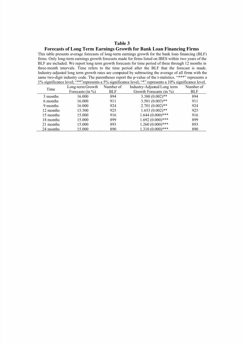
Analysts make long-term earnings growth projections to forecast firms’ growth

potential. Table 3 reports a detailed analysis of the long-term earnings growth forecasts

over a two-year period following the bank loan announcements. We only focus on the

growth forecasts for the last month of each quarter. Following Rajan and Servaes

(1997), we use the five-year horizon long-term forecast to measure the analysts’



16

accuracy. In Table 3, we find that the long-term growth forecasts within one year of a

bank loan announcement are about 16%. After more than one year after the bank loan

announcement, the growth forecasts decrease to 15%. In addition, we find that forecasts

for bank loan financing firms are 3.38% higher than for size and industry-matched

firms in the three- to six-month period after the bank loan announcement. After one

year, the growth expectations fall to about 1.65%, and then to only 1.31% two years

after the announcement. The results demonstrate that the analysts do indeed have more

optimistic expectations for bank loan financing firms. However, the shrinking

difference in long-term growth forecasts with regard to bank loan financing firms and

industrial average shows that analysts adjust their expectations over time.

------------------------------Insert Table 3

------------------------------

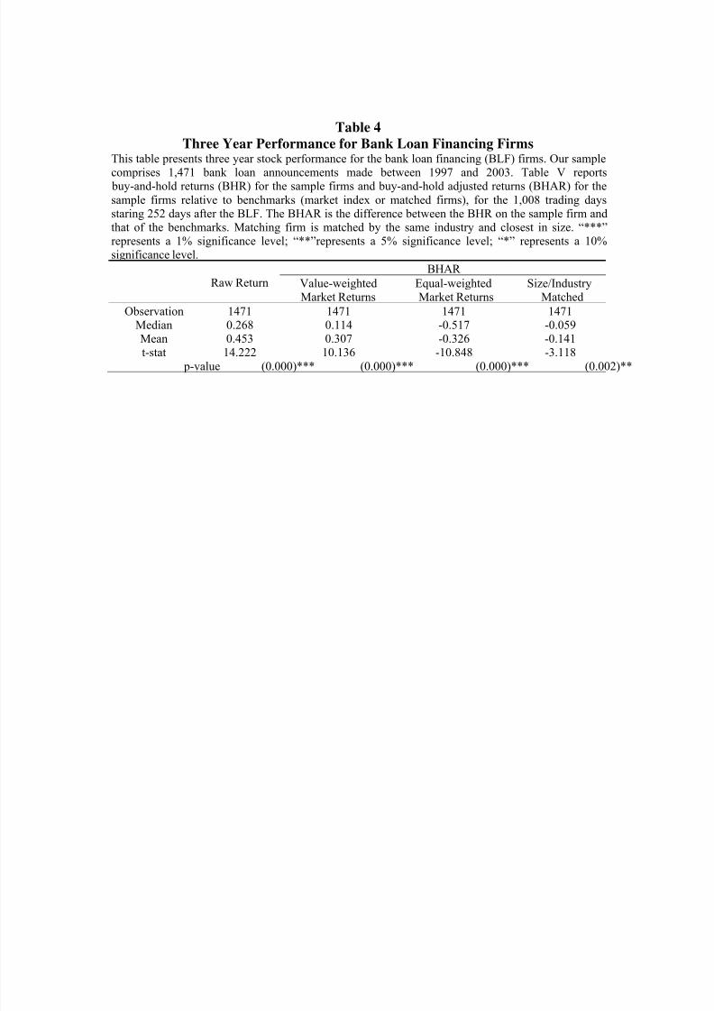
Table 4 shows descriptive statistics of the three-year buy-and-hold returns of the

bank loan financing firms. In addition to raw returns, we also try to control for the

value-weighted market returns, equal-weighted market returns, and size- and

industry-matched firms. After controlling for the equal-weighted market returns or size-

and industry-matched firms, we find that on average the bank loan financing firms

underperform in the long run.

------------------------------

Insert Table 4

------------------------------



17

We adopt the Fama French (1993) three-factor model and Carhart’s (1997)

four-factor model to test the long run performance of the bank loan financing firms. In

these two models, the intercept means the abnormal returns of the calendar time

portfolio. In Table 5, we can observe the significantly negative abnormal returns in

these models, which mean that on average the bank loan financing firms have poor

performance in the long run. We get the similar results using either value-weighted or

equal-weighted calendar-time portfolios.

------------------------------

Insert Table 5

------------------------------

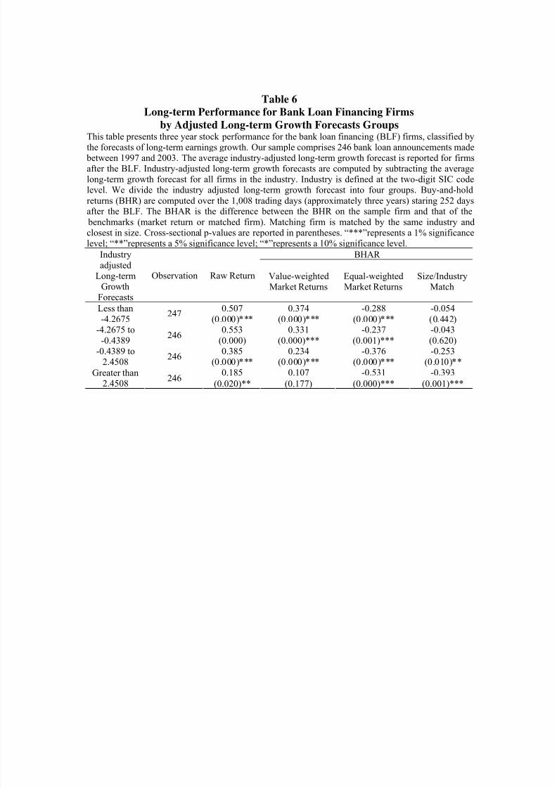
The results thus show that analysts have over-optimistic expectations for bank loan

financing firms, and that consequently the firms underperform in the long run. We try to

examine the relationship between analysts’ forecasts and the bank loan financing firms’

long-run performance. We use the forecasted industry adjusted growth quartiles model

that appears in Rajan and Servaes (1997). In Table 6, we use the quartiles as

benchmarks to divide the industry-adjusted long-term growth forecast into four groups.

Higher industry-adjusted long-term growth means analysts are more optimistic with

regard to the firms’ growth potential and future prospects. When the analysts make

more optimistic growth forecasts, the three-year buy-and-hold returns are lower. The

results in Table 6 show an inverse relationship between the analysts’ forecasts and the

long-run stock performance of the bank loan financing firms. The inverse relationship



18

provides evidence to support the notion that analysts are over-optimistic with regard to

the bank loan financing firms.

------------------------------

Insert Table 6

------------------------------

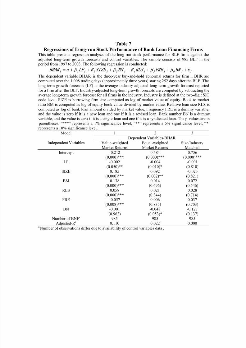
We also use regression to test the effect of analysts’ optimism on the borrowing firms.

We use the three years buy-and-hold returns as the dependent variable. The

buy-and-hold return is calculated from 256 to 1,008 trading days after the bank loan

announcement. The independent variable is the adjusted long-term growth forecast (LF)

made within 256 trading days after bank loan announcement. Additionally, there are

still other control variables to control effects from other possible factors. Table 7 shows

the regression results. In Models 1 and 2, the coefficients of the analysts’ long-term

forecast are negatively significant, even when other factors are controlled for. However,

Model 3 does not provide effective evidence of this, and its explanatory power is

weaker.

------------------------------

Insert Table 7

------------------------------

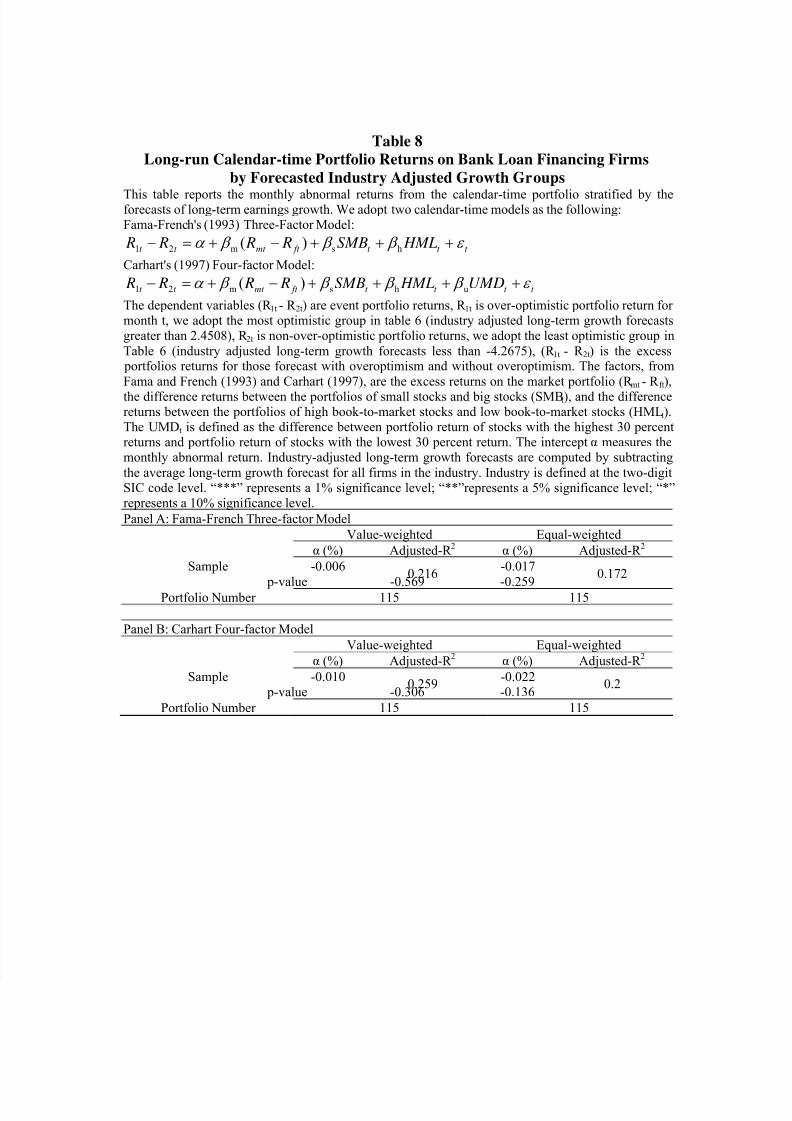
In addition to the regression model, we adopt calendar-time portfolios to examine the

relationship between analysts’ overoptimism and the long-term buy-and-hold returns

after bank loan announcements. In Table 8, we show the results of the Fama-French

(1993) three-factor and Carhart (1997) four-factor models. ( R1 - R2) is the excess



19

portfolios returns of those forecast with and without overoptimism. R1 is the

over-optimistic portfolio return for month t , we adopt the most optimistic group in

Table 6 (industry adjusted long-term growth forecasts greater than 2.4508). R 2 is

non-over-optimistic portfolio returns; we adopt the least optimistic group in Table 6

(industry adjusted long-term growth forecasts less than 4.2675). If α is negative, it

means that analysts’ overoptimism may lead to negative long-term abnormal returns. In

panels A and B of Table 8, the results of interceptα in value-weighted and

equal-weighted cases are both negative. This means that analysts’ overoptimism has an

inverse relation with bank loan financing firms’ long-term performance. This result is

also consistent with our expectation, and shows that higher analysts’ forecasts may lead

to worse long-term stock returns for bank loan financing firms.

------------------------------

Insert Table 8

------------------------------



20

V Conclusions

This study investigates whether or not analysts’ overoptimism can explain the negative

long-term performance of bank loan financing firms. We use earnings forecast errors

and long-term earning growth projections to examine analysts’ overoptimism.

Buy-and-hold abnormal returns and calendar-time portfolios are used to examine the

bank loan financing firms’ long run performance. Finally, we adopt the forecasted

industry adjusted growth quartiles model, regression model and calendar-time portfolio

regression model to examine the relationship between analysts’ overoptimism and the

long-term stock performance of bank loan financing firms.

This study has three major findings. First, analysts are systematically over-optimistic

with regard to bank loan financing firms, and they may adjust their forecasts over time.

Second, bank loan financing firms in our sample from 1997 to 2003 have negative

long-term stock performance. Equal-weighted BHAR returns, matched firm BHAR

returns, and the results of the Fama-French three-factor and Carhart four-factor

portfolio models all show that bank loan financing firms have negative long-term stock

returns. We thus conclude that bank loan financing firms may have negative long-term

abnormal returns. Third, firms perform poorly in the long run when analysts are more

optimistic about their long-run growth projections. The forecasted industry adjusted

growth quartiles model shows that the higher analysts’ long-term forecasts, the worse



21

the long-term performance. In the regression model, the results show an inverse

relationship between analysts’ long-term forecasts and the long-term stock performance

of bank loan financing firms. The results of the calendar-time portfolio model also

imply negative long-term performance for firms’ with over-optimistic forecasts.

Therefore, we can conclude that analyst overoptimism may be one explanation for bank

loan financing firms’ long run negative stock performance.

Analysts may issue favorable forecasts for some companies because they have a

relation with these firms, and want to bring in future investment banking business. So

analysts tend to give more coverage to these companies and provide over-optimistic

forecasts. Furthermore, Das et al. (2006) suggest that the new issue underperformance

puzzle exists among those firms which receive insufficient coverage. Therefore bank

loan financing firms’ negative long-term abnormal returns may result from the analysts’

selective coverage, and thus further studies can examine whether analysts have

relationships with the bank loan financing firms, and distinguish the purpose of their

forecast, to see whether they have any ulterior motive or not. By clarifying the

relationships with bank loan financing firms, we can better understand whether

analysts’ overoptimism is one explanation for bank loan financing firms’ long-term

negative returns.



References

Ackert, Lucy F., and George Athanassakos, 2003, A simultaneous equations analysis

of analysts' forecast bias, analyst following, and institutional ownership,

Journal of Business Finance & Accounting 30, 1017-1041.

Besanko, D., David Besanko, G. Kanatas, and George Kanatas, 1993, Credit market

equilibrium with bank monitoring and moral hazard, Review of Financial

Studies 6.

Best, Ronald, and Hang Zhang, 1993, Alternative information sources and the

information content of bank loans, Journal of Finance 48, 1507-1522.

Billet, Matthew T., Mark J. Flannery, and Jon A. Garfinkel, 2006, Are bank loans

special? Evidence on the post-announcement performance of bank borrowers,

Journal of Financial & Quantitative Analysis 41, 733-751.

Carhart, Mark M., 1997, On persistence in mutual fund performance, Journal of

Finance 52, 57-82.

Chahine, Salim, 2004, Long-run abnormal return after IPOs and optimistic analysts'

forecasts, International Review of Financial Analysis 13, 83.

Das, Somnath, G. U. O. Re-Jin, and Zhang Huai, 2006, Analysts' selective coverage

and subsequent performance of newly public firms, Journal of Finance 61,

1159-1185.

Datta, Sudip, Maik Iskandar-Datta, and Ajay Patel, 1999, Bank monitoring and the

pricing of corporate public debt, Journal of Financial Economics 51, 435-449.

Dechow, Patricia M., Amy P. Hutton, and Richard G. Sloan, 2000, The relation

between analysts' forecasts of long-term earnings growth and stock price

performance following equity offerings, Contemporary Accounting Research

17, 1-32.

Diamond, Douglas W., 1984, Financial intermediation and delegated monitoring,



Review of Economic Studies 51, 393.

Diamond, Douglas W., 1991, Monitoring and reputation: The choice between bank

loans and directly placed debt, Journal of Political Economy 99, 689.

Eckbo, B. Espen, 1986, Valuation effects of corporate debt offerings, Journal of

Financial Economics 15, 119-151.

Fama, Eugene F., 1985, What’s different about banks?, Journal of Monetary

Economics 15, 29-39.

Fama, Eugene F., and Kenneth R. French, 1993, Common risk factors in the returns

on stocks and bonds, Journal of Financial Economics 33, 3-56.

Fried, Dov, and Dan Givoly, 1982, Financial analysts' forecasts of earnings, Journal

of Accounting & Economics 4, 85-107.

Givoly, Dan, and Josef Lakonishok, 1979, The information content of financial

analysts' forecasts of earnings, Journal of Accounting & Economics 1,

165-185.

James, Christopher, 1987, Some evidence on the uniqueness of bank loans, Journal of

Financial Economics 19, 217-235.

James, Christopher, and Jason Karceski, 2006, Strength of analyst coverage following

IPOs, Journal of Financial Economics 82, 1-34.

Lummer, Scott L., and John J. McConnell, 1989, Further evidence on the bank

lending process and the capital-market response to bank loan agreements,

Journal of Financial Economics 25, 99-122.

Michaely, R., Roni Michaely, K. L. Womack, and Kent L. Womack, 1999, Conflict of

interest and the credibility of underwriter analyst recommendations, Review of

Financial Studies 12.

Mitchell, Mark L., and Erik Stafford, 2000, Managerial decisions and long-term stock

price performance, Journal of Business 73, 287.



Preece, Dianna, and Donald J. Mullineaux, 1996, Monitoring, loan renegotiability,

and firm value: The role of lending syndicates, Journal of Banking & Finance

20, 577-593.

Rajan, Raghuram, and Henri Servaes, 1997, Analyst following of initial public

offerings, Journal of Finance 52, 507-529.

Ritter, Jay R., 1991, The long-run performance of initial public offerings, Journal of

Finance 46, 3-27.

Spiess, D. Katherine, and John Affleck-Graves, 1995, Underperformance in long-run

stock returns following seasoned equity offerings, Journal of Financial

Economics 38, 243-267.

Zhaoyang, Gu, and Xue Jian, 2007, Do analysts overreact to extreme good news in

earnings?, Review of Quantitative Finance & Accounting 29, 415-431.



Table 1

Distribution of Bank Loan Financing FirmsThis table summarizes the sample distribution of bank loan financing firms listed on the New York

Stock Exchange (NYSE), the American Stock Exchange (AMEX), or the NASDAQ exchange from1997 to 2003. The sample is collected from the Factiva database. 1,486 firms meet the samplerestrictions. Number on Institutional Brokers Estimate System (IBES) refers to the number of bank loan financing (BLF) firms that listed on the IBES database within two years of the bank loan financing(BLF). The two-digit SIC code is obtained from Compustat.

Panel A: Distribution of Sample Over Time

Offering Year Observations % Available in IBES %

1997 157 10.49 145 10.611998 240 16.04 212 15.521999 298 19.92 270 19.772000 139 9.29 125 9.15

2001 154 10.29 142 10.402002 231 15.44 214 15.67

2003 267 17.85 258 18.89Total 1486 100 1366 100.00

Panel B: Distribution of Sample across Two-Digit SIC Codes

IndustryTwo-digit

SICObservations %

Available in

IBES%

Agriculture, Forest and Fishing 01~09 7 0.47 5 0.37Mining 10~14 82 5.52 81 5.93Construction 15~17 48 3.23 46 3.37Manufacturing 20~39 463 31.16 426 31.19Transportation and

Communications40~48 140 9.42 139 10.18

Wholesale Trade 50~51 80 5.38 68 4.98

Retail Trade 52~59 139 9.35 128 9.37

Finance, Insurance, and RealEstate

60~67 260 17.5 222 16.25

Services 70~89 263 17.7 247 18.08Public Administration 91~99 4 0.27 4 0.29Total 1486 100 1366 100



Table 2

Analyst Earnings Forecast Errors for Bank Loan Financing FirmsThis table presents average analyst earnings forecast errors for the bank loan financing firms. Our

sample comprises 1,486 companies between 1997 and 2003. Only earnings forecasts made for firmslisted on IBES within two years of the bank loan financing (BLF) are included. The forecast error is

computed as: (Actual earnings –Earnings forecast) / Stock price at the time of the earning forecasts.We report forecast errors for forecast windows of three through 12 months in three-month intervals.Window is the number of months between when the forecast is made and the fiscal year end for whichthe forecast is made. Matched firm adjusted forecast errors are computed by subtracting the forecasterror of the firm with the same SIC code closest in size to the BLF firm. The number of observations inthe matched firm adjusted sample is smaller, because no matched firms can be found for certainforecast windows. The parentheses report the p-value of the t-statistics. “***” represents a 1%significance level; “**”represents a 5% significance level; “*” represents a 10% significance level.

Panel A: Forecasts Made Within One Year of BLF

Window Forecast Error Number of BLFMatching Firm

Adjusted Forecast Error Number of BLF

3 -0.001 (0.000)*** 1052 -0.000 (0.043)** 8336 -0.003 (0.000)*** 1061 -0.001 (0.014)** 8379 -0.005 (0.000)*** 1035 -0.002 (0.000)*** 816

12 -0.002 (0.000)*** 626 -0.002 (0.003)*** 510

Panel B: Forecasts Made Between One and Two Years of BLF

Window Forecast Error Number of BLFMatching Firm

Adjusted Forecast Error Number of BLF

3 -0.001 (0.000)*** 1063 -0.000 (0.015)** 828

6 -0.003 (0.000)*** 1006 -0.002 (0.000)*** 7759 -0.005 (0.000)*** 972 -0.003 (0.000)*** 77112 -0.002 (0.000)*** 589 -0.003 (0.000)*** 484



Table 3

Forecasts of Long Term Earnings Growth for Bank Loan Financing FirmsThis table presents average forecasts of long-term earnings growth for the bank loan financing (BLF)

firms. Only long-term earnings growth forecasts made for firms listed on IBES within two years of theBLF are included. We report long term growth forecasts for time period of three through 12 months in

three-month intervals. Time refers to the time period after the BLF that the forecast is made.Industry-adjusted long term growth rates are computed by subtracting the average of all firms with thesame two-digit industry code. The parentheses report the p-value of the t-statistics. “***” represents a1% significance level; “**”represents a 5% significance level; “*” represents a 10% significance level.

TimeLong-term Growth

Forecasts (in %)

Number of

BLF

Industry-Adjusted Long term

Growth Forecasts (in %)

Number of

BLF

3 months 16.000 894 3.380 (0.002)** 8946 months 16.000 911 3.501 (0.003)** 9119 months 16.000 924 2.701 (0.002)** 92412 months 15.500 925 1.653 (0.002)** 92515 months 15.000 916 1.644 (0.000)*** 916

18 months 15.000 899 1.692 (0.000)*** 89921 months 15.000 893 1.260 (0.000)*** 893

24 months 15.000 890 1.310 (0.000)*** 890



Table 4

Three Year Performance for Bank Loan Financing FirmsThis table presents three year stock performance for the bank loan financing (BLF) firms. Our sample

comprises 1,471 bank loan announcements made between 1997 and 2003. Table V reports buy-and-hold returns (BHR) for the sample firms and buy-and-hold adjusted returns (BHAR) for the

sample firms relative to benchmarks (market index or matched firms), for the 1,008 trading daysstaring 252 days after the BLF. The BHAR is the difference between the BHR on the sample firm andthat of the benchmarks. Matching firm is matched by the same industry and closest in size. “***”represents a 1% significance level; “**”represents a 5% significance level; “*” represents a 10%significance level.

BHAR Raw Return Value-weighted

Market ReturnsEqual-weightedMarket Returns

Size/IndustryMatched

Observation 1471 1471 1471 1471Median 0.268 0.114 -0.517 -0.059Mean 0.453 0.307 -0.326 -0.141

t-stat 14.222 10.136 -10.848 -3.118 p-value (0.000)*** (0.000)*** (0.000)*** (0.002)**



Table 5

Long-run Returns Following Private Placements Calendar-Time PortfoliosThis table reports the unadjusted intercept from calendar-time portfolio regressions:

Fama-French's (1993) Three-Factor Model:t t t ft mt ft pt HMLSMB R R R R ε β β β α +++−+=− hsm )(

Carhart' s (1997) Four-factor Model:

t t t t ft mt ft pt UMD HMLSMB R R R R ε β β β β α ++++−+=− uhsm )(

The dependent variables (R pt - R ft) are event portfolio returns, R p, in excess of the treasury bill rate, R ft.

Each month, we form a portfolio of all sample firms that have BLF from 13th month to 48th month.The factors, from Fama and French (1993) and Carhart (1997), are the excess returns on the market portfolio (R pt - R ft), the difference in returns between the portfolios of small stocks and big stocks(SMBt), and the difference in returns between the portfolios of high book-to-market stocks and low book-to-market stocks (HMLt). The UMDt is defined as the difference between a portfolio return of stocks with the highest 30 percent returns and a portfolio return of stocks with the lowest 30 percentreturns. The intercept α measures the monthly abnormal returns, given the model. “***” represents a

1% significance level; “**”represents a 5% significance level; “*” represents a 10% significance level.Panel A: Fama-French Three-factor Model

Value-weighted Equal-weighted

α Adjusted-R 2 α Adjusted-R 2

Sample -0.007 -0.008 p-value (0.028)**

0.216(0.003)***

0.676

Portfolio Number 115 115

Panel B: Carhart Four-factor Model


α Adjusted-R 2 α Adjusted-R

2

Sample -0.006 -0.007 p-value (0.043)**

0.259(0.010)***

0.692




Table 6

Long-term Performance for Bank Loan Financing Firms

by Adjusted Long-term Growth Forecasts Groups

This table presents three year stock performance for the bank loan financing (BLF) firms, classified bythe forecasts of long-term earnings growth. Our sample comprises 246 bank loan announcements made between 1997 and 2003. The average industry-adjusted long-term growth forecast is reported for firmsafter the BLF. Industry-adjusted long-term growth forecasts are computed by subtracting the averagelong-term growth forecast for all firms in the industry. Industry is defined at the two-digit SIC codelevel. We divide the industry adjusted long-term growth forecast into four groups. Buy-and-hold

returns (BHR) are computed over the 1,008 trading days (approximately three years) staring 252 daysafter the BLF. The BHAR is the difference between the BHR on the sample firm and that of the

benchmarks (market return or matched firm). Matching firm is matched by the same industry andclosest in size. Cross-sectional p-values are reported in parentheses. “***”represents a 1% significancelevel; “**”represents a 5% significance level; “*”represents a 10% significance level.

BHAR Industryadjusted

Long-termGrowth

Forecasts

Observation Raw Return Value-weightedMarket Returns

Equal-weightedMarket Returns

Size/IndustryMatch

0.507 0.374 -0.288 -0.054Less than-4.2675

247(0.000)*** (0.000)*** (0.000)*** (0.442)

0.553 0.331 -0.237 -0.043-4.2675 to

-0.4389246

(0.000) (0.000)*** (0.001)*** (0.620)0.385 0.234 -0.376 -0.253-0.4389 to

2.4508246

(0.000)*** (0.000)*** (0.000)*** (0.010)**0.185 0.107 -0.531 -0.393Greater than

2.4508246

(0.020)** (0.177) (0.000)*** (0.001)***



Table 7

Regressions of Long-run Stock Performance of Bank Loan Financing FirmsThis table presents regression analyses of the long run stock performance for BLF firms against the

adjusted long-term growth forecasts and control variables. The sample consists of 985 BLF in the period from 1997 to 2003. The following regression is conducted:

i i 6 i 5 i 4 i 3 i 2 i i i ε BN β FRE β RLS β BM β SIZE β LF β α BHAR +++++++=

The dependent variable BHAR i is the three-year buy-and-hold abnormal returns for firm i. BHR arecomputed over the 1,008 trading days (approximately three years) staring 252 days after the BLF. Thelong-term growth forecasts (LF) is the average industry-adjusted long-term growth forecast reportedfor a firm after the BLF. Industry-adjusted long-term growth forecasts are computed by subtracting theaverage long-term growth forecast for all firms in the industry. Industry is defined at the two-digit SICcode level. SIZE is borrowing firm size computed as log of market value of equity. Book to market

ratio BM is computed as log of equity book value divided by market value. Relative loan size RLS iscomputed as log of bank loan amount divided by market value. Frequency FRE is a dummy variable,and the value is zero if it is a new loan and one if it is a revised loan. Bank number BN is a dummyvariable, and the value is zero if it is a single loan and one if it is a syndicated loan. The p-values are in

parentheses. “***” represents a 1% significance level; “**” represents a 5% significance level; “*”represents a 10% significance level.

Model 1 2 3

Dependent Variables-BHAR Independent Variables Value-weighted

Market ReturnsEqual-weightedMarket Returns

Size/IndustryMatched

Intercept -0.212 0.584 0.756(0.000)*** (0.000)*** (0.000)***

LF -0.002 -0.004 -0.001

(0.050)** (0.010)* (0.810)SIZE 0.185 0.092 -0.023

(0.000)*** (0.002)** (0.821)

BM 0.138 0.014 0.072(0.000)*** (0.696) (0.546)RLS 0.058 0.021 0.028

(0.000)*** (0.344) (0.714)FRE -0.057 0.006 0.037

(0.008)*** (0.835) (0.703)BN -0.001 -0.048 -0.127

(0.962) (0.053)* (0.137)985 985 985 Number of BNFa

Adjusted-R 2

0.110 0.022 0.000a Number of observations differ due to availability of control variables data .



Table 8

Long-run Calendar-time Portfolio Returns on Bank Loan Financing Firms

by Forecasted Industry Adjusted Growth Groups

This table reports the monthly abnormal returns from the calendar-time portfolio stratified by theforecasts of long-term earnings growth. We adopt two calendar-time models as the following:Fama-French's (1993) Three-Factor Model:

t t t ft mt t t HMLSMB R R R R ε β β β α +++−+=− hsm21 )(

Carhart's (1997) Four-factor Model:

t t t t ft mt t t UMD HMLSMB R R R R ε β β β β α ++++−+=− uhsm21 )(

The dependent variables (R 1t - R 2t) are event portfolio returns, R 1t is over-optimistic portfolio return for month t, we adopt the most optimistic group in table 6 (industry adjusted long-term growth forecastsgreater than 2.4508), R 2t is non-over-optimistic portfolio returns, we adopt the least optimistic group in

Table 6 (industry adjusted long-term growth forecasts less than -4.2675), (R 1t - R 2t) is the excess portfolios returns for those forecast with overoptimism and without overoptimism. The factors, from

Fama and French (1993) and Carhart (1997), are the excess returns on the market portfolio (R mt - R ft),

the difference returns between the portfolios of small stocks and big stocks (SMBt), and the differencereturns between the portfolios of high book-to-market stocks and low book-to-market stocks (HML t).The UMDt is defined as the difference between portfolio return of stocks with the highest 30 percentreturns and portfolio return of stocks with the lowest 30 percent return. The intercept α measures themonthly abnormal return. Industry-adjusted long-term growth forecasts are computed by subtracting

the average long-term growth forecast for all firms in the industry. Industry is defined at the two-digitSIC code level. “***” represents a 1% significance level; “**”represents a 5% significance level; “*”represents a 10% significance level.

Panel A: Fama-French Three-factor Model


α (%) Adjusted-R 2 α (%) Adjusted-R 2

Sample -0.006 -0.017

p-value -0.5690.216

-0.2590.172


Panel B: Carhart Four-factor Model


α (%) Adjusted-R 2 α (%) Adjusted-R

2

Sample -0.010 -0.022 p-value -0.306

0.259-0.136

0.2


Analyst Optimism Loan Announcement and Firm Performance - Chang 2010

Documents

Transcript of Analyst Optimism Loan Announcement and Firm Performance - Chang 2010