Analysis software for the preparation of the antenna

MIN LI / HAILONG LIANG Analysis software for the preparationof the antenna characteristics in the wireless system

1

FACULTYFACULTYFACULTYFACULTY OFOFOFOF ENGINEERINGENGINEERINGENGINEERINGENGINEERING ANDANDANDAND SUSTAINABLESUSTAINABLESUSTAINABLESUSTAINABLE DEVELOPMENTDEVELOPMENTDEVELOPMENTDEVELOPMENT

Analysis software for the preparationof the antenna characteristics in the wireless system

Min Li(880408-0748)

Hailong Liang(881231-4097)

September, 2012

BachelorBachelorBachelorBachelor’’’’ssss thesisthesisthesisthesis inininin electronicelectronicelectronicelectronic

BachelorBachelorBachelorBachelor’’’’ssss ProgramProgramProgramProgram inininin ElectronicsElectronicsElectronicsElectronics

Examiner:Examiner:Examiner:Examiner:NiklasNiklasNiklasNiklas RothpfefferRothpfefferRothpfefferRothpfeffer

Supervisor:Supervisor:Supervisor:Supervisor: JoseJoseJoseJose ChiloChiloChiloChilo


2

PrefacePrefacePrefacePreface

First and foremost, we would like to express my heartfelt gratitude to our supervisor,

Jose Chilo and examiner, Niklas Rothpfeffer, who give us considerable help to

complete this thesis. Second I would like to thank all of our college teachers who have

enlarged our knowledge and horizon during my studying. Third we would like to

thank our friends and classmates who help a lot..


3

AbstractAbstractAbstractAbstract

With the development of the wireless communication system, the antenna has been

widely used as an important tool in data transmission. However, there are many

characteristic parameters for antenna need to be calculated by complex calculation.

For example the mutual input impedance of dipole antenna, the Directivity coefficient

and the Gain coefficient. Therefore, it is quite practically hard to implement by hand,

especially for student who was studying on it. In order to solve this problem, this

thesis has establishes the calculation procedure for the complex parameters of antenna

by using MATLAB software.

KeyKeyKeyKey works:works:works:works:

MATLAB, GUI, SCIENTIFIC CALCULATOR, ANTENNA


4

TableTableTableTable ofofofof contentscontentscontentscontents

Abstract................................................................................................................... 3

Table of contents..................................................................................................... 4

1. Introduction......................................................................................................... 6

1.1 Background................................................................................................... 6

1.2 Aim of thesis..................................................................................................6

1.3 Delimitations................................................................................................. 7

2. Theory................................................................................................................. 8

2.1 Antenna..........................................................................................................8

2.1.1 The basics of the antenna dipole.............................................................. 8

2.1.2 Symmetric dipole..................................................................................... 9

2.1.3 Input impedance of symmetric dipole.................................................... 11

2.1.4 Radiation impedance of coupled symmetric dipole............................... 15

2.1.5 Directivity factor and gain coefficient of antenna.................................. 19

2.2. Matlab background.....................................................................................24

2.3 Matlab GUI introduce................................................................................. 25

3. Process and Result .............................................................................................27

3.1 The antenna parameter calculation software design....................................27

3.1.1 Flow chart of design a GUI interface..................................................... 27

3.2The specific process..................................................................................... 28

3.2.1 Generation of Main-dialog box.............................................................. 28

3.2.2 Generation of sub-dialog box................................................................. 29

4. Result.................................................................................................................35

4.1 Interface functional verification.................................................................. 35

4.3 Mutual radiation impedance function verification...................................... 37

4.4 The directional coefficient and the validation of the gain coefficient......... 38

4.5 Input resistance curve Plot.......................................................................... 39

4.6 Input reactance Curve Plot.............................................................................. 40

5. Discussion......................................................................................................... 41


5

6. Conclusion.........................................................................................................42

7. Reference:..........................................................................................................43

8. Appendix........................................................................................................... 45

8.1 Main dialogue code......................................................................................... 45

8.2 Mutual radiation impedance........................................................................ 46

8.3 The calculated directivity coefficient and gain coefficient ......................... 47

8.4 input resistance curve.................................................................................. 48

8.5 Draw input reactance curve......................................................................... 48


6

1.1.1.1. IntroductionIntroductionIntroductionIntroduction

1.11.11.11.1BackgroundBackgroundBackgroundBackground

When study the subject antenna there are many significant electrical parameter

calculations which are quite complicated. It is necessary to integrate the value of

complex functions. To complete the overall process calculation, it will waste a lot of

time. Teacher usually gives students some common numerical form for consulting. In

this way, students would make no account of the computational method of important

parameters. Since they only apply ready-made results, nevertheless, when they solve

the practical problems they don’t even know where to start. It is not good for training

research-based learning of students.

MATLAB has powerful scientific calculations and visible functions. It is simple and

easy to use. It is a basic tool and preferred platform which can help computers to

design, analysis and algorithmic research. GUI is used widely which is more

friendliness, intuitiveness, mobility. This article used MATLAB to design a GUI by

scientific calculation interface. Thus researchers can calculate the complex calculation

in an easy way of antenna parameter.

1.21.21.21.2AimAimAimAim ofofofof thesisthesisthesisthesis

The purpose of this thesis is to draw up the software for calculation of important

antenna parameters and software need to input parameter by students themselves. The

mainly work is to make a working software interface. First of all researchers need to

establish a main dialog box and make calculate parameters interface in the main

dialog box. Then click parameter buttons what researchers need to calculate. In this

way, researchers can enter the interface which shows the calculate parameters, input

relevant conditions and formulas to get parameter results. The difficult points of this

thesis are integral calculations and how to use the parameter and equation into the


7

programming.

Students can input parameters to calculate relevant complex antenna parameters

though the software. By calculating mutual radiation impedance, radiation impedance,

directivity and gain coefficient of an antenna and so on, students can expand the

understanding to the antenna’s characteristic . Meanwhile, by calculating many sets of

data, students also can strengthen the comprehending of the regularity which changes

with parameters.

1.31.31.31.3 DelimitationsDelimitationsDelimitationsDelimitations

This thesis is mainly used for education of students. This article is focus on

investigate the characteristic of dipole antenna’s calculation by using Matlab GUI

interfaces. The aim of this project is to establish a basic platform to research.


8

2222 TTTTheoryheoryheoryheory

2.12.12.12.1AntennaAntennaAntennaAntenna

2.1.12.1.12.1.12.1.1 TheTheTheThe basicsbasicsbasicsbasics ofofofof thethethethe antennaantennaantennaantenna dipoledipoledipoledipole

An antenna is a device that is used to transfer guided electromagnetic waves (signals)

to radiating waves in an unbounded medium, usually free space, and vice versa (i.e.,

in either the transmitting or receiving mode of operation). Antennas are

frequency-dependent devices. Each antenna is designed for a certain frequency band.

Beyond the operating band, the antenna rejects the signal. [1]

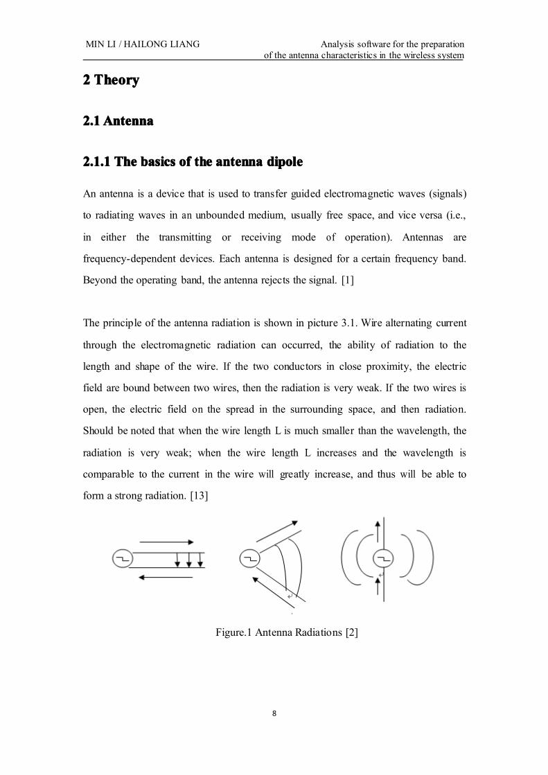
The principle of the antenna radiation is shown in picture 3.1. Wire alternating current

through the electromagnetic radiation can occurred, the ability of radiation to the

length and shape of the wire. If the two conductors in close proximity, the electric

field are bound between two wires, then the radiation is very weak. If the two wires is

open, the electric field on the spread in the surrounding space, and then radiation.

Should be noted that when the wire length L is much smaller than the wavelength, the

radiation is very weak; when the wire length L increases and the wavelength is

comparable to the current in the wire will greatly increase, and thus will be able to

form a strong radiation. [13]

Figure.1 Antenna Radiations [2]


9

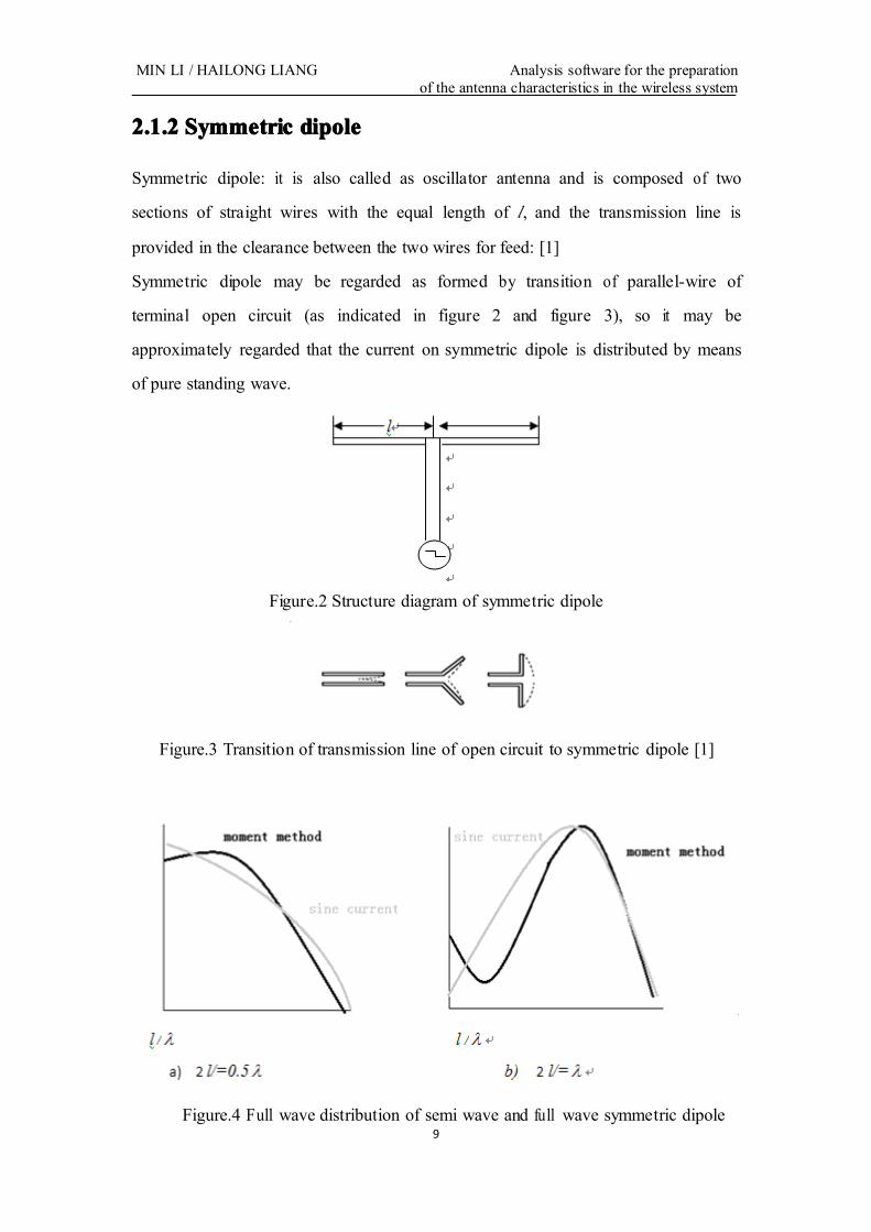
2.1.22.1.22.1.22.1.2 SSSSymmetricymmetricymmetricymmetric dipoledipoledipoledipole

Symmetric dipole: it is also called as oscillator antenna and is composed of two

sections of straight wires with the equal length of l, and the transmission line is

provided in the clearance between the two wires for feed: [1]

Symmetric dipole may be regarded as formed by transition of parallel-wire of

terminal open circuit (as indicated in figure 2 and figure 3), so it may be

approximately regarded that the current on symmetric dipole is distributed by means

of pure standing wave.

Figure.2 Structure diagram of symmetric dipole

Figure.3 Transition of transmission line of open circuit to symmetric dipole [1]

Figure.4 Full wave distribution of semi wave and full wave symmetric dipole


10

Analytic expression of current distribution is:

⎩⎨⎧

>−

<+=

0 )]('sin[0 )]('sin[

)(zzlIzzlI

zIM

M

ββ

(2.1)

IM: wave loop current amplitude on symmetric oscillator;

β ': phase constant of symmetric oscillator current，β '≈β.

Figure.5 Coordinate system of the symmetric dipole

Divide the symmetric dipole into infinite number of element lengths and each element

length may be regarded as a current element I (z)dz.

The known radiation field of current element is

r

rlI

rIljrEE β

θ θλ

ϕθ jrj-0 e sin 60jesin

2),,( −β π

=θηλ

== (2.2)

Select a current element on point z1 of left arm and point z2 of right arm on symmetric

dipole:

d)](sin[d)( 1111 zzlIzzI M += β (z1<0)

2222 d)](sin[d)( zzlIzzI M −= β (z2>0)

r1 = r－z1cosθ

r2 = r－z2cosθ (2.3)


11

Note: the observation point is far to the symmetric dipole, so it may be approximately

regarded that θ1 = θ2 = θ.

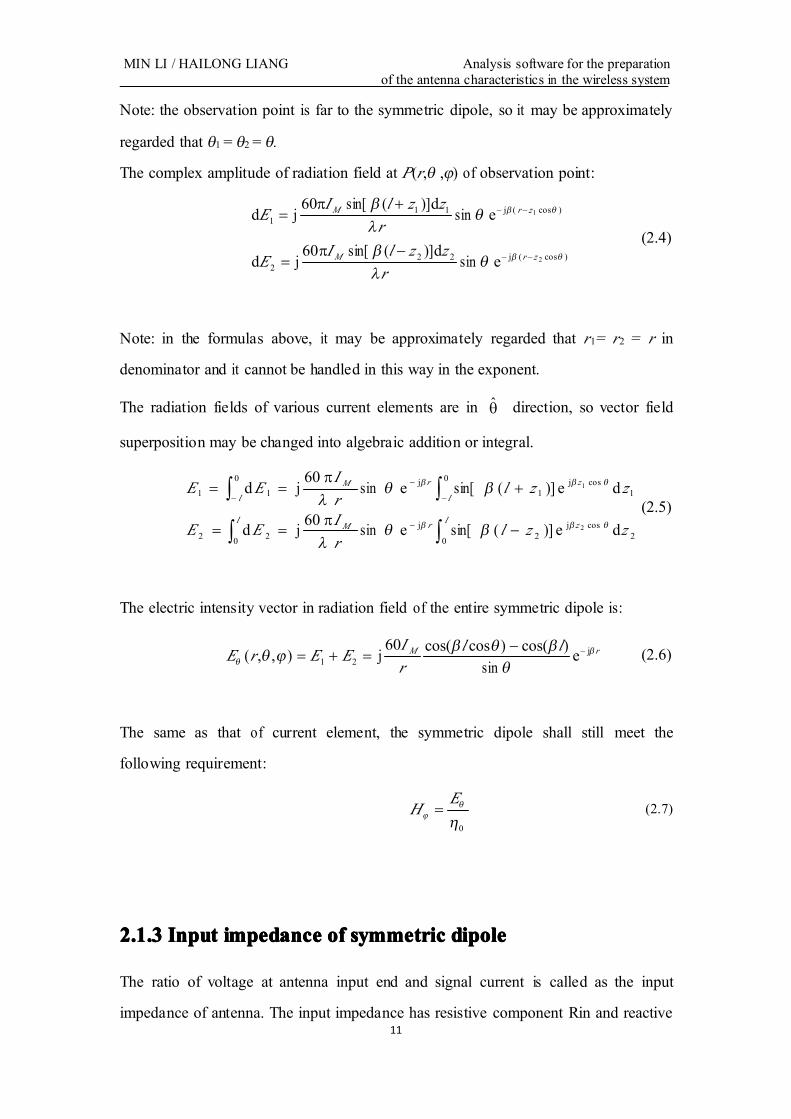
The complex amplitude of radiation field at P(r,θ ,ϕ) of observation point:

)cos (j222

)cos (j111

2

1

e sind)](sin[60

jd

e sind)](sin[60

jd

θβ

θβ

θλβ

θλβ

zrM

zrM

rzzlI

E

rzzlI

E

−−

−−

−π=

+π=

(2.4)

Note: in the formulas above, it may be approximately regarded that r1= r2 = r in

denominator and it cannot be handled in this way in the exponent.

The radiation fields of various current elements are in θ direction, so vector field

superposition may be changed into algebraic addition or integral.

∫∫

∫∫

−π

==

+π

==

−

−

−

−

l zrMl

l

zrMl

zzlrIEE

zzlrI

EE

0 2cosj

2j

0 22

0

1cosj

1j0

11

de)](sin[e sin

60jd

de)](sin[e sin

60jd

2

1

θββ

θββ

βθλ

βθλ (2.5)

The electric intensity vector in radiation field of the entire symmetric dipole is:

rM llrI

EErE βθ θ

βθβϕθ j21 e

sin)cos()coscos(60

j),,( −−=+= (2.6)

The same as that of current element, the symmetric dipole shall still meet the

following requirement:

0ηθ

ϕ

EH = (2.7)

2.1.32.1.32.1.32.1.3 InputInputInputInput impedanceimpedanceimpedanceimpedance ofofofof symmetricsymmetricsymmetricsymmetric dipoledipoledipoledipole

The ratio of voltage at antenna input end and signal current is called as the input

impedance of antenna. The input impedance has resistive component Rin and reactive


12

component Xin and Zin= Rin+Xin. Existence of reactive component will decrease the

extraction of signal power by antenna from feeder, so it must try to turn the reactive

component to zero; that is, it shall try as possible to turn the input impedance of

antenna to pure resistance. In fact, there is a small reactive component in the input

impedance, even for the well-designed and debugged antenna. [3]

It may be regarded that the symmetric dipole is formed by gradual expansion of loss

parallel-wire in terminal open circuit, so the equivalent transmission line method may

be used to calculate the input impedance of symmetric dipole.

The known equivalent impedance of loss open circuit parallel-wire is:

])jcoth[()j1()( 0 lZlZ βαβα

+−= (2.8)

α and β in the formula above are the attenuation constant and phase constant of

lossy parallel-wire respectively.

dDZ 2ln1200 = (2.9)

Figure.6 Schematic diagram of average characteristic resistance of symmetric

dipole antenna

The symmetric dipole is a non-uniform distributed parameter system, so formula (2.9)

cannot be used to calculate its characteristic resistance. As shown in figure 6, the


13

distance D of parallel-wire in part (a) of figure 6 is uniform, but the distance 2z

between the symmetry points of two arms of symmetric oscillator in part (b) of figure

6 continuously vary between 0 ~ 2l. Therefore, we may replace the characteristic

resistance of parallel-wire with the average characteristic resistance of symmetric

oscillator, that is:

∫ −==l

A alz

az

lW

0)12(ln120d2ln1201 (2.10)

The formula 2.10 indicates that the thinner and longer the symmetric oscillator is, the

higher WA of its average characteristic resistance is; on the contrary, the thicker and

shorter the symmetric dipole is, the lower of its average characteristic resistance is.

Practice shows that phase constant β '(which is the phase coefficient of antenna) of

loss parallel-wire ≈ 1.05β. β is the phase constant electromagnetic wave in free space.

It may be proved that the equivalent average distribution resistance of symmetric

dipole may be calculated by radiation resistance RΣ.

⎥⎦

⎤⎢⎣

⎡−

= Σ

lll

RR

'2)'2sin(1

1

ββ

(2.11)

Then the equivalent attenuation constant is:

⎥⎦

⎤⎢⎣

⎡−

== Σ

lllW

RWR

AA

'2)'2sin(1

2' 1

ββ

α (2.12)

Then:

])'j'coth[(''

j1j ininin lWXRZ A βαβα

+⎟⎟⎠

⎞⎜⎜⎝

⎛−=+= (2.13)


14

That is:

(2.14)

And

(2.15)

Figure.7 Input impedance of symmetric dipole

The input impedance relates to structure, dimension and operating wavelength of

antenna. The semi wave symmetrical array is the most important elementary antenna

and its input impedance is Zin=73.1+j42.5. If the length is shortened by (3-5)%, the

reactive component in it can be eliminated to turn the input impedance of antenna to

pure resistance and then the input impedance is Zin=73.1 (nominal value is 75Ω).


15

2.1.42.1.42.1.42.1.4 RadiationRadiationRadiationRadiation impedanceimpedanceimpedanceimpedance ofofofof coupledcoupledcoupledcoupled symmetricsymmetricsymmetricsymmetric dipoledipoledipoledipole

Concept of coupled symmetric dipole: the voltage and current on symmetric dipole in

antenna array vary because of the effect on it by the radiation field and induction field

of the neighboring symmetric dipoles, so the radiation complex power varies with it,

and now the characteristic of symmetric dipole is different to that when isolated and it

is called as coupled symmetric dipole. [4]

Figure.8 Coupled symmetric dipole [4]

The basic parameters of impedance equation and equivalent voltage equation of

coupled symmetric dipole are shown as follows: [4]

1MI －the complex amplitude of wave loop current when oscillator 1 isolated exists；

11S － the corresponding radiation complex power called as self-radiation complex

power.

12S － the additional radiation complex power generated by oscillator 1 under the

influence of oscillator 2(assume that oscillator 1 maintains its original wave loop

current), called as radiation complex power.

2MI －the complex amplitude of wave loop current when oscillator 2 isolated exists.

22S －the corresponding self-radiation complex power；

21S － the additional radiation complex power generated by oscillator 2 under the

influence of oscillator 1(assume that oscillator 2 maintains its original wave loop


16

current), called as radiation complex power.

The total radiation complex powers of oscillator 1 and oscillator 2 are shown as

follows:

and (2.16)

Suppose:

22

222

2

21212

2

2222

21

112

1

12122

1

1111

||2

, ||

2 ,

||2

,||

2 ,

||2

, ||

2

MMg

M

MMg

M

IS

ZIS

ZIS

Z

IS

ZIS

ZIS

Z

ΣΣ

ΣΣ

===

===

(2.17)

(2-4-2)

Compare equation (2.15) and equation (2.16) to get the impedance equation of

coupled symmetric dipole:

and 45 (2.18)

Suppose that the equivalent voltage of coupled symmetric dipole meets the following

relation:

and (2.19)

Where: the equivalent voltage is only the spiral vector voltage calculated by the

respective current and radiation complex power of the two oscillators and is not the

voltage somewhere on symmetric dipole.

and (2.20)

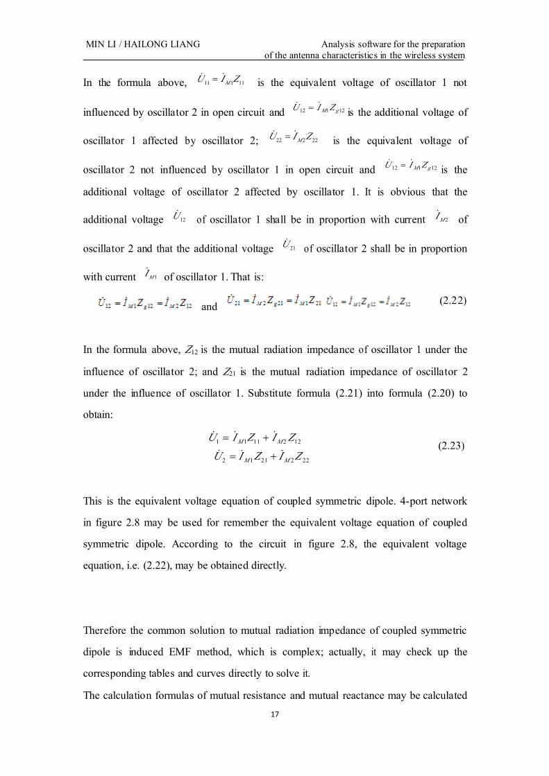
Substitute equation (2-4-3) into the formula above to obtain the equation below:

22212222122

12111211111

UUZIZIU

UUZIZIU

MgM

gMM

+=+=

+=+=(2.21)


17

In the formula above, 11111 ZIU M = is the equivalent voltage of oscillator 1 not

influenced by oscillator 2 in open circuit and 12112 gM ZIU = is the additional voltage of

oscillator 1 affected by oscillator 2; 22222 ZIU M = is the equivalent voltage of

oscillator 2 not influenced by oscillator 1 in open circuit and 12112 gM ZIU = is the

additional voltage of oscillator 2 affected by oscillator 1. It is obvious that the

additional voltage 12U of oscillator 1 shall be in proportion with current 2MI of

oscillator 2 and that the additional voltage 21U of oscillator 2 shall be in proportion

with current 1MI of oscillator 1. That is:

and (2.22)

In the formula above, Z12 is the mutual radiation impedance of oscillator 1 under the

influence of oscillator 2; and Z21 is the mutual radiation impedance of oscillator 2

under the influence of oscillator 1. Substitute formula (2.21) into formula (2.20) to

obtain:

2222112

1221111

ZIZIUZIZIU

MM

MM

+=

+=(2.23)

This is the equivalent voltage equation of coupled symmetric dipole. 4-port network

in figure 2.8 may be used for remember the equivalent voltage equation of coupled

symmetric dipole. According to the circuit in figure 2.8, the equivalent voltage

equation, i.e. (2.22), may be obtained directly.

Therefore the common solution to mutual radiation impedance of coupled symmetric

dipole is induced EMF method, which is complex; actually, it may check up the

corresponding tables and curves directly to solve it.

The calculation formulas of mutual resistance and mutual reactance may be calculated


18

by induced EMF method.

10

02

2

2

1

11112

10

02

2

2

1

11112

d)cos(

)cos(2)cos()cos(

|)]|(sin[30

d)sin(

)cos(2)sin()sin(

|)]|(sin[30

1

1

1

1

zrr

lrr

rr

zlX

zrr

lrr

rr

zlR

l

l

l

l

∫

∫

−

−

⎥⎦

⎤⎢⎣

⎡−+−=

⎥⎦

⎤⎢⎣

⎡−+−=

ββ

βββ

ββ

βββ

(2.24)

Figure.9 Mutual resistance and mutual reactance curve of coupled semi wave

symmetric dipole of coaxial line arrangement

Figure.9 shows the curve of variation of mutual resistance and mutual reactance of

coupled semi wave symmetric dipole (l1 = l2 = l = 0.25λ) of coaxial line arrangement

with distance. In the figure, s is the distance between two endpoints with which the

coupled symmetric dipole is confronting. The figure shows that amplitude of variation

of mutual resistance R12 and mutual reactance X12 is reduced gradually as the distance

s increases.


19

Figure.10 Mutual resistance and mutual reactance curves of coupled sine wave

symmetric dipole of level arrangement

If the distance between the two symmetric dipoles of level arrangement decreases

until to touch each other, a oscillator will be formed and then the self-radiation

impedance of the symmetric dipole is:

10 0

0

2

2

1

1111

10 0

0

2

2

1

1111

d)cos(

)cos(2)cos()cos(

)](sin[60

d)sin(

)cos(2)sin()sin(

)](sin[60

zrr

lrr

rr

zlX

zrr

lrr

rr

zlR

l

l

∫

∫

⎥⎦

⎤⎢⎣

⎡−+−=

⎥⎦

⎤⎢⎣

⎡−+−=

ββ

βββ

ββ

βββ

(2.25)

As for the sine wave symmetric dipole, self-radiation impedance is:

Z11 = R11 ＋ jX11 = 73.1 + j42.5 (Ω)

2.1.52.1.52.1.52.1.5 DirectivityDirectivityDirectivityDirectivity factorfactorfactorfactor andandandand gaingaingaingain coefficientcoefficientcoefficientcoefficient ofofofof antennaantennaantennaantenna

Directivity factor is a parameter representing the energy concentration degree of

antenna electromagnetic wave and is related to both directional characteristic and

impedance characteristic of antenna. [5]


20

Directivity factor is a parameter used to indicate the degree of electromagnetic wave

radiated by antenna intensively to a direction (i.e. sharpness of directional pattern). In

order to determine the directivity factors of antenna, an idea non-directional antenna

is generally used for a standard for comparison. [5]

The directivity factor of any directional antenna refers to the ratio of total radiant

power of non-directional antenna and total radiant power of the directional antenna

under the condition that the equal electric intensity is generated on the receiving point.

According to the definition above and because of unequal radiation intensities in

various directions of directional antenna, the directivity factors of antenna differ from

the different observation points, and the directivity factor is largest in the direction of

maximum radiated electric field. Except otherwise specified, the directivity factor of

the direction of maximum radiation is in general the directivity factor of directional

antenna. [6]

Definition 1: ratio of maximum radiation intensity and average radiation intensity.

Definition 2: ratio of power flux density in the direction of maximum radiation and

power flux density of ideal non-directional point source of antenna with the same

distance and radiation power；

Definition 3: ratio of the square of field intensity of in the direction of maximum

radiation and the square of ideal non-directional point source of antenna with the

same distance and radiation power;

000 )(),,(

)(),,(

20

2

00

maxPP

MMPP

MMPP rE

rErS

rSUU

D=== ΣΣΣ

===ϕθϕθ (2.26)

Substitute formula (1-4-25) and (1-4-5) into (1-4-27)) to obtain:

∫ ∫∫ ∫π ππ π

π=

π

=2

0 0

2

2max

2

0 0

max

d d sin),(

4

d d sin),(41 ϕθθϕθϕθθϕθ f

f

U

UD (2.27)


21

The normalized directivity function may also be used to calculate the directivity

factor.

∫ ∫π π

π=

2

0 0

2 d d sin),(

4

ϕθθϕθFD (2.28)

The radiation resistance may be used directly to calculate the directivity factor,

because that:

∫ ∫π πΣ

Σ π==

2

0 0

22

d d sin),(302ϕθθϕθf

IP

R (2.29)

A conclusion may be drawn that:

Σ

=Rf

D2

max120 (2.30)

The directivity factor may be calculated by effective length and radiation resistance,

because that:

2

maxee ll

fβ

λ=

π= (2.31)

We can deduce a conclusion:

in

2in

2 )(30)(30

ΣΣ

==Rl

Rl

D eeM ββ(2.32)

Note that the effective length, radiation resistance and fmax above are the electric

parameters with reference to the same current.

For example，the directivity factor D of current element = 2

2

)/(80)/(120

λπλπ

ll =1.5；

The directivity factor D of sine wave symmetric dipole =1.731120 2⋅ =1.64；

The directivity factor D of full wave symmetric dipole =199

2120 2⋅ =2.41.

Because that:


22

000 )(),,(

)(),,(

20

2

00

maxPP

MMPP

MMPP rE

rErS

rSUU

D=== ΣΣΣ

===ϕθϕθ

604

2404

221 2

02

22

02

0

20*

000ErrErEHEPP =⋅=⋅===Σ π

ππ

η

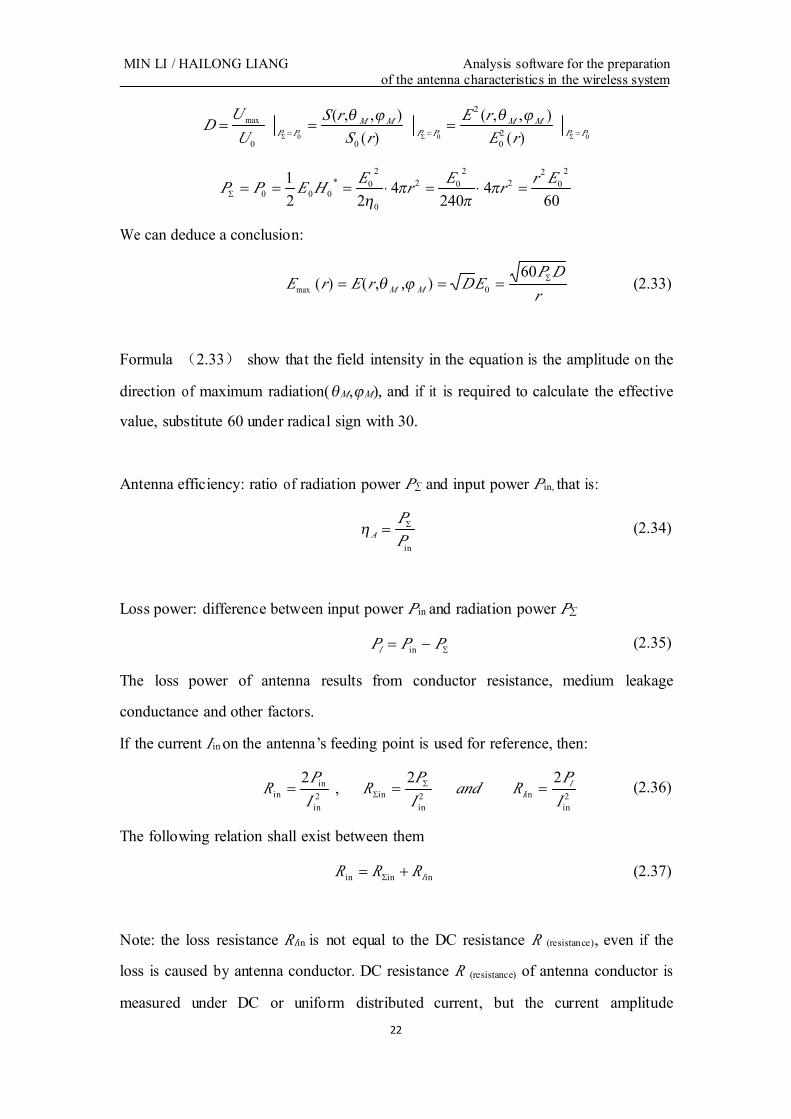
We can deduce a conclusion:

rDP

EDrErE MMΣ===

60),,()( 0max ϕθ (2.33)

Formula （2.33） show that the field intensity in the equation is the amplitude on the

direction of maximum radiation(θM,ϕM), and if it is required to calculate the effective

value, substitute 60 under radical sign with 30.

Antenna efficiency: ratio of radiation power P∑ and input power Pin, that is:

inPP

AΣ=η (2.34)

Loss power: difference between input power Pin and radiation power P∑

Σ−= PPPl in (2.35)

The loss power of antenna results from conductor resistance, medium leakage

conductance and other factors.

If the current I in on the antenna’s feeding point is used for reference, then:

2in

in2in

in2in

inin

2

2 ,

2IP

RandIP

RIP

R ll === Σ

Σ (2.36)

The following relation shall exist between them

ininin lRRR += Σ (2.37)

Note: the loss resistance R lin is not equal to the DC resistance R (resistance), even if the

loss is caused by antenna conductor. DC resistance R (resistance) of antenna conductor is

measured under DC or uniform distributed current, but the current amplitude


23

distribution I (z) on antenna in general is in-uniform.

Substitute formula (2.36) and (2.37) respectively into (2.34) to obtain:

inin

in

in

in

lA RR

RRR

+==

Σ

ΣΣη (2.38)

Two approaches to promote the antenna’s efficiency:

1. Reduce loss resistance R lin; and

2. Increase radiation resistance R∑in.

The gain coefficient of antenna is generally called also as maximum gain or antenna

gain. It refers to the ratio of the total input power of standard antenna (non-directional)

and the total input power of directional antenna under the condition that the equal

electric intensity is generated on a certain point in the direction of maximum field

intensity, which is called as the maximum gain coefficient of the antenna. It reflects

the effective utilization degree of radio-frequency power by antenna better than that of

antenna’s directivity factor. Mathematics may be used to deduce that the maximum

gain coefficient of antenna is equal to the antenna’s directivity factor multiplied by

antenna efficiency. [6]

The definition mode of antenna’s gain coefficient is quite similar to that of antenna’s

directivity factor.

000)(

),,()(

),,(20

2

00

max

PP

MM

PP

MM

PP inininrErE

rSrS

UU

G===

===ϕθϕθ (2.39)

Suppose that the input power of antenna can radiate to the free space completely, and

then the imaginary average radiation intensity converted from input power is:

π4'0

inPU = (2.40)

BecauseinPP

AΣ=η (2.41)


24

SoAA

UPU

ηπη0'

0 4== Σ

AA DUU

UU

G ηη ===0

max'0

max (2.42)

Therefore，gain coefficient G reflects the characteristics of antenna conversion and

radiation electromagnetic power more completely than that directivity factor D.

GPDPDP inAin ==Σ η , so the antenna’s radiation field on the direction of maximum

radiation may also be expressed as follows:

rGP

rDP

rE inmax

6060)( == Σ (2.43)

Where: F is the field intensity direction function.

2.2.2.2.2.2.2.2. MatlabMatlabMatlabMatlab backgroundbackgroundbackgroundbackground

Since the 1980s, electronic computers, especially the software of electronic computers

has achieved great development. In many software, mathematics technology

application software develop a school of their own. Until the mid of 1990s, there has

appeared on 30 several mathematics technology application software on international.

MATLAB in numerical calculation is the best of one, and Mathematical and Maple is

separated symbol computer software former two. In math technology application

software, MATLAB is a typical representative of the numerical computing, and may

be the first software which we come into contact with math technology application

software, in automatic control, communication, finance and other fields has a wide

range of application. MATLAB is released in the face of scientific computing,

visualization and interactive programming; the math works company by the U.S.

high-tech computing environment. It numerical analysis, matrix computation,

scientific data visualization, as well as nonlinear dynamic system modeling and


25

simulation, and many other powerful features are integrated in an easy to use

Windows environment, scientific research, engineering design and the need for

effective numerical calculation many fields of science to provide a comprehensive

solution, and largely out of the traditional non-interactive programming language

(such as C, Fortran), edit mode, and represents the advanced level of today's

international scientific computing software. [7]

ApplicationApplicationApplicationApplication developmentdevelopmentdevelopmentdevelopment softwaresoftwaresoftwaresoftware

The MATLAB product family can be used for the following work: [8]

Numerical Analysis

Numeric and symbolic computation

Engineering and scientific graphics

Control System Design and Simulation

Digital image processing techniques

Digital signal processing technology

Design and simulation of communication systems

The MATLAB has widely used range of applications, including signal and image

processing, communications, control system design, test and measurement, financial

modeling and analysis, and computational biology and other many applications.

Additional Toolbox (available separately dedicated set of MATLAB functions)

extends the MATLAB environment to solve particular types of problems in these

application areas.

2.32.32.32.3 MatlabMatlabMatlabMatlab GUIGUIGUIGUI introduceintroduceintroduceintroduce

The user interface (or interface) refers to the tools and methods of interaction between

man and machine (or program) can become a window to exchange information with

the computer, such as keyboard, mouse, track ball, microphone. Graphical user

interface (Graphical User Interfaces, GUI) is by the window, the cursor buttons,


26

menus, text and other objects (Objects) consisting of a user interface. Selected by

certain methods (such as a mouse and keyboard) to activate these graphic objects

enables a computer to produce a certain action or change, such as computing and

graphics.[9]

The user interface is the user and the hardware, software, interactive communications

intermediary, through the user interface; the user to the software instructions to

perform a function, the software uses the hardware, other software to implement the

directive, and results of the implementation in the form of graphics or text return to

the user. Early user interface is mostly the most typical form of a text-based DOS

system. The user to enter a command, the system by calling the software, hardware

resources to implement the directive, and the form of text to return to the results of the

implementation. Today, for most users, DOS (and similar user interface system)

seems to be a taboo enigmatic world, not only tedious, and the work efficiency is low;

people prefer a WYSIWYG user interface system, the graphical user interface

(Graphical user Interface, referred to as the GUI). The graphical user interface is

constituted by the window, the cursor keys, menus, text and other elements of the user

window, click on these elements, the user can very easily accomplish a function is

selected, the characteristics of this WYSIWYG especially good in drawing and other

applications.[10]

The graphical user interface program can be divided into two relatively independent

sub-modules, interface modules, and modules, interface modules to accept user input

and the input data and requests for action submitted to the work module; work module

is usually done in the background data processing tasks, and the results submitted to

the interface. Accordingly, GUI programming interface design and programming can

be divided into two parts. [11]


27

3.3.3.3. ProcessProcessProcessProcess andandandand ResultResultResultResult

3.13.13.13.1 TheTheTheThe antennaantennaantennaantenna parameterparameterparameterparameter calculationcalculationcalculationcalculation softwaresoftwaresoftwaresoftware designdesigndesigndesign

3.1.13.1.13.1.13.1.1 FlowFlowFlowFlow chartchartchartchart ofofofof designdesigndesigndesign aaaa GUIGUIGUIGUI interfaceinterfaceinterfaceinterface

MATLAB program design is relatively simple. The main purpose of GUI program is

to establish all kinds of interfaces to implement the function which is designed in the

beginning. The design gives scientific computing general appearance. As for each

block need to be refer to their corresponding function.

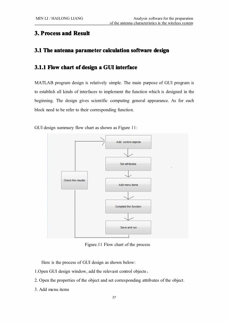
GUI design summary flow chart as shown as Figure 11:

Figure.11 Flow chart of the process

Here is the process of GUI design as shown below:

1.Open GUI design window, add the relevant control objects。

2. Open the properties of the object and set corresponding attributes of the object.

3. Add menu items


28

4. Write code to achieve the control function

5. Save and run the graphical user interface

6. Substituting numerical verify results

3.2The3.2The3.2The3.2The specificspecificspecificspecific processprocessprocessprocess

3.2.13.2.13.2.13.2.1 GenerationGenerationGenerationGeneration ofofofofMain-dialogMain-dialogMain-dialogMain-dialog boxboxboxbox

In this thesis student focus on using the matlab graphical user interface (GUI) to

accomplish the antenna parameter calculation software design. Before doing this

project need to know how to use the GUI to generate the user interface and How to

add the appropriate code in the CALLBACK function.

Select the default settings, click the OK button, dialog box appears. Add three buttons

in the dialog box. Double-click those three buttons. Changing the name of the three

buttons in the Property Inspector options, input impedance, mutual radiation

impedance, directional coefficient and gain coefficient. The Main dialog interface as

shown as Figure 12.


29

Figure 12 Matlab Main dialog interface

3.2.23.2.23.2.23.2.2 GenerationGenerationGenerationGeneration ofofofof sub-dialogsub-dialogsub-dialogsub-dialog boxboxboxbox

Similar step of the main dialogue, click the MATLAB GUIDE. But here should point

out that Storage path is the same as the main dialog. Generated three sub-dialog box

as shown below. Set sub-dialog box as calculate mutual radiation impedance Named

Mutal_impedance.fig. Add button and edit box and set them as in a correct way. The

results are shown in Figure 13.


30

Figure 13 Mutual radiation impedance interface

For the Mutal impedance sub-dialog box student could insert the variables to calculate

the mutal-radiation impedance. Using the formulas which are obtained from the

theoretical part. Set sub-dialog box; calculate the input impedance, named

mutal_impedance.fig. Similarly add buttons and edit boxes to adjust each tag of the

boxes into a correct way. The results are shown in Figure 13.


31

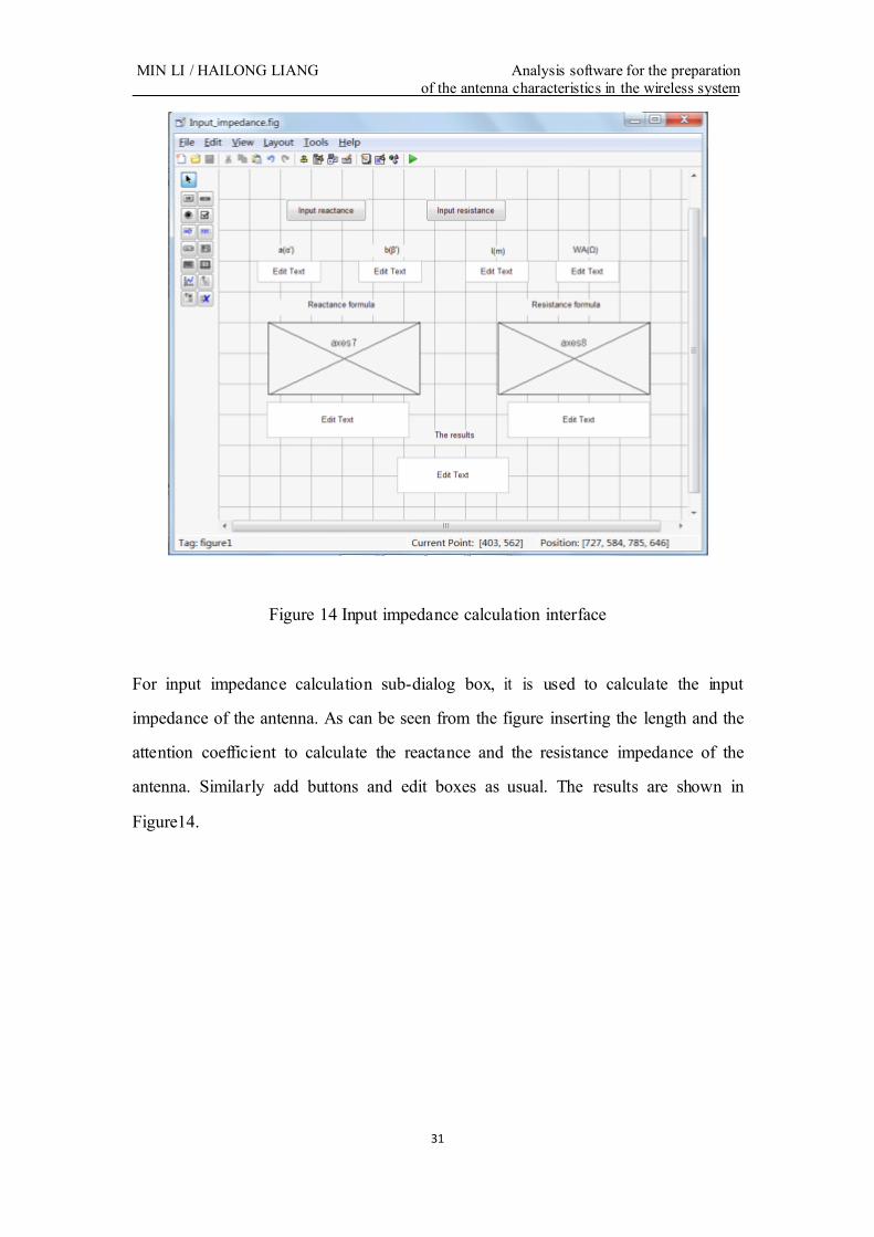
Figure 14 Input impedance calculation interface

For input impedance calculation sub-dialog box, it is used to calculate the input

impedance of the antenna. As can be seen from the figure inserting the length and the

attention coefficient to calculate the reactance and the resistance impedance of the

antenna. Similarly add buttons and edit boxes as usual. The results are shown in

Figure14.


32

Figure 15 The calculated directivity coefficient and gain coefficient interface

In this sub-dialog it contained the Directional factor and Gain factor calculation. First

integrate the wanted function to get the integration result A. Then insert the f(max)

and the antenna efficiency to get the result of Directional factor and Gain coefficient

of antenna. Similarly add buttons and edit boxes for each label corresponds to correct

box. The results are shown in Figure 15.


33

Figure 16 Input resistance curve interface plot

In this sub_dialog setting a plot to implement the input resistance curve with the

change of length/wavelength. Insert boxes include the attention coefficient, equivalent

impedance and the length/wavelength for the antenna. Similarly add buttons and edit

boxes to set them as in a correct way. The results are shown in Figure 16.


34

Figure 17 Input reactance curve interface plot

In this sub_dialog setting a plot to implement the reactance curve with the change of

length/wavelength. Insert boxes include the attention coefficient, equivalent average

resistance and the length/wavelength for the antenna. Similarly add buttons and edit

boxes to set them as in a correct way. The results are shown in Figure 17.


35

4.4.4.4. ResultResultResultResult

4.14.14.14.1 InterfaceInterfaceInterfaceInterface functionalfunctionalfunctionalfunctional verificationverificationverificationverification

Open the Main_dialog.fig file will show the figure below; this is the main dialog for

the whole interface.

Figure 18 Main interface dialog

In the result part for main dialog interface, students can click the bottom which

shown on the interface block to related interface. For example, if students click

input resistance plot bottom it will lead to the interface that plot the corresponding

figure of input resistance.


36

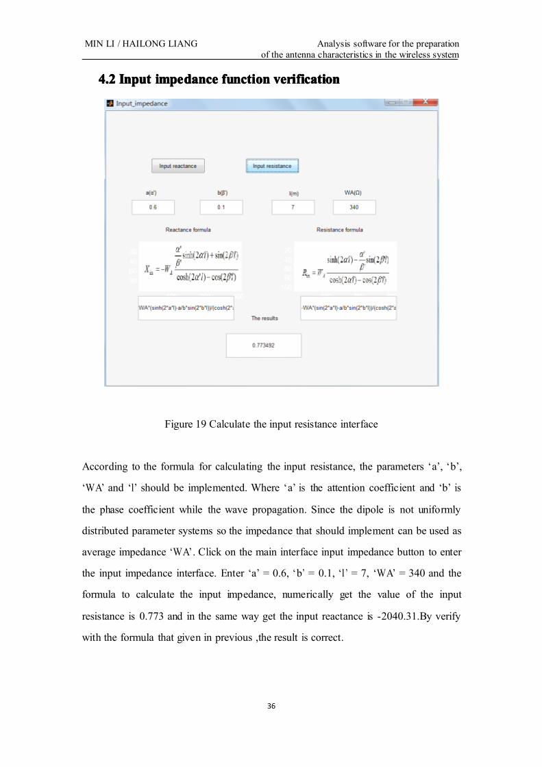
4.24.24.24.2 InputInputInputInput impedanceimpedanceimpedanceimpedance functionfunctionfunctionfunction verificationverificationverificationverification

Figure 19 Calculate the input resistance interface

According to the formula for calculating the input resistance, the parameters ‘a’, ‘b’,

‘WA’ and ‘l’ should be implemented. Where ‘a’ is the attention coefficient and ‘b’ is

the phase coefficient while the wave propagation. Since the dipole is not uniformly

distributed parameter systems so the impedance that should implement can be used as

average impedance ‘WA’. Click on the main interface input impedance button to enter

the input impedance interface. Enter ‘a’ = 0.6, ‘b’ = 0.1, ‘l’ = 7, ‘WA’ = 340 and the

formula to calculate the input impedance, numerically get the value of the input

resistance is 0.773 and in the same way get the input reactance is -2040.31.By verify

with the formula that given in previous ,the result is correct.


37

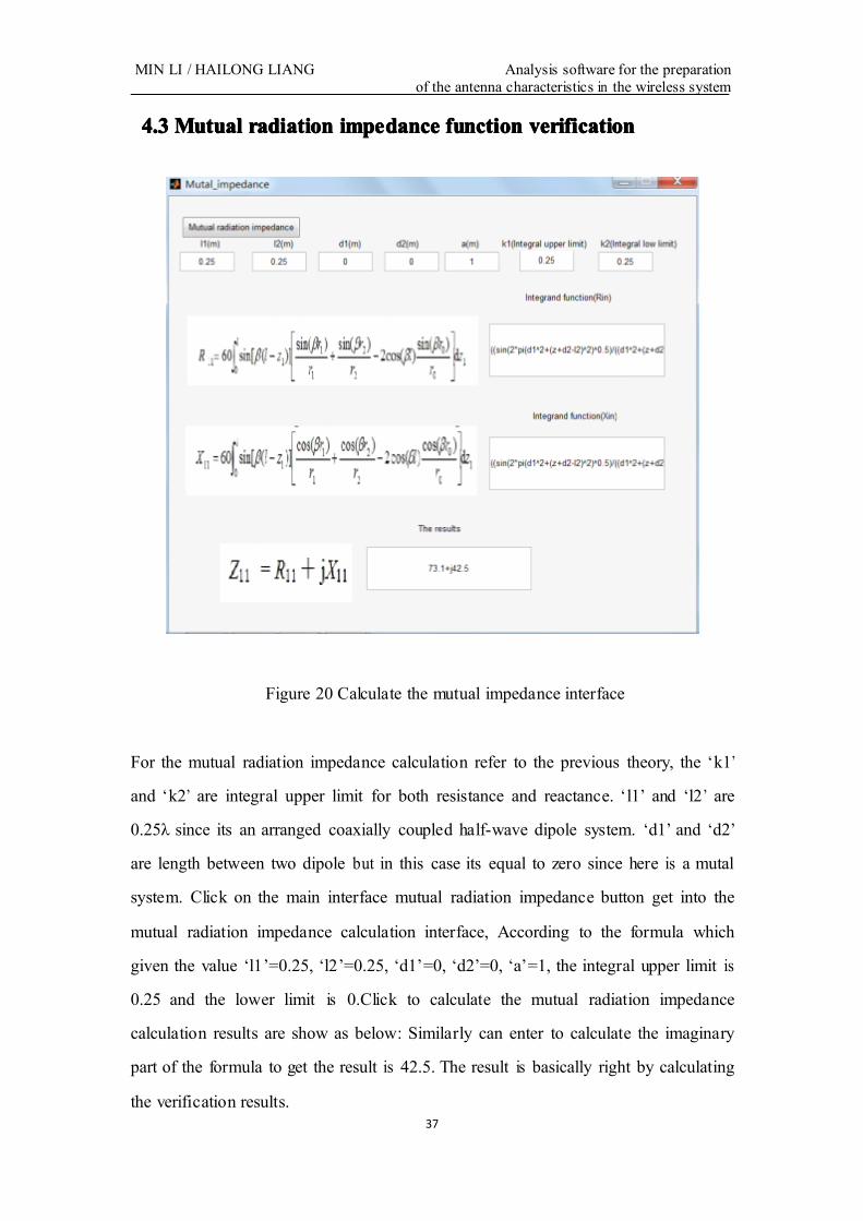
4.34.34.34.3 MutualMutualMutualMutual radiationradiationradiationradiation impedanceimpedanceimpedanceimpedance functionfunctionfunctionfunction verificationverificationverificationverification

Figure 20 Calculate the mutual impedance interface

For the mutual radiation impedance calculation refer to the previous theory, the ‘k1’

and ‘k2’ are integral upper limit for both resistance and reactance. ‘l1’ and ‘l2’ are

0.25λ since its an arranged coaxially coupled half-wave dipole system. ‘d1’ and ‘d2’

are length between two dipole but in this case its equal to zero since here is a mutal

system. Click on the main interface mutual radiation impedance button get into the

mutual radiation impedance calculation interface, According to the formula which

given the value ‘l1’=0.25, ‘l2’=0.25, ‘d1’=0, ‘d2’=0, ‘a’=1, the integral upper limit is

0.25 and the lower limit is 0.Click to calculate the mutual radiation impedance

calculation results are show as below: Similarly can enter to calculate the imaginary

part of the formula to get the result is 42.5. The result is basically right by calculating

the verification results.


38

4.44.44.44.4 TheTheTheThe directionaldirectionaldirectionaldirectional coefficientcoefficientcoefficientcoefficient andandandand thethethethe validationvalidationvalidationvalidation ofofofof thethethethe gaingaingaingain

coefficientcoefficientcoefficientcoefficient

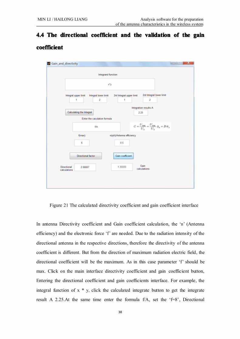
Figure 21 The calculated directivity coefficient and gain coefficient interface

In antenna Directivity coefficient and Gain coefficient calculation, the ‘n’ (Antenna

efficiency) and the electronic force ‘f ’ are needed. Due to the radiation intensity of the

directional antenna in the respective directions, therefore the directivity of the antenna

coefficient is different. But from the direction of maximum radiation electric field, the

directional coefficient will be the maximum. As in this case parameter ‘f ’ should be

max. Click on the main interface directivity coefficient and gain coefficient button,

Entering the directional coefficient and gain coefficients interface. For example, the

integral function of x * y, click the calculated integrate button to get the integrate

result A 2.25.At the same time enter the formula f/A, set the ‘f=8’, Directional


39

coefficient can be calculated for 2.6667, set ‘n=0.5’, Computable gain coefficient for

1.3333.The result is shown in Figure 21.

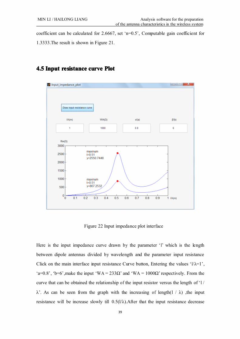
4.54.54.54.5 InputInputInputInput resistanceresistanceresistanceresistance curvecurvecurvecurve PlotPlotPlotPlot

Figure 22 Input impedance plot interface

Here is the input impedance curve drawn by the parameter ‘l’ which is the length

between dipole antennas divided by wavelength and the parameter input resistance

Click on the main interface input resistance Curve button, Entering the values ‘l/λ=1’,

‘a=0.8’, ‘b=6’,make the input ‘WA = 233Ω’ and ‘WA = 1000Ω’ respectively. From the

curve that can be obtained the relationship of the input resistor versus the length of ‘l /

λ’. As can be seen from the graph with the increasing of length(l / λ) ,the input

resistance will be increase slowly till 0.5(l/λ).After that the input resistance decrease


40

and then increase a bit. At the same time maximum point and the other coordinate can

also be found on the curve in Figure 22.

4.64.64.64.6 InputInputInputInput reactancereactancereactancereactance CurveCurveCurveCurve PlotPlotPlotPlot

Figure 23 Input reactance plot interface

Here is the input reactance curve plot by the parameter ‘l’ which is the length between

dipole antennas divided by wavelength and the parameter input reactance. Click on

the main interface input reactance Curve button to get into the input curve drawing

interface. Entering ‘l/λ=1’, ‘a=0.8’, ‘b=6,’ ‘WA=340’.From the input reactance curve

can be obtained with the relationship of the length( l / λ).As can be seen from this

graph with the increasing by the length(l/λ) the input reactance won’t change after a

certain point. This is good because it can get rid of the reactance part to reduce

interference. Also the maximum value can be found on the curve shown as Figure 23.


41

5.5.5.5. DiscussionDiscussionDiscussionDiscussion

This design is the first time we preparation software interface by using Matlab GUI.

In this project students investigate the antenna characteristics and meet the design

requirements which is corresponding with the antenna theory by using the design of

Matalb GUI interface. At the beginning students supposed to implement this design

by using VC++, but students found that there is too hard to insert the formula which

obtained in the calculation part to compile. And another problem is difficult to

carrying out the syntax check with matching brackets, expression evaluates. This is

the main reason that students choose Matlab GUI interface to achieve the goal at last.

In the matlab GUI designing it is successful realization of the calculation of the

coefficients of antenna. In mutual impedance interface it works with entering the

formula to calculate the value by only press the pushbutton .And in the input

reactance/resistance part it would be easy to achieve the function by using the

pushbutton. As for the input impedance plot/input reactance plot students set the

function to plot the figure with corresponding to the theory.


42

6.6.6.6. ConclusionConclusionConclusionConclusion

The purpose of this paper is design an initial platform which can be used for

education. Students would have learned more knowledge about the antenna system

and how to calculate the parameters of antenna coefficient by using the interface

function of Matlab. Matlab GUI can simplify the complex calculation process by

given the values of needed parameters and formulas. Every interface are

corresponding to its Callback function .In this paper we give a depth discussion and

description of diploe antenna’s input impedance and the antenna coefficient, such as

input impedance, input reactance and mutual impedance of antennas. For this project

it is just a initial design for the interface and we believe students can improve this in

different conditions and to get the results better in the future.


43

7.7.7.7. Reference:Reference:Reference:Reference:

[1] Jin Lihong, 17-18 July 2011, Application of MATLAB Software for Linear

Algebra, pp: 1-3

[2] Owczarek, M.S. , Inst. of Electron., Lodz Tech. Univ., Poland Langer,

M. ; Wozny, J. ; Nowak, J. 28-28 Feb. 2004,Design of graphical user interface (GUI)

for analog EDA tool, PP: 560 – 562

[3] S. Lee, Y. Li, V. Kapila, 2004. “Development of a Matlab-Based Graphical

User Interface Environment for PICMicrocontroller Projects”, The 2004 American

Society for Engineering Education Annual Conference & Exposition.

[4] N. Aliane, July 2009. “Matlab/Simulink-Based Interactive Module for Servo

Systems Learning”, IEEE Transactions onEducation, Volume: 53, Issue: 2, pp. 265 –

271.

[5] Bachiller, C. Departamento de Comunicaciones, Univ. Politecnica de

Valencia Esteban, H. ; Cogollos, S. ; San Blas, A. ; Boria, V.E. , 2002, Teaching of

wave propagation phenomena using Matlab GUIs at the Universidad Politecnica of

Valencia, PP: 696 – 699, vol.1

[6] Kevanishvili, G.S. Georgian Tech. Univ., Tbilisi, Georgia Kotetishvili,

K.V. ; Vashadze, G.K. ; Bolkvadze, D.R. 2002 A theory of symmetric dipole formed

of thin rectangular metallic plates,PP:::: 21 - 24

[7] Lepeltier, Ph. Floc'h, J.M. ; Citerne, J. ; Piton, G. , Sept. 1986, Self Impedance

and Radiation Patterns of the Electromagnetically Coupled Microstrip Dipole, PP:

649 – 654


44

[8] Trainotti, V. Fac. of Eng., Univ. of Buenos Aires, Buenos Aires,

Argentina Figueroa, G. Sept. 2010, Vertically Polarized Dipoles and Monopoles,

Directivity, Effective Height and Antenna Factor,VOL: 56, PP: 379 - 409

[9] E. A. Laport, (1952), Radio Antenna Engineering. NewYork: McGraw-Hill,C.

A. Balanis, “Antenna Theory: A Review,” Proc. IEEE, Vol. 80, No. 1, pp. 7–23

[10] Mingyang Li, Liu Min, Yang Fang, Aug.2011, Antenna design, Pubishing

House of electronics Industry, BEIJING, PP: 1-8

[11] Ahmed A. Klshk, 2005, A.Balanis, Antenna theory, analysis and design,

Third edition, John Wiley & Sons INC., Publication, PP: 1-65


45

8.8.8.8.AppendixAppendixAppendixAppendix

CodeCodeCodeCode part:part:part:part:functionvarargout = untitled4(varargin)

gui_Singleton = 1;

gui_State = struct('gui_Name',

'gui_Singleton',

'gui_OpeningFcn',

'gui_OutputFcn',

'gui_LayoutFcn',

'gui_Callback',

ifnargin&&ischar(varargin1)

gui_State.gui_Callback = str2func(varargin1);

end

ifnargout

[varargout1:nargout] = gui_mainfcn(gui_State, varargin:);

else

gui_mainfcn(gui_State, varargin:);

end

8.18.18.18.1 MainMainMainMain dialoguedialoguedialoguedialogue codecodecodecode

symsz;

a= str2double(get(handles.edit1, 'String'));

b=str2double(get(handles.edit2, 'String'));

l=str2double(get(handles.edit3, 'String'));

WA=str2double(get(handles.edit4, 'String'));

e=get(handles.edit6,'string');


46

z1=e;

m=eval(z1);

set(handles.edit7,'string',m)

symsz;



l=str2double(get(handles.edit3, 'String'));



z1=e;

m=eval(z1);


8.28.28.28.2 MutualMutualMutualMutual radiationradiationradiationradiation impedanceimpedanceimpedanceimpedance

symsz;

l1= str2double(get(handles.edit1, 'String'));

l2=str2double(get(handles.edit2, 'String'));

d1=str2double(get(handles.edit3, 'String'));

d2=str2double(get(handles.edit4, 'String'));


k1=str2double(get(handles.edit6, 'String'));

k2=str2double(get(handles.edit7, 'String'));


z1=int(e,z,k1,k2);

m=eval(z1);

set(handles.edit9,'string',m);


47

8.38.38.38.3 TheTheTheThe calculatedcalculatedcalculatedcalculated directivitydirectivitydirectivitydirectivity coefficientcoefficientcoefficientcoefficient andandandand gaingaingaingain coefficientcoefficientcoefficientcoefficient

symsxy



c=str2double(get(handles.edit4, 'String'));

d=str2double(get(handles.edit5, 'String'));


z=int(int(e,y,c,d),a,b);

m=eval(z);

set(handles.edit6,'string',m);

AddAddAddAdd thethethethe followingfollowingfollowingfollowing codecodecodecode inininin calculatingcalculatingcalculatingcalculating thethethethe directionaldirectionaldirectionaldirectional coefficientcoefficientcoefficientcoefficient CallbackCallbackCallbackCallback

functionfunctionfunctionfunction：

A=str2double(get(handles.edit6, 'String'));

f=str2double(get(handles.edit7, 'String'));


k=e;

m=eval(k);


n=str2double(get(handles.edit8, 'String'));

w=str2double(get(handles.edit9, 'String'));

s=n*w;

set(handles.edit11,'string',s);


48

8.48.48.48.4 inputinputinputinput resistanceresistanceresistanceresistance curvecurvecurvecurve

l= str2double(get(handles.edit1, 'String'));


a=str2double(get(handles.edit3, 'String'));


t=0:0.01:l;

y=WA*(sinh(2*a*t)-(a/b)*sin(2*b*t))./(cosh(2*a*t)-cos(2*b*t));

[y_max,i_max]=max(y);

t_text=['t=',num2str(t(i_max))];

y_text=['y=',num2str(y_max)];

max_text=char('maxinum' ,t_text,y_text);

plot(t,y)

holdon

plot(t,zeros(size(t)),'k')

plot(t(i_max),y_max,'r.','MarkerSize',20);

text(t(i_max)-0.3,y_max-0.05,max_text);

8.58.58.58.5 DrawDrawDrawDraw inputinputinputinput reactancereactancereactancereactance curvecurvecurvecurve

l= str2double(get(handles.edit1, 'String'));


a=str2double(get(handles.edit3, 'String'));


t=0:0.01:l;

y=-WA*((a/b)*sinh(4*pi*t)+sin(4*pi*t))./(cosh(4*pi*t)-cos(4*pi*t));

[y_max,i_max]=max(y);

t_text=['t=',num2str(t(i_max))];

y_text=['y=',num2str(y_max)];


49

max_text=char('maxinum' ,t_text,y_text,wa_text);

plot(t,y)

holdon

plot(t,zeros(size(t)),'k')

plot(t(i_max),y_max,'r.','MarkerSize',20);

text(t(i_max)-0.3,y_max-0.05,max_text);

Analysis software for the preparation of the antenna

Documents

Transcript of Analysis software for the preparation of the antenna