Analysis of Variance€¦ · • Analysis of variance compares two or more populations of interval...
223
Analysis of Variance
Transcript of Analysis of Variance€¦ · • Analysis of variance compares two or more populations of interval...

Analysis of Variance

• What is ANOVA?
• When is it useful?
• How does it work?
• Some Examples

Introduction
• Analysis of variance compares two or more
populations of interval data.
• Specifically, we are interested in determining whether
differences exist between the population means.
• The procedure works by analyzing the sample
variance.

Variables
1. Dependent variable: Metric data (Continuous)
Ex. Sales, Profit, Market share Age, Height etc.
2. Independent variable: Non-metric data(categorical)
Ex. Sales promotion(High, Medium and Low),
Region ( Delhi, Lucknow and Bhopal)

Questionnaire
• Metric data: Ex. The sales of this organization is ……,
I am satisfied the quality of product
1………...2………..3……...4……………5 Strongly disagree Disagree Neutral Agree Strongly agree
• Non-metric data: Ex. In-store promotion-
a) High,
b) Medium
c) Low

Data
• Any data set has variability
• Variability exists within groups…
• and between groups

Question that ANOVA allows us to answer : Is
this variability significant, or merely by chance?
• The difference between variation within a group and variation
between groups may help us determine this. If both are equal it
is likely that it is due to chance and not significant.
• H0: Variability within groups = variability between groups,
this means that
• Ha: Variability within groups does not = variability between
groups, or,

Assumptions
• Normal distribution
• Variances of dependent variable are equal in
all populations
• Random samples; independent scores

One-Way ANOVA
• One factor (manipulated variable)
• One response variable
• Two or more groups to compare

Usefulness
• Similar to t-test
• More versatile than t-test
• Compare one parameter (response variable) between
two or more groups

For instance, ANOVA Could be Used to:
• Compare heights of plants with and without galls
• Compare birth weights of deer in different geographical
regions
• Compare responses of patients to real medication vs. placebo
• Compare attention spans of undergraduate students in different
programs at PC.

Why Not Just Use t-tests?
• Tedious when many groups are present
• Using all data increases stability
• Large number of comparisons some may

Remember that…
• Standard deviation (s)
n
s = √[(Σ (xi – X)2)/(n-1)]
i = 1
• In this case: Degrees of freedom (df)
df = Number of observations or groups - 1

Notation
• k = Number of groups
• n = Number observations in each group
• Yi = Individual observation
• Yij = ith observation in the jth category
• SS = Sum of Squares
• MS = Mean of Squares
• F = MSbetween/ MSerror

Calculation of SS Values

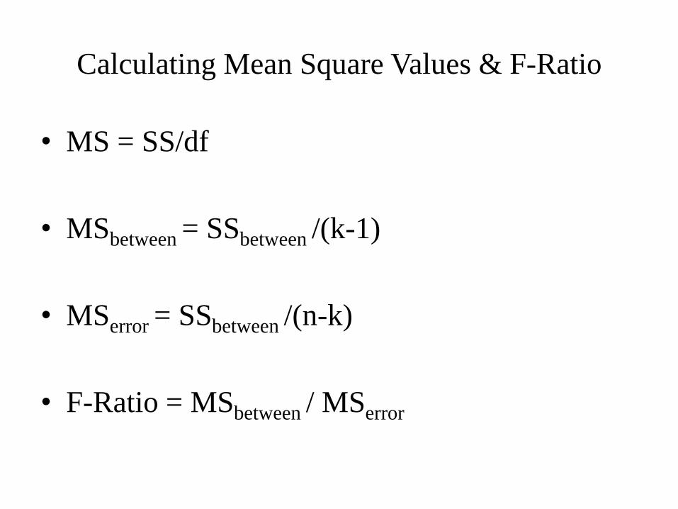
Calculating Mean Square Values & F-Ratio
• MS = SS/df
• MSbetween = SSbetween /(k-1)
• MSerror = SSbetween /(n-k)
• F-Ratio = MSbetween / MSerror

Total sum of squares • SSy = SSbetween + SSwithin
or
• SSy = SSx + SSerror
Where
SSy = The total variation in Y
SSbetween = Variation between the categories of X
SSwithin = Variation in Y related to the variation within each
category of X
Calculating Mean Square Values & F-Ratio
• MS = SS/df
• MSbetween = SSbetween /(k-1)
• MSerror = SSbetween /(n-k)
• F-Ratio = MSbetween / MSerror

Hypothesis Testing & Significance Levels

F-Ratio = MSbetween / MSerror
• If:
– The ratio of Between-Groups MS: Within-Groups MS is
LARGE reject H0 there is a difference between
groups
– The ratio of Between-Groups MS: Within-Groups MS is
SMALLdo not reject H0 there is no difference between
groups

p-values
• Use table in stats book to determine p
• Use degree of freedom for numerator and
denominator
• Choose level of significance
• If Fcalculated > Fcritical value, reject the null hypothesis
(for one-tail test)

• Example
– An experiment in which a major department store chain wanted to
examine the effect of the level of in -store promotion.
– The experimenter wants to know the impact of the in -store
promotion on sales.
– In store promotion was varied at three levels:
1. High promotion.
2. Medium promotion.
3. Low promotion.
One Way Analysis of Variance

Data…..
Metric data: Sales(Continuous variable)
1- to- 10 scale used, higher numbers denote higher sales.
1…….2…….3……4…….5……..6……7…..8……..9……10
Low High
Non- metric data: In- store promotion(Categorical variable)
High promotion-1
Medium promotion-2
Low promotion-3

Effect of In-store promotion on sales
Store No. Level of In- store promotion
High Medium Low
1 10 8 5
2 9 8 7
3 10 7 6
4 8 9 4
5 9 6 5
6 8 4 2
7 9 5 3
8 7 5 2
9 7 6 1
10 6 4 2
Column total 83 62 37
Category means: 83/10= 8.3 62/10= 6.2 37/10= 3.7
Grand means, ( 83+62+37)/30 = 6.067

• Suppose that only one factor, namely in-store
promotion, was manipulated. The department store is
attempting to determine the effect of in- store
promotion(X) on sales(Y).
• The null hypothesis is that the category means
are equal:
H0: m1 = m2= m3
H1: At least two means differ

To test the null hypothesis, the various sums of
squares are computed:
ANOVA Calculations: Sums of Squares
SSy =
(10 - 6.067)2 + (09 - 6.067)2 +(10 - 6.067)2 + (08 - 6.067)2 + (09 - 6.067)2 +
(08 - 6.067)2 + (09 - 6.067)2 + (07 - 6.067)2 + (07 - 6.067)2+ (06 -6.067)2 +
(08 - 6.067)2 + (08 - 6.067)2 + (07 - 6.067)2 + (09 - 6.067)2 + (06 -6.067)2 +
(04 - 6.067)2 + (05 - 6.067)2 + (05 - 6.067)2 + (06 - 6.067)2 + (04 -6.067)2 +
(05 - 6.067)2 + (07 - 6.067)2 + (06 - 6.067)2 + (04 - 6.067)2 + (05 -6.067)2 +
(2 - 6.067)2 + (3 - 6.067)2 + (2 - 6.067)2 + (1 - 6.067)2 + (2 - 6.067)2

Continued….
SSy =
(3.933)2 + (2.933)2 + (3.933)2 + (1.933)2 + (2.933)2 + (1.933)2 +
(2.933)2 + (0.933)2 + (0.933)2 + (-0.067)2 + (1.933)2 + (1.933)2 +
(0.933)2 + (2.933)2 + (-0.067)2 + (-2.067)2 + (-1.067)2 + (-1.067)2 +
(-0.067)2 + (-2.067)2 + (-1.067)2 + (0.933)2 + (-0.067)2 + (-2.067)2 +
(-1.067)2 +(-4.067)2 +(-3.067)2 +(-4.067)2 +(-5.067)2 +(-4.067)2
= 185.867

Sum of Square between the categories
SSx = 10(8.3 - 6.067)2 + 10(6.2 - 6.067)2+ 10(3.7 - 6.067)2
= 10 (2.233)2 + 10 (0.133)2 +10 (-2.367)2
= 106.067

Sum of square within the categories
SSerror =
(10-8.3)2 + (09-8.3)2 + (10-8.3)2 + (08-8.3)2 + (09-8.3)2 + (08-8.3)2 +
(09-8.3)2+ (07-8.3)2 + (07-8.3)2 + (06-8.3)2 + (08-6.2)2 + (08-6.2)2 +
(07-6.2)2+ (09-6.2)2 + (06-6.2)2 + (04-6.2)2 + (05-6.2)2 + (05-6.2)2 +
(06-6.2)2+(04-6.2)2+ (05-3.7)2 + (07-3.7)2 + (06-3.7)2 + (04-3.7)2 +
(05-3.7)2 +(02-3.7)2 +(03-3.7)2 +(02-3.7)2 +(01-3.7)2 +(02-3.7)2

Continued….
SSerror =
(1.7)2 + (0.7)2 + (1.7)2 + (-0.3)2 + (0.7)2 + (-0.3)2 + (0.7)2 + (-1.3)2
+ (-1.3)2 + (-2.3)2 + (1.8)2 + (1.8)2 + (0.8)2 + (2.8)2 + (-0.2)2 + (-2.2)2
+ (-1.2)2 + (-1.2)2 + (-0.2)2 + (-2.2)2 + (1.3)2 + (3.3)2 + (2.3)2 + (0.3)2
+ (1.3)2 + (-1.7)2 + (-0.7)2 + (-1.7)2 + (-2.7)2 + (-1.7)2
= 79.80

It can be verified that
SSy = SSx + SSerror
As follows: 185.867 = 106.067 +79.80
The strength of the effects of X on Y are measured as follows:
h2SSx / SSy
= 106.067/185.867
= 0.571
57.percent of the variation in sales (Y) is accounted for by
in-store promotion (X), indication a modest effect.

ANOVA Calculations: Mean Squares & Fcalc
MSx = SSx / (k-1)
= 106.067/2 = 53.033
MSerror = SSerror /(N-k)
= 79.800/27 = 2.956
Fcalc = MSx / MSerror
= 17.944
Fcrit = Fa,k-1,n-k = F.05,2,27 = 3.35

F-table portion with = .05
1
2 1 2 3 4 5 6 .... 60 1 161.4 199.5 215.7 224.6 230.2 234.0 .... 252.2 2 18.51 19.00 19.16 19.25 19.30 19.33 .... 19.48 3 10.13 9.55 9.28 9.12 9.01 8.94 .... 8.57 . . . . . . . .... . . . . . . . . .... . 20 4.35 3.49 3.10 2.87 2.71 2.60 .... 1.95 . . . . . . . .... . 27 . . . . . . .... . 30 4.17 3.32 2.92 2.69 2.53 2.42 .... 1.74 40 4.08 3.23 2.84 2.61 2.45 2.34 .... 1.64
3.35
2
27

One -way ANOVA: Effect of In store promotion
on store sales
Source of df SS MS Fcalc Fcrit
Variation
Between 2 106.067 53.033 17.944 3.35 Groups (In-store promotion)
Within 27 79.800 2.956 Groups (Error)
Total 29 185.867
Since Fcalc > Fcrit there is strong evidence for a difference
between Groups means.

Conclusion……
We see that for 2 and 27 degree of freedom, the critical value
of F is 3.35 for = 0.05. the calculated value of F is greater
than the critical value, we reject the null hypothesis. We
conclude that the population means for the three levels of in-
store promotion are indeed different. the relative magnitude of
the means for three categories indicate that a high level of in-
store promotion leads to significantly higher sales.

ANOVA - a recapitulation.
• This is a parametric test, examining whether the means differ
between 2 or more populations.
• It generates a test statistic F, which can be thought of as a
signal-noise ratio. Thus large Values of F indicate a high
degree of pattern within the data and imply rejection of H0.
• It is thus similar to the t test - in fact ANOVA on 2 groups is
equivalent to a t test [F = t2 ]

One way ANOVA’s limitations
• This technique is only applicable when
there is one treatment used.
• Note that the one treatment can be at 3, 4,…
many levels.

N-way analysis of variance
or
Randomised Block Design
or
Two - Way Analysis of Variance

Two- Way Analysis of Variance
• What is 2-Way ANOVA?
• When is it useful?
• How does it work?
• Some Examples

Variables
1. Dependent variable: Metric data (Continuous)
Ex. Sales, Profit, Market share ,Age, Height etc.
2. Independent variable: Non-metric data(categorical)
Ex. Sales promotion(High, Medium and Low),
Coupon( Rs.20, not Rs. 20)
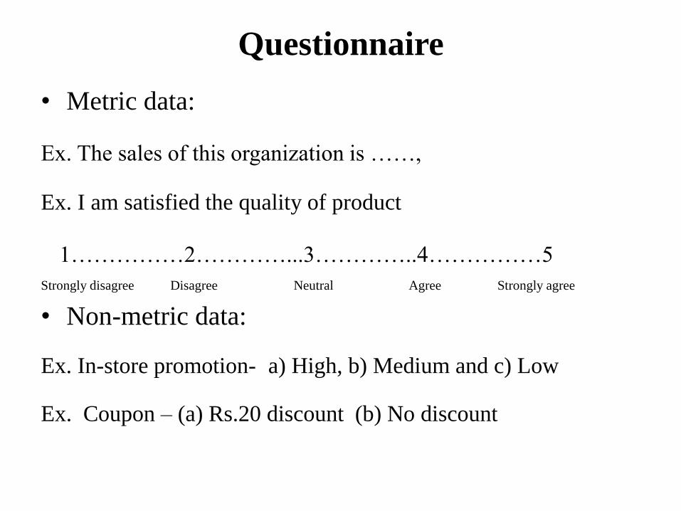
Questionnaire
• Metric data:
Ex. The sales of this organization is ……,
Ex. I am satisfied the quality of product
1……………2…………...3…………..4……………5
Strongly disagree Disagree Neutral Agree Strongly agree
• Non-metric data:
Ex. In-store promotion- a) High, b) Medium and c) Low
Ex. Coupon – (a) Rs.20 discount (b) No discount

Data
• Any data set has variability
• Variability exists within groups…
• and between groups

Two-way Analysis of Variance
• Two-way ANOVA is a type of study design with one
numerical outcome variable and two categorical explanatory
variables.
• Example – In a completely randomised design we may wish to
compare outcome by categorical variables. Subjects are
grouped by one such factor and then randomly assigned one
treatment.
• Technical term for such a group is block and the study design
is also called randomised block design

Two- Way Analysis of Variance
• Blocks are formed on the basis of expected homogeneity of
response in each block (or group).
• Randomised block design is a more robust design than the
simple randomised design.
• The investigator can take into account simultaneously the
effects of two factors on an outcome of interest.
• Additionally, the investigator can test for interaction, if any,
between the two factors.

Steps in Planning a Two- Way Analysis of Variance
1) Subjects are randomly selected to constitute a random
sample.
2) Subjects likely to have similar response (homogeneity) are
put together to form a block.
3) To each member in a block intervention is assigned such that
each subject receives one treatment.
4) Comparisons of treatment outcomes are made within each
block

Two- Way Analysis of Variance
In marketing research, one is often concerned with the effect of
more than one factor simultaneously.
For example:
1. How do advertising levels (high, medium, and low) interact with
price levels (high, medium, and low) to influence a brand's sale?

Continued….
2. Do educational levels (less than high school, high school
graduate, some college, and college graduate) and age (less
than 35, 35-55, more than 55) affect consumption of a brand?
3. What is the effect of consumers' familiarity with a department
store (high, medium, and low) and store image (positive,
neutral, and negative) on preference for the store?

Two -way Analysis of Variance
Consider the simple case of two factors X1 and X2 having
categories k1 and k2. The total variation in this case is partitioned
as follows:
SStotal = SS due to X1 + SS due to X2 + SS due to interaction of X1 and X2 + SSwithin
or
SSy = SSx1 + SSx2
+ SSx1x2 + SSerror

Two -way Analysis of Variance

Notation k1, k2 = Number of groups
n = Number observations in each group
Yijn = Score for participants n within group that correspond to category i of the factor-x1 and category j of the factor -x2 .
• SS = Sum of Squares
• MS = Mean of Squares
• F = MSbetween/ MSerror

Continue….
The strength of the joint effect of two factors, called the overall
effect, or multiple 2, is measured as follows:
(SSx1 + SSx2
+ SSx1x2)/ SSyMultiple 2 = h
h

Two -way Analysis of Variance
The significance of the overall effect may be tested by an F test, as follows
where
dfn = degrees of freedom for the numerator
= (k1 - 1) + (k2 - 1) + (k1 - 1) (k2 - 1)
= k1k2 - 1
dfd = degrees of freedom for the denominator
= N - k1k2
MS = mean square
F = (SSx 1
+ SSx 2 + SSx 1x 2
)/dfnSSerror/dfd
= SSx 1,x 2,x 1x 2
/ dfn
SSerror/dfd
= MSx 1,x 2,x 1x 2
MSerror

Two -way Analysis of Variance
If the overall effect is significant, the next step is to examine the
significance of the interaction effect. Under the null hypothesis of no
interaction, the appropriate F test is:
where
dfn = (k1 - 1) (k2 - 1)
dfd = N - k1k2
F = SSx 1x 2
/dfnSSerror/dfd
= MSx 1x 2
MSerror

Two -way Analysis of Variance
The significance of the main effect of each factor may be tested as
follows for X1:
where
dfn = k1 - 1
dfd = N - k1k2
F = SSx 1
/dfnSSerror/dfd
= MSx 1
MSerror

• Example:
An experiment in which a major department store chain wanted to examine the
effect of the level of in -store promotion and couponing on store sales.
In store promotion was varied at three levels:
1. High promotion.
2. Medium promotion and
3. Low promotion.
Coupon was manipulated at two levels :
1. Rs.20 discount and
2. No discount
Two-way Analysis of Variance

Data…..
A. Metric data: Sales(Continuous variable)
1- to- 10 scale used, higher numbers denote higher sales.
1…….2…….3……4…….5……..6………7……..8……..9……..10.
Low High
B. Non- metric data(Factor-1): In- store promotion(Categorical variable)
1. High promotion
2. Medium promotion
3. Low promotion
Non- metric data (Factor-2): Couponing(Categorical variable)
1. Rs.20 discount
2. No discount

Effect of In-store promotion on store sales
Store No. Level of In- store promotion
High Medium Low
1 10 8 5
2 9 8 7
3 10 7 6
4 8 9 4
5 9 6 5
6 8 4 2
7 9 5 3
8 7 5 2
9 7 6 1
10 6 4 2
Column total 83 62 37
Category means: 83/10= 8.3 62/10= 6.2 37/10= 3.7
Grand means, ( 83+62+37)/30 = 6.067

Effect of Coupon on store sales
Store No. Level of Coupon
Discount No-discount
1 10 8
2 9 9
3 10 7
4 8 7
5 9 6
6 8 4
7 8 5
8 7 5
9 9 6
10 6 4
11 5 2
12 7 3
13 6 2
14 4 1
15 5 2
Category means:
7.4 4.733
Grand means,
(111+ 71)/30 = 6.067

Two -way Analysis of Variance
• In this case two - factors, namely in-store promotion,
and Coupon were manipulated. The department store
is attempting to determine the effect of in- store
promotion(Xp) and coupon(Xc) on sales(Y).

The various sums of squares are computed:
SSy =
(10 - 6.067)2 + (09 - 6.067)2 +(10 - 6.067)2 + (08 - 6.067)2 + (09 - 6.067)2 +
(08 - 6.067)2 + (09 - 6.067)2 + (07 - 6.067)2 + (07 - 6.067)2+ (06 -6.067)2 +
(08 - 6.067)2 + (08 - 6.067)2 + (07 - 6.067)2 + (09 - 6.067)2 + (06 -6.067)2 +
(04 - 6.067)2 + (05 - 6.067)2 + (05 - 6.067)2 + (06 - 6.067)2 + (04 -6.067)2 +
(05 - 6.067)2 + (07 - 6.067)2 + (06 - 6.067)2 + (04 - 6.067)2 + (05 -6.067)2 +
(2 - 6.067)2 + (3 - 6.067)2 + (2 - 6.067)2 + (1 - 6.067)2 + (2 - 6.067)2

Continued….
SSy =
(3.933)2 + (2.933)2 + (3.933)2 + (1.933)2 + (2.933)2 + (1.933)2 +
(2.933)2 + (0.933)2 + (0.933)2 + (-0.067)2 + (1.933)2 + (1.933)2 +
(0.933)2 + (2.933)2 + (-0.067)2 + (-2.067)2 + (-1.067)2 + (-1.067)2 +
(-0.067)2 + (-2.067)2 + (-1.067)2 + (0.933)2 + (-0.067)2 + (-2.067)2 +
(-1.067)2 +(-4.067)2 +(-3.067)2 +(-4.067)2 +(-5.067)2 +(-4.067)2
= 185.867

Sum of Square between the categories (In-store
promotion)
SSxp = 10(8.3 - 6.067)2 + 10(6.2 - 6.067)2+ 10(3.7 - 6.067)2
= 10 (2.233)2 + 10 (0.133)2 +10 (-2.367)2
= 106.067

Sum of Square between the categories (Coupon)
SSxc = 15(7.4 - 6.067)2 + 15(4.733 - 6.067)2
= 15 (2.233)2 + 15 (0.133)2
= 53.33

Sum of square due interaction of X1 and X2
m = number of observations in each cell
= 5[9.2- (8.3+ 7.4 - 6.067)]2 + 5[7.4 - (8.3 + 4.73 - 6.067)]2 +
5[7.6- (6.2 + 7.4 - 6.067)]2 + 5[4.8 - (6.2 + 4.73 -6.067)]2 +
5[5.4- (3.7+ 7.4 - 6.067)]2 + 5[2- (3.7+ 4.73 -6.067)]2
= 3.267

Sum of square within the categories
SSerror =
(10 – 9.2)2 + (09 - 9.2)2 +(10 - 9.2)2 + (08 - 9.2)2 + (09 - 9.2)2 +
(08 – 7.4)2 + (09 - 7.4)2 + (07 - 7.4)2 + (07 - 7.4)2+ (06 -7.4)2 +
(08 – 7.6)2 + (08 - 7.6)2 + (07 - 7.6)2 + (09 - 7.6)2 + (06 -7.6)2 +
(04 – 4.8)2 + (05 - 4.8)2 + (05 - 4.8)2 + (06 - 4.8)2 + (04 -4.8)2 +
(05 – 5.4)2 + (07 - 5.4)2 + (06 - 5.4)2 + (04 - 5.4)2 + (05 -5.4)2 +
(2 - 2)2 + (3 - 2)2 + (2 - 2)2 + (1 - 2)2 + (2 - 2)2
= 23.200

Test the significance
The test statistics for the significance of overall effect is
=
= 32.533/.967
= 33.655
With 5 and 24 degree of freedom, which is significant at 0.05 level.
F = (SSx 1
+ SSx 2 + SSx 1x 2
)/dfnSSerror/dfd

Test the significance
The test statistics for the significance of interaction effect is
F = 1.633/.967
= 1.690
With 2 and 24 degree of freedom, which is not significant at the
.05 level
F = SSx 1x 2
/dfnSSerror/dfd
= MSx 1x 2
MSerror

Test the significance
The significance of the main effect of each factor may be tested
as follows for X1 (In –store promotion) :
where
dfn = k1 - 1
dfd = N - k1k2
= 53.033/.967
= 54.172
With 2 and 24 degree of freedom, which is significant at the 0.05
level.
F = SSx 1
/dfnSSerror/dfd

Test the significance The significance of the main effect of each factor may be tested
as follows for X2 (Coupon) :
where
dfn = k1 - 1
dfd = N - k1k2
= 53.333/.967
= 55.172
With 1 and 24 degree of freedom, which is significant at the level
0.05

Conclusion….
Thus, a higher level of promotion results in higher sales. The
distribution of a storewide coupon results in higher sales. The
effect of each is independent of the other. If this were a large
and representative sample, the implications are that
management can increase sales by increasing in-store
promotion and use of coupons, independently of the other.

Two-way Analysis of Variance
Source of Sum of Mean Sig. of
Variation squares df square F F
Main Effects
Promotion 106.067 2 53.033 54.862 0.000 0.557
Coupon 53.333 1 53.333 55.172 0.000 0.280
Combined 159.400 3 53.133 54.966 0.000
Two-way 3.267 2 1.633 1.690 0.226
interaction
Model 162.667 5 32.533 33.655 0.000
Residual (error) 23.200 24 0.967
TOTAL 185.867 29 6.409
2

Two-way Analysis of Variance
Cell Means
Promotion Coupon Count Mean
High Yes 5 9.200
High No 5 7.400
Medium Yes 5 7.600
Medium No 5 4.800
Low Yes 5 5.400
Low No 5 2.000
TOTAL 30
Factor Level
Means
Promotion Coupon Count Mean
High 10 8.300
Medium 10 6.200
Low 10 3.700
Yes 15 7.400
No 15 4.733
Grand Mean 30 6.067

Analysis of Covariance

Learning Outcomes
• What is an ANCOVA?
• How does it relate to what we have done already?
• When would we use it?
• What are the issues & assumptions?
• What are some limitations and alternatives?

Analysis of covariance
An extension of ANOVA in which main effects and
interactions are assessed on Dependent Variable
scores after the Dependent Variable has been adjusted
for by the Dependent Variable’s relationship with one
or more Covariates (CVs).
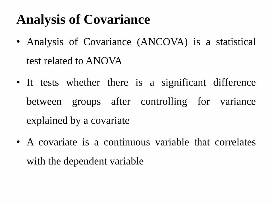
Analysis of Covariance
• Analysis of Covariance (ANCOVA) is a statistical
test related to ANOVA
• It tests whether there is a significant difference
between groups after controlling for variance
explained by a covariate
• A covariate is a continuous variable that correlates
with the dependent variable

Analysis of Covariance
analysis of covariance includes at least one categorical independent
variable and at least one interval or metric independent variable. The
categorical independent variable is called factor, whereas the metric
independent variable is called covariate. The most common use of the
covariate is to remove extraneous variation from the dependent variable,
because the effects of the factors are of major concern. The variation in
the dependent variable due to the covariates is removed by an
adjustment of the dependent variable’s mean value with each treatment
condition.

Variables
1. Dependent variable: Metric data (Continuous)
Ex. Sales, Profit, Market share ,Age, Height etc.
2. Independent variable: Non-metric data(categorical-factor)
Ex. Sales promotion(High, Medium and Low),
Coupon( Rs.20, not Rs. 20)
3. Independent variable: Metric data (Continuous- covariate)
Ex. Number of customers visit in a retail store

Questionnaire
• Metric data: Ex. The sales of this organization is ……,
• Non-metric data: Ex. In-store promotion-
a) High
b) Medium and
c) Low
Ex. Coupon –
(a) Rs.20 discount
(b) No discount
• Metric data: Ex. Number of customers visited in the retail
store.

Covariate
A covariate is a variable that is related to the
Dependent Variable, which you can’t manipulate, but
you want to account for it’s relationship with the
Dependent Variable.

Basic requirements
• Minimum number of Covariate that are uncorrelated
with each other (Why would this be?)
• You want a lot of adjustment with minimum loss of
degrees of freedom
• The change in sums of squares needs to greater than a
change associated with a single degree of freedom lost
for the CV

Basic requirements
Covariates(CV) should also be uncorrelated with the
Independent Variables(IV) (e.g. the Covariate should
be collected before treatment is given) in order to
avoid diminishing the relationship between the
Independent Variables and Dependent Variable(DV).

Applications
• Three major applications
– Increase test sensitivity (main effects and
interactions) by using the CV(s) to account for
more of the error variance therefore making the
error term smaller

Applications…
– Subjects cannot be made equal through random
assignment so CVs are used to adjust scores and
make subjects more similar than without the CV
– This second approach is often used as a way to
improve on poor research designs.
– This should be seen as simple descriptive model
building with no causality

Applications….
– Realize that using CVs can adjust DV scores and
show a larger effect or the CV can eliminate the
effect

Assumptions for ANCOVA
ANOVA assumptions:
• Variance is normally distributed
• Variance is equal between groups
• All measurements are independent
Also, for ANCOVA:
• Relationship between DV and covariate is linear
• The relationship between the DV and covariate is the same for
all groups
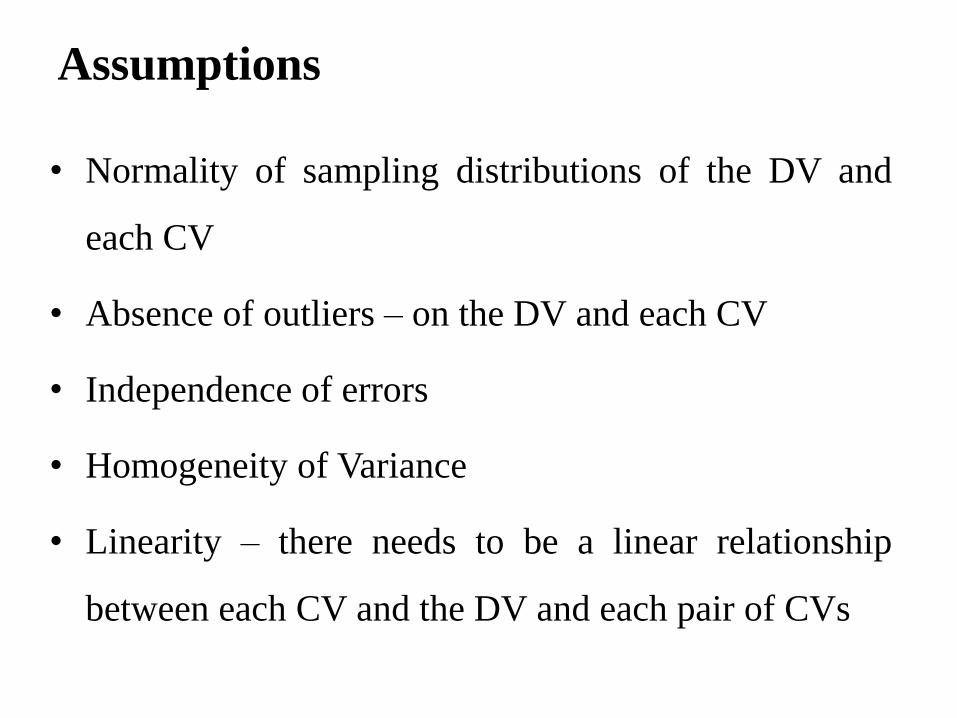
Assumptions
• Normality of sampling distributions of the DV and
each CV
• Absence of outliers – on the DV and each CV
• Independence of errors
• Homogeneity of Variance
• Linearity – there needs to be a linear relationship
between each CV and the DV and each pair of CVs

Assumptions…
• Absence of Multicollinearity –
– Multicollinearity is the presence of high correlations
between the CVs.
– If there are more than one CV and they are highly
correlated they will cancel each other out of the
equations
– How would this work?
– If the correlations nears 1, this is known as singularity
– One of the CVs should be removed

Assumptions…
• Homogeneity of Regression
– The relationship between each CV and the DV should
be the same for each level of the IV

So, what does all that mean?
• This means that you can, in effect, “partial out” a
continuous variable and run an ANOVA on the results
• This is one way that you can run a statistical test with
both categorical and continuous independent
variables

Hypotheses for ANCOVA
• H0 and H1 need to be stated slightly differently for an
ANCOVA than a regular ANOVA
• H0: the group means are equal after controlling for
the covariate
• H1: the group means are not equal after controlling
for the covariate

How does ANCOVA work?
• ANCOVA works by adjusting the total SS, group SS,
and error SS of the independent variable to remove
the influence of the covariate
• However, the sums of squares must also be calculated
for the covariate. For this reason, SSdv will be used
for SS scores for the dependent variable, and SScv will
be used for the covariate.

Examples of Analysis of Covariance
When examining the differences in the mean values of the
dependent variable related to the effect of the controlled
independent variables, it is often necessary to take into account
the influence of uncontrolled independent variables. For
example:
• In determining how different groups exposed to different
commercials evaluate a brand, it may be necessary to control
for prior knowledge.

Examples of Analysis of Covariance..
• In determining how different price levels will affect a
household's cereal consumption, it may be essential to take
household size into account.
• Suppose that we wanted to determine the effect of in-store
promotion and couponing on sales while controlling for the
affect of clientele.

Correlation

Product Moment Correlation
• The product moment correlation, r, summarizes the strength of association
between two metric (interval or ratio scaled) variables, say X and Y.
• It is an index used to determine whether a linear or straight-line relationship
exists between X and Y.
• As it was originally proposed by Karl Pearson, it is also known as the Pearson
correlation coefficient.
• It is also referred to as simple correlation, bivariate correlation, or merely
the correlation coefficient.

Product Moment Correlation
From a sample of n observations, X and Y, the product moment
correlation, r, can be calculated as:

The graph…a Scatter Plot
X
Y
Response variable
(dependent variable)
Explanatory variable
(independent variable)

Scatter Plots of Data with Various Correlation Coefficients
Y
X
Y
X
Y
X
Y
X
Y
X
r = -1 r = -.6 r = 0
r = +.3 r = +1
Y
X r = 0

Y
X
Y
X
Y
Y
X
X
Linear relationships Curvilinear relationships
Linear & Curvilinear Correlation

Y
X
Y
X
Y
Y
X
X
Strong relationships Weak relationships
Linear Correlation

Y
X
Y
X
No relationship

Product Moment Correlation
• r varies between -1.0 and +1.0.
• The correlation coefficient between two variables will be the
same regardless of their underlying units of measurement.

Table-1: Explaining Attitude Toward the City of Residence
Respondent Attitude toward Duration of Importance attached No. the city residence to weather 1 6 10 3 2 9 12 11 3 8 12 4 4 3 4 1 5 10 12 11 6 4 6 1 7 5 8 7 8 2 2 4 9 11 18 8 10 9 9 10 11 10 17 8 12 2 2 5

In this example, suppose a researcher wants to explain attitudes
toward a respondent’s city of residence in terms of duration of
residence in the city. The attitude is measured on 11-point scale
(1= do not like the city, 11= very much like the city), and the
duration of residence is measured in terms of the number of years
the respondents has lived in the city. In addition, importance
attached to the weather is also measured on 11-point scale
(1 = not important, 11 = very important).

Solution:
The correlation coefficient may be calculated as follows:
= (10 + 12 + 12 + 4 + 12 + 6 + 8 + 2 + 18 + 9 + 17 + 2)/12
= 9.333
= (6 + 9 + 8 + 3 + 10 + 4 + 5 + 2 + 11 + 9 + 10 + 2)/12
= 6.583
= (10 -9.33)(6-6.58) + (12-9.33)(9-6.58) + (12-9.33)(8-6.58)
+ (4-9.33)(3-6.58) + (12-9.33)(10-6.58) + (6-9.33)(4-6.58)+ (8-9.33)(5-6.58) +
(2-9.33) (2-6.58) + (18-9.33)(11-6.58) + (9-9.33)(9-6.58) + (17-9.33)(10-6.58) +
(2-9.33) (2-6.58)
= -0.3886 + 6.4614 + 3.7914 + 19.0814 + 9.1314 + 8.5914 + 2.1014 + 33.5714
+ 38.3214 - 0.7986 + 26.2314 + 33.5714
= 179.6668

= (10-9.33)2 + (12-9.33)2 + (12-9.33)2 + (4-9.33)2+ (12-9.33)2 +
(6-9.33)2 + (8-9.33)2 + (2-9.33)2 + (18-9.33)2 + (9-9.33)2 + (17-9.33)2 + (2-9.33)2
= 0.4489 + 7.1289 + 7.1289 + 28.4089 + 7.1289+ 11.0889 +
1.7689 + 53.7289 + 75.1689 + 0.1089 + 58.8289 + 53.7289
= 304.6668
= (6-6.58)2 + (9-6.58)2 + (8-6.58)2 + (3-6.58)2 + (10-6.58)2+ (4-
6.58)2 + (5-6.58)2 + (2-6.58)2 + (11-6.58)2 + (9-6.58)2 + (10-6.58)2 + (2-6.58)2
= 0.3364 + 5.8564 + 2.0164 + 12.8164+ 11.6964 + 6.6564 + 2.4964 +
20.9764 + 19.5364 + 5.8564 + 11.6964 + 20.9764
= 120.9168
Thus,

In this example, r = 0.9361, a value close to 1.0. this means that
respondents’ duration of residence in the city is strongly associated
with their attitude toward the city. Furthermore, the positive sign of r
implies a positive relationship; the longer the duration of residence,
the more favorable the attitude and vice versa.

Decomposition of the Total Variation

• When it is computed for a population rather than a sample, the
product moment correlation is denoted by , the Greek letter
rho. The coefficient r is an estimator of .
• The statistical significance of the relationship between two
variables measured by using r can be conveniently tested. The
hypotheses are:

The test statistics is:
which has a t distribution with (n – 2) degrees of freedom.
For the correlation coefficient calculated based on the
data given in Table.
and the degrees of freedom = 12-2 = 10. From the t distribution
table the critical value of t for a two-tailed test and = 0.05 is
2.228. Hence, the null hypothesis of no relationship between X and
Y is rejected.

Partial Correlation
Partial correlation is used to answer the following questions:
• How strongly are sales related to advertising expenditures when the
effect of price is controlled?
• Is there an association between market share and size of sales force
after adjusting for the effect of sales promotion?
• Are consumers’ perceptions of quality related to their perceptions of
prices when the effect of brand image is controlled?

Partial Correlation
A partial correlation coefficient measures the association between
two variables after controlling for, or adjusting for, the effects of one
or more additional variables.
• Partial correlations have an order associated with them. The order
indicates how many variables are being adjusted or controlled.
• The simple correlation coefficient, r, has a zero-order, as it does not
control for any additional variables while measuring the association
between two variables.

• The coefficient rxy.z is a first-order partial correlation coefficient,
as it controls for the effect of one additional variable, Z.
• A second-order partial correlation coefficient controls for the
effects of two variables, a third-order for the effects of three
variables, and so on.
• The special case when a partial correlation is larger than its
respective zero-order correlation involves a suppressor effect.

Part Correlation Coefficient
The part correlation coefficient represents the correlation between
Y and X when the linear effects of the other independent variables
have been removed from X but not from Y. The part correlation
coefficient, ry(x.z) is calculated as follows:
The partial correlation coefficient is generally viewed as more
important than the part correlation coefficient.

Regression

Regression analysis
Regression analysis examines associative relationships between a
metric dependent variable and one or more independent variables in
the following ways:
• Determine whether the independent variables explain a significant
variation in the dependent variable: whether a relationship exists.
• Determine how much of the variation in the dependent variable can
be explained by the independent variables: strength of the
relationship.

Regression analysis
• Determine the structure or form of the relationship: the
mathematical equation relating the independent and dependent
variables.
• Predict the values of the dependent variable.
• Control for other independent variables when evaluating the
contributions of a specific variable or set of variables.
• Regression analysis is concerned with the nature and degree of
association between variables and does not imply or assume any
causality.

Bivariate regression model
The basic regression equation is
Yi = 0 + i Xi + ei,
where Y = Dependent or criterion variable,
X = Independent or predictor variable,
0 = Intercept of the line,
i = Slope of the line, and
ei = Error term associated with the i th observation.

• Coefficient of determination
The strength of association is
measured by the coefficient of determination, r 2. It varies between
0 and 1 and signifies the proportion of the total variation in Y that is
accounted for by the variation in X.
• Estimated or predicted value
The estimated or predicted value of
Yi is i = a + b x, where i is the predicted value of Yi, and a and b
are estimators of 0 and 1 respectively.

• Regression coefficient
The estimated parameter b is usually
referred to as the non-standardized regression coefficient.
• Scattergram
A scatter diagram, or scattergram, is a plot of the
values of two variables for all the cases or observations.
• Standard error of estimate
This statistic, SEE, is the standard
deviation of the actual Y values from the predicted values.

• Standard error
The standard deviation of b, SEb, is called the
standard error.
• Standardized regression coefficient
Also termed the beta
coefficient or beta weight, this is the slope obtained by the
regression of Y on X when the data are standardized.

• Sum of squared errors
The distances of all the points from the
regression line are squared and added together to arrive at the sum
of squared errors, which is a measure of total error,
• t statistic
A t statistic with n - 2 degrees of freedom can be used to
test the null hypothesis that no linear relationship exists between X
and Y, or H0: β = 0, where t=b /SEb
e j S 2

Conducting Bivariate Regression Analysis
A scatter diagram, or scattergram, is a plot of the values of
two variables for all the cases or observations.
The most commonly used technique for fitting a straight
line to a scattergram is the least-squares procedure. In fitting the
line, the least-squares procedure minimizes the sum of squared
errors, . e j S 2

Conducting Bivariate Regression Analysis
Plot the Scatter Diagram
Formulate the General Model
Estimate the Parameters
Estimate Standardized Regression Coefficients
Test for Significance
Determine the Strength and Significance of Association
Check Prediction Accuracy
Examine the Residuals
Cross-Validate the Model

Plot of Attitude with Duration
4.5 2.25 6.75 11.25 9 13.5
9
3
6
15.75 18
Duration of Residence
Att
itu
de

Which Straight Line Is Best?
9
6
3
2.25 4.5 6.75 9 11.25 13.5 15.75 18
Line 1
Line 2
Line 3
Line 4

Bivariate Regression
X2 X1 X3 X5 X4
YJ
eJ
eJ
YJ
X
Y β0 + β1X

Formulate the Bivariate Regression Model
In the bivariate regression model, the general form of a straight line is:
where
Y = Dependent or criterion variable
X = Independent or predictor variable
= Intercept of the line
= Slop of the line
The regression procedure adds an error term to account for the
probabilistic or stochastic nature of the relationship. The basic regression
equation becomes:
Where is the error term associated with the ith observation.

Estimate the Parameters
In most cases, and are unknown and are estimated from the
sample observations using the equation
Where is the estimated or predicted value of and a and b are
estimators of and , respectively.
The slop, b, may be computed in terms of the covariance between X
and Y,( ), and the variance of X as:

The intercept, a, may then calculated using:

The estimation of parameters may be illustrated as follows:
= 10X6 + 12X9 + 12X8 + 4X3 + 12X10 + 6X4 +
8X5 + 2X2 + 18X11 + 9X9 + 17X10+ 2X2
= 917
= 1,350
It may be recalled from earlier calculations of the simple correlation
that

Given n = 12, b can be calculated as:

Estimate the Standardized Regression Coefficient
• Standardization is the process by which the raw data are transformed into
new variables that have a mean of 0 and a variance of 1.
• When the data are standardized, the intercept assumes a value of 0.
• The term beta coefficient or beta weight is used to denote the
standardized regression coefficient.
Byx = Bxy = rxy
• There is a simple relationship between the standardized and non-
standardized regression coefficients:
Byx = byx (Sx /Sy)

Test for Significance
The statistical significance of the linear relationship between X and
Y may be tested by examining the hypotheses:
A t- statistic with n - 2 degrees of freedom can be used,
where
SEb denotes the standard deviation of b and is called the standard
error.

Test for Significance
Using a computer program, the regression of attitude on duration of
residence, using the data shown in Table-1, yielded the results shown in
Table -2. The intercept, a, equals 1.0793, and the slope, b, equals 0.5897.
Therefore, the estimated equation is:
Attitude ( ) = 1.0793 + 0.5897 (Duration of residence)
The standard error, or standard deviation of b is estimated as 0.07008, and
the value of the t statistic as t = 0.5897/0.0700 = 8.414, with n - 2 = 10
degrees of freedom.
From Table in the Statistical Appendix, we see that the critical value of t
with 10 degrees of freedom and = 0.05 is 2.228 for a two-tailed test.
Since the calculated value of t is larger than the critical value, the null
hypothesis is rejected.

Determine the Strength and Significance of Association
The total variation, SSy, may be decomposed into the variation
accounted for by the regression line, SSreg, and the error or residual
variation, SSerror or SSres, as follows:
SSy = SSreg + SSres
Where

Decomposition of the Total Variation in Bivariate Regression
X2 X1 X3 X5 X4 X
Residual Variation
SSres Explained Variation
SSreg
Y

Determine the Strength and Significance of Association
The strength of association may then be calculated as follows:
To illustrate the calculations of r2, let us consider again the effect of
attitude toward the city on the duration of residence. It may be
recalled from earlier calculations of the simple correlation
coefficient that:
= 120.9168

Determine the Strength and Significance of Association
The predicted values ( ) can be calculated using the regression
equation:
Attitude ( ) = 1.0793 + 0.5897 (Duration of residence)
For the first observation in Table -1, this value is:
( ) = 1.0793 + 0.5897 x 10 = 6.9763.
For each successive observation, the predicted values are, in order,
8.1557, 8.1557, 3.4381, 8.1557, 4.6175, 5.7969, 2.2587, 11.6939,
6.3866, 11.1042, and 2.2587.
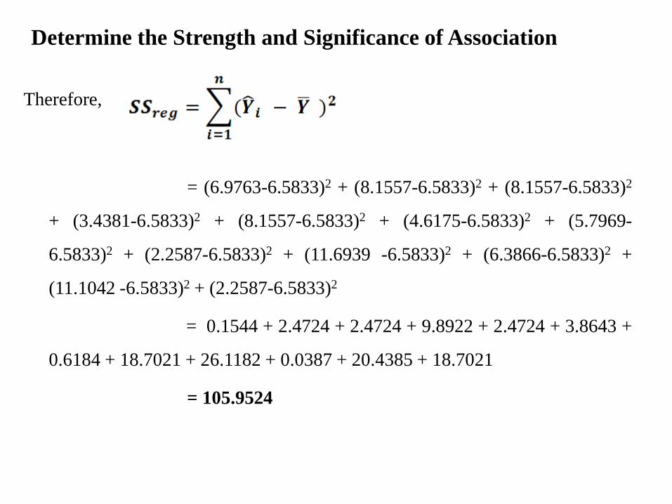
Determine the Strength and Significance of Association
Therefore,
= (6.9763-6.5833)2 + (8.1557-6.5833)2 + (8.1557-6.5833)2
+ (3.4381-6.5833)2 + (8.1557-6.5833)2 + (4.6175-6.5833)2 + (5.7969-
6.5833)2 + (2.2587-6.5833)2 + (11.6939 -6.5833)2 + (6.3866-6.5833)2 +
(11.1042 -6.5833)2 + (2.2587-6.5833)2
= 0.1544 + 2.4724 + 2.4724 + 9.8922 + 2.4724 + 3.8643 +
0.6184 + 18.7021 + 26.1182 + 0.0387 + 20.4385 + 18.7021
= 105.9524
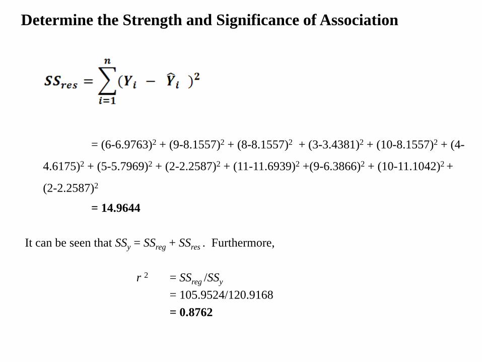
Determine the Strength and Significance of Association
= (6-6.9763)2 + (9-8.1557)2 + (8-8.1557)2 + (3-3.4381)2 + (10-8.1557)2 + (4-
4.6175)2 + (5-5.7969)2 + (2-2.2587)2 + (11-11.6939)2 +(9-6.3866)2 + (10-11.1042)2 +
(2-2.2587)2
= 14.9644
It can be seen that SSy = SSreg + SSres . Furthermore,
r 2 = SSreg /SSy
= 105.9524/120.9168
= 0.8762

Determine the Strength and Significance of Association
Another, equivalent test for examining the significance of the
linear relationship between X and Y (significance of b) is the test for the
significance of the coefficient of determination. The hypothesis in this
case are:
H0: R2
pop = 0
H1: R2
pop > 0

Determine the Strength and Significance of Association
The appropriate test statistic is the F statistic:
which has an F distribution with 1 and n - 2 degrees of freedom. The F test is a
generalized form of the t test (see Chapter 15). If a random variable is t distributed
with n degrees of freedom, then t2 is F distributed with 1 and n degrees of freedom.
Hence, the F test for testing the significance of the coefficient of determination is
equivalent to testing the following hypotheses:
or
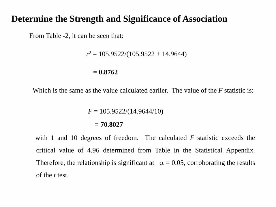
Determine the Strength and Significance of Association
From Table -2, it can be seen that:
r2 = 105.9522/(105.9522 + 14.9644)
= 0.8762
Which is the same as the value calculated earlier. The value of the F statistic is:
F = 105.9522/(14.9644/10)
= 70.8027
with 1 and 10 degrees of freedom. The calculated F statistic exceeds the
critical value of 4.96 determined from Table in the Statistical Appendix.
Therefore, the relationship is significant at = 0.05, corroborating the results
of the t test.

Bivariate Regression
Multiple R 0.93608
R2 0.87624
Adjusted R2 0.86387
Standard Error 1.22329
ANALYSIS OF VARIANCE
df Sum of Squares Mean Square
Regression 1 105.95222 105.95222
Residual 10 14.96444 1.49644
F = 70.80266 Significance of F = 0.0000
VARIABLES IN THE EQUATION
Variable b SEb Beta (ß) T Sign. of T
Duration 0.58972 0.07008 0.93608 8.414 0.0000
(Constant) 1.07932 0.74335 1.452 0.1772

Check Prediction Accuracy
To estimate the accuracy of predicted values, , it is useful to calculate the standard
error of estimate, SEE.
or
or more generally, if there are k independent variables,
For the data given in Table -2, the SEE is estimated as follows:
= 1.22329

Assumptions
• The error term is normally distributed. For each fixed value of X, the
distribution of Y is normal.
• The means of all these normal distributions of Y, given X, lie on a straight
line with slope b.
• The mean of the error term is 0.
• The variance of the error term is constant. This variance does not depend on
the values assumed by X.
• The error terms are uncorrelated. In other words, the observations have been
drawn independently.

Multiple Regression

Multiple Regression
The general form of the multiple regression model is as follows:
which is estimated by the following equation:
As before, the coefficient a represents the intercept, but the b's
are now the partial regression coefficients.

Statistics Associated with Multiple Regression
• Adjusted R2
R2, coefficient of multiple determination, is adjusted for the
number of independent variables and the sample size to account for the
diminishing returns. After the first few variables, the additional independent
variables do not make much contribution.
• Coefficient of multiple determination
The strength of association in multiple
regression is measured by the square of the multiple correlation coefficient,
R2, which is also called the coefficient of multiple determination.

• F test : The F test is used to test the null hypothesis that the coefficient of
multiple determination in the population, R2pop, is zero. This is equivalent
to testing the null hypothesis. The test statistic has an F distribution with k
and (n - k - 1) degrees of freedom.
• Partial F test :The significance of a partial regression coefficient, , of
Xi may be tested using an incremental F statistic. The incremental F
statistic is based on the increment in the explained sum of squares resulting
from the addition of the independent variable Xi to the regression equation
after all the other independent variables have been included.
• Partial regression coefficient: The partial regression coefficient, b1,
denotes the change in the predicted value, , per unit change in X1 when
the other independent variables, X2 to Xk , are held constant.

Partial Regression Coefficients
To understand the meaning of a partial regression
coefficient, let us consider a case in which there are two
independent variables, so that:
First, note that the relative magnitude of the partial
regression coefficient of an independent variable is, in general,
different from that of its bivariate regression coefficient.

• The interpretation of the partial regression coefficient, b1, is
that it represents the expected change in Y when X1 is changed by
one unit but X2 is held constant or otherwise controlled. Likewise,
b2 represents the expected change in Y for a unit change in X2, when
X1 is held constant. Thus, calling b1 and b2 partial regression
coefficients is appropriate.
• It can also be seen that the combined effects of X1 and X2 on
Y are additive. In other words, if X1 and X2 are each changed by one
unit, the expected change in Y would be (b1+b2).

• Suppose one was to remove the effect of X2 from X1. This could be
done by running a regression of X1 on X2. In other words, one
would estimate the equation = a + b X2 and calculate the
residual Xr = (X1 - ). The partial regression coefficient, b1, is
then equal to the bivariate regression coefficient, br , obtained from
the equation = a + br Xr .

Partial Regression Coefficients
• Extension to the case of k variables is straightforward. The partial regression coefficient,
b1, represents the expected change in Y when X1 is changed by one unit and X2 through Xk
are held constant. It can also be interpreted as the bivariate regression coefficient, b, for
the regression of Y on the residuals of X1, when the effect of X2 through Xk has been
removed from X1.
• The relationship of the standardized to the non-standardized coefficients remains the
same as before:
The estimated regression equation is:
( ) = 0.33732 + 0.48108 X1 + 0.28865 X2
or
Attitude = 0.33732 + 0.48108 (Duration) + 0.28865 (Importance)

Multiple Regression
Multiple R 0.97210
R2 0.94498
Adjusted R2 0.93276
Standard Error 0.85974
ANALYSIS OF VARIANCE
df Sum of Squares Mean Square
Regression 2 114.26425 57.13213
Residual 9 6.65241 0.73916
F = 77.29364 Significance of F = 0.0000
VARIABLES IN THE EQUATION
Variable b SEb Beta (ß) T Significance
of T
IMPORTANCE 0.28865 0.08608 0.31382 3.353 0.0085
DURATION 0.48108 0.05895 0.76363 8.160 0.0000
(Constant) 0.33732 0.56736 0.595 0.5668

Determine the Strength of Association
The total variation, SSy, may be decomposed into the variation
accounted for by the regression line, SSreg, and the error or residual
variation, SSerror or SSres, as follows:
SSy = SSreg + SSres
Where

• The strength of association is measured by the square of the multiple
correlation coefficient, R2, which is also called the coefficient of
multiple determination.
• R2 is adjusted for the number of independent variables and the
sample size by using the following formula:

This is equivalent to the following null hypothesis:
The overall test can be conducted by using an F statistic:
which has an F distribution with k and (n - k -1) degrees of freedom.
Significance testing

• Testing for the significance of the can be done in a manner
similar to that in the bivariate case by using t tests. The
significance of the partial coefficient for importance attached to
weather may be tested by the following equation:
• which has a t distribution with n - k -1 degrees of freedom.
Significance testing

Examination of Residuals
• A residual is the difference between the observed value of Yi and the value
predicted by the regression equation .
• Scattergrams of the residuals, in which the residuals are plotted against the
predicted values, , time, or predictor variables, provide useful insights in
examining the appropriateness of the underlying assumptions and regression
model fit.
• The assumption of a normally distributed error term can be examined by
constructing a histogram of the residuals.
• The assumption of constant variance of the error term can be examined by
plotting the residuals against the predicted values of the dependent variable,
Examination of Residuals
• A plot of residuals against time, or the sequence of observations, will
throw some light on the assumption that the error terms are uncorrelated.
• Plotting the residuals against the independent variables provides evidence
of the appropriateness or inappropriateness of using a linear model. Again,
the plot should result in a random pattern.
• To examine whether any additional variables should be included in the
regression equation, one could run a regression of the residuals on the
proposed variables.
• If an examination of the residuals indicates that the assumptions
underlying linear regression are not met, the researcher can transform the
variables in an attempt to satisfy the assumptions.

Multicollinearity
• Multicollinearity arises when intercorrelations among the predictors are
very high.
Multicollinearity can result in several problems, including:
• The partial regression coefficients may not be estimated precisely.
The standard errors are likely to be high.
• The magnitudes, as well as the signs of the partial regression
coefficients, may change from sample to sample.
• It becomes difficult to assess the relative importance of the
independent variables in explaining the variation in the dependent
variable.
• Predictor variables may be incorrectly included or removed in
stepwise regression.

Multicollinearity
• A simple procedure for adjusting for multicollinearity consists of using only
one of the variables in a highly correlated set of variables.
• Alternatively, the set of independent variables can be transformed into a new
set of predictors that are mutually independent by using techniques such as
principal components analysis.
• More specialized techniques, such as ridge regression and latent root
regression, can also be used.
Regression with Dummy Variables
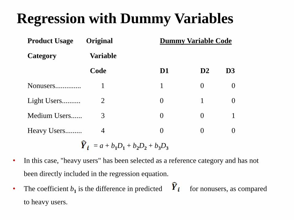
Product Usage Original Dummy Variable Code
Category Variable
Code D1 D2 D3
Nonusers.............. 1 1 0 0
Light Users.......... 2 0 1 0
Medium Users...... 3 0 0 1
Heavy Users......... 4 0 0 0
= a + b1D1 + b2D2 + b3D3
• In this case, "heavy users" has been selected as a reference category and has not
been directly included in the regression equation.
• The coefficient b1 is the difference in predicted for nonusers, as compared
to heavy users.

Analysis of Variance and Covariance with Regression
Product Usage Predicted Mean
Category Value Value
In regression with dummy variables, the predicted for each category is the
mean of Y for each category.
Nonusers............... a + b1 a + b1
Light Users........... a + b2 a + b2
Medium Users....... a + b3 a + b3
Heavy Users.......... a a

Analysis of Variance and Covariance with Regression
Given this equivalence, it is easy to see further relationships between dummy
variable regression and one-way ANOVA.
Dummy Variable Regression One-Way ANOVA

Discriminant Analysis
Discriminant Analysis
Discriminant analysis is a technique for
analyzing data when the criterion or dependent variable
is categorical and the predictor or independent
variables are interval in nature.

The objectives of discriminant analysis
• Development of discriminant functions, or linear combinations of
the predictor or independent variables, which will best discriminate
between the categories of the criterion or dependent variable
(groups).
• Examination of whether significant differences exist among the
groups, in terms of the predictor variables.
• Determination of which predictor variables contribute to most of the
intergroup differences.

The objectives….
• Classification of cases to one of the groups based on the values of
the predictor variables.
• Evaluation of the accuracy of classification.
• When the criterion variable has two categories, the technique is
known as two-group discriminant analysis.
• When three or more categories are involved, the technique is
referred to as multiple discriminant analysis.

The objectives….
• The main distinction is that, in the two-group case, it is possible to
derive only one discriminant function. In multiple discriminant
analysis, more than one function may be computed. In general, with
G groups and k predictors, it is possible to estimate up to the smaller
of G - 1, or k, discriminant functions.
• The first function has the highest ratio of between-groups to within-
groups sum of squares. The second function, uncorrelated with the
first, has the second highest ratio, and so on. However, not all the
functions may be statistically significant.

Geometric Interpretation
X 2
X 1
G1
G2
D
G1 G2
2 2 2 2 2 2 2 2 2 2
2 1 1
1 1
2 2 2 2 1
1 1 1 1 1 1 1 1 1

Discriminant Analysis Model
The discriminant analysis model involves linear combinations of the following form:
D = b0 + b1X1 + b2X2 + b3X3 + . . . + bkXk
Where:
D = Discriminant score
b 's = Discriminant coefficient or weight
X 's = Predictor or independent variable
• The coefficients, or weights (b), are estimated so that the groups differ as much as
possible on the values of the discriminant function.
• This occurs when the ratio of between-group sum of squares to within-group sum of
squares for the discriminant scores is at a maximum.

Statistics Associated with Discriminant Analysis
• Canonical correlation
Canonical correlation measures the extent
of association between the discriminant scores and the groups. It is a
measure of association between the single discriminant function and
the set of dummy variables that define the group membership.
• Centroid
The centroid is the mean values for the discriminant scores
for a particular group. There are as many centroids as there are
groups, as there is one for each group. The means for a group on all
the functions are the group centroids.

• Classification matrix
Sometimes also called confusion or
prediction matrix, the classification matrix contains the number of
correctly classified and misclassified cases.
• Discriminant function coefficients
The discriminant function
coefficients (unstandardized) are the multipliers of variables, when
the variables are in the original units of measurement.

• Discriminant scores
The unstandardized coefficients are multiplied
by the values of the variables. These products are summed and
added to the constant term to obtain the discriminant scores.
• Eigenvalue
For each discriminant function, the Eigenvalue is the
ratio of between-group to within-group sums of squares. Large
Eigenvalues imply superior functions.

• F values and their significance
These are calculated from a one-
way ANOVA, with the grouping variable serving as the categorical
independent variable. Each predictor, in turn, serves as the metric
dependent variable in the ANOVA.
• Group means and group standard deviations
These are computed
for each predictor for each group.

• Pooled within-group correlation matrix
The pooled within-group
correlation matrix is computed by averaging the separate covariance
matrices for all the groups.
• Standardized discriminant function coefficients
The standardized
discriminant function coefficients are the discriminant function
coefficients and are used as the multipliers when the variables have
been standardized to a mean of 0 and a variance of 1.

• Structure correlations: Also referred to as discriminant loadings, the
structure correlations represent the simple correlations between the
predictors and the discriminant function.
• Total correlation matrix: If the cases are treated as if they were from a
single sample and the correlations computed, a total correlation matrix is
obtained.
• Wilks' : Sometimes also called the U statistic, Wilks' for each
predictor is the ratio of the within-group sum of squares to the total sum of
squares. Its value varies between 0 and 1. Large values
of (near 1) indicate that group means do not seem to be different. Small
values of (near 0) indicate that the group means seem to be different.

Conducting Discriminant Analysis
Assess Validity of Discriminant Analysis
Estimate the Discriminant Function Coefficients
Determine the Significance of the Discriminant Function
Formulate the Problem
Interpret the Results

Formulate the Problem
• Identify the objectives, the criterion variable, and the independent
variables.
• The criterion variable must consist of two or more mutually exclusive
and collectively exhaustive categories.
• The predictor variables should be selected based on a theoretical model
or previous research, or the experience of the researcher.

Formulate the Problem…
• One part of the sample, called the estimation or analysis sample, is
used for estimation of the discriminant function.
• The other part, called the holdout or validation sample, is reserved
for validating the discriminant function.
• Often the distribution of the number of cases in the analysis and
validation samples follows the distribution in the total sample.

Information on Resort Visits: Analysis Sample
Annual Attitude Importance Household Age of Amount
Resort Family Toward Attached Size Head of Spent on
No. Visit Income Travel to Family Household Family
($000) Vacation Vacation
1 1 50.2 5 8 3 43 M (2)
2 1 70.3 6 7 4 61 H (3)
3 1 62.9 7 5 6 52 H (3)
4 1 48.5 7 5 5 36 L (1)
5 1 52.7 6 6 4 55 H (3)
6 1 75.0 8 7 5 68 H (3)
7 1 46.2 5 3 3 62 M (2)
8 1 57.0 2 4 6 51 M (2)
9 1 64.1 7 5 4 57 H (3)
10 1 68.1 7 6 5 45 H (3)
11 1 73.4 6 7 5 44 H (3)
12 1 71.9 5 8 4 64 H (3)
13 1 56.2 1 8 6 54 M (2)
14 1 49.3 4 2 3 56 H (3)
15 1 62.0 5 6 2 58 H (3)

Information on Resort Visits….
Annual Attitude Importance Household Age of Amount
Resort Family Toward Attached Size Head of Spent on No. Visit Income Travel to Family Household Family
($000) Vacation Vacation
16 2 32.1 5 4 3 58 L (1)
17 2 36.2 4 3 2 55 L (1)
18 2 43.2 2 5 2 57 M (2)
19 2 50.4 5 2 4 37 M (2)
20 2 44.1 6 6 3 42 M (2)
21 2 38.3 6 6 2 45 L (1)
22 2 55.0 1 2 2 57 M (2)
23 2 46.1 3 5 3 51 L (1)
24 2 35.0 6 4 5 64 L (1)
25 2 37.3 2 7 4 54 L (1)
26 2 41.8 5 1 3 56 M (2)
27 2 57.0 8 3 2 36 M (2)
28 2 33.4 6 8 2 50 L (1)
29 2 37.5 3 2 3 48 L (1)
30 2 41.3 3 3 2 42 L (1)

Information on Resort Visits: Holdout Sample
Annual Attitude Importance Household Age of Amount
Resort Family Toward Attached Size Head of Spent on No. Visit Income Travel to Family Household Family
($000) Vacation Vacation
1 1 50.8 4 7 3 45 M(2)
2 1 63.6 7 4 7 55 H (3)
3 1 54.0 6 7 4 58 M(2)
4 1 45.0 5 4 3 60 M(2)
5 1 68.0 6 6 6 46 H (3)
6 1 62.1 5 6 3 56 H (3)
7 2 35.0 4 3 4 54 L (1)
8 2 49.6 5 3 5 39 L (1)
9 2 39.4 6 5 3 44 H (3)
10 2 37.0 2 6 5 51 L (1)
11 2 54.5 7 3 3 37 M(2)
12 2 38.2 2 2 3 49 L (1)

Conducting Discriminant Analysis :Estimate the
Discriminant Function Coefficients
• The direct method involves estimating the discriminant
function so that all the predictors are included
simultaneously.
• In stepwise discriminant analysis, the predictor
variables are entered sequentially, based on their ability
to discriminate among groups.

Results of Two-Group Discriminant Analysis GROUP MEANS VISIT INCOME TRAVEL VACATION HSIZE AGE 1 60.52000 5.40000 5.80000 4.33333 53.73333 2 41.91333 4.33333 4.06667 2.80000 50.13333 Total 51.21667 4.86667 4.9333 3.56667 51.93333 Group Standard Deviations 1 9.83065 1.91982 1.82052 1.23443 8.77062 2 7.55115 1.95180 2.05171 .94112 8.27101 Total 12.79523 1.97804 2.09981 1.33089 8.57395 Pooled Within-Groups Correlation Matrix INCOME TRAVEL VACATION HSIZE AGE INCOME 1.00000 TRAVEL 0.19745 1.00000 VACATION 0.09148 0.08434 1.00000 HSIZE 0.08887 -0.01681 0.07046 1.00000 AGE - 0.01431 -0.19709 0.01742 -0.04301 1.00000 Wilks' (U-statistic) and univariate F ratio with 1 and 28 degrees of freedom Variable Wilks' F Significance INCOME 0.45310 33.800 0.0000 TRAVEL 0.92479 2.277 0.1425 VACATION 0.82377 5.990 0.0209 HSIZE 0.65672 14.640 0.0007 AGE 0.95441 1.338 0.2572 Cont.

Results of Two-Group Discriminant Analysis
CANONICAL DISCRIMINANT FUNCTIONS % of Cum Canonical After Wilks' Function Eigenvalue Variance % Correlation Function Chi-square df Significance : 0 0 .3589 26.130 5 0.0001 1* 1.7862 100.00 100.00 0.8007 : * marks the 1 canonical discriminant functions remaining in the analysis. Standard Canonical Discriminant Function Coefficients FUNC 1 INCOME 0.74301 TRAVEL 0.09611 VACATION 0.23329 HSIZE 0.46911 AGE 0.20922 Structure Matrix: Pooled within-groups correlations between discriminating variables & canonical discriminant functions (variables ordered by size of correlation within function) FUNC 1 INCOME 0.82202 HSIZE 0.54096 VACATION 0.34607 TRAVEL 0.21337 AGE 0.16354 Cont.

Cont.
Results of Two-Group Discriminant Analysis
Unstandardized Canonical Discriminant Function Coefficients
FUNC 1
INCOME 0.8476710E-01
TRAVEL 0.4964455E-01
VACATION 0.1202813
HSIZE 0.4273893
AGE 0.2454380E-01
(constant) -7.975476
Canonical discriminant functions evaluated at group means (group centroids)
Group FUNC 1
1 1.29118
2 -1.29118
Classification results for cases selected for use in analysis
Predicted Group Membership
Actual Group No. of Cases 1 2
Group 1 15 12 3
80.0% 20.0%
Group 2 15 0 15
0.0% 100.0%
Percent of grouped cases correctly classified: 90.00%

Results of Two-Group Discriminant Analysis
Classification Results for cases not selected for use in the analysis (holdout sample) Predicted Group Membership Actual Group No. of Cases 1 2 Group 1 6 4 2 66.7% 33.3% Group 2 6 0 6 0.0% 100.0% Percent of grouped cases correctly classified: 83.33%.

Determine the Significance of Discriminant Function
• The null hypothesis that, in the population, the means of all discriminant
functions in all groups are equal can be statistically tested.
• In SPSS this test is based on Wilks' . If several functions are tested
simultaneously (as in the case of multiple discriminant analysis), the
Wilks' statistic is the product of the univariate for each function. The
significance level is estimated based on a chi-square transformation of
the statistic.
• If the null hypothesis is rejected, indicating significant discrimination,
one can proceed to interpret the results.

Interpret the Results
• The interpretation of the discriminant weights, or coefficients, is
similar to that in multiple regression analysis.
• Given the multicollinearity in the predictor variables, there is no
unambiguous measure of the relative importance of the predictors
in discriminating between the groups.
• With this caveat in mind, we can obtain some idea of the relative
importance of the variables by examining the absolute magnitude
of the standardized discriminant function coefficients.

Interpret the Results
• Some idea of the relative importance of the predictors can also be
obtained by examining the structure correlations, also called
canonical loadings or discriminant loadings. These simple
correlations between each predictor and the discriminant function
represent the variance that the predictor shares with the function.
• Another aid to interpreting discriminant analysis results is to
develop a Characteristic profile for each group by describing each
group in terms of the group means for the predictor variables.

Assess Validity of Discriminant Analysis
• Many computer programs, such as SPSS, offer a leave-one-out cross-validation
option.
• The discriminant weights, estimated by using the analysis sample, are multiplied by
the values of the predictor variables in the holdout sample to generate discriminant
scores for the cases in the holdout sample. The cases are then assigned to groups
based on their discriminant scores and an appropriate decision rule. The hit ratio, or
the percentage of cases correctly classified, can then be determined by summing the
diagonal elements and dividing by the total number of cases.
• It is helpful to compare the percentage of cases correctly classified by discriminant
analysis to the percentage that would be obtained by chance. Classification accuracy
achieved by discriminant analysis should be at least 25% greater than that obtained by
chance.

Results of Three-Group Discriminant Analysis
Group Means
AMOUNT INCOME TRAVEL VACATION HSIZE AGE
1 38.57000 4.50000 4.70000 3.10000 50.30000
2 50.11000 4.00000 4.20000 3.40000 49.50000
3 64.97000 6.10000 5.90000 4.20000 56.00000
Total 51.21667 4.86667 4.93333 3.56667 51.93333
Group Standard Deviations
1 5.29718 1.71594 1.88856 1.19722 8.09732
2 6.00231 2.35702 2.48551 1.50555 9.25263
3 8.61434 1.19722 1.66333 1.13529 7.60117
Total 12.79523 1.97804 2.09981 1.33089 8.57395
Pooled Within-Groups Correlation Matrix
INCOME TRAVEL VACATION HSIZE AGE
INCOME 1.00000
TRAVEL 0.05120 1.00000
VACATION 0.30681 0.03588 1.00000
HSIZE 0.38050 0.00474 0.22080 1.00000
AGE -0.20939 -0.34022 -0.01326 -0.02512 1.00000 Cont.

Results of Three-Group Discriminant Analysis
Wilks' (U-statistic) and univariate F ratio with 2 and 27 degrees of freedom. Variable Wilks' Lambda F Significance INCOME 0.26215 38.00 0.0000 TRAVEL 0.78790 3.634 0.0400 VACATION 0.88060 1.830 0.1797 HSIZE 0.87411 1.944 0.1626 AGE 0.88214 1.804 0.1840
CANONICAL DISCRIMINANT FUNCTIONS % of Cum Canonical After Wilks' Function Eigenvalue Variance % Correlation Function Chi-square df Signifi. : 0 0.1664 44.831 10 0.00 1* 3.8190 93.93 93.93 0.8902 : 1 0.8020 5.517 4 0.24 2* 0.2469 6.07 100.00 0.4450 : * marks the two canonical discriminant functions remaining in the analysis.
Standardized Canonical Discriminant Function Coefficients FUNC 1 FUNC 2 INCOME 1.04740 -0.42076 TRAVEL 0.33991 0.76851 VACATION -0.14198 0.53354 HSIZE -0.16317 0.12932 AGE 0.49474 0.52447 Cont.

Results of Three-Group Discriminant Analysis
Structure Matrix:
Pooled within-groups correlations between discriminating variables and canonical discriminant
functions (variables ordered by size of correlation within function)
FUNC 1 FUNC 2
INCOME 0.85556* -0.27833
HSIZE 0.19319* 0.07749
VACATION 0.21935 0.58829*
TRAVEL 0.14899 0.45362*
AGE 0.16576 0.34079*
Unstandardized canonical discriminant function coefficients FUNC 1 FUNC 2
INCOME 0.1542658 -0.6197148E-01
TRAVEL 0.1867977 0.4223430
VACATION -0.6952264E-01 0.2612652
HSIZE -0.1265334 0.1002796
AGE 0.5928055E-01 0.6284206E-01
(constant) -11.09442 -3.791600
Canonical discriminant functions evaluated at group means (group centroids) Group FUNC 1 FUNC 2
1 -2.04100 0.41847
2 -0.40479 -0.65867
3 2.44578 0.24020 Cont.

Results of Three-Group Discriminant Analysis
Classification Results: Predicted Group Membership Actual Group No. of Cases 1 2 3 Group 1 10 9 1 0 90.0% 10.0% 0.0% Group 2 10 1 9 0 10.0% 90.0% 0.0% Group 3 10 0 2 8 0.0% 20.0% 80.0% Percent of grouped cases correctly classified: 86.67%
Classification results for cases not selected for use in the analysis Predicted Group Membership Actual Group No. of Cases 1 2 3 Group 1 4 3 1 0 75.0% 25.0% 0.0% Group 2 4 0 3 1 0.0% 75.0% 25.0% Group 3 4 1 0 3 25.0% 0.0% 75.0% Percent of grouped cases correctly classified: 75.00%

All-Groups Scattergram
-4.0
Across: Function 1 Down: Function 2
4.0
0.0
-6.0 4.0 0.0 -2.0 -4.0 2.0 6.0
1 1
1 1
1
1
1
1
1
2 1 2
2 2
2
2 3 3 3 3
3
3 3
2
3
*
*
*
* indicates a group
centroid

Territorial Map
-4.0
Across: Function 1 Down: Function 2
4.0
0.0
-6.0 4.0 0.0 -2.0 -4.0 2.0 6.0
1
1 3
*
-8.0
-8.0
8.0
8.0
1 3
1 3
1 3
1 3 1 3
1 3 1 3
1 1 2 3 1 1 2 2 3 3
1 1 2 2 1 1 1 2 2 2 2 3 3
1 1 1 2 2
1 1 2 2
1 1 2 2
1 1 1 2 2
1 1 2 2
1 1 2 2
1 1 1 2 2 1 1 1 2 2
1 1 2 2 2
2 2 3 2 3 3
2 2 3 3
2 2 3
2 2 3
2 2 3
2 2 3 3
2 3 3
2 3 3
2 3 3
* *
* Indicates a
group centroid

Stepwise Discriminant Analysis
• Stepwise discriminant analysis is analogous to stepwise multiple regression in
that the predictors are entered sequentially based on their ability to
discriminate between the groups.
• An F ratio is calculated for each predictor by conducting a univariate analysis
of variance in which the groups are treated as the categorical variable and the
predictor as the criterion variable.
• The predictor with the highest F ratio is the first to be selected for inclusion in
the discriminant function, if it meets certain significance and tolerance
criteria.
• A second predictor is added based on the highest adjusted or partial F ratio,
taking into account the predictor already selected.

Stepwise Discriminant Analysis
• Each predictor selected is tested for retention based on its association with
other predictors selected.
• The process of selection and retention is continued until all predictors meeting
the significance criteria for inclusion and retention have been entered in the
discriminant function.
• The selection of the stepwise procedure is based on the optimizing criterion
adopted. The Mahalanobis procedure is based on maximizing a generalized
measure of the distance between the two closest groups.
• The order in which the variables were selected also indicates their importance
in discriminating between the groups.

The Logit Model

The Logit Model
• The dependent variable is binary and there are several
independent variables that are metric
• The binary logit model commonly deals with the issue of
how likely is an observation to belong to each group
• It estimates the probability of an observation belonging to a
particular group

Conducting Binary Logit analysis
Formulate the Binary Logit problem
Estimate the Binary Logit problem
Determine Model fit
Test the significance of individual parameter
Interpret the coefficient

Binary Logit Model Formulation
The probability of success may be modeled using the logit model as:
or

Model Formulation
Where

Properties of the Logit Model
• Although Xi may vary from - to + , P is constrained to
lie between 0 and 1.
• When Xi approaches - , P approaches 0.
• When Xi approaches + , P approaches 1.
• When OLS regression is used, P is not constrained to lie
between 0 and 1.

Estimation and Model Fit
• The estimation procedure is called the maximum likelihood method.
• Fit: Cox & Snell R Square and Nagelkerke R Square.
• Both these measures are similar to R2 in multiple regression.
• The Cox & Snell R Square can not equal 1.0, even if the fit is perfect.
• This limitation is overcome by the Nagelkerke R Square.
• Compare predicted and actual values of Y to determine the percentage of
correct predictions.

Significance Testing
The significance of the estimated coefficients is based on Wald’s
statistic.
Where,
ai = Logistical coefficient for that predictor variable
SEai = Standard error of the logistical coefficient
The Wald statistic is chi-square distributed with 1 degree of
freedom if the variable is metric and the number of categories minus
1 if the variable is nonmetric.

Interpretation of Coefficients
• If Xi is increased by one unit, the log odds will change by ai units,
when the effect of other independent variables is held constant.
• The sign of ai will determine whether the probability increases (if
the sign is positive) or decreases (if the sign is negative) by this
amount.

Example-1
We illustrate the logit model by analyzing the data of table. This
table gives the data for 30 respondents, 15 of whom are brand
loyal(indicate by 1) and 15 of whom are not (indicated by 0). We
also measure attitude toward the brand ( Brand), attitude toward the
product category(Product), and attitude toward shopping (S
hopping), all on a 1 (unfavorable) to 7 (favorable) scale. The
objective is to estimate the loyalty of consumer being brand loyal as
a function of attitude toward the brand, the product category, and
shopping.

Explaining Brand Loyalty ….
No. Loyalty Brand Product Shopping
1 1 4 3 5
2 2 6 4 4
3 1 5 2 4
4 1 7 5 5
5 1 6 3 4
6 1 3 4 5
7 1 5 5 5
8 1 5 4 2
9 1 7 5 4
10 1 7 6 4
11 1 6 7 2
12 1 5 6 4
13 1 7 3 3
14 1 5 1 4
15 1 7 5 5

Explaining Brand Loyalty
No. Loyalty Brand Product Shopping
16 0 3 1 3
17 0 4 6 2
18 0 2 5 2
19 0 5 2 4
20 0 4 1 3
21 0 3 3 4
22 0 3 4 5
23 0 3 6 3
24 0 4 4 2
25 0 6 3 6
26 0 3 6 3
27 0 4 3 2
28 0 3 5 2
29 0 5 5 3
30 0 1 3 2

Original value Internal value
Not Loyal 0
Loyal 1
Results of Logistic Regression
Dependent variable encoding
Model summary
a Estimation terminated at iteration number 6 because parameter
estimates changed by less than.001
Step -2 Log Cox & Snell Negelkerke
likelihood R square
1 23.471(a) 0.453 0.604

Results of Logistic Regression
Variables in the Equation a
Variable(s) entered on step 1: Brand, Product, Shopping. a.
1.274 .479 7.075 1 .008 3.575
.186 .322 .335 1 .563 1.205
.590 .491 1.442 1 .230 1.804
-8.642 3.346 6.672 1 .010 .000
Brand
Product
Shopping
Constant
Step
1
B S.E. Wald df Sig. Exp(B)
Classification Table a
The cut value is .500 a.
12 3 80.0
3 12 80.0
80.0
Observed
Not Loyal
Loyal
Loyalty to the
Brand
Overall Percentage
Step 1
Not Loyal Loyal
Loyalty to the Brand Percentage
Correct
Predicted

The Report Preparation and Presentation Process
Data Analysis
Oral Presentation
Report Preparation
Interpretations, Conclusions, and
Recommendations
Reading of the Report by the Client
Research Follow-Up
Problem Definition, Approach,
Research Design, and Fieldwork

Report Format I. Title page
II. Letter of transmittal
III. Letter of authorization
IV. Table of contents
V. List of tables
VI. List of graphs
VII. List of appendices
VIII. List of exhibits
IX. Executive summary
a. Major findings
b. Conclusions
c. Recommendations

Report Format X. Problem definition
a. Background to the problem
b. Statement of the problem
XI. Approach to the problem
XII. Research design
a. Type of research design
b. Information needs
c. Data collection from secondary sources
d. Data collection from primary sources
e. Scaling techniques
f. Questionnaire development and pretesting
g. Sampling techniques
h. Fieldwork

Report Format
XIII. Data analysis
a. Methodology
b. Plan of data analysis
XIV. Results
XV. Limitations and caveats
XVI. Conclusions and recommendations
XVII. Exhibits
a. Questionnaires and forms
b. Statistical output
c. Lists