Retrospective Theses and Dissertations Iowa State University Capstones, Theses andDissertations

2008

Analysis of transmit beamforming and fairOFDMA schedulingAlex LeithIowa State University

Follow this and additional works at: https://lib.dr.iastate.edu/rtd

Part of the Electrical and Electronics Commons

This Thesis is brought to you for free and open access by the Iowa State University Capstones, Theses and Dissertations at Iowa State University DigitalRepository. It has been accepted for inclusion in Retrospective Theses and Dissertations by an authorized administrator of Iowa State University DigitalRepository. For more information, please contact digirep@iastate.edu.

Recommended CitationLeith, Alex, "Analysis of transmit beamforming and fair OFDMA scheduling" (2008). Retrospective Theses and Dissertations. 15445.https://lib.dr.iastate.edu/rtd/15445

Analysis of transmit beamforming and fair OFDMA scheduling

by

Alex Leith

A thesis submitted to the graduate faculty

in partial fulfillment of the requirements for the degree of

MASTER OF SCIENCE

Major: Electrical Engineering

Program of Study Committee:Yao Ma, Major Professor

Zhengdao WangDaji Qiao

Iowa State University

Ames, Iowa

2008

Copyright c© Alex Leith, 2008. All rights reserved.

1454624

1454624 2008

ii

TABLE OF CONTENTS

LIST OF TABLES . . . . . . . . . . . . . . . . . . . . . . . . . . . . . . iv

LIST OF FIGURES . . . . . . . . . . . . . . . . . . . . . . . . . . . . . v

ACKNOWLEDGEMENTS . . . . . . . . . . . . . . . . . . . . . . . . . vii

ABSTRACT . . . . . . . . . . . . . . . . . . . . . . . . . . . . . . . . . . viii

CHAPTER 1. Introduction . . . . . . . . . . . . . . . . . . . . . . . . 1

1.1 Background Information . . . . . . . . . . . . . . . . . . . . . . . . . . 1

1.1.1 Transmit Beamforming . . . . . . . . . . . . . . . . . . . . . . . 3

1.1.2 Orthogonal Frequency Division Multiple Access . . . . . . . . . 6

1.2 Organization of Thesis . . . . . . . . . . . . . . . . . . . . . . . . . . . 13

CHAPTER 2. Transmit Beamforming . . . . . . . . . . . . . . . . . . 15

2.1 Introduction . . . . . . . . . . . . . . . . . . . . . . . . . . . . . . . . . 15

2.2 Some Available MIMO Schemes . . . . . . . . . . . . . . . . . . . . . . 16

2.2.1 Spatial Multiplexing . . . . . . . . . . . . . . . . . . . . . . . . 16

2.2.2 MIMO Orthogonal Space Time Codes . . . . . . . . . . . . . . 18

2.3 Past Transmit Beamforming Performance Analysis . . . . . . . . . . . 20

2.4 Transmit Beamforming with ICE, Delayed and Limited Feedback . . . 23

2.4.1 System Model . . . . . . . . . . . . . . . . . . . . . . . . . . . . 24

2.4.2 Channel Estimation using PSAM . . . . . . . . . . . . . . . . . 26

2.4.3 SER Lower Bound for Limited and Delayed Feedback . . . . . . 28

iii

2.4.4 Capacity of Proposed TB Method with ICE, Limited and De-

layed Feedback . . . . . . . . . . . . . . . . . . . . . . . . . . . 30

CHAPTER 3. Orthogonal Frequency Division Multiple Access . . . 36

3.1 Introduction . . . . . . . . . . . . . . . . . . . . . . . . . . . . . . . . . 36

3.2 Past Research Involving Multicarrier Based Resource Allocation Starte-

gies . . . . . . . . . . . . . . . . . . . . . . . . . . . . . . . . . . . . . . 37

3.2.1 Static Resource Assignment . . . . . . . . . . . . . . . . . . . . 37

3.2.2 Dynamic Carrier, Power and Rate Assignment . . . . . . . . . . 39

3.2.3 Past Research Involving Rate Proportional Fairness Techniques 41

3.3 Long Term RPF with w-SNR Ranking and Adaptive Rate Tracking . . 44

3.3.1 System Model . . . . . . . . . . . . . . . . . . . . . . . . . . . . 45

3.3.2 Resource Allocation and Different Methods Involving Optimal

Weight Vector Calculation . . . . . . . . . . . . . . . . . . . . . 47

CHAPTER 4. Conclusion . . . . . . . . . . . . . . . . . . . . . . . . . 54

4.1 Summary . . . . . . . . . . . . . . . . . . . . . . . . . . . . . . . . . . 54

4.2 Future Work . . . . . . . . . . . . . . . . . . . . . . . . . . . . . . . . . 55

APPENDIX

Moment Generating Function of Received SNR Including ICE . . 57

BIBLIOGRAPHY . . . . . . . . . . . . . . . . . . . . . . . . . . . . . . 59

iv

LIST OF TABLES

1.1 List of abbreviations . . . . . . . . . . . . . . . . . . . . . . . . 3

2.1 Alamouti scheme . . . . . . . . . . . . . . . . . . . . . . . . . 19

v

LIST OF FIGURES

Figure 1.1 MIMO structure with Nt transmit antennas and Nr receive

antennas . . . . . . . . . . . . . . . . . . . . . . . . . . . . . . 3

Figure 1.2 Block diagram for OFDMA downlink system model . . . . . . 8

Figure 1.3 OFDMA cellular channel model . . . . . . . . . . . . . . . . . 10

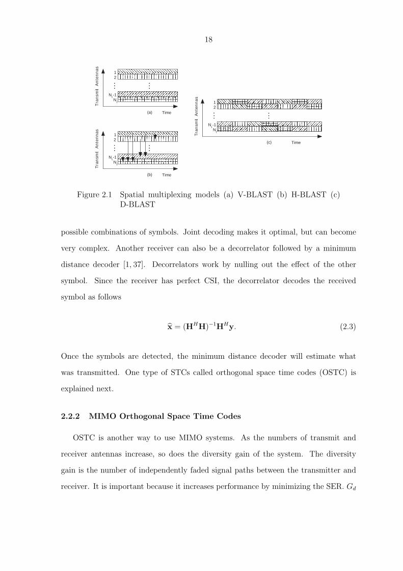
Figure 2.1 Spatial multiplexing models (a) V-BLAST (b) H-BLAST (c)

D-BLAST . . . . . . . . . . . . . . . . . . . . . . . . . . . . . 18

Figure 2.2 MISO system model . . . . . . . . . . . . . . . . . . . . . . . . 24

Figure 2.3 PSAM to estimate channel hnt [i], using F pilot symbols . . . . 26

Figure 2.4 The actual SER for different values of SNR using QPSK mod-

ulation with Nt = 3,N = 16, and BfTs = 0.05 . . . . . . . . . . 31

Figure 2.5 Analytical capacity curve vs. actual capacity curve with per-

fect CSI for N = 8, and BfTd = .2 . . . . . . . . . . . . . . . . 32

Figure 2.6 Capacity vs. delay Td for simulated perfect CSIR and ICE

curves, where N = 8, Nt = 3, and BfTs = .01 . . . . . . . . . . 35

Figure 3.1 OFDMA downlink using adaptive rate tracking with future

channel realizations, where N = 10, and β2 = .997 . . . . . . . 52

Figure 3.2 OFDMA downlink with adaptive rate tracking without future

channel realizations, where β1 = .997 . . . . . . . . . . . . . . 53

vi

Figure 3.3 Sum rate vs. PT for downlink OFDMA with rate tracking.

(dynamically adjusted w) N = 16, K = 4, and equal target

BERs (1e-3 for all users). User rate ratio follows [1 : 2 : 4 : 8].

L = 4 paths with a uniform power delay profile (PDP) . . . . 53

vii

ACKNOWLEDGEMENTS

I would like to express my thanks to those who helped me with my research and

the writing of this thesis. First and foremost, Dr. Yao Ma for his guidance, patience

and support throughout this entire project. Also, I would like to thank my committee

members for their efforts and contributions to this work: Dr. Zhengdao Wang and

Dr. Daji Qiao.

viii

ABSTRACT

Two promising candidates for beyond 3rd generation (B3G) and 4G communica-

tion standards are multiple input multiple output (MIMO) and orthogonal frequency

division multiple access (OFDMA) systems. OFDMA is a new technique that enables

multiple users to transmit parallel data streams, allowing a much higher data rate

than conventional systems, such as time division multiple access (TDMA) or code di-

vision multiple access (CDMA). Another research topic involving MIMO systems use

antenna arrays at both the transmitter and the receiver. By using multiple antennas,

the transmitter can adapt to the channel as it varies across time. This is accomplished

by using a codebook of beamforming vectors which are known to both the transmitter

and receiver. As the receiver acquires information about the channel, it calculates

which beamforming vector matches the channel the best. The receiver then sends

back the index of that vector to the transmitter. The symbol being transmitted is

multiplied by the beamforming vector and sent over the channel, this is known as

transmit beamforming (TB).

Transmit beamforming can not only increase performance in wireless MIMO sys-

tems, but also add increased performance when put in combination with other MIMO

systems like spatial multiplexing and space time codes. TB has advantages over other

MIMO schemes because by measuring the channel, one can use adaptive modulation

techniques to achieve a coding gain not obtainable without channel state informa-

tion (CSI). Past research assumed the feedback channel was error free and had no

delay. This isolated the effects of finite rate feedback. We assume there is delay in the

ix

feedback channel along with imperfect channel estimation (ICE) at the receiver. We

will show how detrimental these effects can be to TB’s performance and can not be

ignored.

OFDMA is a technique used to allow multiple users to communicate more reli-

ably. This is possible because OFDMA utilizes CSI which can increase capacity, and

decrease the total transmission power. With the amount of data being transmitted

over wireless channels today, the need for faster, more efficient transmission techniques

becomes essential. OFDMA uses adaptive modulation based on instantaneous chan-

nel conditions, to assign subcarriers to each user and allocate power to each carrier.

Past research has focused on many different methods for OFDMA, using sum rate

maximization techniques without fairness, or using short term fairness to improve the

Quality of Service (QoS) to each mobile station. This thesis will address important

issues that are missing, such as weighted SNR (w-SNR) based ranking with adap-

tive rate tracking to achieve long term rate proportional fairness (RPF) for downlink

OFDMA. Long term RPF is less strict and performs better than short term RPF which

is achieved through w-SNR ranking. The weight calculation can be implemented both

online or offline. If channel statistics are known offline, a fixed weight vector can be

calculated and used to allocate resources to each MS. When channel statistics are un-

known, adaptive rate tracking can be used to calculate the weight vector online. Then

resources are allocated based on each MS’s weight factor. This sum rate maximization

method with long term RPF and adaptive rate tracking has many advantages over

traditional schemes, including ease of implementation, allowing a higher data rate with

fairness, and allowing for distributed scheduling.

1

CHAPTER 1. Introduction

1.1 Background Information

Wireless Communication systems have been steadily evolving in order to improve

performance for users. Two promising candidates for beyond 3rd generation (B3G)

and 4G communication standards are multiple input multiple output (MIMO) and

orthogonal frequency division multiple access (OFDMA) systems. OFDMA is a new

technique that enables multiple users to transmit parallel data streams, allowing a

much higher data rate than conventional systems, such as time division multiple access

(TDMA) or code division multiple access (CDMA). This, in turn, could translate into

better cellular coverage and fewer dropped calls. Another research topic involving

MIMO systems use antenna arrays at both the transmitter and the receiver. Multiple

input refers to multiple antennas at the transmitter, and multiple output refers to

multiple antennas at the receiver. In addition, single input and single output refer

to a single antenna at the transmitter and receiver, respectively. By using multiple

antennas, the transmitter can adapt to the channel as it varies across time. This is

accomplished by using a codebook of beamforming vectors which are known to both

the transmitter and receiver. As the receiver acquires information about the channel, it

calculates which beamforming vector matches the channel the best. The receiver then

sends back the index of that vector to the transmitter. The symbol being transmitted

is multiplied by the beamforming vector and sent over the channel, this is known as

transmit beamforming (TB). The research in this thesis will investigate both OFDMA

2

and TB.

MIMO technology is essential in order to achieve high spectrum efficiency, enlarge

system coverage, and support high data rates [1]. With these multiple antenna sys-

tems, several different techniques can be implemented when transmitting data to the

receiver. The model for MIMO systems is shown in Figure 1.1. Along with MIMO,

some other multiple antenna systems are multiple input single output (MISO), or sin-

gle input multiple output (SIMO). One technique associated with MIMO systems is

spatial multiplexing (SM).

Spatial multiplexing (SM) uses a demultiplexer to divide the data into Nt differ-

ent streams, where Nt equals the number of transmit antennas. Each antenna then

transmits a different symbol. This technique uses the allowed spectrum much more

efficiently. STCs are less efficient because they only transmit one symbol per time

slot.

The STC technique involves three steps: encoding and transmission of data at the

transmitter, combining the data at the receiver, and the decision rule for detection.

Since the same signal is encoded differently, the receiver will get a redundant version

of it [1, 2]. The receiver can use this redundancy to correctly detect the transmitted

data; this is called receive diversity.

Receive diversity is very important because wireless channels suffer from a variety

of obstructions and refractions that cause scattering of the signals. The signals are

also distorted by noise from other signals being transmitted, and interference. If all

these distortions are severe enough, it is then impossible for the receiver to determine

the transmitted signal. This is why having multiple copies help in determining what

was transmitted [3]. Another way to transmit data is to use transmit beamforming.

3

1

2

N t

1

2

N r

.

.

.

.

.

.

h 1,1

h 1,2

h 2,2

h 2, Nr

h Nt , Nr

h 2,1

h Nt ,2

Figure 1.1 MIMO structure with Nt transmit antennas and Nr receive an-tennas

1.1.1 Transmit Beamforming

Transmit beamforming is very important to wireless communications because given

accurate channel conditions it can enhance performance of SM,STCs, or stand alone.

Refer to Table 1.1 for a list of abbreviations. TB uses information that the receiver

acquires about the channel conditions.

Table 1.1 List of abbreviationsMIMO Multiple Input Multiple OutputMISO Multiple Input Single OutputSIMO Single Input Multiple OutputTB Transmit BeamformingOFDMA Orthogonal Frequency Division Multiple AccessSTC Space Time CodesSM Spacial MultiplexingCSI Channel State InformationICE Imperfect Channel Estimation

The channel measurements can be obtained by sending out known pilot symbols

periodically from the transmitter to the receiver. The receiver can then use these

pilot symbols to estimate the channel at different time intervals. This is known as

pilot symbol-assisted modulation (PSAM), and is a good technique for rapidly fading

environments [4].

4

With TB for MISO systems, the different antenna elements at the transmitter

are designed to combine at the receiver adding a diversity gain of Nt over SISO sys-

tems. However, this gain requires that the transmitter have accurate knowledge of the

channel, because TB cannot be used to achieve capacity unless there is accurate CSI

available [5, 6].

Once the receiver knows the channel information, it can feedback this information

to the transmitter. The transmitter uses that information to best adapt to the channel.

In order to send all the information back, a large amount of bandwidth is necessary.

This is not very feasible in practical systems. The information needs to be compressed

due to the bandwidth constraint, and then sent back. This process is called finite rate

feedback. By increasing the number of feedback bits, it is possible to increase the

information supplied to the transmitter, which will lower the bit error rate (BER) of

the system. This works well with the first couple bits, but then the increase is minimal

with each subsequent bit [7]. Ideally, this feedback channel would be an error free,

no-delay channel, but that is not true in practice. Past research has only dealt with

this type of feedback channel, along with perfect CSI at the receiver.

Drawbacks to Transmit Beamforming

Each transmit antenna is associated with a single channel, or group of channels;

some channels are better than others. The receiver can acquire information about the

channel as it varies in time. There are two examples of this. One is when the receiver

knows the channel perfectly; this is referred to as the perfect channel state information

(CSI). Another example is when the receiver can only estimate the channel. This is

the most practical case, and is called imperfect channel estimation (ICE). Having ICE

at the receiver is more practical because having perfect CSI would either overload the

receiver, or the channel could fluctuate too rapidly to get an accurate estimate. There

are different types of ICE. One method is when the channel distribution is modeled

5

based on h ∼ N (µ, αI), where the mean µ is the estimate of the channel, and α is

the variance of the estimation error. A second approach is used when the channel

is varying too rapidly to obtain any instantaneous CSI, only channel statistics can

be obtained. Therefore, the channel is modeled based on h ∼ N (0,Σ). Here, since

the channel is changing too rapidly to acquire any accurate information, only the

covariance matrix Σ is used because its change is much slower [8, 9]. The benefit of

mean or covariance ICE is that capacity increases with more information about the

channel [10].

CSI is essential for TB because the transmitter requires accurate knowledge of the

channel. Some errors associated with TB include ICE, quantization errors, delays

during feedback, and errors caused by the feedback channel. Quantization errors are

incurred from using a finite number of bits to feed back the channel estimate to the

transmitter. Moreover, if the channel varies too rapidly, the channel will have changed,

and the feedback information becomes outdated by the time the transmitter is able

to use that information. Lastly, any errors induced by the feedback channel itself will

cause problems [9].

If the receiver does not know the actual channel realization, but only knows the

channel covariance matrix Σ, then it has no information about the attenuation of each

channel. It is only aware of directional information that can instead be used based

on the eigenvalues of Σ [11]. By using eigenvalue decomposition of Σ, the different

eigenvalues for each channel can be obtained. Beamforming along the largest of these

eigenvalues is optimal for increasing capacity. TB achieves capacity as the quality of

feedback improves in the mean feedback case, or the variation between eigenvalues of

the channel covariance matrix increases for covariance feedback [8]. In addition, by

increasing the number of antennas, TB schemes are better equipped to handle fading

channels [12–16].

6

Proposed method for Transmit Beamforming

The proposed method will take the delay into account, along with ICE at the

receiver. If there is no delay, the transmitter would have instantaneous knowledge of

the channel, and could adapt perfectly to it. However, with the delay and ICE, the

transmitter only knows past information about the channel estimates. It then has to

use that knowledge to adapt to the channel. This knowledge will cause some errors

because the channel changes with time. If the channel was not time varying, the

delay would not affect the performance. The outdated and imperfect CSI can be very

detrimental to the performance of the system, and needs to be taken into account.

When designing practical systems using TB, if the effects of delayed feedback and ICE

are neglected, the system could simply perform poorly, or in the worst case, completely

break down. Transmit beamforming has been proven to achieve optimal performance

in MISO systems based on signal to noise ratio (SNR) [17]. The second part of this

thesis discusses Orthogonal Frequency Division Multiple Access (OFDMA).

1.1.2 Orthogonal Frequency Division Multiple Access

There have been several different models implemented to allow for multiple access,

such as TDMA, frequency division multiple access (FDMA), and CDMA. TDMA

allocates different time slots to each user. FDMA works in a similar manner by

allocating a different frequency band to each user. CDMA assigns a different code to

each user. This allows multiple users access to the same frequency band and time slot

by encoding their transmissions. This works well because all other users look like noise

to everyone else. However, this type of flat fading environment cannot support high

data rates. These types of problems need to be addressed in 4G systems, in which

not only voice is being transmitted but also multimedia services such as MPEG video,

FTP, HTTP, and other data types as well [18,19].

Wideband CDMA (WCDMA) release 4 is intended to account for a wide range of

7

these services. The data rate associated with WCDMA is still too low. Therefore, an

upgrade to WCDMA called high speed downlink packet access (HSDPA) provides a

much higher data rate up to 14 Mbps, which makes it suitable for real time services [20–

22]. However, the Korean standard for wireless broadband internet (WiBro) utilizes

OFDMA and outperformed HSDPA by providing a higher data rate transmission in

multipath fading channels [22].

OFDMA is a technique used to allow multiple users to communicate more reliably.

This is possible because OFDMA utilizes CSI which can increase capacity, and decrease

the total transmission power. With the amount of data being transmitted over wireless

channels today, the need for faster, more efficient transmission techniques becomes

essential. OFDMA allows users to compete for resources to help eliminate resources

from being wasted. However, as the number of users in the system grows each year,

more people are battling to use the allocated bandwidth. That is why it is not only

important for future techniques to be efficient, but also fair. OFDMA could be unfair

to the users with weaker channels depending on how resources are allocated, which

is why rate proportional fairness (RPF) methods are being designed. Past research

involving short term RPF like in generalized processor sharing (GPS) assigns each user

a fixed weight. Then resources are allocated based on each user’s weight factor [23].

This method achieves short term fairness for each individual time slot, which is very

strict and unnecessary. The proposed method in this thesis achieves long term fairness

by assigning a weight vector to each user based on averaging their rate over multiple

time slots. Also, by utilizing adaptive rate tracking these weight factors for each user

can be updated online based on different quality of service requirements. Therefore,

research in finding the optimal solution to this fairness problem is essential and will

be discussed.

8

OFDMA System Model

OFDMA uses adaptive modulation based on instantaneous channel conditions, to

assign subcarriers to each user and allocate power to each carrier. Based on this, the

data rate is greatly improved over static resource allocation techniques. Different sub-

carriers experience different channel fades, which means they can transmit at different

data rates as well. However, the more fading the channel experiences, results in higher

gains being achieved.

In OFDMA, the allocated frequency band may be equally divided up into N dif-

ferent subcarriers. All users are possible candidates for resource allocation, and are

able to transmit using all time slots. The model for OFDMA is shown in Figure 1.2.

Extract Message for

User K

Sub carrier and

Power Allocation

Inverse Fourier Transform Modulator

( IFFT )

Frequency Selective Fading

Channel

Fourier Transform Demodulator

( FFT )

User 1 . . .

User K

User K

Add Cyclic Prefix for Guard Interval

Remove Cyclic Prefix

Extract Message for

User 1 User 1

.

.

.

Figure 1.2 Block diagram for OFDMA downlink system model

There can be any number of users in the system. Each user feeds their bit stream

into the subcarrier and power allocation block. The receiver knows the channel con-

ditions for each user, and can assign the carriers to maximize the total data rate of

the system. Once a set of subcarriers has been assigned to each user, then power

can be allocated to each carrier. The symbols are transformed into the time domain

using the inverse Fourier transform method (IFFT). Next, a cyclic extension is added

9

as a guard interval, which ensures orthogonality among the carriers. The signals are

then transmitted across the channel. At the kth user’s receiver, the guard interval is

removed to eliminate the intersymbol interference (ISI). This allows for higher data

rates because ISI distorts the signals making it very difficult for the receiver to de-

tect what was transmitted. The receiver then transforms the signals back into the

modulated symbols using the Fourier transform demodulator. Lastly, based on the

carrier set for the kth user, the message is pieced back together [24]. This scheme uses

dynamic allocation of resources and is optimal over static resource allocation.

Static resource allocation techniques result in poor performance because they do

not take CSI into account [25]. As a result, a large portion of carriers are wasted

because no other users can access them. Assigning a channel resources, whether it

be a time slot or frequency band to each user is not optimal. Using a dynamic

resource allocation approach like in OFDMA, causes less waste and achieves a higher

performance.

OFDMA Cellular Channel Model

The way mobile stations (MSs) communicate with the base station (BS) can be

seen in Figure 1.3. The uplink channel can be used to feedback channel conditions to

the BS. Since different users are located in different positions, their channel conditions

are independent of each other. Therefore, a scheduler can select which MSs are allo-

cated which resources to maximize the sum data rate, which is referred to as selective

multiuser diversity (SMuD). In almost all wireless applications, reliable data rates are

the most important factor in measuring the satisfaction of users [26]. There are many

advantages to OFDMA, such as high spectral efficiency, simple implementation by

FFT, low receiver complexity, and high data rate transmission over multipath fading

channels [1].

OFDMA is divided up into two steps. First, carriers are assigned to each user,

10

and second, power is allocated among the carriers. This provides the maximum total

data rate for the system. It was proven in [27] that exclusive carrier assignment

maximizes the data rate for downlink channel models over shared carrier allocation.

When multiple users share a specific carrier in shared carrier allocation, they end up

interfering with each other. As one user increases its transmit power, the interference

to other users is increased as well. The added interference makes this type of carrier

assignment suboptimal.

. . .

Downlink Channels

CSI Feedback

BS

MS 1

MS 2

MS n

Figure 1.3 OFDMA cellular channel model

The optimal method for OFDMA is to jointly allocate carriers and power. Joint

allocation methods are more complex for the uplink case than the downlink case

because of the different power constraints at the mobile stations. The method found

in [28] addresses this by calculating the data rate for each user and allocating resources

to the user with the largest data rate. This method may be optimal in sum rate, but

it is also unfair.

Proportional Fairness Techniques

In rate adaptive resource allocation, subcarriers and power are distributed in order

to achieve the maximum performance while maintaining proportional fairness among

11

users. There are two classes of optimization techniques which have been proposed in

OFDMA dynamic resource allocation literature. Margin adaptation (MA) achieves the

minimal overall transmit power given the constraints on the user’s data rates and error

rates. Rate adaptation (RA) maximizes the sum capacity with a total transmit power

constraint. In studying RA optimization techniques, several algorithms have been

proposed. Selective multiuser diversity with absolute SNR based ranking, referred to

as a-SNR SMuD OFDMA, is considered to be the conventional method that does not

take fairness into account. This can often provide an upper bound for proportional

fairness methods. Another method, called the Min-Max method, maximizes the worst

user’s capacity, but the overall capacity is sacrificed [29, 30]. There needs to be a

balance between achieving maximum sum capacity and fairness.

There are several different techniques to ensure proportional fairness. For example,

GPS scheduling can achieve a maximum sum rate while providing short term fairness.

In [23], GPS assigns each user a fixed weight instead of a fixed bandwidth, then

dynamically allocates carriers to each user according to their weight and traffic load.

Each user is guaranteed a minimum bandwidth proportional to its weight. If a user

does not use all of its guaranteed bandwidth, the unused portion is distributed to

other users in proportion to their weights. However, it is difficult to implement in

practice because of the following reasons. (1) Due to channel fading, the actual number

of subcarriers the system can support can be less than the theoretical number of

subcarriers because of poor channel gains. (2) If the number of backlogged sessions

becomes larger than the number of subcarriers, the system may not be able to allocate

the bandwidth to each user that GPS scheduling guarantees at each time slot.

Short term fairness ensures fairness for each individual time slot. Long term fair-

ness ensures a uniform average channel access probability (AAP), in which all users

have an equal number of assigned carriers over multiple time slots. Therefore, short

term fairness may be too strict and is unnecessary. Instead, long term fairness tech-

12

niques are adequate and perform better. In [31] and [32] a long term fairness approach

is taken called normalized SNR (n-SNR) SMuD. The normalized SNR equals the in-

stantaneous SNR divided by the average SNR. Unlike the a-SNR SMuD, which uses

the instantaneous SNR to assign carriers, the n-SNR scheme assigns carriers to the

users with the highest normalized SNR. Next, power can then be allocated to each

carrier.

The transmitter does not have infinite power for each channel, so there are a

couple of options to allocate power. One option is to simply divide the power equally

among each channel, whether the channel is reliable or not. This is called equal power

allocation (EPA), which is not optimal. By giving the poor channels the same amount

of power as the good channels, a large amount of power is being wasted. A better

approach is to give the better channels more power, and give the degraded channels

less power or no power at all. Using the Lagrangian method to solve the maximization

problem with respect to the power constraint, and solving the Karush-Kuhn-Tucker

(KKT) conditions, gives the optimal threshold. If a channel SNR does not reach this

threshold, then no power is allocated, and that channel is simply turned off. This

scheme is known as water filling (WF), because the better the channel, the more

power one can pour into it. WF is optimal for all SNR ranges [26, 28]. The proposed

method below takes a different approach to achieve long term fairness.

Proposed Method for OFDMA

The proposed method uses weighted SNR (w-SNR) based ranking with adaptive

rate tracking to achieve long term RPF for downlink OFDMA. There are several

different methods to obtain the optimal weight vector. (1) An offline algorithm is

provided to calculate the optimal weight factor when channel statistics are known.

(2) An online algorithm which utilizes adaptive rate tracking without future CSI to

find the optimal weight vector. (3) Adaptive rate tracking with future CSI is used

13

to obtain the optimal weight vector online as well. Next, depending on the different

users’ quality of service (QoS) requirements, a target RPF is obtained. The weight

factors for all users are then calculated based on this target RPF by any of the three

methods described above. Subcarriers and power are then allocated based on each

user’s weight factor. This sum rate maximization method with long term RPF and

adaptive rate tracking has many advantages over traditional schemes, including ease of

implementation, allowing a higher data rate with fairness, and allowing for distributed

scheduling.

Short term RPF schemes have a fixed weight factor where users are allocated

resources based on this weight factor alone. This happens regardless of their channel

conditions. A large amount of waste can occur because the channel cannot support

the data rate. The reverse is also true, a user could have a very good channel, but

is not allowed to utilize it because their weight factor is set to low. The proposed

adaptive rate tracking method takes temporal diversity into consideration allowing

more resources to be allocated beyond what is allowed by the user’s weight factor. This

is true if the user’s channel becomes better than their average value. The opposite

also holds, where if the user channel becomes poorer than their average value, less

resources are allocated. The following chapters are organized as follows.

1.2 Organization of Thesis

Chapter 2 focuses on transmit beamforming. It analyzes some MIMO techniques

and compares past TB research with the proposed method. Chapter 3 analyzes

OFDMA systems for the downlink case. It compares different approaches to OFDMA

and different resource allocation methods to the proposed method as well. Chapter 4

focuses on future work along with summarizing the results presented throughout this

work.

Notation: Bold upper and lower case letters denote matrices and column vectors,

14

respectively. | · | and ‖ · ‖ denote absolute value and a vector norm, respectively; (·)∗,(·)T , and (·)H denote the conjugate, transpose, and Hermitian transpose, respectively.

E{·} denotes expectation; IN denotes the identity matrix of size N; CN stands for

an N dimensional complex vector space; CN (µ,Σ) denotes the complex Gaussian

distribution with mean µ and covariance Σ.

15

CHAPTER 2. Transmit Beamforming

2.1 Introduction

Transmit beamforming can not only increase performance in wireless MIMO sys-

tems, but also add increased performance when put in combination with other MIMO

systems like SM and STC [33, 34]. TB has advantages over other MIMO schemes

because by measuring the channel, one can use adaptive modulation techniques to

achieve a coding gain not obtainable without CSI. It is difficult to use TB in a broad-

cast mode because TB is designed to transmit in a single direction like in point to

point links. Therefore, this chapter reviews SM,STCs, and past schemes involving

TB. Then we focus on the proposed method, TB with limited delayed feedback and

imperfect channel estimation. Past research assumed the feedback channel was error

free and had no delay. This isolated the effects of finite rate feedback. We assume

there is delay in the feedback channel along with ICE at the receiver. We will show

how detrimental these effects can be to TB’s performance and can not be ignored.

Both the transmitter and receiver have knowledge of the codebook that will be

used for TB. Once the receiver knows the channel, it will search through the codebook

to find the best beamforming vector and feedback the index of that vector to the

transmitter. The codebook is a matrix of size Nt × N , where Nt is the number of

transmit antennas and N is total number of beamforming vectors. If B is the number

of bits fed back, then N = 2B. Basically there are three different techniques that are

used with beamforming codebooks.

16

The first technique is called selection diversity transmission (SDT). This is where

the number of beamforming vectors equals the number of transmit antennas. The

codebook in this case is just the identity matrix INt . Here only the strongest channel

is chosen to transmit and all other antennas are turned off. The next technique is

called equal gain transmission (EGT). In this approach, the beamforming vectors are

divided up equally among them based on the number of transmit antennas, where

each beamforming vector w = 1√Nt

1Nt×1. The last approach is called maximum ratio

transmission (MRT). Here each beamforming vector can basically be any unit vector.

Transmitter complexity increases with these approaches with MRT being the most

complex, but system perfomance increases as well [35]. MRT is assumed throughout

this thesis when Nt is smaller than N . Besides TB, two additional schemes involving

MIMO systems are spatial multiplexing and space time codes, as discussed next.

2.2 Some Available MIMO Schemes

Spatial multiplexing and space time codes are two different ways to transmit data

over wireless channels. Spatial multiplexing utilizes all degrees of freedom (DoF) of

the channel, which uses the spectrum more efficiently. STCs transmit encoded data

over multiple antennas. This adds a diversity gain (Gd) to the system, and the receiver

has a better chance of properly decoding the message. Both schemes are important in

communications.

2.2.1 Spatial Multiplexing

Spatial multiplexing takes a stream of symbols and splits them up into smaller

independent streams. The number of streams depends on the number of transmit

antennas. Each antenna transmits a different stream. By increasing the numbers of

transmit antennas and receiver antennas in the system, there is an increase in DoF.

17

Degrees of freedom refer to the number of signals that can be reliably distinguished

at the receiver [36,37].

DoF = min(Nt, Nr) (2.1)

Spatial multiplexing starts off by sending a bit stream through an encoder and

converting them to a stream of complex symbols. Those symbols are then sent through

a demultiplexer. The demultiplexer divides the bit stream up into Nt independent

data streams, and sends them to each transmit antenna. Each independent data

stream is considered a layer [38]. There are three different ways to transmit using SM:

vertical Bell Labs layered space time (V-BLAST), horizontal BLAST (H-BLAST), and

diagonal BLAST (D-BLAST) (see Figure 2.1).

V-BLAST is a popular scheme because it is simple to implement. Each transmit

antenna sends an independent data stream or layer over the channel. H-BLAST can

be either coded or uncoded. If H-BLAST is uncoded it simply reduces to V-BLAST.

Coded H-BLAST is designed in such a way that each transmit antenna’s layer interferes

with the layers below it, and can not interfere with layers above it. D-BLAST works

differently because each of the layers are cycled periodically over each transmit antenna

during a specified time slot [39–41].

The model for spatial multiplexing V-BLAST is defined as

y = Hx + η, (2.2)

where y, H, x and η are the received signal, channel, data symbols, and additive

Gaussian noise matrices, respectfully. The received signal, data symbols, and noise

matrices are of size Nt× 1. There are several different techniques the receiver can use

to decode the data. Maximum likelihood (ML) uses joint decoding which compares all

18

. .

.

. .

.

1 2

N t -1 N

t

1 2

N t

(a)

(b)

. . .

1 2

N t

(c)

. . .

.

. .

. . .

N t -1

N t -1

Time

Time

Time

T r a

n s

m i t

A n

t e n

n a

s T

r a n

s m

i t A

n t e

n n

a s

T r a

n s

m i t

A n

t e n

n a

s Figure 2.1 Spatial multiplexing models (a) V-BLAST (b) H-BLAST (c)

D-BLAST

possible combinations of symbols. Joint decoding makes it optimal, but can become

very complex. Another receiver can also be a decorrelator followed by a minimum

distance decoder [1, 37]. Decorrelators work by nulling out the effect of the other

symbol. Since the receiver has perfect CSI, the decorrelator decodes the received

symbol as follows

x = (HHH)−1HHy. (2.3)

Once the symbols are detected, the minimum distance decoder will estimate what

was transmitted. One type of STCs called orthogonal space time codes (OSTC) is

explained next.

2.2.2 MIMO Orthogonal Space Time Codes

OSTC is another way to use MIMO systems. As the numbers of transmit and

receiver antennas increase, so does the diversity gain of the system. The diversity

gain is the number of independently faded signal paths between the transmitter and

receiver. It is important because it increases performance by minimizing the SER. Gd

19

is calculated by,

Gd = NtNr. (2.4)

This system starts off again by converting the bit stream into complex symbols.

The symbols are then encoded using an Alamuoti encoder [2, 37].

Table 2.1 Alamouti schemeTime slot 1 Time slot 2

x1 −x∗2x2 x∗1

The encoder transmits signals according to Table 2.1 when two transmit antennas

are used. The OSTC model is expressed as,

[y1 y2

]=

[h11 h12

]

x1 −x∗2

x2 x∗1

+

[n1 n2

]. (2.5)

Rearranging (2.5) will give

y1

y∗2

=

h11 h12

h∗12 −h∗11

x1

x2

+

n1

n∗2

, (2.6)

which is more intuitive when decoding the transmitted signals at the receiver. The

receiver can be a maximum likelihood decoder which takes the received symbols, and

using the channel information, decodes them to get the original symbols back. The

model for a maximum likelihood decoder is expressed as

x = arg min ‖ y −Hx ‖2. (2.7)

20

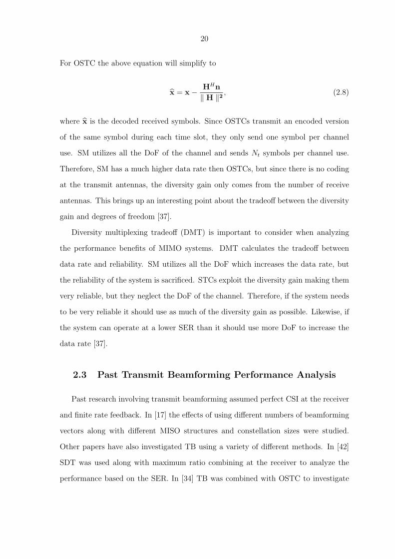
For OSTC the above equation will simplify to

x = x− HHn

‖ H ‖2 , (2.8)

where x is the decoded received symbols. Since OSTCs transmit an encoded version

of the same symbol during each time slot, they only send one symbol per channel

use. SM utilizes all the DoF of the channel and sends Nt symbols per channel use.

Therefore, SM has a much higher data rate then OSTCs, but since there is no coding

at the transmit antennas, the diversity gain only comes from the number of receive

antennas. This brings up an interesting point about the tradeoff between the diversity

gain and degrees of freedom [37].

Diversity multiplexing tradeoff (DMT) is important to consider when analyzing

the performance benefits of MIMO systems. DMT calculates the tradeoff between

data rate and reliability. SM utilizes all the DoF which increases the data rate, but

the reliability of the system is sacrificed. STCs exploit the diversity gain making them

very reliable, but they neglect the DoF of the channel. Therefore, if the system needs

to be very reliable it should use as much of the diversity gain as possible. Likewise, if

the system can operate at a lower SER than it should use more DoF to increase the

data rate [37].

2.3 Past Transmit Beamforming Performance Analysis

Past research involving transmit beamforming assumed perfect CSI at the receiver

and finite rate feedback. In [17] the effects of using different numbers of beamforming

vectors along with different MISO structures and constellation sizes were studied.

Other papers have also investigated TB using a variety of different methods. In [42]

SDT was used along with maximum ratio combining at the receiver to analyze the

performance based on the SER. In [34] TB was combined with OSTC to investigate

21

how performance can be improved over conventional OSTC for MIMO systems. In

[33] a different approach was used by combining TB with spatial multiplexing which

analyzed how using knowledge of the channel could improve performance. In [43]

the uplink cellular system is modeled with outdated CSI for the SIMO case. Also

in [44], an adaptive modulation scheme is used for MISO systems using channel mean

feedback with delay. In adaptive modulation schemes the transmitter not only adjusts

the BF vectors, but also the power allocation for each tranmit antenna and signal

constellation size to maintain a target SER. If the channel is in deep fade, then nothing

is transmitted. This type of scheme is less sensitive to channel imperfections than SISO

systems, but feedback delay significantly degraded the performance of the system.

In [17], an analytical lower bound was compared to the actual simulated curve.

This showed that the analytical lower bound was a tight approximation to the actual

SER curve for good beamformers across the entire SNR range. The channels were

assumed to be independent and identically distributed (i.i.d.), so the Grassmannian

line packing problem has been proven to provide the best beamformers in that case [45].

When designing good beamformers, maximizing the minimum chordal distance

between two beamforming vectors is the best option [17, 46]. The chordal distance is

defined as

d(wi,wj) = sin(θi,j) =√

1− |wHi wj|2, (2.9)

where θi,j denotes the angle between wi and wj. Good beamformers have been de-

signed in [47] for a number of different transmit antennas and codebook sizes. The

beamforming codebook, defined as

W = [w1 w2 ... wN ], (2.10)

consists of all the TB vectors. For example, the codebook for Nt = 2 and N = 4 is

22

W =

−.1612− j ∗ .7348 −.5135− j ∗ .4128

−.0787− j ∗ .3192 −.2506 + j ∗ .9106

−.2399 + j ∗ .5985 −.7641− j ∗ .0212

−.9541 .2996

T

. (2.11)

When the number of beamforming vectors is equal to the number of transmit

antennas, W simply reduces to the identity matrix of size Nt, INt , which is SDT. Once

these codebooks have been designed, the receiver having perfect CSI can compute

the optimal beamforming vector. Each beamforming vector is associated with an

index identifier, and the index of the optimal beamforming vector is fed back to the

transmitter. The transmitter then multiplies the TB vector w, with the symbol x to

be transmitted, and sends that over the channel. The MISO model is made up of Nt

transmit antennas and one receive antenna. The received symbol is defined as

y = wHhx + η, (2.12)

where η is complex Gaussian noise. The optimal TB vector is chosen based on the

instantaneous SNR for a Gaussian channel. The received instantaneous SNR is given

by

γ = |wHh|2 Es

N0

, (2.13)

where Es is the average symbol energy, and N0 is the variance of the noise. It can

be seen from (2.13) that in order to maximize the instantaneous SNR, one needs to

maximize |wHh|. Therefore, the optimal TB vector is defined as

wopt = arg max{wi}N

i=1

|wHh|2. (2.14)

23

The performance analysis for the SER with finite-rate feedback is reviewed next.

The first step is to identify the instantaneous SER based on a phase-shift keying (PSK)

constellation, which is defined as [48]

SER (γ) =1

π

∫ (M−1)πM

0

e−gPSKγ

sin2 θ dθ, (2.15)

where M is the constellation size and gPSK = sin2( πM

). To find the average SER, the

expectation of (2.15) with respect to the channel vector h needs to be taken. The

average SER is defined as SER = Eh{SER (γ)}. A good approximation for the

average SER lower bound is derived in [17],

SER LB =1

π

∫ (M−1)πM

θ=0

(1 +gPSKγ

sin2 θ)−1[1 + (1− (

1

N)

1Nt−1 )

gPSKγ

sin2 θ]1−Ntdθ. (2.16)

This equation has proven to be a very good lower bound for the average SER as

the graphs in [17] show for different Nt and N . As the number of vectors N increases,

the curve becomes closer to the case of perfect CSI at the transmitter (CSIT). Having

two bits provides adequate feedback for Nt = 2, therefore, adding an additional bit

does not yield a significant improvement in performance.

2.4 Transmit Beamforming with ICE, Delayed and Limited

Feedback

In this section, the SER will be analyzed based on delayed and limited feedback.

In [49] it is proven that as the delay increases, the SER increases as well, causing a

significant loss in performance. While these results have been studied in the literature,

they assumed perfect CSI at the receiver. While perfect CSI is often not possible in

practice due to channel fading and interference, the effects of ICE have not been

adequately studied and need to be considered [50]. We will show that ICE can cause a

24

loss in SNR at the receiver and cause the receiver to select a lower quality beamforming

vector.

2.4.1 System Model

The system model for TB with delay is shown in Figure 2.2, where x(t) is the in-

put data stream and the beamforming vectors associated with each transmit antenna

taking delayed feedback into account are w1(t|Td) to wNt(t|Td). The feedback delay

is Td > 0, and Td = nTs, where Ts is the symbol duration. The channels associated

with each transmit antenna are h1(t) to hNt(t). There are some assumptions regard-

ing the channel, h has i.i.d. entries, and follows the Rayleigh distribution, where

h ∼ CN (0, σ2hINt). Futhermore, the receiver does not have perfect knowledge of the

channel. Each data symbol x(t) is multiplied with the beamforming vector given as

X

X

X

X

w 1 (t|T

d )

w 2 (t|T

d )

w 3 (t|T

d )

w Nt

(t|T d )

x(t) Channel Estimator/ Detector

y(t)

Feedback Channel

h 1 (t)

h 2 (t)

h 3 (t)

h Nt

(t)

Delay T d

Figure 2.2 MISO system model

w(t|Td) = [w1(t|Td), ..., wNt(t|Td)]T , (2.17)

25

where w(t|Td) has unit norm ‖w(t|Td)‖ = 1. Each antenna transmits simultaneously,

and the received symbol is

y(t) = wH(t|Td)h(t)x(t) + η(t). (2.18)

The delayed instantaneous SNR is defined as

γ(t|Td) = |wH(t|Td)h(t)|2γs, (2.19)

where γs = Es

N0is the average symbol SNR defined in (2.13). Instead of using the

current channel to estimate the optimal beamforming vector, the outdated channel is

used.

wopt(t|Td) = arg max{wi}N

i=1

|wHi h(t− Td)|2 (2.20)

It can be seen from (2.20), that the BF vector that the transmitter uses is the

outdated vector. This will affect the instantaneous SNR and reduce performance.

Therefore, γ(t|Td) ≤ γ(t) for Td > 0. First, (2.19) can be decomposed into

γ(t|Td) = γh(t)(1− z)γs, (2.21)

where γh(t) = ||h(t)||2 and z is the square of the minimum distance between the

selected TB vector wopt(t|Td), and the normalized channel vector h(t) = h(t)||h(t)|| . z is

given by

z = mini

d2(wi(t|Td), h(t)) = d2(wopt(t|Td), h(t))

= 1− |wHopt(t|Td)h(t)|2. (2.22)

In order to analyze the effects ICE will have on the system, we will consider the PSAM

26

scheme.

2.4.2 Channel Estimation using PSAM

Pilot symbol assisted modulation transmits a number of pilot symbols every P

symbol durations. These pilot symbols are collected at the receiver and used to es-

timate the channel. We assume F pilot symbols are inserted to estimate h[i] =

[h1[i], ..., hNt [i]]T , where h[i] = h(iTs). Since the elements of h[i] are i.i.d., each chan-

nel is estimated separately for all Nt channels. Moreover, indices [i] and (t) denote

discrete time and continuous time indexes, respectively. In this scheme, hnt [i] is es-

timated separately for all 1 ≤ nt ≤ Nt. In order to estimate the channel coefficient

hnt [i], F pilot symbols are transmitted and can be expressed as an F × 1 vector

snt,PS = [s[i − (F − 1)P − int,off ], ..., s[i − int,off ]]T , where int,off = (1, ..., P − 1) is the

offset of the closest pilot symbol to the desired symbol being estimated (see Figure

2.3).

F pilot symbols

h nt [i]

i nt ,off P symbol duration

Figure 2.3 PSAM to estimate channel hnt [i], using F pilot symbols

The larger int,off is away from the desired symbol, the poorer the estimate will be.

For estimating h[i], it is assumed that the transmit antennas are only active one at a

time in the training mode to avoid interfering with each other. Therefore, int,off are

different for each antenna. The received signal at the pilot symbol positions are an

27

F × 1 vector ynt,PS , which is defined as

ynt,PS = (diag(snt,PS ))hnt,PS + ηnt,PS , (2.23)

where hnt,PS = [hnt [i − (F − 1)P − int,off ], . . . , hnt [i − int,off ]]T and ηnt,PS = [ηnt [i −(F −1)P − int,off ], . . . , ηnt [i− int,off ]]T are the complex channel gains and additive noise

at the pilot symbol positions, respectively. The pilot symbols are transmitted with

power PPS . Therefore, (2.23) reduces to ynt,PS =√

PPS hnt,PS + ηnt,PS . The channel

estimate for hnt [i] is expressed as

hnt [i] = gHnt,PS ynt,PS , (2.24)

where gnt,PS is a channel estimation filter. Using the estimated channel hnt [i] at time

t = iTs, the receiver calculates the optimal TB vector and feeds back that index to

the transmitter. The transmitter then uses that vector at time t = iTs + Td. Due to

the feedback delay. The optimal TB vector is calculated as follows,

wopt(t|Td) = arg max{wi}N

i=1

|wHi h(t− Td)|2. (2.25)

Based on this PSAM model, we consider the minimum mean squared error chan-

nel estimator (MMSE-CE), because it can best minimize the estimation MSE. The

MMSE-CE filter is expressed as

gnt,mmse = R−1yPS rh,yPS , (2.26)

where rh,yPS = E[h∗ntynt,PS ] =

√PPS [Rh[(F−1)P+int,off ], . . . , Rh[int,off ]]T , and Rh[m] =

E[hnt [i]h∗nt

[i −m]] is defined as the channel temporal correlation coefficient. It is as-

sumed that the channel conditions are slowly time varying, according to Clark’s fad-

28

ing spectrum, therefore, Rh[m] = σ2hJ0(2πBfTsm). J0(x) is the zeroth-order Bessel

function, and Bf is the Doppler fading bandwidth [37]. Also, from (2.26) RyPS =

E[ynt,PS yHnt,PS ] is a Toeplitz matrix defined as the auto correlation matrix of ynt,PS .

The first row of RyPS is given by [PPS Rh[0] + N0, PPS R∗h[P ], . . . .PPS R∗

h[P (F − 1)]].

With the effects of ICE, and limited and delayed feedback to the system, quality will

be severely degraded. To demonstrate this effect, the channel model with limited and

delayed feedback errors will be analyzed next, followed by considering the effects of

ICE at the receiver.

2.4.3 SER Lower Bound for Limited and Delayed Feedback

We propose to model the channel with delay alone as

h(t) = ρdh(t− Td) + ed(t), (2.27)

where ρd = E[hl(t)h∗l (t − Td)] is the correlation coefficient between the true channel

and the outdated channel for {l = 1, ..., Nt}. In addition, ed(t) is the error vector with

distribution ed(t) ∼ CN (0, σ2h(1− |ρd|2)INt). Substituting (2.27) into (2.19), the new

instantaneous SNR with delay and limited feedback can be written as

γ(t|Td, z) = |wHopt(t|Td)[ρdh(t− Td) + ed(t)]|2γs

= |ρdwHopt(t|Td)h(t− Td) + wH

opt(t|Td)ed(t))|2γs. (2.28)

Taking into account that |wHopt(t|Td)h(t−Td)|2 = (1−z)γh(t−Td), where γh(t−Td) =

‖h(t−Td)‖2. Also, γh(t−Td) is a chi-square variable with 2Nt degrees of freedom [37].

Therefore, the moment generating function (MGF) of φγh(t−Td)(s) is 1(1−sσ2

h)Nt. It can

29

be seen from [51] that the MGF of (2.28) is

Φγ(t|Td,z)(s) =(1− ρ2

d(1− z)[s−1γ−1s,h − (1− |ρd|2)]−1)−Nt

1− sγs,h(1− |ρd|2)

=[1− sγs,h(1− |ρd|2)]Nt−1

[1− sγs,h(1− |ρd|2z)]Nt=

(1− ss1

)Nt−1

(1− ss2

)Nt, (2.29)

where s1 = 1γs,h(1−|ρd|2)

, s2 = 1γs,h(1−|ρd|2z)

, and γs,h = γsσ2h adds in the effect of channel

gain. By taking the expectation of (2.15) with respect to γh and z, where γ = γh(1−z)γs, the average SER of M-PSK modulation is given by

SER =

∫ ∞

γh=0

∫ z0

z=0

∫ (M−1)πM

0

1

πe−gPSKγh(1−z)γs

sin2 θ fγh(γh)fz(z)dθdγhdz, (2.30)

where fγh(γh) and fz(z) are the probability density functions (PDFs) of γh and z,

respectively. The cumulative distribution function (CDF) of z, which is defined as

Fz(z), needs to be found. This has proven to be a very difficult task, but a tight upper

bound on the CDF of z has been derived in [17] for good TB codebooks. In [17] the

tight upper bound of Fz(z) was found to be

Fz(z) = NzNt−1, z ≤ z0, (2.31)

where z0 = ( 1N

)1

Nt−1 . This upper bound holds for 0 ≤ z ≤ z0, and ∼ represents the

upper bound approximation. Next, by differentiating (2.31) an approximate PDF of

z is given by fz(z) = N(Nt − 1)zNt−2, for z ≤ z0. The MGF of γh is defined as

E[e−sγh ] =

∫ ∞

γh=0

fγh(γh)e

−sγhdγh. (2.32)

Therefore, substituting (2.29), where s = −gPSK

sin2 θand fz(z) into (2.30), then inte-

30

grating over z will give the SER lower bound as

SERLB =1

π

∫ (M−1)πM

θ=0

[1 +gPSKγs,h

sin2 θ(1− |ρd|2)]Nt−1

1 +gPSKγs,h

sin2 θ

×[1 + (1− |ρd|2( 1

N)

1Nt−1 )

gPSKγs,h

sin2 θ]1−Ntdθ, (2.33)

Furthermore, we assume the channel conditions are varying according to Clarke’s

fading spectrum, ρd = J0(2πBfTd), and |ρd| does not decrease to zero but fluctuates

around zero as Td → ∞. This can be seen in the numerical results with perfect CSI

at the receiver (CSIR).

The numerical results in Figure 2.4 show the loss in performance for different SNR

values, where Nt = 3, BfTs = 0.05, and N = 16 are assumed. It is shown that as

Td increases, the SER increases as well and then fluctuates around a constant value

as Td →∞. Figure 2.5 shows how delayed feedback can significantly reduce capacity

over all SNR ranges. This simulation compares the analytical curve to the actual

simulated curve when there are N = 8 TB vectors, and BfTd = 0.2 for the delay.

Next, the results for ICE at the receiver will be investigated.

2.4.4 Capacity of Proposed TB Method with ICE, Limited and Delayed

Feedback

By factoring ICE into the channel model without delay, the model becomes

h(t) = ρe(σh

σh

)h(t) + eh(t), (2.34)

where ρe =E[hl(t)h

∗l (t)]

σhσh

is the correlation coefficient between elements of h(t) and h(t).

Also, eh(t) is the error vector with distribution eh(t) ∼ CN (0, σ2h(1 − |ρe|2)INt). By

adding a delay to equation (2.34), and combining it with (2.27), the new channel

31

0 5 10 15 2010

−3

10−2

10−1

100

Td (T

d = nT

s)

SE

R

BfT

s=0.05

N=16

SNR =0 with csiSNR =5 with csiSNR =10 with csi

Figure 2.4 The actual SER for different values of SNR using QPSK modu-lation with Nt = 3,N = 16, and BfTs = 0.05

model with ICE, limited and delayed feedback can be expressed as

h(t) = ρdρe(σh

σh

)h(t− Td) + e(t), (2.35)

where e(t) = ρdeh(t − Td) + ed(t). The effects of ICE will not only hurt the quality

of feedback information, but will also cause a loss in SNR. This loss factor is derived

as [52,53]

β =|ρhw |2

(1− |ρhw |2)Ntγ + 1, (2.36)

where ρhw is the normalized channel coefficient between the actual channel hw =

wopt(t|Td)h(t) and the estimated channel hw = wopt(t|Td)h(t). Also, ρhw depends on

the PSAM scheme chosen along with system parameters. Combining equations (2.35)

and (2.36), then substituting them into (2.19) will provide the received SNR including

32

0 2 4 6 8 10 12 141

1.5

2

2.5

3

3.5

4

4.5

5

5.5

6

Average Symbol SNR (dB)

Cap

acity

(bi

ts/s

/Hz)

N =8 BfT

d = 0 Analytical

N =8 BfT

d = 0 Simulated

N =8 BfT

d = .2 Analytical

N =8 BfT

d = .2 Simulated

Figure 2.5 Analytical capacity curve vs. actual capacity curve with perfectCSI for N = 8, and BfTd = .2

ICE.

γ(t|Td) = |wHopt(t|Td)[ρdρe(

σh

σh

)h(t− Td) + e(t)]|2βγs (2.37)

Also, (2.37) can be simplified to

γ(t|Td) = |ρtotwHopt(t|Td)h(t− Td) + etot(t)|2βγs, (2.38)

where ρtot = ρdρe(σh

σh), and etot(t) = wH

opt(t|Td)e(t). In order to derive the MGF of

γ(t|Td), which is defined as φγ(t|Td,z)(s) = E[esγ(t|Td,z)], it needs to be expressed in a

non-central Gaussian quadratic form conditioned on h(t− Td) [54]. This will give the

conditional MGF φγ(t|Td,z)(s|h). Therefore, the complex Gaussian quadratic form of

γ(t|Td) conditioned on h(t − Td) equals v∗βγsv, where v = ρtotwHopt(t|Td)h(t − Td) +

etot(t) ∼ CN (ρtotwHopt(t|Td)h(t−Td), σ

2h(1−|ρtot|2)). Following the results for Gaussian

33

quadratic forms in [54], the conditional MGF of γ(t|Td) is obtained as

φγ(t|Td,z)(s|h) =exp{|ρtot|2|wH

opt(t|Td)h(t− Td)|2[(βγs)−1s−1 − σ2

h(1− |ρtot|2)]−1}1− sβγsσ

2h(1− |ρtot|2) (2.39)

Finally, φγ(t|Td,z)(s|h) will need to be averaged over h(t−Td) to obtain the average

MGF φγ(t|Td,z)(s).

φγ(t|Td,z)(s) =[1− sβγs,h(1− |ρtot|2)]Nt−1

[1− sβγs,h(1− |ρtot|2z)]Nt

=[1− s

s1]Nt−1

[1− ss2

]Nt, (2.40)

where s1 = 1βγs,h(1−|ρtot|2)

and s2 = 1βγs,h(1−|ρtot|2z)

. See appendix for the complete proof.

It can be seen from (2.40), that with no delay, and perfect CSIR, ρtot = 1 so ρhw = 1,

then β = 1, therefore, the MGF reduces to

φγ(t|Td=0,z)(s) =1

[1− sγs,h(1− z)]Nt. (2.41)

Next, with full rate feedback, imperfect receiver CSI, and the delay, the MGF

becomes

φγ(t|Td,z=0)(s) =[1− sβγs,h(1− |ρtot|2)]Nt−1

[1− sβγs,h]Nt

. (2.42)

Based on (2.40)-(2.42), one observes that the effects of delayed feedback and ICE at

the receiver can significantly reduce the systems performance. Finally, by averaging

out the quantization error, the MGF of γ(t|Td) can be obtained. In order to average

out the effects of z, the approximate PDF of z needs to be used, then the average

34

approximate MGF of γ(t|Td) can be found as

φγ(t|Td)(s) =

∫ z0

0

φγ(t|Td,z)(s)fz(z)dz

=

∫ z0

0

N(Nt − 1)zNt−2[1− sβγs,h(1− |ρtot|2)]Nt−1

[1− sβγs,h(1− |ρtot|2z)]Ntdz

= N(Nt − 1)[1− sβγs,h(1− |ρtot|2)]Nt−1

∫ z0

0

zNt−2

[1− sβγs,h(1− |ρtot|2z)]Ntdz

= N(Nt − 1)[1− sβγs,h(1− |ρtot|2)]Nt−1

∫ z0

0

zNt−2

[a + bz)]Ntdz, (2.43)

where a = 1− sβγs,h and b = sβγs,h|ρtot|2. With the integral written in this manner,

it can be solved by using the closed form expression

∫zNt−2

(a + bz)Ntdz =

zNt−1(a + bz)1−Nt

a(Nt − 1). (2.44)

Based on this equality, the average MGF of γ(t|Td) becomes

φγ(t|Td)(s) =[1− sβγs,h(1− |ρtot|2)]Nt−1

(1− sβγs,h)[1− sβγs,h(1− |ρtot|2z0)]Nt−1. (2.45)

By using (2.45) the capacity of the system with limited and delayed feedback, along

with ICE at the receiver, can now be analyzed. A good approximation is calculated

by

C ≈∫ ∞

0

∫ z0

0

log(1 + x)fγ(t|Td)(x)fz(z)dzdx

=

∫ ∞

0

log(1 + x)fγ(t|Td)(x)dx, (2.46)

where fγ(t|Td)(x) is the approximate PDF of γ(t|Td) by taking the inverse Laplace

transform of (2.45). Based on these calculations it can be seen in Figure 2.6 how

detrimental limited, delayed feedback, and ICE at the receiver can be to the system.

This demonstrates the importance of takeing these factors into account when designing

35

a TB system to be used in practice.

0 5 10 15 20 25 30 35 400

1

2

3

4

5

6

7

8

Td (T

d = nT

s)

Cap

acity

(bi

ts/s

/Hz)

BfT

s=0.01

N=8

SNR =5 with CSIRSNR =10 with CSIRSNR =15 with CSIRSNR =5 with ICESNR =10 with ICESNR =15 with ICE

Figure 2.6 Capacity vs. delay Td for simulated perfect CSIR and ICEcurves, where N = 8, Nt = 3, and BfTs = .01

36

CHAPTER 3. Orthogonal Frequency Division Multiple

Access

3.1 Introduction

In this chapter, the OFDMA cellular structure along with various multicarrier

allocation strategies will be studied. Past research has focused on many different

methods for OFDMA, using sum rate maximization techniques without fairness, or

using short term fairness to improve the Quality of Service (QoS) to each mobile

station. This was achieved by using rate adaptive techniques to maximize the overall

data rate, while maintaining short term fairness by adding an extra constraint where

each MS’s rate Rk follows a predetermined rate ratio R1 : · · · : Rk = α1 : · · · : αk.

This thesis will address important issues that are missing, such as w-SNR ranking

SMuD with long term RPF and adaptive rate tracking (ART). Long term RPF is less

strict and performs better than short term RPF which is achieved through w-SNR

ranking. The weight calculation can be implemented both online or offline. If channel

statistics are known offline, a fixed weight vector can be calculated and used to allocate

resources to each MS. When channel statistics are unknown, adaptive rate tracking

can be used to calculate the weight vector online. Then resources are allocated based

on each MS’s weight factor.

The OFDMA cellular channel model is comprised of a BS, MSs, uplink channels,

and downlink channels. These channels are used as a way for MSs and BSs to com-

municate with each other. For example, when assigning resources, the BS sends out

37

pilot symbols to the MSs on the downlink channels. The MSs then feed back their CSI

to the BS on the uplink channels. Finally the BS communicates with the MSs on the

downlink channels again with the assigned resources. For the uplink case, the power

constraint for each MS needs to be considered when allocating resources. This is due

to the various requirements for each MS. However, for the downlink channels there is

only one power constraint. Therefore, in assigning resources the optimal method of

joint power and subcarrier assignment is more complex for the uplink case.

3.2 Past Research Involving Multicarrier Based Resource

Allocation Startegies

Multicarrier based resource allocation falls under two catagories: static and dy-

namic assignment. Static assignment refers to fixed allocation strategies, where each

user is assigned a certain subset of carriers pertaining to a fixed time slot or frequency

band. With regards to dynamic assignment, any user can be assigned any subcarrier

pertaining to any time slot or frequency band depending on their channel strength.

Different systems use different allocation techniques depending on what the system

is trying to accomplish. Static resource allocation provides the least complicated re-

ceiver designs because no feedback CSI is needed. However, this causes an abundance

of waste when channel conditions become poor. Dynamic assignment on the other

hand causes less waste, but could possibly increase complexity at the receiver side

and for the scheduler. There are a couple of different strategies for static channel

assignment.

3.2.1 Static Resource Assignment

There are many different kinds of static methods to assign carriers. These methods

range from the simplest round robin (RR) technique, to the more involved methods

38

such as, allocating a specific frequency band or time slot to a specific user [24,55]. For

OFDMA, RR allocates each time slot, one at a time, to each MS. RR does not take

any type of CSI into account. It evenly divides up the carriers, but does not come

close to being optimal [55].

An alternate static assignment method would be to allow each user to transmit

during a specific time slot that is unique to each MS. This provides each MS an equal

share of time to transmit data, but does not take into account any CSI. The MSs are

allowed to use any carriers during their allocated time slot.

Another approach designates each MS carriers for a particular bandwidth. There-

fore, the MSs can transmit during all time slots. However, due to the fading charac-

teristics of the channel, the capacity over the short term for static allocation methods

would vary widely as a result of a user’s channel being in a deep fade.

Since the users are dispersed throughout the cell, each MS’s channel is different

and independent, resulting in different fading and path loss effects. Path loss can be

expressed as a ratio between transmitted and received power [56]. The smaller the

path loss, the better. There are many factors contributing to path loss, these include

both BS and MS antenna heights, each MS’s distance from the BS, the subcarrier’s

frequency, and the terrain surrounding each MS. Therefore, multicarrier resource al-

location will be significantly affected by all of these factors.

When allocating resources both sum rate maximization and fairness among users

need to be considered. Static resource allocation techniques perform poorly in these

areas because they do not take CSI into account. The resources are allocated equally,

but due to the effects of fading channels and path loss the data rate suffers greatly.

Dynamic resource allocation deems the more interesting case.

39

3.2.2 Dynamic Carrier, Power and Rate Assignment

Dynamic resource assignment takes CSI into account in order to optimally allo-

cate resources to each user with minimal waste. Resources can be allocated a few

different ways. Carriers can be assigned using exclusive carrier assignment (ECA)

or shared carrier assignment (SCA). Resources can also be allocated based on each

MS’s SNR alone or rate maximization techniques. Finally, fairness metrics can also

be implemented to ensure each MS gets an equal share of the resources.

ECA only allows one MS to utilize a given carrier at any one time. This ensures

there is no interference between MSs since all carriers are orthogonal with each other.

In order to maximize the data rate, it was proven in [27] that ECA is optimal for

centralized schemes described in this thesis.

SCA allows more than one MS to be assigned a given carrier. This causes prob-

lems since interference becomes an issue. As one MS increases transmit power, the

signal-to-interference-plus-noise ratio (SINR) of the other MSs goes down. This added

interference also decreases the overall data rate when compared to ECA. SCA is more

suitable for ad hoc networks where interference between MSs could be significantly

less [57]. The basic scheme allocating resources using ECA is described next.

Allocating carriers based on each MS’s SNR, is referred to as absolute SNR (a-

SNR) ranking based SMuD scheme [31]. This method maximizes capacity without

being fair to each MS. When allocating resources dynamically, it is essential to know

each MS’s CSI. Utilizing this information, the base station computes each MS’s SNR,

and assigns the carrier to the MS with the highest SNR value. Once all carriers have

been assigned, power can be allocated using either EPA or WF.

For EPA, the transmit power is divided equally among each carrier. Since the

channels are assumed to be Rayleigh fading they will experience different channel

gains. Therefore, this is not optimal since assigning the weaker channels the same

amount of power as the stronger channels will result in a lot of power being wasted.

40

Instead, using the WF method to allocate power is a better approach.

WF utilizes the Lagrangian function to maximize the sum rate under the total

power constraint. Since the sum rate is a concave function, taking the derivative of

the Lagrangian function with respect to power, and setting the result to zero gives

a series of equations called KKT conditions. Solving these equations with regards

to the maximum power constraint yields an optimal SNR threshold, termed as the

waterfilling level. Based on this threshold, power can than be allocated to each carrier.

This method has proven to be optimal when allocating power [28].

Channel dependant scheduling techniques use CSI to calculate each MS’s data rate

and then allocate resources depending on which MS has the largest rate. This tech-

nique is shown in [29], where power and carriers are allocated jointly. Since the data

rate is dependant on the product of channel SNR and transmit power. These con-

straints need to be taken into account together which greatly increases the complexity

of the system. Dynamic allocation techniques also need to be fair.

Fairness metrics ensure each MS gets an equal share of the resources allocated.

This can be accomplished in the short term, or long term. Short term fairness ensures

fairness among MSs for each individual time slot. Long term fairness allows each MS

access to an equal number of carriers over a period of time [58]. There are different

ways of implementing short term or long term fairness.

Proportional fair scheduling (PFS) transmits to the user with the largest normal-

ized data rate or received SNR [32]. In [58] PFS is implemented for both short and

long term fairness cases. It was proven that long term fairness outperformed the more

strict short term fairness based on n-SNR ranking. PFS schemes are able to ensure

fairness, but they are not able to adjust for different quality of service requirements.

Since a lot of different multimedia services are being transmitted over wireless

channels, some MSs require higher data rates then others. RPF allocates resources to

ensure each MS’s data rate follows a predetermined rate ratio vector [30]. Therefore,

41

resources are allocated based on each MS’s weight factor, where more resources are

allocated to higher weights.

3.2.3 Past Research Involving Rate Proportional Fairness Techniques

RPF techniques are needed to ensure fairness among MSs. In [29] and [30] sum

rate maximization techniques were used along with RPF to ensure short term fairness.

The algorithm in [29] is much like the a-SNR ranking case, except a constraint is added

where each MS’s rate Rk follows a predetermined rate ratio R1 : · · · : RK = α1 : · · · :αK . In the first step, each MS’s power and carriers are set to zero, where N is the

total number of carriers, and K is the total number of MSs. Next, each MS finds a

carrier that maximizes their SNR, where γk = maxn γk,n. Each user is then assigned

that specific carrier, and power is allocated to that user. Power is divided up using

EPA, and based on these initial values, each MS’s rate is calculated by

Rk =B

Nlog(1 + Pkγk), (3.1)

where B is the total bandwidth. After each user is assigned one carrier, the rest of

the carriers will be assigned using the RPF technique [29]. Out of the rates calculated

in (3.1), the ith MS with the smallest ratio is selected to be assigned the next carrier.

Ri

αi

≤ Rk

αk

(3.2)

From the remaining N −K carriers, the carrier n that maximizes that MS’s SNR

γi,n is assigned to MS i. Their power is then increased by Pi = Pi + Pt

N, and the sum

rate for MS i is calculated. However, before the sum rate can be calculated, power

has to be allocated to each carrier using the WF technique.

The algorithm for WF uses the Lagrangian function to maximize the sum rate

subject to (s.t.) the total power constraint. The optimization model for downlink rate

42

maximization is defined as

max{Pn}

∑nεSi

log(1 + Pn(t)γi,n(t)), s.t.∑nεSi

Pn(t) ≤ Pi, (3.3)

where γi,n(t) is the channel SNR of the selected user at carrier n, and Si is a set of all

carriers assigned to the ith mobile station. The Lagrangian function is then used to

maximize (3.3), which is expressed as

L(λ(t), {Pn(t)}) =∑nεSi

log(1 + Pn(t)γi,n(t))− λ(t)

(∑nεSi

Pn(t)− Pi

), (3.4)

where λ(t) is the Lagrangian multiplier. The index t will be dropped for simplicity, for

example Pn(t) = Pn, unless otherwise stated. By taking the derivative of (3.4) with

respect to (w.r.t.) {Pn}, and setting the resulting equations equal to zero, we get the

maximum value for Pn because the capacity is a concave function.

dLdPn

=γi,n

1 + Pnγi,n

− λ = 0 (3.5)

Rearranging (3.5), and solving for Pn gives

P ∗n =

(1

λ− 1

γi,n

)+

s.t.∑nεSi

P ∗n ≤ Pi, (3.6)

where (x)+ is the maximum value between 0 and x. Solving (3.6) for λ gives the

solution for optimal SNR threshold level giving by

λ =Neff

Pi +∑

nεSi

1γi,n

, (3.7)

where, Neff ≤ N . The power for MS i is then allocated by using (3.6). The sum rate

43

is calculated by

Ri =∑nεSi

B

Nlog(1 + P ∗

nγi,n). (3.8)

The process then starts over and compares each MS’s rate ratio using equation

(3.2) to assign the next carrier. This type of joint subcarrier and power allocation

technique is a suboptimal approach to maximizing the sum rate, while achieving short

term fairness. Other research has been done to maximize the sum rate while achieving

long term fairness. In [59], they use the normalized SNR (n-SNR) ranking to help

improve performance for the TDMA model, while [31] and [58] used n-SNR ranking

for the OFDMA model. It was shown in [31], that the n-SNR ranking scheme with long

term fairness outperformed the more strict short term fairness scheme. Normalized

SNR ranking achieves long term fairness by averaging each MS’s SNR over multiple

time slots. By finding the average SNR γk,n, for each MS k = 1, . . . , K, and each

carrier n = 1, . . . , N , each MS’s SNR can be normalized, γk,n =γk,n

γk,n. Based on this

normalized SNR, the MS k∗ with the highest n-SNR value is selected for each carrier.

γk∗,n = maxn{γ1,n, . . . , γK,n} (3.9)

Once each carrier has been assigned to each user, the power is then allocated by

either EPA or WF. If EPA is used, then the sum rate becomes

R =N∑

n=1

B

Nlog(1 + γk∗,n

Pt

N), (3.10)

where γk∗,n is the instantaneous SNR of user k∗ at carrier n. If the WF method is

used to allocate power, then each carrier will be allocated a certain amount of power

P ∗n based on KKT conditions for WF. When each carrier is allocated power, the sum

44

rate will be

R =N∑

n=1

B

Nlog(1 + γk∗,nP ∗

n). (3.11)

This method ensures a long term fairness by normalizing each MS’s SNR before

allocating carriers. That way the effects caused by noise and path loss can be canceled

out, and MS’s with weaker channels will get the same amount of resources allocated

to them as the MS’s with stronger channels. However, there is no way of tracking the

different QoS requirements for different traffic types such as MPEG video or HTTP.

Instead, we propose to use a weighted SNR (w-SNR) ranking SMuD method with long

term RPF and adaptive rate tracking to account for this.

3.3 Long Term RPF with w-SNR Ranking and Adaptive

Rate Tracking

In the proposed method, each MS can be assigned a different weight factor to

fit for the different traffic types and QoS requirements. Depending on what those

requirements are, MS’s with a larger weight will be allocated more resources then

MS’s with a smaller weight. By using long term fairness, each MS is guaranteed a

fair share of the available resources. In addition, by using adaptive rate tracking,

when a MS’s channel becomes better than average more resources can be allocated to

that user by updating their weight factor online, or vice versa. This type of adaptive

rate tracking can significantly increase the sum rate for the system. There are three

methods that can be implemented to find the optimal weight vector (wopt). The first

method calculates the SNR weight vector for all MS’s offline when channel statistics

are known. The second method uses adaptive rate tracking without future CSI online

to calculate each MS’s data rate, and then dynamically adjusts each MS’s weight

factor until wopt is found. Lastly, the third method uses adaptive rate tracking with

45

future CSI online to calculate wopt. Finally, when wopt is obtained by any of the three

methods, the scheduler allocates resources online according to each MS’s weight to

maintain the target RPF. The system model for the OFDMA downlink case will be

explained next.

3.3.1 System Model

Assume the downlink OFDMA has K MSs and N total available carriers. Note, all

variables defined here are independent of any variables defined earlier in the transmit

beamforming section. Also, the time index t will be dropped for simplicity. The

channels are independent between MS’s, and follow a Rayleigh distribution. The

instantaneous SNR of user k, at subcarrier n, is defined as

γhk,n =

|hk,n|2Nk,n

, (3.12)

where hk,n is the complex channel gain, and Nk,n is the band-limited noise power. The

BS has a maximum power expressed as Pt, which is divided among all the N carriers.

Therefore, Pn is the power allocated to the nth carrier, and

N∑n=1

Pn ≤ Pt (3.13)

is the total power constraint. Due to WF some carriers may be wasted. Also, Sk is

the set of carriers allocated to user k, subject to

K⋃

k=1

Sk ⊂ {1, . . . , N}.

Based on these variables, the sum rate for the system is expressed as

K∑

k=1

N∑n=1

ak,nRk,n, (3.14)

46

where ak,n = {0, 1} denotes if user k is assigned carrier n, and∑K

k=1 ak,n ≤ 1 is based

on the fact that each carrier n can be assigned to at most one user. Moreover, Rk,n is

the kth MS’s data rate at carrier n, defined as

Rk,n =B

Nlog(1 + Pk,nξkγ

hk,n), (3.15)

where ξk is the SNR gap function, which equals one for ergodic capacity, and ξk =

−1.5log(5Pe,k)

for the continuous rate QAM constellation [60]. Pe,k is defined as the target

bit error rate (BER) for user k. In addition,∑K

k=1

∑Nn=1 ak,nPk,n = Pt is the total

power constraint based on ECA. Using the SNR channel assignment method, it can

be seen from (3.15), that in order to maximize the sum rate, each MS’s SNR should be

maximized at each carrier. Therefore, by combining the SNR gap function with each

MS’s instantaneous SNR, the new SNR is defined as γk,n = ξkγhk,n. The BS calculates

this quantity based on the CSI from each user. By adding in RPF and using ECA, the

sum rate maximization technique subject to power and long term fairness constraints

is

max{ak,n}{Pk,n}

∑Kk=1

∑Nn=1 ak,nRk,n

s.t.∑K

k=1

∑Nn=1 ak,nPk,n ≤ Pt

{R1 : · · · : RK} = {α1 : · · · : αK}.

ECA means∑K

k=1 ak,n ≤ 1, and the average rate of the kth MS is Rk = Et[Rk], where

Et[·] means taking the expectation with respect to t. The sum rate for MS k is given

by

Rk =∑nεSk

Rk,n. (3.16)

Once all the carriers have been assigned, power can be allocated by either EPA, or

47

WF methods.

3.3.2 Resource Allocation and Different Methods Involving Optimal Weight

Vector Calculation

The proposed method is divided up into three parts. The first part finds the

optimal weight vector offline using known channel statistics. The second part utilizes

ART without future CSI to calculate the optimal weight vector online. The Third

method uses ART with future CSI to calculate the optimal weight vector online as

well. Once wopt has been obtained by any of the three methods, resources can be

allocated accordingly.

Online Allocation of Resources Using w-SNR Ranking Method

For weighted SNR ranking, the weight factor wk is multiplied by the normalized

instantaneous SNR. Each MS’s weight factor is calculated based on the target RPF

{R1 : · · · : RK} = {α1 : · · · : αK}. Therefore, the adjusted normalized SNR is defined

as

zk,n =wkγk,n

γk

, (3.17)

where the average channel gain γk = E[γk,n], and the weight factor is subject to∑K

k=1 wk = K. Allocation of resources depends on the normalized adjusted SNR

value found in (3.17). Since zk,n =wkγk,n

γk, then γk,n =

zk,nγk

wk. The w-SNR ranking

selection at carrier n is defined as

k∗ = arg maxk{z1,n, . . . , zK,n}. (3.18)

When all carriers have been assigned. Power is allocated by either EPA or WF.

Once all resources have been allocated to each MS, the average weighted rate vector

48

R(w) can be obtained. The average rate for MS k∗ at carrier n can be calculated

based on EPA as follows,

Rk∗,n(w) = E

[B

Nlog

(1 + γk∗,n

Pt

N

)]. (3.19)

The average sum rate for MS k is simply Rk(w) =∑

nεSkRk∗,n(w). For the WF

method, λ can be obtained from (3.6). Therefore, the average rate based on WF is

expressed as

Rk∗,n(w) = E

[B

Nlog (1 + γk∗,nP ∗

n)

], (3.20)

and the average sum rate is calculated the same as the EPA case. Once the average

individual rate is obtained, the optimal weight vector can be calculated.

Offline Weight Vector Calculation

The weight vector is needed to allocate resources to each MS. The steps taken

to find the optimal weight vector follow an iterative method based on each MS’s

average rate. The weight vector and average weighted rate vector are defined as

w = [w1, . . . , wK ]T and R(w) = [R1(w), . . . , RK(w)]T , respectively. Also, the average

sum rate is

Rtot(w) =K∑

k=1

Rk(w). (3.21)

To achieve a target RPF, the prespecified rate ratio vector α = [α1, . . . , αK ]T is

set where

K∑

k=1

αk = 1. (3.22)

49

Therefore, the target RPF is RRPF(w) = Rtot(w)α. Based on these values for each

MS, the iterative approach defines a rate ratio vector as

r = [r1, . . . , rK ]T =

[R1

α1

, . . . ,RK

αK

]T

. (3.23)

This vector is then normalized by r = Kr∑Kk=1 rk

, where∑K

k=1 rk = K. The target RPF is

attained when r = 1K×1. In order to accomplish this, the optimal weight vector wopt

needs to be found using the following steps, where {s = 1, 2, . . .} is the index for each

step. Therefore, from r(s) = [r1(s), . . . , rK(s)]T , both the maximum and minimum

normalized rate ratio need to be obtained.

Furthermore, the error in the normalized rate ratio vector is defined as e(s) =

rmax(s)− rmin(s). When the magnitude of error |e(s)| is smaller then some arbitrarily

small value (εe > 0), then the target RPF is achieved. For the first step, s = 1,

set w(1) = 1K×1, then find the average weighted rate vector R(w). From that we

calculate the normalized rate ratio vector r(1), and find the error e(1).

e(1) = rmax(1)− rmin(1) (3.24)

Compare the magnitude of the error to the threshold as follows,

|e(s)| < εe. (3.25)

If (3.25) is true then stop and wopt is found, otherwise find the MS whose current RPF

is the smallest and largest out of all the MS’s.

kmin = arg mink

rk

kmax = arg maxk

rk (3.26)

50

Next, these weight vectors can be updated by

wk(s + 1) = wk(s)− β(s)e(s),

where β(s) is a scalar value that decreases as s increases. The remaining elements of

w(s+1) are the same as w(s), where∑K

k=1 wk(s) = K for all s. Based on the updated

weight vector w(s + 1), recalculate R(w) and r(s + 1), increase s by one and find the

error again. If (3.25) holds true, then the optimal weight vector has been obtained,

otherwise go back to (3.26) and increase s by one. The optimal weight vector is then

used in the proposed method for w-SNR ranking, which achieves the desired long term

RPF. The algorithm for finding wopt is provided next.

1. Set s = 1 and w = 1K×1.

2. Calculate R(w) and then the rate ratio vector, r =[

R1

α1, . . . , RK

αK

]T

.

3. Normalize the rate ratio vector r = Kr∑Kk=1 rk

.

4. For r(s) = [r1(s), . . . , rK(s)]T , find rmin(s) and rmax(s).

5. Calculate error factor e(s), where e(s) = rmax(s)− rmin(s).

6. Compare the error factor with threshold εe, where |e(s)| < εe. If inequality holds

true then stop and output wopt, otherwise continue on to step 7.

7. Find kmin = arg mink rk, and kmax = arg maxk rk.

8. Update these weight vectors where wk(s + 1) = wk(s)− β(s)e(s), while leaving

the remaining elements of w(s) alone, as long as∑K

k=1 wk(s) = K for all s.

9. Based on w(s + 1) calculate R(w) and r(s + 1).

10. Increment s by one, and go back to step 4.

51

Adaptive Rate Tracking w-SNR Method with and without Future CSI

ART involves either using future channel realizations, or not using future CSI

to make sure each MS’s rate is following the optimal rate ratio for each user. This

assumption allows the effects of ART to be analyzed along with the benefits of future

CSI. Each MS’s rate can be tracked without future CSI as follows,

Rk(t) = βkRk(t− Ts) + (1− βk)Rk(t). (3.27)

If future CSI is taken into account then each MS’s rate is tracked by

Rk(t) = βkRk(t− Ts) +(1− βk)

N[Rk(t), . . . , Rk(t + (N − 1)Ts)], (3.28)

where βk is called the forgetting factor, and N is the number of future channel real-

izations. These forgetting factors can be adjusted to how much future estimates effect

the average rate for MS k. The larger the forgetting factor means the larger the sliding

window size becomes, where βk = 1 − 1Tc

and Tc is the window size. Once Rk(t) is

known for each MS, a MMSE approach is used to calculate the error given by

ek(t) =Rk(t)−Rk,tar (t)

Rk,tar (t)=

Rk(t)

Rk,tar (t)− 1, (3.29)

where Rk,tar (t) = Rtot(t)αk. Next, the weight factor can be updated using

wk(t + Ts) = wk(t)− βek(t), (3.30)

where β is a scaler value.

This online approach is very beneficial when channel statistics cannot be obtained

offline. ART can be shown in Figures 3.1 and 3.2. In Figure 3.1 each MS’s rate is

tracked and compared to a statistical optimal rate with future CSI included, where

52

the number of channel realizations N = 10 and βk = .997. Figure 3.1 can also be

compared to Figure 3.2, where ART does not use future CSI and βk = .997. It can

be seen that by utilizing future CSI, the time needed to converge to the optimal rate

is dramatically reduced. Figure 3.3 shows different w-SNR schemes with and without

ART, where N = 16, K = 4, α = [1 : 2 : 4 : 8], and L = 4 paths with a uniform power

delay profile (PDP).

0 500 1000 1500 2000 25000

0.5

1

1.5

2

2.5

3

3.5

4

Time Slot Index

Indi

vidu

al R

ate

Solid lines: Stat. optimal

Dashed lines: Adap. Rate tracking

User 1User 2User 3User 4

Figure 3.1 OFDMA downlink using adaptive rate tracking with futurechannel realizations, where N = 10, and β2 = .997

53

0 500 1000 1500 2000 25000

0.5

1

1.5

2

2.5

3

3.5

4

4.5

Time Slot Index

Indi

vidu

al R

ate

Solid lines: Stat. optimalDashed lines: Adap. Rate tracking

User 1User 2User 3User 4

Figure 3.2 OFDMA downlink with adaptive rate tracking without futurechannel realizations, where β1 = .997

0 5 10 15 20 25 300

10

20

30

40

50

60

70

80

PT (dB)

Sum

Rat

e

N=16, K=4

Uniform PDP

w−SNR, stat. opt., simu

w−SNR, stat. opt., Ana.

w−SNR, RT, simu

short−term fairness, simu

Figure 3.3 Sum rate vs. PT for downlink OFDMA with rate tracking. (dy-namically adjusted w) N = 16, K = 4, and equal target BERs(1e-3 for all users). User rate ratio follows [1 : 2 : 4 : 8]. L = 4paths with a uniform power delay profile (PDP)

54

CHAPTER 4. Conclusion

4.1 Summary

This thesis showed what the effects of limited delayed feedback, along with ICE at

the receiver, has on transmit beamforming. This model demonstrated that both finite

rate and delayed feedback, can significantly reduce performance as the delay increases.

This was shown for both SER and capacity curves. With just a moderate delay, the

SER increased substantially for medium to high SNR ranges, where capacity decreased

over all SNR ranges. Capacity is very sensitive to the effects of ICE at the receiver.

If the delay in feedback increases, with ICE at the receiver, capacity can be reduced

to practically zero. Therefore, these effects can not be ignored for future systems.

OFDMA systems do have issues that need to be addressed as well. OFDMA

has proven to be a very good candidate for 4G systems, but it can also be unfair

to potential users. Therefore, the conventional method a-SNR SMuD proved to be

an upper capacity bound for systems trying to improve fairness. Short term rate

proportional fairness was too strict, and a more long term RPF method was found

to be adequate. Based on these facts, w-SNR ranking with SMuD and long term

RPF proved that it could maximize performance and provide long term RPF for

every user. Furthermore, by adding in adaptive rate tracking, each MS’s rate can be

tracked and compared against their optimal rate to ensure the system is operating

within the required range. It was shown that by taking future CSI into account, the

convergence time to the optimal rate was greatly reduced when compared to adaptive

55

rate tracking without utilizing future CSI. Therefore, the proposed method has proven

to outperform other methods for maximizing capacity and achieving long term fairness

for each MS.

4.2 Future Work

The proposed methods in this thesis for transmit beamforming and OFDMA can

be expanded for future work in a couple of different ways. TB assumed each channel

was independent and followed a Rayleigh distribution. This assumption needs to be

expanded to the point where the channels are correlated with each other. Furthermore,

future work is being done to improve the pilot symbol assisted modulation method.

Rather than having only pilot symbols for past channel realizations, to estimate the

current channel at time t, the pilot symbols can be divided into two groups. Half

of the pilot symbols can be inserted for past estimates of the current channel, along

with the other half of the pilot symbols inserted with predicted future estimates of

the current channel. This will in turn, give a much better estimate, improving the

effects that ICE has on the system. Moreover, with these predicted future values of the

channel, a more suitable TB vector can be selected to overcome the effects feedback

delay produces. Also, precoding can be implemented to further increase gains, and

also reduce the receiver complexity. Lastly, this thesis only considered MISO systems,

TB with finite rate, delayed feedback, and ICE at the receiver, should be analyzed

in regards to MIMO systems as well, to observe what occurs when the number of

antennas are increased at the receiver.

Likewise, there is a great deal of future work needing to be accomplished for

OFDMA. The proposed method for OFDMA assumed perfect channel knowledge of

future channel realizations, when adaptive rate tracking is performed. For practical

systems, these future channel realizations need to be predicted as stated in the TB

case. With these predicted estimates, adaptive rate tracking will converge to the

56

optimal rate much faster.

Also, A MISO system was considered in the downlink case because of practical

reasons. Most cellular phones have only one antenna, future phones will be equipped

with multiple antennas. Therefore, the MIMO case should be considered as well.

Furthurmore, this thesis considered only a centralized scenario, where MSs communi-

cate with the BS alone, and vice verse. Instead, a multihop network, where MSs can

relay messages from other MSs to the BS should also be considered.

In addition, combining OFDMA with TB would make for an interesting research

problem. This could further improve performance in terms of coding and multiplex-

ing gains. However, these topics are beyond the scope of this thesis, but should be

addressed in future research.

57

APPENDIX

Moment Generating Function of Received SNR Including

ICE

The complex Gaussian quadratic form of γ(t|Td) conditioned on h(t − Td) equals

v∗βγsv, where v = ρtotwHopt(t|Td)h(t−Td)+etot(t) ∼ CN (ρtotw

Hopt(t|Td)h(t−Td), σ

2h(1−

|ρtot|2)). Following the results for Gaussian quadratic forms in [54], the conditional

MGF of γ(t|Td) is obtained.

φγ(t|Td,z)(s|h) =exp{|ρtot|2|wH

opt(t|Td)h(t− Td)|2[(βγs)−1s−1 − σ2

h(1− |ρtot|2)]−1}1− sβγsσ

2h(1− |ρtot|2) (A.1)

Based on the quantization error z, it was shown earlier that |wHopt(t|Td)h(t − Td)|2 =

(1− z)||h(t− Td)||2, where γh(t− Td) = ||h(t− Td)||2. Therefore, with this change of

variables, the new equation with quantization error becomes

|wHopt(t|Td)h(t− Td)|2 = (1− z)γh(t− Td). (A.2)

Since γh(t− Td) is a scaled chi-square variable with 2Nt degrees of freedom, the MGF

becomes φγh(t−Td)(s) = E[esγh(t−Td)] = 1(1−sσ2

h)Nt. Substituting (A.2) into (A.1) the

conditional MGF becomes

φγ(t|Td,z)(s|h) =exp{|ρtot|2(1− z)γh(t− Td)[(βγs)

−1s−1 − σ2h(1− |ρtot|2)]−1}

1− sβγsσ2h(1− |ρtot|2) , (A.3)

where s = |ρtot|2(1− z)((βγs)−1s−1 − σ2

h(1− |ρtot|2))−1. Substituting s into (A.3) and

58

taking the expectation with respect to the channel h, the average MGF is defined as

φγ(t|Td,z)(s) = E[esγh(t−Td)

1− sβγsσ2h(1− |ρtot|2) ]

=(1− sσ2

h)−Nt

1− sβγsσ2h(1− |ρtot|2) . (A.4)

By replacing s with its actual value and simplifying (A.4), the average MGF becomes

φγ(t|Td,z)(s) =[1− sβγs,h(1− |ρtot|2)]Nt−1

[1− sβγs,h(1− |ρtot|2z)]Nt

=[1− s

s1]Nt−1

[1− ss2

]Nt, (A.5)

where s1 = 1βγs,h(1−|ρtot|2)

and s2 = 1βγs,h(1−|ρtot|2z)

.

59

BIBLIOGRAPHY

[1] T. B. M. Gadze, D. Nogulic, “Smart antenna systems for broadband technolo-gies,” 48th International Symposium, pp. 171–174, 7-9 June 2006.

[2] S. Alamouti, “A simple transmit diversity technique for wireless communica-tions,” IEEE J. Sel. Areas Commun., vol. 16, pp. 1451–1458, Oct. 1998.

[3] N. S. V. Tarokh and A. R. Calderbank, “Space-time codes for high data ratewireless communication: Performance criterion and code construction,” IEEETransactions on Information Theory, vol. 44, pp. 744–765, Mar. 1998.

[4] S. Zhou and G. B. Giannakis, “Optimal transmitter eigen-beamforming andspace-time block coding based on channel correlations,” IEEE Transactions onInformation Theory, vol. 49, pp. 1673–1690, Jul. 2003.

[5] M. D. T. A. Narula, M. J. Lopez and G. W. Wornell, “Efficient use of sideinformation in multiple-antenna data transmission over fading channels,” IEEEJ. Sel. Areas Communications, vol. 16, pp. 1423–1436, Oct. 1998.

[6] J. H. Winters, “The diversity gain of transmit diversity in wireless systems withrayleigh fading,” IEEE Transactions on Veh. Technol., vol. 47, pp. 119–123, Feb.1998.

[7] S. Z. P. Xia and G. B. Giannakis, “Multi-antenna adaptive modulation withbeamforming based on bandwidth-constrained feedback,” IEEE Transactions onCommunications, vol. 53, pp. 526–536, Mar. 2005.

[8] E. Visotsky and U. Madhow, “Space-time transmit precoding with imperfectfeedback,” IEEE Transactions on Information Theory, vol. 47, pp. 2632–2639,Sep. 2001.

[9] S. Zhou and G. B. Giannakis, “Optimal transmitter eigen-beamforming andspace-time block coding based on channel mean feedback,” IEEE Transactionson Signal Process., vol. 50, pp. 2599–2613, Oct. 2002.

[10] N. J. A. Goldsmith, S. A. Jafar and S. Vishwanath, “Capacity limits of MIMOchannels,” IEEE J. Sel. Areas Commun., vol. 21, pp. 684–702, Jun. 2003.

[11] H. Boche and E. A. Jorswieck, “Optimal power allocation for MISO systems andcomplete characterization of the impact of correlation o the capacity,” Proc. Int.Conf. Acoust., Speech, and Signal Process., pp. 373–376, Apr. 2003.

60

[12] S. Simon and A. Moustakas, “Optimizing MIMO antenna systems with channelcovariance feedback,” IEEE J. Sel. Areas Commun., vol. 21, pp. 406–417, Apr.2003.

[13] S. A. Jafar and A. Goldsmith, “On optimality of beamforming for multiple an-tenna systems with imperfect feedback,” Proc. IEEE int. Symp. Information The-ory, p. 321, June 2001.

[14] A. Moustakas and S. Simon, “Optimizing multiple-input single-output MISOcommunications systems with general Gaussian channels: Non-trivial covarianceand nonzero mean,” IEEE Transactions on Information Theory, vol. 49, pp. 2770–2780, Oct. 2003.

[15] H. Sampath and A. Paulraj, “Linear precoding for space-time coded systems withknown fading correlations,” IEEE Commun. Lett., vol. 6, pp. 239–241, Jun. 2002.

[16] R. Blum, “MIMO with limited feedback of channel state information,” Proc. ofIEEE int. Comf. Acoutst., Speech, and Signal Process., vol. 4, pp. 89–92, Apr.2003.

[17] G. B. G. S. Zhou, Z. Wang, “Quantifying the power loss when transmit beam-forming relies on finite rate feedback,” IEEE Transactions on Wireless Commun.,vol. 4, pp. 1948–1957, Jul. 2005.

[18] R. B. Theodore S. Rappaport, A. Annamalai and W. H. Tranter, “Wirelesscommunications: past events and a future perspective,” IEEE Commun. Mag.,vol. 40, pp. 148–161, May 2002.

[19] V. Singh and V. Sharma, “Efficient and fair scheduling of uplink and downlink inIEEE 802.16 OFDMA networks,” IEEE Wireless Communications and Network-ing Conference, vol. 2, pp. 984–990, Apr. 2006.

[20] W. X. Robert Love, Amitava Ghosh and R. Ratasuk, “Performance of 3GPP highspeed downlink packet access HSDPA,” IEEE Vehicular Technology Conference,vol. 5, pp. 3359–3363, 26-29 Sept. 2004.

[21] P. Li and W. Wu, “The comparison of performances when WCDMA and HS-DPA coexist in two different environments,” International Conference on Wire-less Communications Networking and Mobile Computing, vol. 2, pp. 824–828,23-26 Sept. 2005.

[22] J.-C. K. Simon Shin, Chan-koo Kang and S.-H. Oh, “The performance comparisonbetween WiBro and HSDPA,” International Symposium on Wireless Communi-cation Systems, pp. 346–350, 5-7 Sept. 2005.

[23] X. S. Jun Cai and J. W. Mark, “Downlink resource management for packet trans-mission in OFDM wireless communication systems,” IEEE Trans. on WirelessCommunications, vol. 4, pp. 1688–1703, July 2005.

61

[24] C. Y. Wong and R. S. Cheng, “Multiuser OFDM with adaptive subcarrier,bit, and power allocation,” IEEE Journal on Selected Area in Communications,vol. 17, pp. 1747–1758, Oct. 1999.

[25] W. Yu and J. M. Cioffi, “FDMA capacity of gaussian multiple-access channelswith ISI,” IEEE on Transactions Communications, vol. 50, pp. 102–111, Jan.2002.

[26] G. Song and Y. G. Li, “Adaptive subcarrier and power allocation in OFDMbased on maximizing utility,” IEEE Vehicular Technology Conf., pp. 905–909,Apr. 2003.

[27] J. Jang and K. B. Lee, “Transmit power adaptation for multiuser OFDM sys-tems,” IEEE Journal on Selected Areas in Communications, vol. 21, pp. 171–178,Feb. 2003.

[28] Y. H. Keunyoung Kim and S.-L. Kim, “Joint subcarrier and power allocation inuplink OFDMA systems,” IEEE Communications Letters, vol. 9, pp. 526–528,June 2005.

[29] C. Mohanram and S. Bhashyam, “A sub-optimal joint subcarrier and power al-location algorithm for multiuser OFDM,” IEEE Communications Letters, vol. 9,pp. 685–687, Aug. 2005.

[30] J. G. A. Zukang Shen and B. L. Evans, “Adaptive resource allocation in multiuserOFDM systems with proportional rate constraints,” IEEE Trans. on WirelessComm., vol. 4, pp. 2726–2737, Nov. 2005.

[31] Y. Ma, “Proportional fair scheduling for downlink OFDMA,” Proc. IEEE ICC’07,pp. 4843–4848, June 2007.

[32] L. Yang and M.-S. Alouini, “Performance analysis of multiuser selection diver-sity,” IEEE Trans. on Vehicular Technology, vol. 55, pp. 1848–1861, Nov. 2006.

[33] D. Love and J. R. W. Heath, “Limited feedback precoding for spatial multiplexingsystems,” Proc. Global Telecommunications Conf., vol. 4, pp. 1857–1861, Dec.2003.

[34] F. Jongren and M. Skoglund, “Utilizing quantized feedback information in orthog-onal space-time block coding,” Proc. Global Telecommunications Conf., vol. 2,pp. 995–999, Nov. 27-Dec. 1 2000.

[35] D. J. Love and R. W. Heath, “Equal gain transmission in multiple-input multiple-output wireless systems,” IEEE Transactions on Communications, vol. 51,pp. 1102–1110, Jul. 2003.

[36] J. Robert W. Heath and A. J. Paulraj, “Switching between diversity and mul-tiplexing in MIMO systems,” IEEE Trans. on Commun., vol. 53, pp. 962–968,June 2005.

62

[37] D. Tse and P. Viswanath, Fundamentals of Wireless Communication. CambridgeUniversity Press, 2005.

[38] R. N. Rui Zhang, Ying-Chang Liang and J. M. Cioffi, “Approaching MIMO-OFDM capacity with per-antenna power and rate feedback,” IEEE Journal onSelected Areas in Communications, vol. 25, pp. 1284–1297, Sept. 2007.

[39] G. D. G. P. W. Wolniansky, G. J. Foschini and R. A. Valenzuela, “V-blast: Anarchitecture for realizing very high data rate over the rich scattering wirelesschannel,” URSI International Symposium on Signals, Systems, and Electronics,pp. 295–300, 29 Sept.-2 Oct. 1998.

[40] J. Choi, “Capacity/throughput optimization for H-BLAST with SC receiver overMIMO channels,” IEEE Transactions on Wireless Channels, vol. 7, pp. 1016–1024, March 2008.

[41] M. J. G. C. P. Gerald J. Foschini, Dmitry Chizhik and R. A. Valenzuela, “Anal-ysis and performance on some basic space-time architectures,” IEEE Journal onSelected Areas in Communications, vol. 21, pp. 303–320, Apr. 2003.

[42] B. G. S. Thoen, L. Van der Perre and M. Engels, “Performance analysis ofcombined transmit-SC/receive-MRC,” IEEE Transactions on Communications,vol. 49, pp. 5–8, Jan. 2001.

[43] M. J. V. K. N. Lau and Y. Liu, “Cross layer design of uplink multi-antennawireless systems with outdated csi,” IEEE Transactions on Wireless Commun.,vol. 5, pp. 1250–1253, Jun. 2006.

[44] S. Zhou and G. B. Giannakis, “Adaptive modulation for multiantenna transmis-sions with channel mean feedback,” IEEE Transactions on Wireless Commun,vol. 3, pp. 1626–1636, Sep. 2004.

[45] R. H. H. J. H. Conway and N. J. A. Sloane, “Packing lines, planes, etc,: Packingsin grassmannian space,” Exp. Math, vol. 5, no. 2, pp. 139–159, 1996.

[46] J. D. J. Love, R. W. Heath and T. Strohmer, “Grassmannian beamforming formultiple-input multiple-output wireless systems,” IEEE Transactions on Infor-mation Theory, vol. 49, pp. 2735–2747, Oct. 2003.

[47] D. Love, http://dynamo.ecn.purdue.edu/ djlove/grass.html. Jun. 2005.

[48] M. K. Simon and M. S. Alouini, Digital communications over generalized fadingchannels: A unified approach to the performance analysis. New York: Wiley,2000.

[49] Y. Ma and D. Zhang, “Error rate of transmit beamforming with delayed andlimited feedback,” IEEE Global Telecommunications Conference, pp. 4071–4075,26-30 Nov. 2007.

63

[50] A. L. Yao Ma and R. Schober, “Predictive feedback for transmit beamformingwith delayed feedback and channel estimation errors,” 2008. submitted for pub-lication.

[51] A. L. Yao Ma, Dongbo Zhang and Z. Wang, “Error rate of transmit beamformingwith delayed and limited feedback,” IEEE Trans. on Wireless Communications,2008. submitted for publication.

[52] R. S. Yao Ma and S. Pasupathy, “Performance of M-PSK with GSC and EGCwith Gaussian weighted errors,” IEEE Transactions on Vehicular Technology,vol. 54, pp. 149–162, Jan. 2005.

[53] Y. Ma and J. Jin, “Effect of channel estimation errors on M-QAM with MRC andEGC in nakagami fading channels,” IEEE Transactions on Vehicular Technology,vol. 56, pp. 1239–1250, May 2007.

[54] A. Mathai and S. Provost, Quadratic forms in random variables: Theory andapplications. New York 10016: Marcel Dekker, 1992.

[55] F. K. L. M. C. Oghenekome Oteri, Nicolae Chiurtu and A. Paulraj, “Studies indownlink spectral efficiency of OFDMA networks with MIMO and opportunisticscheduling,” IEEE Global Telecommunications Conf., pp. 1–6, Nov. 2006.

[56] D. C. M. S. V.S. Abhayawardhana, I.J. Wassell and M. Brown, “Comparison ofempirical propagation path loss models for fixed wireless access systems,” IEEEVehicular Technology Conference, vol. 1, pp. 73–77, 30 May-1 June 2005.

[57] A. L. Yao Ma and D.-I. Kim, “Sum rate optimization of multi-cell cognitiveradio networks with spectral mask constraint,” Proc. IEEE Global Comm, 2008.accepted for publication.

[58] Y. Ma, “Rate-maximization for downlink OFDMA with proportional fairness,”IEEE Trans. Veh. Technol., 2007.

[59] M.-S. A. Lin Yang and D. Gesbert, “Further results on selective multiuser diver-sity,” Proc. MSWiM’04, pp. 25–30, Oct. 25-30 2004.

[60] A. Goldsmith, Wireless Communications. Cambridge University Press, 2005.