Analysis of Trace Finite Element Methods for

Surface Partial Differential Equations

Arnold Reusken∗

Bericht Nr. 387 Marz 2014

Key words: trace finite elements, error analysis, elliptic surface equation

AMS Subject Classifications: 58J32, 65N15, 65N30

Institut fur Geometrie und Praktische Mathematik

RWTH Aachen

Templergraben 55, D–52056 Aachen (Germany)

∗Institut fur Geometrie und Praktische Mathematik, RWTH-Aachen University, D-52056 Aachen,Germany; e-mail: reusken@igpm.rwth-aachen.de

ANALYSIS OF TRACE FINITE ELEMENT METHODS FORSURFACE PARTIAL DIFFERENTIAL EQUATIONS

ARNOLD REUSKEN∗

Abstract. In this paper we consider two variants of a trace finite element method for solvingelliptic partial differential equations on a stationary smooth manifold Γ. A discretization erroranalysis for both methods in one general framework is presented. Higher order finite elements aretreated and rather general numerical approximations Γh of the manifold Γ are allowed. Optimalorder discretization error bounds are derived. Furthermore, the conditioning of the stiffness matricesis studied. It is proved that for one of these two variants the corresponding scaled stiffness matrixhas a condition number ∼ h−2, independent of how Γh intersects the outer triangulation.

Key words. trace finite elements, error analysis, elliptic surface equation

AMS subject classifications. 58J32, 65N15, 65N30

1. Introduction. Partial differential equations (PDEs) posed on evolving sur-faces arise in many applications. In fluid dynamics, the concentration of surface activeagents attached to an interface between two phases of immiscible fluids is governed bya transport-diffusion equation on the interface [17]. Another example is the diffusionof trans-membrane receptors in the membrane of a deforming and moving cell, whichis typically modeled by a parabolic PDE posed on an evolving surface [2].

Recently, several numerical approaches for solving PDEs on surfaces have beenintroduced. The finite element method of Dziuk and Elliott [13] for the discretizationof a PDE on an evolving surface is based on the Lagrangian description of a surfaceevolution and benefits from a special invariance property of test functions along mate-rial trajectories. If one considers the Eulerian description of a surface evolution, e.g.,based on the level set method [26], then the surface is usually defined implicitly. In thiscase, regular surface triangulations and material trajectories of points on the surfaceare not easily available. Hence, Eulerian numerical techniques for the discretization ofPDEs on surfaces have been studied in the literature. In [1, 27] numerical approacheswere introduced that are based on extensions of PDEs off a two-dimensional surfaceto a three-dimensional neighbourhood of the surface. Then one can apply a standardfinite element or finite difference disretization to treat the extended equation in R3.For a discussion of this extension approach we refer to [16, 14, 6]. A related approachwas developed in [15], where advection-diffusion equations are numerically solved onevolving diffuse interfaces.

A different Eulerian technique for the numerical solution of an elliptic PDE posedon a stationary hypersurface in R3 was introduced in [24]. The main idea of thismethod is to use finite element spaces that are induced by the volume triangulations(tetrahedral decompositions) of a bulk domain in order to discretize a partial differen-tial equation on the embedded surface. This method does not use an extension of thesurface partial differential equation. It is instead based on a restriction (trace) of theouter finite element spaces to the (approximated) surface. This leads to discrete prob-lems for which the number of degrees of freedom corresponds to the two-dimensionalnature of the surface problem, similar to the Lagrangian approach. At the same time,the method is essentially Eulerian as the surface is not tracked by a surface mesh

∗Institut fur Geometrie und Praktische Mathematik, RWTH-Aachen University, D-52056 Aachen,Germany; email: reusken@igpm.rwth-aachen.de

1

and may be defined implicitly as the zero level of a level set function. Optimal dis-cretization error bounds were proved in [24]. The approach was further developed,for stationary surfaces, in [10, 22], where adaptive and streamline diffusion variants ofthis trace finite element method were introduced and analyzed. In the recent papers[21, 20] the trace method is extended to an Eulerian finite element method for thediscretization of PDEs on evolving surfaces.

Recently, in [25, 7] related to this Eulerian trace finite element method the fol-lowing interesting observation was made. If in this method with piecewise linears,the tangential gradients ∇Γ used in the bilinear form are replaced by the full gra-dients ∇, the method still has optimal convergence behavior. For the discretizationof the Laplace-Beltrami equation on a stationary smooth surface Γ we thus have thefollowing two variants of the trace method: Find uh, u

Γh ∈ V Γ

h,m such that∫Γh

∇uh · ∇vh dsh =

∫Γh

fhvh dsh for all vh ∈ V Γh,m, (1.1)∫

Γh

∇ΓhuΓh · ∇Γhvh dsh =

∫Γh

fhvh dsh for all vh ∈ V Γh,m. (1.2)

with V Γh,m a trace finite element space (precise definition given below) with piecewise

polynomials of degree m, Γh an approximation of Γ, and fh an approximation of theexact data f . The method (1.2) is the original trace finite element method introducedand analyzed, for the case m = 1, in [24]. The method (1.1) is introduced andanalyzed, for the case m = 1, in [25, 7]. In the latter references it is shown that thismethod has optimal order of convergence for piecewise linear trace elements. Themethod (1.1) has two advantages compared to the one in (1.2). Firstly, it is more stablein the sense that ‖∇vh‖L2(Γh) ≥ ‖∇Γhvh‖L2(Γh) holds. This affects the conditioningof the stiffness matrix, cf. discussion below. Secondly, if Γh is given implicitly, theimplementation of (1.1) is in general simpler than that of (1.1), because in the formerwe only have to evaluate functions on Γh and we do not need any information aboutnormals on Γh. On the other hand, although the two methods have the same orderof convergence, the discretization error in uh is in general larger than in uΓ

h.

The two main contributions of this paper are the following. Firstly, we presenta discretization error analysis of both methods in one general framework. We do notrestrict to the case m = 1, but allow arbitrary degree m finite element polynomials.Furthermore, we do not consider a specific construction of Γh (e.g. by interpolatingΓ or by using level set functions) but only assume that Γh satisfies certain accuracyconditions, e.g. dist(Γh,Γ) ≤ chk+1 and ‖n−nh‖L∞(Γh) ≤ chk (with n, nh the normalson Γ, Γh). The analysis explains why in general the method (1.1) can be expectedto be less accurate than (1.2). Furthermore, the analysis reveals the different roles ofthe data approximation error (replacing f by fh), the finite element approximationerror (quality of Vh,m) and the geometric error (approximation of Γ by Γh). We

derive optimal error bounds both in H1 and L2-norms, e.g. ‖ue − u(Γ)h ‖L2(Γh) ≤

c(hm+1 + hk+1). To our knowledge, neither for (1.1) nor for (1.2) error bounds form ≥ 2 are known in the literature. Related to the geometric error we assume thatthe integrals in (1.1) and (1.2) can be determined exactly. In practice, for the caseof higher order approximations Γh of Γ (i.e., k ≥ 2) this is often not a realisticassumption. If the exact distance function to Γ is known, one can use polynomialapproximations Γh as presented in [8] to satisfy this assumption. If, however, Γ isgiven implicitly (via a level set function) it is not clear how to satisfy this assumption.

2

This topic related to quadrature errors in the evaluation of the integrals in (1.1) and(1.2) will be treated in a forthcoming paper.

The second main contribution is related to linear algebra aspects. For this, werestrict to the case m = 1. For the trace finite element method, the conditioningproperties of the mass and stiffness matrices are different from that of standard finiteelement discretizations of elliptic problems. This topic is addressed in [23]. Only ifcertain (fairly reasonable) conditions on how the approximate surface Γh intersects theouter volume triangulation are fulfilled, the diagonally scaled mass matrix for Vh,1 andthe diagonally scaled stiffness matrix for (1.2) have condition numbers that behavelike h−2. Recently, in [5] a stabilization procedure for the discretization (1.2) hasbeen introduced which results in a stiffness matrix with a condition number ∼ h−2,independent of how Γh intersects the outer volume triangulation. As mentioned above,the discretization (1.1) is more stable than (1.2). In particular, the conditioning of thestiffness matrix corresponding to (1.1) is better than that of the one corresponding to(1.2). We prove that, without any stabilization, the stiffness matrix for (1.2), with anappropriate scaling, has a condition number ∼ h−2, independent of how Γh intersectsthe outer volume triangulation. As far as we know, linear algebra aspects related to(1.2) have not been studied in the literature, yet.

We include a section with results of a numerical experiment in which, for the casem = k = 1, the two methods are compared.

2. Laplace-Beltrami equation and finite element discretizations. As amodel problem for an elliptic equation we consider the pure diffusion (i.e., Laplace-Beltrami) equation. We assume that Ω is an open subset in R3 which contains aconnected compact smooth hypersurfaceΓ without boundary. The (outward pointing)normal on Γ is denoted by nΓ. For a sufficiently smooth function g : Ω → R thetangential derivative is defined by

∇Γg = (I − nΓnTΓ )∇g. (2.1)

By ∆Γ = ∇Γ · ∇Γ we denote the Laplace-Beltrami operator on Γ. We consider theLaplace-Beltrami problem in weak form: For given f ∈ L2(Γ) with

∫Γfds = 0,

determine u ∈ H1(Γ) with∫

Γuds = 0 such that∫

Γ

∇Γu · ∇Γv ds =

∫Γ

fv ds for all v ∈ H1(Γ). (2.2)

The solution u is unique and satisfies u ∈ H2(Γ) with ‖u‖H2(Γ) ≤ c‖f‖L2(Γ) and aconstant c independent of f , cf. [12].

We introduce two trace finite element methods for the discretization of this equa-tion. Let Thh>0 be a family of tetrahedral triangulations of the domain Ω ⊂ R3

that contains Γ. These triangulations are assumed to be regular, consistent and sta-ble [3]. Given Th, we need an approximation Γh of Γ. Possible constructions of Γhand precise conditions that Γh has to satisfy will be discussed further on. For thedefinition of the method, we (only) assume that Γh is a Lipschitz hypersurface with-out boundary, which is “close to” Γ. The local triangulation T Γ

h ⊂ Th is defined byT Γh = T ∈ Th | meas2(Γh ∩ T ) > 0 . If Γh ∩ T consists of a face F of T , we include

in T Γh only one of the two tetrahedra which have this F as their intersection. The

domain formed by the triangulation T Γh is denoted by ωh. On the local domain ωh

we define the standard space of H1-conforming finite elements, with finite elementsof degree m ≥ 1:

Vh,m := vh ∈ C(ωh) | vh|T ∈ Pm for all T ∈ T Γh . (2.3)

3

We also define the corresponding trace space:

V Γh,m := vh|Γh | vh ∈ Vh,m , V Γ,0

h,m := vh ∈ V Γh,m |

∫Γh

vh dsh = 0 . (2.4)

An elementary but important observation is that for vh ∈ V Γh,m its gradient∇(vh|Γh) =

∇vh is well-defined on Γh. On Γh we need an approximation of the data f , denotedby fh. We assume that

∫Γhfh dsh = 0 holds. In this paper we consider the following

two discretization methods: Find uh ∈ V Γ,0h,m such that∫

Γh

∇uh · ∇vh dsh =

∫Γh

fhvh dsh for all vh ∈ V Γh,m, (2.5)

and: Find uΓh ∈ V

Γ,0h,m such that∫

Γh

∇ΓhuΓh · ∇Γhvh dsh =

∫Γh

fhvh dsh for all vh ∈ V Γh,m. (2.6)

These discrete problems have unique solutions. This follows from ‖∇Γhvh‖L2(Γh) ≤‖∇vh‖L2(Γh) and the fact that ‖∇Γhvh‖L2(Γh) = 0 implies that vh is constant on Γh.

3. Preliminaries. In the analysis of the methods introduced above we alwaysassume that Γ is sufficiently smooth. We do not specify the required smoothness ofΓ. The signed distance function to Γ is denoted by d, with d negative in the interiorof Γ. On

Uδ := x ∈ R3 | |d(x)| < δ , (3.1)

with δ > 0 sufficiently small, we define

n(x) = ∇d(x), H(x) = D2d(x), P (x) = I − n(x)n(x)T , (3.2)

p(x) = x− d(x)n(x), ve(x) = v(p(x)) for v defined on Γ. (3.3)

The eigenvalues of H(x) are denoted by κ1(x), κ2(x) and 0. Note that ve is simply theconstant extension of v (given on Γ) along the normals n. The tangential derivativecan be written as ∇Γg(x) = P (x)∇g(x) for x ∈ Γ. We assume δ0 > 0 to be sufficientlysmall such that on Uδ0 the decomposition

x = p(x) + d(x)n(x)

is unique for all x ∈ Uδ0 . In the remainder we only consider Uδ with 0 < δ ≤ δ0. Inthe analysis we use the following formulas from [9]:

∇ue(x) = (I − d(x)H(x))∇Γu(p(x)) a.e on Uδ0 , u ∈ H1(Γ), (3.4)

κi(x) =κi(p(x))

1 + d(x)κi(p(x)), for x ∈ Uδ0 , i = 1, 2. (3.5)

The first one follows from differentiating the relation ue(x) = u(p(x)) and using∇p(x) = P (x) − d(x)H(x). Using the result (3.5) one obtains that if δ ∈ (0, δ0]satisfies

5δ <(

maxi=1,2

‖κi‖L∞(Γ)

)−1(3.6)

4

then

‖d‖L∞(Uδ) maxi=1,2

‖κi‖L∞(Uδ) ≤1

4(3.7)

holds. In the following lemma Sobolev norms on Uδ of the normal extension ue arerelated to corresponding norms on Γ. Such results are known in the literature, e.g.[12, 9]. For completeness we include a proof. Note that these results only involve Γand its neighborhood Uδ. The approximate surface Γh does not play a role.

Lemma 3.1. Let (3.6) be satisfied. For all u ∈ Hm(Γ) the following holds:

‖Dµue‖L2(Uδ) ≤ c√δ‖u‖Hm(Γ), |µ| = m ≥ 0, (3.8)

with a cosntant c independent of δ and u.Proof. Define

µ(x) :=(1− d(x)κ1(x)

)(1− d(x)κ2(x)

), x ∈ Uδ.

From (2.20), (2.23) in [9] we have

µ(x)dx = drds(p(x)), x ∈ Uδ,

where dx is the volume measure in Uδ, ds the surface measure on Γ and r the localcoordinate at x ∈ Γ in the direction n(p(x)) = n(x). Using (3.7) we get

9

16≤ µ(x) ≤ 25

16for all x ∈ Uδ. (3.9)

Using the local coordinate representation x = (p(x), r), for x ∈ Uδ, we have∫Uδ

ue(x)2µ(x) dx =

∫ δ

−δ

∫Γ

[ue(p(x), r)]2

ds(p(x))dr

=

∫ δ

−δ

∫Γ

[u(p(x), 0)]2

ds(p(x))dr = 2δ‖u‖2L2(Γ).

Combining this with (3.9) yields the result for m = 0. Using (3.4) we get∫Uδ

[∇ue(x)]2µ(x) dx =

∫ δ

−δ

∫Γ

[(I − d(x)H(x))∇Γu(p(x))

]2ds(p(x)) dr.

In combination with ‖I − dH‖L∞(Uδ) ≤ c we obtain the result for m = 1. For m ≥ 2the same argument can be applied repeatedly if we differentiate (3.4) and use thechain rule.

In the remainder we assume that δ0 is sufficiently small such that it satisfies (3.6).

4. Approximation error bounds. From ‖∇Γhv(x)‖ ≤ ‖∇v(x)‖, it followsthat

minvh∈V Γ

h,m

(‖ue − vh‖L2(Γh) + h‖∇Γh(ue − vh)‖L2(Γh)

)≤ minvh∈V Γ

h,m

(‖ue − vh‖L2(Γh) + h‖∇(ue − vh)‖L2(Γh)

)holds. In this section we derive bounds for the approximation error on the right-handside. The analysis is simpler than the one presented in [24]. This is due to lemma 4.1

5

below, which was not used in [24]. Furthermore, in [24] only m = 1 (linear finiteelements) is treated, whereas below we treat m ≥ 1.

For the derivation of an optimal approximation error bound we need some mildassumptions on the family of approximate surfaces Γhh>0, in particular on how Γhis related to the triangulation Th. In Remark 1 we discuss a few standard cases inwhich these assumptions are satisfied. The closed connected Lipschitz manifold Γhcan be partitioned as follows:

Γh = ∪T∈T Γh

ΓT , ΓT := Γh ∩ T.

The unit normal (pointing outward from the interior of Γh) is denoted by nh(x), andis defined a.e. on Γh.

Assumption 1. (A1) We assume that there is a constant c0 independent of hsuch for the local domain ωh we have

ωh ⊂ Uδ, with δ = c0h ≤ δ0. (4.1)

(A2) We assume that for each T ∈ T Γh the local surface section ΓT consists of con-

nected parts Γ(i)T , i = 1, . . . p, such that ∂Γ

(i)T ∩ ∂T is a simple closed curve and

‖nh(x) − nh(y)‖ ≤ c1h holds for x, y ∈ ∂Γ(i)T . The number p and constant c1 are

uniformly bounded w.r.t. h and T ∈ Th.

Remark 1. The condition (A1) essentially means that dist(Γh,Γ) ≤ c0h holds,which is a very mild condition on the accuracy of Γh as an approximation of Γ.The condition ensures that the local triangulation T Γ

h has sufficient resolution forrepresenting the surface Γ approximately. The condition (A2) allows multiple in-tersections (namely p) of Γh with one tetrahedron T ∈ T Γ

h . An illustration for thetwo-dimensional case is shown in Figure 4.1. We discuss three situations in whichAssumption 1 is satisfied. For the case Γh = Γ and with h sufficiently small theconditions in Assumption 1 hold. If Γh is a shape-regular triangulation, consisting oftriangles with diameter O(h) and vertices on Γ, then for h sufficiently small the con-ditions are satisfied. Finally, consider the case in which Γ is the zero level of a smoothlevel set function φ and φh is a finite element approximation of φ, on the triangulationTh. Let Γh be the zero level of φh. If ‖φ − φh‖L∞(ωh) + h‖∇(φ − φh)‖L∞(ωh) ≤ ch2

holds, then the conditions are satisfied, provided h is sufficiently small.

ΓTΓ(1)T

Γ(2)T Γ

(3)T

ΓT

Fig. 4.1. Illustration of local surface sections Γ(i)T , cf. Assumption 1 (A2). The left picture

is the generic case (p = 1); the middle picture has p = 3 intersections; the situation in the rightpicture is not allowed.

A (slightly) simplified version of the following lemma in presented in [18, 19].Lemma 4.1. Let (A2) in Assumption 1 be satisfied. There exists a constant

c, independent of h and of how Γh intersects T Γh , such that for all T ∈ ΓΓ

h and all

6

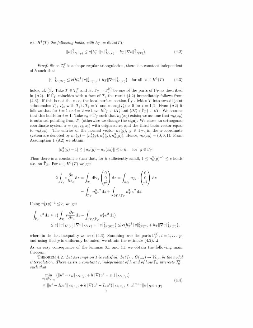
v ∈ H1(T ) the following holds, with hT := diam(T ):

‖v‖2L2(ΓT ) ≤ c(h−1T ‖v‖

2L2(T ) + hT ‖∇v‖2L2(T )

). (4.2)

Proof. Since T Γh is a shape regular triangulation, there is a constant independent

of h such that

‖v‖2L2(∂T ) ≤ c(h−1T ‖v‖

2L2(T ) + hT ‖∇v‖2L2(T )

)for all v ∈ H1(T ) (4.3)

holds, cf. [4]. Take T ∈ T Γh and let ΓT = Γ

(i)T be one of the parts of ΓT as described

in (A2). If ΓT coincides with a face of T , the result (4.2) immediately follows from(4.3). If this is not the case, the local surface section ΓT divides T into two disjointsubdomains T1, T2, with T1 ∪ T2 = T and meas3(Ti) > 0 for i = 1, 2. From (A2) itfollows that for i = 1 or i = 2 we have ∂ΓT ⊂ ∂Ti and (∂Ti \ ΓT ) ⊂ ∂T . We assumethat this holds for i = 1. Take x0 ∈ ΓT such that nh(x0) exists; we assume that nh(x0)is outward pointing from T1 (otherwise we change the sign). We chose an orthogonalcoordinate system z = (z1, z2, z3) with origin at x0 and the third basis vector equalto nh(x0). The entries of the normal vector nh(y), y ∈ ΓT , in the z-coordinatesystem are denoted by nh(y) = (n1

h(y), n2h(y), n3

h(y)). Hence, nh(x0) = (0, 0, 1). FromAssumption 1 (A2) we obtain

|n3h(y)− 1| ≤ ‖nh(y)− nh(x0)‖ ≤ c1h, for y ∈ ΓT .

Thus there is a constant c such that, for h sufficiently small, 1 ≤ n3h(y)−1 ≤ c holds

a.e. on ΓT . For v ∈ H1(T ) we get

2

∫T1

v∂v

∂z3dz =

∫T1

divz

00v2

dz =

∫∂T1

nT1·

00v2

dz

=

∫ΓT

n3hv

2 dz +

∫∂T1\ΓT

n3T1v2 dz.

Using n3h(y)−1 ≤ c, we get∫

ΓT

v2 dz ≤ c( ∫

T1

v∂v

∂z3dz −

∫∂T1\ΓT

n3T v

2 dz)

≤ c(‖v‖L2(T )‖∇v‖L2(T ) + ‖v‖2L2(∂T )

)≤ c(h−1T ‖v‖

2L2(T ) + hT ‖∇v‖2L2(T )

),

where in the last inequality we used (4.3). Summing over the parts Γ(i)T , i = 1, . . . , p,

and using that p is uniformly bounded, we obtain the estimate (4.2).

As an easy consequence of the lemmas 3.1 and 4.1 we obtain the following maintheorem.

Theorem 4.2. Let Assumption 1 be satisfied. Let Ih : C(ωh)→ Vh,m be the nodalinterpolation. There exists a constant c, independent of h and of how Γh interests T Γ

h ,such that

minvh∈V Γ

h,m

(‖ue − vh‖L2(Γh) + h‖∇(ue − vh)‖L2(Γh)

)≤ ‖ue − Ihue‖L2(Γh) + h‖∇(ue − Ihue)‖L2(Γh) ≤ chm+1‖u‖Hm+1(Γ)

(4.4)

7

for all u ∈ Hm+1(Γ) holds.Proof. From u ∈ Hm+1(Γ) it follows that ue ∈ Hm+1(ωh). Using Lemma 4.1 and

standard error bounds for the nodal interpolation Ih, we obtain, with vh := Ihue ∈

Vh,m:

‖ue − vh‖2L2(Γh) + h2‖∇(ue − vh)‖2L2(Γh)

=∑T∈T Γ

h

(‖ue − vh‖2L2(ΓT ) + h2‖∇(ue − vh)‖2L2(ΓT )

)≤ c

∑T∈T Γ

h

(h−1‖ue − vh‖2L2(T ) + h‖∇(ue − vh)‖2L2(T ) + h3‖∇2(ue − vh)‖2L2(T )

)≤ c

∑T∈T Γ

h

h2m+1‖ue‖2Hm+1(T ) = ch2m+1‖ue‖2Hm+1(ωh).

Using Assumption 1 (A1) and (3.8) with δ = c0h we get ‖ue‖2Hm+1(ωh) ≤ ch‖u‖2Hm+1(Γ),

which completes the proof.

From the result in this theorem we conclude that for the trace space V Γh,m we have

optimal approximation error bounds under (very) mild conditions on the approximatesurface Γh. If Γ and the exact solution u are sufficiently smooth, we obtain an hm+1

bound as in (4.4) (for finite elements of degree m), provided Assumption 1 is satisfied.The latter essentially only requires the accuracy dist(Γh,Γ) ≤ ch for the approximatesurface.

5. Finite element error bounds. In this section we prove optimal discretiza-tion error bounds both in the H1(Γh) and the L2(Γh) norm. For the discrete problem(2.5) such bounds for m = 1 (piecewise linear finite elements) are derived in [7].For the discrete problem (2.6) these error bounds for m = 1 are derived in [24]. Inboth references it is assumed that Γh is a piecewise planar approximation of Γ withdist(Γh,Γ) ≤ ch2. In this section we consider a more general setting with m ≥ 1 andmore general approximate surfaces Γh. Furthermore, we present the error analysisof the two discretizations in one unified setting, which reveals the main (theoretical)differences between the two methods.

In the analysis we need one further assumption, which quantifies the quality ofΓh as an approximation of Γ (“geometric error”).

Assumption 2. We assume that Γh ⊂ Uδ0 is a Lipschitz surface without bound-ary and that the projection p : Γh → Γ is a bijection. The corresponding unit normalfield is defined a.e. on Γh and denoted by nh. We assume that the following holds,for a k ≥ 1:

‖d‖L∞(Γh) ≤ chk+1, (5.1)

‖n− nh‖L∞(Γh) ≤ chk. (5.2)

These are the key assumptions we need in the analysis below. There is one furtherassumption we introduce. On each Γh there holds a Poincare inequality with a con-stant c = c(h). We assume that this constant is uniform w.r.t. h, i.e., we assume thatthere exists c, independent of h, such that

‖v‖L2(Γh) ≤ c‖∇Γhv‖L2(Γh) for all v ∈ H1(Γh)/R. (5.3)

8

Remark 2. We discuss cases in which the assumptions (5.1)-(5.2) are satisfied.Clearly, if Γh = Γ there is no geometric error, i.e. these assumptions are fulfilledwith k = ∞. Consider the case in which Γ is the zero level of a smooth level setfunction φ and φh is a finite element approximation of φ, on the triangulation Th.Let Γh be the zero level of φh. If ‖φ − φh‖L∞(ωh) + h‖∇(φ − φh)‖L∞(ωh) ≤ chk+1

holds, then the conditions (5.1)-(5.2) are satisfied. In [8] a method for constructingpolynomial approximations to Γ is presented that satisfies the conditions (5.1)-(5.2)(cf. Proposition 2.3 in [8]). In that method the exact distance function to Γ is needed.

We define the following projections

Ph(x) = I − nh(x)nh(x)T , Ph(x) = I − nh(x)n(x)T /(nh(x)Tn(x)), x ∈ Γh.

We collect a few results from [9]. The surface gradient of u ∈ H1(Γ) can be representedin terms of ∇Γhu

e as follows:

∇Γu(p(x)) =(I − d(x)H(x)

)−1Ph(x)∇Γhu

e(x) a.e. on Γh. (5.4)

For x ∈ Γh define

µh(x) = (1− d(x)κ1(x))(1− d(x)κ1(x))n(x)Tnh(x).

The integral transformation formula

µh(x)dsh(x) = ds(p(x)), x ∈ Γh, (5.5)

holds, where dsh(x) and ds(p(x)) are the surface measures on Γh and Γ, respectively.From ‖n(x)− nh(x)‖2 = 2

(1− n(x)Tnh(x)

), and Assumption 2 we obtain

‖1− µh‖L∞(Γh) ≤ chk+1, (5.6)

with a constant c independent of h. Using relation (5.4) and (5.5) we obtain∫Γ

∇Γu · ∇Γv ds =

∫Γh

Ah∇Γhue · ∇Γhv

e dsh for all u, v ∈ H1(Γ), (5.7)

with Ah(x) = µh(x)Ph(x)(I − d(x)H(x))−2Ph(x). (5.8)

We introduce a compact notation for the bilinear forms used in (2.5), (2.6):

ah(uh, vh) :=

∫Γh

∇uh · ∇vh dsh, aΓh(uh, vh) :=

∫Γh

∇Γhuh · ∇Γhvh dsh.

Furthermore, for the data error we introduce the notation

δf := fh − µhfe.

We now derive approximate Galerkin orthogonality relations for the discrete problems.Lemma 5.1. Let u be the solution of the Laplace-Beltrami equation (2.2) and

uh, uΓh ∈ V Γ

h,m the solutions of the discrete problems (2.5) and (2.6), respectively.

Define Ah := PhAhPh, with Ah as in (5.8). The following holds:

ah(ue − uh, vh) = Fh(vh) for all vh ∈ V Γh,m, (5.9)

with Fh(vh) :=

∫Γh

(I − Ah)∇ue · ∇vh dsh −∫

Γh

δfvh dsh.

aΓh(ue − uΓ

h, vh) = FΓh (vh) for all vh ∈ V Γ

h,m, (5.10)

with FΓh (vh) :=

∫Γh

(Ph − Ah)∇ue · ∇vh dsh −∫

Γh

δfvh dsh.

9

Proof. A function vh on Γh can be lifted on Γ by defining vlh(p(x)) := vh(x).From the definition of the discrete problem (2.5) and the transformation rule (5.7) weget

ah(uh, vh) =

∫Γh

fhvh dsh =

∫Γ

fvlh ds+

∫Γh

δfvh dsh

=

∫Γ

∇Γu · ∇Γvlh ds+

∫Γh

δfvh dsh =

∫Γh

Ah∇Γhue · ∇Γhvh ds+

∫Γh

δfvh dsh

=

∫Γh

Ah∇ue · ∇vh ds+

∫Γh

δfvh dsh,

where in the last inequality we used that ∇Γhvh = Ph∇vh. Combining this withah(ue, vh) =

∫Γh∇ue · ∇vh dsh we get the result in (5.9). Similar arguments can be

used to derive (5.10):

aΓh(uΓ

h, vh) =

∫Γh

∇ΓhuΓh · ∇Γhvh dsh =

∫Γ

fvlh ds+

∫Γh

δfvh dsh

=

∫Γh

Ah∇ue · ∇vh ds+

∫Γh

δfvh dsh.

We combine this with aΓh(ue, vh) =

∫ΓhPh∇ue · ∇vh dsh and thus get (5.10).

Note that the only difference between the perturbation terms Fh and FΓh in (5.9) and

(5.10) is in the matrices I − Ah and Ph − Ah. We derive bounds for the perturbationterms Fh and FΓ

h . We need some additional notation, namely H2(Γ)e := ve | v ∈H2(Γ) .

Lemma 5.2. Let Assumption 2 be fulfilled and assume that the data error satisfies‖δf‖L2(Γh) ≤ chk+s‖f‖L2(Γ) for an s ∈ [0, 1]. The following holds, with constants cindependent of h:

|Fh(v)| ≤ chk‖f‖L2(Γ)

(‖v‖L2(Γh) + ‖∇v‖L2(Γh)

)∀ v ∈ V Γ

h,m +H2(Γ)e, (5.11)

|FΓh (v)| ≤ chk+s‖f‖L2(Γ)

(‖v‖L2(Γh) + ‖∇Γhv‖L2(Γh)

)∀ v ∈ V Γ

h,m +H2(Γ)e, (5.12)

|Fh(ve)| ≤ chk+s‖f‖L2(Γ)

(‖v‖L2(Γ) + ‖∇Γv‖L2(Γ)

)∀ v ∈ H2(Γ). (5.13)

Proof. For the second term in Fh(v) and FΓh (v) we get

|∫

Γh

δfv dsh| ≤ ‖δf‖L2(Γh)‖v‖L2(Γh) ≤ chk+s‖f‖L2(Γ)‖v‖L2(Γh). (5.14)

Below we delete the argument x ∈ Γh in the notation. Using (3.4), P (p(x)) = P (x)and HP = PH we get

(I − Ah)∇ue = (I − Ah)P (I − dH)∇Γu(p(x)). (5.15)

We combine Ah = PhAhPh with the definition of Ah and with (5.1), (5.6), PhPh = Phand obtain

‖Ah − Ph‖L∞(Γh) ≤ chk+1. (5.16)

10

Hence, using (5.2) yields

‖(I − Ah)P‖L∞(Γh) ≤ ‖(I − Ph)P‖L∞(Γh) + chk+1

≤ ‖P − Ph‖L∞(Γh) + chk+1 ≤ chk.(5.17)

With the result in (5.15) we thus obtain∣∣ ∫Γh

(I − Ah)∇ue · ∇v dsh∣∣ ≤ chk‖∇Γu(p(·))‖L2(Γh)‖∇v‖L2(Γh)

≤ chk‖∇Γu‖L2(Γ)‖∇v‖L2(Γh) ≤ chk‖f‖L2(Γ)‖∇v‖L2(Γh),

(5.18)

and combining this with the result in (5.14) completes the proof of (5.11). In thedefinition of FΓ

h (v) we have the matrix Ph − Ah, instead of I − Ah. For the former

we have, cf. (5.16), ‖Ah − Ph‖L∞(Γh) ≤ chk+1. Furthermore we have

(Ph − Ah)∇ue · ∇v = Ph(Ph − Ah)∇ue · ∇v = (Ph − Ah)∇ue · ∇Γhv.

Similarly as in (5.18) we obtain∣∣ ∫Γh

(Ph − Ah)∇ue · ∇v dsh∣∣ ≤ chk+1‖∇Γu(p(·))‖L2(Γh)‖∇Γhv‖L2(Γh)

≤ chk+1‖f‖L2(Γ)‖∇Γhv‖L2(Γh),

and combining this with the result in (5.14) we get the bound (5.12). We finallyconsider the estimate (5.13). We use (3.4) and thus get, cf. (5.15),

(I − Ah)∇ue · ∇ve = [(I − dH)P (I − Ah)P (I − dH)]∇Γu(p(x)) · ∇Γv(p(x)).

For the matrix in the square brackets we have, cf. (5.16),

‖(I − dH)P (I − Ah)P (I − dH)‖L∞(Γh) ≤ ‖P (I − Ph)P‖L∞(Γh) + chk+1.

Using P (I − Ph)P = PnhnThP = (P − Ph)nhn

Th (P − Ph) and (5.2) we obtain

‖P (I − Ph)P‖L∞(Γh) ≤ ch2k. From this is follows that the norm of the matrix in

the square brackets is bounded by chk+1. Using similar arguments as in the deriva-tion of (5.12) above we then obtain the bound (5.13).

Remark 3. We comment on the data error ‖δf‖L2(Γh), with δf = fh − µhfe.For the choice fh = fe − 1

|Γh|∫

Γhfe dsh, which in practice often can not be realized,

we obtain, using (5.6), the data error bound ‖δf‖L2(Γh) ≤ chk+1‖f‖L2(Γ). Another,more feasible, possibility arises if we assume that f is a smooth function on Uδ0 . Asextension one can then use

fh(x) = f(x)− cf , cf :=1

|Γh|

∫Γh

f dsh.

Using∫

Γf ds = 0, (5.1), (5.6) and a Taylor expansion we get |cf | ≤ chk+1‖f‖H1

∞(Uδ0 )

and ‖f − µhfe‖L2(Γh) ≤ chk+1‖f‖H1∞(Uδ0 ). Hence, a data error bound ‖δf‖L2(Γh) ≤

chk+1‖f‖L2(Γ) with c = c(f) = c‖f‖H1∞(Uδ0 )‖f‖−1

L2(Γ) and a constant c independent of

f . Hence, in problems with smooth data it is realistic to assume that the condition onthe data error in Lemma 5.2 is satisfied with s = 1. In less regular situations, s < 1

11

may be more realistic.

Note that for s > 0 the bound on FΓh in (5.12) is of higher order in h than the one

for Fh in (5.11). This difference is reflected in the discretization error bounds derivedbelow. For Fh(ve) the higher order bound in (5.13) is obtained by using the specialstructure of ve (namely constant in normal direction). The latter bound is used inthe proof of the L2-error bound in Theorem 5.4 below.

Theorem 5.3. Let the Assumptions 1 and 2 be fulfilled. Assume that the dataerror satisfies ‖δf‖L2(Γh) ≤ chk+s‖f‖L2(Γ) for an s ∈ [0, 1]. Let uh and uΓ

h be thesolutions of the discrete problems (2.5) and (2.6), respectively. The following errorbounds hold, with a constant c independent of h and f :

‖∇(ue − uh)‖L2(Γh) ≤ c(hm‖u‖Hm+1(Γ) + hk‖f‖L2(Γ)

)(5.19)

‖∇Γh(ue − uΓh)‖L2(Γh) ≤ c

(hm‖u‖Hm+1(Γ) + hk+s‖f‖L2(Γ)

). (5.20)

Proof. Define eh := ue−uh and ψh := (Ihue)|Γh ∈ V Γ

h,m. We consider the splitting

‖∇eh‖2L2(Γh) = ah(eh, eh) = ah(eh, ue − ψh) + Fh(ψh − ue) + Fh(eh).

For the first two terms on the right-hand side we use (5.11) and the interpolationerror bounds of Theorem 4.2 and thus get

ah(eh, ue − ψh) + Fh(ψh − ue) ≤ c

(‖∇eh‖L2(Γh) + hk‖f‖L2(Γh)

)hm‖u‖Hm+1(Γ)

≤ 1

4‖∇eh‖2L2(Γh) + ch2m‖u‖2Hm+1(Γ) + ch2k‖f‖2L2(Γh). (5.21)

For the third term we need the Poincare inequality (5.3). Define cu =∫

Γhue dsh.

Using∫

Γuds = 0 and (5.6) we get |cu| ≤ chk+1‖u‖L2(Γ) ≤ chk+1‖f‖L2(Γ). Note that∫

Γheh − cu dsh = 0 holds, hence with the Poincare inequality we obtain

‖eh‖L2(Γh) ≤ ‖eh − cu‖L2(Γh) + chk+1‖f‖L2(Γ)

≤ c‖∇Γheh‖L2(Γh) + chk+1‖f‖L2(Γ) ≤ c‖∇eh‖L2(Γh) + chk+1‖f‖L2(Γ),

and using this in the estimate (5.11) yields

Fh(eh) ≤ chk‖f‖L2(Γ)

(‖∇eh‖L2(Γh) +hk+1‖f‖L2(Γ)

)≤ 1

4‖∇eh‖2L2(Γh) + ch2k‖f‖2L2(Γ).

Combining this with the result in (5.21) proves the bound in (5.19). The result in(5.20) follows with very similar arguments. Define eΓ

h = ue − uΓh, and consider the

splitting

‖∇ΓheΓh‖2L2(Γh) = aΓ

h(eΓh, e

Γh) = aΓ

h(eΓh, u

e − ψh) + FΓh (ψh − ue) + FΓ

h (eΓh).

Note that ‖∇Γh(ue − ψh)‖L2(Γh) ≤ ‖∇(ue − ψh)‖L2(Γh), hence for bounding the in-terpolation error we can use Theorem 4.2. We can repeat the arguments used above.Since in the bound for FΓ

h (v) in (5.12) we have a term hk+s (instead of hk) we getthe factor hk+s in the bound (5.20).

The result in this theorem yields optimal H1-error bounds for both methods, also forthe case of higher order finite elements (m ≥ 2). Of course, this optimal bound is

12

obtained only if the approximation error term, which is of order hm, is not dominatedby the geometric error term, which is of order hk and hk+s, respectively. Assumes = 1, cf. Remark 3. For the case k = m (which typically holds in case of linear finiteelements, i.e., m = 1), we see that for the method in (2.5) the geometric error is of thesame order as the approximation error, whereas for the method (2.6) the geometricerror is of higher order. For the method in (2.6) and m ≥ 2 we get the optimal orderof convergence hm even if we only have k = m− 1. The method (2.5) does not havethis property.

We apply a duality argument to obtain an L2(Γh)-error bound. In this analysisthe estimate (5.13) is used.

Theorem 5.4. Let the Assumptions 1 and 2 be fulfilled. Assume that the dataerror satisfies ‖δf‖L2(Γh) ≤ chk+s‖f‖L2(Γ) for an s ∈ [0, 1]. Let uh and uΓ

h be thesolutions of the discrete problems (2.5) and (2.6), respectively. The following errorbounds hold, with a constant c independent of h and f :

‖ue − uh‖L2(Γh) ≤ c(hm+1‖u‖Hm+1(Γ) + hk+s‖f‖L2(Γ)

)(5.22)

‖ue − uΓh‖L2(Γh) ≤ c

(hm+1‖u‖Hm+1(Γ) + hk+s‖f‖L2(Γ)

). (5.23)

Proof. Denote eh := ue−uh and let elh be the lift of eh|Γh on Γ and ce :=∫

Γelh ds.

Consider the problem: Find w ∈ H1(Γ) with∫

Γw ds = 0 such that∫

Γ

∇Γw · ∇Γv ds =

∫Γ

(elh − ce)v ds for all v ∈ H1(Γ). (5.24)

The solution w satisfies w ∈ H2(Γ) and ‖w‖H2(Γ) ≤ c‖elh‖L2(Γ)/R with ‖elh‖L2(Γ)/R :=

‖elh − ce‖L2(Γ). We take ψh = Ihwe ∈ Vh,m and with Ah = PhAhPh we obtain

‖elh‖2L2(Γ)/R =

∫Γ

∇Γw · ∇Γ(elh − ce) ds =

∫Γ

∇Γw∇Γelh ds

=

∫Γh

Ah∇Γheh · ∇Γhwe dsh =

∫Γh

∇eh · ∇we dsh +

∫Γh

∇eh · (Ah − I)∇we dsh

= ah(eh, we − ψh) + Fh(ψh − we) + Fh(we) +

∫Γh

∇eh · (Ah − I)∇we dsh. (5.25)

We consider the four terms in (5.25). Using the interpolation error bound in Theo-rem 4.2 (with m = 1), the error bound in Theorem 5.3 and ‖w‖H2(Γ) ≤ c‖elh‖L2(Γ)/Rwe get

ah(eh, we − ψh) ≤ c

(hm+1‖u‖Hm+1(Γ) + hk+1‖f‖L2(Γ)

)‖elh‖L2(Γ)/R.

For the second term we use (5.11) and the interpolation error bound (with m = 1),which yields

Fh(ψh − we) ≤ chk+1‖f‖L2(Γ)‖elh‖L2(Γ)/R.

For the third term we use (5.13) and get

Fh(we) ≤ chk+s‖f‖L2(Γ)‖w‖H1(Γ) ≤ chk+s‖f‖L2(Γ)‖elh‖L2(Γ)/R. (5.26)

13

For the last term we use (5.15) (with u replaced by w) and (5.17), which yields∫Γh

∇eh · (Ah − I)∇we dsh ≤ chk‖∇eh‖L2(Γh)‖∇Γw‖L2(Γ)

≤ c(hm+k‖u‖Hm+1(Γ) + h2k‖f‖L2(Γ)

)‖elh‖L2(Γ)/R.

Using these bounds in (5.25) yields

‖elh‖L2(Γ)/R ≤ c(hm+1‖u‖Hm+1(Γ) + hk+s‖f‖L2(Γ)

). (5.27)

Now note that

|ce| =∣∣ ∫

Γ

u− ulh ds∣∣ =

∣∣ ∫Γ

ulh ds∣∣ =

∣∣ ∫Γh

(µh − 1)uh dsh∣∣ ≤ chk+1‖f‖L2(Γ),

and thus

‖eh‖L2(Γh) ≤ c‖elh‖L2(Γ) ≤ c‖elh‖L2(Γ)/R + chk+1‖f‖L2(Γ),

and combining this with (5.27) completes the proof of (5.22). The result (5.23) canbe proved with very similar arguments. A proof of (5.23) for m = k = 1 is given in[24].

Note that the bounds in (5.22) and (5.23) are the same. We have an optimal errorif k + s ≥ m + 1 holds. If we have an optimal data approximation error, i.e. s = 1cf. Remark 3, we need k ≥ m to obtain an optimal L2-error bound of order hm+1.Inspection of the proof above shows that the factor hk+s in (5.22) originates (only)from the estimate (5.26). All other geometric error terms are of order hk+1. In theproof of (5.23) the term FΓ

h (we) has to be bounded. For this the estimate (5.12) isused. Inspection of the proof of the latter estimate reveals that the factor hk+s inthe bound in (5.12) can not be improved if we use the special choice v = we. Thus inboth error bounds, (5.22) and (5.23), we get the same geometric error term of orderhk+s.

6. Conditioning of the stiffness matrix. In this section we address linearalgebra aspects of the discretizations in (2.5) and (2.6). The discrete solution isdetermined by using the standard nodal basis of the (outer) finite element spaceVh,m. This nodal basis and the corresponding nodes are denoted by φi1≤i≤N andxi1≤i≤N , respectively. Hence, Vh,m = span (φi)|ωh | 1 ≤ i ≤ N , and dim(Vh,m) =N . By construction we have span (φi)|Γh | 1 ≤ i ≤ N = V Γ

h,m. Related to thelinear algebra, a key point is that in general the (φi)|Γh1≤i≤N are not independent,hence these do not form a basis of the trace space V Γ

h,m. This can be illustrated by

simple examples, cf. [23]. The representation vh =∑Ni=1 Viφi, vh ∈ Vh,m, induces the

isomorphism vh → V := (Vi)1≤i≤N ∈ RN . The vector corresponding to wh ∈ Vh,m isdeneoted by W . We introduce the mass and stiffness matrices:

〈MV,W 〉 =

∫Γh

vhwh dsh, for all vh, wh ∈ Vh,m, (6.1)

〈AV,W 〉 =

∫Γh

∇vh · ∇wh dsh, for all vh, wh ∈ Vh,m, (6.2)

〈AΓV,W 〉 =

∫Γh

∇Γhvh · ∇Γhwh dsh, for all vh, wh ∈ Vh,m. (6.3)

14

If (φi)|Γh1≤i≤N are dependent, there exists V ∈ RN , V 6= 0, such that vh =∑Ni=1 Viφi = 0 on Γh. This implies 〈MV,V 〉 = 0 and thus M is singular. Furthermore,

vh|Γh = 0 implies (∇Γhvh)|Γh = 0 and thus 〈AΓV, V 〉 = 0, hence AΓ is singular. Thisindicates that the conditioning properties of the mass matrix M and the stiffnessmatrix AΓ are different from that of standard finite element discretizations of ellipticproblems. In [23] this conditioning issue is studied. We outline a few importantresults. In numerical experiments it is observed that for the Laplace-Beltrami equationdiscretized with linear trace finite elements on an approximate surface Γh that isobtained as the zero level of a piecewise linear level set function the mass matrixM has one zero eigenvalue (within machine accuracy) and the stiffness matrix AΓ

has two zero eigenvalues. The effective condition number is defined as the quotientof the largest and the smallest nonzero eigenvalue. Typically both the diagonallyscaled mass matrix D−1

M M and the diagonally scaled stiffness matrix D−1AΓAΓ have

effective condition numbers that behave like h−2. In [23] a rather technical analysis ispresented that gives a theoretical explanation of these conditioning properties. Theanalysis is only for the two-dimensional case (i.e., Γ is a curve) and uses technicalassumptions related to how Γh intersects the local triangulation T Γ

h . An exampleof such an assumption is that the relative size of the set of vertices in T Γ

h having acertain maximal distance to Γh gets smaller if this distance gets smaller (for precisestatements we refer to [23]). In the recent paper [5] a stabilization technique for (2.6)is introduced, which improves the conditioning properties of AΓ.

The discretization (2.5) is more stable than (2.6) in the sense that ‖∇vh‖L2(Γh) ≥‖∇Γhvh‖L2(Γh) holds. Related to this, note that vh|Γh = 0 does not necessarily implythat (∇vh)|Γh = 0 holds. Based on this, one might expect a better conditioning ofthe matrix A compared to AΓ. This is indeed observed in numerical experiments,cf. section 7. In this section we derive conditioning properties of the stiffness matrixA for the case m = 1, i.e., linear finite elements. Using an elementary analysis itis shown that a suitably scaled A has a condition number that behaves like h−2 (onthe space orthogonal to the constant), independent of how Γh intersects T Γ

h . Such arobustness property w.r.t. the geometry does not hold for the scaled stiffness matrixAΓ. As a simple corollary we obtain a conditioning result for a shifted mass matrix,cf. Theorem 6.3.

We consider m = 1 and use the notation Vh := Vh,1. In Remark 4 we comment onm ≥ 2. For a node xi, let T (xi) be the set of all tetrahedra T ∈ T Γ

h that contain xi.Define

δT :=|ΓT ||T |

h, T ∈ T Γh , di :=

∑T∈T (xi)

δT , 1 ≤ i ≤ N.

(Recall: ΓT = Γh ∩ T ). We introduce a weighted L2(ωh)-norm:

‖v‖2δ,ωh =∑T∈T Γ

h

δT

∫T

v2 dx,

and a related scaled vector norm:

‖V ‖2D := 〈DV, V 〉, D := diag(di).

From the fact that ∇φi · ∇φi is constant on each T ∈ T (xi) with value ∼ h−2 itfollows that D is uniformly spectrally equivalent to diag(A). Hence, the scaling with

15

D that is used below, can be replaced by a scaling with diag(A). The constants usedin the lemma and theorems below are independent of h and of how Γh intersects thelocal triangulation T Γ

h .Lemma 6.1. There are constants c1 > 0 and c2 such that

c1h3‖V ‖2D ≤ ‖vh‖2δ,ωh ≤ c2h

3‖V ‖2D for all vh ∈ Vh.

Proof. We use the compact notation ∼ to represent inequalities in both directionswith constants independent of h and of how Γh intersects Ωh. The set of vertices ofT is denoted by V(T ). For vh ∈ Vh we have Vi = vh(xi) and∫

T

v2h dx ∼ |T |

∑xi∈V(T )

vh(xi)2 ∼ h3

∑xi∈V(T )

V 2i .

This implies

‖vh‖2δ,ωh =∑T∈T Γ

h

δT

∫T

v2h dx ∼ h3

∑T∈T Γ

h

δT∑

xi∈V(T )

V 2i

= h3N∑i=1

( ∑T∈T (xi)

δT)V 2i = h3

N∑i=1

diV2i = h3‖V ‖2D,

and thus the result holds.

Theorem 6.2. There are constants c1 > 0 and c2 such that

c1h2‖V ‖2D ≤ 〈AV, V 〉 ≤ c2‖V ‖2D for all V ∈ RN with

∫Γh

vh ds = 0.

Proof. We first consider the upper bound. Note that, using an inverse inequalityon T we get:

〈AV, V 〉 =

∫Γh

∇vh · ∇vh ds ≤∑T∈T Γ

h

|ΓT | ‖∇vh‖2L∞(T ) ≤ c∑T∈T Γ

h

h−2 |ΓT ||T |‖vh‖2L2(T )

= ch−3∑T∈T Γ

h

δT

∫T

v2h dx = ch−3‖vh‖2δ,ωh ≤ c‖V ‖

2D,

where in the last inequality we used Lemma 6.1.We now consider the lower bound. Using Lemma 6.1 we get

h2‖V ‖2D ≤ ch−1‖vh‖2δ,ωh = ch−1∑T∈T Γ

h

δT

∫T

v2h dx. (6.4)

Take a T ∈ T Γh . Let ξ ∈ T, η ∈ ΓT be such that |vh(x)| ≤ |vh(ξ)| for all x ∈ T and

|vh(η)| ≤ |vh(x)| for all x ∈ ΓT . From vh(ξ) = vh(η) + (ξ − η) · ∇vh|T it follows that|vh(ξ)|2 ≤ c(|vh(η)|2 + h2‖∇vh|T ‖2). Using this we obtain

h−1δT

∫T

v2h dx ≤ |ΓT ||vh(ξ)|2 ≤ c

(|ΓT ||vh(η)|2 + |ΓT |h2‖∇vh|T ‖2

)≤ c( ∫

ΓT

v2h ds+ h2

∫ΓT

‖∇vh‖2 ds.)

16

Summing over T ∈ T Γh and using the Poincare inequality (5.3) (which holds for vh

with∫

Γhvh dsh = 0), we get

h−1∑T∈T Γ

h

δT

∫T

v2h dx ≤ c

( ∫Γh

v2h ds+ h2

∫Γh

‖∇vh‖2 ds)

(6.5)

≤ c( ∫

Γh

‖∇Γhvh‖2 ds+ h2

∫Γh

‖∇vh‖2 ds)≤ c

∫Γh

‖∇vh‖2 ds = c〈AV, V 〉.

Combining this with the result in (6.4) completes the proof.

As an immediate conseqence of this theorem we obtain for the spectral conditionnumber in the space orthogonal to the one dimensional kernel (corresponding to theconstant fuction), denoted by κ∗(·):

κ∗(D−1A) ≤ ch−2. (6.6)

We derive a result for a shifted mass matrix.Theorem 6.3. There are constants c1, c2 > 0 such that for all α ≥ 0:

c1(min2h2, α+ αh2)‖V ‖2D ≤ 〈MV,V 〉+ α〈AV, V 〉 ≤ c2(h2 + α)‖V ‖2D,

for all V ∈ RN with∫

Γhvh ds = 0.

Proof. First we consider the upper bound. Note that

〈MV,V 〉 =

∫Γh

v2h ds ≤

∑T∈T Γ

h

|ΓT |‖vh‖2L∞(T ) ≤ ch−1

∑T∈T Γ

h

δT

∫T

v2h ds

= ch−1‖vh‖2δ,ωh ≤ ch2‖V ‖2D.

In combination with Theorem 6.2 this yields the upper bound. For the lower boundwe use the result in (6.5) and in Lemma 6.1 and thus get:

〈MV,V 〉+h2〈AV, V 〉 =

∫Γh

v2h ds+h2

∫Γh

‖∇vh‖2 ds ≥ ch−1‖vh‖2δ,ωh ≥ c0h2〈DV, V 〉,

with a constant c0 > 0. Using spectral inequalities for symmetric positive matriceswe have: M + h2A ≥ c0h2D. From this and the lower bound in Theorem 6.2 we get

M + αA = M +( α

2h2

)h2A+

1

2αA ≥ min1, α

2h2(M + h2A

)+

1

2αA

≥ c0 min1, α

2h2h2D + c1αh

2D ≥ c(

min2h2, α+ αh2)D,

which proves the lower bound.

Thus we have the following bound for the spectral condition number:

κ∗(D−1(M + αA)

)≤ c h2 + α

min2h2, α+ αh2. (6.7)

For α→∞ we get the same bound as in (6.6). For α ↓ 0 the bound tends to infinity.This can not be avoided, since the mass matrix M can be singular (also in the spaceorthogonal to the constant), as explained above. More interesting is the case α ≥ ch2

with c > 0. Then the bound takes the form ch−2 α1+α . Hence, if α ∼ h2 we get a

17

uniform (i.e. independent of h) condition number bound and if α ∼ h we get a boundof the form ch−1. The case α ∼ h2 is typical if a time dependent surface diffusionproblem is considered in which for the time discretization an implicit Euler methodis used with ∆t ∼ h2. If for such a time dependent problem one uses Crank-Nicolsonwith ∆t ∼ h, this results in a linear system with α ∼ h.

Remark 4. We comment on the case of higher order finite elements, i.e. m ≥ 2.Inspection of the proofs, shows that the estimates in Lemma 6.1 and the upper boundin Theorem 6.2 also hold if m ≥ 2 is considered. The lower bound in Theorem 6.2,however, does not hold in general. This becomes clear from the following exam-ple. Consider a two-dimensional setting with a domain ω = [0, 1] × [−1, 1] which issubdivided into a few triangles with vertices only on y = −1 or y = 1. We takeΓh = [0, 1] × 0. We choose the P2 finite element function v(x, y) = αy2 + (x − 1

2 )with α 1. For this function we have ‖v‖L2(ω) ∼ α,

∫Γhv ds = 0, ∇v = (1, 2αy)T

and thus ‖∇v‖L2(Γh) = 1. The lower bound in Theorem 6.2 scales with ‖v‖2L2(ω) ∼ α2,

whereas 〈AV, V 〉 = ‖∇v‖2L2(Γh) = 1 holds. Hence, we conclude that the first inequalityin Theorem ?? can not hold for this simple example. The key point in this exampleis that we can not control the values of vh on ω by its values and gradient on Γh.

7. Numerical experiments. In this section we present results of a numericalexperiment. As a test problem we consider the Laplace-Beltrami equation on the unitsphere:

−∆Γu = f on Γ,

with Γ = x ∈ R3 | ‖x‖2 = 1 and Ω = (−2, 2)3.The source term f is taken such that the solution is given by

u(x) =1

‖x‖3(3x2

1x2 − x32

), x = (x1, x2, x3) ∈ Ω.

Using the representation of u in spherical coordinates one can verify that u is aneigenfunction of −∆Γ:

u(r, φ, θ) = sin(3φ) sin3 θ, −∆Γu = 12u =: f(r, φ, θ). (7.1)

The right-hand side f satisfies the compatibility condition∫

Γf ds = 0, likewise does

u. Note that u and f are constant along normals at Γ.A family Tll≥0 of tetrahedral triangulations of Ω is constructed as follows. We

triangulate Ω by starting with a uniform subdivision into 48 tetrahedra with mesh sizeh0 =

√3. Then we apply an adaptive red-green refinement-algorithm (implemented

in the software package DROPS [11]) in which in each refinement step the tetrahedrathat contain Γ are refined such that on level l = 1, 2, . . . we have

hT ≤√

3 2−l =: hl for all T ∈ Tl with T ∩ Γ 6= ∅.

The family Tll≥0 is consistent and shape-regular. The interface Γ is the zero-levelof ϕ(x) := ‖x‖2 − 1. Let ϕh := Ih(ϕ) where Ih is the standard nodal interpolationoperator on Tl. The discrete interface is given by Γhl := x ∈ Ω | I(φh)(x) = 0 .This discrete interface triangulation is very shape-irregular. For the extension fh of fwe take the constant extension of f along the normals at Γ, i.e. we take fh(r, φ, θ) =f(1, φ, θ) + ch, with f(r, φ, θ) as in (7.1) and ch such that

∫Γhfh dsh = 0. For the

18

computation of the integrals∫Tfhφh dsh we use a quadrature-rule that is exact up to

order five.We consider the discrete problems (2.5) and (2.6) with solutions uh and uΓ

h,respectively.

The discretization errors in the L2(Γh)-norm are given in table 7.1. The extensionue of u is given by ue(r, φ, θ) := u(1, φ, θ) = u(r, φ, θ) (since u is constant along nΓ).

level l ‖ue − uh‖L2(Γh) factor ‖ue − uΓh‖L2(Γh) factor

1 0.6276 – 0.4418 –2 0.1983 3.16 0.1149 3.853 0.05299 3.74 0.02965 3.874 0.01348 3.93 0.007298 4.065 0.003387 3.98 0.001865 3.916 0.0008476 4.00 0.0004629 4.037 0.0002120 4.00 0.0001158 4.00

Table 7.1Discretization errors and error reduction.

These results clearly show the h2 behaviour as predicted by the analysis. We alsoobserve that the discretization error for uΓ

h is about a factor two smaller than for uh.

We now consider the conditioning of the stiffness matrices and shifted mass matrix.The matrices M,A,AΓ and D are as defined in section 6. Define DAΓ

:= diag(AΓ)and the scaled matrices

A := D−12AD−

12 , AΓ := D

− 12

AΓAΓD

− 12

AΓ, Mα := D−

12

(M + αA)D−

12 .

The discrete problems are solved using a standard CG method with symmetric SORpreconditioner applied to the discrete problems with stiffness matrices A and AΓ. Weuse a relative tolerance of 10−6. In the tables below m gives the number of unknows(dimension of the matrices). In the tables 7.2 and 7.3 “# iter” gives the numberof preconditioned CG iterations needed to solve the system (with accuracy 10−6).Furthermore, for different refinement levels we computed the largest and smallesteigenvalues of scaled the matrices.

level l m factor λ1 λ2 λm λm/λ2 factor # iter

1 100 - 0 0.021 0.51 24.0 - 112 448 4.48 0 0.0053 0.52 98.9 4.1 183 1864 4.16 0 0.0013 0.54 412 4.2 334 7552 4.05 0 0.00033 0.54 1667 4.0 59

Table 7.2Conditioning of scaled stiffness matrix A

We observe that, as predicted by the theory, the effective condition number forA behaves like ∼ h−2 and that this condition number is smaller the one of AΓ. Thebetter conditioning of A is also reflected in the results for # iter. Also note that Ahas only one zero eigenvalue (corresponding to the constant function), whereas AΓ

19

level l m factor λ1 λ2 λ3 λm λm/λ3 factor # iter

1 100 - 0 0 0.055 2.16 39.2 - 132 448 4.48 0 0 0.014 2.19 154 3.9 253 1864 4.16 0 0 0.0033 2.34 710 4.6 494 7552 4.05 0 0 0.00077 2.43 3150 4.4 98

Table 7.3Conditioning of scaled stiffness matrix AΓ

has two zero eigenvalues. In Table 7.4 we present results for the spectral conditionnumber κ∗(Mα) for the cases α = h2

l and α = hl. The results are in very goodagreement with the bound derived in (6.7).

level l m κ∗(Mα), α = h2l κ∗(Mα), α = hl

1 100 12.7 25.02 448 13.1 50.73 1864 13.5 1044 7552 13.6 209

Table 7.4Conditioning of scaled shifted mass matrix Mα

REFERENCES

[1] D. Adalsteinsson and J. A. Sethian, Transport and diffusion of material quantities onpropagating interfaces via level set methods, J. Comput. Phys., 185 (2003), pp. 271–288.

[2] B. Alberta, A. Johnson, J. Lewis, M. Raff, K. Roberts, and P. Walter, MolecularBiology of the Cell, Garland Science, New York, fouth ed., 2002.

[3] D. Braess, Finite Elements: Theory, Fast Solvers, and Applications in Solid Mechanics, 3dedition, Cambridge University Press, 2007.

[4] L. Brenner, S.and Scott, The Mathematical Theory of Finite Element Methods, Springer,New York, second ed., 2002.

[5] E. Burman, P. Hansbo, and M. Larson, A stable cut finite element method for partial dif-ferential equations on surfaces: The Laplace-Beltrami operator, preprint, arXiv:1312.1097,2013.

[6] A. Chernyshenko and M. Olshanskii, Non-degenerate Eulerian finite element method forsolving PDEs on surfaces, Rus. J. Num. Anal. Math. Model., 28 (2013), pp. 101–124.

[7] K. Deckelnick, C. Elliott, and T. Ranner, Unfitted finite element methods using bulkmeshes for surface partial differential equations, preprint, arXiv:1312.2905, 2013.

[8] A. Demlow, Higher-order finite element methods and pointwise error estimates for ellipticproblems on surfaces, SIAM J. Numer. Anal., 47 (2009), pp. 805–827.

[9] A. Demlow and G. Dziuk, An adaptive finite element method for the Laplace-Beltrami oper-ator on implicitly defined surfaces, SIAM J. Numer. Anal., 45 (2007), pp. 421–442.

[10] A. Demlow and M. Olshanskii, An adaptive surface finite element method based on volumemeshes, SIAM J. Numer. Anal., 50 (2012), pp. 1624–1647.

[11] DROPS package. http://www.igpm.rwth-aachen.de/DROPS/.[12] G. Dziuk, Finite elements for the beltrami operator on arbitrary surfaces, in Partial differential

equations and calculus of variations, S. Hildebrandt and R. Leis, eds., vol. 1357 of LectureNotes in Mathematics, Springer, 1988, pp. 142–155.

[13] G. Dziuk and C. Elliott, Finite elements on evolving surfaces, IMA J. Numer. Anal., 27(2007), pp. 262–292.

[14] , An Eulerian approach to transport and diffusion on evolving implicit surfaces, ComputVisual Sci, 13 (2010), pp. 17–28.

20

[15] C. M. Elliott, B. Stinner, V. Styles, and R. Welford, Numerical computation of ad-vection and diffusion on evolving diffuse interfaces, IMA J. Numer. Anal., 31 (2011),pp. 786–812.

[16] J. B. Greer, An improvement of a recent Eulerian method for solving PDEs on general ge-ometries, J. Sci. Comput., 29 (2008), pp. 321–352.

[17] S. Groß and A. Reusken, Numerical Methods for Two-phase Incompressible Flows, Springer,Berlin, 2011.

[18] A. Hansbo and P. Hansbo, An unfitted finite element method, based on nitsche’s method, forelliptic interface problems, Comput. Methods Appl. Mech. Engrg., 191 (2002), pp. 5537–5552.

[19] , A finite element method for the simulation of strong and weak discontinuities in solidmechanics, Comput. Methods Appl. Mech. Engrg., 193 (2004), pp. 3523–3540.

[20] M. Olshanskii and A. Reusken, Error analysis of a space-time finite element method forsolving PDEs on evolving surfaces, IGPM Preprint No 376, Department of Mathematics,RWTH Aachen University. Revised version submitted to SIAM J. Numer. Anal., (2013).

[21] M. Olshanskii, A. Reusken, and X. Xu, An Eulerian space-time finite element method fordiffusion problems on evolving surfaces, NA&SC Preprint No 5, Department of Mathemat-ics, University of Houston. Revised version submitted to SIAM J. Numer. Anal., (2013).

[22] , A stabilized finite element method for advection-diffusion equations on surfaces, IMAJ. of Numer. Anal., doi:10.1093/imanum/drt016, (2013).

[23] M. A. Olshanskii and A. Reusken, A finite element method for surface PDEs: Matrix prop-erties, Numer. Math., 114 (2010), pp. 491–520.

[24] M. A. Olshanskii, A. Reusken, and J. Grande, A finite element method for elliptic equationson surfaces, SIAM J. Numer. Anal., 47 (2009), pp. 3339–3358.

[25] T. Ranner, Computational surface partial differential equations, PhD thesis, University ofWarwick, 2013.

[26] J. A. Sethian, Theory, algorithms, and applications of level set methods for propagating in-terfaces, Acta Numerica, 5 (1996), pp. 309–395.

[27] J.-J. Xu and H.-K. Zhao, An Eulerian formulation for solving partial differential equationsalong a moving interface, Journal of Scientific Computing, 19 (2003), pp. 573–594.

21