6th

International Conference on Advances in Experimental Structural Engineering

11th

International Workshop on Advanced Smart Materials and Smart Structures Technology

August 1-2, 2015, University of Illinois, Urbana-Champaign, United States

Analysis of Time-Frequency Energy for Environmental Vibration

Induced by Metro

Guangzhen Li1, Xiaosong Ren2

, Bin Zhang3 ,Gang Zong4

1 Graduate student, Research Institute of Structural Engineering and Disaster Reduction, Tongji University, Shanghai

200092, China.

E-mail: 1332857@tongji.edu.cn

2 Professor, Research Institute of Structural Engineering and Disaster Reduction, Tongji University, Shanghai 200092,

China.

E-mail: rxs@tongji.edu.cn

3 Graduate student, Research Institute of Structural Engineering and Disaster Reduction, Tongji University, Shanghai

200092, China.

E-mail: 972373707@qq.com

4 Lecturer, Research Institute of Structural Engineering and Disaster Reduction, State Key Laboratory of Disaster

Reduction in Civil Engineering, Tongji University, Shanghai 200092, China.

E-mail: zong@tongji.edu.cn

ABSTRACT

Time and frequency domain analysis processing are two conventional methods for vibration analysis. Despite

the advantages in the time or frequency domain, the cluttering of non-stationery signal cannot be effectively

distinguished by time domain analysis, and the characteristics in certain frequency segments may be neglected

in the frequency domain analysis.

By the adjustment of the length of time window, time-frequency energy method can effectively show the

characteristics of energy in time domain and do the component analysis in the specific frequency range. Hence

the local characteristics of signals in the useful range can be got. Although this method was put forward early, it

is not widely used for the restriction of the hardware and software for numerical analysis.

The ground vibration induced by metro is neither a kind of stationary vibration nor a transient impact vibration.

The energy is concentrated in the frequency range above 50Hz. This paper presents the signal processing using

time-frequency energy method. The signals collected in 8 points along the direction vertical to the metro line are

chosen as examples. By comparative study of signal duration, frequency band recognition and energy

characterization, the vibration signal induced by non-metro aspects can effectively be separated and the

propagation law for metro-induced vibration can be found.

KEYWORDS: Time-frequency energy; Environmental vibration induced by metro, Signal analysis processing,

Local characteristic

Signal analysis processing is usually done in time domain and frequency domain. From the analysis in time

domain, the characteristics, such as time duration, the peak value, the RMS (root-mean-square) and the

attenuation curve can be easily got, and the cross-correlation function can reveal the linear dependence between

different signals. On the other hand, the signal analysis in frequency domain can proceed by using the Fourier

Transform. The frequency components can be got and hence modal identification can be done by the

combination of auto-power spectrum and cross-power spectrum.

For non-stationary signals, time history analysis and frequency spectrum analysis seem not effective and

convincible. For example, the RMS as an energy representation is a mean value along time axis which may not

reflect the reality for the reason of determination of duration for weak signal, while Fourier Transform is also

not accurate enough for analyzing local characteristic of the non-stationary signal.

In the 40s of last century, the concept of time-frequency energy was put forward for the treatment of the

non-stationary signals. Compared with the traditional processing method, time-frequency energy shows

advantage in analyzing local characteristic of frequency domain because the length of time-window and

frequency-window can be adjusted to get a balance of accuracy between time domain and frequency domain.

The time-frequency energy is the direct reflection of signal energy and makes the energy characterization more

close to the reality, which overcomes the scattering of signal energy by using traditional method. The references

as [1-5] show that so far the signal processing is still separated in time domain or frequency domain. The main

reason is the restriction of the hardware and software for numerical application of time-frequency energy.

As a typical environmental vibration signal with evident local characteristics, the metro-induced ground

vibration is neither a kind of stationary vibration nor a transient impact vibration. Due to the relative gradual

variety of envelope in the whole process of signal, the time domain analysis is still suitable for signal evaluation.

While from the view on signal detail, it is more like a transient impact vibration signal and the parameters in

time domain, such as the peak value, RMS, vibration acceleration level by weighted RMS cannot accurately

describe the characteristics of signal. In this paper, the ground vibration induced by metro is analyzed by the

means of time-frequency energy and through the comparison to the traditional method, the advantages of

time-frequency energy is presented.

1. INTRODUCTION OF TIME-FREQUENCY ENERGY

For the signal x t , the frequency representation can be obtained by the Fourier transform,

2j ftX f x t e dt

(1.1)

where f is the signal frequency .The energy xE can be calculated through the integral as follows.

2 2( ) ( )xE x t dt X f d f

(1.2)

where 2

( )x t and 2

( )X f are used as the representation of energy in time domain and frequency domain.

Similarly, quadratic time-frequency distribution is used for the instantaneous signal energy in this paper,

Among the classic quadratic time-frequency distribution functions, the Cohen bilinear time-frequency

distribution function and Affine bilinear time-frequency distribution function are most commonly used for

expression of time-frequency transform [6]. As the real part of Rihaczek time-frequency distribution, which is

one kind of Cohen bilinear time-frequency distribution, Margenau-Hill-Spectrogram distribution is different

from other time-frequency distribution for dealing with signal energy. It is the direct description of the discrete

signal energy and has advantages to treat the cross-term, minus energy and edge effect optimization [7]. In this

paper, the time-frequency energy analysis is based on Margenau-Hill-Spectrogram distribution. The

time-frequency distribution is defined as follows.

*1( , ) ( , ; ) ( , ; )x x x

gh

MHS t f R F t f h F t f gK

(1.3)

where ( , )xMHS t f is the time-frequency distribution coefficient; R represents the real part of an imaginary

number; ( , ; )x

F t f h is Rihaczek distribution in time domain with window g ; *( , ; )x

F t f g

is conjugate of Rihaczek

distribution in frequency domain with window h ;*( ) ( )ghK h u g u du

is the integration for time window h

and conjugate of frequency window g , which is used to adjust the additive energy caused by the window.

The instantaneous frequency estimation, group delay estimation, effective duration (abbreviated as TE) and

effective frequency band (abbreviated as BF) and so on, are used as evaluation index of time-frequency

characteristics, as stated in Ref. [8-10]. The instantaneous frequency estimation is to describe the instantaneous

frequency feature on the local time point, while the instantaneous frequency on the whole duration reflects the

time-dependent law of frequency. The group delay demonstrates the phase rate of changes due to the frequency

change rate, which is intuitively time delay of signal waveform envelope. The effective duration and the

effective frequency band are two parameters to show the duration range and frequency band that contribute most

to the signal energy. The effective duration is used to calculate the concentration degree of the signal and the

effective frequency band is used to calculate the bandwidth of the signal frequency [10].

2 2

2 ( )m

x

TE t t x t dtE

(1.4)

2 2

2 ( )m

x

BF f f X f dfE

(1.5)

where mt and mf are the time center and frequency center, respectively.

21( )m

x

t t x t dtE

(1.6)

21( )m

x

f f X f dvE

(1.7)

The signal can be characterized in the time-frequency plane by its center position ( , )m mt f and a domain of

time-bandwidth product as TE BF .

The energy value can be calculated in any time and frequency range for concern. Here, the energy value is

calculated just in the effective duration and effective frequency band. This kind of calculation eliminates the

problem of scattering of signal energy over duration and the influence of other frequency.

The local energy E can be calculated through the integral of time-frequency distribution coefficient as follows.

( , )m m

m m

t t f f

t t f fE P t f dtdf

(1.8)

where ( , )P t f is the time-frequency distribution coefficient, the same as Eq. (1.3) in this paper; 2

TEt

2

BFf .

For the discrete signal, the formula can be expressed as follows.

( , )i i

i i i

t v

E P t v (1.9)

where ( , )i i iP t v is the discretized value of time-frequency distribution ( , )P t f at position ( , )i it f .

It is seen that the time-frequency energy can be used for the analysis of energy distribution of the transient

impact signal in the concerned time length and frequency range.

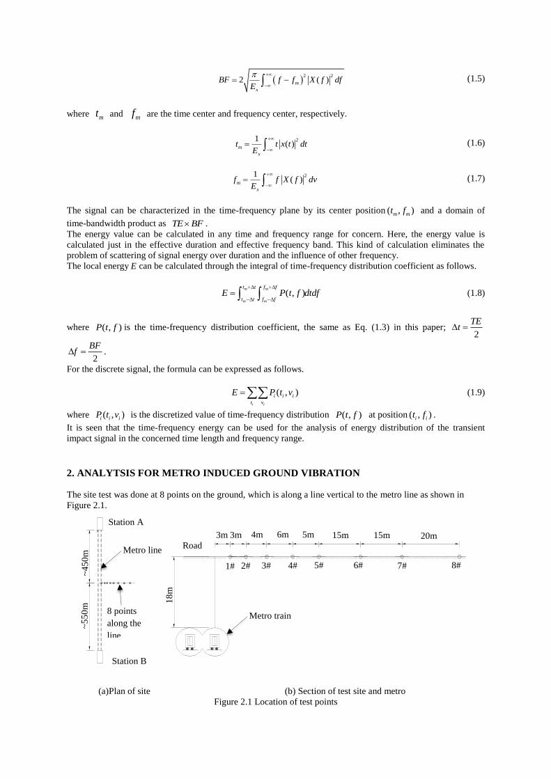
2. ANALYTSIS FOR METRO INDUCED GROUND VIBRATION

The site test was done at 8 points on the ground, which is along a line vertical to the metro line as shown in

Figure 2.1.

(a)Plan of site (b) Section of test site and metro

Figure 2.1 Location of test points

Station A

Station B

~4

50

m

~5

50

m

8 points

along the

line

1#

#

1

4# 2# 3# 5# 6# 7# 8#

3m 3m 4m 6m 5m 15m 15m 20m

18

m

Metro line

Metro train

Road

d

The test points are located in one side of the metro line as it is an empty construction site, and many buildings

are at the opposite side of these test points. The metro line is beneath the road with depth of about 18 meters.

The total length of site test is 4 fours in the morning. The distance between two metro stations is about 1km and

the test points are nearly located in the middle. Although the metro is moving on two ways, the test points are

mainly influenced by the metro train of the near side in one way.

As the metro is passing away about every 2 minutes, the signals including the metro and non-metro aspects are

measured. The time duration for metro influence is found to be about 15 seconds. In order to get the influence of

metro on the ground vibration, it is necessary to distinguish the signals induced by the metro and non-metro

aspects.

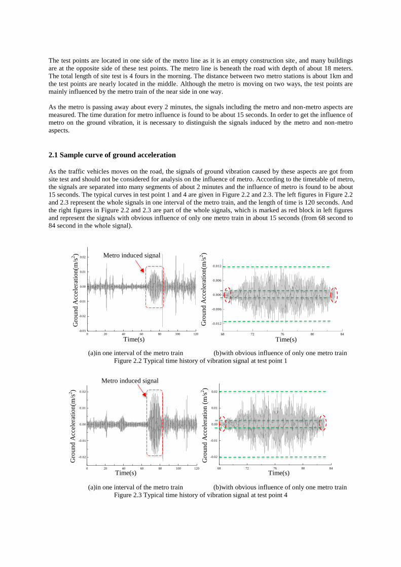
2.1 Sample curve of ground acceleration

As the traffic vehicles moves on the road, the signals of ground vibration caused by these aspects are got from

site test and should not be considered for analysis on the influence of metro. According to the timetable of metro,

the signals are separated into many segments of about 2 minutes and the influence of metro is found to be about

15 seconds. The typical curves in test point 1 and 4 are given in Figure 2.2 and 2.3. The left figures in Figure 2.2

and 2.3 represent the whole signals in one interval of the metro train, and the length of time is 120 seconds. And

the right figures in Figure 2.2 and 2.3 are part of the whole signals, which is marked as red block in left figures

and represent the signals with obvious influence of only one metro train in about 15 seconds (from 68 second to

84 second in the whole signal).

0 20 40 60 80 100 120

-0.03

-0.02

-0.01

0.00

0.01

0.02

68 72 76 80 84

-0.012

-0.006

0.000

0.006

0.012

(a)in one interval of the metro train (b)with obvious influence of only one metro train

Figure 2.2 Typical time history of vibration signal at test point 1

0 20 40 60 80 100 120

-0.02

-0.01

0.00

0.01

0.02

68 72 76 80 84

-0.02

-0.01

0.00

0.01

0.02

(a)in one interval of the metro train (b)with obvious influence of only one metro train

Figure 2.3 Typical time history of vibration signal at test point 4

Time(s) Time(s)

Gro

un

d A

ccel

erat

ion

(m/s

2)

Gro

un

d A

ccel

erat

ion

(m/s

2)

Metro induced signal

Gro

un

d A

ccel

erat

ion

(m/s

2)

Gro

un

d A

ccel

erat

ion

(m

/s2)

Time(s)

Metro induced signal

Time(s)

10 sample curves with duration of about 15 seconds are chosen for analysis in this paper. The typical curves

involve a short period of the ground-borne vibration with peak value as 0.002m/s2 at the beginning and the end

of the signal, which are marked by red dashed circles in the graph. From the site test in other quiet periods, the

typical curves of the ground borne vibration is found with peak value as 0.002 m/s2, which is consistent with the

test signals at the beginning and the end.

It can be found that the peak acceleration in test point 1 and 4 are about 0.012 m/s2 and 0.020 m/s

2, which

includes the influence of the ground borne vibration. Although the ground borne vibration cannot be eliminated

directly by subtracting it from the test signals, the peak value of ground vibration at test point 4 is much larger

than that at test point 1. It is an interesting phenomenon of metro-induced ground vibration and will be

demonstrated by other methods later.

2.2 Analysis by traditional method

The average value of the ten signal duration turns to be 15.91 seconds, as shown in Table 2.1. For the reason of

not restrict way for truncating data from the whole record, the time duration of signal may be shorter or longer

when the ground borne vibration is less or more considered for analysis.

Table 2.1 Statistic value of metro vibration signal duration

Sample 1 2 3 4 5 6 7 8 9 10 average

Duration(s) 16.87 15.04 15.21 15.21 17.29 17.96 17.54 15.12 13.85 15.00 15.91

Applying Fourier transform, the analysis in the frequency domain can be done and the energy distribution in

frequency can be found. In Figure 2.4, the vertical axis represents the energy by Eq. (1.2). The predominant

frequency band is found to be in the range of 50Hz-70Hz. It is consistent with the general conclusion that

predominant frequency for the metro induced vibration is usually above 50Hz. By comparing the amplitude of

Fourier transform near 60Hz, the value for test point 4 is about twice the value for test point 1, which means the

amplification phenomenon of the ground vibration in certain area as found in time history. The influence of low

frequency as below 50Hz in the frequency spectrum of the signal can also be found in the figures, which

represents the influence of non-metro aspect, such as the traffic vehicles with influence in the range of 10-20Hz.

As the influence of low frequency (less than 40Hz) not easy to be eliminated, frequency domain analysis is not

clear and efficient for analysis of metro-induced ground vibration.

0 50 100 150

0.00

0.02

0.04

0.06

0.08

0.10

0.12

0.14

0 50 100 150

0.00

0.02

0.04

0.06

0.08

0.10

0.12

0.14

(a) Test point 1 (b) Test point 4

Figure 2.4 Frequency spectrum of typical signal at test point 1 and test point 4

2.3 Analysis of time-frequency energy

Local characteristics of time-frequency energy at test point 1 and 4 are summarized in Table 2.2 and 2.3. The

effective duration, the time center and the frequency center of the vibration signal at point 1 and 4 is nearly the

same, while the effective frequency band at point 1 is large than that at point 4, which means the energy is more

concentrated at the frequency center as about 62Hz. The time center and the effective duration are nearly the

half and two thirds of the value in time domain respectively.

Am

pli

tud

e

Frequency(Hz)

Non-metro

influence

Frequency(Hz)

Am

pli

tud

e

Non-metro

influence

Table 2.2 Local characteristics of time-frequency energy at test point 1

Sample 1 2 3 4 5 6 7 8 9 10 average

mt (s) 8.55 8.01 6.87 7.8 7.66 8.59 10.06 8.04 7.34 7.04 8.00

TE (s) 11.30 11.55 10.34 11.05 12.06 12.51 14.63 11.12 11.84 10.33 11.67

mf (Hz) 66.17 68.3 61.56 56.11 70.01 64.2 42.99 66.04 60.68 65.14 62.12

BF (Hz) 69.00 67.01 52.20 93.81 65.20 76.85 66.35 58.61 51.86 52.81 62.57

Table 2.3 Local characteristics of time-frequency energy at test point 4

Sample 1 2 3 4 5 6 7 8 9 10 average

mt (s) 7.79 7.37 6.38 8.36 7.66 8.55 10.06 8.69 7.85 7.35 8.00

TE (s) 11.10 10.95 9.46 11.08 12.03 11.08 13.05 10.63 11.78 9.85 11.10

mf (Hz) 61.62 59.41 63.12 60.92 62.11 59.20 58.31 61.21 63.42 63.11 61.24

BF (Hz) 44.01 44.11 27.90 34.61 37.65 44.70 40.80 42.15 31.85 35.75 38.35

The time-frequency energy is illustrated in Figure 2.5, while the left figure is the power spectral density function

by Fourier transform and the upper figure is the time history of ground vibration. From the bar on the left, the

red and blue colour represents relative large and low energy concentration on the time-frequency energy

distribution. The energy is mainly distributed in the domain by its center position ( , )m mt f and a time-bandwidth

product as TE BF .The time history curve is got from the site test and the frequency domain analysis curve as

the amplitude represents the energy on the whole process of signal. The time-frequency energy reflects the

influence of time axis and the frequency axis along with the quantity of energy by different colour in the figure.

It means three dimensional aspects of the signal of ground vibration, as the time duration, the frequency range

and the energy distribution.

Figure 2.5 Illustrative time-frequency energy vs. the time history and Fourier spectrum

The time-frequency energy of typical signal at point 1 and 4 are shown in Figure 2.6 and 2.7, which is mainly in

the range of 70 second to 82 second on the time axis while the effective frequency band is different with nearly

the same frequency center at about 62Hz. It is deduced the energy distributed in the domain as TE BF is

mainly induced by the metro.

Fre

qu

ency

Spectral density by

Fourier transform

Time

high

low

Time history

BF

TE T

ime-

freq

uen

cy E

ner

gy

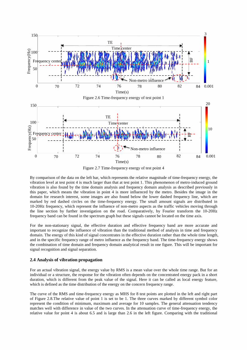
Figure 2.6 Time-frequency energy of test point 1

Figure 2.7 Time-frequency energy of test point 4

By comparison of the data on the left bar, which represents the relative magnitude of time-frequency energy, the

vibration level at test point 4 is much larger than that at test point 1. This phenomenon of metro-induced ground

vibration is also found by the time domain analysis and frequency domain analysis as described previously in

this paper, which means the vibration in point 4 is more influenced by the metro. Besides the image in the

domain for research interest, some images are also found below the lower dashed frequency line, which are

marked by red dashed circles on the time-frequency energy. The small amount signals are distributed in

10-20Hz frequency, which represent the influence of non-metro aspects as the traffic vehicles moving through

the line section by further investigation on the road. Comparatively, by Fourier transform the 10-20Hz

frequency band can be found in the spectrum graph but these signals cannot be located on the time axis.

For the non-stationary signal, the effective duration and effective frequency band are more accurate and

important to recognize the influence of vibration than the traditional method of analysis in time and frequency

domain. The energy of this kind of signal concentrates in the effective duration rather than the whole time length,

and in the specific frequency range of metro influence as the frequency band. The time-frequency energy shows

the combination of time domain and frequency domain analytical result in one figure. This will be important for

signal recognition and signal separation.

2.4 Analysis of vibration propagation

For an actual vibration signal, the energy value by RMS is a mean value over the whole time range. But for an

individual or a structure, the response for the vibration often depends on the concentrated energy pack in a short

duration, which is different from the peak value of the signal. Here it can be called as local energy feature,

which is defined as the time distribution of the energy on the concern frequency range.

The curve of the RMS and time-frequency energy as MHS for 8 test points are plotted in the left and right part

of Figure 2.8.The relative value of point 1 is set to be 1. The three curves marked by different symbol color

represent the condition of minimum, maximum and average for 10 samples. The general attenuation tendency

matches well with difference in value of the two curves. In the attenuation curve of time-frequency energy, the

relative value for point 4 is about 6.5 and is large than 2.6 in the left figure. Comparing with the traditional

3

0.001

1

Time(s)

Fre

qu

ency

(Hz)

Frequency center

20

0.001

10

Fre

qu

ency

(Hz)

Time center

BF

TE

Non-metro influence

70 72 74 82 76 78 80 84 0

100

50

150

Frequency center

Time center

BF

TE

Non-metro influence

70 72 74 82 76 78 80 84 0

100

50

150

Time(s)

index RMS, the time-frequency energy is more evident to show the local amplification phenomenon.

Figure 2.8 The relative value of RMS and MHS for vibration signals in 8 test points

3. CONCLUSION

This paper presents the analysis of time-frequency energy for metro induced environmental vibration by

Margenau-Hill-Spectrogram distribution. The signal can be characterized in the time-frequency plane by its

center position ( , )m mt f and a domain of time-frequency band product as TE BF . The evaluation index for

time-frequency energy is calculated and further discussed. Comparing with the traditional methods in the time

domain and the frequency domain, the time-frequency energy can directly show the characteristics of the signal

contents with convenience and reliability. By analysis of the time-frequency energy, the influence of the

non-metro aspects can be removed and the propagation law for environmental vibration induced by metro can

be got effectively. The environmental vibration is usually attenuated with the distance except local amplification

not far away. Using the time-frequency energy as the evaluation index rather than the RMS, the amplification

phenomenon in certain area is more evident with low variance of the data.

4. ACKNWLEDGMENT

Financial support from Shanghai National Science Foundation (No. 13ZR1444800) is gratefully acknowledged.

REFERENCES

1. Mao,Y.Q. (1987).Characteristics and Attenuation of Ground Vibration Caused by Traffic Vehicle. Journal

of Building Structures.8:1,54-60. (in Chinese)

2. Cui,G.H., Tao,X.X. and Chen,X.M.(2008).Actual Measurement and Analysis on Attenuation for

Environmental Vibration Induced by Urban Rail Transit on Ground. Journal of Shenyang Jianzhu

University(Natural Science) .24:1,39-43. (in Chinese)

3. Lak,M.A., Degrande, G. and Lombaert, G. (2011).The Effect of Road Unevenness on the Dynamic Vehicle

Response and Ground-borne Vibrations Due to Road Traffic. Soil Dynamic and Earthquake Engineering.

31:10,1357-1377.

4. Mhanna,M., Sadek,M. and Sharhrour,I.(2012).Numerical Modeling of Traffic-induced Ground Vibration.

Computers and Geotechnics.39:1,116-123.

5. Jia,B.Y.,Lou,M. L.,Zong,G. et al.(2013). Field Measurements for Ground Vibration Induced by Vehicle.

Journal of Vibration and Shock. 32:4,11-14. (in Chinese)

6. Ge,Z.X. and Chen,Z. S.(2006). Time-frequency Analysis Technology and Its Application by MATLAB

Software. Posts and Telecom Press. (in Chinese)

7. Zhang,B., Zong, G., Li, G.Z., et al.(2014).Time-Frequency Energy Evaluation Method of the Vibration

Induced by Underground Subway. Hans Journal of Civil Engineering.3:6,176-188.

8. Boualem, B. (2003).Time Frequency Signal Analysis and Processing. A Comprehensive Reference.

Prentice Hall.

9. Papandreou-Suppappola, A.(2003). Applications in Time-frequency Signal Processing. CRC Press.

10. Francois, A., Patrick, F., Paulo, G. and Olivier, L. (2005).Time-Frequency Toolbox for Use with MATLAB.

Tutorial and Reference Guide. (http://tftb.nongnu.org)

Distance(m) 60

1#

2

1#

80 60 20 40 20 40 80

8 Relative RMS Relative MHS

0

8#

6

4#

minimum

maximum

average

Distance(m)

6# 8#

4#

6#

4

0