Analysis of the Solvency II Standard Model …...AN ANALYSIS OF THE SOLVENCY II STANDARD MODEL...

Analysis of the Solvency II Standard ModelApproach to Longevity Risk

Matthias Borger

Preprint Series: 2009-21

Fakultat fur Mathematik und WirtschaftswissenschaftenUNIVERSITAT ULM

Deterministic Shock vs. Stochastic Value-at-Risk – An Analysis ofthe Solvency II Standard Model Approach to Longevity Risk!

Matthias BorgerInstitute of Insurance, Ulm University & Institute for Finance and Actuarial Sciences (ifa), Ulm

Helmholtzstraße 22, 89081 Ulm, Germany

Phone: +49 731 50 31230. Fax: +49 731 50 31239

Email: [email protected]

January 2010

PRELIMINARY VERSION

Abstract

In general, the capital requirement under Solvency II is determined as the 99.5% Value-at-Risk ofthe Available Capital. In the standard model’s longevity risk module, this Value-at-Risk is approximatedby the change in Net Asset Value due to a pre-specified longevity shock which assumes a 25% reductionof mortality rates for all ages.

We analyze the adequacy of this shock by comparing the resulting capital requirement to the Value-at-Risk based on a stochastic mortality model. This comparison reveals structural shortcomings of the25% shock and therefore, we propose a modified longevity shock for the Solvency II standard model.

We also discuss the properties of different Risk Margin approximations and find that they can yieldsignificantly different values. Moreover, we explain how the Risk Margin may relate to market pricesfor longevity risk and, based on this relation, we comment on the calibration of the cost of capital rateand make inferences on prices for longevity derivatives.

!The author is very grateful to Andreas Reuß, Jochen Ruß, Hans-Joachim Zwiesler, and Richard Plat for their valuable commentsand support, and to the Continuous Mortality Investigation for the provision of data.

1

AN ANALYSIS OF THE SOLVENCY II STANDARD MODEL APPROACH TO LONGEVITY RISK 2

1 Introduction

As part of the Solvency II project, the capital requirements for European insurance companies will be revisedin the near future.1 The main goal of the new solvency regime is a more realistic modeling and assessmentof all types of risk insurance companies are exposed to. In principle, the Solvency Capital Requirement(SCR) will then be determined as the 99.5% Value-at-Risk (VaR) of the Available Capital over a 1-year timehorizon, i.e., the capital required today to cover all losses which may occur over the next year with at least99.5% probability.Insurance companies are encouraged to implement (stochastic) internal models to assess their risks as accu-rately as possible. However, since the implementation of such internal models is rather costly and sophis-ticated, the European Commission with support of the Committee of Insurance and Occupational PensionSupervisors (CEIOPS) has established a scenario based standard model which all insurance companies willbe allowed to use in order to approximate their capital requirements. In this model, the overall risk is splitinto several modules, e.g. for market risk, operational risk, or life underwriting risk, and submodules forwhich separate SCRs are computed. These SCRs are then aggregated under the assumption of a multivariatenormal distribution with pre-specified correlation matrices to allow for diversification effects. The calibra-tion of the standard model is currently being established by a series of Quantitative Impact Studies (QIS) inwhich the effects of the new capital requirements are analyzed. Even though this standard model certainlyhas some shortcomings (for critical discussions see, e.g., Doff (2008) or Devineau and Loisel (2009)), mostsmall and medium-size insurance companies are expected to rely on this model. But also larger companiesare likely to adopt at least a few modules for their (partial) internal model. Hence, a reasonable implementa-tion and calibration of the standard model is crucial in order to ensure the financial stability of the Europeaninsurance markets.One prominent risk annuity providers and pension funds are particularly exposed to is longevity risk, i.e.the risk that insured on average survive longer than expected. The importance of this risk is very likelyto increase even further in the future: A general decrease in benefits from public pay as you go pensionschemes in most industrialized countries, often in combination with tax incentives for private annuitization,will almost certainly trigger a further increasing demand for annuity and endowment products. Moreover,longevity risk constitutes a systematic risk as it cannot be diversified away in a large insurance portfolio,and it is currently non-hedgeable since no liquid and deep market exists for the securitization of this risk.In the Solvency II standard model, longevity risk is explicitly accounted for as part of the life underwritingrisk module. The SCR is, in principle, computed as the change in liabilities due to a longevity shock thatassumes a permanent reduction of the mortality rates for all ages by 25%. The value of 25% is mainly basedon what insurance companies in the United Kingdom (UK) in 2004 regarded as consistent with the general99.5% VaR concept of Solvency II (cf. CEIOPS (2007)).However, the value as well as the structure of the longevity stress have come under some criticism lately.Some participants of QIS4 regard the longevity shock as very high (cf. CEIOPS (2008c)) and this is sup-ported by the fact that, in QIS4, internal models indicated, in median, a capital requirement for longevity

1For an overview and a discussion of the Solvency II proposals, we refer to Eling et al. (2007), Steffen (2008), and Doff (2008).A comparison with other solvency regimes can be found in Holzmuller (2009).


risk of only 81% of that based on the standard model (cf. CEIOPS (2008c)). One could argue that thisdifference in SCRs is desirable because the standard model approach is meant to be conservative in orderto give incentives for the implementation of internal models. Nevertheless, the longevity shock’s adequacyis questionable. A reason given by QIS4 participants for not applying the standard model is that “the formof the longevity stress within the SCR standard formula does not appropriately reflect the actual longevityrisk, specifically it does not appropriately allow for the risk of increases in future mortality improvements”(CEIOPS (2008c)). In its recent consultation paper, CEIOPS (2009a) acknowledges the feedback that agradual change in mortality rates may be more appropriate than a one-off shock and that the longevitystress should also depend on age and duration but nevertheless decides to stick to the 25% one-off shock.The consequence could be an unnecessarily high capitalization of insurance companies in case longevityrisk is overestimated by the 25% longevity shock, or in the converse case, a company’s default risk beingsignificantly higher than the accepted level of 0.5%.Therefore, a thorough analysis is required whether or not the change in liabilities due to a 25% longevityshock constitutes a reasonable approximation of the 99.5% VaR of the Available Capital. This analysis iscarried out in this paper. We examine the adequacy of the shock’s structure, i.e. an equal shock for all agesand maturities, and its calibration. Moreover, we explain how it could possibly be improved. In the secondpart of the paper, we discuss the Risk Margin under Solvency II for the case of longevity risk. Due to itscomplexity, different approximations have been proposed whose properties and performances are yet ratherunclear. We examine these approximations, in particular the assumption of a constant ratio of SCRs andliabilities over time which has turned out to be very popular in practice. Moreover, we contribute to theongoing debate on the calibration of the cost of capital rate by relating the Risk Margin to (hypothetical)market prices for longevity risk. This approach offers a new perspective compared to the shareholder returnmodels which have been applied in the calibration so far (cf. CEIOPS (2009b)). Using the same relationand assuming the cost of capital rate to be fixed, we can finally make inferences on the pricing of longevityderivates.The impact and the significance of longevity risk on annuity or pension portfolios have already been ana-lyzed by several authors. However, not all of their work directly relates to capital requirements under a par-ticular solvency regime. For instance, Plat (2009) focuses on the additional longevity risk pension funds canbe exposed to due to fund specific mortality compared to general population mortality. Stevens et al. (2008)compare the risks inherent in pension funds with different product mixes, and Dowd et al. (2006) measurethe remaining longevity risk in an annuity portfolio in case of imperfect hedges by various longevity bonds.Others, like Hari et al. (2008) and Olivieri and Pitacco (2008a,b), do analyze capital requirements for certainportfolios but consider approaches which differ from the 1-year 99.5% VaR concept of Solvency II, e.g. theyassume longer time horizons and different default probabilities. Therefore, no final conclusion regarding thestandard model approach is possible in their setting. Nevertheless, Olivieri and Pitacco (2008a,b) come tothe conclusion that the “shock scenario referred to by the standard formula can be far away from the actualexperience of the insurer, and thus may lead to a biased allocation of capital”. They find that the standardformula contains some strong simplifications and argue that internal models should be adopted instead. Atleast, the magnitude of mortality reductions should be recalibrated to capital requirements derived from an


exemplary internal model.The remainder of this paper is organized as follows: In Section 2, the relevant quantities, i.e. the AvailableCapital, the Risk Margin, and the Solvency Capital Requirement are defined. For the latter, different defini-tions based on the 25% longevity shock (the shock approach) and based on the VaR of the Available Capital(the VaR approach) are given. Moreover, the practical computation of these SCRs is described. Since thecomputation in the VaR approach requires stochastic modeling of mortality, in Section 3, we discuss the suit-ability of different mortality models and explain why we decided to use the forward model of Bauer et al.(2008, 2009a). Subsequently, we introduce the forward mortality modeling framework, in which this modelis specified. The full specification of the model and an improved calibration algorithm are presented in theappendix. In Section 4, we establish the setting in which the SCRs from both longevity stress approachesare to be compared. In particular, assumptions and simplifications are introduced which are necessary toexclude risks other than longevity risk and to ensure that a direct comparison of SCRs based on a one-offshock approach and a gradual change in mortality as in the model of Bauer et al. (2008, 2009a) is possi-ble. The comparison is then performed in Section 5. In the process, various term structures, ages, levels ofmortality rates, and portfolios of contracts are considered. Based on the observations, a modified longevitystress for the standard model is proposed in Section 6, which is still scenario based but allows for the shockmagnitude to depend on age and maturity. In Section 7, the Risk Margins based on the 25% shock andthe modified longevity stress are compared and the properties of different Risk Margin approximations areanalyzed. Moreover, we discuss the adequacy of the current cost of capital rate and argue how the pricing oflongevity derivatives may relate to the Solvency II capital requirements and the Risk Margin in particular.Finally, Section 8 concludes.

2 The Solvency Capital Requirement under Solvency II

2.1 General Definitions

Intuitively, the Solvency Capital Requirement (SCR) under Solvency II is defined as the amount of capitalnecessary at time t = 0 to cover all losses which may occur until t = 1 with a probability of at least99.5%. However, in order to give a precise definition of the SCR, we first need to introduce the notion ofthe Available Capital.By definition, the Available Capital at time t, ACt, is the difference between market value of assets andmarket value of liabilities at time t. Thus, it is a measure of the amount of capital which is available tocover future losses. In general, the market value of a company’s assets can be derived rather easily: Eitherasset prices are directly obtainable from the financial market (mark-to-market) or the assets can be valuedby well established standard methods (mark-to-model). However, the market value of liabilities is difficultto determine. There is no liquid market for such liabilities and due to options and guarantees embeddedin insurance contracts, the structure of the liabilities is typically rather complex such that standard modelsfor asset valuation cannot be applied directly. Therefore, under Solvency II a market value of liabilities isapproximated by the so-called Technical Provisions which consist of the Best Estimate Liabilities (BEL)and a Risk Margin (RM).


The Risk Margin can be interpreted as a loading for non-hedgeable risk and has to “ensure that the valueof technical provisions is equivalent to the amount that (re)insurance undertakings would be expected torequire to take over and meet the (re)insurance obligations” (CEIOPS (2008a)). Thus, in case of a company’sinsolvency the Risk Margin should be large enough for another company to guarantee the proper run-off ofthe portfolio of contracts. It is computed via a cost of capital approach (cf. CEIOPS (2008a)) and reflectsthe required return in excess of the risk-free return on assets backing future SCRs. Hence, the Risk MarginRM can be defined as (cf. CEIOPS (2009b))

RM :=!

t!0

CoC · SCRt

(1 + it+1)t+1 , (1)

where SCRt is the SCR at time t, it is the 1-year risk-free interest rate at time zero for maturity t, and CoC

is the cost of capital rate, i.e. the required return in excess of the risk-free return.The SCR is defined as the 99.5% VaR of the Available Capital over 1 year, i.e. the smallest amount x forwhich (cf. Bauer et al. (2009b))

P (AC1 > 0|AC0 = x) " 99.5%. (2)

However, since this implicit definition is rather unpractical in (numerical) computations, one often uses thefollowing approximately equal definition (cf. Bauer et al. (2009b))

SCRV aR := argminx

"P

#AC0 #

AC1

1 + i1> x

$$ 0.005

%. (3)

From Equations (1) and (3), a mutual dependence between Available Capital and SCR becomes obvious:The SCR is computed as the VaR of the Available Capital, and the Available Capital depends on the SCRvia the Risk Margin. In order to solve this circular relation, CEIOPS (2009a) states that – whenever a lifeunderwriting risk stress is based on the change in value of assets minus liabilities – the liabilities should notinclude a Risk Margin when computing the SCR. Thus, it is assumed that the Risk Margin does not changein stress scenarios and that the change in Available Capital can be approximated by the change in Net AssetValue

NAVt := At # BELt,

whereAt denotes the market value of assets andBELt the Best Estimate Liabilities at time t. For simplicity,we will refer to the latter as the liabilities only in what follows.

2.2 The Solvency Capital Requirement for Longevity Risk

As mentioned in the introduction, the Solvency II standard model follows a modular approach where themodules’ and submodules’ SCRs are computed separately and then aggregated according to pre-specifiedcorrelation matrices. Thus, for the submodule of longevity risk the SCR should, in principle, be computedas (cf. Equation (3))

SCRV aRlong := argminx

"P

#NAV0 #

NAV1

1 + i1> x

$$ 0.005

%, (4)


whereBELt andAt in the definition ofNAVt correspond to the liabilities of all contracts which are exposedto longevity risk and the associated assets, respectively.In the current specification of the Solvency II standard model, however, the SCR for longevity risk – as anapproximation of SCRV aR

long – is determined as the change in Net Asset Value due to a longevity shock attime t = 0 (cf. CEIOPS (2008a)), i.e.

SCRshocklong := NAV0 # (NAV0|longevity shock), (5)

The longevity shock is a permanent reduction of the mortality rates for each age by 25%. This shock is onlymeant to account for systematic changes in mortality and does not account for small sample risk.2 Therefore,we also disregard any small sample risk in the VaR approach as an inclusion would blur the results of ourcomparison in Section 5. In what follows, we only consider the SCR for longevity risk and thus omit theindex ·long for simplicity.

3 The Mortality Model

3.1 Model Requirements

The computation of the SCR for longevity risk via the VaR approach obviously requires stochastic modelingof mortality. In the literature, a considerable number of stochastic mortality models has been proposed andfor an overview we refer to Cairns et al. (2008). However, only very few of these models are suitable for thecomputation of a VaR over a 1-year time horizon.From an annuity provider’s perspective, longevity risk in the 1-year setting of Solvency II consists of twocomponents: First, there is the risk that next year’s realized mortality will be (significantly) below its ex-pectation, e.g., due to a mild winter with less people than usual dying from flu. The second component isthe risk of a decrease in expected mortality beyond next year, for which the cure of cancer is the classicalexample. A newly discovered medication against cancer would have to be tested thoroughly first and itwould take some time until it would be available to a group of people large enough such that mortality ona population scale would be affected. Thus, a noticeable effect on next year’s realized mortality is ratherunlikely. However, (long-term) mortality assumptions would certainly have to be revised. Both componentsof the longevity risk lead to higher than expected liabilities at t = 1 – in the first case, because more insuredwould still be alive than assumed and in the second case, because for those who are still alive liabilities att = 1 on a best estimate basis would be larger than anticipated at t = 0. Hence, in order to properly assesslongevity risk over a 1-year time horizon, a stochastic mortality model must account for both componentsof the risk.The most common mortality models belong to the class of spot models where only realized (period) mortal-ity is modeled. To account for anticipated changes in mortality over time (typically a decrease in mortalityis assumed), spot models contain a mortality trend assumption. However, in most spot models this trendis fixed as part of the calibration process and scenarios of realized mortality are derived as random devia-

2In the context of Solvency II, small sample risk is sometimes also referred to as mortality volatility risk.


tions from this trend. This means that the liabilities at t = 1 are always computed based on the same trendassumption and thus, these models do not account for the second component of the longevity risk.Cox et al. (2009) and Sweeting (2009) overcome the issue of a fixed trend by allowing for trend changesin the well-known mortality models of Lee and Carter (1992) and Cairns et al. (2006a), respectively. Theformer use a Markov regime switching model with different trend and volatility assumptions in the twomortality regimes under consideration. However, in their time-homogeneous Markov chain model, theanticipated long-term mortality trend depends to a diminishing extent on the current mortality regime andpossible regime switches in the next year but is rather fixed by the stationary distribution of the Markovchain. Hence, even though the model allows for more variability in simulated mortality paths, it doesnot sufficiently account for possible changes in the anticipated long-term mortality trend. In the modelof Sweeting (2009), each year, the trend parameters in the two stochastic factors can increase or decreaseby a fixed amount or remain constant. Thus, in contrast to the model of Cox et al. (2009), the currenttrend parameters always determine the best estimate mortality trend until infinity. However, due to onlythree possible scenarios for each trend parameter in a 1-year simulation, the range of possible overall trendchanges over one year is very limited. This makes a reasonable computation of a 99.5% quantile impossibleas, for such a computation to be sound, the distribution of the magnitude of trend changes would have tobe (at least approximately) continuous. Therefore, we conclude that also only very recently developed spotmodels which allow for trend changes are not directly applicable in the Solvency II framework.A class of mortality models which overcomes the outlined drawbacks of spot models are so-called forwardmortality models. Such models can be seen as an extension of spot models in the time/maturity dimension asthey require the expected future mortality as input and model changes in this quantity over time. Thus, theysimultaneously allow for random evolutions of realized mortality and for changes in the long-term mortalityexpectation. Even changes in expected mortality for only certain future time periods can be modeled incontrast to trend-varying spot models where changes in the trend parameters influence expected mortalityat all future points in time. This makes forward models usually more complex than spot models but for areasonable computation of a 1-year VaR this additional complexity seems inevitable. Moreover, even if onehad an adequate spot model at hand, a forward model would still offer the advantage that no nested simu-lations would be required for the computation of the liabilities at t = 1. In a forward modeling framework,these liabilities can be computed directly based on the current mortality surface, whereas, when using a spotmodel, for each 1-year simulation path another set of paths is needed to compute the liabilities by MonteCarlo simulation.For our analyses in the following sections, we use a slightly modified version of the forward mortality modelintroduced by Bauer et al. (2008, 2009a) which we refer to as the BBRZ model. Forward mortality modelshave been proposed by other authors as well (see, e.g., Dahl (2004), Miltersen and Persson (2005), or Cairnset al. (2006b)), however, as they do not provide concrete specifications of their models, to our knowledge,the BBRZ model is the only forward model which is readily available for practical applications. In thefollowing subsection, we introduce the forward mortality framework in which the BBRZmodel is specified.The full specification of the model is given in the appendix where also an improved calibration algorithm ispresented.


3.2 The Forward Mortality Framework

Following Bauer et al. (2008, 2009a), for the remainder of this paper we fix a time horizon T" and a filteredprobability space (!,F ,F, P ), where F = (F)0#t#T ! satisfies the usual conditions. Since we disregardany small sample risk in our setting, it is reasonable to assume a large but fixed underlying population ofindividuals, where each age cohort is denoted by the age x0 at time t0 = 0. We assume that the best estimateforward force of mortality with maturity T as from time t,

µt(T, x0) := # !

!Tlog

&EP

'T p(T )

x0

(((Ft

)*T>t= # !

!Tlog

&EP

'T$tp

(T )x0+t

(((Ft

)*, (6)

is well defined, where T$tp(T )x0+t denotes the proportion of (x0 +t)-year olds at time t $ T who are still alive

at time T , i.e. the survival rate or the “realized survival probability”. Moreover, we assume that (µt(T, x0))satisfies the stochastic differential equations

dµt(T, x0) = "(t, T, x0) dt + #(t, T, x0) dWt, µ0(T, x0) > 0, x0, T " 0, (7)

where (Wt)t!0 is a d-dimensional standard Brownian motion independent of the financial market, and"(t, T, x0) as well as #(t, T, x0) are continuous in t. Furthermore, the drift term "(t, T, x0) has to sat-isfy the drift condition (cf. Bauer et al. (2008))

"(t, T, x0) = #(t, T, x0) %+ T

t#(t, s, x0)% ds, (8)

which means that a forward mortality model is fully specified by the volatility #(t, T, x0) and the initialcurve µ0(T, x0).From definition (6), we can deduce the best estimate survival probability for an x0-year old to survive fromtime zero to time T as seen at time t:

EP

'T p(T )

x0

(((Ft

)= EP

'e$

, T0 µu(u,x0) du

(((Ft

)= e$

, T0 µt(u,x0) du. (9)

For t = 1, these are the survival probabilities we need to compute the liabilities and the Net Asset Valueafter one year. Note that µt(u, x0) = µu(u, x0) for u $ t since the volatility #(t, u, x0) must obviously beequal to zero for u $ t. Inserting the dynamics (7) into (9) yields

EP

'T p(T )

x0

(((Ft

)= EP

'T p(T )

x0

)% e$

, T0 (

, t0 !(s,u,x0) ds+

, t0 "(s,u,x0) dWs)du, (10)

which means that we actually do not have to specify the forward force of mortality. For our purposes, it issufficient to provide – besides the volatility #(s, u, x0) – best estimate T -year survival probabilities as attime t = 0 which can, from a technical point of view, be obtained from any generational mortality table.Given these quantities, we are able to compute the SCR for longevity risk via the VaR approach empiricallyby means of Monte Carlo simulation.Since we use a deterministic volatility (cf. appendix) the forward force of mortality is Gaussian. Hence, it


could become negative for extreme scenarios with survival probabilities becoming larger than 1. However,for the 50,000 paths we have randomly chosen for the empirical computation of the VaR in the subsequentanalysis such a scenario does not occur and therefore, we regard this as an negligible shortcoming forpractical considerations, even in tail scenarios.An appealing feature of the Gaussian setting is that – given a deterministic “market price of risk” process($(t))t!0 – the volatilities under the real world measure P and under the equivalent martingale measure Q

generated by ($(t))t!0 via its Radon-Nikodym density (see, e.g., Harrison and Kreps (1979) or Duffie andSkiadas (1994))

!Q

!P

((((Ft

= exp"+ t

0$(s)% dWs #

12

+ t

0&$(s)&2 ds

%,

coincide (cf. Bauer et al. (2008)). Hence, risk-adjusted survival probabilities, i.e. survival probabilities underthe measure Q, can easily be derived from their best estimate counterparts via

EQ

'T p(T )

x0

(((Ft

)

= EQ

'e$

, T0 µu(u,x0) du

(((Ft

)= EQ

'e$

, T0 (µt(u,x0)+

, ut !(s,u,x0) ds+

, ut "(s,u,x0) dWs)du

(((Ft

)

= e$, T0

, ut "(s,u,x0)#(s) ds du % EQ

'e$

, T0 (µt(u,x0)+

, ut !(s,u,x0) ds+

, ut "(s,u,x0) (dWs$#(s) ds))du

(((Ft

)

= e$, T0

, ut "(s,u,x0)#(s) ds du % EP

'T p(T )

x0

(((Ft

), (11)

since-Wt

.

t!0with Wt = Wt #

, t0 $(u) du is a Q-Brownian motion by Girsanov’s Theorem (see e.g.

Theorem 3.5.1 in Karatzas and Shreve (1991)). We will make use of this relation when we analyze the RiskMargin in Section 7.

4 The Model Setup

In this section, we describe the setting for our analysis of the longevity stress in the Solvency II standardmodel which includes assumptions on the interest rate evolution, the reference company’s asset strategy, thecontracts under consideration, as well as the best estimate mortality.Our reference company is situated in the UK and is closed to new business. We set t = 0 in 2007 andas risk-free interest rates we deploy the risk-free term structure for year-end 2007 provided by CEIOPS(2008b) as part of QIS4. For the approximative definition of the SCR (cf. Equation (3)) to coincide with theexact definition (cf. Equation (2)), we assume that the company’s assets and Technical Provisions coincideat t = 0. Thus, the company does not possess any Excess Capital. Since we want our company to be solelyexposed to longevity risk, we also assume that it only invests in risk-free assets and that it is completelyhedged against changes in interest rates. As a consequence of the latter, a deterministic approach for theinterest rate evolution is sufficient and the company specific risk-free term structure at time t can be deducedfrom the 2007 term structure. We denote by i(t, T ) the annual interest rate for maturity T at time t, t $ T .The risk-free assets are traded only when premium payments are received or survival benefits are paid andin each case the asset cash flow coincides with the liability cash flow. Hence, differing values of assets


and Technical Provisions at t > 0 are always and only due to changes in (expected) mortality. Finally, wedisregard any operational risk.As standard contracts we consider life annuities which pay a fixed annuity amount yearly in arrears if theinsured is still alive and which do not contain any options or guarantees for death benefits. Moreover, thereis no surplus participation and any charges are disregarded. Thus, in case an x0-year old at t0 = 0 is stillalive at time t, the liabilities of such a contract paying £1 are

BELt =!

T>t

1(1 + i(t, T ))T$t

· EP

'T p(T )

x0

(((Ft

).

The best estimate survival probabilities at t = 0 are derived from the basis table PNMA00 for UK LifeOffice Pensioners,3 and a projection according to the average of projections used by 5 large UK insurancecompanies in 2006. For details on this average projection, we refer to Bauer et al. (2009a) and Grimshaw(2007).As a consequence of the assumptions on payment dates and the asset evolution, we have

A1 = A0 (1 + i(0, 1)) + CF1, (12)

where CF1 denotes the company’s (stochastic) cash flow at t = 1. This cash flow is negative in case thecompany pays more benefits than it receives premiums and positive otherwise. Equation (12) implies that

NAV0 #NAV1

1 + i(0, 1)=

BEL1 # CF1

1 + i(0, 1)# BEL0,

and hence, the SCR formula in the VaR approach, Equation (4), simplifies to

SCRV aR = argminx

"P

#BEL1 # CF1

1 + i(0, 1)# BEL0 > x

$$ 0.005

%. (13)

Thus, we can disregard the evolution of the assets in our computations. Also the SCR formula in the shockapproach, Equation (5), can be reformulated in terms of the liabilities:

SCRshock = (BEL0|longevity shock) # BEL0. (14)

From these simplified SCR formulas, an important observation can be made: Since, in our setting, cashflows occur only yearly, the SCR in the VaR approach only depends on the expected mortality at the end ofthe first year, i.e. at t = 1. Hence, it does not matter whether changes in mortality emerge gradually overthe year or in a one-off shock at t = 0. Moreover, every gradual mortality evolution can be expressed in aone-off shock at t = 0, namely in a shock which transforms the expected survival probabilities at t = 0 intothe ones obtained at t = 1 via the gradual evolution. Therefore, if we express a longevity scenario which

3The table PNMA00 is part of the ’00’ series of mortality tables and contains amounts based mortality rates for normal entriesin 2000.


BEL0 BEL1 # CF1 SCR SCR/BEL0

Shock approach 12619.28 14238.81 869.87 6.9%VaR approach 12619.28 14050.62 691.59 5.5%

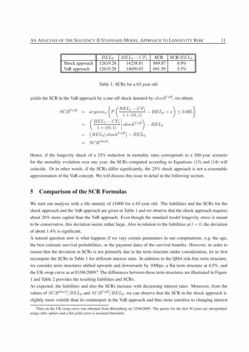
Table 1: SCRs for a 65-year old

yields the SCR in the VaR approach by a one-off shock denoted by shockV aR, we obtain

SCRV aR = argminx

"P

#BEL1 # CF1

1 + i(0, 1)# BEL0 > x

$$ 0.005

%

=#

BEL1 # CF1

1 + i(0, 1)

(((( shockV aR

$# BEL0

=/BEL0| shockV aR

0# BEL0

= SCRshock.

Hence, if the longevity shock of a 25% reduction in mortality rates corresponds to a 200-year scenariofor the mortality evolution over one year, the SCRs computed according to Equations (13) and (14) willcoincide. Or in other words, if the SCRs differ significantly, the 25% shock approach is not a reasonableapproximation of the VaR concept. We will discuss this issue in detail in the following section.

5 Comparison of the SCR Formulas

We start our analysis with a life annuity of £1000 for a 65-year old. The liabilities and the SCRs for theshock approach and the VaR approach are given in Table 1 and we observe that the shock approach requiresabout 26% more capital than the VaR approach. Even though the standard model longevity stress is meantto be conservative, this deviation seems rather large. Also in relation to the liabilities at t = 0, the deviationof about 1.4% is significant.A natural question now is what happens if we vary certain parameters in our computations, e.g. the age,the best estimate survival probabilities, or the payment dates of the survival benefits. However, in order toensure that the deviation in SCRs is not primarily due to the term structure under consideration, let us firstrecompute the SCRs in Table 1 for different interest rates. In addition to the QIS4 risk-free term structure,we consider term structures shifted upwards and downwards by 100bps, a flat term structure at 4.5%, andthe UK swap curve as at 01/06/2009.4 The differences between these term structures are illustrated in Figure1 and Table 2 provides the resulting liabilities and SCRs.As expected, the liabilities and also the SCRs increase with decreasing interest rates. Moreover, from thevalues of SCRshock/BEL0 and SCRV aR/BEL0, we can observe that the SCR in the shock approach isslightly more volatile than its counterpart in the VaR approach and thus more sensitive to changing interest

4Data on the UK swap curve was obtained from Bloomberg on 12/06/2009. The quotes for the first 30 years are interpolatedusing cubic splines and a flat yield curve is assumed thereafter.


2%

3%

4%

5%

6%

10 20 30 40 50

i(0,

T)

T

QIS4 term structureQIS4 term structure – 100bpsQIS4 term structure + 100bps

Flat term structure (4.5%)UK swap curve 01/06/2009

Figure 1: Different term structures for SCR computation

Term structure BEL0 SCRshock SCRshock

BEL0SCRV aR SCRV aR

BEL0

!SCRSCRV aR

QIS4 12619.28 869.87 6.9% 691.59 5.5% 25.8%QIS4 - 100bps 14002.91 1090.17 7.8% 848.91 6.1% 28.4%QIS4 + 100bps 11448.34 701.71 6.1% 569.47 5.0% 23.2%Flat (4.5%) 13040.42 887.65 6.8% 710.19 5.5% 25.0%Swap 01/06/2009 13646.54 950.05 7.0% 753.73 5.5% 26.0%

Table 2: SCRs for different term structures

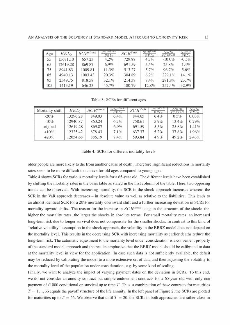
rates. Nevertheless, the relative deviation between the SCRs5 remains rather constant as can be seen in thelast column and hence, the interest rates obviously do not have a significant impact on our analysis.In order to analyze the SCRs for different ages, we consider ages between 55 and 105 as given in the firstcolumn of Table 3. In the third and fourth column we see that the SCR in the shock approach first increaseswith age and then decreases again and that the SCR relative to the liabilities BEL0 becomes rather large forvery old ages. These observations are due to the structure of the longevity shock since the effect of the 25%reduction increases as the mortality rates increase. In the VaR approach, the SCR decreases with age anddecreasing liabilities, and only the ratio of SCR and liabilities increases which seems more intuitive. In thelast two columns, we can observe that for ages above 85, the SCR in the shock approach more than triplesthe SCR in the VaR approach and also in relation to the liabilities the deviation is huge. These observationsclearly question the adequacy of the longevity stress in the standard model.On the other hand, for age 55 the SCR for the current shock calibration is already smaller than its counterpartin the VaR approach. Therefore, a simple adjustment of the shock’s magnitude such that the SCRs for oldages approximately coincide may lead to a significant underestimation of the longevity risk for youngerages. Hence, the shortcoming of the standard model longevity stress seems to be more a structural one and,in principle, an age-dependent stress with smaller relative reductions for old ages might be more appropriate.This coincides with epidemiological findings: The number of relevant causes of death is larger for old agesthan for young ages (cf. Tabeau et al. (2001)) which means that even if some cause of death is contained,

5For the remainder of this text, we define the relative deviation as !SCRSCRV aR = SCRshock"SCRV aR

SCRV aR .


Age BEL0 SCRshock SCRshock

BEL0SCRV aR SCRV aR

BEL0

!SCRSCRV aR

!SCRBEL0

55 15671.10 657.23 4.2% 729.88 4.7% -10.0% -0.5%65 12619.28 869.87 6.9% 691.59 5.5% 25.8% 1.4%75 8941.83 1009.81 11.3% 513.27 5.7% 96.7% 5.6%85 4940.13 1003.43 20.3% 304.89 6.2% 229.1% 14.1%95 2549.75 818.58 32.1% 214.38 8.4% 281.8% 23.7%105 1413.19 646.23 45.7% 180.79 12.8% 257.4% 32.9%

Table 3: SCRs for different ages

Mortality shift BEL0 SCRshock SCRshock

BEL0SCRV aR SCRV aR

BEL0

!SCRSCRV aR

!SCRBEL0

-20% 13296.28 849.03 6.4% 844.65 6.4% 0.5% 0.03%-10% 12940.87 860.24 6.7% 758.61 5.9% 13.4% 0.79%original 12619.28 869.87 6.9% 691.59 5.5% 25.8% 1.41%+10% 12325.42 878.43 7.1% 637.37 5.2% 37.8% 1.96%+20% 12054.68 886.19 7.4% 593.84 4.9% 49.2% 2.43%

Table 4: SCRs for different mortality levels

older people are more likely to die from another cause of death. Therefore, significant reductions in mortalityrates seem to be more difficult to achieve for old ages compared to young ages.Table 4 shows SCRs for various mortality levels for a 65-year old. The different levels have been establishedby shifting the mortality rates in the basis table as stated in the first column of the table. Here, two opposingtrends can be observed. With increasing mortality, the SCR in the shock approach increases whereas theSCR in the VaR approach decreases – in absolute value as well as relative to the liabilities. This leads toan almost identical SCR for a 20% mortality downward shift and a further increasing deviation in SCRs formortality upward shifts. The reason for the increase in SCRshock is again the structure of the shock: thehigher the mortality rates, the larger the shocks in absolute terms. For small mortality rates, an increasedlong-term risk due to longer survival does not compensate for the smaller shocks. In contrast to this kind of“relative volatility” assumption in the shock approach, the volatility in the BBRZ model does not depend onthe mortality level. This results in the decreasing SCR with increasing mortality as earlier deaths reduce thelong-term risk. The automatic adjustment to the mortality level under consideration is a convenient propertyof the standard model approach and the results emphasize that the BBRZ model should be calibrated to dataat the mortality level in view for the application. In case such data is not sufficiently available, the deficitmay be reduced by calibrating the model to a more extensive set of data and then adjusting the volatility tothe mortality level of the population under consideration, e.g. by some kind of scaling.Finally, we want to analyze the impact of varying payment dates on the deviation in SCRs. To this end,we do not consider an annuity contract but simple endowment contracts for a 65-year old with only onepayment of £1000 conditional on survival up to time T . Thus, a combination of these contracts for maturitiesT = 1, .., 55 equals the payoff structure of the life annuity. In the left panel of Figure 2, the SCRs are plottedfor maturities up to T = 55. We observe that until T = 20, the SCRs in both approaches are rather close in


0

5

10

15

20

25

30

35

10 20 30 40 50

SCR

T

Absolute SCRs

Shock approachVaR approach

-10%0%10%20%30%40%50%60%70%80%90%

10 20 30 40 50

Relativedeviation

T

Relative deviation in SCRs

Figure 2: SCRs for 1-year endowment contracts with maturity T

050100150200250

50 60 70 80 90 100

Amountinsured

x0

Figure 3: Age composition of the portfolio of immediate annuity contracts

absolute value. Thereafter, the shock approach demands significantly more SCR which explains the largerSCR for the life annuity. Finally, the SCRs in both approaches converge to zero due to an extremely lowprobability of survival. Note though that in the VaR approach the sum of SCRs in Figure 2 is about 5%larger than the SCR for the corresponding life annuity because diversification between different maturitiesis disregarded when computing the SCR for each endowment separately. Since the stress in the standardmodel does not allow for any diversification, in the shock approach, the sum of the SCRs for the endowmentscoincides with the SCR for the life annuity. In the right panel of Figure 2, the relative deviation in SCRsis displayed. It varies considerably over time ranging from about -10% to more than 80%. Hence, we canconclude that a longevity stress independent of the maturity under consideration is not adequate.Having considered single contracts only so far, we now want to investigate if the depicted shortcomings ofthe standard model longevity stress also lead to deviating SCRs for a realistic portfolio of immediate lifeannuities.6 In order to ensure a reasonable age composition, we choose a portfolio according to ContinuousMortality Investigation (CMI) data on the amounts based exposures of UK Life Office Pensioners in 2006.We only consider males and normal entries and rescale the data by dividing by 100,000 to obtain results ina handy range. The age composition of the portfolio is illustrated in Figure 3.From Table 5, we observe that the SCR in the shock approach more than doubles the SCR in the VaRapproach. Given the age composition of the portfolio, this is consistent with the observed SCRs for differentages (see Table 3). Thus, the aforecited structural shortcomings of the standard model longevity stress also

6Note that the presented results also hold true for a portfolio of deferred annuities in their payout phases.




Table 5: SCRs for a portfolio of immediate life annuities

Age BEL0 SCRshock SCRshock

BEL0SCRV aR SCRV aR

BEL0

!SCRSCRV aR

!SCRBEL0

30 3205.97 217.90 6.8% 382.66 11.9% -43.1% -5.1%35 3851.54 268.30 7.0% 428.53 11.1% -37.4% -4.2%40 4623.92 329.89 7.1% 489.79 10.6% -32.7% -3.5%45 5549.28 404.85 7.3% 561.71 10.1% -27.9% -2.8%50 6676.64 495.51 7.4% 631.44 9.5% -21.5% -2.0%55 8100.16 604.29 7.5% 688.98 8.5% -12.3% -1.1%60 9978.02 733.27 7.4% 724.06 7.3% 1.3% 0.1%

Table 6: SCRs for deferred annuities at different ages

affect the SCR for a realistic portfolio of contracts. According to Table 5, an insurance company whichapplies the standard model would have to raise additional solvency capital of about 6% of its liabilitiescompared to a company which implements the BBRZ model for VaR computation in an internal model.This is a huge amount given that, according to a stylized balance sheet for all undertakings in QIS4, NetAsset Value accounts for only about 18% of the total liabilities (cf. CEIOPS (2008c)).When analyzing the SCRs for different ages, we found that the relation between the SCRs seems to turnaround for young ages. To further investigate this, we consider deferred life annuities for different ageswhich again pay £1000 in arrears starting at age 65. Table 6 contains the corresponding SCRs.The SCRs increase in absolute value with age and for age 60, the SCRs in both approaches almost coincide.However, for younger ages the SCR in the VaR approach is (significantly) larger than the one in the shockapproach with the relative deviation growing, the younger the age under consideration. Here, the longevitystress in the standard model seems to (significantly) underestimate the longevity risk. Thus, we again findthat a longevity shock independent of age does not seem appropriate.As for the immediate annuities, we also want to analyze the consequences of the highlighted shortcomingsof the shock approach for a realistic portfolio of deferred annuity contracts. We derive the age compositionof our portfolio from CMI data on lives based exposures of male UK Personal Pensioners in 2006 and weonly consider data for pension annuities in deferment and for ages starting from 20 as the BBRZmodel doesnot cover ages below 20.7 Moreover, we assume yearly benefits in arrears of £0.01 for all contracts to keepall values in a handy range. The resulting overall amount insured for each age is displayed in Figure 4. Thebenefit payments are assumed to commence at age 65 or, in case age 65 has already been reached, after onemore year of deferment.

7Obviously, amounts based exposures would have been preferable because then no assumption on the benefit amount would benecessary, but such data is not available. The omission of ages below 20 is unproblematic for our purposes as exposures for thoseages are very small in the CMI data.


0100200300400500600

20 30 40 50 60 70 80

Amountinsured

x0

Figure 4: Age composition of the portfolio of deferred annuity contracts



Table 7: SCRs for a portfolio of deferred life annuities

The results in Table 7 confirm the observation for single ages that the shock approach demands significantlyless SCR for young ages.8 The significance of this difference is underlined by the fact that the shock SCR of6629.31 corresponds to a 1.5% default probability in the VaR approach. Thus, under the assumption that theBBRZ model assesses longevity risk correctly, the true default probability of our reference company wouldbe three times as large as accepted, if the company used the Solvency II standard model.For a combined portfolio of immediate and deferred annuities the deviations in SCRs from the two ap-proaches for different ages and maturities would obviously cancel each other out to some extent. Thus,despite its depicted structural shortcomings the standard model longevity stress may yield a reasonableoverall value for the longevity SCR in some cases. However, there are insurance companies in the marketwhose portfolios have a strong focus on certain age groups and therefore, an equal reduction of mortalityrates for all ages and maturities does not seem appropriate for the Solvency II standard model. To furtherillustrate this, we can cite the magnitudes of shocks which would yield SCRs for the two considered portfo-lios equal to those in the VaR approach. For the immediate annuities, a shock of about 13.0% would havebeen sufficient, whereas for the deferred annuities, a shock of about 29.4% would have been required.Therefore, in the following section we propose a modification of the longevity stress in the standard model,which overcomes the shortcomings of the current approach but does still not require stochastic simulationof mortality.

8A further analysis showed that premium payments during the deferment period do not have a significant effect on the SCRs. Tothis end, we assumed a start of premium payments at age 40 but at least three years ago (for ages below 43), and fixed the premiumamount such that an annuity certain could be paid for 15 years (as a proxy for the life annuity). Moreover, we included a margin of10% in the premium calculation. Obviously, in this setting, the liabilities were much lower, but the SCRs changed only slightly.


6 A Modification of the Standard Model Longevity Stress

In this section, we explain how the longevity stress in the Solvency II standard model could be modified inorder to overcome the shortcomings highlighted in the previous section which result from an equal shockfor all ages and maturities.We keep the structure of a one-off shock which means the integration of the longevity stress into the standardmodel does not change. From our point of view, such a one-off shock is an acceptable approximation ofgradual changes in expected mortality over only one year as the distinction between a one-off and a gradualmortality evolution only affects cash flows (premium payments and/or survival benefits) during the firstyear. Cash flows thereafter only depend on the expected mortality at t = 1 and not on how this expectationemerged (cf. Section 4). Regarding the cash flows in the first year, we see in the left panel of Figure 2that the corresponding SCR is typically very small compared to those for later years. Furthermore, theimplementation of gradual mortality changes would make the standard model more complex as, currently,all risks other than longevity risk are implicitly excluded by computing the shocked liabilities at t = 0.We modify the longevity shock according to the volatility in the BBRZ model which introduces a depen-dency structure of the shock magnitude on age and maturity. Instead of the 1-year mortality rates, we nowshock the T -year survival probabilities by setting each probability to its individual 99.5% quantile in a 1-yearsimulation of the BBRZmodel. From Equation (10), factors can easily be derived for each age and maturitywhich, when multiplied with the best estimate T -year survival probabilities, yield the desired percentiles.Thus, once the BBRZ model is calibrated, supervisory authorities would only have to provide insurancecompanies with a matrix of these factors and the computational efforts for calculating the SCR based on thismodified shock would basically remain as in the 25% shock approach.In principle, the modified shock yields an SCR which is larger than the one in the VaR approach sinceany diversification effects between different ages and maturities are disregarded when computing the 99.5%quantiles of each survival probability individually. In case of the portfolios considered in the previoussection, this gives a markup of about 5.2% of the SCR for the immediate annuities and of about 9.4%for the deferred annuities. However, given the considerable structural improvement of the modified shockcompared to the original 25% shock, we regard this inaccuracy as acceptable. Moreover, since the longevitystress in the standard model is supposed to be conservative in order to give incentives for the implementationof internal models, such a markup might actually be desirable. From this perspective, the modified shockoffers the additional advantage that a markup is distributed over all ages and maturities according to theactual risk, whereas, in the 25% shock, this distribution is not directly risk-related.As indicated in the previous section, the BBRZ model implies the application of an absolute volatilityand obviously, the same holds for the modified shock. The shock factors are only adequate as long asthe mortality level in the insurance portfolio in view (approximately) coincides with the level of mortalityexperience to which the BBRZ model has been calibrated. However, this drawback could be dealt with bycalibrating the BBRZ model to the mortality experience of different populations (with different mortalitylevels) such that the resulting shock factors allow for possibly different risk profiles – in magnitude as wellas in structure.In case the provision of a matrix of shock factors is regarded unpractical or too complex for the standard


0 20 40 60 80 100

T

20406080

100120

x0

-7

-5

-3

-1

1

-9-7-5-3-11

Figure 5: Log log of factors for modified shock approach

model, the surface formed by the factors could be approximated by a function of age and maturity. Thenonly this function would have to be provided by the supervisory authorities. Figure 5 shows the log log ofthe shock factors in the current calibration of the BBRZ model for all feasible combinations of initial agesx0 and maturities T . At first sight, the surface looks like a fairly even plane for all maturities T " 10.Therefore, a function of the form exp {exp {f(x0, T )}} might be applicable as an approximation of theshock factors, where f(x0, T ) is a plane with a correction for short maturities.9 However, the surface ofthe shock factors may look different for a different calibration of the BBRZ model and hence, also thisapproximating function might have to be derived individually for each population in view. We leave thisquestion for future work.Figure 6 shows the ratio of shock factors for T -year survival probabilities based on the modified shockand the original 25% shock of the mortality rates. Since the magnitude of the original shock depends onthe level of the mortality rates a general comparison is not possible. Here, we apply the 25% reduction tothe aforementioned Life Office Pensioners mortality table. We observe that for combinations of ages up toabout 60 and maturities up to about 50 the shocks are very similar. However, for higher initial ages the ratiosdecrease significantly which means the modified shock demands significantly less SCR for those ages. Onthe other hand, for rather young initial ages and long maturities, the ratios increase rapidly, which meansthe 25% shock may significantly underestimate the risk of changes in long-term mortality trends.10 Theseobservations are in line with those made in Section 5.

9The fitting of such a function would also allow for an extrapolation of the shock factors to ages below 20 for which the volatilityin the BBRZ model as specified in Bauer et al. (2008) is not defined.

10Note that the ratios are only displayed for maturities T up to 70 in Figure 6. For larger maturities the ratios increase further asone may anticipate. We do not plot them here because then, observations for shorter maturities would be difficult to make due tothe resulting scaling of the graph.


0 10 20 30 40 50 60 70T 2040

6080

100120

x0

0.5

1

1.5

2

0.20.40.60.811.21.41.61.82

Figure 6: Ratio of shock factors from modified and 25% longevity shock

7 The Risk Margin for Longevity Risk

7.1 Risk Margin Approximations

In Section 5, we found structural shortcomings of the longevity stress currently implemented in the SolvencyII standard model. These shortcomings may also affect the Risk Margin which is computed as the cost ofcapital for future SCRs in the run-off of an insurance portfolio (cf. Equation (1)). We will now analyze thispoint by comparing the Risk Margin in the 25% shock approach with its counterpart in the modified shockapproach (as a proxy of the VaR approach) introduced in the previous section.However, an exact computation of the Risk Margin would require the determination of each year’s SCR,SCRt, conditional on the mortality evolution up to time t. Since this is practically impossible, the RiskMargin is usually approximated. In the literature and in CEIOPS (2008a) in particular, several such approx-imations have been proposed and we will consider the following four:

(I) Approximation of the SCRt by assuming a mortality evolution up to time t according to its bestestimate. Thus, we have

RM (I) =!

t!0

CoC

(1 + i(0, t + 1))t+1· SCRBE

t .

In practice, this calculation method is generally seen as yielding the “exact” Risk Margin and there-fore, we are going to use it as a benchmark for the other approximation methods.

(II) Approximation of the SCRt using the proxy formula in CEIOPS (2008a, TS.XI.C.9), i.e.

RM (II) =!

t!0

CoC

(1 + i(0, t + 1))t+1· 25% · qav

t · 1.1(durt$1)/2 · durt · BELt,

where qavt is the expected average 1-year death rate at time t weighted by sum assured and durt is the


25% longevity shock Modified longevity shockPortfolio Method BEL0 RM Rel. dev. RM

BEL0RM Rel. dev. RM

BEL0

(I) 36394.73 2383.87 6.6% 1143.08 3.1%Immediate (II) 36394.73 2751.71 15.4% 7.6% n/a n/a n/aannuities (III) 36394.73 1957.24 -17.9% 5.4% 988.11 -13.6% 2.7%

(IV) 36394.73 2051.70 -13.9% 5.6% 1035.80 -9.4% 2.9%(I) 88165.37 11240.74 12.8% 12159.44 13.8%

Deferred (II) 88165.37 10126.91 -9.9% 11.5% n/a n/a n/aannuities (III) 88165.37 10034.70 -10.7% 11.4% 13206.71 8.6% 15.0%

(IV) 88165.37 10488.60 -6.7% 11.9% 13804.08 13.5% 15.7%

Table 8: Risk Margins for different portfolios, approximation methods, and longevity shocks

modified duration of the liabilities at time t.

(III) Approximation of the SCRt as the fraction SCR0/BEL0 of the liabilities BELt, i.e. assuming aconstant ratio of SCRs and liabilities over time (cf. CEIOPS (2008a, TS.II.C.28)):

RM (III) =!

t!0

CoC

(1 + i(0, t + 1))t+1· SCR0

BEL0· BELt.

(IV) Direct approximation of the Risk Margin via the modified duration of the liabilities (cf. CEIOPS(2008a, TS.II.C.26)):

RM (IV ) = CoC · dur0 · SCR0.

Table 8 contains the Risk Margins for the 25% longevity shock and the modified longevity shock, the twoportfolios of annuity contracts and all four approximation methods as far as they are well defined. Thecost of capital rate CoC is set to its current calibration in the Solvency II standard model, i.e. 6%. For themodified longevity shock, approximation method (II) is obviously not applicable since it is based on the25% shock of the mortality rates. Also note that this method is actually not admissible for the portfolio ofdeferred annuities because the average age in this portfolio does not reach the required 60 years (cf. CEIOPS(2008a)). Thus, the value for the deferred annuities in case of a 25% shock is only given for comparison.Regarding the two portfolios, we find that the Risk Margin in relation to the liabilities is generally largerfor the portfolio of deferred annuities which seems reasonable given the more long-term risk resulting inlarger uncertainty. This finding is supported by the graphs in the left panels of Figure 7 where the evolutionsof the best estimate SCRs (as in approximation method (I)) are displayed for both portfolios and shockapproaches.11 For the immediate annuities, the SCRs decrease toward zero quite directly whereas for thedeferred annuities, the SCRs first increase before fading out as less and less insured survive.Furthermore, for the “exact” calculation method (I), we observe that, in the case of the immediate annuities

11In order to determine effects which are only due to the inverse QIS4 term structure, we performed the calculations for Figure7 with different term structures. However, the resulting graphs differed only very slightly and thus, the effects of the term structureunder consideration can be regarded as insignificant.


050010001500200025003000350040004500

0 10 20 30 40 50 60 70 80

SC

Rt

t

Absolute SCRs – Immediate annuities portfolio

25% shockModified shock

0%

5%

10%

15%

20%

25%

30%

35%

0 10 20 30 40 50 60 70 80

SC

Rt/

BE

Lt

t

Relative SCRs – Immediate annuities portfolio


0

2000

4000

6000

8000

10000

12000

0 10 20 30 40 50 60 70 80 90 100

SC

Rt

t

Absolute SCRs – Deferred annuities portfolio


0%

5%

10%

15%

20%

25%

30%

35%

0 10 20 30 40 50 60 70 80 90 100

SC

Rt/

BE

Lt

t

Relative SCRs – Deferred annuities portfolio


Figure 7: Evolution of the SCRs in portfolio run-offs

portfolio, the Risk Margin in the 25% shock approach more than doubles its counterpart in the modifiedshock approach. This is not surprising as we have observed the same relation for the SCRs at t = 0 (seeTable 5). Moreover, in the top left panel of Figure 7, we can see that this relation holds thereafter as well.For the portfolio of deferred annuities, however, the Risk Margins are similar even though the SCRs at t = 0differ significantly (see Table 7). Here, a compensation over time occurs which becomes obvious in thebottom left panel of Figure 7: The higher SCRs in the modified shock approach for smaller t to some extentcompensate for the smaller SCRs later on, i.e. when the portfolio becomes similar to the immediate annuitiesportfolio. Nevertheless, depending on the portfolio under consideration, the structural shortcomings of the25% shock also adversly affect the Risk Margin.With respect to the Risk Margin approximations we find that they seem rather crude in general with theclosest approximation still being about 6.7% away from the “exact” value. However, compared to the largeuncertainty regarding the correct cost of capital rate (cf. CEIOPS (2009b)) and the value from calculationmethod (I) itself only being an approximation of unknown accuracy, the deviations appear less significant.Nevertheless, we think that the wide range of values for the approximated Risk Margin for each portfolioand longevity shock combination is problematic. The Solvency II regime is supposed to ease and improvecomparisons of the solvency situations of European insurance companies, but such comparisons might getblurred simply by the use of different Risk Margin approximations. Moreover, instead of assessing their riskas accurately as possible, insurance companies might be tempted to apply the Risk Margin approximationwhich yields the smallest value.Finally, we have a closer look at the Risk Margin for approximation method (III) which is very popular in


Portfolio 25% longevity shock Modified longevity shockof contracts RM $ RM $

Immediate annuities 2383.87 18.6% 1143.08 13.2%Deferred annuities 11240.74 8.7% 12159.44 8.9%

Table 9: Risk Margins and corresponding Sharpe ratios $

practice. From Table 8, we observe that the assumption, that future SCRs are proportional to future liabil-ities, results in the largest deviations in three of the four combinations of portfolios and longevity shocks.In each of these cases, the “exact” Risk Margin is underestimated. This is due to the ratio SCR0/BEL0

being a very crude if not inadequate proxy for ratios of future SCRs and liabilities as can be seen in theright panels of Figure 7. For both portfolios and both longevity shocks, the ratio is not even approximatelyconstant but, in general, increases with time.12 Thus, approximation method (III) does not seem appropriatein its current form. However, an adjustment of the proxy, e.g., in form of a dependence on the average agein the portfolio may improve results considerably.

7.2 The Cost of Capital Rate

As already indicated, there is a large uncertainty and hence, an ongoing discussion regarding the correct costof capital rate. It is currently set to 6%, but in CEIOPS (2009b) and references therein, values between 2%and 8% have been derived from different shareholder return models. An alternative idea for the calibrationof the cost of capital rate has been brought forward by Olivieri and Pitacco (2008c) who rely on reinsurancepremiums. However, since data on such premiums is not sufficiently available their idea is currently moreof theoretical interest.In what follows, we take a different approach to finding an adequate cost of capital rate. We compare theRisk Margin based on the current rate to hypothetical market prices of longevity dependent liabilities. Sincethe Risk Margin is supposed to provide a risk adjustment of the Best Estimate Liabilities it should coincidewith the markup of the risk-adjusted liabilities over their best estimate counterparts in such a market. Thisidea is also in line with the Risk Margin’s more specific interpretation in the cost of capital setting, i.e. theprovision of sufficient capital to guarantee an proper run-off of a portfolio. If a market for longevity riskexisted an insolvent insurer could guarantee the portfolio run-off by transferring the risk to the market at thecost of the Best Estimate Liabilities and the Risk Margin.We assume that, in the hypothetical longevity market, risk-adjusted survival probabilities are derived fromtheir best estimate counterparts as explained in Section 3. For the market price of longevity risk process$(t), we assume a time-constant Sharpe ratio $, i.e. the simplest possible process, since currently, thereis no information available on the structure of a market price of longevity risk process (cf. Bauer et al.(2009a)). The comparison is then performed by finding the Sharpe ratio which yields a markup in theliabilities coinciding with the cost of capital Risk Margin.Table 9 shows the Risk Margins and the corresponding Sharpe ratios for all combinations of portfolios and

12This observation is in line with the findings of Haslip (2008) for non-life insurance.


longevity shocks. For each portfolio, we observe that the Sharpe ratios increase with the Risk Margin whichis what one would expect. Moreover, we see that the Sharpe ratios for the deferred annuities are smallerthan those for the immediate annuities. Since the Sharpe ratios are chosen such that the markups in thehypothetical longevity market coincide with the Risk Margins, this means that the risk adjustment of thesurvival probabilities perceives a larger risk in the longer maturities of the deferred annuities than the RiskMargin does. Nevertheless, we observe that the Sharpe ratios are all of reasonable magnitude. For themodified longevity shock, where the computation of the Risk Margin and the risk-adjustment of the survivalprobabilities are performed based on (essentially) the same model/volatility, the Sharpe ratios do not seemtoo large in particular. For comparison, Bauer et al. (2009a) find that Sharpe ratios for longevity risk mightlie somewhere between 5% and 17% and Loeys et al. (2007) regard a value of 25% as reasonable. Themoderate values of $ we have found suggest that, at least in the case of longevity risk, the current cost ofcapital rate of 6% is not overly conservative. This is particularly the case if we take into account that, ina shock scenario which leads to a company’s insolvency and for which the Risk Margin is to be provided,investors typically require higher risk compensation than usual.

7.3 Inferences on the Pricing of Longevity Derivatives

So far, we have assumed the existence of a market for longevity risk and based on that we have madeinferences on the Risk Margin and the cost of capital rate in particular. However, it is very likely that inpractice, the Solvency II regime and its Risk Margin requirements will come into effect before a deep andliquid market for longevity risk exists. Hence, it makes sense to look at the relation between the Risk Marginand the market-consistent valuation of longevity risk also from the opposite perspective. Thus, we now wantto analyze what conclusions for the pricing of longevity-linked securities can possibly be drawn from RiskMargin requirements once the latter have been fixed.Given an appropriate mortality model, the pricing of longevity derivatives narrows down to the specificationof a reasonable market price of longevity risk process (or parameter) – $(t) in our setting. Hence, we needto answer the question whether such a process can be reasonably derived from Risk Margin requirements. Inthe literature, several ideas have already been proposed on how such processes could be obtained, e.g. frommarket annuity quotes (cf. Lin and Cox (2005)) or other asset classes like stocks (cf. Loeys et al. (2007)),but none of these approaches is really satisfactory.13

A company which is completely hedged against longevity risk does not have to provide any solvency capitalfor longevity risk anymore. In our setting, where the reference company is only exposed to longevity risk,this obviously reduces the future cost of solvency capital to zero. Thus, the company might be interested insecuritizing its longevity risk as long as the transaction price does not exceed the present value of the futurecost of capital in case it keeps the risk.14 By definition, the Risk Margin is equal to this present value fora typical insurance company and therefore, it corresponds to the maximum price such a company would bewilling to pay for longevity risk securitization. Consequently, the Sharpe ratios in Table 9 reflect the levelof risk compensation a typical market supplier of longevity risk might accept and hence, what a reasonable

13For a thorough discussion of this issue, we refer to Bauer et al. (2009a).14Note that we disregard any credit risk here which may arise from the transaction.


market price of longevity risk could be.Obviously, this approach to finding a market price of longevity risk also has its shortcomings, in particularbecause a company’s decision of securitizing its longevity risk is influenced by several other effects. Forinstance, the maximum price a company is willing to accept may be lower because it may expect its owncost of capital to be lower than the Risk Margin, e.g. because of diversification effects with other risksthan longevity. On the other hand, a company might accept a higher Sharpe ratio for strategic reasons, e.g.the abandonment of a line of business, or due to difficulties in raising capital and the risk of increasingcost of capital in the future. Obviously, the relevance of these effects will vary between companies and as aconsequence, different companies will accept different market prices of longevity risk. The market’s appetitefor longevity risk will then decide on which company can securitize its risk at an acceptable price and whatthe market price for longevity risk will finally be. Nevertheless, we believe that solvency requirements andthe Solvency II Risk Margin in particular, can provide valuable insights into and a reasonable starting pointfor the pricing of longevity derivatives.

8 Conclusion

In the Solvency II standard model, the SCR for longevity risk is computed as the change in Net Asset Valuedue to a permanent 25% reduction in mortality rates. This scenario based approach is to approximate the99.5% VaR of the Available Capital over one year which can only be determined exactly via stochasticsimulation of mortality. However, this standard model longevity stress has come under some criticism forits possibly unrealistically simple structure. In particular, the reduction in mortality rates does not depend onage and maturity which may lead to an incorrect assessment of the true longevity risk. To assess this issue,we compare the standard model longevity stress to the 99.5% VaR for longevity risk which we compute bythe forward mortality model of Bauer et al. (2008, BBRZ model).We find that, in our setting, the SCRs from both approaches differ considerably in most cases. In general, theVaR approach yields a larger SCR for young ages whereas the shock approach demands more SCR for oldages. Moreover, we observe varying SCRs for different maturities. Thus, depending on the composition ofan insurance portfolio, the longevity stress in the standard model may significantly overestimate or underes-timate the true longevity risk. In the former case, companies would be forced to hold an unnecessarily largeamount of capital whereas in the latter case, a company’s default risk would be significantly higher thanthe accepted level of 0.5%. For instance, for an exemplary but realistic portfolio of deferred annuities weobserve that the standard model longevity stress demands an SCRwhich corresponds to a default probabilityof 1.5% in the VaR approach.Hence, the current longevity stress in the Solvency II standard model seems to have some crucial struc-tural shortcomings. In particular, the shock magnitude’s independence of age and maturity does not seemappropriate. Even though we have performed our analysis in a rather simple setting, we expect that our ob-servations are valid rather generally. Allowing, e.g., for more complex contracts with surplus participationand various options and guarantees might change the company’s exposure to longevity risk. For instance,the risk for certain ages or maturities might be reduced and SCR values may therefore change considerably.


However, the inherent longevity risk would still be very similar and we must expect the observed devia-tions between the two approaches and the structural shortcomings of the standard model longevity stress toremain.Therefore, we believe that a modification of this longevity stress is necessary so that it more appropriatelyreflects the risk insurance companies are exposed to. Such a modified longevity stress is proposed in thispaper. In order to keep the standard model’s longevity risk module as simple as possible, we keep the one-offshock structure. However, we define a different shock – for each age x0 and maturity T – according to the99.5% quantile of the T -year survival probability for an x0-year old as in a 1-year simulation of the BBRZmodel. This shock can be applied by multiplying the best estimate survival probabilities with correspondingshock factors. Thus, the computational efforts for calculating the SCR would essentially remain as for the25% shock but the risk perception would be improved considerably.We then analyze the cost of capital Risk Margin – in our case for longevity risk only – and find that theproposed approximations in CEIOPS (2008a) lead to significantly different values. Thus, two companies’solvency situations might differ considerably only due to the chosen approximation method for the RiskMargin. Moreover, we observe that the assumption of a constant ratio of SCRs and liabilities over time,which is a popular proxy for future SCRs in practice, often leads to inadequate results. We find mostlyincreasing ratios for the two portfolios under consideration which means that the approximated Risk Marginmight be too small to fulfill its purpose of guaranteeing an proper run-off of a portfolio in case of insolvency.This finding should be particularly interesting for regulators.Subsequently, we discuss the adequacy of the current calibration of the cost of capital rate by comparingthe Risk Margin to the price of a securitization in a hypothetical market for longevity risk. We observe thatthe cost of capital rate of 6% corresponds to Sharpe ratios in the market which are of reasonable magnitude.Thus, the rate of 6% does not seem overly conservative for longevity risk. Finally, we explain how marketprices for longevity risk can be derived from solvency requirements and the Solvency II Risk Margin inparticular. The securitization of longevity risk reduces a company’s future cost of solvency capital andthe Risk Margin as the present value of these costs therefore provides a maximum price which a typicalinsurance company might be willing to accept for the securitization of its risk. Even though there areseveral other effects which may influence the company’s decision on securitization, we believe that solvencyrequirements can provide a reasonable starting point for the pricing of longevity derivatives.

References

Bauer, D., Borger, M., Ruß, J., Zwiesler, H.-J., 2008. The Volatility of Mortality. Asia-Pacific Journal ofRisk and Insurance, 3: 184–211.

Bauer, D., Borger, M., Ruß, J., 2009a. On the Pricing of Longevity-Linked Securities. To appear in:Insurance: Mathematics and Economics.

Bauer, D., Bergmann, D., Reuß, A., 2009b. Solvency II and Nested Simulations – a Least-Squares MonteCarlo Approach. Working Paper, Georgia State University and Ulm University.


Booth, H., Tickle, L., 2008. Mortality Modelling and Forecasting: A Review of Methods. Annals ofActuarial Science, 3: 3–41.

Booth, H., Maindonald, J., Smith, L., 2002. Applying Lee-Carter under conditions of variable mortalitydecline. Population Studies, 56: 325–336.

Cairns, A., Blake, D., Dowd, K., 2006a. A Two-Factor Model for Stochastic Mortality with ParameterUncertainty: Theory and Calibration. Journal of Risk and Insurance, 73: 687–718.

Cairns, A., Blake, D., Dowd, K., 2006b. Pricing Death: Frameworks for the Valuation and Securitization ofMortality Risk. ASTIN Bulletin, 36: 79–120.

Cairns, A., Blake, D., Dowd, K., 2008. Modelling and Management of Mortality Risk: A Review. Scandi-navian Actuarial Journal, 2: 79–113.

Cairns, A., Blake, D., Dowd, K., Coughlan, G., Epstein, D., Ong, A., Balevich, I., 2009. A QuantitativeComparison of Stochastic Mortality Models Using Data from England & Wales and the United States.North American Actuarial Journal, 13: 1–35.

CEIOPS, 2007. QIS3 Calibration of the underwriting risk, market risk and MCR. Available at:http://www.ceiops.eu/media/files/consultations/QIS/QIS3/QIS3CalibrationPapers.pdf.

CEIOPS, 2008a. QIS4 Technical Specifications. Available at: http://www.ceiops.eu/media/docman/Technical%20Specifications%20QIS4.doc.

CEIOPS, 2008b. QIS4 Term Structures. Available at: http://www.ceiops.eu/media/docman/public files/consultations/QIS/CEIOPS-DOC-23-08%20rev%20QIS4%20Term%20Structures%2020080507.xls.

CEIOPS, 2008c. CEIOPS’ Report on its fourth Quantitative Impact Study (QIS4) for Solvency II. Availableat: http://www.ceiops.eu/media/files/consultations/QIS/CEIOPS-SEC-82-08%20QIS4%20Report.pdf.

CEIOPS, 2009a. Consultation Paper No. 49, Draft CEIOPS’ Advice for Level 3 ImplementingMeasures on Solvency II: Standard formula SCR - Article 109 c Life underwriting risk. Avail-able at: http://www.ceiops.eu/media/files/consultations/consultationpapers/CP49/CEIOPS-CP-49-09-L2-Advice-Standard-Formula-Life-Underwriting-risk.pdf.

CEIOPS, 2009b. Consultation Paper No. 42, Draft CEIOPS’ Advice for Level 2 Implement-ing Measures on Solvency II: Article 85(d) - Calculation of the Risk Margin. Avail-able at: http://www.ceiops.eu/media/files/consultations/consultationpapers/CP42/CEIOPS-CP-42-09-L2-Advice-TP-Risk-Margin.pdf.

Chan, W., Li, S., Cheung, S., 2008. Testing Deterministic versus Stochastic Trends in the Lee-CarterMortality Indexes and its Implication for Projecting Mortality Improvements at Advanced Ages. WorkingPaper, Presented at the Living to 100 and Beyond Symposium, Orlando, Florida, January 7-9, 2008.


Continuous Mortality Investigation (CMI), 2009. Working Paper 37 – Version 1.1 of the CMI Library ofMortality Projections. Available at: www.actuaries.org.uk.

Cox, S., Lin, Y., Milidonis, A., 2009. Mortality Regimes and Pricing. Working Paper, University ofManitoba, University of Nebraska, and University of Cyprus.

Dahl, M., 2004. Stochastic mortality in life insurance: market reserves and mortality-linked insurancecontracts. Insurance: Mathematics and Economics, 35: 113–136.

Devineau, L., Loisel, S., 2009. Risk Aggregation in Solvency II: How to Converge the Approaches of theInternal Models and Those of the Standard Formula? Working Paper, Universite de Lyon.

Doff, R., 2008. A Critical Analysis of the Solvency II Proposals. The Geneva Papers, 33: 193–206.

Dowd, K., Cairns, A., Blake, D., 2006. Mortality-Dependent Financial Risk Measures. Insurance: Mathe-matics and Economics, 38: 427–440.

Duffie, D., Skiadas, C., 1994. Continuous-time security pricing: A utility gradient approach. Journal ofMathematical Economics, 23: 107–131.

Eling, M., Schmeiser, H., Schmit, J., 2007. The Solvency II Process: Overview and Critical Analysis. RiskManagement and Insurance Review, 10: 69–85.

Grimshaw, D., 2007. Mortality Projections. Presentation at the Current Issues in Life Assurance seminar,2007.

Hanewald, K., 2009. Mortality Modeling: Lee-Carter and the Macroeconomy. Working Paper, HumboldtUniversity Berlin.

Hari, N., De Waegenaere, A., Melenberg, B., Nijman, T., 2008. Longevity Risk in Portfolios of PensionAnnuities. Insurance: Mathematics and Economics, 42: 505–519.

Harrison, M., Kreps, D., 1979. Martingales and arbitrage in multiperiod security markets. Journal ofEconomic Theory, 20: 381–408.

Haslip, G., 2008. Risk Assessment. The Actuary, Dec 2008.

Holzmuller, I., 2009. The United States RBC Standards, Solvency II and the Swiss Solvency Test: AComparative Assessment. The Geneva Papers, 34: 56–77.

Human Mortality Database, 2009. University of California, Berkeley, USA, and Max Planck Institute forDemographic Research, Germany. Available at: www.mortality.org (Data downloaded on 12/04/2009).

Karatzas, I., Shreve, S., 1991. Brownian Motion and Stochastic Calculus. Graduate Texts in Mathematics,113. Springer, New York, NY (USA).


Lee, R., Carter, L., 1992. Modeling and Forecasting US mortality. Journal of the American StatisticalAssociation, 87: 659–671.

Lee, R., Miller, T., 1992. Evaluating the Performance of the Lee-Carter Method for Forecasting Mortality.Demography, 38: 537–549.

Lin, Y., Cox, S., 2005. Securitization of Mortality Risks in Life Annuities. The Journal of Risk andInsurance, 72: 227–252.

Loeys, J., Panigirtzoglou, N., Ribeiro, R., 2007. Longevity: A Market in the Making. Working Paper,JPMorgan Global Market Strategy.

Miltersen, K., Persson, S. , 2005. Is mortality dead? Stochastic force of mortality determined by no arbitrage.Working Paper, University of Bergen.

Olivieri, A., Pitacco, E., 2008a. Solvency Requirements for Life Annuities: Some Comparisons. WorkingPaper, University of Parma and University of Trieste.

Olivieri, A., Pitacco, E., 2008b. Stochastic Mortality: the Impact on Target Capital. CAREFIN WorkingPaper, University Bocconi.

Olivieri, A., Pitacco, E., 2008c. Assessing the Cost of Capital for Longevity Risk. Insurance: Mathematicsand Economics, 42: 1013–1021.

Plat, R., 2009. Stochastic Portfolio Specific Mortality and the Quantification of Mortality Basis Risk. In-surance: Mathematics and Economics, 45: 123–132.

Steffen, T., 2008. Solvency II and the Work of CEIOPS. The Geneva Papers, 33: 60–65.

Stevens, R., De Waegenaere, A., Melenberg, B., 2008. Longevity risk in annuity portfolios: the effect ofproduct design and portfolio composition. Working Paper, Tilburg University.

Sweeting, P., 2009. A Trend-Change Extension of the Cairns-Blake-Dowd Model. Working Paper, ThePensions Institute.

Tabeau, E., van den Berg Jeths, A., Heathcote, C., 2001. Towards an Integration of the Statistical, Demo-graphic and Epidemiological Perspectives in Forecasting Mortality. In Tabeau, E., van den Berg Jeths,A., Heathcote, C., Eds.: Forecasting Mortality in Developed Countries. Kluwer Academic Publishers,Dordrecht.

Thatcher, A., Kannisto, V., Vaupel, J., 1998. The Force of Mortality at Ages 80 to 120. In Odense Mono-graphs on Population Aging 5. Odense University Press, Odense, Denmark.

Vaupel, J., 1986. How Change in Age-Specific Mortality Affects Life Expectancy. Population Studies, 40:147–157.


Wilmoth, J., 1993. Computational Methods for Fitting and Extrapolating the Lee-Carter Model of MortalityChange. Technical Report, University of California, Berkeley.

Appendix

A Specification and Calibration of the BBRZ-Model

A.1 Model Specification

In general, a forward mortality model is fully specified by the volatility #(t, T, x0) and the initial curveµ0(T, x0) (cf. Section 3). In our particular situation, however, the volatility and T -year survival probabilitiesare sufficient, where for the latter we refer to Section 4. Regarding the volatility, Bauer et al. (2008) proposea 6-factor specification of which we use a slightly modified version in this paper. We keep the generalfunctional structure of the volatility vector #(t, T, x0) = (#1(t, T, x0), . . . ,#6(t, T, x0)) and only deploy adifferent functional form for what they refer to as the “correction term”. Instead of a standard Gompertzform, we use a logistic Gompertz form µx = exp (ax+b)

1+exp (ax+b) + c as introduced by Thatcher et al. (1998). Incontrast to the standard Gompertz law, this prevents the volatility from becoming unrealistically large forvery old ages. Hence, for T " t the volatility vector #(t, T, x0) consists of the following components:

general: #1(t, T, x0) = c1 %-

exp (a(x0+T )+b)1+exp (a(x0+T )+b) + c

.;

short-term: #2(t, T, x0) = c2 %-


.% exp (log (0.1)(T # t));

young age: #3(t, T, x0) = c3 %-


.

% exp ( log (0.5)202 (T # t # 20)2 + log (0.5)

17.52 (x0 + T # 37.5)2);middle age: #4(t, T, x0) = c4 %

-exp (a(x0+T )+b)

1+exp (a(x0+T )+b) + c.

% exp ( log (0.5)202 (T # t # 20)2 + log (0.5)

12.52 (x0 + T # 67.5)2);old age: #5(t, T, x0) = c5 %

-exp (a(x0+T )+b)

1+exp (a(x0+T )+b) + c.

% exp ( log (0.5)202 (T # t # 20)2 + log (0.5)

302 (x0 + T # 110)2);long-term: #6(t, T, x0) = c6 %

-exp (a(x0+T )+b)

1+exp (a(x0+T )+b) + c.

% exp ( log (0.5)802 (T # t # 120)2).

For T < t, the volatility has to be zero obviously, since the forward force of mortality for maturity T isalready known at time t and hence deterministic.

A.2 Generational Mortality Tables for Model Calibration

Since forward mortality models reflect changes in expected future mortality they need to be calibrated toquantities which contain information on the evolution of expected mortality. Such quantities could, e.g., bemarket prices of longevity derivatives, market annuity quotes, or generational mortality tables. But sincedata on longevity derivatives’ prices and annuity quotes is very sparse and/or blurred due to charges, profit


margins etc., generational mortality tables are currently the most appropriate starting point for the calibrationof forward mortality models. Hence, Bauer et al. (2008, 2009a) calibrate their model to series of generationalmortality tables for US and UK pensioners. However, they have only available 4 or 7 tables, respectively,which is a rather thin data base for model calibration.Moreover, it is not clear how good the volatility derived from such past mortality tables fits the futurevolatility since the methodology of mortality projections has changed significantly over the past decades,i.e. from the technique of age shifting to stochastic (spot) mortality models. The transition in projectionmethods often lead to rather sudden and strong “jumps” in predicted mortality rates from one table to thenext which might result in an unreasonably high volatility in the calibration.Therefore, we believe that it is more appropriate to calibrate forward mortality models to a series of pastgenerational mortality tables which have all been constructed using the same and up-to-date projectionmethodology. In order to build such tables, we use the model of Lee and Carter (1992). This model hasbecome a kind of standard model in the literature on mortality forecasting (cf. Booth and Tickle (2008))and it has also been used by the CMI in the construction of their most recent projections for UK annuitantsand pensioners.15 However, we think that the model choice is not crucial in our setting for two reasons:First, for the calibration of the forward model, we are not interested in absolute values of projected mortalityrates but only in their evolution over time. Secondly, the conclusions drawn in this paper with respect to thelongevity stress in the Solvency II standard model are qualitative rather than quantitative. Thus, even if thetrue volatility in the forward model was generally overestimated or underestimated, the conclusions wouldstill be valid.In the Lee-Carter model, the morality rate m(x, t) for age x in year t is parameterized as

log {m(x, t)} = "x + %x · &t + 'x,t,

where the "x describe the average mortality rate for each age x over time, %x specifies the magnitude ofchanges in mortality for age x relative to other ages, 'x,t is an age and time dependent Normally distributederror term, and &t is the time trend (often also referred to as mortality index). The latter is usually assumedto follow an ARIMA(0,1,0) process, i.e.

&t = &t$1 + ( + et,

where ( is a constant drift and et is a Normally distributed error term with mean zero.For fitting this model to past mortality data we use the weighted least squares algorithm introduced byWilmoth (1993) and adjust the &t by fitting a Poisson regression model to the annual number of deaths ateach age (see Booth et al. (2002) for details). Since mortality data usually becomes very sparse for old ages,we only fit the model for ages 20 to 95 and use the following extrapolation up to age 120: We extract the "xfor x " 96 from a logistic Gompertz form which we fit in least squares to the "x for x $ 95. For the %x, weassume the average value of %91 to %95 to hold for all x " 91.The projection of future mortality rates is then conducted by setting the error terms 'x,t and et equal to their

15For details, we refer to CMI (2009) and references therein.


mean zero for all future years which yields a fully deterministic mortality projection. Due to the lognormaldistribution of the m(x, t), the thus derived future mortality rates are actually not the expectations of thefuture m(x, t), which are typically listed in a generational mortality table, but their medians. However,even though not fully correct, this approach to projecting mortality within the Lee-Carter model is widelyaccepted (see, e.g., Wilmoth (1993), Lee and Miller (2001), or Booth and Tickle (2008)) and should be un-problematic in particular in our setting, where only changes in projected mortality over time are considered.Finally, we derive approximate 1-year death probabilities q(x, t) from the mortality rates as (cf. Cairns et al.(2009))

q(x, t) ' 1 # exp {#m(x, t)} .

The generational mortality tables are constructed for the male general population of England and Wales.For our purposes, it would obviously be preferable to build tables from annuitant or pensioner mortalitydata. However, a sufficient amount of such data is only available for a limited number of years and ages.Therefore, we need to make the assumption that the volatility derived from the general population tables isalso valid for insured’s expected mortality. As discussed in Sections 5 and 6, an adjustment of the volatilityto the mortality level of the population in view may be appropriate to account for this issue but for simplicitywe do not consider such an adjustment here.Mortality data, i.e. deaths and exposures, for years 1947 to 2006 has been obtained from the Human Mor-tality Database (2009). A generational mortality table is then constructed based on a Lee-Carter fit to eachset of 30 consecutive years of data which yields a series of 31 tables. We decided to use only 30 years ofdata for each Lee-Carter fit as we think it is not reasonable to calibrate a mortality model with constantparameters bx and ( to a significantly longer time series of past data. Changes in age dependent mortalityreduction rates have been observed for most countries in the past (see, e.g., Vaupel (1986) and Booth andTickle (2008)), including England and Wales, and using a larger set of data would thus imply the risk ofextrapolating mortality trends from the far past into the future. Moreover, Chan et al. (2008), Hanewald(2009), and Booth et al. (2002), amongst others, find structural breaks in the time trend &t for England andWales as well as for other industrialized countries. On the other hand, a significantly shorter time series ofdata might lead to the extrapolation of noise and rather temporary mortality trends. Nevertheless, the choiceof 30 years is still rather arbitrary. Additionally, we assume a gap year for data collection between the fittingperiod for the Lee-Carter model and the starting year of the corresponding mortality table, e.g., from thedata for years 1947 to 1976 a table with starting year 1978 is derived. The resulting 31 tables form the inputfor the calibration algorithm described in the following subsection.

A.3 Calibration Algorithm

In analogy to Bauer et al. (2009a), we fit the correction term to the forward force of mortality for a 20-year old in the most recent generational mortality table using least squares and obtain parameter values ofa = 0.1069, b = 12.57, and c = 0.0007896.For the parameters ci, i = 1, .., d with d = 6 in our case, Bauer et al. (2008) present a calibration algorithmbased on Maximum Likelihood estimation. However, due to numerical issues they can only use a small


part of the available data, i.e. six 1-year survival probabilities for different ages and maturities from eachgenerational mortality table, the choice of which obviously implies some arbitrariness. Here, we propose anew 2-step calibration algorithm which makes use of all available data. This algorithm is applicable for alldeterministic volatility structures which can be written in the form #i(s, u, x0) = ci ·ri(s, u, x0), i = 1, .., d,with the ci the only free parameters.Let t0 = 0 be the year of the first generational mortality table, i.e. 1978 in our case, and let t1, .., tN$1

denote the (hypothetical) compilation years of all later tables. We define by

p(tn):T&T+1x0+T :=

E'

T+1p(T+1)x0

(((Ftn

)

E'

T p(T )x0

(((Ftn

) = exp"#

+ T+1

Tµtn(u, x0) du

%

the 1-year forward survival probability from T to T + 1 for an x0-year old at time zero as seen at time tn,which can be obtained from mortality tables. However, given a set of forward survival probabilities at timetn, n ( {0, 1, ..,N #2}, the fixed volatility structure only allows for certain changes in the forward survivalprobabilities up to time tn+1. We denote by p(tn+1):T&T+1

x0+T the “attainable” forward survival probabilities attime tn+1 with respect to the forward survival probabilities at time tn and the given volatility specification,and these probabilities satisfy the relation

p(tn+1):T&T+1x0+T = p(tn):T&T+1

x0+T

% exp"#

+ T+1

T

+ tn+1

tn

"(s, u, x0) ds du #+ T+1

T

+ tn+1

tn

#(s, u, x0) dW (s) du

%.

Inserting the drift condition (8), some further computations yield

log&p(tn+1):T&T+1

x0+T

*= log

&p(tn):T&T+1

x0+T

*

#d!

i=1

c2i

+ T+1

T

+ tn+1

tn

ri(s, u, x0)+ u

sri(s, v, x0) dv ds du

#d!

i=1

M!

m=1

|ci|N (tn+1)i,m

1+ tn+ mM

tn+ m"1M

2+ T+1

Tri(s, u, x0) du

32

ds

4 12

= log&

p(tn):T&T+1x0+T

*

#d!

i=1

a(tn+1)i

+ T+1

T

+ tn+1

tn

ri(s, u, x0)+ u


#d!

i=1

M!

m=1

b(tn+1)i,m

1+ tn+ mM

tn+ m"1M

2+ T+1

Tri(s, u, x0) du

32

ds

4 12

,

where the N(tn+1)i,m , i = 1, .., d, m = 1, ..,M are standard normally distributed random variables, a(tn+1)

i "0, and b(tn+1)

i,m ( R, i = 1, .., d. Obviously, the above equations hold for any M ( N, but in case forwardsurvival probabilities for different ages x0 and maturities T are considered the choice ofM has a significant


influence on the correlation between the evolutions of these probabilities. For M = 1, they would be fullycorrelated which, in general, is only the case if the volatility vector is 1-dimensional or component-wiseconstant. These conditions are clearly not fulfilled in our situation and hence, the parameter M should bechosen as large as numerically feasible to meet the actual correlation structure as accurately as possible. Wewill come back to this issue later.The idea behind the first calibration step is now to choose the parameters a(tn+1)

i and b(tn+1)i,m such that the

attainable forward probabilities are as close as possible to the actual probabilities listed in the mortality tableat tn+1. This is done by minimizing, for each n, the least squares expression

LStn+1 :=!

(T,x0): T#tn+1, x0+tn#20,x0+T"tn+1$!

5

6log

&p(tn+1):T&T+1

x0+T

*# log

&p(tn+1):T&T+1

x0+T

*

log&

p(tn+1):T&T+1x0+T

*

7

82

,

where ) is the limiting age. The changes in forward mortality from time tn to time tn+1 can then bedescribed by the parameters a(tn+1)

i and b(tn+1)i,m in combination with the volatility #(s, u, x0).

In the second step, we derive values for the parameters ci, i = 1, .., d from the a(tn+1)i and b(tn+1)

i,m viaMaximum Likelihood estimation. For each n ( {0, 1, ..,N # 2}, the aggregated change over all ages andmaturities in log forward survival probabilities resulting from the ith mortality effect, i.e. the changes drivenby the ith component of the vector of Brownian motions Wt (cf. Equation (7)), i = 1, .., d, is given by

ML(tn+1)i :=

!

(T,x0): T#tn+1, x0+tn#20,x0+T"tn+1$!

c2i

+ T+1

T

+ tn+1

tn

ri(s, u, x0)+ u


+M!

m=1

|ci|N (tn+1)i,m

1+ tn+ mM

tn+ m"1M

2+ T+1

Tri(s, u, x0) du

32

ds

4 12

.

This expression is normally distributed with mean

m(tn+1)i := E

'ML(tn+1)

i

)=

!

(T,x0): T#tn+1, x0+tn#20,x0+T"tn+1$!

c2i

+ T+1

T

+ tn+1

tn

ri(s, u, x0)+ u

sri(s, v, x0) dv ds du,

and variance-s(tn+1)i

.2:= V ar

'ML(tn+1)

i

)

=M!

m=1

5

996|ci|!

(T,x0): T#tn+1, x0+tn#20,x0+T"tn+1$!

1+ tn+ mM

tn+ m"1M

2+ T+1

Tri(s, u, x0) du

32

ds

4 12

7

::8

2

,

and according to the independent increments property of a Brownian motion, theML(tn+1)i are independent


Parameters c1 c2 c3 c4 c5 c6

0.07744 0.07456 0.06747 0.25902 0.04215 0.24054

Table 10: Optimal values for the volatility parameters

for all i = 1, .., d and n = 0, ..,N # 2. Hence, the density of the random vector-ML

t(1)1 , . . . ,ML

t(1)d ,ML

t(2)1 , . . . ,ML

t(N"2)

d ,MLt(N"1)

1 , . . . ,MLt(N"1)

d

.

is the product of the marginal densities fML

(tn+1)

i

and we need to maximize the likelihood

L :=N$2;

n=0

d;

i=1

fML

(tn+1)

i

-ML

(tn+1)1 , . . . , ML

(tn+1)d ; c1, . . . , cd

.

with respect to ci, i = 1, .., d, where the realizations ML(tn+1)i are given by substituting c2i by the corre-

sponding a(tn+1)i and |ci|N (tn+1)

i,m by the corresponding b(tn+1)i,m . For numerical reasons, we chose to maxi-

mize the corresponding log-likelihood

log{L} :=N$2!

n=0

d!

i=1

# log&s(tn+1)i

*# 1

2

1ML

(tn+1)i # m(tn+1)

i

s(tn+1)i

42

.

Table 10 contains the resulting parameter values for M = 365, i.e. a daily approximation of Wt.16 Asmentioned above, the correlation structure between the changes in mortality for different ages and maturitiescan only be approximated with the quality of the approximation increasing in M . In order to check thestability of the calibration algorithm and to ensure the reliability of the resulting parameter values, weperformed the algorithm for different choices of M and observed a convergence of the optimal parametervalues. For instance, from M = 200 to M = 365 none of the parameter values changed by more than0.05%. Therefore, we think the calibration algorithm is stable and the results given in Table 10 are reliable.

16Note that a direct comparison of these parameter values with those in Bauer et al. (2009a) is not possible because of the differentcorrection terms (cf. Appendix A.1).

Analysis of the Solvency II Standard Model …...AN ANALYSIS OF THE SOLVENCY II STANDARD MODEL...

Documents

Transcript of Analysis of the Solvency II Standard Model …...AN ANALYSIS OF THE SOLVENCY II STANDARD MODEL...