ARTICLE IN PRESS

International Journal of Rock Mechanics & Mining Sciences ] (]]]]) ]]]–]]]

Contents lists available at ScienceDirect

International Journal ofRock Mechanics & Mining Sciences

1365-16

doi:10.1

� Corr

Minnes

Tel.: +1

E-m

Pleasgrow

journal homepage: www.elsevier.com/locate/ijrmms

Analysis of the classical pseudo-3D model for hydraulic fracture withequilibrium height growth across stress barriers

Jose I. Adachi a, Emmanuel Detournay b,c,�, Anthony P. Peirce d

a Schlumberger Data & Consulting Services, USAb Department of Civil Engineering, University of Minnesota, 500 Pillsbury Drive SE, Minneapolis, MN 55455, USAc CSIRO Earth Science and Resource Engineering, Australiad University of British Columbia, Canada

a r t i c l e i n f o

Article history:

Received 14 July 2009

Received in revised form

13 February 2010

Accepted 10 March 2010

Keywords:

Hydraulic fracture

P3D

Symmetric stress barriers

Equilibrium height growth

Collocation methods

09/$ - see front matter & 2010 Elsevier Ltd. A

016/j.ijrmms.2010.03.008

esponding author at: Department of Civil

ota, 500 Pillsbury Drive SE, Minneapolis, MN

612 625 3043; fax: +1 612 626 7750.

ail address: detou001@umn.edu (E. Detourna

e cite this article as: Adachi JI, et alth across stress barriers. Int J Rock

a b s t r a c t

This paper deals with the so-called ‘‘pseudo three-dimensional’’ (P3D) model for a hydraulic fracture

with equilibrium height growth across two symmetric stress barriers. The key simplifying assumptions

behind the P3D model are that (i) each cross section perpendicular to the main propagation direction is

in a condition of plane-strain, and (ii) the local fracture height is determined by a balance between the

effect of the stress jump across the barriers and that of the rock toughness. Furthermore, in the

equilibrium height growth P3D models, the pressure is assumed to be uniform in each vertical cross-

section. We revisit this particular model by first formulating the non-linear differential equations

governing the evolution of the length, height, and aperture of the hydraulic fracture, in contrast to the

numerical formulations adopted in many previous studies. Scaling of these equations shows that the

solution depends, besides the dimensionless space and time coordinates, on only two numbers

representing a scaled toughness and a scaled leak-off coefficient. Analysis of the governing equations

enables us to determine explicitly the conditions under which breakthrough takes place (i.e., the onset

of growth into the bounding layers), as well as the conditions of unstable height growth (i.e., the

conditions of ‘‘runaway height’’ when the main assumptions of the equilibrium height model become

invalid). The mathematical model is solved numerically using a novel implicit fourth order collocation

scheme on a moving mesh, which makes explicit use of the fracture tip asymptotics. We then report the

results of several numerical simulations conducted for different values of the dimensionless toughness

and the dimensionless leak-off coefficients, as well as a comparison with closed-form small and large

time similarity solutions that are valid under conditions where the fracture remains contained within

the reservoir layer.

& 2010 Elsevier Ltd. All rights reserved.

1. Introduction

This paper deals with the ‘‘pseudo-3D’’ (P3D) model of ahydraulic fracture, a model widely used in the petroleum industryto design stimulation treatments of underground hydrocarbonreservoirs by hydraulic fracturing. The P3D model was introducedin the 1980s [1–7], as an extension of the classical PKN (Perkins–Kern–Nordgren) model [8,9] to simulate the propagation of avertical hydraulic fracture into a horizontally layered reservoir.Like the PKN model, the P3D model is applicable to situations inwhich the height of the fracture remains small compared to itslength. However, in contrast to the PKN model, the height of the

ll rights reserved.

Engineering, University of

55455, USA.

y).

. Analysis of the classical pMech Mining Sci (2010), do

P3D fracture is not limited to the reservoir thickness H, see Fig. 1.Indeed, the fracture is allowed to grow vertically into the adjacentlayers confining the hydrocarbon bearing strata, but at a rate thatis much smaller than the rate at which the fracture extendslaterally, so as to justify the critical assumption of local elasticcompliance, which is at the heart of the PKN and P3D models.

Solving the problem of an evolving planar hydraulic fracture isa challenging task, due in part to the moving boundary nature ofthis class of problems, the strong non-linearity introduced by thelubrication equation, the non-local relationship between thepressure in the fracture and its aperture, and the delay associatedwith leak-off of the fracturing fluid. While numerical algorithmshave been developed to calculate the evolution of a planarhydraulic fracture in a layered geological medium [10–17], thereare situations when the solution can be simplified and can thus beobtained with much less computational expense. In particular, theP3D model simplifies the form of the boundary curve C(t) thatcontains the evolving fracture footprint, by considering only the

seudo-3D model for hydraulic fracture with equilibrium heighti:10.1016/j.ijrmms.2010.03.008

ARTICLE IN PRESS

Fig. 1. Problem description.

J.I. Adachi et al. / International Journal of Rock Mechanics & Mining Sciences ] (]]]]) ]]]–]]]2

horizontal extent of the fracture in the reservoir and theassociated vertical penetration of the fracture into the adjacentlayers.

The main distinguishing feature of both PKN and P3D modelsis the local nature of the fracture compliance, a consequence ofassuming that the height/length ratio is small. In other words, theaverage fracture aperture in a vertical cross-section of a PKN orP3D model depends only on the fluid pressure in that cross-section, in contrast to planar fracture models [10,14,17,18] thatare characterized by non-local interaction between the pressureand aperture fields. While for the PKN fracture the compliance isconstant, a function only of the thickness of the reservoir layerand its elastic properties, the local compliance in the P3D model isitself part of the solution, as it depends on the local height of thefracture, which is a priori unknown. The local compliance andheight of the fracture depend also on further assumptions aboutthe pressure field in a vertical cross-section; the pressure isassumed to be uniform in the ‘‘equilibrium height’’ P3D model [3],but is calculated on account of a vertical flow in the ‘‘dynamicheight’’ P3D model [5]. Nevertheless, allowing vertical fracturegrowth brings another non-linearity to the model—in addition tothat which results from the dependence of the hydraulicconductivity on the fracture aperture in the lubrication equationgoverning the longitudinal viscous flow of fluid in the fracture.

As a result of these various assumptions, most of which havebeen inherited from the PKN model, the P3D hydraulic fracture isgoverned by a non-linear one-dimensional diffusion type equa-tion over a domain that is evolving in time. In the equilibriumheight P3D model, the focus of this investigation, this equationcan be written explicitly, as shown later in this paper. Despite itsstrong non-linear nature, this partial differential equation can besolved at a small fraction of the computational cost required tosimulate arbitrary shaped planar hydraulic fractures. The P3Dmodel is therefore well suited to designing hydraulic fracturingtreatments, when multiple scenarios have to be evaluated,provided that the assumptions upon which the model is builtare respected.

Despite the importance of the P3D model for the design ofhydraulic fracturing treatments, it does not appear, however, thatthis model has been rigorously formulated and scrutinized, asprevious studies have generally emphasized either the discretizedform of the governing equations—the so-called cell-basedmethods [7], and/or the application of the model to particularfield cases. In particular, the conditions under which equilibriumheight growth takes place, a critical assumption for the validity ofthe equilibrium height P3D model, have not been determined.

Please cite this article as: Adachi JI, et al. Analysis of the classical pgrowth across stress barriers. Int J Rock Mech Mining Sci (2010), do

This paper adopts a different approach from previous publica-tions, as it seeks not only to formulate the mathematical problemrigorously, but it also aims, through an emphasis on scalinganalysis, to derive general results rather than specific onesapplicable to a distinct set of parameters. For these reasons, weconsider the simplest case of an equilibrium height P3D hydraulicfracture propagating in a reservoir layer bounded by two semi-infinite layers with the same elastic properties as the pay zone.Furthermore, we assume that the fracturing fluid is Newtonianand incompressible and that the injection rate is constant. Theseassumptions have been adopted so as not to distract from themain objective of the paper, which is to provide a rigorousformulation of the problem and scaling of the equations. None-theless, these assumptions can be relaxed without affecting theequations that determine the fracture height and the fracturecompliance, a main focus of this paper, nor the fundamentals ofthe numerical algorithm used to solve the propagation problem.

2. Mathematical formulation

2.1. Problem definition

The geometry of a ‘‘pseudo-3D’’ hydraulic fracture is sketchedin Fig. 1. A reservoir layer of thickness H is bounded by two semi-infinite layers assumed to have the same elastic properties as thereservoir. The minimum horizontal far-field stress in the reservoiris s0 and there is a (positive) stress jump Ds between thereservoir and the bounding layers. Injection of an incompressibleNewtonian fluid of dynamic viscosity m at a constant volumetricrate Q0 in a borehole causes the propagation of a symmetrichydraulic fracture along the reservoir layer with limited height-growth into the bounding layers. The main assumptions behindthis model are that (i) each cross-section perpendicular to themain propagation direction is in plane strain on account of hmax=‘

being small (where hmax is the maximum fracture height and ‘ isthe fracture half-length, i.e., the length of a wing) and that thefracture height varies ‘‘slowly’’ with distance from the borehole,(ii) the fluid pressure is uniform in each vertical cross-section, and(iii) the local fracture height hZH is an equilibrium heightcontrolled, in general, by the stress jump across the layers and bythe rock toughness.

Before stating the various assumptions that lead to theformulation of the P3D model, we introduce a Cartesiancoordinate system with its origin located on the wellbore at themid-height of the reservoir layer, with the x-axis contained in theplane of the fracture and the z-axis pointing upwards alongthe wellbore, see Fig. 1. With this choice of coordinates, both thex- and z-axes are axes of symmetry.

2.2. P3D model assumptions

The P3D model simplifies the solution of the evolution of theplanar fracture in the layered elastic system through a series ofassumptions that are discussed below.

Assumption 1. The leading edge of the fracture, which definesthe maximum lateral extent of the fracture, is vertical andrestricted to the reservoir layer, see Fig. 1; its position is definedby x¼ ‘ðtÞ. The fracture height, h(x,t) is bounded below by H

(and equal to H at the leading edge), and, in view of the problemsymmetry, the vertical penetration, d, of the hydraulic fracture(if it takes place) in either bounding layer is thus equal tod¼(h�H)/2. The fracture boundary is thus defined by the twofunctions ‘ðtÞ and hðx,tÞZH, with hð‘,tÞ ¼H; i.e., the footprint ofone wing corresponds to 0rxr‘ðtÞ, and �hðx,tÞ=2rzrhðx,tÞ=2.

seudo-3D model for hydraulic fracture with equilibrium heighti:10.1016/j.ijrmms.2010.03.008

ARTICLE IN PRESS

J.I. Adachi et al. / International Journal of Rock Mechanics & Mining Sciences ] (]]]]) ]]]–]]] 3

Assumption 2. The vertical component qz of the fluid flux isnegligible compared to the horizontal component qx, i.e.jqz=qxj51: For this reason, we simplify the notation by writingq¼qx. This assumption implies through Poiseuille’s law, whichgoverns the flow of the viscous fracturing fluid in the crack, thatthe pressure field pf does not depend on the z coordinate; i.e.,pf(x,t). Clearly, this assumption requires that the rate of heightgrowth @h=@t is much smaller than the horizontal velocity d‘=dt ofthe leading edge; hence, the coherence of this assumption needsto be verified a posteriori, once the solution has been obtained.

Assumption 3. A condition of plane strain exists in any verticalplane (y,z). Provided that h=‘51, the plane strain assumption is agood approximation for most of the fracture, except within aregion near the leading edge of order O(H) [19]. This assumptionimplies that the dependence of both the aperture field w and thefracture height h on the independent variables x and t is via thepressure field pf(x,t), i.e., w(x,z,t)¼wp(z,pf) and h(x,t)¼hp(pf). Thisassumption is alternatively referred to as the local elasticityassumption. The kinematic condition w¼0 at the leading edgex¼ ‘ðtÞ, in conjunction with the local assumption, implies thatpf ¼ s0 at x¼ ‘ðtÞ, which is obviously coherent with the previouslystated assumption that hð‘,tÞ ¼H. As is well-known, adopting thelocal assumption in the region near the leading edge precludes theconsideration of any propagation criterion; this assumption has tobe relaxed to properly account for a fracture propagation criterionat the leading edge [19].

Assumption 4. Fracturing fluid leak-off into the reservoir layer istreated in accordance with Carter’s model [20], which assumes aone-dimensional diffusion process. The usual hypotheses behindthis model are that (i) the fracturing fluid deposits a thin layer ofrelatively low permeability, known as the filter cake, on thefracture walls, at a rate proportional to the leak-off rate and (ii)the filtrate has enough viscosity to fully displace the fluid alreadypresent in the rock pores.

2.3. Mathematical model

Before proceeding with the formulation of the mathematicalmodel, we recognize that the above set of assumptions enablesone to rigorously formulate the model in terms of field quantitiesthat depend only on the variables x and t. Indeed, the dependenceof the aperture field w and the flux field q on the variables x and t

only through the pressure field pf(x,t) (or its gradient) actuallyimplies that the model can be formulated in terms of an averageaperture wðx,tÞ and an average flux qðx,tÞ, respectively, defined as

w ¼1

H

Z h=2

�h=2w dz, q ¼

1

H

Z h=2

�h=2q dz: ð1Þ

We note that both averages have been defined with respect to thereservoir layer height H; hence wH is the cross-sectional area ofthe fracture and qH is the total flux through the fracture cross-section located at x.

2.3.1. Elastic relationship between local aperture and net pressure

One of the governing equations of the P3D model is a non-linear local relationship between the average aperture w and thefluid pressure pf, which is derived from elasticity. The non-linearity stems from the dependence of the fracture height on thepressure, since the fracture growth in the vertical direction issubject to the requirement that the fracture is in a state of criticalequilibrium, assuming that such equilibrium state exists. Therelationship between w and pf can be derived by combining theintegral equation that expresses the fracture aperture w(z) interms of the net crack loading, the integral expression for the

Please cite this article as: Adachi JI, et al. Analysis of the classical pgrowth across stress barriers. Int J Rock Mech Mining Sci (2010), do

stress intensity factor KI in terms of the net crack loading [21–23],and the propagation criterion KI¼KIc [24,25], i.e.,

w¼4

pE0p

Z H=2

0Gðs,zÞdsþðp�DsÞ

Z h=2

H=2Gðs,zÞds

" #, ð2Þ

KI ¼

ffiffiffiffiffiffi8h

p

rp

Z H=2

0

dsffiffiffiffiffiffiffiffiffiffiffiffiffiffiffiffih2�4s2p þðp�DsÞ

Z h=2

H=2

dsffiffiffiffiffiffiffiffiffiffiffiffiffiffiffiffih2�4s2p

" #, ð3Þ

KI ¼ KIc , ð4Þ

where E0 ¼ E=ð1�n2Þ is the plane strain Young’s modulus, p is thenet pressure defined as p¼ pf�s0 and G(s,z) is the elasticity kernelgiven by

Gðs,zÞ ¼ ln

ffiffiffiffiffiffiffiffiffiffiffiffiffiffiffiffih2�4z2p

þffiffiffiffiffiffiffiffiffiffiffiffiffiffiffiffih2�4s2p

ffiffiffiffiffiffiffiffiffiffiffiffiffiffiffiffih2�4z2p

�ffiffiffiffiffiffiffiffiffiffiffiffiffiffiffiffih2�4s2p

����������: ð5Þ

Eq. (5) for the kernel Gðs,zÞ can be derived from the expressiongiven by [26, (p. 5.10a)] for the fracture aperture at s due to a pairof opposed unit forces applied on the fracture faces at z. Since thekernel G can be integrated in closed form according toZ

Gðs,zÞds¼ffiffiffiffiffiffiffiffiffiffiffiffiffiffiffiffih2�4z2

parcsin

2s

h

� �

�z lnsffiffiffiffiffiffiffiffiffiffiffiffiffiffiffiffih2�4z2p

þzffiffiffiffiffiffiffiffiffiffiffiffiffiffiffiffih2�4s2p

sffiffiffiffiffiffiffiffiffiffiffiffiffiffiffiffih2�4z2p

�zffiffiffiffiffiffiffiffiffiffiffiffiffiffiffiffih2�4s2p

����������

þs ln

ffiffiffiffiffiffiffiffiffiffiffiffiffiffiffiffih2�4z2p

þffiffiffiffiffiffiffiffiffiffiffiffiffiffiffiffih2�4s2p

ffiffiffiffiffiffiffiffiffiffiffiffiffiffiffiffih2�4z2p

�ffiffiffiffiffiffiffiffiffiffiffiffiffiffiffiffih2�4s2p

����������: ð6Þ

The fracture profile w(z) can be calculated explicitly for a givenfracture height h

w¼2

E0ðp�DsÞ

ffiffiffiffiffiffiffiffiffiffiffiffiffiffiffiffih2�4z2

pþ

4DspE0

ffiffiffiffiffiffiffiffiffiffiffiffiffiffiffiffih2�4z2

parcsin

H

h

� ��

�z lnH

ffiffiffiffiffiffiffiffiffiffiffiffiffiffiffiffih2�4z2p

þ2zffiffiffiffiffiffiffiffiffiffiffiffiffiffiffih2�H2p

Hffiffiffiffiffiffiffiffiffiffiffiffiffiffiffiffih2�4z2p

�2zffiffiffiffiffiffiffiffiffiffiffiffiffiffiffih2�H2p

����������þ H

2ln

ffiffiffiffiffiffiffiffiffiffiffiffiffiffiffiffih2�4z2p

þffiffiffiffiffiffiffiffiffiffiffiffiffiffiffih2�H2p

ffiffiffiffiffiffiffiffiffiffiffiffiffiffiffiffih2�4z2p

�ffiffiffiffiffiffiffiffiffiffiffiffiffiffiffih2�H2p

����������):

ð7Þ

Furthermore, a closed-form expression relating the equili-brium height h and the net pressure is readily deduced from (3)and (4) [27]

2arcsinH

h

� �� 1�

p

Ds

� �p¼

ffiffiffiffiffiffi2pH

rKIc

Ds

ffiffiffiffiH

h

r: ð8Þ

From (7) and (8), the relationship between w and p can then beobtained in the form of a parametric equation in terms of h.Formally, this equation reads

w ¼wðhÞ, p¼ pðhÞ: ð9Þ

The details of the derivation are given after scaling of theequations. We note, however, that in the particular case of thePKN model h¼H and the fracture opening adopts an ellipticalshape; hence (9) degenerates into the linear relation w ¼M0p,with the compliance M0 ¼ pH=2E0.

2.3.2. Poiseuille’s law

Next, we consider the relationship between the average flux q

and the pressure gradient. According to Poiseuille’s law, the localflux q(z,t) is related to the pressure gradient by

q¼�w3

12m@p

@x, �

h

2ozo

h

2ð10Þ

seudo-3D model for hydraulic fracture with equilibrium heighti:10.1016/j.ijrmms.2010.03.008

ARTICLE IN PRESS

J.I. Adachi et al. / International Journal of Rock Mechanics & Mining Sciences ] (]]]]) ]]]–]]]4

which after integration over h yields

q ¼�c0w3

m@p

@x, ð11Þ

where c0 is a shape factor that depends on the aperture profileand on the fracture height. The dependence of c0 on the problemparameters will be discussed in the Scaling section. We simplynote here that for the PKN model (h¼H), c0 ¼c00 ¼ p�2.

2.3.3. Conservation law

The final governing equation is the local volume balancecondition

@q

@xþ@w

@tþ

C0ffiffiffiffiffiffiffiffiffiffiffiffiffiffiffiffit�t0ðxÞ

p ¼ 0, ð12Þ

where t0(x) is the time at which the crack leading edge arrives atcoordinate x. The coefficient C0 ¼ 2Cl is the usual Carter leak-offcoefficient Cl [20] multiplied by a factor 2 to account for leak-offthrough both walls of the fracture.

2.3.4. Boundary conditions

The governing equations (9), (11), and (12) are complementedby boundary conditions at the leading edge of the fracture, x¼ ‘ðtÞ

wð‘,tÞ ¼ qð‘,tÞ ¼ 0, hð‘,tÞ ¼H ð13Þ

and at the inlet

qð0,tÞ ¼Q0=2H: ð14Þ

Together with initial conditions to be discussed below, this set ofequations are sufficient to determine the evolution of the fracturefootprint defined by the two functions ‘ðtÞ and h(x,t), and the fieldquantities wðx,tÞ, p(x,t), and qðx,tÞ.

3. Dimensionless formulation

3.1. Scaling

Scaling of the governing equations is carried out by expressingthe time and space variables and the dependent field variables,each as the product of a characteristic quantity and a dimension-less variable. In contrast to a scaling based on time-dependentcharacteristic quantities [28], the scaling introduced here relies onconstant quantities, which leads to a form of equations that ismore appropriate for numerical solution. So let ‘n, hn, and tn,respectively, denote the characteristic height and length of thefracture, and the characteristic time; and wn, pn, and qn thecharacteristic aperture, net pressure, and flow rate. The introduc-tion of these characteristic quantities allows us to define thefollowing dimensionless variables:

x¼x

‘, z¼

z

h�, t¼ t

t�, g¼ ‘

‘�, l¼

h

h�, P¼

p

p�,

C¼q

q�, C ¼

q

q�, O¼

w

w�, O ¼

w

w�: ð15Þ

Note that x is a stretching coordinate with x¼ 0 corresponding tothe fracture inlet and x¼ 1 to the fracture tip, while z is a fixedcoordinate with �l=2rzrl=2.

The six characteristic quantities that have been introduced areidentified by setting to unity, six of the dimensionless groups thatemerge from the governing equations when they are expressed interms of the dimensionless variables. The remaining two groupsare numbers that control the problem.

Please cite this article as: Adachi JI, et al. Analysis of the classical pgrowth across stress barriers. Int J Rock Mech Mining Sci (2010), do

After some algebraic manipulation, we obtain the followingexpressions for the characteristic quantities:

‘� ¼pH4Ds4

4E03mQ0, h� ¼H, t� ¼

p2H6Ds5

4mE04Q20

, p� ¼Ds, q� ¼Q0

2H,

w� ¼pHDs

2E0¼M0Ds: ð16Þ

Therefore the solution of the problem consists of determining thenet pressure Pðx,tÞ, the average aperture Oðx,tÞ, and the flow rateCðx,tÞ in the evolving domain defined by the fracture length gðtÞand by the fracture height profile lðx,tÞ. This solution dependsalso on two numbers, namely the dimensionless toughness K ofthe bounding layers and the dimensionless leak-off coefficient C ofthe reservoir

K¼ffiffiffiffiffiffi2pH

rKIc

Ds , ð17Þ

C¼ C0H2Ds3=2

m1=2E0Q0: ð18Þ

Considering that, in most practical situations, H� 102100 m,Ds� 0:1210 MPa, KIc � 0:121 MPa m1=2, E0 � 103

2104 MPa,m� 10�5

210�4 MPa s, C0 � 10�6210�3 m s1=2, and Q0 � 10�3

2

10�1 m3=s, then C and K will generally vary between 10�2 and1. As we will discuss in a later section, the number C is related to aratio of two timescales.

3.2. Equilibrium height

We can now formulate the mathematical model in dimension-less form. First, the relationship between the fracture height l, thenet pressure P, and the toughness K is deduced from (8) to be

P¼ 1�2

p arcsin1

l

� �þK

pffiffiffilp : ð19Þ

For the particular case of zero toughness, we obtain

l¼ cscp2ð1�PÞ

h i, K¼ 0: ð20Þ

With the exception of K¼ 0, the pressure P is not a monotonicfunction of l. Indeed, according to (19), P achieves a maximumvalue when l¼ lu, given by

lu ¼8þ

ffiffiffiffiffiffiffiffiffiffiffiffiffiffiffiffiffiK4þ64

pK2

, K40: ð21Þ

The decrease of P with l for l4lu can readily be explained asfollows. As l becomes relatively large (and K40), the fractureasymptotically approaches the shape of a ‘‘Griffith’s crack,’’ i.e., afracture subjected to a uniform net pressure. In other words, thecontribution of the loading in the reservoir layer to the stressintensity factor becomes less relevant for increasing l. For aGriffith’s crack of length h in critical equilibrium with a uniformnet pressure p0 ¼ p�Ds, the toughness, length and pressure arerelated according to P¼K=p

ffiffiffilpþ1 (using scaling (17)), which is

exactly the dominant term in (19) for large l, sincearcsinð1=lÞ � 1=lþOðl�3

Þ for lb1. Thus it is expected that thepressure P should eventually decay as � 1=

ffiffiffilp

.The main implication of the above result is that unstable

height growth is expected to take place once l4lu. We willassume that l4lu is indeed the criterion of instability, on notingthat the net pressure increases with time according to numericalsimulations. A formal argument, however, would require us toprove that @P=@t40 in the vertical cross-section where theheight becomes unstable. The equilibrium height P3D model isobviously not valid once this critical height is exceeded, as one ofthe assumptions, namely that the rate of flow (or fracture

seudo-3D model for hydraulic fracture with equilibrium heighti:10.1016/j.ijrmms.2010.03.008

ARTICLE IN PRESS

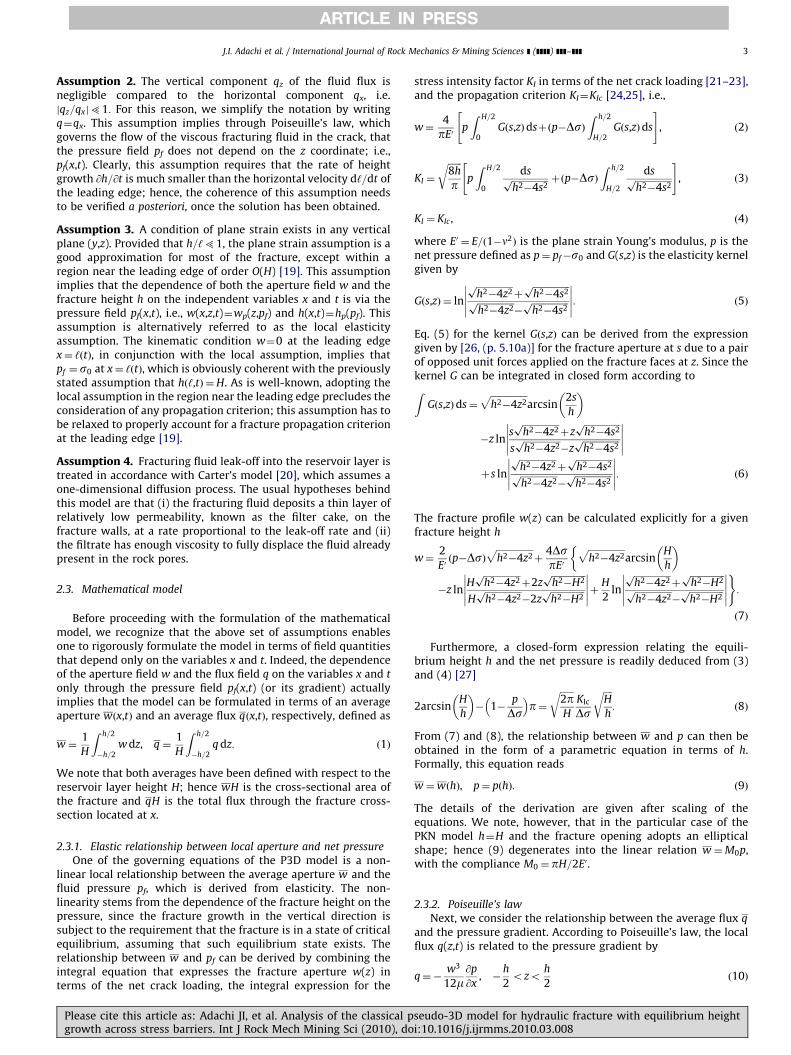
Fig. 2. Plots of w/wn versus vertical coordinate z, for different values of toughness K and equilibrium height l (l¼ 1:2, 1.4, 1.6, 1.8 and 2.0).

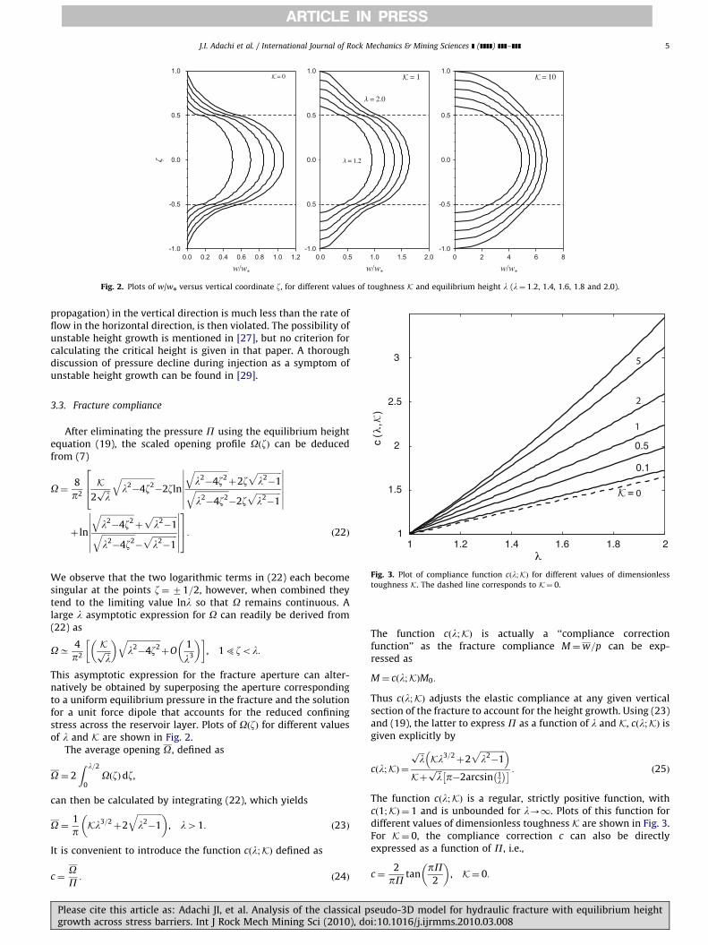
Fig. 3. Plot of compliance function cðl;KÞ for different values of dimensionless

toughness K. The dashed line corresponds to K¼ 0.

J.I. Adachi et al. / International Journal of Rock Mechanics & Mining Sciences ] (]]]]) ]]]–]]] 5

propagation) in the vertical direction is much less than the rate offlow in the horizontal direction, is then violated. The possibility ofunstable height growth is mentioned in [27], but no criterion forcalculating the critical height is given in that paper. A thoroughdiscussion of pressure decline during injection as a symptom ofunstable height growth can be found in [29].

3.3. Fracture compliance

After eliminating the pressure P using the equilibrium heightequation (19), the scaled opening profile OðzÞ can be deducedfrom (7)

O¼8

p2

K2ffiffiffilp

ffiffiffiffiffiffiffiffiffiffiffiffiffiffiffiffil2�4z2

q�2zln

ffiffiffiffiffiffiffiffiffiffiffiffiffiffiffiffil2�4z2

qþ2z

ffiffiffiffiffiffiffiffiffiffiffiffil2�1

pffiffiffiffiffiffiffiffiffiffiffiffiffiffiffiffil2�4z2

q�2z

ffiffiffiffiffiffiffiffiffiffiffiffil2�1

p�������

�������264

þ ln

ffiffiffiffiffiffiffiffiffiffiffiffiffiffiffiffil2�4z2

qþ

ffiffiffiffiffiffiffiffiffiffiffiffil2�1

pffiffiffiffiffiffiffiffiffiffiffiffiffiffiffiffil2�4z2

q�

ffiffiffiffiffiffiffiffiffiffiffiffil2�1

p�������

�������375: ð22Þ

We observe that the two logarithmic terms in (22) each becomesingular at the points z¼ 71=2, however, when combined theytend to the limiting value lnl so that O remains continuous. Alarge l asymptotic expression for O can readily be derived from(22) as

OC4

p2

Kffiffiffilp

� � ffiffiffiffiffiffiffiffiffiffiffiffiffiffiffiffil2�4z2

qþO

1

l3

� � , 15zol:

This asymptotic expression for the fracture aperture can alter-natively be obtained by superposing the aperture correspondingto a uniform equilibrium pressure in the fracture and the solutionfor a unit force dipole that accounts for the reduced confiningstress across the reservoir layer. Plots of OðzÞ for different valuesof l and K are shown in Fig. 2.

The average opening O, defined as

O ¼ 2

Z l=2

0OðzÞdz,

can then be calculated by integrating (22), which yields

O ¼1

pKl3=2

þ2

ffiffiffiffiffiffiffiffiffiffiffiffil2�1

q� �, l41: ð23Þ

It is convenient to introduce the function cðl;KÞ defined as

c¼OP: ð24Þ

Please cite this article as: Adachi JI, et al. Analysis of the classical pgrowth across stress barriers. Int J Rock Mech Mining Sci (2010), do

The function cðl;KÞ is actually a ‘‘compliance correctionfunction’’ as the fracture compliance M¼w=p can be exp-ressed as

M¼ cðl;KÞM0:

Thus cðl;KÞ adjusts the elastic compliance at any given verticalsection of the fracture to account for the height growth. Using (23)and (19), the latter to express P as a function of l and K, cðl;KÞ isgiven explicitly by

cðl;KÞ ¼

ffiffiffilpKl3=2

þ2ffiffiffiffiffiffiffiffiffiffiffiffil2�1

p� �Kþ

ffiffiffilp

p�2arcsin 1l

� � � : ð25Þ

The function cðl;KÞ is a regular, strictly positive function, withcð1;KÞ ¼ 1 and is unbounded for l-1. Plots of this function fordifferent values of dimensionless toughness K are shown in Fig. 3.For K¼ 0, the compliance correction c can also be directlyexpressed as a function of P, i.e.,

c¼2

pP tanpP2

� �, K¼ 0:

seudo-3D model for hydraulic fracture with equilibrium heighti:10.1016/j.ijrmms.2010.03.008

ARTICLE IN PRESS

Fig. 4. Plot of function UðO;KÞ for different values of dimensionless toughness K.

The dashed line corresponds to K¼ 0.

J.I. Adachi et al. / International Journal of Rock Mechanics & Mining Sciences ] (]]]]) ]]]–]]]6

Equivalently, combination of (20) and (23) allows us to derive thefollowing direct relation between O and P for K¼ 0:

p2O ¼ tan

p2P

� �, K¼ 0: ð26Þ

3.4. Viscous flow

Using the scaling (16), Poiseuille’s law (11) becomes

C ¼�gðl;KÞO3

g@P@x

, ð27Þ

where

gðl;KÞ ¼ p2

12O3

Z l=2

�l=2O3 dz: ð28Þ

The function gðl;KÞ is a regular, strictly positive function, whichasymptotically tends to zero as l-1, and liml-1þ gðl;KÞ ¼ 1;however, it cannot be expressed in a closed form. (Detailsabout the asymptotics of the function gðl;KÞ can be found inAppendix B.)

It is advantageous to express (27) as

C ¼�1

gFðl;KÞO3 @O@x

, ð29Þ

by defining the shape function F as

Fðl;KÞ ¼ g@P@l

@l@O

: ð30Þ

Using (19) and (23), the function F can be written as

Fðl;KÞ ¼ 4ffiffiffilp�K

ffiffiffiffiffiffiffiffiffiffiffiffil2�1

pl2ð4

ffiffiffilpþ3K

ffiffiffiffiffiffiffiffiffiffiffiffil2�1

pÞ

gðl;KÞ: ð31Þ

As expected, liml-1þFðl;KÞ ¼ 1. Notice that for K¼ 0, the aboveexpression reduces to

Fðl;0Þ ¼ l�2gðl;0Þ: ð32Þ

The function Fðl;KÞ eventually becomes negative as l increases,except for K¼ 0 when it tends monotonically to zero. It canreadily be shown that the function becomes negative whenlZlu; indeed both @l=@O and g are strictly positive for l41 andthus the change of sign in F simply reflects the change of sign in@P=@l, associated with the maximum value of P achieved at lu.A negative value for F actually implies a reversal of the directionof flow (i.e., the fluid would flow from the tip to the inlet—whichis unphysical for a growing fracture) in that part of the fracture forwhich l4lu, unless the gradient of opening @O=@x also reversessign, at least locally. This unphysical situation for l4lu clearlydemonstrates the limitation of the equilibrium height P3D model.

Finally the local continuity equation can be written as

1

g@C@xþ_O�x

_gg@O@xþ

Cffiffiffiffiffiffiffiffiffiffiffiffiffiffiffitð1�yÞ

p ¼ 0, ð33Þ

where yðx,tÞ ¼ t0=t is the normalized arrival time. Note that thepresence of the advective term is due to the stretching nature ofthe x�coordinate.

3.5. Scaled mathematical model

As a result of the above considerations, it is now possible toformulate the P3D model as a non-linear convection diffusionequation for the mean aperture field Oðx,tÞ and an evolutionequation for the fracture length gðtÞ.

Please cite this article as: Adachi JI, et al. Analysis of the classical pgrowth across stress barriers. Int J Rock Mech Mining Sci (2010), do

The governing equation for Oðx,tÞ is obtained by combiningPoiseuille’s law (29) and the balance law (33)

_O ¼ x_gg@O@xþ

1

g2

@

@xUðO;kÞO3 @O

@x

!�

Cffiffiffiffiffiffiffiffiffiffiffiffiffiffiffitð1�yÞ

p , ð34Þ

where the function UðO;KÞ is defined as

U¼Fð ~lðOÞ,KÞ, ð35Þ

with ~lðOÞ denoting the inverse function of (23), the relationshipbetween O and the equilibrium height l. Plots of the functionUðO;KÞ for different values of the dimensionless toughness K areshown in Fig. 4. The function UðO;KÞ is not known in closed form;however, for large O, U�O

�4if K¼ 0 and U�O

�8=3if K40, and

U¼ 1 if 0rOrOb, ð36Þ

where Ob is the critical value of the aperture at which heightgrowth starts. It is readily deduced from the equilibriumcondition (23) between l and O, which is only valid for l41 that

Ob ¼K=p: ð37Þ

Next, an equation for gðtÞ is obtained by integrating (12) inspace over the length of the fracture and then in time from theinitial time to the current time to obtain

t¼ gZ 1

0Oðx,tÞdxþ2Cg

Z 1

0

ffiffiffiffiffiffiffiffiffiffiffiffiffiffiffiffiffiffiffiffit�t0ðgxÞ

qdx: ð38Þ

The boundary conditions at the inlet ðx¼ 0Þ and at the leadingedge ðx¼ 1Þ are given by

Cð0,tÞ ¼ 1, Oð1,tÞ ¼Cð1,tÞ ¼ 0, t40: ð39Þ

Naturally, the boundary conditions in the terms of the flux Ccan be transformed to be expressed in terms of O only, using (23)and (29).

The initial condition for Oðx,tÞ is taken to correspond to a smalltime asymptotic solution when the fracture remains contained inthe reservoir layer (i.e. OrOb), and when leak-off is negligible.This similarity solution, referred to as the M-solution below, isgoverned by (34) with U¼ 1 and C¼ 0.

The system of equations (34), (38), (39), together with thesmall time asymptotic solution, constitute a closed system tosolve for the aperture field Oðx,tÞ and the fracture length gðtÞ.

seudo-3D model for hydraulic fracture with equilibrium heighti:10.1016/j.ijrmms.2010.03.008

ARTICLE IN PRESS

J.I. Adachi et al. / International Journal of Rock Mechanics & Mining Sciences ] (]]]]) ]]]–]]] 7

3.6. Tip asymptotics

We now examine the nature of the solution near the leadingedge. In the neighbourhood of the tip, the leak-off termC=

ffiffiffiffiffiffiffiffiffiffiffiffiffiffiffitð1�yÞ

pcan be approximated as

Cffiffiffiffiffiffiffiffiffiffiffiffiffiffiffitð1�yÞ

p CC

ffiffiffiffiffiffiffiffiffiffiffiffiffiffiffi_g

gð1�xÞ

s, 1�x51: ð40Þ

Using (40), the balance equation (33) is integrated in a smallregion of size e51 near the leading edgeZ 1

1�e

1

g@C@xþ_O�x

_gg@O@xþC

_ggð1�xÞ

� �1=2" #

dx¼ 0, ð41Þ

which, after taking into account the boundary conditionsC ¼O ¼ 0 at x¼ 1, implies that

C �x-1

_gOþ2Cffiffiffiffiffiffiffiffiffiffiffiffiffiffiffiffiffiffig _gð1�xÞ

q: ð42Þ

Combining (42) with Poiseuille’s law (29) then yields

O3

g@O@xþ _gOþ2C

ffiffiffiffiffiffiffiffiffiffiffiffiffiffiffiffiffiffig _gð1�xÞ

q�

x-10, ð43Þ

where we have taken into account that F� 1 as x-1.In the two limiting cases of storage- and leak-off-dominated

asymptotics, the behaviour of O near the leading edge can bededuced from (43), by adopting an asymptotic solution for O ofthe form

O �x-1

AðtÞð1�xÞa: ð44Þ

In the storage-dominated case, the first two terms in (43) have tobalance; hence

a¼ 1

3, A¼

ffiffiffiffiffiffiffiffiffi3 _gg3

p: ð45Þ

In the leak-off-dominated case, however, the first and third termin (43) have to balance; hence the power law index a and thestrength A are given by

a¼ 3

8, A¼

2

31=4ð _gg3C2Þ

1=8: ð46Þ

The tip asymptotic behaviour in between these two limiting casescan also be obtained, see [30] for more details. However, apragmatic approach is to adopt (45) when gogc (or totcÞ and(46) when gZgc (or tZtcÞ where

gc ¼g8=3~m0

g5=3m0

tc ¼g ~m0

gm0

� �10=3

, ð47Þ

with gm0 and g ~m0ðCÞ, two numbers that are related to theasymptotics of the fracture length for a PKN fracture at smalland large time, i.e. when the contained fracture propagates in thestorage- and leak-off-dominated regime, respectively (see (48)and (49)). The length gc corresponds to the intersection of thesmall and large time asymptotic solutions for the length of a PKNfracture, while tc is the time corresponding to the intersection ofthese two asymptotes. In the MATLAB code colP3D [31] thatimplements the algorithm presented in this paper, the switchbetween the two tip asymptotes is based on the time criterion.This approach (based on either the length or the time criterion) isempirically justified by the observations, reported further in thispaper, that the evolution of the fracture length is influenced littleby the height growth. An alternative empirical approach would beto switch from (45) to (46) for the tip asymptote, when the tipvelocity decreases below a critical value deduced from comparingthe small and large time asymptotics for the tip velocity of acontained fracture.

Please cite this article as: Adachi JI, et al. Analysis of the classical pgrowth across stress barriers. Int J Rock Mech Mining Sci (2010), do

4. Regimes of solution

4.1. Time scales and similarity solutions

The P3D fracture problem is governed by two time scales, onelegislating the height growth and the other characterizing thetransition from a storage-dominated to a leak-off-dominatedregime.

The characteristic time tn introduced earlier does not dependon the toughness KIc of the adjacent layers, nor on the leak-offcoefficient C0 of the reservoir layer. It actually represents the timescale needed to reach, under the particular conditions C¼K¼ 0, alarge time similarity solution characterized by g¼ Const: andO � t on account that U�O

�4when tb1. Unfortunately, this

similarity solution violates the basic assumption on which theP3D model is based, namely that the flow is mainly horizontal(i.e. longitudinal), and is therefore only a mathematical curiositydevoid of any physical interest. Nonetheless, tn represents a scalefor the time required to reach this height growth dominatedsimilarity solution.

Under conditions when the fracture remains confined to thereservoir ðl¼ 1Þ, the time scale C�10=3t� characterizes the transi-tion between a regime where the injected fluid is essentiallyoccupying the fracture to a regime where most of the fluid leaksinto the reservoir. Both regimes are described by similaritysolutions with a power law dependence on time [30], seeAppendix A for further details.The M-solution (storage-dominated regime):

Oðx,tÞ ¼Om0ðxÞt1=5, gðtÞ ¼ gm0t4=5, ð48Þ

with gm0C1:006 and Om0ð0ÞC1:326.The ~M-solution (leak-off-dominated regime):

Oðx,tÞ ¼O ~m0ðx,CÞt1=8, gðtÞ ¼ g ~m0ðCÞt1=2, ð49Þ

with g ~m0 ¼ 2=pC and O ~m0ð0Þ ¼ 2=p1=2C1=4.Thus the transition between the early-time M-solution and the

large-time ~M-solution evolves with the dimensionless time C10=3t.Calculations with the PKN model show, with an error of about 2%or less, that the confined fracture grows in the storage-dominatedregime if C10=3tt10�5 and in the leak-off-dominated regime ifC10=3t\103 [30]. Reaching the ~M-solution requires K to be largeenough (actually at least of order Oð10C�2=3

Þ) to ensure contain-ment of the fracture within the reservoir layer.

The M-solution is of particular importance because it serves asa small time asymptotic solution from which the P3D fractureevolves. While other processes may have taken place at timesprior to those at which the M-solution is applicable (for example,when the fracture length is smaller than or of the same order asthe reservoir thickness H), the existence of an intermediate timesimilarity solution usually implies that the details of the earlierfracture evolution do not affect the process anymore once thesimilarity solution develops [32]. This means that the evolution ofthe P3D fracture can effectively start from the M-solution, andthat the prior history can be ignored. However, as shown below,the M-solution is an appropriate small time asymptotic solutionfor the P3D fracture, only if the dimensionless toughness K40.

4.2. Phases in fracture height growth

In principle, we can identify four phases of height growthduring propagation of the P3D hydraulic fracture, which aredelimited by three time markers: (i) the breakthrough time tb

corresponding to the onset of height growth, (ii) tp when thefracture has penetrated into the layers bounding the reservoir

seudo-3D model for hydraulic fracture with equilibrium heighti:10.1016/j.ijrmms.2010.03.008

ARTICLE IN PRESS

Fig. 5. Contour lines of the breakthrough time tb in the ðC,KÞ space.

J.I. Adachi et al. / International Journal of Rock Mechanics & Mining Sciences ] (]]]]) ]]]–]]]8

layers throughout its length, and (iii) tu when height growthbecomes unstable.Phase 1: Complete fracture containment (lðx,tÞ ¼ 1 for 0rxr1 and

trtbðC,KÞ). The fracture opening O is everywhere less than thethreshold value Ob ¼K=p given by (37). During this phase, thefracture behaves according to the PKN solution [9,30].Phase 2: Partial fracture containment (lðx,tÞ41 for 0rxoxlðtÞ and

lðx,tÞ ¼ 1 for xlðtÞrxr1; tbðC,KÞrtrtpðC,KÞ). At the interface,Oðxl,tÞ ¼Ob and lðxl,tÞ ¼ 1. The position xlðtÞ of the interfacebetween the contained and uncontained fracture regions in-creases with time, with xlðtbÞ ¼ 0 and xlðtpÞ ¼ 1: In the limit K¼ 0,the fracture is never contained, i.e. tb ¼ tp ¼ 0.Phase 3: No fracture containment (lðx,tÞ41 for 0rxo1 and

tpðC,KÞrtrtuðC,KÞ). The fracture opening O is larger than ObðKÞthroughout 0rxrxlðtÞ but less than OuðKÞ at which value theheight growth becomes unstable.Phase 4: Unstable height growth (lð1,tÞ4luðKÞ for tZtuðC,KÞ). Thesolution loses its physical meaning once the height growthbecomes unstable, which corresponds to the condition O ¼Ou,given by

Ou ¼1

pK216þ

ffiffiffiffiffiffiffiffiffiffiffiffiffiffiffiffiffiK4þ64

q� � ffiffiffiffiffiffiffiffiffiffiffiffiffiffiffiffiffiffiffiffiffiffiffiffiffiffiffiffiffi8þ

ffiffiffiffiffiffiffiffiffiffiffiffiffiffiffiffiffiK4þ64

qr: ð50Þ

Since O is a monotonically decreasing function, i.e., @O=@xo0 of x(otherwise the fluid flow would be reversed), the runawaycondition will first be reached at the inlet. Hence the time tu atwhich the instability takes place corresponds to Oð0,tuÞ ¼Ou. Theonset of unstable height growth marks the end of applicability ofthe equilibrium height P3D model, but the beginning of relevanceof the dynamic height model.

Unlike the calculations of tp and tu, which require solving thefull set of equations governing the evolution of the P3D fracture,the breakthrough time tbðC,KÞ can be readily calculated from theknown contained (PKN) fracture solution. The evolution of thefracture aperture at the wellbore O0ðtÞ ¼Oð0,tÞ can be deducedfrom the PKN solution to be of the form [30]

O0ðt; C,KÞ ¼2

C

� �2=3

O0�C10=3

24=3t

!, ð51Þ

where the function O0�ðt�Þ is the inlet opening in the PKN scaling[30]. Since the fracture starts to grow into the confining layerswhen the mean fracture aperture at the borehole reaches thethreshold ObðKÞ, the breakthrough time tb is deduced to be givenby

tb ¼24=3

C10=3O�1

0�

C2=3K22=3p

!ð52Þ

where O�1

0� denotes the inverse function of O0�. From the knownsmall and large time asymptotics of O0�, the asymptotics of tb forsmall and large C2=3K can readily be deduced.Storage-dominated asymptote:

tbs ¼K

pOm0ð0Þ

!5

C0:79710�3K5, C2=3Kt0:66: ð53Þ

Leak-off-dominated asymptote:

tbl ¼C2K8

28p4, C2=3K\8:5 ð54Þ

The above expression for tbs shows that the M-solution is notthe appropriate early-time solution for the P3D geometry, if K¼ 0.However, we still use the M-solution to initialize the calculationsin that case since the correct early time solution has not yet beenestablished.

Contour plots of the breakthrough time tbðC,KÞ in the spaceðC,KÞ are shown in Fig. 5.

Please cite this article as: Adachi JI, et al. Analysis of the classical pgrowth across stress barriers. Int J Rock Mech Mining Sci (2010), do

5. Numerical algorithm

5.1. A fourth order collocation scheme to solve the model equations

In this section we describe a fourth order collocation schemeto solve the two-point boundary value problem (34) along withthe boundary conditions (39). In order to express the modelequations as a first order system over the domain xAð0,1Þ, werevert to Poiseuille’s law and the original conservation law, whichcan be expressed in the form

@O@x¼�

gC

UðO;KÞO3¼ F1ðx;O,C,gÞ, ð55Þ

@C@x¼�

xg _gC

UðO;KÞO3�g _O� Cffiffiffiffiffiffiffiffiffiffiffiffiffiffiffiffiffiffiffiffi

t�t0ðgxÞp ¼ F2ðx;O,C,gÞ: ð56Þ

Eq. (38) for gðtÞ, expressing global conservation of the fracturingfluid, i.e.,

t¼ gZ 1

0Oðx,tÞdxþ2Cg

Z 1

0

ffiffiffiffiffiffiffiffiffiffiffiffiffiffiffiffiffiffiffiffit�t0ðgxÞ

qdx ð57Þ

completes the system of equations. The time derivatives in (55)and (56) are replaced by the following backward differenceapproximations:

_gC gt�gt�DtDt and _OC

Ot�Ot�DtDt : ð58Þ

With these difference approximations, (55) and (56) are reducedto a system of ordinary differential equations for O and C, which,when combined with (57), form a nonlinear system that issufficient to determine ðO,C,gÞ at time t given the values at t�Dt.This time stepping strategy can be interpreted as the backwardEuler approximation to the time derivatives in a method of linesscheme in which the spatial discretization has yet to be defined.The inlet boundary condition Cð0,tÞ ¼ 1 is imposed at the leftendpoint of the domain. At the right endpoint of the domain x¼ 1,corresponding to the fracture tip, we have seen from ourasymptotic analysis that O � AðtÞð1�xÞa, where 0oao1. Thuspolynomial approximations to O, which include the tip, would beinaccurate due to the fact that the derivatives of O are singular.For this reason we decompose the interval [0,1] as follows½0,1� ¼ ½0,xc� [ ðxc ,1� into a channel region ½0,xc� and a tip regionðxc ,1�. In the channel region we apply a collocation approximation

seudo-3D model for hydraulic fracture with equilibrium heighti:10.1016/j.ijrmms.2010.03.008

ARTICLE IN PRESS

Fig. 6. Comparison between computed gðtÞ and Oð0,tÞ for imposed l¼ 1 (PKN

solution) with small and large time asymptotics (calculation performed for C¼ 1).

J.I. Adachi et al. / International Journal of Rock Mechanics & Mining Sciences ] (]]]]) ]]]–]]] 9

to (55) and (56) and use a consistent approximation for theintegrals in (57). The right boundary condition for this system ofODE is then provided by the appropriate tip asymptotic solution(44) evaluated at xc , while the remaining contributions from thetip region to the integrals in (57) are determined by the tipasymptotics. In particular, assuming the asymptotic behavior (44)we obtain the following approximation for the storage integralover the tip region:Z 1

xc

Oðx,tÞdxC AðtÞ1þa ð1�xcÞ

1það59Þ

and we make the following approximation to the leak-off integralover the tip region:Z 1

xc

ffiffiffiffiffiffiffiffiffiffiffiffiffiffiffiffiffiffiffiffit�t0ðgxÞ

qdxC

Z 1

xc

ffiffiffiffiffiffiffiffiffiffiffiffiffiffiffiffig_gð1�xÞ

rdx¼

g_g

� �1=2 2

3ð1�xcÞ

3=2: ð60Þ

In order to discretize the nonlinear system (55) and (56), theinterval ½0,xc� is partitioned into n�1 subintervals with break-points f0¼ x1,x2, . . . ,xn�1,xn ¼ xcg. Defining the vector Y ¼ ðO,CÞwe can re-write the system of equations (55) and (56) in thefollowing compact form:

dY

dx¼ Fðx;Y ,gÞ, ð61Þ

where g is regarded as a parameter and the components of thegradient field Fðx;Y ,gÞ are defined in (55) and (56). Following theapproximation scheme adopted in [33], we assume a Hermitecubic approximation to Y on each subinterval. Integrating (61)over a typical subinterval ½xk,xkþ1�, we obtain an integral form of(61), which we then approximate using Simpson’s Rule

Ykþ1 ¼ Ykþ

Z xkþ 1

xk

Fðx;YðxÞ,gÞdx

¼ YkþDx6

Fkþ1þ4Fkþ 12þFk

h iþOðDx5

Þ:

As in [33] we use the following Hermite cubic approximant to~Y kþ1=2 ¼ ðYkþYkþ1Þ=2�ðDx=8ÞðFkþ1�FkÞ to evaluate Fkþ1=2CFðxkþ1=2, ~Y kþ1=2Þ in the Simpson approximation. Consistent withthe above approximation, we use the Composite Simpson’s Ruleto approximate the storage and leak-off integrals over the channelregion.

The above discretizations reduce the continuous system(55)–(57) to a system of 2n�1 nonlinear equations for the 2n+1unknowns fO1, . . . ,On;C1, . . . ,Cn; gg. The two boundary condi-tions C1 ¼ 1 and On ¼OtipðxcÞ provide the additional constraintsrequired to solve for the 2n+1 unknowns. The complete system ofnonlinear equations is solved at each time step using a Newtoniteration scheme in which a finite difference approximation isused to evaluate the Jacobian for the system at each iteration.

5.2. Accuracy and robustness of the algorithm

The spatial discretization used in the numerical scheme has aglobal truncation error of OðDx4

Þ, see [33], while the backwarddifference formula used to approximate the time derivatives has atruncation error of OðDtÞ. To match the spatial to time scalingx=

ffiffiffitp

, which is intrinsic to diffusion problems, it might bedesirable to use a second order backward difference approxima-tion to achieve a truncation order OðDx4,Dt2Þ. However, we havechosen not to do this in order to maintain the simplicity andbrevity of the code which can be downloaded [31]. For this classof problems an explicit time stepping scheme would require a CFLcondition of the form DtrkDx2, necessitating extremely smalltime steps and long run times. Since the implicit backwarddifference time stepping scheme used in this algorithm is anL-stable method there is no time step restriction. In order to

Please cite this article as: Adachi JI, et al. Analysis of the classical pgrowth across stress barriers. Int J Rock Mech Mining Sci (2010), do

perform simulations that connect both small and large timescales, we have found that increasing the size of the time step by ageometric factor r41, i.e., Dtkþ1 ¼ rDtk at each time step to be asuccessful approach. For the results presented in the next section,we have chosen a conservative approach for the choice of thegeometric time factor r¼1.01 in order to reduce the OðDtÞtruncation errors to a minimum. For the problems in which weexplore the penetration of the layers, we have also chosen arelatively fine spatial mesh n¼60 in order to be able to capturethe evolving penetration boundary l¼ 1 with greater resolution.However, substantially larger r42 factors are possible withoutadversely affecting the results and, as the comparisons with thePKN asymptotic solutions demonstrate, a coarse mesh comprisingjust n¼10 collocation points yields results that are almostindistinguishable from the asymptotic solutions.

6. Numerical simulations

In this section, we report results of a series of numericalsimulations carried out with the MATLAB code colP3D [31] thatimplements the algorithm described above. First, we validate thealgorithm by comparing the results of the simulations with theknown small and large time asymptotic solutions under condi-tions when height growth is prohibited. Second, we perform aseries of simulations in which height growth is allowed and forwhich the leak-off and toughness parameters, C and K, assumeone of the values 0 or 1.

6.1. Simulation without height growth (PKN)

To validate the numerical algorithm, we conducted a simula-tion by forcing the fracture to remain contained within thereservoir layer (i.e., lðx,tÞ ¼ 1), which formally corresponds to thelimiting case K¼1. Although the dimensionless leak-off coeffi-cient C can be absorbed through a rescaling of the equations inthis particular case, by redefining the characteristic time, length,and width (see Appendix A), the calculations were nonethelessperformed on the basis of the originally scaled equations for C¼ 1.The discretization parameters for the simulation were n¼10 andr¼1.2. The calculations were started at t¼ 10�8 with an initialtime step Dt¼ 10�9, and ended at t¼ 105, so as to guarantee thatthe computed solution indeed evolves from the small time to thelarge time similarity solution.

seudo-3D model for hydraulic fracture with equilibrium heighti:10.1016/j.ijrmms.2010.03.008

ARTICLE IN PRESS

J.I. Adachi et al. / International Journal of Rock Mechanics & Mining Sciences ] (]]]]) ]]]–]]]10

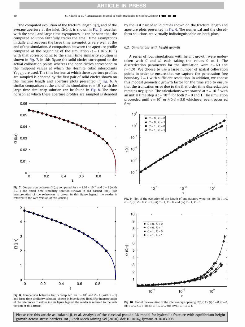
The computed evolution of the fracture length, gðtÞ, and of theaverage aperture at the inlet, Oð0,tÞ, is shown in Fig. 6, togetherwith the small and large time asymptotes. It can be seen that thecomputed solution faithfully tracks the small time asymptoticsinitially and recovers the large time asymptotics very well at theend of the simulation. A comparison between the aperture profilecomputed at the beginning of the simulation ðt¼ 1:16� 10�7

Þ

with that corresponding to the small time similarity solution isshown in Fig. 7. In this figure the solid circles correspond to theactual collocation points whereas the open circles correspond tothe midpoint values at which the Hermite cubic interpolants~Y kþ1=2 are used. The time horizon at which these aperture profilesare sampled is denoted by the first pair of solid circles shown onthe fracture length and aperture plots presented in Fig. 6. Asimilar comparison at the end of the simulation ðt¼ 105

Þ with thelarge time similarity solution can be found in Fig. 8. The timehorizon at which these aperture profiles are sampled is denoted

Fig. 7. Comparison between Oðx,tÞ computed for t¼ 1:16� 10�7 and C¼ 1 (with

l¼ 1) and small time similarity solution (shown in red dashed line). (For

interpretation of the references to colour in this figure legend, the reader is

referred to the web version of this article.)

Fig. 8. Comparison between Oðx,tÞ computed for t¼ 105 and C¼ 1 (with l¼ 1)

and large time similarity solution (shown in blue dashed line). (For interpretation

of the references to colour in this figure legend, the reader is referred to the web

version of this article.)

Please cite this article as: Adachi JI, et al. Analysis of the classical pgrowth across stress barriers. Int J Rock Mech Mining Sci (2010), do

by the last pair of solid circles shown on the fracture length andaperture plots presented in Fig. 6. The numerical and the closed-form solutions are virtually indistinguishable on both plots.

6.2. Simulations with height growth

A series of four simulations with height growth were under-taken with C and K, each taking the values 0 or 1. Thediscretization parameters for the simulation were n¼60 andr¼1.01. We choose to use a large number of spatial collocationpoints in order to ensure that we capture the penetration freeboundary l¼ 1 with sufficient resolution. In addition, we choosethis modest geometric growth factor for the time step to ensurethat the truncation error due to the first order time discretizationremains negligible. The calculations were started at t¼ 10�8 withan initial time step Dt¼ 10�9 for both C¼ 0 and 1. The simulationproceeded until t¼ 102 or lð0,tÞ ¼ 5:0 whichever event occurredfirst.

Fig. 9. Plot of the evolution of the length of one fracture wing gðtÞ for (i) C¼ 0,

K¼ 0, (ii) C¼ 0, K¼ 1, (iii) C¼ 1, K¼ 0, and (iv) C¼ 1, K¼ 1.

Fig. 10. Plot of the evolution of the inlet average opening Oð0,tÞ for (i) C¼ 0, K¼ 0,

(ii) C¼ 0, K¼ 1, (iii) C¼ 1, K¼ 0, and (iv) C¼ 1, K¼ 1.

seudo-3D model for hydraulic fracture with equilibrium heighti:10.1016/j.ijrmms.2010.03.008

ARTICLE IN PRESS

J.I. Adachi et al. / International Journal of Rock Mechanics & Mining Sciences ] (]]]]) ]]]–]]] 11

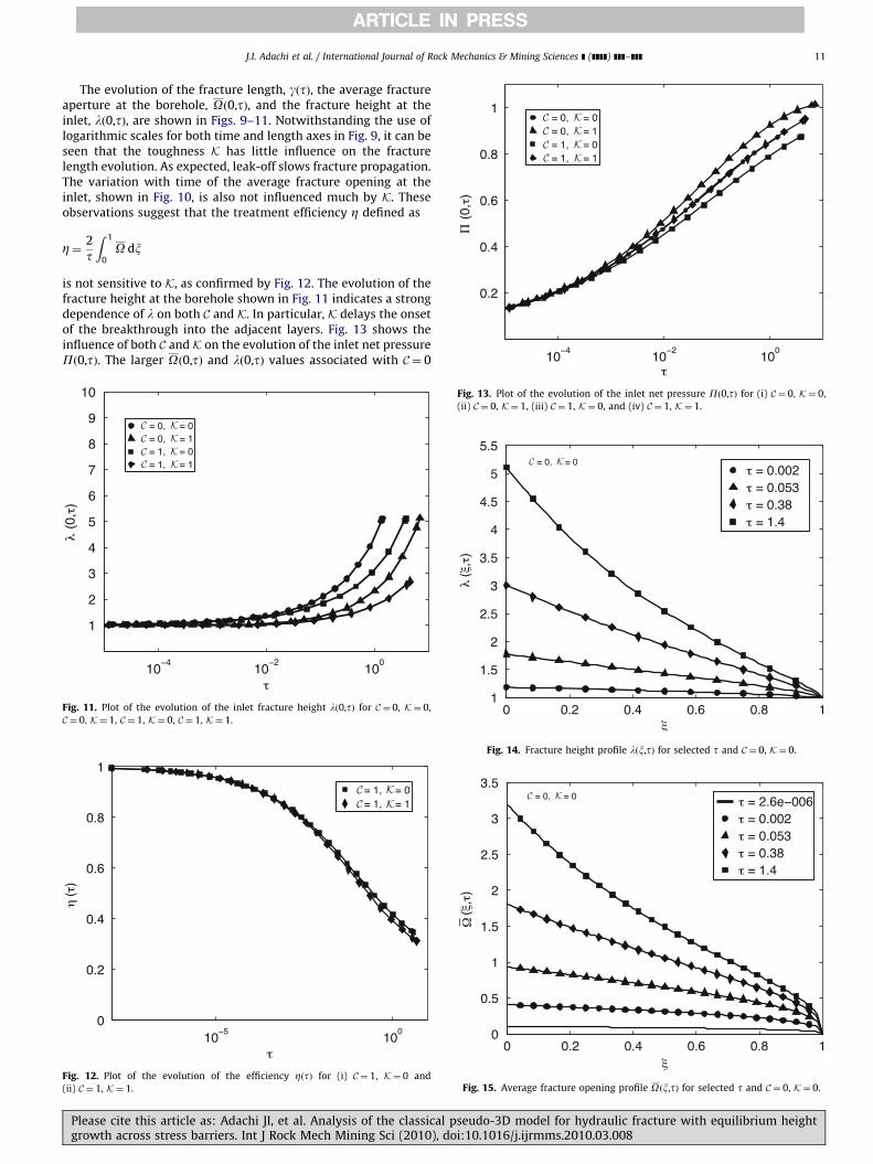
The evolution of the fracture length, gðtÞ, the average fractureaperture at the borehole, Oð0,tÞ, and the fracture height at theinlet, lð0,tÞ, are shown in Figs. 9–11. Notwithstanding the use oflogarithmic scales for both time and length axes in Fig. 9, it can beseen that the toughness K has little influence on the fracturelength evolution. As expected, leak-off slows fracture propagation.The variation with time of the average fracture opening at theinlet, shown in Fig. 10, is also not influenced much by K. Theseobservations suggest that the treatment efficiency Z defined as

Z¼ 2

t

Z 1

0O dx

is not sensitive to K, as confirmed by Fig. 12. The evolution of thefracture height at the borehole shown in Fig. 11 indicates a strongdependence of l on both C and K. In particular, K delays the onsetof the breakthrough into the adjacent layers. Fig. 13 shows theinfluence of both C and K on the evolution of the inlet net pressurePð0,tÞ. The larger Oð0,tÞ and lð0,tÞ values associated with C¼ 0

Fig. 11. Plot of the evolution of the inlet fracture height lð0,tÞ for C¼ 0, K¼ 0,

C¼ 0, K¼ 1, C¼ 1, K¼ 0, C¼ 1, K¼ 1.

Fig. 12. Plot of the evolution of the efficiency ZðtÞ for (i) C¼ 1, K¼ 0 and

(ii) C¼ 1, K¼ 1.

Fig. 13. Plot of the evolution of the inlet net pressure Pð0,tÞ for (i) C¼ 0, K¼ 0,

(ii) C¼ 0, K¼ 1, (iii) C¼ 1, K¼ 0, and (iv) C¼ 1, K¼ 1.

Fig. 14. Fracture height profile lðx,tÞ for selected t and C¼ 0, K¼ 0.

Fig. 15. Average fracture opening profile Oðx,tÞ for selected t and C¼ 0, K¼ 0.

Please cite this article as: Adachi JI, et al. Analysis of the classical pseudo-3D model for hydraulic fracture with equilibrium heightgrowth across stress barriers. Int J Rock Mech Mining Sci (2010), doi:10.1016/j.ijrmms.2010.03.008

ARTICLE IN PRESS

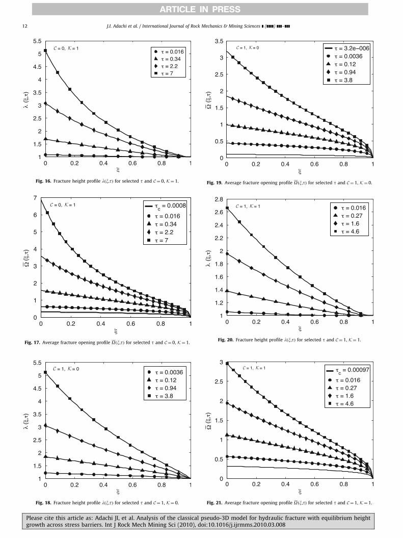
Fig. 16. Fracture height profile lðx,tÞ for selected t and C¼ 0, K¼ 1.

Fig. 17. Average fracture opening profile Oðx,tÞ for selected t and C¼ 0, K¼ 1.

Fig. 18. Fracture height profile lðx,tÞ for selected t and C¼ 1, K¼ 0.

Fig. 19. Average fracture opening profile Oðx,tÞ for selected t and C¼ 1, K¼ 0.

Fig. 20. Fracture height profile lðx,tÞ for selected t and C¼ 1, K¼ 1.

Fig. 21. Average fracture opening profile Oðx,tÞ for selected t and C¼ 1, K¼ 1.

J.I. Adachi et al. / International Journal of Rock Mechanics & Mining Sciences ] (]]]]) ]]]–]]]12

Please cite this article as: Adachi JI, et al. Analysis of the classical pseudo-3D model for hydraulic fracture with equilibrium heightgrowth across stress barriers. Int J Rock Mech Mining Sci (2010), doi:10.1016/j.ijrmms.2010.03.008

ARTICLE IN PRESS

J.I. Adachi et al. / International Journal of Rock Mechanics & Mining Sciences ] (]]]]) ]]]–]]] 13

and K¼ 0 seem to yield the same Pð0,tÞ values as the muchsmaller Oð0,tÞ and lð0,tÞ values associated with the case C¼ 1 andK¼ 1. These simulations imply therefore that the fracture length,mean fracture opening, and efficiency are mainly affected by theleak-off coefficient C. The toughness K essentially impacts thevertical growth of the fracture, the maximum fracture aperture,and the fracture pressure.

Figs. 14–21 display the fracture height profile lðx,t) andopening profile Oðx,tÞ at selected times for the four casesconsidered. The opening profiles at the time of breakthrough, tb,for K¼ 1 (or at the start of the simulation for K¼ 0) arerepresented by continuous lines without symbols in thesefigures. These profiles demonstrate the dramatic influence of thefracture height growth on the shape of the fracture openingprofile.

7. Conclusions

In this paper we have revisited the classical equilibrium height‘‘Pseudo-3D’’ model of a hydraulic fracture, which is used in thedesign of most hydraulic fracturing treatments. This model,introduced in the early 1980s by a number of researchers as anextension of the PKN model, allows for penetration of the fractureinto the layers bounding the hydrocarbon reservoirs, whilemaintaining all the other simplifying assumptions on which thePKN model is built. The paper takes a different tack from previouscontributions on the P3D model. Rather than following ab initio adiscrete formalism, it first adopts a continuous formulation andscaling of the problem, thus allowing for further analysis of themathematical model before embarking on the development of anumerical algorithm. This approach leads to a nonlinear convec-tion diffusion equation with a delay term that governs the meanfracture aperture O, supplemented by an integral condition to besolved for the fracture length g.

In this novel formulation of the P3D model, the effect of theheight growth is entirely embodied in the function UðOÞFasource of additional non-linearity in the P3D model comparedwith the PKN model, as this function is simply unity if the fractureremains confined to the reservoir. The function UðOÞ captures thevariation of the hydraulic conductivity associated with penetra-tion of the fracture into the adjacent layers, while implicitlyaccounting for the propagation criterion that controls its verticalgrowth. Although the paper restricts consideration to the simplebut important case of identical elastic properties for the reservoir,with impermeable bounding layers and symmetric stress barriers,the formulation used is general. Other factors influencing fractureheight growth, such as multiple bounding layers with differentelastic properties and confining stresses, can simply be assimi-lated in the function UðOÞ, which is in principle computable. Evenfor the simple configuration of concern here, the function UðOÞ isnot known in closed form. However, its dependence on onenumber only, the scaled toughness K of the bounding layers,ensures that it can easily be pretabulated. Furthermore, thecondition of unstable height growth, which marks the limit ofvalidity of one of the key assumptions of the P3D model, namelythe vertical uniformity of the fluid pressure, can be determinedexplicitly in the form of a simple upper bound OuðKÞ on O.

Another contribution reported in this paper is the develop-ment of an implicit fourth order collocation scheme on a movingmesh to solve the nonlinear partial differential equations and theintegral relation governing the response of the P3D model. Thenumerical method, which approximates both the mean fractureopening O and the mean flux C by a cubic polynomial over adiscretization interval, is fourth order accurate in the spacevariable. Despite being first order accurate in time, a doubling of

Please cite this article as: Adachi JI, et al. Analysis of the classical pgrowth across stress barriers. Int J Rock Mech Mining Sci (2010), do

the size of the time step at each new step still leads to accurateresults while permitting a very rapid simulation over manytemporal orders of magnitude. The fourth order spatial approx-imation numerical scheme implies that the solution could satis-factorily be captured using a rather coarse mesh. However, theaccurate tracking of the penetration front ðl¼ 1Þ during thepropagation phase, when the fracture is partially contained,requires sufficient spatial resolution of the computational grid.Nonetheless, this algorithm could, in principle, be improved byexplicitly recognizing the existence of a propagation front,through the introduction of two moving meshes: one for thecontained region and one for the uncontained region.

Finally, an analysis of the behavior of the P3D model wasconducted through a series of numerical simulations. Actually, anassessment of the overall behavior of the system can readily bemade, as only two numbers, K and C, control the solution—thanksto the assumption of symmetric stress barriers, homogeneouselastic properties, and constant injection rate adopted for thisstudy. In particular, the limits of the four regimes of propagationof a P3D fracture (fully, partially, and not contained to thereservoir layer, as well as unstable height growth) can beexpressed simply in terms of time thresholds that only dependon K and C. Also, as realistic values of the physical parameterstypically correspond to values of K and C within the range [0,1],we reported the results of four simulations conducted for eachcombination of K and C taking values of 0 or 1 so as to provideglimpse of expected variation in the response of the system.Remarkably, we found that the mean aperture field Oðx,t) and thefracture length gðtÞ do not deviate significantly from theprediction of the PKN model. However, since the fracturecompliance c is sensitive to the actual height of the fracture, thenet pressure is strongly influenced by penetration of the fractureinto the bounding layers.

The rigorous mathematical formulation of the P3D modelpresented in this paper has made it possible to clearly identify theimportant regimes of propagation from a contained fractureinitiating in the storage regime to a final state comprising apartially or fully penetrated fracture propagating in the leak-offdominated regime. A clear criterion for the onset of runawayheight growth, beyond which the model fails to be valid, hasalso been established. The scaling analysis has made it possibleto clearly establish the fundamental relationship betweenthe front propagation dynamics and the propagation regimesof the classical PKN model and the P3D model. The novelimplicit spatially fourth order collocation scheme is shown to berobust and makes it possible to accurately explore the behaviorof the solution over the large range of time scales active in theproblem. The algorithm implemented in the downloadableMATLAB code colP3D [31] could in principle be extended toaccount for power law fluids, proppant transport, variableinjection rate and multiple layers. Such extensions would makeit a useful design code for Industry.

Acknowledgements

J.I.A. would like to Schlumberger for permission to publish.E. Detournay gratefully acknowledges support from the NationalScience Foundation under Grant no. 0600058; however, anyopinions, findings, and conclusions or recommendations ex-pressed in this material are those of the authors and do notnecessarily reflect the views of the National Science Foundation.Finally, A. Peirce acknowledges the support of the NSERCdiscovery grants program.

seudo-3D model for hydraulic fracture with equilibrium heighti:10.1016/j.ijrmms.2010.03.008

ARTICLE IN PRESS

J.I. Adachi et al. / International Journal of Rock Mechanics & Mining Sciences ] (]]]]) ]]]–]]]14

Appendix A. Similarity solutions for contained (PKN)hydraulic fractures

The solution of the contained hydraulic fracture is well-known[9,34,30]. The quantities can be scaled in such a way that thesolution does not depend on any parameters other than thestretching coordinate x and a dimensionless time t� [30].The relationship between the scaled quantities introduced inthis paper and those defined by [30] (denoted by an asterisk) aregiven by

O ¼2

C

� �2=3

O�, g¼ 25

C8

!1=3

g�, t¼ 24

C10

!1=3

t�: ðA:1Þ

The solution degenerates into a similarity solution at small time(the M-solution) ðt�t10�4

Þ and at large time (the M~-solution)ðt�\102

Þ, both characterized by a power law dependence ontime.M-solution. The small time asymptotic solution behaves with timeaccording to

gðtÞ ¼ gm0t4=5, Oðx,tÞ ¼Om0ðxÞt1=5, t51, ðA:2Þ

with Om0ðxÞ and gm0 governed by

5

4g2m0

d2O4

m0

dx2þ4x

dOm0

dx�Om0 ¼ 0, 2gm0

Z 1

0Om0 dx¼ 1, Om0ð1Þ ¼ 0:

ðA:3Þ

The solution of (A.3) yields

Om0 ¼12

5

� �1=3

g2=3m0 ð1�xÞ

1=3 1�1

96ð1�xÞ

� �þOðð1�xÞ7=3

Þ, ðA:4Þ

and gm0C1:00063.~M-solution. The large time asymptotic solution behaves with time

according to

gðtÞ ¼ g ~m0t1=2, Oðx,tÞ ¼O ~m0ðxÞt1=8, tb1, ðA:5Þ

with O ~m0ðxÞ and g ~m0 governed by

d2O4~m0

dx2�

4Cg4~m0ffiffiffiffiffiffiffiffiffiffiffiffi

1�x2q ¼ 0, 2Cg ~m0

Z 1

0

ffiffiffiffiffiffiffiffiffiffiffiffi1�x2

qdx¼ 1: ðA:6Þ

The solution of (A.6) yields

O ~m0ðxÞ ¼8

pC

� �1=4 2

pxarcsinxþ

2

p

ffiffiffiffiffiffiffiffiffiffiffiffi1�x2

q�x

� �1=4

, g ~m0 ¼2

pC :

ðA:7Þ

The series expansion of O ~m0ðxÞ with respect to the tip is given by

O ~m0ðxÞ ¼211=8

p1=2ð3CÞ1=4ð1�xÞ3=8 1þ

1

80ð1�xÞ

� �þOðð1�xÞ19=8

Þ:

ðA:8Þ

Appendix B. Asymptotics of the function gðl,KÞ

It is possible to extract some information about the asymptoticbehaviors of the function gðl,KÞ. We first rewrite the apertureOðz;K,lÞ in terms of the space variable u¼ 2z=l, i.e.~Oð2z=l;K,lÞ ¼Oðz;K,lÞ and express ~O into two contributions,

one that is independent of K and another one that is proportionalto K. Furthermore, since the aperture is symmetric with respect tou¼0, we are only concerned here with u40

~O ¼ ~O0ðu;lÞþKl1=2 ~OkðuÞ, 0rur1, ðB:1Þ

Please cite this article as: Adachi JI, et al. Analysis of the classical pgrowth across stress barriers. Int J Rock Mech Mining Sci (2010), do

where

~Oo ¼8

p2~f2 ðu; lÞ�ul ~f1 ðu; lÞ

h i, ~Ok ¼

4

p2

ffiffiffiffiffiffiffiffiffiffiffiffi1�u2

p, ðB:2Þ

with

f1ðu; lÞ ¼

arctanhu

ffiffiffiffiffiffiffiffiffiffiffiffil2�1

pffiffiffiffiffiffiffiffiffiffiffiffi1�u2p

!, 0ruo

1

l,

arctanh

ffiffiffiffiffiffiffiffiffiffiffiffi1�u2p

uffiffiffiffiffiffiffiffiffiffiffiffil2�1

p !

,1

lour1,

8>>>>><>>>>>:

f2ðu; lÞ ¼

arctanh

ffiffiffiffiffiffiffiffiffiffiffiffil2�1

plffiffiffiffiffiffiffiffiffiffiffiffi1�u2p

!, 0ruo

1

l,

arctanhlffiffiffiffiffiffiffiffiffiffiffiffi1�u2p

ffiffiffiffiffiffiffiffiffiffiffiffil2�1

p !

,1

lour1:

8>>>>><>>>>>:

ðB:3Þ

B.1. Large penetration asymptote

Let ~O0l denote the asymptotics of ~O0 for large penetrationof the fracture into the bounding layers, i.e., for lb1, which isgiven by

~O0l ¼8

p2�

ffiffiffiffiffiffiffiffiffiffiffiffi1�u2

pþ

1

2ln

1þffiffiffiffiffiffiffiffiffiffiffiffi1�u2p

1�ffiffiffiffiffiffiffiffiffiffiffiffi1�u2p

!" #,

1

lour1, lb1:

ðB:4Þ

Consider now the following two integrals, Oðl,KÞ and Yðl,KÞ:

O ¼ 2

Z l=2

0OðzÞdz¼ l

Z 1

0

~OðuÞdu, ðB:5Þ

Y¼ 2

Z l=2

0O3ðzÞdz¼ l

Z 1

0

~O3ðuÞdu: ðB:6Þ

The large penetration asymptotes of these two integrals, O l andYl can then be expressed as

O l ¼Kl3=2Z 1

0

~Ok duþl liml-1

Z 1

1=l

~O0l du, ðB:7Þ

Yl ¼K3l5=2Z 1

0

~O3

k duþ3K2l2 liml-1

Z 1

1=l

~O2

K~O0l du

þ3Kl3=2 liml-1

Z 1

1=l

~OK ~O2

0l duþl liml-1

Z 1

1=l

~O3

0l du: ðB:8Þ

All the integrals are thus only numbers, independent of either Kor l, which can be computed either exactly or numericallyZ 1

0

~OKdu¼1

p,

Z 1

0

~O0l du¼2

p,

Z 1

0

~O3

K du¼12

p5,

Z 1

0

~O2

K~O0l du¼

88

3p5,

Z 1

0

~OK ~O2

0l du¼ a12,

Z 1

0

~O3

0l du¼ a3,

with a12C0:394028 and a3C2:36427.After some manipulations, we can write the large l asymptote

of g, gl ¼ p2Yl=12O3

l , as

gl ¼3K3l3=2

þ22K2lþ3a1Kffiffiffilpþ3a2

3l2ðK

ffiffiffilpþ2Þ3

, ðB:9Þ

where a1 ¼ a12p5=4C30:145 and a2 ¼ a3p5=12C60:293.

B.2. Small penetration asymptote

Let ~O0s denote the asymptotics of ~O0 for small penetration ofthe fracture into the bounding layers, i.e., for 1�l51, which is

seudo-3D model for hydraulic fracture with equilibrium heighti:10.1016/j.ijrmms.2010.03.008

ARTICLE IN PRESS

J.I. Adachi et al. / International Journal of Rock Mechanics & Mining Sciences ] (]]]]) ]]]–]]] 15

given by

~O0s ¼8ffiffiffi2p

p2

ffiffiffiffiffiffiffiffiffiffil�1p ffiffiffiffiffiffiffiffiffiffiffiffi

1�u2p

þ1

12ðl�1Þ

1þ7u2ffiffiffiffiffiffiffiffiffiffiffiffi1�u2p

, 0our

1

l, 1�l51:

ðB:10Þ

Consider now the following two integrals, Oðl,KÞ and Yðl,KÞ:

O ¼ 2

Z l=2

0OðzÞdz¼ l

Z 1

0

~OðuÞdu, ðB:11Þ

Y¼ 2

Z l=2

0O3ðzÞdz¼ l

Z 1

0

~O3ðuÞdu: ðB:12Þ

The small penetration asymptotes of these two integrals, Os

and Ys, can then be expressed as

Os ¼Kl3=2Z 1

0

~Ok duþl liml-1

Z 1=l

0

~O0s du: ðB:13Þ

Hence

OsCKpl3=2þ

2

plffiffiffiffiffiffiffiffiffiffiffiffiffiffiffiffi2ðl�1Þ

pC

2ffiffiffi2p

plK2

ffiffiffil2

rþ

ffiffiffiffiffiffiffiffiffiffil�1p

!: ðB:14Þ

To calculate Ys and in order to remove the non-integrable terms,

we approximate ~O3

s as

~O3

s C210

ffiffiffi2p

p6

K2

ffiffiffil2

rþ

ffiffiffiffiffiffiffiffiffiffil�1p

!3

ð1�u2Þ3=2�

1

4ð1þ7u2Þ

ffiffiffiffiffiffiffiffiffiffiffiffi1�u2

phðl;KÞ

,

ðB:15Þ

where the function hðl,KÞ is defined as

h¼ðl�1Þ3=2

K2

ffiffiffil2

rþ

ffiffiffiffiffiffiffiffiffiffil�1p

: ðB:16Þ

Hence

YsC3 � 26

ffiffiffi2p

p5lK2

ffiffiffil2

rþ

ffiffiffiffiffiffiffiffiffiffil�1p

!3

1�11

12hðl;KÞ

, ðB:17Þ

and

gs ¼1

l21�

11

12hðl;KÞ

: ðB:18Þ

B.3. Large l asymptote

For Kb1, the function O0 can be neglected in front of Kl1=2Ok;thus

OC4Kp2

ffiffiffilp

ffiffiffiffiffiffiffiffiffiffiffiffiffiffiffiffil2�4z2

q, ðB:19Þ

and

gC1

l2, Kb1 ðB:20Þ

which shows that the large K asymptotics is independent of k.

References

[1] Settari A, Cleary MP. Development and testing of a pseudo-three-dimensionalmodel of hydraulic fracture geometry (p3dh). In: Proceedings of the 6th SPEsymposium on reservoir simulation of the Society of Petroleum Engineers,SPE 10505, January–February 1982. p. 185–214.

[2] Palmer ID, Carroll HB. Three-dimensional hydraulic fracture propagation inthe presence of stress variation. In: Proceedings of the SPE/DOE/GRIunconventional gas recovery symposium, SPE/DOE 10849, May 1982.p. 870–8.

[3] Palmer ID, Carroll HB. Numerical solution for height and elongated hydraulicfractures. In: Proceedings of the SPE/DOE low permeability reservoir

Please cite this article as: Adachi JI, et al. Analysis of the classical pgrowth across stress barriers. Int J Rock Mech Mining Sci (2010), do

symposium, Denver. SPE 11627, Society of Petroleum Engineers, 1983.p. 249–6.

[4] Palmer ID, Craig HR. Modeling of asymmetric vertical growth in elongatedhydraulic fractures and application to first MWX stimulation. In: Proceedingsof the SPE/DOE/GRI unconventional gas recovery symposium, SPE 12879,1984. p. 453–62.

[5] Settari A, Cleary MP. Development and testing of a pseudo-three-dimensionalmodel of hydraulic fracture geometry. SPE Production Engineering, November1986. p. 449–66.

[6] Meyer BR. Design formulae for 2d and 3-d vertical hydraulic fractures: modelcomparison and parametric studies. In Proceedings of the unconventional gastechnology symposium, SPE 15240, 1986. p. 391–408.

[7] Mack MG, Warpinski R. Mechanics of hydraulic fracturing. In: EconomidesMJ, Nolte KG, editors. Reservoir stimulation, 3rd ed.. Chichester, UK: JohnWiley & Sons; 2000. [Chapter 6].

[8] Perkins TK, Kern LR. Widths of hydraulic fractures. J Pet Tech Trans AIME1961;222:937–49.

[9] Nordgren RP. Propagation of vertical hydraulic fractures. J Pet Technol1972;253:306–14. (SPE 3009).

[10] Clifton RJ, Abou-Sayed AS. On the computation of the three-dimensionalgeometry of hydraulic fractures. In: Proceedings of the SPE symposium onlow permeability gas reservoirs, Denver, Richardson, TX. Society of PetroleumEngineers (SPE 7943); 1979. p. 307–13.

[11] Clifton RJ, Abou-Sayed AS. A variational approach to the prediction of thethree-dimensional geometry of hydraulic fractures. In: Proceedings of theSPE/DOE Low Permeability Reservoir Symposium, Denver. Richardson, TX:Society of Petroleum Engineers (SPE 9879); 1981.

[12] Clifton RJ. Three-dimensional fracture-propagation models. In: Gidley JL,Holditch SA, Nierode DE, Veatch RW, editors. Recent advances in hydraulicfracturing—SPE monographs, vol. 12. Society of Petroleum Engineers; 1989.p. 95–108.

[13] Wang JJ, Clifton RJ. Numerical modeling of hydraulic fracturing in layeredformations with multiple elastic moduli. In: Rock mechanics contributionsand challenges. Rotterdam: Balkema; 1990. p. 303–10.

[14] Advani SH, Lee TS, Lee JK. Three dimensional modeling of hydraulic fracturesin layered media: finite element formulations. ASME J Energy Res Technol1990;112:1–18.

[15] Peirce AP, Siebrits E. The scaled flexibility matrix method for the efficientsolution of boundary value problems in 2D and 3D layered elastic media.Comput Meth Appl Mech Eng 2001;190:5935–56.

[16] Peirce AP, Siebrits E. Uniform asymptotic approximations for accuratemodeling of cracks in layered elastic media. Int J Fract 2001;110:205–39.

[17] Siebrits E, Peirce AP. An efficient multi-layer planar 3D fracture growthalgorithm using a fixed mesh approach. Int J Numer Meth Eng 2002;53:691–717.

[18] Peirce AP, Detournay E. An implicit level set method for modelinghydraulically driven fractures. Comput Meth Appl Mech Eng 2008;197:2858–85.

[19] Adachi JI, Peirce AP. Asymptotic analysis of an elasticity equation for a finger-like hydraulic fracture. J Elasticity 2007;90(1):43–69.

[20] Carter ED. Optimum fluid characteristics for fracture extension. In: HowardGC, Fast CR, editors. Drilling and production practices. Tulsa OK: AmericanPetroleum Institute; 1957. p. 261–70.

[21] Bueckner HF. A novel principle for the computation of stress intensity factors.Z Angew Math Mech 1970;50(9):529–46.

[22] Rice JR. Some remarks on elastic crack-tip stress fields. Int J Solids Struct1972;8(6):751–8.

[23] Kanninen MF, Popelar CH. Advanced fracture mechanics. The Oxford engineer-ing science series, vol. 15. Oxford, UK: Oxford University Press; 1985.

[24] Rice JR. Mathematical analysis in the mechanics of fracture. In: Liebowitz H,editor. Fracture, an advanced treatise, vol. II. New York, NY: Academic Press;1968. p. 191–311. [Chapter 3].

[25] Irwin GR. Analysis of stresses and strains near the end of a crack traversing aplate. ASME J Appl Mech 1957;29:361–4.

[26] Tada H, Paris PC, Irwin GR. The stress analysis of cracks, handbook, secondedition. 2nd ed. Paris Productions Inc.; 1985.

[27] Simonson E, Abou-Sayed A, Clifton R. Containment of massive hydraulicfractures. Soc Pet Eng J 1978;18(1):27–32. [SPE 6089].

[28] Detournay E. Propagation regimes of fluid-driven fractures in impermeablerocks. Int J Geomech 2004;4(1):1–11.

[29] Nolte KG, Smith MB. Interpretation of fracturing pressures. J Pet Technol1981;33(9):1767.

[30] Kovalyshen Y, Detournay E. A reexamination of the classical PKN modelof hydraulic fracture. Transp Porous Media 2010;81(2):317–39.

[31] Peirce AP, Detournay E, Adachi JI. colP3D: a MATLAB code for simulating apseudo-3d hydraulic fracture with equilibrium height growth across stressbarriers /http://hdl.handle.net/2429/19969S; 2010.

[32] Barenblatt GI. Scaling, self-similarity, and intermediate asymptotics.Cambridge texts in applied mathematics, vol. 14. Cambridge, UK: CambridgeUniversity Press; 1996.

[33] Kierzenka JA, Shampine LF. A BVP solver based on residual control and theMATLAB PSE. ACM Trans Math Software 2001;27(3):299–316.

[34] Kemp LF. Study of Nordgren’s equation of hydraulic fracturing. SPEProduction Engineering (SPE 19959), August 1990. p. 311–4.

seudo-3D model for hydraulic fracture with equilibrium heighti:10.1016/j.ijrmms.2010.03.008