Temporal Heterogeneity. Environmental Heterogeneity/Grain Physical GrainSpatialTemporal Coarse Fine.
1
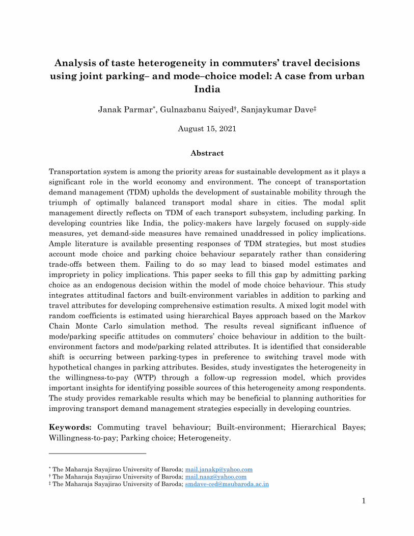
Analysis of taste heterogeneity in commuters’ travel decisions
using joint parking– and mode–choice model: A case from urban
India
Janak Parmar*, Gulnazbanu Saiyed†, Sanjaykumar Dave‡
August 15, 2021
Abstract
Transportation system is among the priority areas for sustainable development as it plays a
significant role in the world economy and environment. The concept of transportation
demand management (TDM) upholds the development of sustainable mobility through the
triumph of optimally balanced transport modal share in cities. The modal split
management directly reflects on TDM of each transport subsystem, including parking. In
developing countries like India, the policy-makers have largely focused on supply-side
measures, yet demand-side measures have remained unaddressed in policy implications.
Ample literature is available presenting responses of TDM strategies, but most studies
account mode choice and parking choice behaviour separately rather than considering
trade-offs between them. Failing to do so may lead to biased model estimates and
impropriety in policy implications. This paper seeks to fill this gap by admitting parking
choice as an endogenous decision within the model of mode choice behaviour. This study
integrates attitudinal factors and built-environment variables in addition to parking and
travel attributes for developing comprehensive estimation results. A mixed logit model with
random coefficients is estimated using hierarchical Bayes approach based on the Markov
Chain Monte Carlo simulation method. The results reveal significant influence of
mode/parking specific attitudes on commuters’ choice behaviour in addition to the built-
environment factors and mode/parking related attributes. It is identified that considerable
shift is occurring between parking-types in preference to switching travel mode with
hypothetical changes in parking attributes. Besides, study investigates the heterogeneity in
the willingness-to-pay (WTP) through a follow-up regression model, which provides
important insights for identifying possible sources of this heterogeneity among respondents.
The study provides remarkable results which may be beneficial to planning authorities for
improving transport demand management strategies especially in developing countries.
Keywords: Commuting travel behaviour; Built-environment; Hierarchical Bayes;
Willingness-to-pay; Parking choice; Heterogeneity.
* The Maharaja Sayajirao University of Baroda; [email protected] † The Maharaja Sayajirao University of Baroda; [email protected] ‡ The Maharaja Sayajirao University of Baroda; [email protected]
2
1. Introduction
The phrase “sustainable development” is one of the most frequently used syntaxes in
current times, and is almost inextricable part of modern politics and economics. This
concept aims at balancing social, economic and technological development that will not
significantly or almost not impact the environment. Transportation system is among
priority areas for sustainable development (Litman, 2017) as it plays significant role in
the world economy and environment. Large metropolitan cities around the world have
been facing ever-increasing automobile population which is frequently cited culprit for
the urban traffic congestion, health and environmental issues, and depletion in
valuable lands. In India, private vehicle stoke has swelled from 45.6 million in 2001 to
182.9 million in 2015 (MoRT&H, India, 2018) and this growth is expected to continue in
future. As per the study by the Boston Consulting Group (2018), leading consequences
like delay and vehicle idling culminate into huge economic loss, estimated as USD 22
billion per year in four major cities Delhi, Kolkata, Mumbai, and Bangalore.
Sustainable transport is one that is accessible, safe, environment-friendly, and
affordable in which congestion, social and economic access are of such levels that they
can be sustained without causing great harm to future generations (ECMT, 2004;
Richardson, 1999). Hence, the concept of transportation demand management (TDM)
upholds the development of sustainable mobility through the triumph of optimally
balanced transport modal share in cities. It directly impacts the TDM of each transport
subsystem, including parking. In developing countries like India, the policy-makers
have largely focused on supply-side measures, such as increasing supply of roads and
promotion of large-scale infrastructure projects like metro-rails, yet demand-side
measures have not been prominently addressed in the policy debate (Chidambaram et
al., 2014). For an efficient design of TDM strategy, it is important to understand
travellers’ needs and decision-making process.
Studying behaviour-pattern of traveller is one of the pivot points in developing policies
that make a travel behaviour more sustainable (Van Wee et al., 2013). This involves
discouraging a travel by private modes and encouraging public transit (PT) and non-
motorized transport (NMT) use. Parking policies are playing an increasingly important
role across the world as a TDM tool in order to achieve these goals. Parking charge is
referred as the second-best alternative to mitigate traffic congestions (Albert and
Mahalel, 2006; Kelly and Clinch, 2006), preceded only by congestion pricing, but it is
more commonly used because it has better acceptance rate among the different user-
groups in comparison with other restrictions (Milosavljevic and Simicevic, 2019,
Chapter 7). Possible reactions to parking policies involve changes in parking type (e.g.,
between on- and off-street parking), parking location, transportation mode, car
occupancy, and frequency and trip-time. Several past studies focused on parking as a
TDM strategy (e.g., Rye et al., 2006; Simićević et al., 2013; Christiansen et al., 2017;
3
Evangolinos et al., 2018), but most studies have considered only an aspect of private
vehicle (PV) use rather than trade-offs between them. Ignoring this realm may lead to
biased model estimates and impropriety in policy implications. For instance, it is likely
that changes in the parking attributes viz. parking cost, search time or walking to
destination elicit parking relocation (e.g., from on-street to off-street parking) instead of
modal shift. In that case, a mode-shift model may decree, for example, parking price
elasticity (with respect to PV choice) to be short of its actual value and subsequently
may lead to wrong interpretations about the efficacy of pricing policy. Besides, parking
strategies may be imposed to relieve parking demand from CBDs by enhancing access
to fringe-parking and to the destination. Beholding to this set-up, it is worth
investigating the parking choice as an endogenous decision within the model of mode
choice behaviour.
This paper seeks to fill this gap by building a joint model of parking and mode choice
and assessing the possible behavioural change that could better address the feasibility
of TDM strategies. In particular, this study develops a joint-model of travel-mode and
parking-choice (on-street & off-street) behaviour for commuters with origin and
destination within the boundary of Delhi-National Capital Region (NCR) in India based
on revealed-preference (RP) data. The model examines the impacts of attitudes toward
parking and travel-modes, parking attributes such as duration, search and walk time,
and built-environment of both work and home locations on commuters’ behaviour. A
mixed logit model with random parameters is estimated using hierarchical Bayes
approach based on the Markov Chain Monte Carlo (MCMC) simulation method. The
study also investigates the taste heterogeneity in the willingness-to-pay (WTP) through
regression model, which provides significant insights to identify possible sources for
this preference heterogeneity among respondents. The results of such an investigation
would enhance the sensitivity of the development strategies and would assist in
accurate formulation of land-use modelling.
The rest of the paper is organized as follows: Section 2 reviews the literature on the
interaction of travel behaviour and above-mentioned measures with additional focus on
parking in brief. Section 3 presents the overview of the methodology, which contains
theoretical framework of the proposed model to estimate the latent variables (section
3.1), choice model based on hierarchical Bayes estimator (section 3.2 and 3.3) and
marginal WTP (section 3.4). Section 4 gives a comprehensive overview of survey as well
as settings and specifications of different variables analysed in the model, followed by
the analysis including measurement model (section 5.1), choice model (section 5.2) and
WTP analysis (section 5.3), and related discussion in Section 5. Lastly, Section 6
discusses the major findings and conclusions drawn from this study.
4
2. Review of Relevant Literature
2.1. Work Trips and Parking
Most of the parking related research has been focused on sensitivity to parking pricing
(Willson and Shoup, 1990; Fearnley and Hanssen, 2012; Nourinejad and Roorda, 2017;
Parmar et al., 2021), role of parking in TDM (Gillen, 1978; Shiftan and Golani, 2005;
Christiansen et al., 2017; Litman 2017), impacts of employer-paid parking (Aldridge et
al., 2006; Su and Zhou, 2012; Pandhe and March, 2012; Brueckner and Franco, 2018). A
common finding of these studies is that the parking pricing policies plays a significant
role in reducing commuter’s private vehicle use. For instance, Willson and Shoup (1990)
analyzed the effects of parking pricing at workplaces in Los Angeles and Washington
D.C. in USA, and Ottawa in Canada based on four before-and-after studies. They
showed 19 to 81 percent reduced car-use by employees if the free parking charges were
eliminated at workplace. Similar kind of study in Norway revealed that commuters
become more positive toward a parking fee led to significant drop in car-use and control
over spillover of parking to local streets (Christiansen, 2014). Su and Zhou (2012)
documented that discounts in parking charges for ride-sharers, reduction in parking
supply or increased parking charges for drive-alone employees are positive steps
employers could take to reduce the share of drive-alone mode of travel. Many
researchers have acknowledged the time-factor as an equally strong metric apart from
parking pricing which influences both travel mode- and parking location-choice
behaviour (e.g., Ibeas et al., 2014; Meng et al., 2017; Yan et al., 2018) buy only a few
travel behaviour studies have incorporated it to analyse its effects. Marsden (2006)
noted that “less evidence is available on observed responses to excess-time, particularly
the time taken between parking vehicle and the final destination of commute trips.” It
may lead to a potential misspecification in mode-choice models and subsequently the
policymakers have vague knowledge about an efficacy of time-factors in TDM and
reducing PV use. Further discussions can be found at Young et al. (1991), Marsden
(2006), Inci (2015) and Parmar et al. (2019).
In addition to reducing PV-use, relieving congestion and parking demand pressure in
CBDs is one of the desirable goals of TDM. A policy based on driver’s parking location
choice has potential to achieve this goal by diminishing cruising for parking (Shoup,
2006) which in turn attracted many studies to analyse driver’s behaviour towards
parking type and location choice (Hunt and Teply, 1993; Hess and Polak, 2004; Ibeas et
al., 2014; Chaniotakis and Pel, 2015; Meng et al., 2017; Hoang et al., 2019). Hess and
Polak (2004) have developed mixed logit (ML) based parking choice model and noticed
significant taste variations in time-factors such as search time for parking space and
walking time to the final destination. Ibeas et al. (2014) did use stated choice data to
model parking choice between on-street and underground parking locations in Santoña,
5
Spain. They assessed the interaction terms defining the effects of the individuals’
characteristics in behaviour. Their study showed parking space search time to be more
important than the time to the final destination. Hoang et al. (2019) compared
multinomial logit (MNL), nested-logit (NL) and mixed-logit (ML) models to evaluate the
parameters influencing motorcycle drivers’ parking location choice behaviour. A
dominated ML model showed that parking pricing, walking to destination, queuing
time (waiting for parking), and capacity of parking lot have significant impacts on
parking choice.
Notwithstanding, most parking studies encompassed the various parking attributes
apart from parking charges, utmost emphasis is given to the consequences of parking
pricing policies at policy level decisions (Except few, e.g., Simićević et al., 2013, Meng et
al., 2017). Additionally, a little amount of research developed conclusions on travel
behaviour (i.e., mode choice) considering the abovementioned parking strategies
(Litman, 2018).
2.2. Travel Behaviour Analysis
Researchers have identified substantial range of variables to evaluate travel behaviour,
typically classified as built environment, mode-specific level-of-service (LOS) attributes,
parking attributes, and subjective attitudes. The effects of parking attributes are
discussed in the previous subsection. This subsection briefly discusses the literature
which incorporated remaining aspects. Knowledge on how built environment shapes the
travel behaviour is one of the critical elements to form sustainable strategies in land-
use planning. Numerous studies have explored the potential of built environment of
both residential and work locations (e.g., Frank et al., 2008; Guan and Wang; 2019) to
control travel behaviour. These factors usually termed as D-factors: density, diversity,
design, distance to transit, and destination accessibility which are well explained by
Ewing and Cervero (2010). Additionally, they found the population and job density have
smaller effects on travel behaviour. However, a few studies indicated strong correlation
between travel behaviour and density (Naess, 2012; Rahul and Verma, 2017). Studies
in developing countries by Zegras and Srinivasn (2006), Sanit et al. (2013) and Rahul
and Verma (2017) found a positive change towards the use of NMT with improved built
environment factors. Studies shown that land-use diversity has significant influence on
travel behaviour. For instance, when residence, work, leisure, and entertainment
locations are adjacent to each other, travel distance will be reduced and subsequently
NMT based trips will be increased and car-trips will be reduced (Cervero and Radisch,
1996; Yue et al., 2016). Besides, the proximity of residence and work-place with respect
to different parts of the city directly affect the urban travel. People living farther from
the city center (e.g., outer fringe of the city) need to travel significantly more by
motorized-mode (Engebretsen and Christiansen, 2011) which reflects the poor
6
accessibility. Also, people working near central parts have lesser car-use and most trips
generally made by NMT or public transit (Rahul and Verma, 2017). Lastly, transit
accessibility also plays critical role in people’s travel behaviour. This may be in terms of
average distance through shortest paths from the residence or workplaces to the
nearest transit station, transit route density within defined area around
origin/destination, distance between transit stops, or the number of stations per unit
area (Ewing and Cervero, 2010).
Apart from the urban form characteristics, psychological characteristics of the
individual traveller, usually known as subjective attitudes have received increased
attention from the researchers in recent years. These studies demonstrated that
individual behaviour pattern is rooted in psychological constructs such as values,
attitudes, subjective norms, perceptions and desires (Abrahamse et al., 2009; Paulssen
et al., 2013). A few studies examined the effects of travel attitudes on car-use and choice
of vehicle type (Steg and Kalfs, 2000; Cao et al., 2009; Van Acker et al., 2014; Etminani-
Ghasrodashti and Ardeshiri, 2015; Guan and Wang, 2019). They showed how the
subjective attitudes along with land-use attributes could influence the travel behaviour.
Paulssen et al. (2013) developed a mixed logit-based model to map the effects of latent
variables (i.e., values and attitudes) on individual’s travel behaviour. Their study
acclaimed that attitudinal factors concerning flexibility, comfort and convenience, and
ownership have greater impacts on travel behaviour than more conventional mode
specific LOS variables. Similarly, Steg and Kalfs (2000) posed that beliefs, preferences
and social norms primarily determine modal choice, much more than by available
alternatives. Therefore, a better understanding of people’s motivations is essential in
order to facilitate shift towards sustainable transport modes from private vehicles.
Generally, modal responses are highly sensitive to the local conditions and
competitiveness of travel modes. For example, in response to parking policy, people may
shift their parking location instead of changing travel mode. As per Marsden (2006),
shift in parking locations is more probable response to parking interventions than
shifting travel mode. Authors are of the opinion that this study is first-of-its-kind in
India which intends to explore the influence of built environment and commuters’
attitudes as well as parking parameters on both parking- and travel mode-choice
behaviour simultaneously.
3. Model Formulation
The model is specified based upon the random utility theory, which assumes that an
individual’s choice would be subjected to the highest utility depending on the
considered parameters as well as unobserved part of this utility. First four subsections
7
describe the mathematical framework followed in this study to develop a model and
analyze WTP, while the remaining subsections explain the data used to fit the model.
3.1. Estimation of Latent Variables
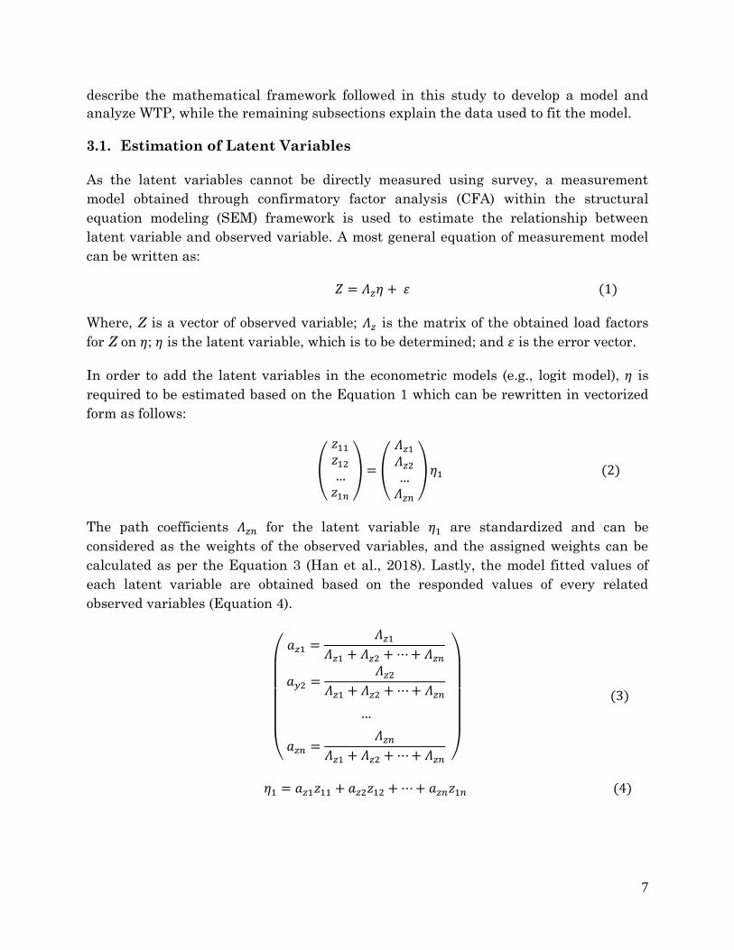
As the latent variables cannot be directly measured using survey, a measurement
model obtained through confirmatory factor analysis (CFA) within the structural
equation modeling (SEM) framework is used to estimate the relationship between
latent variable and observed variable. A most general equation of measurement model
can be written as:
𝑍 = 𝛬𝑧𝜂 + 𝜀 (1)
Where, Z is a vector of observed variable; 𝛬𝑧 is the matrix of the obtained load factors
for Z on 𝜂; 𝜂 is the latent variable, which is to be determined; and 𝜀 is the error vector.
In order to add the latent variables in the econometric models (e.g., logit model), 𝜂 is
required to be estimated based on the Equation 1 which can be rewritten in vectorized
form as follows:
(
𝑧11𝑧12…𝑧1𝑛
) = (
𝛬𝑧1𝛬𝑧2…𝛬𝑧𝑛
) 𝜂1 (2)
The path coefficients 𝛬𝑧𝑛 for the latent variable 𝜂1 are standardized and can be
considered as the weights of the observed variables, and the assigned weights can be
calculated as per the Equation 3 (Han et al., 2018). Lastly, the model fitted values of
each latent variable are obtained based on the responded values of every related
observed variables (Equation 4).
(
𝑎𝑧1 =𝛬𝑧1
𝛬𝑧1 + 𝛬𝑧2 +⋯+ 𝛬𝑧𝑛
𝑎𝑦2 =𝛬𝑧2
𝛬𝑧1 + 𝛬𝑧2 +⋯+ 𝛬𝑧𝑛
…
𝑎𝑧𝑛 =𝛬𝑧𝑛
𝛬𝑧1 + 𝛬𝑧2 +⋯+ 𝛬𝑧𝑛
)
(3)
𝜂1 = 𝑎𝑧1𝑧11 + 𝑎𝑧2𝑧12 +⋯+ 𝑎𝑧𝑛𝑧1𝑛 (4)
8
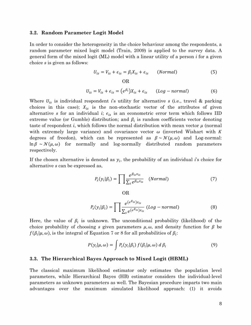
3.2. Random Parameter Logit Model
In order to consider the heterogeneity in the choice behaviour among the respondents, a
random parameter mixed logit model (Train, 2009) is applied to the survey data. A
general form of the mixed logit (ML) model with a linear utility of a person i for a given
choice s is given as follows:
𝑈𝑖𝑠 = 𝑉𝑖𝑠 + 𝜖𝑖𝑠 = 𝛽𝑖𝑋𝑖𝑠 + 𝜖𝑖𝑠 (𝑁𝑜𝑟𝑚𝑎𝑙) (5)
OR
𝑈𝑖𝑠 = 𝑉𝑖𝑠 + 𝜖𝑖𝑠 = (𝑒𝛽𝑖)𝑋𝑖𝑠 + 𝜖𝑖𝑠 (𝐿𝑜𝑔 − 𝑛𝑜𝑟𝑚𝑎𝑙) (6)
Where 𝑈𝑖𝑠 is individual respondent i’s utility for alternative s (i.e., travel & parking
choices in this case); 𝑋𝑖𝑠 is the non-stochastic vector of the attributes of given
alternative s for an individual i; 𝜖𝑖𝑠 is an econometric error term which follows IID
extreme value (or Gumble) distribution; and 𝛽𝑖 is random coefficients vector denoting
taste of respondent i, which follows the normal distribution with mean vector 𝜇 (normal
with extremely large variance) and covariance vector 𝜔 (inverted Wishart with 𝐾
degrees of freedon), which can be represented as 𝛽 ~ 𝒩(𝜇,𝜔) and Log-normal:
ln 𝛽 ~ 𝒩(𝜇, 𝜔) for normally and log-normally distributed random parameters
respectively.
If the chosen alternative is denoted as 𝑦𝑖, the probability of an individual i’s choice for
alternative s can be expressed as,
𝑃𝑠(𝑦𝑖|𝛽𝑖) =∏𝑒𝛽𝑖𝑠𝑥𝑖𝑠
∑ 𝑒𝛽𝑖𝑠𝑥𝑖𝑠𝑠
(𝑁𝑜𝑟𝑚𝑎𝑙) (7)
OR
𝑃𝑠(𝑦𝑖|𝛽𝑖) =∏𝑒(𝑒
𝛽𝑖𝑠)𝑥𝑖𝑠
∑ 𝑒(𝑒𝛽𝑖𝑠)𝑥𝑖𝑠
𝑠
(𝐿𝑜𝑔 − 𝑛𝑜𝑟𝑚𝑎𝑙) (8)
Here, the value of 𝛽𝑖 is unknown. The unconditional probability (likelihood) of the
choice probability of choosing s given parameters 𝜇,𝜔, and density function for 𝛽 be
𝑓(𝛽𝑖|𝜇, 𝜔), is the integral of Equation 7 or 8 for all probabilities of 𝛽𝑖:
𝑃(𝑦𝑖|𝜇, 𝜔) = ∫𝑃𝑠(𝑦𝑖|𝛽𝑖) 𝑓(𝛽𝑖|𝜇, 𝜔) 𝑑 𝛽𝑖 (9)
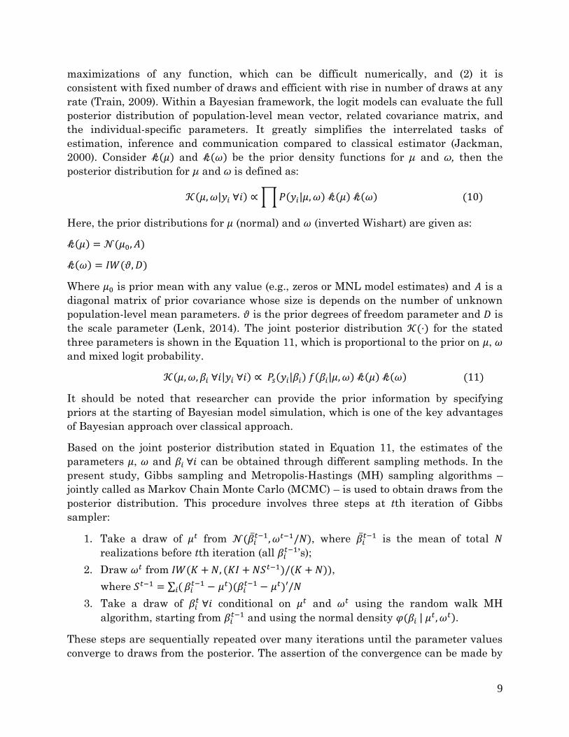
3.3. The Hierarchical Bayes Approach to Mixed Logit (HBML)
The classical maximum likelihood estimator only estimates the population level
parameters, while Hierarchical Bayes (HB) estimator considers the individual-level
parameters as unknown parameters as well. The Bayesian procedure imparts two main
advantages over the maximum simulated likelihood approach: (1) it avoids
9
maximizations of any function, which can be difficult numerically, and (2) it is
consistent with fixed number of draws and efficient with rise in number of draws at any
rate (Train, 2009). Within a Bayesian framework, the logit models can evaluate the full
posterior distribution of population-level mean vector, related covariance matrix, and
the individual-specific parameters. It greatly simplifies the interrelated tasks of
estimation, inference and communication compared to classical estimator (Jackman,
2000). Consider 𝓀(𝜇) and 𝓀(𝜔) be the prior density functions for μ and ω, then the
posterior distribution for μ and ω is defined as:
𝒦(𝜇, 𝜔|𝑦𝑖 ∀𝑖) ∝∏𝑃(𝑦𝑖|𝜇, 𝜔) 𝓀(𝜇) 𝓀(𝜔) (10)
Here, the prior distributions for 𝜇 (normal) and 𝜔 (inverted Wishart) are given as:
𝓀(𝜇) = 𝒩(𝜇0, 𝐴)
𝓀(𝜔) = 𝐼𝑊(𝜗, 𝐷)
Where 𝜇0 is prior mean with any value (e.g., zeros or MNL model estimates) and 𝐴 is a
diagonal matrix of prior covariance whose size is depends on the number of unknown
population-level mean parameters. 𝜗 is the prior degrees of freedom parameter and 𝐷 is
the scale parameter (Lenk, 2014). The joint posterior distribution 𝒦(·) for the stated
three parameters is shown in the Equation 11, which is proportional to the prior on 𝜇, 𝜔
and mixed logit probability.
𝒦(𝜇,𝜔, 𝛽𝑖 ∀𝑖|𝑦𝑖 ∀𝑖) ∝ 𝑃𝑠(𝑦𝑖|𝛽𝑖) 𝑓(𝛽𝑖|𝜇, 𝜔) 𝓀(𝜇) 𝓀(𝜔) (11)
It should be noted that researcher can provide the prior information by specifying
priors at the starting of Bayesian model simulation, which is one of the key advantages
of Bayesian approach over classical approach.
Based on the joint posterior distribution stated in Equation 11, the estimates of the
parameters 𝜇, 𝜔 and 𝛽𝑖 ∀𝑖 can be obtained through different sampling methods. In the
present study, Gibbs sampling and Metropolis-Hastings (MH) sampling algorithms –
jointly called as Markov Chain Monte Carlo (MCMC) – is used to obtain draws from the
posterior distribution. This procedure involves three steps at tth iteration of Gibbs
sampler:
1. Take a draw of 𝜇𝑡 from 𝒩(�̅�𝑖𝑡−1, 𝜔𝑡−1/𝑁), where �̅�𝑖
𝑡−1 is the mean of total 𝑁
realizations before tth iteration (all 𝛽𝑖𝑡−1’s);
2. Draw 𝜔𝑡 from 𝐼𝑊(𝐾 +𝑁, (𝐾𝐼 + 𝑁𝑆𝑡−1)/(𝐾 + 𝑁)),
where 𝑆𝑡−1 = ∑ (𝑖 𝛽𝑖𝑡−1 − 𝜇𝑡)(𝛽𝑖
𝑡−1 − 𝜇𝑡)′/𝑁
3. Take a draw of 𝛽𝑖𝑡 ∀𝑖 conditional on 𝜇𝑡 and 𝜔𝑡 using the random walk MH
algorithm, starting from 𝛽𝑖𝑡−1 and using the normal density 𝜑(𝛽𝑖 | 𝜇
𝑡, 𝜔𝑡).
These steps are sequentially repeated over many iterations until the parameter values
converge to draws from the posterior. The assertion of the convergence can be made by
10
examining if the draws after burn-in period are moving around the posterior (Train,
2009).
3.4. Estimation of Marginal Willingness-to-pay (MWTP)
The proposed model allows random coefficients to capture the taste heterogeneity in
choice behaviour. Considering the distribution of 𝛽𝑖 for a given sampled population be
𝑓(𝛽𝑖|𝜇, 𝜔) and joint posterior for 𝜇, 𝜔 and 𝛽𝑖 ∀𝑖 as defined in Equation 11, the
conditional probability (posterior) of respondent’s choice can be defined as:
𝐻𝑖𝑠(𝛽𝑖|𝜇, 𝜔, 𝑦𝑖 ∀𝑖) =𝑃𝑠(𝑦𝑖|𝛽𝑖) 𝑓(𝛽𝑖|𝜇, 𝜔)
∫𝑃𝑠(𝑦𝑖|𝛽𝑖) 𝑓(𝛽𝑖|𝜇, 𝜔) 𝑑 𝛽𝑖 (12)
Since, the quantities on the RHS of Equation 12 is known as a result of the choice
model, the mean 𝛽𝑖 for each respondent 𝑖 in the sampled population for choosing 𝑦𝑖 can
be obtained as:
𝛽𝑖= 𝐸(𝛽𝑖|𝜇, 𝜔, 𝑦𝑖 ∀𝑖) = ∫𝛽𝑖𝐻𝑖𝑠(𝛽𝑖|𝜇, 𝜔, 𝑦𝑖 ∀𝑖) 𝑑 𝛽𝑖
=∬…∫𝛽𝑖𝒦(𝜇, 𝜔, 𝛽𝑖 ∀𝑖|𝑦𝑖 ∀𝑖) 𝑑𝜇 𝑑𝜔 𝑑𝛽1 𝑑𝛽2… 𝑑𝛽𝐼 (13)
The above multidimensional integral does not have a closed form, and is approximated
through simulation. In HB model, the draws for 𝜇, 𝜔 and 𝛽𝑖 ∀𝑖 are obtained from their
joint posterior defined in Equation 11. If 𝛽𝑖𝑎
be the coefficient of attribute 𝑎 for
individual 𝑖 and 𝛽𝑐 be the cost coefficient, then the individual-specific MWTP can be
calculated as:
𝑀𝑊𝑇𝑃𝑖𝑎 = −𝛽𝑖𝑎
𝛽𝑐 (14)
Once the individual level MWTP is estimated, the variations in calculated MWTP
among the individuals can be analysed by establishing the relationship between
possible sources (e.g., socioeconomic characteristics) and MWTP through regression.
This type of two-step approach was used in a very few studies in different aspects
(Campbell, 2007; Hoshino, 2011) to analyse the preference heterogeneity in choice
behaviour, but yet to be explored in the context of travel behaviour. These studies
showed that this approach yielded greater validity and explanatory power than
standard methods used to incorporate individual-specific variables into the analysis.
The MWTP regression in this study assumes that respondents’ socioeconomic
characteristics primarily influence the heterogeneity in MWTP. Based on the individual
MWTP calculated using Equation 14, and considering 𝑞𝑖𝑎 be a vector of respondent 𝑖’s
socioeconomic characteristics, the regression model can be expressed as:
𝑀𝑊𝑇𝑃𝑖𝑎 = 𝛼𝑎 + 𝛾𝑎′ 𝑞𝑖𝑎 + 𝜀𝑖𝑎 (15)
11
Where, 𝛼𝑎 is an intercept, which is constant for all individuals; 𝛾𝑎′ is the coefficient
vector; and 𝜀𝑖𝑎 is an unobserved random term reflecting the effect of omitted variables.
4. Survey and Data Description
For this study, data were collected through face-to-face interview survey of commuters
(students were not included) in Delhi, India. The urban population of the city was
estimated as 26 million (97.5% share), making it the world’s second largest urban areas
and comprises second-highest GDP per capita in India (Planning Dept., 2019). The city
has been experiencing perturbing inflation in traffic congestion and air pollution in past
two decades which are the consequences of the rapidly soared motor-vehicle population.
Currently, it has 11.27 million of registered vehicles in terms of cars, jeeps and
motorized two-wheelers (MTW) sharing nearly 95% of the total vehicles (Economic
Survey of Delhi, 2021). Additionally, they demand huge space for parking in CBD areas
to waste valuable land resources. It is estimated that the annual demand for car
parking space in Delhi can be equivalent to as much as 471 football fields. Public
transit in Delhi has two major services- bus (fleet size of 6572) and metro, having daily
ridership of nearly 11 million as per Economic Survey of Delhi (2021). The public
transit share is near to 50%, while private vehicles including cars and MTW cater to
about 32% of total motorized trips in the city.
This study used the data collected through RP survey conducted between September to
November 2019 in Delhi. Respondents were recruited randomly at their work locations
in order to complete the survey form making sure that the respondent is eligible for the
interview (i.e., the trip is within study area, had an alternative transport mode and
parking-type available to use). A questionnaire includes the information regarding
personal and household (HH) characteristics, vehicle-ownership levels, trip and parking
related attributes, and access/egress details. It also comprises several modes- and
parking-specific attitudinal statements on a 5-point Likert-scale from “strongly
disagree” to “strongly agree”. The collected data was continuously monitored while
survey was in progress to ensure a good balance of data spreading across the city and
having well distributed trip characteristics. A total of 650 respondents were
interviewed of which 602 samples were refined (excluding unqualified and incorrect
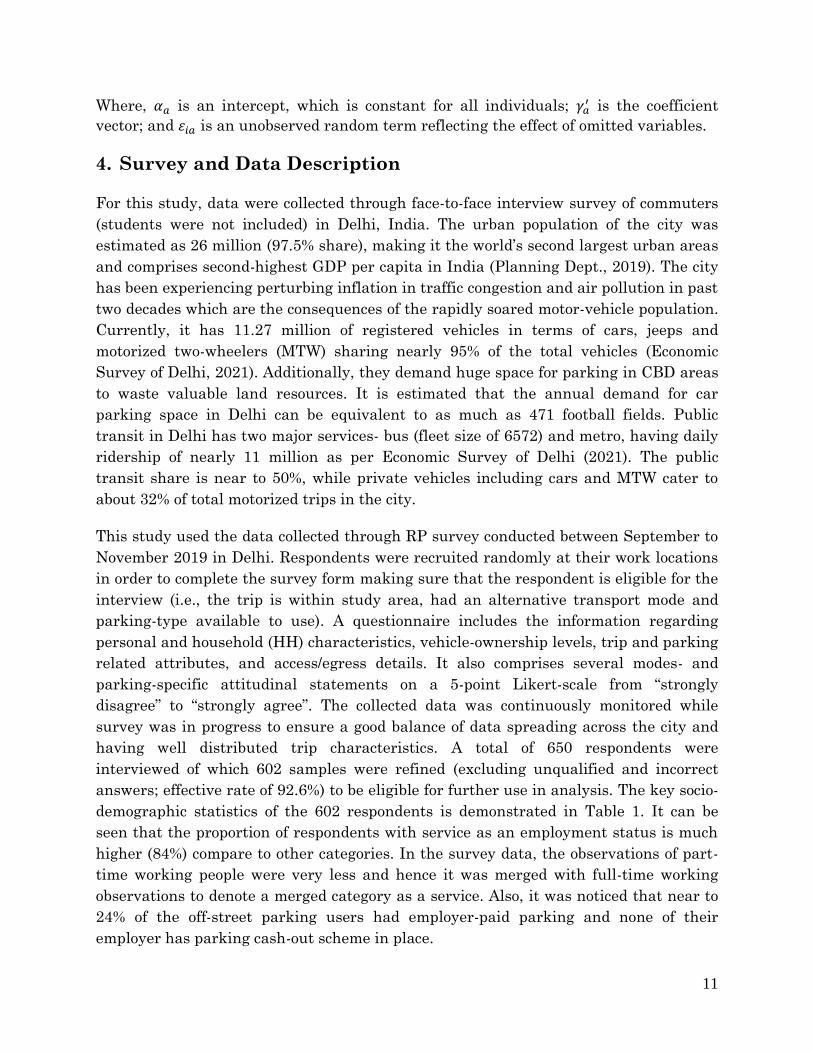
answers; effective rate of 92.6%) to be eligible for further use in analysis. The key socio-
demographic statistics of the 602 respondents is demonstrated in Table 1. It can be
seen that the proportion of respondents with service as an employment status is much
higher (84%) compare to other categories. In the survey data, the observations of part-
time working people were very less and hence it was merged with full-time working
observations to denote a merged category as a service. Also, it was noticed that near to
24% of the off-street parking users had employer-paid parking and none of their
employer has parking cash-out scheme in place.
12
Table 1 Descriptive Statistics of analysed samples
Individual Characteristics Category Frequency (%)
Sex Male 404 (67.1)
Female 198 (32.9)
Age 18 – 24 13 (2.2)
25 – 39 351 (58.3)
40 – 64 238 (39.5)
Income
(Thousand ₹)
< 20 66 (11)
20 – 35 204 (33.9)
35 – 50 129 (21.4)
50 – 70 76 (12.6)
> 70 127 (21.1)
Education level Primary-school 4 (0.7)
High-school 122 (20.3)
Graduate 393 (65.3)
Postgraduate and higher 83 (13.8)
Employment Status Service 506 (84)
Business 36 (6)
Self-employed 60 (10)
Current Transport Mode* Car & Off-street parking
(Car_Off)
104 (17.3) [37.55]
Car & On-street parking
(Car_On)
46 (7.6) [16.61]
Motorcycle & Off-street parking
(MTW_Off)
68 (11.3) [14.08]
Motorcycle & On-street parking
(MTW_On)
84 (13.9) [17.39]
Public transport– Bus 148 (24.6) [24.58]
Public transport– Metro 100 (16.6) [16.61]
Non-motorized modes (NMT) 52 (8.6) [42.28]
Household Characteristics Mean (Std. Dev.)
Members in HH 3.83 (1.44)
Number of working members 1.65 (0.65)
Number of Cars in HH 0.53 (0.63)
Number of MTW in HH 1.06 (0.68)
Number of Bicycles in HH 0.69 (0.61)
* The values in square brackets show percent times chosen when available/feasible.
13
The trip features such as trip distance, trip time (purely an in-vehicle time), trip cost,
and parking features such as parking duration, search time for parking space, and walk
time to destination (i.e., egress time) were considered in this study. All these indicators
were self-reported by the respondents. The average travel distance across all modes
was observed to be about 10 km which is also an average commute distance across the
Delhi-NCR. For trip time, only in-vehicle time was considered as a trip attribute. This
is because the access and egress features for public modes are taken as BE factors
whereas for the private modes, access features are neglected as people park their
vehicles right in-front of their homes and egress features are considered within parking
attributes. Trip cost is estimated on monthly-basis in this study because for PV
categories, maintenance cost is also taken into account in addition to fuel cost to
demonstrate the full cost people incur for using PVs. In a similar fashion, monthly
charges for using PT (either daily tickets or monthly pass) were asked to the
respondents in the survey. To distinguish between the on-street and off-street parking,
parking demand in terms of duration, search time for parking space, and egress time
for both the parking types were considered. Though the parking price is one of the most
important deciding factors in parking choice, it was not taken into account, because as
per the current scenario, the parking price for both on-street and off-street parking is
same in study location. Further, the current parking tariff is ₹20 per hour with the
maximum of ₹100 per day for car, and ₹10 per hour with the maximum of ₹50 per day
for MTW in the city. Since the minimum parking duration is greater than 5 hours as
per the data, parking cost incur to PV users become constant to all individuals. In this
sense, it does not have influence on commuters’ parking choice decision.
4.1. Built Environment Factors
Using the information developed from the geo-coded land use database, several spatial
characteristics of the built environment were estimated in this study. A political ward
map (272 wards) was considered as a base map to identify the origin and destination of
the respondents on the map. The built environment factors include land use diversity
(entropy index), road density, working population density, and accessibility– distance
from home and work location to the closest metro station and closest bus stop (self-
reported). It should be noted that density and diversity indicators are calculated at the
trip origins only.
4.2. Attitudinal Factors
As this study tries to identify objective as well as subjective influences on commute
travel behaviour, individuals’ attitudinal preferences towards travel modes and parking
were captured in the survey. The list of the statements regarding attitudes included in
the survey is shown in the Appendix. The responses to these statements were then
14
factor analysed using principal axis factoring method (promax rotation) to find out how
they can be related to each other. The factors (latent variables) were extracted from
these observed attitudes for individual modes to understand which latent variables are
important to which specific mode. Cronbach’s alpha was used to measure the internal
consistency i.e., how closely a set of indicators for each latent variable related to each
other in a same group. The obtained alpha values for each group were acceptable (∝ >
0.7) as listed in the respective Tables in Appendix. Additionally, Pearson’s correlation
matrix presented high correlation values between factors which also support the factor
analysis used in this study. The Kaiser-Meyer-Olkin’s (KMO) sampling adequacy test
was employed to check the suitability of data for factor analysis. The latent variables
obtained from the observed attitudes are: 1. Individualist, pro-environment, economy,
comfort, and flexibility for PVs (68.63% variance explained, KMO = 0.73); 2. Comfort,
convenience, safety, and flexibility for PT (60.76% variance explained, KMO = 0.69); 3.
Health, safety, comfort, and convenience for NMT modes (71.78% variance explained,
KMO = 0.81); and Safety and convenience for Parking types (59.85% variance
explained, KMO = 0.71). Next, confirmatory factor analysis (CFA) was conducted within
the structural equation modeling (SEM) framework to validate the relationships
between the observed and latent variables, which is discussed in the next section.
5. Model Estimation and Results
5.1. The Measurement Model
After ensuring the adequacy of the factor analysis, CFA models (also known as
measurement model) were developed for each transport modes group (i.e., PV, PT &
NMT) and parking type in order to obtain the path coefficients. As the observed
attitudes were considered as ordered-categorical variables, diagonally weighted least
squares (DWLS) estimator with the bounds constrained quasi-Newton optimizer was
used to estimate path coefficients. This approach uses the WLS estimator with
polychoric correlations as input to create an asymptotic covariance matrix. In this
model, the ordered categories are considered as discretized normally distributed latent
continuous response through a number of threshold parameters (see, Muthén, 1994).
These thresholds denote values of the latent continuous variable where respondents
cross over from one ordinal category to the next. The method is typically paired with
robust estimation adjustments (called “sandwich” estimator) that improves chi-square,
standard error, and fit indices and observed to perform statistically better as well
(Rhemtulla et al., 2012).
The estimated path coefficients for each indicator subjected to the respective latent
variable are presented in the Tables 2, 3, 4 and 5. It can be seen that all the estimated
coefficients had the expected sign and significant at the 90% confidence level or higher.
15
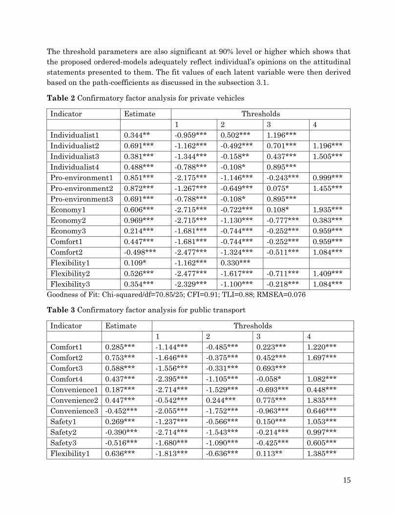
The threshold parameters are also significant at 90% level or higher which shows that
the proposed ordered-models adequately reflect individual’s opinions on the attitudinal
statements presented to them. The fit values of each latent variable were then derived
based on the path-coefficients as discussed in the subsection 3.1.
Table 2 Confirmatory factor analysis for private vehicles
Indicator Estimate Thresholds
1 2 3 4
Individualist1 0.344** -0.959*** 0.502*** 1.196***
Individualist2 0.691*** -1.162*** -0.492*** 0.701*** 1.196***
Individualist3 0.381*** -1.344*** -0.158** 0.437*** 1.505***
Individualist4 0.488*** -0.788*** -0.108* 0.895***
Pro-environment1 0.851*** -2.175*** -1.146*** -0.243*** 0.999***
Pro-environment2 0.872*** -1.267*** -0.649*** 0.075* 1.455***
Pro-environment3 0.691*** -0.788*** -0.108* 0.895***
Economy1 0.606*** -2.715*** -0.722*** 0.108* 1.935***
Economy2 0.969*** -2.715*** -1.130*** -0.777*** 0.383***
Economy3 0.214*** -1.681*** -0.744*** -0.252*** 0.959***
Comfort1 0.447*** -1.681*** -0.744*** -0.252*** 0.959***
Comfort2 -0.498*** -2.477*** -1.324*** -0.511*** 1.084***
Flexibility1 0.109* -1.162*** 0.330***
Flexibility2 0.526*** -2.477*** -1.617*** -0.711*** 1.409***
Flexibility3 0.354*** -2.329*** -1.100*** -0.218*** 1.084***
Goodness of Fit: Chi-squared/df=70.85/25; CFI=0.91; TLI=0.88; RMSEA=0.076
Table 3 Confirmatory factor analysis for public transport
Indicator Estimate Thresholds
1 2 3 4
Comfort1 0.285*** -1.144*** -0.485*** 0.223*** 1.220***
Comfort2 0.753*** -1.646*** -0.375*** 0.452*** 1.697***
Comfort3 0.588*** -1.556*** -0.331*** 0.693***
Comfort4 0.437*** -2.395*** -1.105*** -0.058* 1.082***
Convenience1 0.187*** -2.714*** -1.529*** -0.693*** 0.448***
Convenience2 0.447*** -0.542*** 0.244*** 0.775*** 1.835***
Convenience3 -0.452*** -2.055*** -1.752*** -0.963*** 0.646***
Safety1 0.269*** -1.237*** -0.566*** 0.150*** 1.053***
Safety2 -0.390*** -2.714*** -1.543*** -0.214*** 0.997***
Safety3 -0.516*** -1.680*** -1.090*** -0.425*** 0.605***
Flexibility1 0.636*** -1.813*** -0.636*** 0.113** 1.385***
16
Flexibility2 0.623*** -0.868*** 0.054* 0.527*** 1.332***
Flexibility3 0.546*** -2.022*** -0.736*** 0.142*** 1.529***
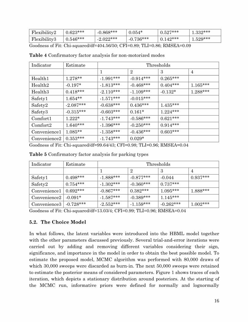
Goodness of Fit: Chi-squared/df=404.56/50; CFI=0.89; TLI=0.86; RMSEA=0.09
Table 4 Confirmatory factor analysis for non-motorized modes
Indicator Estimate Thresholds
1 2 3 4
Health1 1.278** -1.991*** -0.914*** 0.265***
Health2 -0.197* -1.813*** -0.468*** 0.404*** 1.165***
Health3 0.418*** -2.110*** -1.109*** -0.132* 1.288***
Safety1 1.654** -1.571*** -0.015***
Safety2 -2.087*** -0.638*** 0.436*** 1.435***
Safety3 -0.315*** -0.603*** 0.161* 1.224***
Comfort1 1.222* -1.743*** -0.586*** 0.621***
Comfort2 1.640*** -1.396*** -0.250*** 0.914***
Convenience1 1.085** -1.358*** -0.436*** 0.603***
Convenience2 0.353*** -1.743*** 0.029*
Goodness of Fit: Chi-squared/df=99.64/43; CFI=0.98; TLI=0.96; RMSEA=0.04
Table 5 Confirmatory factor analysis for parking types
Indicator Estimate Thresholds
1 2 3 4
Safety1 0.498*** -1.888*** -0.877*** -0.044 0.937***
Safety2 0.754*** -1.302*** -0.360*** 0.737***
Convenience1 0.692*** -0.867*** 0.382*** 1.095*** 1.888***
Convenience2 -0.091* -1.587*** -0.389*** 1.145***
Convenience3 -0.728*** -2.552*** -1.159*** -0.262*** 1.002***
Goodness of Fit: Chi-squared/df=13.03/4; CFI=0.99; TLI=0.96; RMSEA=0.04
5.2. The Choice Model
In what follows, the latent variables were introduced into the HBML model together
with the other parameters discussed previously. Several trial-and-error iterations were
carried out by adding and removing different variables considering their sign,
significance, and importance in the model in order to obtain the best possible model. To
estimate the proposed model, MCMC algorithm was performed with 80,000 draws of
which 30,000 sweeps were discarded as burn-in. The next 50,000 sweeps were retained
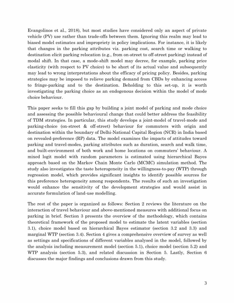
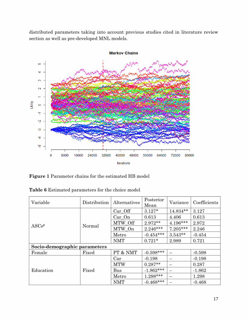
to estimate the posterior means of considered parameters. Figure 1 shows traces of each
iteration, which depicts a stationary distribution around posteriors. At the starting of
the MCMC run, informative priors were defined for normally and lognormally
17
distributed parameters taking into account previous studies cited in literature review
section as well as pre-developed MNL models.
Figure 1 Parameter chains for the estimated HB model
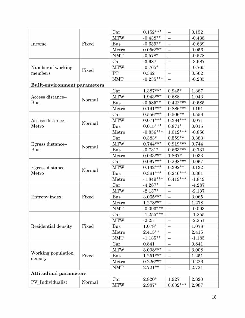
Table 6 Estimated parameters for the choice model
Variable Distribution Alternatives Posterior
Mean Variance Coefficients
ASCs# Normal
Car_Off 3.127* 14.834** 3.127
Car_On 0.613 4.406 0.613
MTW_Off 2.972** 4.196*** 2.972
MTW_On 2.246*** 7.205*** 2.246
Metro -0.454*** 3.543** -0.454
NMT 0.721* 2.989 0.721
Socio-demographic parameters
Female Fixed PT & NMT -0.598*** – -0.598
Education Fixed
Car -0.198 – -0.198
MTW 0.287** – 0.287
Bus -1.862*** – -1.862
Metro 1.298*** – 1.298
NMT -0.468*** – -0.468
18
Income Fixed
Car 0.152*** – 0.152
MTW -0.438** – -0.438
Bus -0.639** – -0.639
Metro 0.056*** – 0.056
NMT -0.578* – -0.578
Number of working
members Fixed
Car -3.687 – -3.687
MTW -0.765* – -0.765
PT 0.562 – 0.562
NMT -0.235*** – -0.235
Built-environment parameters
Access distance–
Bus Normal
Car 1.387*** 0.945* 1.387
MTW 1.943*** 0.688 1.943
Bus -0.585** 0.422*** -0.585
Metro 0.191*** 0.886*** 0.191
Access distance–
Metro Normal
Car 0.556*** 0.506** 0.556
MTW 0.071*** 0.384*** 0.071
Bus 0.015*** 0.871* 0.015
Metro -0.856*** 1.012*** -0.856
Egress distance–
Bus Normal
Car 0.383* 0.559** 0.383
MTW 0.744*** 0.919*** 0.744
Bus -0.731* 0.663*** -0.731
Metro 0.033*** 1.867* 0.033
Egress distance–
Metro Normal
Car 0.067*** 0.298*** 0.067
MTW 0.132*** 0.392** 0.132
Bus 0.361*** 0.246*** 0.361
Metro -1.849*** 0.419*** -1.849
Entropy index Fixed
Car -4.287* – -4.287
MTW -2.137* – -2.137
Bus 3.065*** – 3.065
Metro 1.278*** – 1.278
NMT -0.093*** – -0.093
Residential density Fixed
Car -1.255*** – -1.255
MTW -2.251 – -2.251
Bus 1.078* – 1.078
Metro 2.415** – 2.415
NMT -1.185** – -1.185
Working population
density Fixed
Car 0.841 – 0.841
MTW 3.008*** – 3.008
Bus 1.251*** – 1.251
Metro 0.226*** – 0.226
NMT 2.721** – 2.721
Attitudinal parameters
PV_Individualist Normal Car 2.820* 1.927 2.820
MTW 2.987* 0.632*** 2.987
19
PV_Pro-environment Normal Car -1.120*** 3.993*** -1.120
MTW -0.624*** 1.819** -0.624
PV_Economy Normal Car -2.515*** 0.393 -2.515
MTW 0.739*** 1.116*** 0.739
PV_Comfort Normal Car 1.882*** 0.941* 1.882
MTW 3.120 1.112* 3.12
PV_Flexibility Normal Car -0.953*** 2.108*** -0.953
Parking_Safety Normal
Car_Off 2.519** 0.785* 2.519
Car_On -1.662*** 0.392** -1.662
MTW_Off 1.020*** 0.981*** 1.020
MTW_On -0.071* 0.106** -0.071
Parking_Convenience Normal
Car_Off -1.054** 0.835* -1.054
Car_On 0.953*** 0.877** 0.953
MTW_Off -1.691*** 1.084* -1.691
MTW_On 2.073* 1.238*** 2.073
PT_Comfort Normal
Car 1.695 1.077*** 1.695
MTW 2.703*** 1.793* 2.703
Bus 2.156** 2.594 2.156
Metro -0.906 3.151* -0.906
NMT -0.452** 3.613** -0.452
PT_Convenience Normal
Car 0.517 2.983* 0.517
MTW 0.978*** 2.129*** 0.978
Bus -1.502*** 0.804*** -1.502
Metro 1.851 0.763** 1.851
NMT -1.062*** 0.536*** -1.062
PT_Safety Normal Bus -2.636*** 0.832* -2.636
Metro -1.426** 1.117*** -1.426
PT_Flexibility Normal
Car -0.368 2.030** -0.368
MTW 0.799** 4.700*** 0.799
Bus 0.927 1.205 0.927
Metro 0.829 0.654* 0.829
NMT -0.615 7.239 -0.615
NMT_Health Normal
Car -0.658** 0.763*** -0.658
MTW -0.632** 1.926** -0.632
Bus -1.82 1.858 -1.82
NMT 4.320** 1.661*** 4.320
NMT_Safety Normal
Car 1.355*** 4.849*** -1.355
MTW 0.084** 0.962*** -0.084
Bus 0.866*** 0.612** -0.866
NMT -2.278** 1.207* -2.278
NMT_Comfort Normal
Car 0.457*** 0.980** 0.457
MTW 1.045* 2.992*** 1.045
Bus -1.201*** 1.110* -1.201
NMT -1.467*** 0.257 -1.467
20
NMT_Convenience Normal
Car -0.719*** 0.395* -0.719
MTW 0.070*** 0.791 0.070
Bus 0.048*** 1.15 0.048
NMT 1.745* 1.772** 1.745
Parking & travel parameters
Employer paid
parking Fixed
Car_Off 1.075*** – 1.075
MTW_Off 1.902** – 1.902
PT -0.883 – -0.883
Parking duration Normal
Car_Off 2.152* 0.448** 2.152
Car_On -0.863* 0.296* -0.863
MTW_Off 1.852** 0.885* 1.852
MTW_On -0.558*** 0.331** -0.558
Parking search time Lognormal
Car_Off -0.122*** 0.525*** -1.151
Car_On -0.035*** 0.227** -1.082
MTW_Off -0.024 1.443* -2.009
MTW_On -0.028*** 0.447* -1.216
Parking egress time Lognormal
Car_Off -0.041* 0.323*** -1.128
Car_On -0.050*** 0.723** -1.366
MTW_Off -0.025*** 0.572** -1.298
MTW_On -0.099*** 0.509*** -1.168
In-vehicle travel time Lognormal
Car -0.115*** 1.006** -1.477
MTW -0.076* 0.858 -1.424
Bus -0.181** 2.069*** -2.377
Metro -0.119* 0.364* -1.064
NMT -0.131* 0.420*** -1.083
Trip cost (₹) Lognormal
Car -0.033*** 0.294*** -1.121
MTW -0.052*** 1.271** -1.792
Bus -0.058*** 0.652* -1.307
Metro -0.061*** 0.279*** -1.081
Trip distance (km) Fixed
Car 0.669* – 0.669
MTW -0.489* – -0.489
Bus 0.399** – 0.399
Metro 1.382* – 1.382
NMT -1.547*** – -1.547
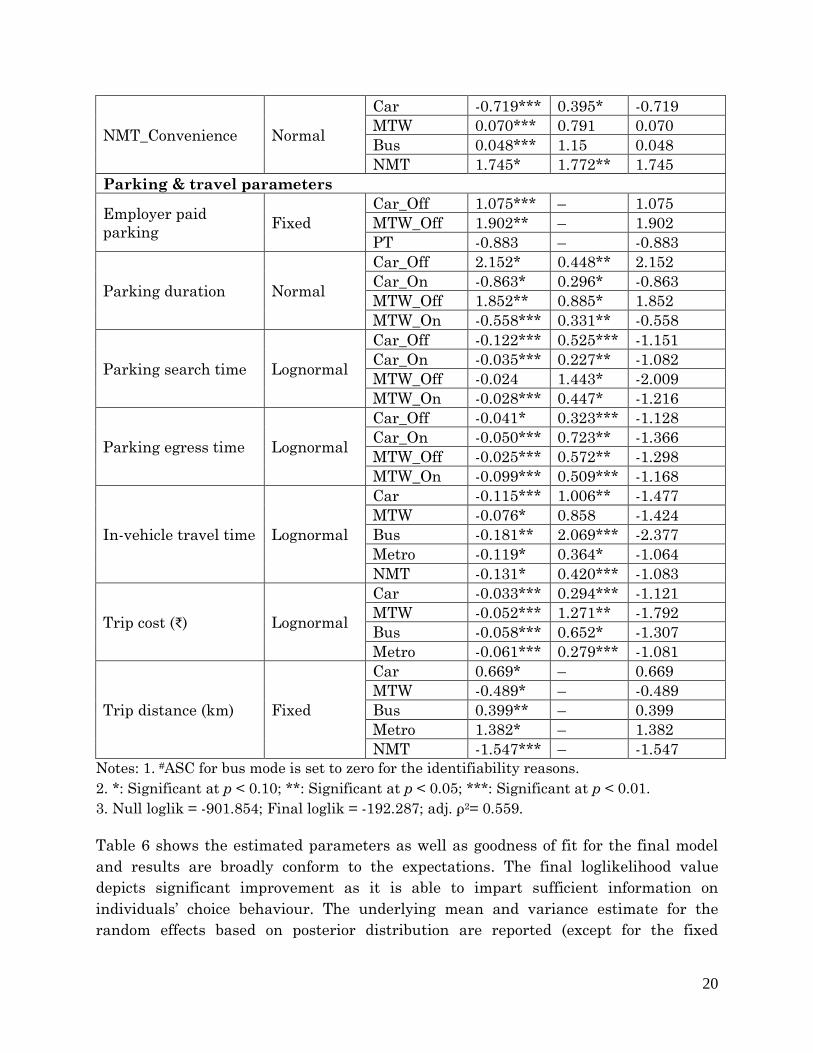
Notes: 1. #ASC for bus mode is set to zero for the identifiability reasons.
2. *: Significant at p < 0.10; **: Significant at p < 0.05; ***: Significant at p < 0.01.
3. Null loglik = -901.854; Final loglik = -192.287; adj. ρ2= 0.559.
Table 6 shows the estimated parameters as well as goodness of fit for the final model
and results are broadly conform to the expectations. The final loglikelihood value
depicts significant improvement as it is able to impart sufficient information on
individuals’ choice behaviour. The underlying mean and variance estimate for the
random effects based on posterior distribution are reported (except for the fixed
21
parameters). Most of the parameters are significant at 90% or higher confidence level.
A significant heterogeneity in more or less amount is observed for all parameters, as
evidenced by the significant variances, which the standard logit model is unable to
capture. A few non-significant parameters were also retained in model as they provide
important information regarding respondents’ decision-making.
The ASCs in the model show that all the modes but metro was preferable over bus
given the availability. Further, the magnitude is observed to be higher for private
modes (car & MTW) compare to others. It is noticed that the utility of the private modes
increases with the increased income, also the use of metro is observed to increase but
the coefficient is less in magnitude. These results are in line with the higher mode
share for private transport observed in New Delhi. The probability of increased modal
share of public transport modes improves as the number of working members rises in a
family. The primary reasons for this might be the limited vehicle ownership and
different work places for the family members.
The built-environment factors also exhibit significant influence especially on the mode-
choice which are in line with the past studies discussed in LITERATURE. In the model,
access distance for metro was not found significant and hence removed. It is seen that
the propensity to ride with bus decreases with increase in access distance as the
coefficient of bus possessed negative sign for access distance. In a similar fashion, the
coefficients of egress distance to both bus and metro are negative for the respective
modes. That is, when egress distance increases, the probability of using bus and metro
for commuting decreases. It can be noticed that the coefficient of egress distance from
bus stop is comparatively much lesser, which means the tendency to shift from bus
mode is not very high. The entropy index has a negative effect on car, MTW, and NMT
modes, while it is positive for the bus and metro. It reveals that the more diversified the
land-use, the higher will be use of public modes of transport. Unlike previous works,
this model shows that use of NMT decreases for higher entropy index, though the
magnitude of the coefficient is much lower. The model results for residential density
demonstrate that the use of public transport modes is positively related to the denser
urban area. Further, it can be perceived that people are likely to use MTW or bus for
travel or to walk to a greater extent when they reside in the area with higher working
population density.
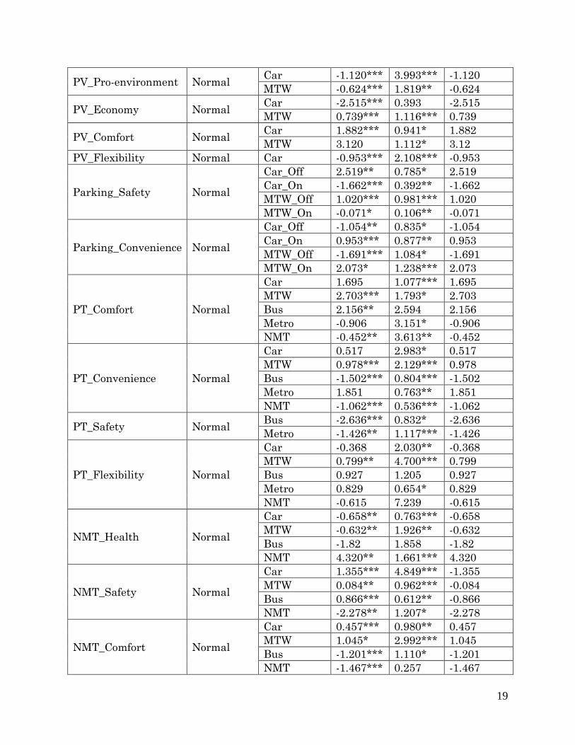
Looking to the model, almost all considered attitudinal factors are significantly related
to mode-choice behaviour, indicating that these attitudinal parameters are
determinants for mode choice. PV_Individualist attitude has a significant positive
impact on private mode use for commuters. The proposed model allows to calculate the
probability given the coefficient for an attribute as the density function for the
coefficient vector 𝛽𝑖, 𝒩(𝜇,𝜔) is now known. Hence, the probability given the positive
coefficient for PV_Individualist for car can be estimated as P(𝛽𝑃𝑉_𝐼𝑛𝑑𝑖𝑣𝑖𝑑𝑢𝑎𝑙𝑖𝑠𝑡 > 0) = 0.979,
which suggests that almost all respondents prefer to use car when their attitude is
positively associated with the related response to the statements. Similar is the case for
22
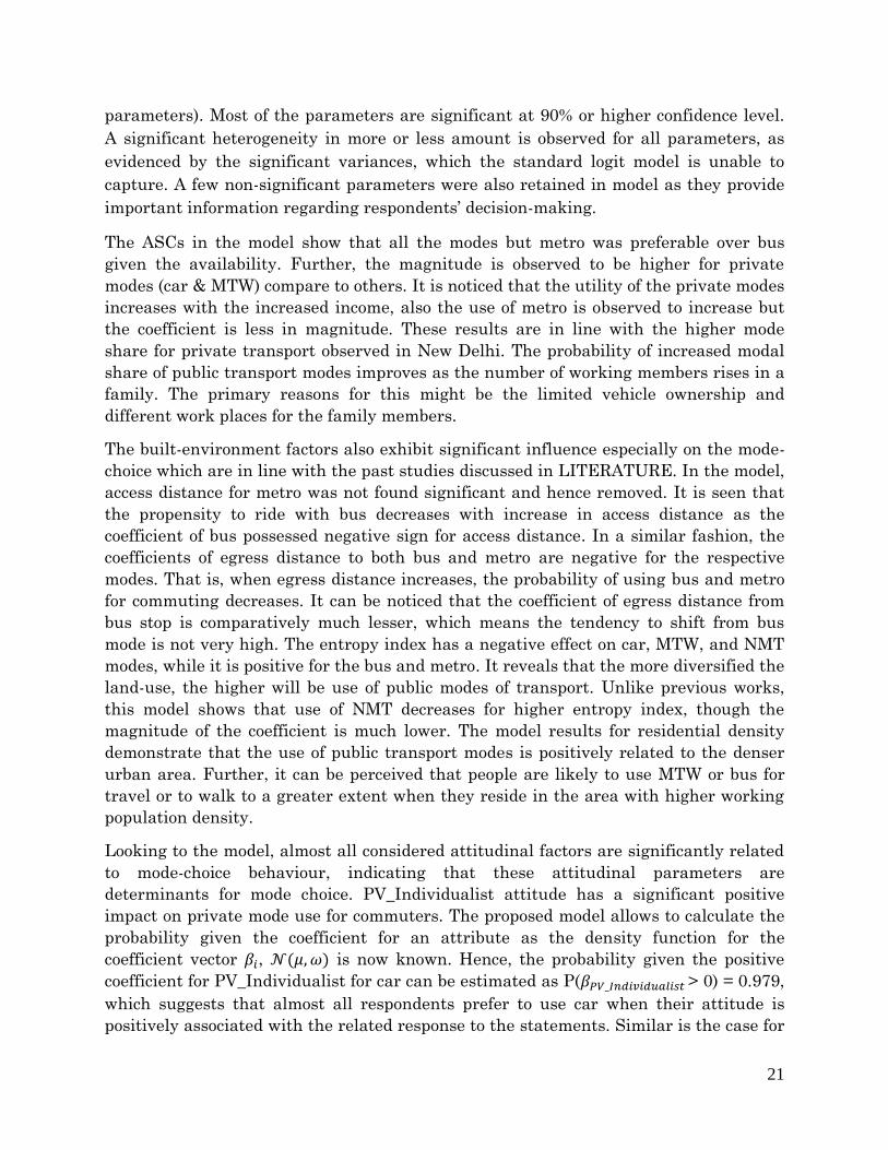
MTW mode. In contrary, the awareness on environmental concerns causes negative
effects on both the private modes, but the magnitude of coefficient is higher for car. It
dictates that the use of car is substantially dependent on the pro-environment attitude
(P(𝛽𝑃𝑉_𝑃𝑟𝑜−𝑒𝑛𝑣𝑖𝑟𝑜𝑛𝑚𝑒𝑛𝑡 < 0) = 0.712). It can be noted that commuting by MTW is positively
related to the attitude of economy. It reveals respondents are less concerned about
economic aspects since the current levels of travel cost and parking fees are
comparatively much lesser for MTW. The attitude related to the travel comfort is
positively associated with the choice of private modes and supports the statements for
the same. Flexibility has overall negative effect on the car use given the higher
covariances for Flexibility2 and Flexibilty3 (Table 2). The model also suggests that car
users put more weightage on safety while selecting parking type. Conversely, MTW
users consider convenience as more important compare to safety. The related
probabilities are estimated as: P(𝛽𝑃𝑎𝑟𝑘𝑛𝑔_𝑆𝑎𝑓𝑒𝑡𝑦 > 0) = 0.999 for Car_Off; P(𝛽𝑃𝑎𝑟𝑘𝑛𝑔_𝑆𝑎𝑓𝑒𝑡𝑦 >
0) = 0.857 for MTW_Off; P(𝛽𝑃𝑎𝑟𝑘𝑛𝑔_𝐶𝑜𝑛𝑣𝑒𝑛𝑖𝑒𝑛𝑐𝑒 > 0) = 0.861 for Car_On; and
P(𝛽𝑃𝑎𝑟𝑘𝑛𝑔_𝐶𝑜𝑛𝑣𝑒𝑛𝑖𝑒𝑛𝑐𝑒 > 0) = 0.953 for MTW_On. These state that the parking users with
safety concerns in their mind tend to park their vehicle at off-street parking, whereas
individuals would prefer the on-street parking given their positive attitudes towards
parking convenience.
The results of public transit attitudes are in line with those found in the
LITERATURE. From the association of four attitudes of public transit with bus use, it
is clear that safety followed by convenience are the most detrimental factors for bus
use. It can be observed that the magnitude of mean of coefficients are higher with lower
variance, which shows lesser heterogeneity in decision-making. The probability is
estimated as P(𝛽𝑃𝑇_𝑆𝑎𝑓𝑒𝑡𝑦 < 0) = 0.998 and P(𝛽𝑃𝑇_𝐶𝑜𝑛𝑣𝑒𝑛𝑖𝑒𝑛𝑐𝑒 < 0) = 0.953, which indicates
almost all individuals who confer more importance on these aspects, have a lower use of
bus. Further, the comfort (in negative manner) has positive coefficient for bus indicate
that people give less emphasize to it given their lower cost affordability and lesser
income (particularly who use bus in Delhi). Likewise, safety influence attitudes towards
using metro for commuting though the extent is lower compared to bus. Convenience
and flexibility are related positively with the use of metro, which is in contrary to what
observed for the bus. It shows that keeping other parameters constant, respondents are
more likely to select a metro over bus for commuting given their psychological mindset
for convenience (primarily time-reliability) and flexibility. Further it can be recognized
that respondents give least preference to walking/cycling modes as all the attitudinal
parameters associated with the public transit are negatively related to NMT modes.
Higher and positive 𝛽𝑁𝑀𝑇_𝐻𝑒𝑎𝑙𝑡ℎ confirm that the respondents who are health-concerned
tend to use NMT modes over all other modes given the calculated probability of this
choice being close to 1. It is also found that the more someone perceive NMT a
convenient mode, the more he/she will use NMT for short-distant commute trips. On
the other hand, those who value safety and comfort (in negative manner) feel negatively
towards walking/cycling.
23
Parking and travel parameters possess a considerable impact on individuals’ choice
behaviour. It is observed that the likeliness of using public transport and car increases
for longer trips, whereas people are less likely to use MTW and NMT modes. A quite
higher coefficient of distance for metro compare to other modes (car and bus) indicates
its attractiveness for large distance trips. This finding is supported by an estimate of
average trip length of Delhi metro being approximately 15 km (Goel and Tiwari, 2016).
IVTT and travel cost are negatively associated with the selection of a travel mode.
Coefficient of IVTT for bus has the highest value among the considered modes, which
shows that a small rise in IVTT would have a significant effect on bus being chosen as a
travel mode. Such effect is seen smaller in case of metro looking to the coefficient for
IVTT in metro. Generally, rail-based transit is preferred to avoid inconvenience caused
due to traffic jams on roads and hence such tendency in terms of IVTT makes sense.
The model shows that parking related attributes also have a significant influence in
respondents’ decision-making. Parking search time and parking egress time has
negative coefficients for both the parking types and indicate that the utility decreases
when the value of these variables increases. Also, it is noticed that respondents put
nearly equal importance to both the variables. Parking duration also has a significant
impact on joint mode-parking choice behaviour. It is obvious that people who need to
use a parking for more duration would prefer off-street parking as captured by the
model. Relatively higher magnitude of parking duration for car users (both on street
and off street) shows their higher tendency to shift to off-street parking when parking
duration increases. The Employer-paid parking can be treated as a very deciding factor
for choosing PVs as commute modes as can be seen from the model. Here, only off-street
is considered for employer-paid parking as no related on-street parking was reported in
survey.
5.3. Willingness to pay analysis
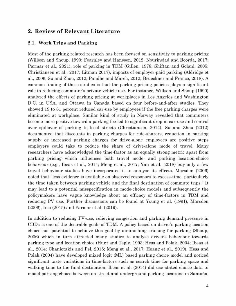
Figure 2 presents the box plot showing the distribution of individual level MWTP
estimates based on the developed mixed model. Please note that the distance is in the
scale of 100 meters and time is in hour. The cross-marks in the box indicate the mean
values of MWTP. Among the accessibility parameters, egress distance to metro clearly
shows the largest MWTP value with less variation, indicating that commuters are more
willing to pay for higher accessible metro at their work place. This is also supported by
the higher coefficient value of attitude towards PT convenience in the model. Further, it
is revealed that the commuters put more value to the egress distance compare to access
distance for both the PT modes. This finding is similar to one observed in meta-analysis
by Ewing and Cervero (2010). Some of the respondents put negative values on MWTP,
which shows that they have to be compensated by the stated amounts (for e.g.,
maximum of ₹1.89 per trip for access distance to bus) in order to add the positivity for
using bus. In case of IVTT, car users are comparatively more willing to pay to reduce
their travel time on an average, followed by bus users. A reasonable explanation for
this is that, car and bus affect more in congestion due to bigger size compared to MTW,
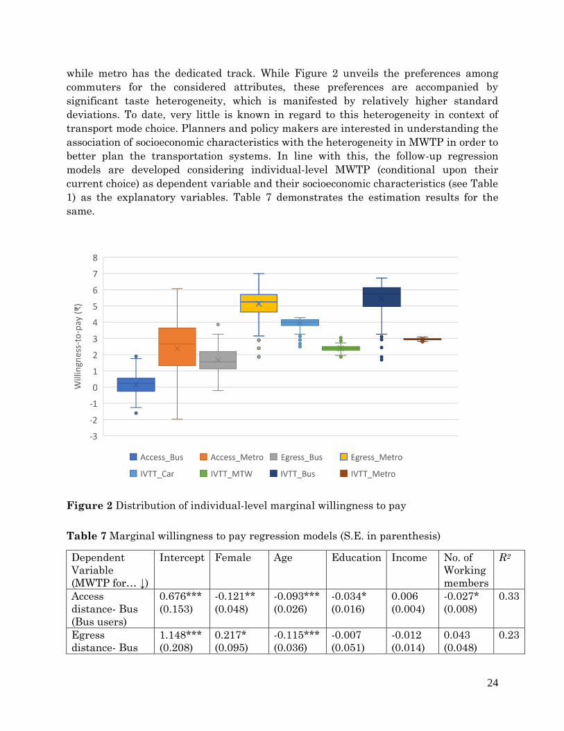
24
while metro has the dedicated track. While Figure 2 unveils the preferences among
commuters for the considered attributes, these preferences are accompanied by
significant taste heterogeneity, which is manifested by relatively higher standard
deviations. To date, very little is known in regard to this heterogeneity in context of
transport mode choice. Planners and policy makers are interested in understanding the
association of socioeconomic characteristics with the heterogeneity in MWTP in order to
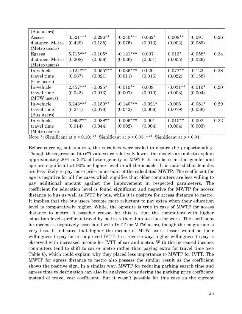
better plan the transportation systems. In line with this, the follow-up regression
models are developed considering individual-level MWTP (conditional upon their
current choice) as dependent variable and their socioeconomic characteristics (see Table
1) as the explanatory variables. Table 7 demonstrates the estimation results for the
same.
Figure 2 Distribution of individual-level marginal willingness to pay
Table 7 Marginal willingness to pay regression models (S.E. in parenthesis)
Dependent
Variable
(MWTP for… ↓)
Intercept Female Age Education Income No. of
Working
members
R2
Access
distance- Bus
(Bus users)
0.676***
(0.153)
-0.121**
(0.048)
-0.093***
(0.026)
-0.034*
(0.016)
0.006
(0.004)
-0.027*
(0.008)
0.33
Egress
distance- Bus
1.148***
(0.208)
0.217*
(0.095)
-0.115***
(0.036)
-0.007
(0.051)
-0.012
(0.014)
0.043
(0.048)
0.23
25
(Bus users)
Access
distance- Metro
(Metro users)
3.521***
(0.429)
-0.296**
(0.135)
-0.240***
(0.075)
0.062*
(0.013)
0.008**
(0.002)
-0.091
(0.089)
0.26
Egress
distance- Metro
(Metro users)
5.715***
(0.208)
-0.105*
(0.056)
-0.121***
(0.036)
0.007
(0.051)
0.013*
(0.005)
-0.058*
(0.026)
0.34
In-vehicle
travel time
(Car users)
4.124***
(0.067)
-0.055***
(0.021)
-0.036***
(0.011)
0.020
(0.016)
0.077**
(0.022)
-0.122
(0.158)
0.28
In-vehicle
travel time
(MTW users)
2.457***
(0.042)
-0.025*
(0.013)
-0.019**
(0.007)
0.009
(0.010)
-0.031**
(0.003)
-0.010*
(0.004)
0.20
In-vehicle
travel time
(Bus users)
6.243***
(0.241)
-0.150**
(0.076)
-0.140***
(0.042)
-0.021*
(0.006)
-0.006
(0.079)
-0.081*
(0.036)
0.29
In-vehicle
travel time
(Metro users)
2.993***
(0.014)
-0.088**
(0.044)
-0.006***
(0.002)
-0.001
(0.004)
0.010**
(0.004)
-0.002
(0.003)
0.22
Note: *: Significant at p < 0.10; **: Significant at p < 0.05; ***: Significant at p < 0.01.
Before carrying out analysis, the variables were scaled to ensure the proportionality.
Though the regression fit (R2) values are relatively lower, the models are able to explain
approximately 20% to 34% of heterogeneity in MWTP. It can be seen that gender and
age are significant at 90% or higher level in all the models. It is noticed that females
are less likely to pay more price in account of the calculated MWTP. The coefficient for
age is negative for all the cases which signifies that older commuters are less willing to
pay additional amount against the improvement in respected parameters. The
coefficient for education level is found significant and negative for MWTP for access
distance to bus as well as IVTT by bus, while it is positive for access distance to metro.
It implies that the bus users become more reluctant to pay extra when their education
level is comparatively higher. While, the opposite is true in case of MWTP for access
distance to metro. A possible reason for this is that the commuters with higher
education levels prefer to travel by metro rather than use bus for work. The coefficient
for income is negatively associated with IVTT for MTW users, though the magnitude is
very less. It indicates that higher the income of MTW users, lesser would be their
willingness to pay for an improved IVTT. In a reverse way, higher willingness to pay is
observed with increased income for IVTT of car and metro. With the increased income,
commuters tend to shift to car or metro rather than paying extra for travel time (see
Table 6), which could explain why they placed less importance to MWTP for IVTT. The
MWTP for egress distance to metro also possess the similar result as the coefficient
shows the positive sign. In a similar way, MWTP for reducing parking search time and
egress time to destination can also be analysed considering the parking price coefficient
instead of travel cost coefficient. But it wasn’t possible for this case as the current
26
parking price structures in the study location are equivalent for both types of parking.
The coefficient for number of working members in family is negatively associated with
MWTP. The possible reason can be identified in integration with household structure.
For example, MWTP for a person from household having five people with two working
members could be lesser than that for a person from household having two people with
both as working members, given that both households have nearly same income.
6. Discussion and Conclusions
This paper investigates commuters’ travel behaviour by considering parking choice as
an endogenous decision within travel mode choice framework. Using the RP data
collected through individual survey, a mixed logit model with hierarchical Bayes
estimator was formulated to examine the relationships between commuters’ subjective
evaluations as well as objective characteristics and their choice behaviour. As the
proposed model has an ability to provide individual-specific parameter estimation
through simulation, it is possible to understand the heterogeneity in respondents’
willingness-to-pay.
Model estimation results show that various psychological factors attributable to the
travel modes and parking types are significant in determining commuters’ choice
behaviour. The model showed that the attitudes towards safety, comfort and
convenience are strong drivers for respondents’ parking choice as well as mode-shift
decisions in general. Particularly for PVs, individualist attitude is seen to have large
influence on both car and MTW choices. In countries like India, vehicle ownership is
seen as a reflection of the wealth and social status. This in turn encourages individuals
to use their private vehicles given the lack of ample knowledge of sustainability.
Further, there is no policy in place to control the vehicle ownership. Even the parking
charges are very low compared to other similar size cities across the world (MoHUA,
2019). City authorities should focus on these aspects as they are key elements in habit-
breaking (of PV-use). Apart from improving the public transit service quality,
educational program should be organized which can strengthen individuals’ perception
and responsibility towards sustainability. Public transit users place highest importance
to safety and convenience (in terms of accessibility) and hence, it should be of utmost
importance to planning authorities also to promote the PT use. The lower-income group
tend to live farther from the city center and CBDs. They don’t have much viable
transport options but to use MTW for commute because of non-affordability of car and
poor first/last mile connectivity issues with transit, which is also confirmed by this
study. These is the primary reason for higher MTW ownership in developing countries.
The choice model shows that rise in access/egress distance make transit modes less
attractive. Willingness-to-pay analysis shows the significance of access/egress
characteristics on selection of main transport mode. Hence, due consideration should be
given to improve last-mile connectivity of public transport modes. Increasing coverage
of public transit seem to be a solution to address this issue. Practically, it is difficult to
provide fixed-guideway mass transit (like metro) in all areas of the city due to higher
27
marginal costs. Hence, such area should be facilitated by lower category of transit
service like bus, regulated para-transit service. Apart from this, providing efficient
feeder services can confine the existing transit users escaping from using the service
and attract private vehicle users towards transit. In addition, integration of PT system
(bus + metro in this case) in terms of schedule, fare, and stops seem to increase the PT
ridership as it can effectively compete with private vehicles usage (Zimmerman and
Fang, 2015). Such integration with common mobility fare card and well-organized
feeder-service may prove to be a promising action for promoting PT.
The model results illustrate key findings for NMT-use: all four latent variables –
health, safety, comfort and convenience – have strong impacts on peoples’ intention to
use NMT. In most Indian cities including Delhi, a common problem is observed that the
sidewalks are generally occupied by the vendors and in poor condition at many
locations forcing pedestrians to get down on the carriageway. Also, bicyclists generally
ride in mixed traffic due to absence of dedicated path or hindrance by vendors (if
present) which declines bicycle-usage significantly. Policy interventions have to be
focused on improving peoples’ satisfaction which may in turn improve the NMT share.
The educational program focusing on coexistence of transport modes might be
accompanied with these interventions for better outcomes. The Street Vending Policy
should appropriately address the vending management in cities to overcome the stated
issues. The guidelines published in Tender S.U.R.E. (Specifications for Urban Road
Execution) and implemented in the city of Bangalore can be considered in this line
(Ramanathan, 2011).
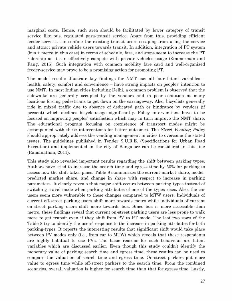
This study also revealed important results regarding the shift between parking types.
Authors have tried to increase the search time and egress time by 50% for parking to
assess how the shift takes place. Table 8 summarizes the current market share, model-
predicted market share, and change in share with respect to increase in parking
parameters. It clearly reveals that major shift occurs between parking types instead of
switching travel mode when parking attributes of one of the types rises. Also, the car
users seem more vulnerable to these changes compared to MTW users. Individuals of
current off-street parking users shift more towards metro while individuals of current
on-street parking users shift more towards bus. Since bus is more accessible than
metro, these findings reveal that current on-street parking users are less prone to walk
more to get transit even if they shift from PV to PT mode. The last two rows of the
Table 8 try to identify the users’ response to the increase in parking attributes for both
parking-types. It reports the interesting results that significant shift would take place
between PV modes only (i.e., from car to MTW) which reveals that these respondents
are highly habitual to use PVs. The basic reasons for such behaviour are latent
variables which are discussed earlier. Even though this study couldn’t identify the
monetary value of parking search time and egress time, these results can be used to
compare the valuation of search time and egress time. On-street parkers put more
value to egress time while off-street parkers to the search time. From the combined
scenarios, overall valuation is higher for search time than that for egress time. Lastly,
28
no shift is seen towards NMT modes except when parking search time increases. These
group of respondents may not be willing to spend much time to search for vacant
parking place as they travel for much lesser time between origin and destination.
Table 8 Change in market share (%) under different scenarios
Scenario Car_Off Car_On MTW_Off MTW_On Bus Metro NMT
Current market
share 17.28 7.64 11.30 13.95 24.58 16.61 8.64
Predicted market
share 18.37 6.54 9.88 15.37 24.58 16.62 8.64
Increase off-street
parking search time -2.35 1.60 -1.77 1.48 0.37 1.10 0.00
Increase on-street
parking search time 0.54 -1.52 0.40 -0.91 0.27 0.20 0.00
Increase on-street
parking egress time 0.87 -2.45 1.01 -1.41 0.30 0.25 0.00
Increase off-street
parking egress time -1.74 1.58 -1.16 1.07 0.37 0.45 0.00
Increase parking
egress time for both
types
-1.66 -1.37 1.03 0.31 0.53 0.69 0.00
Increase parking
search time for both
types
-1.84 -1.95 0.45 0.47 0.75 0.95 0.08
Another important observation from the present study is the positive association of
employer-paid parking with PV-use. It can create hindrance in attaining sustainability
if there are no counter policies like parking cash-out or mass transit subsidies
established alongside. The related concerns are well discussed by Shoup (2005) and
Parmar et al. (2021). As a policy measure, urban local bodies may introduce parking
credit system for encouraging PV users to utilize PT system for select work trips of the
week. For such trips, the PV users can earn parking credit points which may be
encashed against parking charges at sites of higher parking cost (e.g., shopping areas).
This may gradually improve the PT modal share for commute trips. Moreover,
appropriate parking fare structure including differential parking pricing for on-street
and off-street lots should be formulated to effectively manage the parking supply as
well as to confront the serious on-street parking issues. Though there is a less room for
intentional changes in parking search time and egress time compared to parking
pricing, building remote parking lots in the peripheral parts of CBDs with proper
integration with transit in inner parts can be considered as a long-term sustainable
solution.
29
In general, this study provides important evidence on how commuters’ attitudes and
built-environment can act as decisive factors in determining their travel mode and
parking-type choice. It should be noted that the model results and MWTP values could
not be directly compared to developed countries just like rapidly urbanizing developing
countries in south Asia as income and population densities play major roles in this case.
To overcome the limitations related to parking cost in this study, a combined
framework of RP-SP survey data should be deployed to assess commuters’ response to
various parking pricing policies in addition to other attributes.
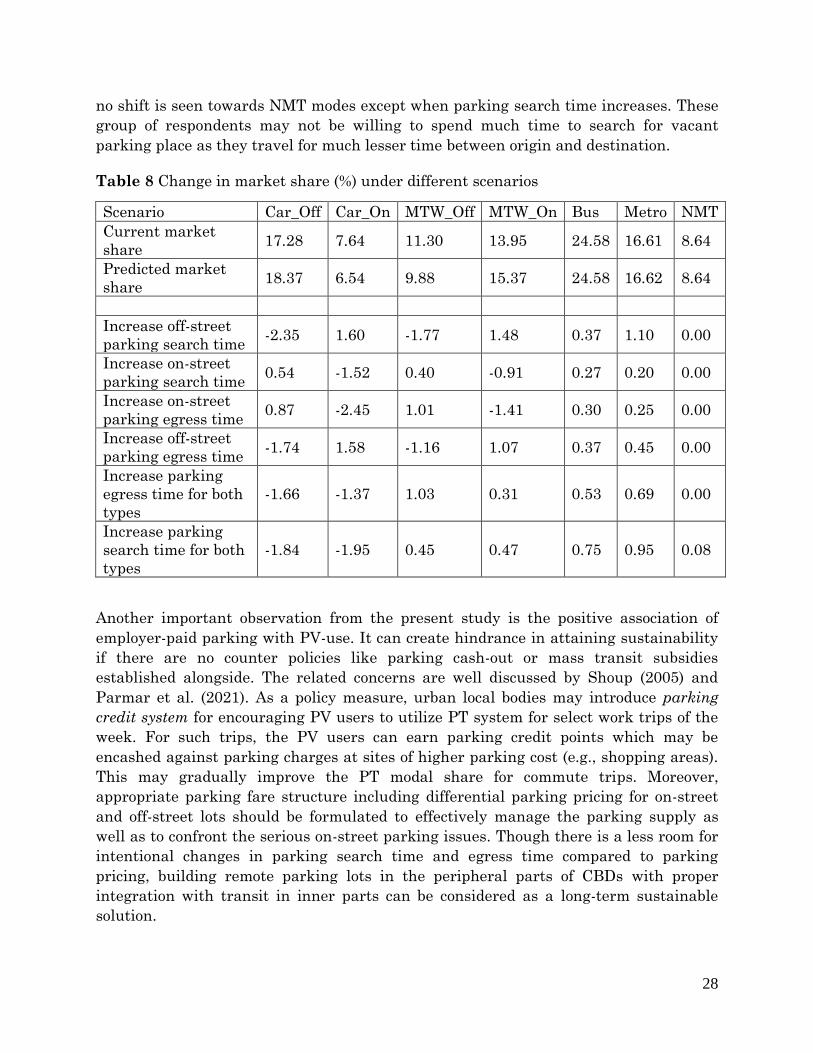
APPENDIX
Table A1 Indicators for latent variables for private vehicles
Latent
Variable
Indicator
Individualist
Individualist1. I have social status. I will use my vehicle only.
Individualist2. I can afford PV and related costs. Why should I go for
PT!!
Individualist3. Driving is fun and relaxing.
Individualist4. Driving to destination provides safety and privacy
compare to other alternatives.
Pro-
environment
Pro-environment1. Private vehicles are the reason for congestion and
pollution.
Pro-environment2. I can contribute to make difference on
environmental problems.
Pro-environment3. People should be made aware of environmental
concerns.
Economy
Economy1. Higher tax should be levied from PV users against
congestion.
Economy2. The fuel price should be increased to limit PV-use.
Economy3. Parking fees should be high to limit PV-use.
Comfort
Comfort1. Crowding and comfort are main reasons why I prefer PV over
PT.
Comfort2. Using PV is time saving and reliable.
Flexibility
Flexibility1. PV offers flexibility of choosing route and I can make
multiple stops if required.
Flexibility2. It is difficult to find parking space nowadays.
Flexibility3. Looking to congestion, I worry to be on time at my
destination while using my car.
30
Table A2 Indicators for latent variables for public transport
Latent
Variable
Indicator
Comfort
Comfort1. Crowding and comfort are main reasons why I prefer PV over
PT.
Comfort2. It is annoying to take multiple stops/transfers while
travelling by PT.
Comfort3. Waiting for bus is annoying.
Comfort4. Taking PT is difficult when I travel with bags/luggage.
Convenience
Convenience1. We need more accessible PT to limit PV-use.
Convenience2. I am not sure whether I will be on time to my destination
while traveling by Bus.
Convenience3. I will be on time if travel by Metro.
Safety
Safety1. Lesser chances of accidents if we use PT.
Safety2. PT (including stops) is not safe from theft when comparing
with other alternatives.
Safety3. I do not like to be surrounded by unknown people.
Flexibility
Flexibility1. Services (like shops and food stalls) make waiting more
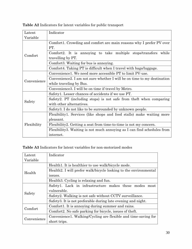
pleasant.
Flexibility2. Getting a seat from time-to-time is not my concern.
Flexibility3. Waiting is not much annoying as I can find schedules from
internet.
Table A3 Indicators for latent variables for non-motorized modes
Latent
Variable
Indicator
Health
Health1. It is healthier to use walk/bicycle mode.
Health2. I will prefer walk/bicycle looking to the environmental
issues.
Health3. Cycling is relaxing and fun.
Safety
Safety1. Lack in infrastructure makes these modes most
vulnerable.
Safety2. Walking is not safe without CCTV surveillance.
Safety3. It is not preferable during late evening and night.
Comfort Comfort1. It is annoying during summer and rains.
Comfort2. No safe parking for bicycle, issues of theft.
Convenience Convenience1. Walking/Cycling are flexible and time-saving for
short trips.
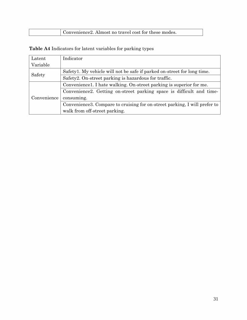
31
Convenience2. Almost no travel cost for these modes.
Table A4 Indicators for latent variables for parking types
Latent
Variable
Indicator
Safety Safety1. My vehicle will not be safe if parked on-street for long time.
Safety2. On-street parking is hazardous for traffic.
Convenience
Convenience1. I hate walking. On-street parking is superior for me.
Convenience2. Getting on-street parking space is difficult and time-
consuming.
Convenience3. Compare to cruising for on-street parking, I will prefer to
walk from off-street parking.
32
References
Abrahamse, W., Steg, L., Gifford, R., Vlek, C., 2009. Factors influencing car use for
commuting and the intention to reduce it: A question of self-interest or morality?
Transp. Res. Part F: Traffic Psychol. Behav. 12, 317–324.
Albert, G., Mahalel, D., 2006. Congestion tolls and parking fees: a comparison of the
potential effect on travel behaviour. Transp. Policy 13, 496–502.
Aldridge, K., Carreno, M., Ison, S., Rye, T., Straker, I., 2006. Car parking management
at airports: a special case? Parking. Transport Policy 13 (6), 511–521.
Brueckner, J.K., Franco, S.F., 2018. Employer-paid parking, mode choice, and
suburbanization. Journal of Urban Economics, 104, 35–46.
Campbell, D., 2007. Willingness to pay for rural landscape improvements: combining
mixed logit and random-effects models. Journal of Agricultural Economics. 58(3),
467-483.
Cao, X., Mokhtarian, P.L., Handy, S.L., 2009. Examining the impacts of residential self-
selection on travel behaviour: a focus on empirical findings. Transp. Rev. 29(3),
359-395.
Cervero, R., Radisch, C., 1996. Travel choices in pedestrian versus automobile oriented
neighborhoods. Transp. Policy 3, 127–141.
Chaniotakis, E., Pel, A. J., 2015. Drivers’ parking location choice under uncertain
parking availability 33 and search times: A stated preference experiment. Transp.
Res. Part A Policy Pract., 82, 228-239.
Chidambaram, B., Janssen, M. A., Rommel, J., Zikos, D., 2014. Commuters’ mode
choice as a coordination problem: A framed field experiment on traffic policy in
Hyderabad, India. Transp. Res. Part A Policy Pract., 65, 9-22.
Christiansen, P., 2014. A case study of parking charges at work places – effects on
travel behaviour and acceptance. In: Selected Proceedings from the Annual
Transport Conference at Aalborg University.
Christiansen, P., Engebretsen, Ø., Fearnley, N., Usterud Hanssen, J., 2017. Parking
facilities and the built environment: Impacts on travel behaviour. Transp. Res.
Part A Policy Pract. 95, 198–206.
Directorate of Economics & Statistics, Govt. of NCT of Delhi. “Delhi Statistical
Handbook 2020.” January 2021. http://www.des.delhigovt.nic.in/
ECMT, 2004. In: Assessment and Decision Making for Sustainable Transport.
European Conference of Ministers of Transportation, Organization of Economic
Coordination and Development. www.oecd.org
Engebretsen, Ø., Christiansen, P., 2011. Bystruktur og transport. En studie av
personreiser i byer og tettsteder. TØI-rapport 1178/2011
33
Etminani-Ghasrodashti, R., Ardeshiri, M., 2015. Modeling travel behavior by the
structural relationships between lifestyle, built environment and non-working
trips. Transp. Res. Part A Policy Pract., 78, 506-518.
Evangelinos, C., Tscharaktschiew, S., Marcucci, E., Gatta, V., 2018. Pricing workplace
parking via cash-out: Effects on modal choice and implications for transport
policy. Transp. Res. Part A Policy Pract., 113, 369–380.
Ewing, R., Cervero, R., 2010. Travel and the built environment: a meta-analysis. J. Am.
Plan. Assoc. 76(3), 265-294.
Fearnley Nils, Hanssen Jan Usterud, 2012. Basic Data about Urban Parking and
Parking Price Elasticity. TOI Report 1206/2012
Frank, L., Bradley, M., Kavage, S., Chapman, J., Lawton, T.K., 2008. Urban form,
travel time, and cost relationships with tour complexity and mode choice.
Transportation, 35(1), 37-54.
Gillen, D.W., 1978. Parking policy, parking location decisions and distribution of
congestion. Transportation 7 (1), 69–85.
Goel, R., Tiwari, G., 2016. Access–egress and other travel characteristics of metro users
in Delhi and its satellite cities. IATSS Research. 39(2), 164-172.
Golias, J., Yannis, G., Harvatis, M., 2002. Off-street parking choice sensitivity. Transp.
Plan. Technol. 25 (4), 333–348.
Guan, X., & Wang, D., 2019. Influences of the built environment on travel: A household-
based perspective. Transp. Res. Part A Policy Pract., 130, 710–724.
Guan, X., Wang, D. 2019. Influences of the built environment on travel: A household-
based perspective. Transp. Res. Part A Policy and Pract., 130, 710–724.
Han, Y., Li, W., Wei, S., Zhang, T., 2018. Research on Passenger’s Travel Mode Choice
Behavior Waiting at Bus Station Based on SEM-Logit Integration Model.
Sustainability. 10(6), 1996.
Hess, S., Polak, J.W., 2004. Mixed logit estimation of parking type choice. In: 83rd
Annual Meeting of the Transportation Research Board. Washington, DC.
Hoang, P.H., Zhao, S., Houn, S.E., 2019. Motorcycle Drivers’ Parking Lot Choice
Behaviors in Developing Countries: Analysis to Identify Influence Factors.
Sustainability, 11(9), 2463.
Hoshino, T., 2011. Estimation and analysis of preference heterogeneity in residential
choice behaviour. Urban Studies. 48(2), 363-382.
Hunt, J.D., Teply, S., 1993. A nested logit model of parking location choice. Transp. Res.
27B, 253–265.
Ibeas, A., dell’Olio, L., Bordagaray, M., Ortúzar, J. de D., 2014. Modelling parking
choices considering user heterogeneity. Transp. Res. Part A Policy Pract., 70, 41–
49.
Inci, E. 2015. A review of the economics of parking. Economics of Transportation, 4(1-2),
50-63.
34
Jackman, S., Estimation and inference are missing data problems: unifying social
science via Bayesian simulation. Political Analysis. 8(4), 307-332.
Lenk, P., 2014. Bayesian estimation of random utility models, in: Handbook of Choice
Modelling. Edward Elgar Publishing. 457-497.
Litman, T., 2017. Sustainable Transportation and TDM: Planning that Balances
Economic, Social and Ecological Objectives. Victoria Transport Policy Institute.
http://www.vtpi.org/tdm/tdm67.htm
Marsden, G. 2006. The evidence base for parking policies—a review. Transport policy,
13(6), 447-457
Meng, F., Du, Y., Chong Li, Y. and Wong, S.C., 2018. Modeling heterogeneous parking
choice behavior on university campuses. Transp. Plan. Technol., 41(2), 154-169.
Milosavljevic, N., Simicevic, J., 2019. Parking Strategy. In: Sustainable Parking
Management: Practices, Policies and Metrics. pp. 139-163. Elsevier.
Ministry of Road Transport and Highways (MoRT&H), India, 2018. Open Government
Data (OGD) platform India. https://www.data.gov.in/ (Accessed 6 November 2018).
Muthén B. O., 1984. A general structural equation model for dichotomous, ordered
categorical and continuous latent variable indicators. Psychometrika. 49, 115–132.
Naess, P., 2012. Urban form and travel behaviour: experience from a Nordic context. J.
Transp. Land Use 5(2), 21-45.
Nourinejad, M., Roorda, M.J., 2017. Impact of hourly parking pricing on travel demand.
Transp. Res. Part A Policy Pract., 98, 28-45.
Pandhe, Amruta, March, Alan, 2012. Parking availability influences on travel mode:
Melbourne CBD offices. Austral. Plan. 49 (2), 161–171.
Parmar, J., Das, P., Dave, S.M. (2021). A machine learning approach for modelling
parking duration in urban land-use. Physica A: Statistical Mechanics and its
Applications. 572, 125873.
Parmar, J., Das, P., Dave, S.M., 2019. Study on demand and characteristics of parking
system in urban areas: A review. J. Traffic Transp. Eng. (Engl. Ed.), 7(1), 111-124.
Paulssen, M., Temme, D., Vij, A., & Walker, J. L., 2013. Values, attitudes and travel
behavior: a hierarchical latent variable mixed logit model of travel mode choice.
Transportation, 41(4), 873–888.
Planning Department, Government of Delhi. "Gross State Domestic Product of Delhi".
pg. 16. Retrieved 9 June 2019.
http://delhiplanning.nic.in/sites/default/files/Budget%202019-
20_English%20for%20CM.pdf
Planning Department, Govt. of NCT of Delhi. “Economic Survey of Delhi 2018-19.”
2019. http://delhiplanning.nic.in/content/economic-survey-delhi-2018-19
Rahul, T.M., Verma, A. 2017. The influence of stratification by motor-vehicle ownership
on the impact of built environment factors in Indian cities. J. Transp. Geogr., 58,
40–51.
35
Ramanathan, S. (2011). Tender S.U.R.E. (Specifications for Urban Road Execution)
Volume I. https://www.janausp.org/wp-content/uploads/2021/02/tendersure-
vol1.pdf
Rhemtulla, M., Brosseau-Liard, P. É., & Savalei, V., 2012. When can categorical
variables be treated as continuous? A comparison of robust continuous and
categorical SEM estimation methods under suboptimal conditions. Psychological
methods. 17, 354-373.
Richardson, B., 1999. Towards a policy on a sustainable transportation system.
Transportation Research Record. 1670, 27–34.
Rye, T., Cowan, T., Ison, S., 2006. Expansion of a controlled parking zone (CPZ) and its
influence on modal split: the case of Edinburgh. Transp. Plan. Technol. 29(1), 75–
89.
Sanit, P., Nakamura, F., Tanaka, S., Wang, R., 2013. Location and Mode Choice
Decision Mechanism Analysis of Multi-Worker Household in Bangkok, Thailand.
(In the Proceedings of the Eastern Asia Society for Transportation Studies 9).
Shiftan, Y., Golani, A., 2005. Effect of Auto Restraint Policies on Travel Behavior 1932,
156–163.
Shoup, D., 2005. The high cost of free parking. Planners Press.
Shoup, D., 2006. Cruising for parking. Transport Policy. 13(6), 479-486.
Steg, L., Kalfs, N., 2000. Altijd weer die auto. Sociaal en Clutureel
Planbureau/Adviesdienst Verkeer en Vervoer, The Hague.
Su, Q., Zhou, L., 2012. Parking management, financial subsidies to alternatives to drive
alone and commute mode choices in Seattle. Reg. Sci. Urban Econ. 42 (1–2), 88–
97.
The Boston Consulting Group, 2018. Unlocking Cities: The impact of ridesharing across
India. http://image-src.bcg.com/Images/BCG-Unlocking-Cities-Ridesharing-
India_tcm9-185213.pdf
Train, K., 2009. Discrete Choice Methods with Simulation. Cambridge University
Press.
Van Acker, V., Mokhtarian, P. L., Witlox, F., 2014. Car availability explained by the
structural relationships between lifestyles, residential location, and underlying
residential and travel attitudes. Transp. Policy, 35, 88–99.
Van Wee, B., Annema, J.A., Banister, D. (Eds.), 2013. The Transport System and
Transport Policy: An Introduction. Edward Elgar, Cheltenham, UK/
Northampton, Massachusetts.
Willson, R. W., & Shoup, D. C. 1990. Parking subsidies and travel choices: assessing the
evidence. Transportation, 17(2), 141-157.
Young, W., Thompson, R. G., & Taylor, M.A. 1991. A review of urban car parking
models. Transport reviews, 11(1), 63-84.
36
Yue, Y., Zhuang, Y., Yeh, A.G.O., Xie, J.-Y.,Ma, C,-L, Li, Q.-Q, 2016. Measurement of
POI-based mixed use and their relationships with neighborhood vibrancy. Int. J.
Geograp. Inform. Sci. 31, 658-675.
Zegras, P.C., Srinivasan, S., 2006. Household Income, Travel Behavior, Location and
Accessibility: Sketches from Two Different Developing Contexts. Transport. Res.
Rec.: J. Transport. Res. Board, 2038(1), 128-138.
Zimmerman, S., and Fang, K. (2015). Public Transport Service Optimization and
System Integration. China Transport Topics, no. 14. World Bank. Washington
D.C.