September 2, 2010. AOS Accounts Payable Update AOS Vendor Processes AOS General Ledger Questions 2.

Analysis of Structures
Book of Examples2018
University of Duisburg-Essen
Faculty of Engineering
Department of Civil Engineering
Structural Analysis of Plate and Shell Structures
Dr. E. Baeck
8.5.2018


Contents
I Programming with Python 3
1 How to get started with Python 51.1 What is Python? . . . . . . . . . . . . . . . . . . . . . . . . . . . . . . . . . . . . . . . 5
1.2 Python, Packages, Utilities . . . . . . . . . . . . . . . . . . . . . . . . . . . . . . . . . 6
1.2.1 Installing the Kernel . . . . . . . . . . . . . . . . . . . . . . . . . . . . . . . . 6
1.2.2 Installing the ComType Package . . . . . . . . . . . . . . . . . . . . . . . . . . 6
1.2.3 Installing the NumPy Package . . . . . . . . . . . . . . . . . . . . . . . . . . . 7
1.2.4 Installing the SciPy Package . . . . . . . . . . . . . . . . . . . . . . . . . . . . 9
1.2.5 Creating Python Source Code . . . . . . . . . . . . . . . . . . . . . . . . . . . 10
1.2.6 Python Implementations . . . . . . . . . . . . . . . . . . . . . . . . . . . . . . 11
1.2.6.1 CPython the Reference Implementation . . . . . . . . . . . . . . . . . 11
1.2.6.2 Jython, let’s go Java . . . . . . . . . . . . . . . . . . . . . . . . . . . 11
1.2.6.3 IronPython, let’s go .Net . . . . . . . . . . . . . . . . . . . . . . . . . 11
1.2.6.4 PyPy, Python to the Square . . . . . . . . . . . . . . . . . . . . . . . 11
1.3 Hello World . . . . . . . . . . . . . . . . . . . . . . . . . . . . . . . . . . . . . . . . . 12
1.4 Python Calculator . . . . . . . . . . . . . . . . . . . . . . . . . . . . . . . . . . . . . . 13
2 Basics in Python 152.1 Code Convention . . . . . . . . . . . . . . . . . . . . . . . . . . . . . . . . . . . . . . 15
2.2 Reserved Words . . . . . . . . . . . . . . . . . . . . . . . . . . . . . . . . . . . . . . . 16
2.3 Packages and Modules . . . . . . . . . . . . . . . . . . . . . . . . . . . . . . . . . . . 16
2.3.1 Import of a whole Module or Package . . . . . . . . . . . . . . . . . . . . . . . 16
2.3.2 Import all Names of a Module . . . . . . . . . . . . . . . . . . . . . . . . . . . 17
2.3.3 Selective Import of Module Names . . . . . . . . . . . . . . . . . . . . . . . . 17
2.3.4 Import with new Names . . . . . . . . . . . . . . . . . . . . . . . . . . . . . . 17
2.4 Operators . . . . . . . . . . . . . . . . . . . . . . . . . . . . . . . . . . . . . . . . . . 18
2.4.1 Unary Operators . . . . . . . . . . . . . . . . . . . . . . . . . . . . . . . . . . 18
2.4.2 Arithmetic Operators . . . . . . . . . . . . . . . . . . . . . . . . . . . . . . . . 18
2.4.3 Bit Operators . . . . . . . . . . . . . . . . . . . . . . . . . . . . . . . . . . . . 19
2.4.4 Extended Assign Operators . . . . . . . . . . . . . . . . . . . . . . . . . . . . . 19
2.4.5 Manipulating Bits and Hexadecimal Numbering System . . . . . . . . . . . . . 20
2.4.6 Comparison Operators . . . . . . . . . . . . . . . . . . . . . . . . . . . . . . . 21
2.4.7 Membership Operators . . . . . . . . . . . . . . . . . . . . . . . . . . . . . . . 22
2.4.8 Identity Operators . . . . . . . . . . . . . . . . . . . . . . . . . . . . . . . . . 22
2.5 Print and Output Formats . . . . . . . . . . . . . . . . . . . . . . . . . . . . . . . . . . 23
2.6 Basic Data Types . . . . . . . . . . . . . . . . . . . . . . . . . . . . . . . . . . . . . . 24
iii
Page iv Analysis of Structures - SS 15
2.7 Code Blocks . . . . . . . . . . . . . . . . . . . . . . . . . . . . . . . . . . . . . . . . . 25
2.8 Globales . . . . . . . . . . . . . . . . . . . . . . . . . . . . . . . . . . . . . . . . . . . 26
2.9 Loop for Repetitions . . . . . . . . . . . . . . . . . . . . . . . . . . . . . . . . . . . . 27
2.9.1 The Factorial . . . . . . . . . . . . . . . . . . . . . . . . . . . . . . . . . . . . 27
2.9.2 Floating Point Precision . . . . . . . . . . . . . . . . . . . . . . . . . . . . . . 30
2.9.2.1 Description of the Application . . . . . . . . . . . . . . . . . . . . . 30
2.9.2.2 Exercise . . . . . . . . . . . . . . . . . . . . . . . . . . . . . . . . . 30
2.10 Functions . . . . . . . . . . . . . . . . . . . . . . . . . . . . . . . . . . . . . . . . . . 31
2.11 Branches for Decisions . . . . . . . . . . . . . . . . . . . . . . . . . . . . . . . . . . . 32
2.12 Conditional Assignments . . . . . . . . . . . . . . . . . . . . . . . . . . . . . . . . . . 32
2.12.1 How to Solve a Quadratic Equation . . . . . . . . . . . . . . . . . . . . . . . . 32
2.12.1.1 A Flow-Chart . . . . . . . . . . . . . . . . . . . . . . . . . . . . . . 33
2.12.1.2 The Implementation . . . . . . . . . . . . . . . . . . . . . . . . . . . 33
2.13 Function Examples . . . . . . . . . . . . . . . . . . . . . . . . . . . . . . . . . . . . . 35
2.13.1 An Abs-Function with Type-Checking . . . . . . . . . . . . . . . . . . . . . . . 35
2.13.2 The Newton-Algorithm . . . . . . . . . . . . . . . . . . . . . . . . . . . . . . . 36
2.14 Data Sequences . . . . . . . . . . . . . . . . . . . . . . . . . . . . . . . . . . . . . . . 39
2.14.1 Working with Tuples . . . . . . . . . . . . . . . . . . . . . . . . . . . . . . . . 39
2.14.2 Working with Lists . . . . . . . . . . . . . . . . . . . . . . . . . . . . . . . . . 40
2.14.3 Working with Dictionaries . . . . . . . . . . . . . . . . . . . . . . . . . . . . . 42
2.15 Error Handling with Exceptions . . . . . . . . . . . . . . . . . . . . . . . . . . . . . . 42
2.15.1 Syntax Errors . . . . . . . . . . . . . . . . . . . . . . . . . . . . . . . . . . . . 42
2.15.2 Exceptions . . . . . . . . . . . . . . . . . . . . . . . . . . . . . . . . . . . . . 43
2.15.3 Handling Exceptions . . . . . . . . . . . . . . . . . . . . . . . . . . . . . . . . 43
2.15.4 Raise Exceptions . . . . . . . . . . . . . . . . . . . . . . . . . . . . . . . . . . 44
2.16 Random Numbers . . . . . . . . . . . . . . . . . . . . . . . . . . . . . . . . . . . . . . 45
2.17 Date, Time and Timespan . . . . . . . . . . . . . . . . . . . . . . . . . . . . . . . . . . 47
2.18 Working with Files . . . . . . . . . . . . . . . . . . . . . . . . . . . . . . . . . . . . . 49
2.18.1 Open a File . . . . . . . . . . . . . . . . . . . . . . . . . . . . . . . . . . . . . 49
2.18.2 Write Data into a File . . . . . . . . . . . . . . . . . . . . . . . . . . . . . . . . 50
2.18.3 Close a File . . . . . . . . . . . . . . . . . . . . . . . . . . . . . . . . . . . . . 50
2.18.4 Read Data from a Text File . . . . . . . . . . . . . . . . . . . . . . . . . . . . . 50
2.18.5 A Logger-Function . . . . . . . . . . . . . . . . . . . . . . . . . . . . . . . . . 52
2.19 OOP with Classes . . . . . . . . . . . . . . . . . . . . . . . . . . . . . . . . . . . . . . 53
2.19.1 Some UML Diagrams . . . . . . . . . . . . . . . . . . . . . . . . . . . . . . . 53
2.19.2 Implementation of Classes in Python . . . . . . . . . . . . . . . . . . . . . . . 55
2.19.2.1 Class Constructor . . . . . . . . . . . . . . . . . . . . . . . . . . . . 55
2.19.2.2 Class Destructor . . . . . . . . . . . . . . . . . . . . . . . . . . . . . 56
2.19.3 Implementation of a Time Stack Class . . . . . . . . . . . . . . . . . . . . . . . 57
3 Python Projects 613.1 Newton, Step2 . . . . . . . . . . . . . . . . . . . . . . . . . . . . . . . . . . . . . . . . 61
3.2 Profiles, Thin Walled Approach . . . . . . . . . . . . . . . . . . . . . . . . . . . . . . . 67
3.2.1 A General Base Class . . . . . . . . . . . . . . . . . . . . . . . . . . . . . . . . 67
3.2.2 A Node Class . . . . . . . . . . . . . . . . . . . . . . . . . . . . . . . . . . . . 69
E. Baeck

CONTENTS Page v
3.2.3 Testing the Node Class . . . . . . . . . . . . . . . . . . . . . . . . . . . . . . . 703.2.4 An Element Class . . . . . . . . . . . . . . . . . . . . . . . . . . . . . . . . . . 713.2.5 Testing the Element Class . . . . . . . . . . . . . . . . . . . . . . . . . . . . . 733.2.6 A General Profile Class . . . . . . . . . . . . . . . . . . . . . . . . . . . . . . . 753.2.7 The AList Class . . . . . . . . . . . . . . . . . . . . . . . . . . . . . . . . . . 793.2.8 Testing the Profile Class . . . . . . . . . . . . . . . . . . . . . . . . . . . . . . 813.2.9 The U-Profile Class . . . . . . . . . . . . . . . . . . . . . . . . . . . . . . . . . 843.2.10 Testing the UProfile Class . . . . . . . . . . . . . . . . . . . . . . . . . . . . . 853.2.11 The Profile Package . . . . . . . . . . . . . . . . . . . . . . . . . . . . . . . . 873.2.12 A Little Profile Database . . . . . . . . . . . . . . . . . . . . . . . . . . . . . . 88
II Scripting with Abaqus 91
4 Some Aspects and Introduction 934.1 Aspects of the Abaqus GUI . . . . . . . . . . . . . . . . . . . . . . . . . . . . . . . . . 934.2 The Abaqus CAE Module . . . . . . . . . . . . . . . . . . . . . . . . . . . . . . . . . 944.3 A Modeling Chain . . . . . . . . . . . . . . . . . . . . . . . . . . . . . . . . . . . . . 954.4 A little interactive Warm Up Example . . . . . . . . . . . . . . . . . . . . . . . . . . . 96
4.4.1 Create a Database . . . . . . . . . . . . . . . . . . . . . . . . . . . . . . . . . . 964.4.2 Create a Sketch . . . . . . . . . . . . . . . . . . . . . . . . . . . . . . . . . . . 964.4.3 Create a Part . . . . . . . . . . . . . . . . . . . . . . . . . . . . . . . . . . . . 964.4.4 Create and Assign Properties . . . . . . . . . . . . . . . . . . . . . . . . . . . . 974.4.5 Create the Instance, Assign the Part . . . . . . . . . . . . . . . . . . . . . . . . 974.4.6 Create a Load Step . . . . . . . . . . . . . . . . . . . . . . . . . . . . . . . . . 974.4.7 Create Loads and Boundary Conditions . . . . . . . . . . . . . . . . . . . . . . 974.4.8 Create the Mesh . . . . . . . . . . . . . . . . . . . . . . . . . . . . . . . . . . 974.4.9 Create a Job and Submit . . . . . . . . . . . . . . . . . . . . . . . . . . . . . . 98
5 Scripts and Examples 995.1 3 Trusses Script . . . . . . . . . . . . . . . . . . . . . . . . . . . . . . . . . . . . . . . 995.2 U-Girder Script . . . . . . . . . . . . . . . . . . . . . . . . . . . . . . . . . . . . . . . 106
5.2.1 System and Automated Analysis . . . . . . . . . . . . . . . . . . . . . . . . . . 1065.2.2 Scripting and OOP . . . . . . . . . . . . . . . . . . . . . . . . . . . . . . . . . 1075.2.3 Class InputData . . . . . . . . . . . . . . . . . . . . . . . . . . . . . . . . . . 1085.2.4 Class ResultData . . . . . . . . . . . . . . . . . . . . . . . . . . . . . . . . . . 1115.2.5 Class Base . . . . . . . . . . . . . . . . . . . . . . . . . . . . . . . . . . . . . 1125.2.6 Class UGirder . . . . . . . . . . . . . . . . . . . . . . . . . . . . . . . . . . . 1135.2.7 Run the UGirder Code . . . . . . . . . . . . . . . . . . . . . . . . . . . . . . . 122
5.2.7.1 Results of the Linear Static Step . . . . . . . . . . . . . . . . . . . . 1235.2.7.2 Results of the Buckling Step . . . . . . . . . . . . . . . . . . . . . . 1245.2.7.3 Results of the Frequency Step . . . . . . . . . . . . . . . . . . . . . . 126
III Appendix 129
A Some Special Problems 131
8.5.2018
Page vi Analysis of Structures - SS 15
A.1 Modules and Packages . . . . . . . . . . . . . . . . . . . . . . . . . . . . . . . . . . . 131
B Some Theory 133B.1 Section Properties . . . . . . . . . . . . . . . . . . . . . . . . . . . . . . . . . . . . . . 133
B.1.1 The Area of a Profile Section . . . . . . . . . . . . . . . . . . . . . . . . . . . . 133B.1.2 First Moments of an Area . . . . . . . . . . . . . . . . . . . . . . . . . . . . . 133B.1.3 Second Moments of an Area . . . . . . . . . . . . . . . . . . . . . . . . . . . . 134B.1.4 Center of Mass . . . . . . . . . . . . . . . . . . . . . . . . . . . . . . . . . . . 135B.1.5 Moments of Inertia with Respect to the Center of Mass . . . . . . . . . . . . . . 135B.1.6 Main Axis Transformation . . . . . . . . . . . . . . . . . . . . . . . . . . . . . 136
C Some Python IDEs 137C.1 The Aptana - IDE . . . . . . . . . . . . . . . . . . . . . . . . . . . . . . . . . . . . . . 137C.2 The PyCharm - IDE . . . . . . . . . . . . . . . . . . . . . . . . . . . . . . . . . . . . . 138
C.2.1 General Statements . . . . . . . . . . . . . . . . . . . . . . . . . . . . . . . . . 138C.2.2 A Hello-Example . . . . . . . . . . . . . . . . . . . . . . . . . . . . . . . . . . 138
D Conventions 141D.1 The Java Code Conventions . . . . . . . . . . . . . . . . . . . . . . . . . . . . . . . . . 141
E Parallel Computing 143E.1 Threads . . . . . . . . . . . . . . . . . . . . . . . . . . . . . . . . . . . . . . . . . . . 143E.2 A Multi-Processing Pool . . . . . . . . . . . . . . . . . . . . . . . . . . . . . . . . . . 143
E.2.1 A Single Processor Solution . . . . . . . . . . . . . . . . . . . . . . . . . . . . 144E.2.2 A Multi Processor Solution . . . . . . . . . . . . . . . . . . . . . . . . . . . . . 145
F Some Special Abaqus-GUI-Features 147F.1 Viewport Annotations . . . . . . . . . . . . . . . . . . . . . . . . . . . . . . . . . . . . 147
F.1.1 The Legend’s Font Size . . . . . . . . . . . . . . . . . . . . . . . . . . . . . . . 147F.2 Specify View . . . . . . . . . . . . . . . . . . . . . . . . . . . . . . . . . . . . . . . . 149
E. Baeck

CONTENTS Page 1
8.5.2018

Page 2 Analysis of Structures - SS 15
E. Baeck
Part I
Programming with Python
3


1
How to get started with Python
1.1 What is Python?
Figure 1.1:Guido van Rossum
Python is a functional and object orientated computer language. The language’sdevelopment was started by Guido van Rossum, who was working with the Cen-trum voor Wiskunde en Informatica (CWI) in Amsterdam Netherlands, see figure1.1
The name Python has nothing to do with the snake of the same name. The namePython was taken from the British surreal comedy group Monty Python (see figure1.2). Because the Monty Python is hard to symbolize onto an icon, the pythonsnake came into picture and so on all icons and Python symbols today we can seethe snake.
The Python language is highly dynamic, so the language is able for example tocreate it’s source code by itself during runtime. This fact and it’s highly portability are reasons for it’sinterpreted kind.
Figure 1.2: Monty Python
So Pyhton code like Java or C# code too is convertedinto a socalled bytecode. The bytecode then is executedon a virtual machine. It’s a program, which can be seenas virtual processor or an emulator. If such a virtual ma-chine is available on a platform, the bytecode can be ex-ecuted without any adaptions.1 With this advantage ofhighly portability Python comes with the general disad-vantage of interpreted languages, the disadvantage of areally bad performance compared to compiled languageslike FORTRAN or C.
1This is only true, if no platform depended packages like comTypes are used.
5

Page 6 Analysis of Structures - SS 15
1.2 Python, Packages, Utilities
If we start with Python, we should think about the choice of the Python version. Because we will usesome additional Python packages, we should be sure, that this packages are available for the desiredPython version. In the case of our lecture we will select the Python version 2.6, which is properly stableand furthermore all the needed add-on packages are available.
To start from the beginning, we have to download the following packages for windows first. It is rec-ommended to download the windows installer version, if available because this is the easiest kind ofinstallation. The installation procedure should start with the installation of the kernel package.
• python-2.6.4.msiThe installer of the python kernel system 2.6.
• comtypes-0.6.2.win32.exeThe installer of Windows types, which are necessary to use Windows API-calls.
• numpy-1.4.1-win32-superpack-python2.6.exeThe installer of the NumPy package for numerical programming.
• scipy-0.8.0-win32-superpack-python2.6.exeThe installer of the SciPy package for sientific programming.
• matplotlib-0.99.3.win32-py2.6.exeThe installer of the MatPlotLib package. This package we need to get the pylab package.
• pywin32-214.win32-py2.6.exeThe installer of a little nice Python IDE.
1.2.1 Installing the Kernel
The python kernel should be the first package, which is to install, because this installation sets up thePython base folder. Within this folder you can find the folder Lib, which contents a lot of libraries andadditional packages and besides that a further sub folder called site-packages. Add ons are copied intothis folder by their installers or by the install Python script.
The start screen of the Python installer shows the Python version. You can select, whether the setupshould make Python available for all users or not. After clicking next you’ll get within the second formthe possibility to select the base folder of Python. By default Python uses the folder C:\Python26.We overwrite the default and select the Windows standard program folder as starting folder, so we writec:\Programme\Python2623.
The figures 1.3 and 1.4 show the input forms installing the Python kernel.
1.2.2 Installing the ComType Package
If you want to use the Python language on a Windows system, it’s recommended to install the ComTypespackage. This package will give you a simple access to the Windows resources. It can be understood as
2The discussed installation was performed on a German system.3The installation of newer packages is working in the same way.
E. Baeck

1.2. PYTHON, PACKAGES, UTILITIES Page 7
Figure 1.3: Start Screen of the Python Installer and Choice of Base Folder
Figure 1.4: Selection the Features and Starting the Installation
a wrapper layer, an interface layer for the access to Windows DLL-modules. ComTypes can be a help todevelop a software with a proper Windows look and feel.
The installation of the most Python packages will run very simular to the following installation. Thefigures 1.5 show the first and second form of the installation procedure. The first form gives a fewinformation to the package. The second form is usually used to select the Python version. Each installedand supported Python version will be listed in the list box of the second form. You can select the desiredPython version and can go on with the installation procedure clicking the next button.
1.2.3 Installing the NumPy Package
NumPy [2] is the fundamental package for scientific computing in Python. It is a Python library that pro-vides a multidimensional array object, various derived objects (such as masked arrays and matrices), andan assortment of routines for fast operations on arrays, including mathematical, logical, shape manipula-tion, sorting, selecting, I/O, discrete Fourier transforms, basic linear algebra, basic statistical operations,random simulation and much more.
At the core of the NumPy package, is the ndarray object. This encapsulates n-dimensional arrays of
8.5.2018

Page 8 Analysis of Structures - SS 15
Figure 1.5: Start Screen of the Package Installer and Choice of the installed Python Version
homogeneous data types, with many operations being performed in compiled code for performance.4
The installation runs like the installation of the ComTypes package (see figure 1.6).
Figure 1.6: Start Screen of the Package Installer and Choice of the installed Python Version
4For more details see NumPy User Guide available on the info.server.
E. Baeck
1.2. PYTHON, PACKAGES, UTILITIES Page 9
1.2.4 Installing the SciPy Package
SciPy [3] is a collection of mathematical algorithms and convenience functions built on the Numpy ex-tension for Python. It adds significant power to the interactive Python session by exposing the user tohigh-level commands and classes for the manipulation and visualization of data. With SciPy, an inter-active Python session becomes a data-processing and system-prototyping environment rivaling sytemssuch as Matlab, IDL, Octave, R-Lab, and SciLab.
The additional power of using SciPy within Python, however, is that a powerful programming languageis also available for use in developing sophisticated programs and specialized applications. Scientificapplications written in SciPy benefit from the development of additional modules in numerous niche’sof the software landscape by developers across the world. Everything from parallel programming to weband data-base subroutines and classes have been made available to the Python programmer. All of thispower is available in addition to the mathematical libraries in SciPy.5
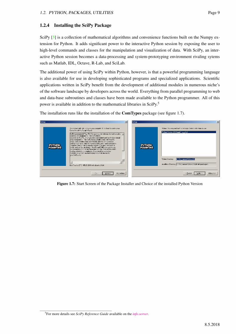
The installation runs like the installation of the ComTypes package (see figure 1.7).
Figure 1.7: Start Screen of the Package Installer and Choice of the installed Python Version
5For more details see SciPy Reference Guide available on the info.server.
8.5.2018

Page 10 Analysis of Structures - SS 15
1.2.5 Creating Python Source Code
To create Python sources we need at least a simple text editor like Notepad++ or PSPad6 like for everycomputer language. This source files with the standard extension py, like helloworld.py, can beexecuted starting the Python interpreter.7
1 c:\pyhton27\python helloworld.py
For Windows there is a lightweigth IDE available called PythonWin. PythonWin looks like an extensionto the MS-Editor Notepad. To create and check small Python scripts, this IDE seems to be ok, becausethe overhead we have to overcome is very small compared to really good IDEs.
The installation of PythonWin runs like the installation of the ComTypes package (see figure 1.8).
Figure 1.8: Start Screen of the PythonWin IDE Installer and Choice of the installed Python Version
After having installed the PythonWin IDE it’s recommended to set up a link onto the desktop (see figure1.9).
Figure 1.9: Creating a Link to the pythonwin.exe
Figure 1.10 shows, how to create a Hello World application in Python and the application’s execution.Within the editor window, we write the source code. With the start button (black triangle) we can run theHello World from the PythonWin. The applications screen output is written into the Interactive Window,which also is working as a Python console.
6Notepad++ and PSPad are available on the info.server in /Software/Editors.7In this case the Python 2.7 was installed into the Folder c:/Python27.
E. Baeck

1.2. PYTHON, PACKAGES, UTILITIES Page 11
Figure 1.10: Creating and Executing a Pyhton Hello within PythonWin
1.2.6 Python Implementations
1.2.6.1 CPython the Reference Implementation
There is not only one Python implementation available. The original implementation is written in C. It’sthe reference implementation, developed by Guido van Rossum, called CPython too.
1.2.6.2 Jython, let’s go Java
Jython (or JPython) is an implementation of the Python language in Java. The interpreter therefor isrunning on a Java environment and is able to use all Java libraries.
1.2.6.3 IronPython, let’s go .Net
IronPython is an implementation for the Common-Language-Infrastructure (CLI), i.e. for the .Net en-vironment on Windows or for the compatible environment Mono on Linux. IronPython is written in C#and is available in a CLI language (like C#) as a script language. IronPython is compatilble to CPython’sversion 2.7.
1.2.6.4 PyPy, Python to the Square
PyPy is a Python interpreter, which is implemented using the Python language. It’s used as an experi-mental environment to develop new features.
8.5.2018

Page 12 Analysis of Structures - SS 15
1.3 Hello World
Like in every computer language there is a Hello World application in Python also possible. We startdhe PythonWin IDE and create a new file. We save this file as HelloWorld.py. With Ctrl-R the executionform is shown and the execution mode should be selected (see figure 1.11).
The following available execution modes are available.
• No debugging,execution without debugging.
• Step-through in the debugger,the debugger is stated and starts with the first statement.
• Run in the debugger,the script is started. Execution is only interrupted at the first breakpoint.
• Post-Mortem of unhandled led exceptions,the debugger is started, if the script crashes with a unhandled exception.
Figure 1.11: Executing the HelloWorld.py Script
If the HelloWorld.py script is executed, the output is written into the Interactive Window, see figure 1.10.
E. Baeck
1.4. PYTHON CALCULATOR Page 13
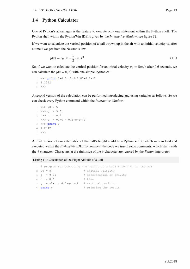
1.4 Python Calculator
One of Python’s advantages is the feature to execute only one statement within the Python shell. ThePython shell within the PythonWin IDE is given by the Interactive Window, see figure ??.
If we want to calculate the vertical position of a ball thrown up in the air with an initial velocity v0 aftera time t we get from the Newton’s law
y(t) = v0 · t−1
2· g · t2 (1.1)
So, if we want to calculate the vertical position for an initial velocity v0 = 5m/s after 0,6 seconds, wecan calculate the y(t = 0, 6) with one simple Python call.
1 >>> print 5*0.6 -0.5*9.81*0.6**2
2 1.2342
3 >>>
A second version of the calculation can be performed introducing and using variables as follows. So wecan check every Python command within the Interactive Window.
1 >>> v0 = 5
2 >>> g = 9.81
3 >>> t = 0.6
4 >>> y = v0*t - 0.5*g*t**2
5 >>> print y
6 1.2342
7 >>>
A third version of our calculation of the ball’s height could be a Python script, which we can load andexecuted within the PythonWin IDE. To comment the code we insert some comments, which starts withthe # character. Characters at the right side of the # character are ignored by the Python interpreter.
Listing 1.1: Calculation of the Flight Altitude of a Ball
1 # program for computing the height of a ball thrown up in the air
2 v0 = 5 # initial velocity
3 g = 9.81 # acceleration of gravity
4 t = 0.6 # time
5 y = v0*t - 0.5*g*t**2 # vertical position
6 print y # printing the result
8.5.2018

Page 14 Analysis of Structures - SS 15
E. Baeck
2
Basics in Python
2.1 Code Convention
In modern programming languages we can use nearly arbitrary names for variables, for functions, classesand packages. Of course the names should be clear, i.e. the should not ambiguous. Sometimes howeverit’s helpful to select names according to a name convention. If we use a name convention, we can put anadditional information into an item’s name, so that a developer can get this information without knowingthe details behind the code.
One of the first conventions was introduced by Charles Simonyi, a Hungarian software engineer, whoworked at Xerox PARC and later with Microsoft. This convention therefore is called Hungarian Notation.The Hungarian Notation inspired from FORTRANs implicit name convention too, introduces some nameprefixes, which should show the developer some information about the variable usage.
With the emergence of the language Java a new code convention was introduced, which today is used inmany applications, so for example in the implementation of the Abaqus Python Interface. This we willdiscuss in the second part (II). A short extract from this code convention, published by Sun Microsystems,Inc. in 1997, we see in the appendix D.1.
From the Java Code Convention we use the following aspects.
1. Variable names will start with small letters.
2. Function names will start with small letters.
3. Class names will start with capital letters.
4. If names consists of several parts, we introduce every part except the first with a capital letter. Thisis called camelCase, because of the shape of the camel’s back, the camel hump. Of course we donot use white spaces inside the names, because this is not allowed.
15

Page 16 Analysis of Structures - SS 15
2.2 Reserved Words
We have seen in section 1.4, starting with a Python calculation within the Python shell is very easy. Wecan use simple formulas with numbers or we can use symbolic names to make it more readable. InPython like in other programming languages there are some reserved word, which are used to build upthe language. This words can not be used as variable names.
The reserved words of the Python language are the following.
and del from not while
as elif global or with
assert else if pass yield
break except import print
class exec in raise
continue finally is return
def for lambda try
If you want to use such a word it’s recommended to extent the name with an underscore, like vor examplebreak_ instead of break.
2.3 Packages and Modules
A package within Python is a container of software objects, global variables, functions and objects. In Cor Fortran, a package could be termed as library.
Packages should be imported into the Python session or into the Python source file, if external featureshould be used. A typical package import is the import of the mathematical package. This is necessaryif you want to call some basic mathematical functions like trigonometric functions or the square root. Ifsuch a package is not imported, it’s objects, especially it’s functions, are unknown and can not be used.
Packages are like header includes within the C language. In C as well, external functions, whose headersare not included, are unknown and can not be called.
2.3.1 Import of a whole Module or Package
A whole package is imported with the statement "import" module. The following example showsthe import of the mathematic package to apply the square root function. With the import statement themodule math will be linked. The square root function sqrt will be then available with the usual dot accessmath.sqrt.
1 >>> import math
2 >>> math.sqrt(4)
3 2.0
E. Baeck

2.3. PACKAGES AND MODULES Page 17
2.3.2 Import all Names of a Module
If we only want to import all symbolic name of a module (package), we use the star as a wild card. Thefollowing example shows the import of all names of the module math. If we do this, we can use allfunctions of the module without prefixing it.
1 >>> from math import *2 >>> sqrt(4)
3 2.0
4 >>> fabs(-2.)
5 2.0
2.3.3 Selective Import of Module Names
If we only want to import a symbolic name of a module (package), then we can import in a selectiveway. The nex example shows the selective import of the function sqrt from the module math. If we dothis, then the function can be used without the prefixing module name.
1 >>> from math import sqrt
2 >>> sqrt(4)
3 2.0
4 >>>
2.3.4 Import with new Names
If some names of of module should be imported with new names, the statement as can be used withinthe import statement. The following example shows the import of the trigonometric functions sin andcos with the new names s and c and the constant pi with it’s original name, to calculate the Cartesianordinates of a 45 point with radius 10.
1 >>> from math import sin as s, cos as c, pi
2 >>> r = 10
3 >>> x = r*c(pi/4)
4 >>> y = r*s(pi/4)
5 >>> x
6 7.0710678118654755
7 >>> y
8 7.0710678118654746
9 >>>
You see, that we change the original name of the trigonometric functions with the as key word. Withinthe formulas the functions can be used with it’s new names.
8.5.2018

Page 18 Analysis of Structures - SS 15
2.4 Operators
We have already seen, that Python also has it’s operators calculation the height of a vertical thrownball. Python uses the same precedence as we know form the mathematics. The power operation has thestrongest binding followed by the point operators (products and divisions) followed by the line operators(plus and minus). Unary operators will always be applied first. To change the standard precedence of theoperators we use like in mathematics parenthesis to dictate the way a formula should be evaluated.
2.4.1 Unary Operators
Unary operators are working only on one value, therefor unary. In Python there are three unary operatorsavailable.
Operator Comment Example
+ plus operator a = 2 >>> x = +a >>> +2
- minus operator a = 2 >>> x = -a >>> -2
˜ bitwise inversion a = 2 >>> x = ˜a >>> -3
The bitwise inversion shows the internal representation of negative numbers. A negative number isrepresented by the so called b-complement of a number. This is the complement, i.e. the bitwise invertednumber plus 1. So we get
−a =∼ a+ 1 or ∼ a = −(a+ 1) (2.1)
2.4.2 Arithmetic Operators
Python offers the following arithmetic operators. You should be careful with the usage of data typesespecially within divisions. If you use integers, the result generally will be truncated.1
Operator Comment Example
+ sum operator x = 2+3 >>> 5
- substraction operator x = 4-2 >>> 2
* product operator x = 2*4 >>> 8
/ division operator x = 9/2 >>> 4
x = 9./2. >>> 4.5
** power operator x = a**2
% modulo operator x = a%2
// integer division operator x = a//2
1The exception of the power operator all the arithmetic operators are used with the same symbol like in C. In C there is nopower operator available.
E. Baeck
2.4. OPERATORS Page 19
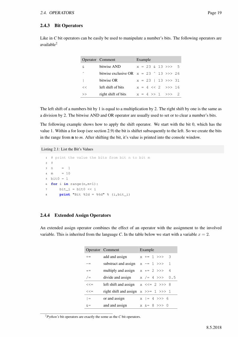
2.4.3 Bit Operators
Like in C bit operators can be easily be used to manipulate a number’s bits. The following operators areavailable2
Operator Comment Example
& bitwise AND x = 23 & 13 >>> 5
ˆ bitwise exclusive OR x = 23 ˆ 13 >>> 26
| bitwise OR x = 23 | 13 >>> 31
<< left shift of bits x = 4 << 2 >>> 16
>> right shift of bits x = 4 >> 1 >>> 2
The left shift of a numbers bit by 1 is equal to a multiplication by 2. The right shift by one is the same asa division by 2. The bitwise AND and OR operator are usually used to set or to clear a number’s bits.
The following example shows how to apply the shift operator. We start with the bit 0, which has thevalue 1. Within a for loop (see section 2.9) the bit is shiftet subsequently to the left. So we create the bitsin the range from n to m. After shifting the bit, it’s value is printed into the console window.
Listing 2.1: List the Bit’s Values
1 # print the value the bits from bit n to bit m
2 #
3 n = 1
4 m = 10
5 bit0 = 1
6 for i in range(n,m+1):
7 bit_i = bit0 << i
8 print "Bit %2d = %6d" % (i,bit_i)
2.4.4 Extended Assign Operators
An extended assign operator combines the effect of an operator with the assignment to the involvedvariable. This is inherited from the language C. In the table below we start with a variable x = 2.
Operator Comment Example
+= add and assign x += 1 >>> 3
-= substract and assign x -= 1 >>> 1
*= multiply and assign x *= 2 >>> 4
/= divide and assign x /= 4 >>> 0.5
<<= left shift and assign x <<= 2 >>> 8
<<= right shift and assign x >>= 1 >>> 1
|= or and assign x |= 4 >>> 6
&= and and assign x &= 8 >>> 0
2Python’s bit operators are exactly the some as the C bit operators.
8.5.2018

Page 20 Analysis of Structures - SS 15
2.4.5 Manipulating Bits and Hexadecimal Numbering System
If we want to manipulate a number’s bits it is obvious more clearly to use the hexadecimal representationof a number as using the elsewhere usual decimal representation. Hexadecimal numbers starts with theliteral 0x3 and uses the digits 0-9 and A-F. F is with 15 the largest digit of the hexadecimal numberingsystem. The hexadecimal numbering system has the advantage, that it packs 4 bits of a number into onehexadecimal digit. So a byte can be represented by 2 hexadecimal digits. If we now be able to translate ahexadecimal digit into a binary number, then we can see even the bits in the largest number without anycalculation.
In the following example we want to analyze the arbitrary number 27563. The bits are obviously veryhidden using the decimal representation. To get a hexadecimal representation we can simple print thenumber using the X formating. We can see that we obviously use two bytes for this number, because wieget 4 digits (6BAB). Furthermore we can see, that the leading bit is not set, because the largest digit is 6and the highest bit in a digit has the value 8.
1 >>> a = 27563
2 >>> "%X" %a
3 ’6BAB’
4 >>>
The binary number representation is easily available from the hexadecimal representation, if we knowthe binary representation of the hexadecimal digits4.
616 = 610 = 4 + 2 = 01102
A16 = 1010 = 8 + 2+ = 10102
B16 = 1110 = 8 + 2 + 1 = 10112
So we get assembling the binary digits of 6BAB the following bit sequence.
2756310 = 6BAB16 = 0110|1011|1010|10112 (2.2)
If we now want to set the highest bit of the discussed number, we can use the bitwise OR operator | (seesection 2.4.4). A number with only the highest bit set we can obtain by shifting the first bit to the desiredposition within the 2 bytes, i.e. we shift the bit 15 times. Now we can see that we get a hexadecimalnumber with only the highest digit non vanishing. Within the digit of 8 the forth bit is set, which is thehighest of a have byte5.
1 >>> b = 1
2 >>> b = b<<15
3 >>> b
4 32768
5 >>> "%X" % b
6 ’8000’
If we now want to set the highest bit of our original number 27563, we simple can overlay it with the lastnumber 8000.
3A binary number starts with the literal 0b and uses the digits 0 and 1, like 0b1000 = 810.4The index of the example’s numbers represent the base of the numbering system.5A half byte is also called nibble.
E. Baeck

2.4. OPERATORS Page 21
1 >>> a = 27563
2 >>> b = a | (1<<15)
3 >>> b
4 60331
5 >>> "%X" % b
6 ’EBAB’
After having set the highest bit, we see that the decimal number has changed totally. However thehexadecimal number only changes in the first digit. Instead of 6 we have now E. And E is representedbinary with
E16 = 1410 = 8 + 4 + 2 = 11102
so we get
6033110 = EBAB16 = 1110|1011|1010|10112 (2.3)
Comparing the binary result with the binary result of equation 2.2 we see that obiously only the first bitis set as wanted.
How we can now clear a bit of a number? Clearing a bit of a number uses two steps. First we have tocreate the inverse of the filtering number, having set only the desired bit. And within a second step weuse the AND operator & to overlay bitwise the inverse of the filtering number and the number, whose bitshould be cleared. In our example we want to clear the highest bit of the first byte. The filtering numberwe get shifting the 1st bit 7 times.
1 >>> a = 27563
2 >>> b = a & (˜(1<<7))
3 >>> b
4 27435
5 >>> "%X" % b
6 ’6B2B’
We also notice, that the decimal representation has changed widely after the clearing of the bit on thecontrary to the hexadecimal.
2743510 = EB2B16 = 1110|1011|0010|10112 (2.4)
2.4.6 Comparison Operators
Boolean operators are used to branch and to make decisions. The comparing operators are identical tothe C comparing operators.6
Operator Comment Example
< less than x = 23 < 13 >>> False
<= less equal x = 23 <= 23 >>> True
> greater x = 23 > 13 >>> True
>= left shift of bits x = 23 >= 23 >>> True
== equal x = 23 == 23 >>> True
!= non equal x = 23 != 23 >>> False
<> not equal x = 23 <> 13 >>> False
6There are two identical non equal operators available. ! = is C like, and <> is Basic like, the later one is obsolete andtaken from Phyton 3.
8.5.2018

Page 22 Analysis of Structures - SS 15
The result of a boolean expression like above are the boolean values False or True. To combinecomparing expressions the following logical operators can be used.7
Operator Comment Example
and logical and x = 1 < 2 and 2 < 3 >>> True
or logical or x = 1 < 2 or 2 > 3 >>> True
not logical not x = not (1 < 2) >>> False
The following table shows the truth values of the && and the || operator.
Truth tabel of the && operator
a b a && b
true true true
true false false
false true false
false false false
Truth tabel of the || operator
a b a || b
true true true
true false true
false true true
false false false
2.4.7 Membership Operators
With the membership operators you can check whether a value or an object is part of sequence of objects.
Operator Comment Example
in is member x = 2 in (1,2,3) >>> True
not in is not a member x = 2 not in (1,2,3) >>> False
2.4.8 Identity Operators
With the identity operators you can check the identity of two objects.
Operator Comment Example
is is identical x = (1,2) >>> y = x >>> x is y >>> True
is not is not identical x = (1,2) >>> y = x >>> x is not y >>> False
7To make expressions clear parenthesis should be used. A term within a parenthesis is evaluated first and it’s result then isused in further evaluations outside the parenthesis. With parenthesis the order of the evaluation can be set.
E. Baeck
2.5. PRINT AND OUTPUT FORMATS Page 23
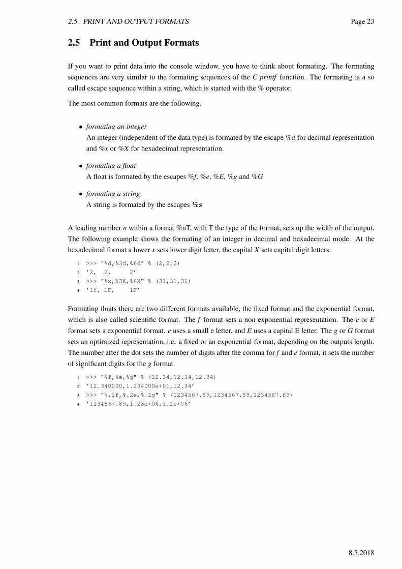
2.5 Print and Output Formats
If you want to print data into the console window, you have to think about formating. The formatingsequences are very similar to the formating sequences of the C printf function. The formating is a socalled escape sequence within a string, which is started with the % operator.
The most common formats are the following.
• formating an integerAn integer (independent of the data type) is formated by the escape %d for decimal representationand %x or %X for hexadecimal representation.
• formating a floatA float is formated by the escapes %f, %e, %E, %g and %G
• formating a stringA string is formated by the escapes %s
A leading number n within a format %nT, with T the type of the format, sets up the width of the output.The following example shows the formating of an integer in decimal and hexadecimal mode. At thehexadecimal format a lower x sets lower digit letter, the capital X sets capital digit letters.
1 >>> "%d,%3d,%6d" % (2,2,2)
2 ’2, 2, 2’
3 >>> "%x,%3X,%6X" % (31,31,31)
4 ’1f, 1F, 1F’
Formating floats there are two different formats available, the fixed format and the exponential format,which is also called scientific format. The f format sets a non exponential representation. The e or Eformat sets a exponential format. e uses a small e letter, and E uses a capital E letter. The g or G formatsets an optimized representation, i.e. a fixed or an exponential format, depending on the outputs length.The number after the dot sets the number of digits after the comma for f and e format, it sets the numberof significant digits for the g format.
1 >>> "%f,%e,%g" % (12.34,12.34,12.34)
2 ’12.340000,1.234000e+01,12.34’
3 >>> "%.2f,%.2e,%.2g" % (1234567.89,1234567.89,1234567.89)
4 ’1234567.89,1.23e+06,1.2e+06’
8.5.2018

Page 24 Analysis of Structures - SS 15
2.6 Basic Data Types
Recording to the available data types, Python is very different comparing it with common languages likeC, Fortran and Basic. Most of the languages offers the programmer data types, which are one by onerelated to the underlaying hardware.
So for example Fortran and C offer 2 and 4 byte integers on 32 bit operating systems by default8 On a64 bit operating platform a long integer of 8 bytes will be available. On the other hand there are 4 and 8byte floats available.
Python however offers on 32 bit platforms a normal integer of 4 bytes, which is directly related to thehardware, for example 11234, and furthermore a so called long integer, for example 1234L, which ishandled by the Python software. The long integer, which is marked by a succeeding L, is only restrictedby the computers memory, that means that a really incredible number of digits can be considered. Laterwe will calculate the factorial of a incredible high number.
Furthermore Python as already mentioned offers only one float data type with 8 bytes. The standardized4 byte float is not supported, for example 1.23 or 1.23e+2.
Python also supports a complex arithmetic with an complex data type, consisting of two floats for realand imaginary part of the complex number. The complex unit in Python is called j. Therefor the complexnumber 1 + 4i will be represented in Python with 1 + 4j.
The last data type used in Python is a string consisting of one or more characters.
The data type of a variable can be determined using the build in function type, as shown in the followingexample. Within a first step different variables were created by a simple assignment. The content of thevariable determines the type of the variable, no explicit declaration is needed or available, like in C. Afterhaving created the variables the type of the variables will be determined by subsequent type calls.
To check the data type within a program the following tests can be made.
1. if type(d).__name__ == ’int’
You can check the type with the types __name__ member.
2. if type(d) == int
... or you can check the type with the type class name (discussed later).
1 >>> a = 2
2 >>> b = 3L
3 >>> c = 4.5
4 >>> d = 6 + 7j
5 >>> e = "Hello World"
6 >>> type (a)
7 <type ’int’>
8 >>> type (b)
9 <type ’long’>
10 >>> type (c)
11 <type ’float’>
12 >>> type(d)
13 <type ’complex’>
8That means without applying provider depended tricks.
E. Baeck
2.7. CODE BLOCKS Page 25
14 >>> type(e)
15 <type ’str’>
You see, ’int’ is integer, ’long’ is long integer, ’float’ is float, ’complex’ is complex and’str’ is string data type.
Furthermore there are some sequences in Python available, which combines the mentioned data types ina more or less sophisticated mode. More about that later.
2.7 Code Blocks
One very imported feature of Python is, that code blocks are bracketed by an unique indent. The mostprogramming languages uses there specific code parenthesis. There is one opening parenthesis whichstarts the code block and there is one closing parenthesis, which closes the code block.
The following example shows a code block in C.
1 if (a > b)
2 {
3 c = a + b
4 d = a - b
5 ... Further Lines of C-Code ...
6 }
The following example shows a code block in Fortran77.
1 if (a .gt. b) then
2 c = a + b
3 d = a - b
4 ... Further Lines of Fortran-Code ...
5 endif
Compared with this in Python the code block is bracketed by indent as follows.
1 if a > b:
2 c = a + b
3 d = a - b
4 ... Further Lines of Python-Code ...
5 a = b
One statement which uses a code block, in this case an if statement, is closed by a colon. After the colonan unique indent for the lines of the code block must be used. If not, it will be a syntax error. The codeblock is closed, if the last line of the code block is the last line of the whole code, or is closed by a lineof code which is indented like the opening statement. In our example the assignment a=b has the sameindent as the if statement and so this line will be the first line of code outside our code block.
8.5.2018

Page 26 Analysis of Structures - SS 15
2.8 Globales
In Python a variable will be created, if an assignment is done. If so, it is impossible to access a variable,which is introduced elsewhere, i.e. a global variable. If we now want to access such a variable, we haveto declare it inside our local function as a global variable. If we do this, the Python interpreter is lookingfor a variable with such a name inside the name space of the calling function.
Example 2.2 shows how to access a global variable and which effect we have, if the value is changedinside the called function.
Listing 2.2: Testing Global Variables
1 # usage of global
2
3 def doSomething(a):
4 global b
5
6 print "doSomething...: a = %d, b = %d" % (a,b)
7
8 a = 10 # local variable
9 b = 20 # global variable
10 c = 30 # local variable
11 print "doSomething...: a = %d, b = %d, c = %d" % (a,b,c)
12
13 a = 1
14 b = 2
15 c = 3
16 print "before calling: a = %d, b = %d, c = %d" % (a,b,c)
17 doSomething(a)
18 print "after calling.: a = %d, b = %d, c = %d" % (a,b,c)
Listing 2.3: Output from the Testing Example
1 before calling: a = 1, b = 2, c = 3
2 doSomething...: a = 1, b = 2
3 doSomething...: a = 10, b = 20, c = 30
4 after calling.: a = 1, b = 20, c = 3
In the output listing from our little testing example 2.2 we see, that the value of the global variable bis overwritten by the function call, the value of the local variable a only is changed inside the function.After the function call we see, that the variable a remains untouched by the function call.
E. Baeck

2.9. LOOP FOR REPETITIONS Page 27
2.9 Loop for Repetitions
Like all programming languages, which make sense, Python also has some implementations of repe-titions, of loops. Like in C an explicit loop is available - the for loop - as well as an implicit loop isavailable - the while loop.
The for loop is controlled by an iterated set. One very common variant is the for loop, which is controlledby an iteration counter. The iteration counter will be configured by a range object. The range object has3 parameters9. The first parameter sets the start value of the iteration counter, the second parameter setsup the iteration value, which will be the first value that is not performed. The third parameter sets up theincrement.
2.9.1 The Factorial
The following typical example for the usage of an iterative for loop implements the calculation of thefactorial.
n! =
n∏i=1
i (2.5)
The implementation of the factorial is given below. Note the importance of the indent, see section 2.7.
1 n = 10 # factorial input
2 p = 1 # result variable must be initalized by 1
3 for i in range(2,n+1): # the counter runs from 2 up to n
4 p *= i # here we perform the product
5 print "%3d! = %10d" % (n,p) # write the result into the console
6
7 >>>... console window ...
8 10! = 3628800
The second loop type, the while loop is working implicit with a boolean expression, which controls thebreak condition. If we want to implement the factorial using the while loop we get the following code.
1 n = 10 # factorial input
2 p = 1 # result variable must be initalized by 1
3 i = 2 # the counter runs from 2 up to n
4 while i <=n: # loop with break condition
5 p *= i # perform the product
6 i += 1 # explicit incrementation
7 print "%3d! = %10d" % (n,p)
8
9 >>>... console window ...
10 10! = 3628800
9A parameter is a information unit, which is passed to the called object. If more then one parameter is passed, the parametersare separated by commas.
8.5.2018

Page 28 Analysis of Structures - SS 15
The next example shows a nested loop. Very important is the correct code block indent.
1 for i in range(0,4): # outer loop
2 for j in range(0,2): # inner loop
3 print "i:%2d, j:%2d" % (i,j) # print counter variables
4
5 >>>... console window ...
6 i: 0, j: 0
7 i: 0, j: 1
8 i: 1, j: 0
9 i: 1, j: 1
10 i: 2, j: 0
11 i: 2, j: 1
12 i: 3, j: 0
13 i: 3, j: 1
For the detailed controlling of the loops cycles two statements are available.
• continueIf the continue statement is used a cycle is immediately stopped and the next cycle is started.
• breakIf the break statement is used a cycle is immediately stopped and the loop is exited.
The next example shows an application of the continue statement. A loop is performed with the values0 · · · 4. The cycle with the counter 2 is prematurely canceld.
1 >>> for i in range(0,5):
2 ... if i == 2: continue
3 ... print "i=%d" % i
4 ...
5 i=0
6 i=1
7 i=3
8 i=4
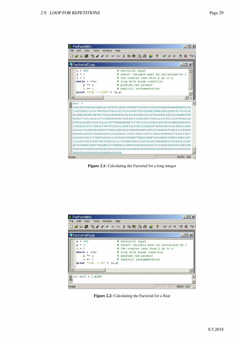
One very interesting feature of Python is the long integer arithmetic. So we can calculate incredible largefactorials. Figure 2.1 shows the code in the upper window. The console window shows the result. Anumber with a lot of digits and every digit is exact.
The next example shows the calculation of the factorial using a float. The float factorial can only beevaluated up to 170! = 7.25742e+306. In the case of 400! we will get an overflow, because theexponent exceeds the available memory in 8 bytes (see figure 2.2).
E. Baeck
2.9. LOOP FOR REPETITIONS Page 29
Figure 2.1: Calculating the Factorial for a long integer
Figure 2.2: Calculating the Factorial for a float
8.5.2018

Page 30 Analysis of Structures - SS 15
2.9.2 Floating Point Precision
The Precision-Finder is a nice little program, which analysis the relative precision of a given float format.
2.9.2.1 Description of the Application
Start
Initializing:X1 = 1.; X2 = 1.; D = 2.;
Reductionstep:X2 = X2/D;
Accumulationstep:S = X1 +X2;
S > X1yes
Resultstep:Precission = X2 * D;
no
Stop
Figure 2.3: Flowchart for a Precision Finder
As we know, the computer cannot handle an infinite numberof floating-point digits. Therefore it is important to know whomany digits are available in a floating-point format (float).Figure 2.3 shows a flow chart of an algorithm which continu-ally reduces the value of a variable. After each reduction thesum of the fixed and the reduced variable is calculated. If nowthe contribution of the reduced is vanishing, we have reachedthe total limit. Beyond this limit the contributing informationis totally expunged. To get the relative precision, i.e. relatingto one, we have to take back the last reduction, if we havereached the limit.
2.9.2.2 Exercise
Please implement the algorithm of the Precision-Finder forthe Python float format within a little script like the famousHello World example (see section 1.3).
E. Baeck
2.10. FUNCTIONS Page 31
2.10 Functions
A function is a callable type. A function starts with the def command. The parameter list succeeds thefunction name and consists of names separated by commas. The return of return values is optional. Ifmore then one return value should be given, the return values are separated by commas and the callingcode will get a tuple containing all the return values. A single return value is not returned in a tuple.
A nice example to study cases of a solution and their specific return values is discussed in section 2.11.
1 def <name> (Parameter list):
2 Code Block
3 return <Return Object list>
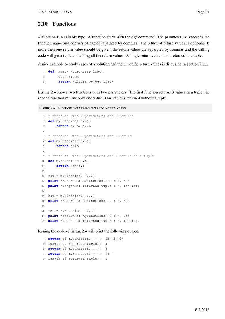
Listing 2.4 shows two functions with two parameters. The first function returns 3 values in a tuple, thesecond function returns only one value. This value is returned without a tuple.
Listing 2.4: Functions with Parameters and Return Values
1 # function with 2 parameters and 3 returns
2 def myFunction1(a,b):
3 return a, b, a**b
4
5 # function with 2 parameters and 1 return
6 def myFunction2(a,b):
7 return a**b
8
9 # function with 3 parameters and 1 return in a tuple
10 def myFunction3(a,b):
11 return (a**b,)
12
13 ret = myFunction1 (2,3)
14 print "return of myFunction1... : ", ret
15 print "length of returned tuple : ", len(ret)
16
17 ret = myFunction2 (2,3)
18 print "return of myFunction2... : ", ret
19
20 ret = myFunction3 (2,3)
21 print "return of myFunction3... : ", ret
22 print "length of returned tuple : ", len(ret)
Runing the code of listing 2.4 will print the following output.
1 return of myFunction1... : (2, 3, 8)
2 length of returned tuple : 3
3 return of myFunction2... : 8
4 return of myFunction3... : (8,)
5 length of returned tuple : 1
8.5.2018

Page 32 Analysis of Structures - SS 15
2.11 Branches for Decisions
Decisions are made by the usage of the if statement. The if statement is defined as follows.
1 if [boolean expression 1]:
2 code block 1
3 elif [boolean expression 2]:
4 code block 2
5 elif [boolean expression 3]:
6 code block 3
7
8 ...
9 else:
10 code block else
2.12 Conditional Assignments
Like in languages like C/C++ in Python there is a similar conditional assignment available.
1 <variable> = <value_1> if <boolean expression> else <value_2>
In listing 2.12 we get an i value of 3, because b is true. Otherwise we would get a zero value.
1 b = true
2 i = 3 if b else 0 # in C: i = b ? 3:0;
2.12.1 How to Solve a Quadratic Equation
The calculation of roots of a quadratic equation is a nice and simple example to show the application ofthe if statement. The quadratic equation is given by
a · x2 + b · x+ c = 0 (2.6)
If we want to solve the quadratic equation, we have to analyze the available cases. A general solutionmust handle the following cases.
• constant casea = b = c = 0
• linear casea = 0, b 6= 0
• quadratic casea 6= 0
• no solution casea = b = 0 and c 6= 0
E. Baeck

2.12. CONDITIONAL ASSIGNMENTS Page 33
2.12.1.1 A Flow-Chart
The following flow chart shows all the case, which we have to handle. The algorithm is given for a realarithmetic, i.e. no complex data types are used. The relevant source code will be developed within thenext section.
Start
a = 0 b = 0 c = 0infinit
solutionsStop
no solution Stopx = − cb Stopd = b2 − 4 · a · c
d < 0 x1,2 = −b±i√−d
2·a Stop
x1,2 = −b±√d
2·a Stop
yes yes yes
nonono
yes
no
2.12.1.2 The Implementation
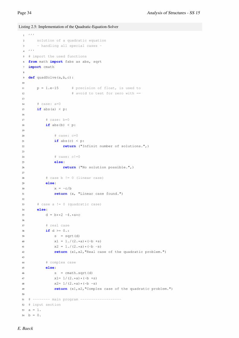
The implementation uses a real as well a complex arithmetic importing the module math and cmath. Thesolver of the quadratic equation is implemented in a function called QuadSolve. The function analyzesthe different cases and returns in the constant case only a comment, in the linear case the solution valueand a comment. In the quadratic case 2 values and a comment were returned. All return values arepacked into a tuple. The case can be identified form the calling program using the function len, whichreturns the number of items of a tuple. To branch in the real respectively the complex quadratic case, wehave to check the type of the returned result values using the Python function type. This we see in line75. If the type is complex, we have to extract the real and the imaginary part of the number, to print itusing the print statement.
From line 44 on, we can see that using the complex square-root function cmath.sqrt automatically weget a complex result. So it’s possible too, to return in any quadratic case a complex results. If so, wedon’t need to branch.
To avoid the testing for zero, which would produce numerical problems in principle, we set the relativeprecision to 10−15. An absolute value less then this relative precision is treated as zero value. Here weapply the function fabs from the math package introducing the alias abs. Here we should know, thatPython provides a buildin function abs, which then will be overlayed by the fabs, so that the buildin isvisible no more.
8.5.2018
Page 34 Analysis of Structures - SS 15
Listing 2.5: Implementation of the Quadratic-Equation-Solver
1 ’’’
2 solution of a quadratic equation
3 - handling all special cases -
4 ’’’
5 # import the used functions
6 from math import fabs as abs, sqrt
7 import cmath
8
9 def quadSolve(a,b,c):
10
11 p = 1.e-15 # precision of float, is used to
12 # avoid to test for zero with ==
13
14 # case: a=0
15 if abs(a) < p:
16
17 # case: b=0
18 if abs(b) < p:
19
20 # case: c=0
21 if abs(c) < p:
22 return ("Infinit number of solutions.",)
23
24 # case: c!=0
25 else:
26 return ("No solution possible.",)
27
28 # case b != 0 (linear case)
29 else:
30 x = -c/b
31 return (x, "Linear case found.")
32
33 # case a != 0 (quadratic case)
34 else:
35 d = b**2 -4.*a*c
36
37 # real case
38 if d >= 0.:
39 s = sqrt(d)
40 x1 = 1./(2.*a)*(-b +s)
41 x2 = 1./(2.*a)*(-b -s)
42 return (x1,x2,"Real case of the quadratic problem.")
43
44 # complex case
45 else:
46 s = cmath.sqrt(d)
47 x1= 1/(2.*a)*(-b +s)
48 x2= 1/(2.*a)*(-b -s)
49 return (x1,x2,"Complex case of the quadratic problem.")
50
51 # -------- main program -------------------
52 # input section
53 a = 1.
54 b = 0.
E. Baeck

2.13. FUNCTION EXAMPLES Page 35
55 c = 4.
56
57 # call of QaudSolve function
58 result = quadSolve(a,b,c)
59
60 # check the result tuple, to select the found case
61 values = len(result)
62 print "%d values found in return" % values
63
64 # format the found result case
65 # no or infinit solution(s)
66 if values == 1:
67 print result[0]
68
69 # linear case
70 elif values == 2:
71 print "x = %f, info: %s" % result # (result[0],result[1])
72
73 # quadratic case
74 elif values == 3:
75 if type(result[0]) == complex:
76 print "x1 = %f+(%fi), x2= %f+(%fi), info: %s" \
77 % (result[0].real,result[0].imag,
78 result[1].real,result[1].imag,
79 result[2])
80 else:
81 print "x1 = %f, x2 = %f, info: %s" % result
2.13 Function Examples
In this section we will discuss a new abs function and the Newton algorithm using a function as parameter.
2.13.1 An Abs-Function with Type-Checking
The following code shows a special version of the abs function. The data type is checked first. Only int,long or float type are senseful supported. We check the type with the type function. The type functionreturns a type object. Within the function we check the object member __name__. If the type is notsupported, a error string is returned. If the type is supported, the return value is return. The callingprogram checks the return values type using the object name (int, long and float).
Listing 2.6: Abs Function with Type Checking
1 # declaring our version of an abs function
2 def myAbs(x):
3
4 # process only sensful data types
5 # here we use the type class member __name__
6 # to check the data type
7 t = type(x).__name__
8 if t != ’int’ and t != ’long’ and t != ’float’:
9 return "Error: Type ’%s’ is not allowed." %t
10
8.5.2018

Page 36 Analysis of Structures - SS 15
11 # if data type ok change sign if necessary
12 if x < 0.: return -x
13 return x
14
15 # input section
16 y = -4 # test 1
17 # y = "hello" # test 2
18
19 # function call
20 z = myAbs(y)
21
22 # get return type
23 t = type(z)
24 if t == str: # second version to check the type
25 print z # print error message
26 else:
27 print "Absolute Value of %f = %f" % (y,z) # print result
2.13.2 The Newton-Algorithm
Figure 2.4: Scheme of the Newton Algorithm
The following example shows, how to pass a function asa functions parameter. Within the Newton’s algorithma root of an equation should be calculated. So we haveto specify the function of interest. This function can beconsidered as an input parameter. This function nameis passed to the derivative calculator and to the newtonmain routine. Further we see, that it’s recommended touse standard parameter, to configure the algorithm. Weintroduce the precision parameter e, which sets up thethreshold for a zero compare. Further we need the stepwidth to calculate the derivative of the function of ourinterest.
The derivative - it’s called fs in the code - is calculated numerical as follows.
f ′(x) =df
dx≈
(f(x+
h
2)− f(x− h
2)
)/h
(2.7)
The Newton scheme can be described as follows.
xi+1 = xi −f(x)
f ′(x)(2.8)
E. Baeck
2.13. FUNCTION EXAMPLES Page 37
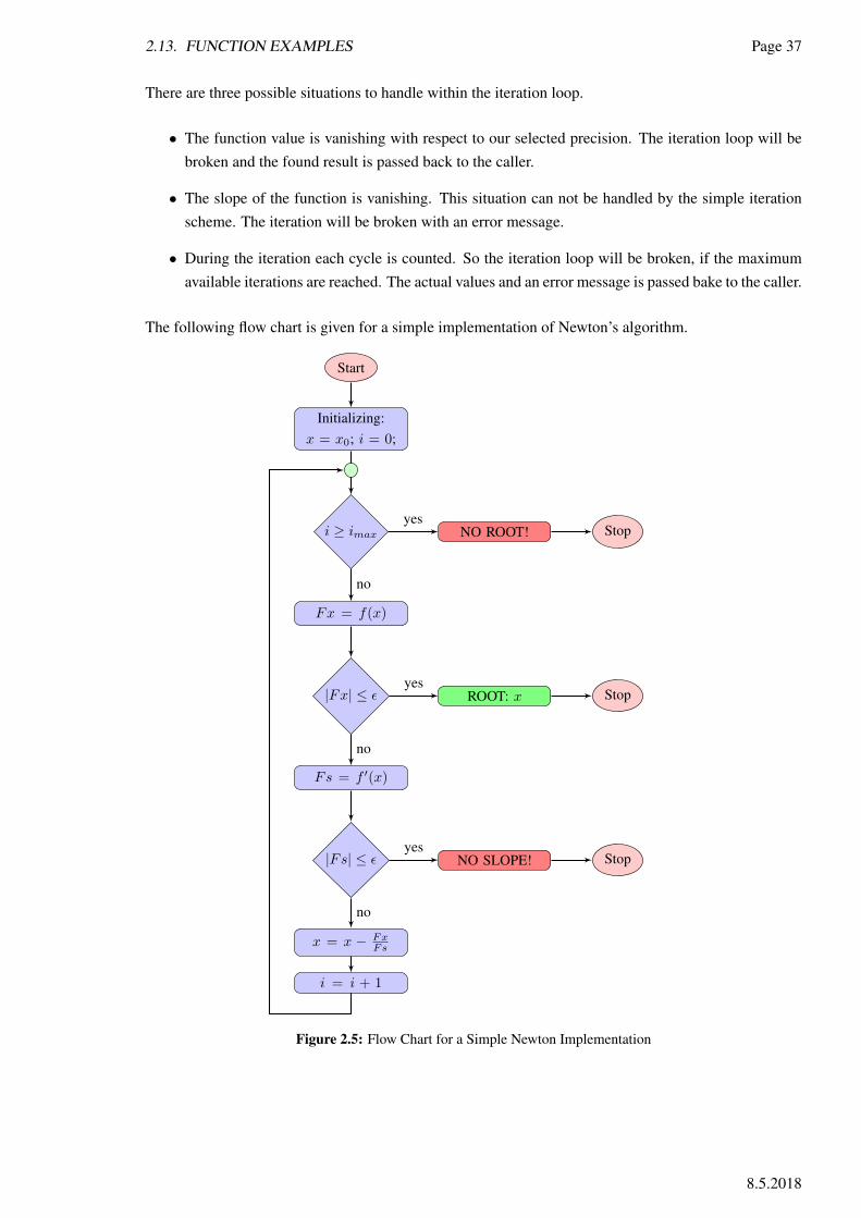
There are three possible situations to handle within the iteration loop.
• The function value is vanishing with respect to our selected precision. The iteration loop will bebroken and the found result is passed back to the caller.
• The slope of the function is vanishing. This situation can not be handled by the simple iterationscheme. The iteration will be broken with an error message.
• During the iteration each cycle is counted. So the iteration loop will be broken, if the maximumavailable iterations are reached. The actual values and an error message is passed bake to the caller.
The following flow chart is given for a simple implementation of Newton’s algorithm.
Start
Initializing:x = x0; i = 0;
i ≥ imax NO ROOT!yes
Stop
Fx = f(x)
no
|Fx| ≤ ε ROOT: xyes
Stop
Fs = f ′(x)
no
|Fs| ≤ ε NO SLOPE!yes
Stop
x = x − FxFs
no
i = i + 1
Figure 2.5: Flow Chart for a Simple Newton Implementation
8.5.2018

Page 38 Analysis of Structures - SS 15
The code consists of the following functions.
• myF, the function of our interest.
• fs, the function which calculates the slope of a given function numerically.
• newton, implements the newton scheme.
Listing 2.7: Implementation of Newton’s-Alogrithm
1 from math import fabs as abs # import the fabs as abs
2
3 # implementation of the function of interest
4 def myF(x):
5 return x**2 +1.
6
7 # calculating the derivative
8 def fs(f,x,h=1.e-6):
9 h = float(h)
10 x = float(x)
11 return (f(x+0.5*h) - f(x-0.5*h))/h
12
13 # implementation of a newton algorithm
14 def newton(f,x0,e=1.e-10,h=1.e-6,imax=100):
15
16 error = None # initialize the error code with None
17
18 h = float(h) # we need some floats
19 e = float(e)
20 x1= float(x0) # x to interate
21
22 i = 1 # iteration counter
23 while True:
24
25 f0 = f(x1) # function’s value
26 if abs(f0) < e:
27 break
28
29 # calculating the derivative
30 f1 = fs(f,x1,h)
31 if abs(f1) < e:
32 error = "*** Error: vanishing derivate!"
33 break
34
35 # available iterations exceeded
36 if i >= imax:
37 error = "*** Error: no root found!"
38 break
39
40 # calculating the values for next iteration
41 x1 -= f0/f1
42
43 # increment the iteration counter
44 i+=1
45
46 # return the actual position, the function value
E. Baeck

2.14. DATA SEQUENCES Page 39
47 # and the functions slope, the number of performed
48 # iterations and the error code.
49 return (x1,f0,f1,i,error)
50
51 # the function newton is called with standard parameters
52 # we pass the function of interest and a supposed start
53 # position
54 res = newton(myF,4.)
55
56 # the returned tuple is printed into the console window
57 print res
2.14 Data Sequences
In Python there are some sequential data types available.
• Strings, a list of characters.
• Tuples are fixed sequences, which are only extensible. The advantage of tuples is the performance.
• Lists are changeable sequences but with lower performance.
2.14.1 Working with Tuples
The following example shows the creation of a tuple. An empty tuple is declared. We extend the tuplewith a one element tuple - note the comma. The second extension extends the tuple with a two elementtuple.
1 >>> t = () # initialize the tuple
2 >>> t
3 ()
4 >>> t += (1,) # append the tuple with a number
5 >>> t
6 (1,)
7 >>> t += (2,3) # append at tuple with a second tuple
8 >>> t
9 (1, 2, 3)
10 >>> t[0] # calling the tuple’s first element
11 1
12 >>> t[2] # calling the tuple’s third element
13 3
14 >>> t[3] # an error occur, if the index goes out of range
15 Traceback (most recent call last):
16 File "<interactive input>", line 1, in <module>
17 IndexError: tuple index out of range
18 >>> len(t) # the number of elements is given by the len function
19 3
8.5.2018

Page 40 Analysis of Structures - SS 15
Note, that tuples are input data for complex string formatings.
1 >>> "x1 = %8.2f, x2 = %8.3f" % (12.3456,12.3456)
2 ’x1 = 12.35, x2 = 12.346’
With the function tuple() a tuple can be created from an iterable object like string or list.
1 >>> T =tuple([1.,2.])
2 >>> T
3 (1.0, 2.0)
4 >>> L = list(T)
5 >>> L
6 [1.0, 2.0]
7 >>> T = tuple("Hello World")
8 >>> T
9 (’H’, ’e’, ’l’, ’l’, ’o’, ’ ’, ’W’, ’o’, ’r’, ’l’, ’d’)
Note, that the data of a list can be converted into a tuple using the function tuple() and reverse into alist using the function list().
2.14.2 Working with Lists
Lists are more flexible as tuples. Creating and extending lists can be coded like in the case of tuples.The only difference is, that lists uses in their declaration the [..] parenthesis. So using lists the codeexample of the section 2.14.1 can be coded like follows.
1 >>> L = {] # initialize the list
2 >>> L
3 []
4 >>> L += [1,] # append the list with a number
5 >>> L
6 [1,]
7 >>> L += [2,3] # append at list with a second list
8 >>> L
9 [1, 2, 3]
10 >>> L[0] # calling the lists first element
11 1
12 >>> L[2] # calling the list’s third element
13 3
14 >>> len(L) # the number of elements is given by the len function
15 3
You can read somewhere, that tuples are much more faster than lists. This is surely not valid for everyproblem. So it’s recommended to check the performance explicitly before you decide to use tuples orlists.
The list object offers a wide set of methods. Some of them are discussed in the following table.
E. Baeck
2.14. DATA SEQUENCES Page 41
Methode Comment Example
append(i) Append an item to the list. Same as += operator. L.append(3)
count(x) Counts the value x in the list. L.count(1.2)
extend(s) Append a list to the list. Same as += operator. L.extend(t)
index(x) Evaluates the lowest index of the value x in the list. L.index(1.2)
insert(i,x) Inserts the object x before the item i. L.insert(2,1.2)
pop() Returns the last item and deletes it from the list. L.pop()
remove(x) Removes the first item with the value x. L.remove(1.2)
reverse() Invert the order of the items of a list. L.reverse()
sort() Sort the items of list in ascending order. L.sort(t)
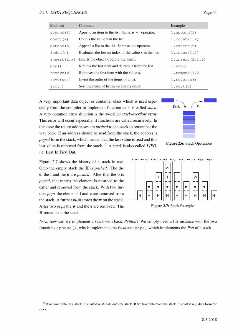
Figure 2.6: Stack Operations
A very important data object or container class which is used espe-cially from the compiler to implement function calls is called stack.A very common error situation is the so-called stack-overflow error.This error will occur especially, if functions are called recursively. Inthis case the return addresses are pushed to the stack to remember theway back. If an address should be read from the stack, the address ispoped form the stack, which means, that the last value is read and thislast value is removed from the stack.10 A stack is also called LIFO,i.e. Last In First Out.
Figure 2.7: Stack Example
Figure 2.7 shows the history of a stack in use.Onto the empty stack the H is pushed. The thee, the l and the o are pushed. After that the o ispoped, that means the element is returned to thecaller and removed from the stack. With two fur-ther pops the elements l and e are removed fromthe stack. A further push stores the w on the stack.After two pops the w and the e are removed. TheH remains on the stack
Now, how can we implement a stack with basic Python? We simply need a list instance with the twofunctions append(), which implements the Push and pop() which implements the Pop of a stack.
10If we save data on a stack, it’s called push data onto the stack. If we take data from the stack, it’s called pop data from thestack.
8.5.2018
Page 42 Analysis of Structures - SS 15
2.14.3 Working with Dictionaries
A dictionary is a powerful and very general container, it’s also called map, because a key value is mappedonto the pointer of the stored item. In Python an instance pointers is stored in a dictionary using anarbitrary key strings. So a dictionary is like a list container with a more general access. Because thedictionary commonly hashes the key information onto some smaller index lists, the dictionary commonlyhas a better performance as a linked list container. The dictionary therefore is used in the abaqus classlibrary (we will discuss it later) to store named instances.
A dictionary can be created like a list using curled parenthesis. Each key-value pair is separated by acomma. The key is separated from the value by a colon.
1 >>> myDict = {’first item’:1, ’second item’:2}
2 >>> print myDict[’second item’]
3 2
4 >>> beatles = {}
5 >>> beatles[’drums’] = ’Ringo’
6 >>> beatles[’bass’] = ’Paul’
7 >>> beatles[’vocal’] = ’John, Paul, George, Ringo’
8 >>> beatles[’guitar’] = ’George, John’
9 >>> print beatles
10 {’guitar’: ’George, John’, ’vocal’: ’John, Paul, George, Ringo’, ’bass’: ’Paul’,
11 ’drums’: ’Ringo’}
2.15 Error Handling with Exceptions
There are (at least) two distinguishable kinds of errors: syntax errors and exceptions.11
2.15.1 Syntax Errors
Syntax errors, also known as parsing errors, are perhaps the most common kind of complaint you getwhile you are still learning Python.
1 >>> while True print ’Hello world’
2 File "<stdin>", line 1, in ?
3 while True print ’Hello world’
4 ˆ
5 SyntaxError: invalid syntax
The parser repeats the offending line and displays a little arrow pointing at the earliest point in the linewhere the error was detected. The error is caused by (or at least detected at) the token preceding thearrow: in the example, the error is detected at the keyword print, since a colon (’:’) is missing before it.File name and line number are printed so you know where to look in case the input came from a script.
11Parts of this section are taken from the Python 2.7 manual.
E. Baeck
2.15. ERROR HANDLING WITH EXCEPTIONS Page 43
2.15.2 Exceptions
Even if a statement or expression is syntactically correct, it may cause an error when an attempt is madeto execute it. Errors detected during execution are called exceptions and are not unconditionally fatal. Wewill see how to handle them in the next section. Most exceptions are not handled by programs, however,and result in error messages as shown below.
1 >>> 10 * (1/0)
2 Traceback (most recent call last):
3 File "<stdin>", line 1, in ?
4 ZeroDivisionError: integer division or modulo by zero
5 >>> 4 + spam*3
6 Traceback (most recent call last):
7 File "<stdin>", line 1, in ?
8 NameError: name ’spam’ is not defined
9 >>> ’2’ + 2
10 Traceback (most recent call last):
11 File "<stdin>", line 1, in ?
12 TypeError: cannot concatenate ’str’ and ’int’ objects
The last line of the error message indicates what happened. Exceptions come in different types, andthe type is printed as part of the message: the types in the example are ZeroDivisionError,NameError and TypeError. The string printed as the exception type is the name of the built-inexception that occurred. This is true for all built-in exceptions, but need not be true for user-definedexceptions (although it is a useful convention). Standard exception names are built-in identifiers (notreserved keywords).
The rest of the line provides detail based on the type of exception and what caused it.
The preceding part of the error message shows the context where the exception happened, in the form ofa stack traceback. In general it contains a stack traceback listing source lines; however, it will not displaylines read from standard input.
2.15.3 Handling Exceptions
It is possible to write programs that handle selected exceptions. Look at the following example, whichasks the user for input until a valid integer has been entered, but allows the user to interrupt the program(using Control-C or whatever the operating system supports); note that a user-generated interruption issignalled by raising the KeyboardInterrupt exception.
1 >>> while True:
2 ... try:
3 ... x = int(raw_input("Please enter a number: "))
4 ... break
5 ... except ValueError:
6 ... print "Oops! That was no valid number. Try again..."
7 ...
The try statement works as follows.
• First, the try clause (the statement(s) between the try and except keywords) is executed.
• If no exception occurs, the except clause is skipped and execution of the try is finished.
8.5.2018
Page 44 Analysis of Structures - SS 15
• If an exception occurs during execution of the try clause, the rest of the clause is skipped. Thenif its type matches the exception named after the except keyword, the except clause is executed,and then execution continues after the try.
• If an exception occurs which does not match the exception named in the except clause, it is passedon to outer try; if no handler is found, it is an unhandled exception and execution stops with amessage as shown above.
A try may have more than one except clause, to specify handlers for different exceptions. At mostone handler will be executed. Handlers only handle exceptions that occur in the corresponding try
clause, not in other handlers of the same try. An except clause may name multiple exceptions as aparenthesized tuple.
1 ... except (RuntimeError, TypeError, NameError):
2 ... pass
In the next example we open a file with the name ’input.dat’. We read one line and strip the leading andtrailing blanks. The result will then be converted to an integer. We know that this is not possible in everycase, so we want to handle possible errors by our error handler.
1 try:
2 f = open(’input.dat’) # let’s open then input file,
3 s = f.readline() # read the first line and
4 i = int(s.strip()) # strip the white spaces
5 except IOError as e: # catch the io-errors
6 print "I/O error(%d): %s" % (e.errno, e.strerror)
7 except ValueError: # catch conversion errors
8 print "Could not convert data to an integer."
9 except: # catch the rest
10 print "Unknown error!"
2.15.4 Raise Exceptions
If we want to avoid runtime errors, we have to check our data base. In an classical approach, we have tocheck the data, and break each activity jumping back to the origin of our call. Sometimes especial if thecalling hierarchy is extensive, it becomes an evil and tedious work to do this. On the other hand in mostmodern languages we can use exception handlers to do this work for us. The only thing we have to dois, to raise our own exception and check for it within an except clause.
The first listing 2.8 we call our square root function with a negative value.
Listing 2.8: Our Unsave mySqrt-Function
1 import math
2
3 def mySqrt(x):
4 return math.sqrt(x)
5
6 print mySqrt(-2)
The program crashes with the following output.
1 Traceback (most recent call last):
E. Baeck
2.16. RANDOM NUMBERS Page 45
2 File "C:\Python27\Lib\site-packages\Pythonwin\pywin\framework\scriptutils.py",
3 line 326, in RunScript
4 exec codeObject in __main__.__dict__
5 File "C:\UniDue\CM\Cm-AoS\AOS-BookOfExamples\Py\Code\ExceptionEx01.py", line 7,
6 in <module>
7 print Sqrt(-2)
8 File "C:\UniDue\CM\Cm-AoS\AOS-BookOfExamples\Py\Code\ExceptionEx01.py", line 4,
9 in mySqrt
10 return math.sqrt(x)
11 ValueError: math domain error
We see that obviously the function sqrt is not able to handle negative numbers.
In the next example we check the root’s value and raise an exception to break the function. This exceptionitself is caught by the main program with an try clause.
Listing 2.9: mySqrt-Function with Checking
1 import math
2
3 def mySqrt(x):
4 if x < 0.:
5 raise Exception("error: negative input value %e!" % x)
6 return math.sqrt(x)
7
8 try:
9 print mySqrt(-2)
10 except Exception as e:
11 print e
In listing 2.9 we see, that if negative values are passed, the function will raise an exception. Using theException class we send a string information, which can be caught within the except clause. Theoutput of this version is given below.
1 error: negative input value -2.000000e+00!
We see, that the concept of an exception handling is a powerful feature to implement error checking.
2.16 Random Numbers
Because a computer is system, which works systematically reproducible, a computer will not be able tocreate real random numbers. If we start a program twice with exact the same input values, the result alsowill be the same. But with a little trick, we can produce so called pseudo random numbers. If we usethe time as input for the initialization of our random number generator, we will be sure, that it will beextremely improbable, to get twice the same random number set.
So every programing language has it’s own random number generator. Python offers us a build-in pack-age, which is called random. Like in C the random number generator is to initialize with a functionseed(). This function uses the computer time information to make varying starting conditions.
The following example will discuss two features of the Python library.
• How can we use the random package to create random numbers or to create a random order oflists, i.e. shuffle the list’s data.
8.5.2018
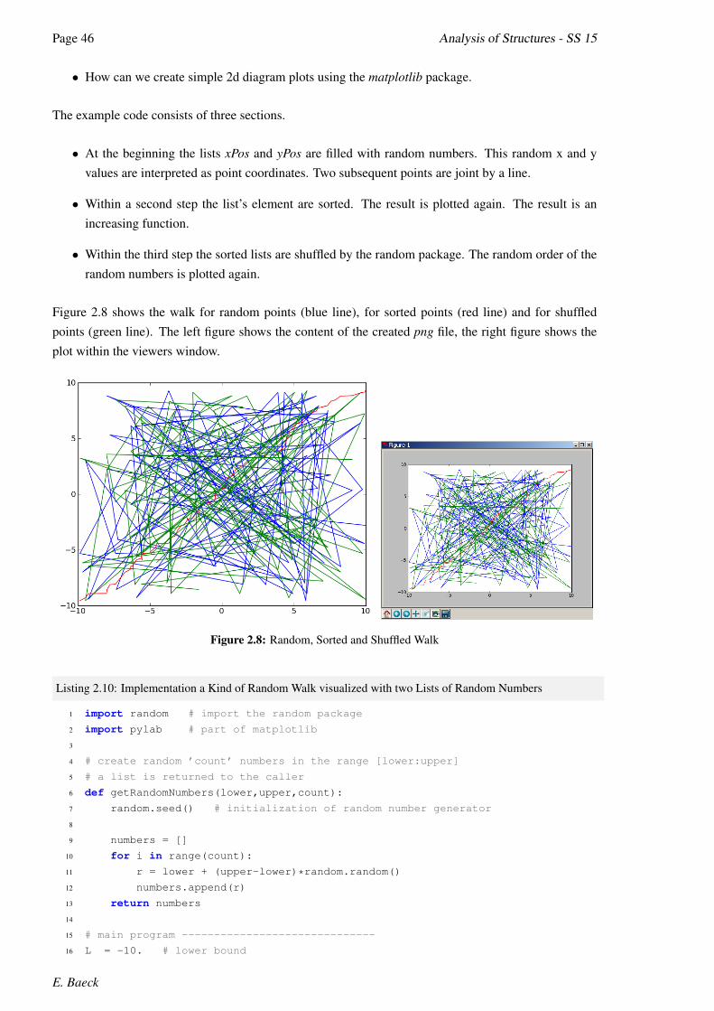
Page 46 Analysis of Structures - SS 15
• How can we create simple 2d diagram plots using the matplotlib package.
The example code consists of three sections.
• At the beginning the lists xPos and yPos are filled with random numbers. This random x and yvalues are interpreted as point coordinates. Two subsequent points are joint by a line.
• Within a second step the list’s element are sorted. The result is plotted again. The result is anincreasing function.
• Within the third step the sorted lists are shuffled by the random package. The random order of therandom numbers is plotted again.
Figure 2.8 shows the walk for random points (blue line), for sorted points (red line) and for shuffledpoints (green line). The left figure shows the content of the created png file, the right figure shows theplot within the viewers window.
Figure 2.8: Random, Sorted and Shuffled Walk
Listing 2.10: Implementation a Kind of Random Walk visualized with two Lists of Random Numbers
1 import random # import the random package
2 import pylab # part of matplotlib
3
4 # create random ’count’ numbers in the range [lower:upper]
5 # a list is returned to the caller
6 def getRandomNumbers(lower,upper,count):
7 random.seed() # initialization of random number generator
8
9 numbers = []
10 for i in range(count):
11 r = lower + (upper-lower)*random.random()
12 numbers.append(r)
13 return numbers
14
15 # main program ------------------------------
16 L = -10. # lower bound
E. Baeck

2.17. DATE, TIME AND TIMESPAN Page 47
17 U = +10. # upper bound
18 xN = 100 # number of randoms
19
20 # random positions
21 xPos = getRandomNumbers(L,U,xN) # ...in x-direction
22 yPos = getRandomNumbers(L,U,xN) # ...in y-direction
23
24 # creating plot of original random values xPos/yPos
25 pylab.plot(xPos,yPos,"b")
26
27 # sort the random values
28 xPos.sort()
29 yPos.sort()
30
31 # creating plot of sorted values xPos/yPos
32 pylab.plot(xPos,yPos,"r")
33
34 # create a random order
35 random.shuffle(xPos)
36 random.shuffle(yPos)
37
38 # creating plot of the shuffeled values xPos/yPos
39 pylab.plot(xPos,yPos,"g")
40
41 # save the plot in a figure using an png-format
42 pylab.savefig("RandomWalk.png")
43
44 # plot a figure in the matplotlib viewer
45 pylab.show()
46
47 # at the end we should close the plot,
48 # to avoid memory effects
49 pylab.close()
2.17 Date, Time and Timespan
Date and time functions in common are very important and therefor Python supports this with a stan-dard package datetime. Within this package you will find some very simple and powerful objects andfunctions.
The package is loaded with the following statement. We load from datetime the subpackage datetimeand set the alias name time. The second line shows, how to get the actual time. The datetime objectcontents from the left to the right the year, the month, the day, the hour, the minutes, the seconds andthe microseconds. Because the computer does not support microseconds but milliseconds the measuredmilliseconds are multiplied with the factor 1000.
1 >>> from datetime import datetime as time
2 >>> time.now()
3 datetime.datetime(2010, 11, 4, 19, 25, 33, 15000)
To implement some performance checking code it is very useful to have a timespan, which is the dif-ference of two datetime objects. The timespan object is called timedelta and is as well an object of thedatetime package.
8.5.2018

Page 48 Analysis of Structures - SS 15
If we now want to check the performance of a code snippet, we will implement the following code.First we have to import the datetime package. Then we get the actual time and assign this object to thevariable t1. Then the code to check follows. Within a last step we again create a datetime object callingthe time.now() function and assigning the object to the variable t2. If we subtract t1 from t2 wewill get a timedelta object. The timedelta objects contents the number of days, the number of secondsand the number of microseconds of the time difference.
1 from datetime import datetime as time
2 t1 = time.now()
3 ... our code snippet ...
4 t2 = time.now()
5 t3 = t2 -t1
6 print t3
7 >>> datetime.timedelta(0, 12, 906000)
If we want to have the time difference in seconds, we have to write a little function, which adds all thistime parts in the unit second. If we suppose, that T is a valid timedelta object, we extract the seconds withthe seconds attribute and assign it to our seconds variable. The next part handles the microseconds.We divide them by 106 and add the part to the seconds variable. The last part calculates the seconds ofthe given hours and add this value to our second variable. The value is returned to the caller.
1 def getTimeSpanInSeconds(T):
2 secs = float(T.seconds)
3 secs += float(T.microseconds)/1.e6
4 secs += float(t.days)*24.*60.*60.
5 return secs
One very important application of the timedelta object is the measurement of a program’s performance.The next example shows how to investigate the performance of the creation of a tuple and the creation ofa list. Here we apply the above discussed function getTimeSpanInSeconds.
Listing 2.11: Implementation of a Performance-Checker
1 # we need the datetime package
2 from datetime import datetime as time
3
4 # calculating the timespan in floats
5 def getTimeSpanInSeconds(T):
6 t = float(T.seconds)
7 t+= float(T.microseconds)/1.e6
8 t+= float(T.days)*24.*60.*60
9 return t
10
11
12 nX = 100000 # number of entities to create
13 T = () # empty tuple
14 L = [] # empty list
15
16 # create a tuple with nX items
17 t1 = time.now()
18 for i in range(nX):
19 T += (i,)
20 t2 = time.now()
21
22 sT = getTimeSpanInSeconds(t2-t1) # and calculate the timespan
E. Baeck
2.18. WORKING WITH FILES Page 49
23 print "Creation of a tuple with %d items: %.3fs" % (nX,sT)
24
25 # create a list with nX items
26 t1 = time.now()
27 for i in range(nX):
28 L += [i,]
29 t2 = time.now()
30 sL = getTimeSpanInSeconds(t2-t1) # and calculate the timespan
31 print "creation of a list with %d items: %.3fs" % (nX,sL)
32
33 # convert the list into a tuple
34 t1 = time.now()
35 TL = tuple(L)
36 t2 = time.now()
37 sTL= getTimeSpanInSeconds(t2-t1) # and calculate the timespan
38 print "Create tuple from list: %.3fs" % sTL
The console output on a one year old double processor notebook is given below. You see that it is verywasteful to create a tuple with a lot of items concatenating them with a += operator. On the other hand alist with the some number of items is created in no time. And the conversion of a list into a tuple costsnothing. So we can resume the the creation of a very large tuple should be done by creating a list andconverting it into a tuple.
1 c:\CM\Cm-AoS\WS1011\Python>Timecheck1.py
2 Creation of a tuple with 100000 items: 33.297s
3 Creation of a list with 100000 items: 0.063s
4 Create tuple from list: 0.000s
2.18 Working with Files
A file is a sequence of bytes written to an external media like a hard disk, a CD or an USB stick. A file’sbytes are indexed with an integer. So the the fist byte of a file has the index 0 and the second byte theindex 1 and so on. A text file is structured with a line break character \n. If a text line should be read,the io12 system reads all the bytes up to the next line break.
Python as a lot of functions which are able to handle every situation concerning files. So files can becreated. We can read data from a file or write data into a file. We can close a file. We can delete a file orchange it’s permissions.
2.18.1 Open a File
Within Python a file is an object an has a lot of attributes and methods (see also the next section). Theaccess to a file is initialized with the file constructor. The file constructor needs the name of the file andthe type of access. The file access type is like C’s access type of the function fopen13. The type ’r’ isused to read from a file, the type ’w’ is used to create a new file for writing. An old still existing filewill be deleted. The type ’a’ is used to write appending to an existing or a new file. If we want to readfrom and write into a file the type ’w+’ can be used.
12io means input output.13The function fopen is C’s classical function to open a file. The return will be a pointer to a FILE structure.
8.5.2018

Page 50 Analysis of Structures - SS 15
1 f = file(<filename>,<access-type>)
2 ...
3 ... example ...
4 ...
5 f = file("myfile.txt", "w")
2.18.2 Write Data into a File
The file method write writes a stream of bytes into a file. In contrast to the print function the write methodadds no carriage return to the file. If a line of text should be written, the text should be closed with an \ncharacter.
1 #> f.write(<byte-stream>)
2 #> ...
3 #> ... example ...
4 #> ...
5 f.write("This is my first line\n")
2.18.3 Close a File
After the usage of a file, the file should be closed.
1 #> f.close()
2 #> ...
3 #> ... example ...
4 #> ...
5 f.open("log.txt","a")
6 f.write("Write a little log line\n")
7 f.close()
2.18.4 Read Data from a Text File
A frequently problem is parsing an input file for some control data. This we can do with a statementwhich reads the entire file into a list container using the method readlines. If we have read this lines thenwe can iterate this container using the for statement. Doing this we will get line by line.
A line is a string which is terminated by a carriage return character. This string we can split up intopieces using white spaces (blanks and tabs) as separators.
Listing 2.12: Read Data from a Text File
1 # import the fileinput package
2 import fileinput
3
4 h = -1. # initialize H value
5 w = -1. # initialize W value
6
7 file = open("data.in") # open the file
8 lines = file.readlines() # read entire content
9 file.close() # close the file
10 print lines # check the container
11
E. Baeck

2.18. WORKING WITH FILES Page 51
12 for line in lines: # iterate all lines
13
14 words = line.split() # split up into pieces
15
16 if len(words) < 1: continue # ignore blank lines
17 if words[0] == "#": continue # ignore comment lines
18
19 if words[0] == "H": # evaluate H key
20 h = float(words[1])
21
22 elif words[0] == "W": # evaluate H key
23 w = float(words[1])
24
25 print "h = %8.2f" % h # print H value
26 print "w = %8.2f" % w # print W value
In our example we want to read and analyze the input file data.in (see listing 2.13).
Listing 2.13: Key Value Input Control File
1 # this is a comment
2 # format is key - value like
3 H 100.
4 W 10.
If we run the script 2.12 we will get the console output 2.14. In line 1 we can see, that readlines willcreate a list container (see square brackets).
Listing 2.14: Consol Output
1 [’# this is a comment\n’, ’# format is key - value like\n’, ’H 100.\n’, ’W
10.\n’]
2 h = 100.00
3 w = 10.00
8.5.2018
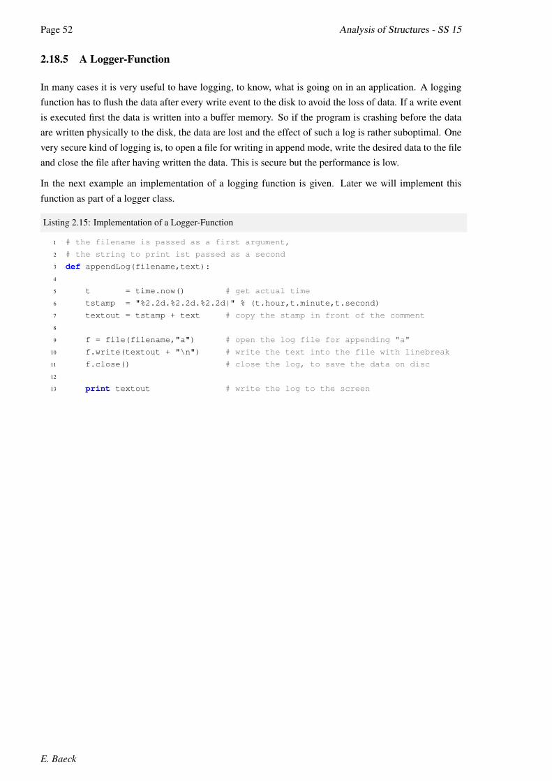
Page 52 Analysis of Structures - SS 15
2.18.5 A Logger-Function
In many cases it is very useful to have logging, to know, what is going on in an application. A loggingfunction has to flush the data after every write event to the disk to avoid the loss of data. If a write eventis executed first the data is written into a buffer memory. So if the program is crashing before the dataare written physically to the disk, the data are lost and the effect of such a log is rather suboptimal. Onevery secure kind of logging is, to open a file for writing in append mode, write the desired data to the fileand close the file after having written the data. This is secure but the performance is low.
In the next example an implementation of a logging function is given. Later we will implement thisfunction as part of a logger class.
Listing 2.15: Implementation of a Logger-Function
1 # the filename is passed as a first argument,
2 # the string to print ist passed as a second
3 def appendLog(filename,text):
4
5 t = time.now() # get actual time
6 tstamp = "%2.2d.%2.2d.%2.2d|" % (t.hour,t.minute,t.second)
7 textout = tstamp + text # copy the stamp in front of the comment
8
9 f = file(filename,"a") # open the log file for appending "a"
10 f.write(textout + "\n") # write the text into the file with linebreak
11 f.close() # close the log, to save the data on disc
12
13 print textout # write the log to the screen
E. Baeck
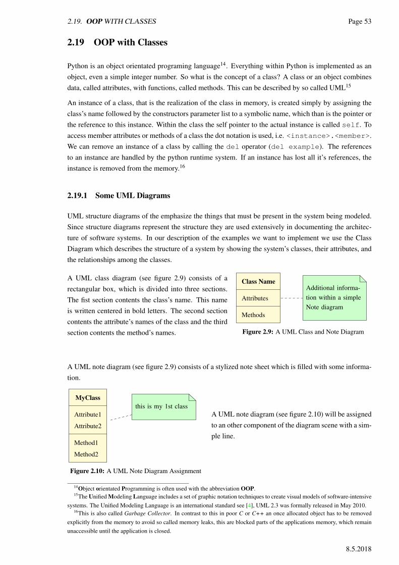
2.19. OOP WITH CLASSES Page 53
2.19 OOP with Classes
Python is an object orientated programing language14. Everything within Python is implemented as anobject, even a simple integer number. So what is the concept of a class? A class or an object combinesdata, called attributes, with functions, called methods. This can be described by so called UML15
An instance of a class, that is the realization of the class in memory, is created simply by assigning theclass’s name followed by the constructors parameter list to a symbolic name, which than is the pointer orthe reference to this instance. Within the class the self pointer to the actual instance is called self. Toaccess member attributes or methods of a class the dot notation is used, i.e. <instance>.<member>.We can remove an instance of a class by calling the del operator (del example). The referencesto an instance are handled by the python runtime system. If an instance has lost all it’s references, theinstance is removed from the memory.16
2.19.1 Some UML Diagrams
UML structure diagrams of the emphasize the things that must be present in the system being modeled.Since structure diagrams represent the structure they are used extensively in documenting the architec-ture of software systems. In our description of the examples we want to implement we use the ClassDiagram which describes the structure of a system by showing the system’s classes, their attributes, andthe relationships among the classes.
Class Name
Attributes
Methods
Additional informa-tion within a simpleNote diagram
Additional informa-tion within a simpleNote diagram
Figure 2.9: A UML Class and Note Diagram
A UML class diagram (see figure 2.9) consists of arectangular box, which is divided into three sections.The fist section contents the class’s name. This nameis written centered in bold letters. The second sectioncontents the attribute’s names of the class and the thirdsection contents the method’s names.
A UML note diagram (see figure 2.9) consists of a stylized note sheet which is filled with some informa-tion.
MyClass
Attribute1
Attribute2
Method1
Method2
this is my 1st classthis is my 1st class
Figure 2.10: A UML Note Diagram Assignment
A UML note diagram (see figure 2.10) will be assignedto an other component of the diagram scene with a sim-ple line.
14Object orientated Programming is often used with the abbreviation OOP.15The Unified Modeling Language includes a set of graphic notation techniques to create visual models of software-intensive
systems. The Unified Modeling Language is an international standard see [4], UML 2.3 was formally released in May 2010.16This is also called Garbage Collector. In contrast to this in poor C or C++ an once allocated object has to be removed
explicitly from the memory to avoid so called memory leaks, this are blocked parts of the applications memory, which remainunaccessible until the application is closed.
8.5.2018
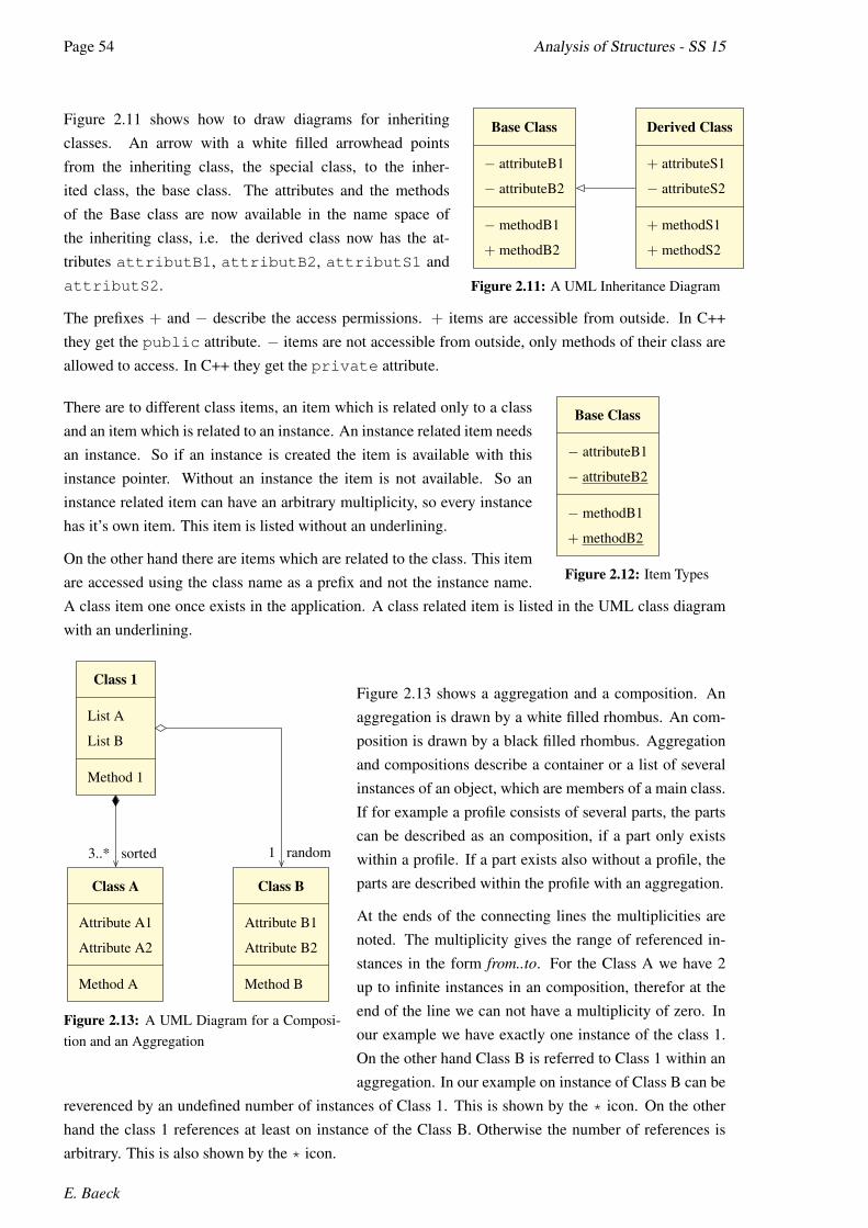
Page 54 Analysis of Structures - SS 15
Base Class
− attributeB1
− attributeB2
− methodB1
+ methodB2
Derived Class
+ attributeS1
− attributeS2
+ methodS1
+ methodS2
Figure 2.11: A UML Inheritance Diagram
Figure 2.11 shows how to draw diagrams for inheritingclasses. An arrow with a white filled arrowhead pointsfrom the inheriting class, the special class, to the inher-ited class, the base class. The attributes and the methodsof the Base class are now available in the name space ofthe inheriting class, i.e. the derived class now has the at-tributes attributB1, attributB2, attributS1 andattributS2.
The prefixes + and − describe the access permissions. + items are accessible from outside. In C++they get the public attribute. − items are not accessible from outside, only methods of their class areallowed to access. In C++ they get the private attribute.
Base Class
− attributeB1
− attributeB2
− methodB1
+ methodB2
Figure 2.12: Item Types
There are to different class items, an item which is related only to a classand an item which is related to an instance. An instance related item needsan instance. So if an instance is created the item is available with thisinstance pointer. Without an instance the item is not available. So aninstance related item can have an arbitrary multiplicity, so every instancehas it’s own item. This item is listed without an underlining.
On the other hand there are items which are related to the class. This itemare accessed using the class name as a prefix and not the instance name.A class item one once exists in the application. A class related item is listed in the UML class diagramwith an underlining.
sorted3..* random1
Class 1
List A
List B
Method 1
Class A
Attribute A1
Attribute A2
Method A
Class B
Attribute B1
Attribute B2
Method B
Figure 2.13: A UML Diagram for a Composi-tion and an Aggregation
Figure 2.13 shows a aggregation and a composition. Anaggregation is drawn by a white filled rhombus. An com-position is drawn by a black filled rhombus. Aggregationand compositions describe a container or a list of severalinstances of an object, which are members of a main class.If for example a profile consists of several parts, the partscan be described as an composition, if a part only existswithin a profile. If a part exists also without a profile, theparts are described within the profile with an aggregation.
At the ends of the connecting lines the multiplicities arenoted. The multiplicity gives the range of referenced in-stances in the form from..to. For the Class A we have 2up to infinite instances in an composition, therefor at theend of the line we can not have a multiplicity of zero. Inour example we have exactly one instance of the class 1.On the other hand Class B is referred to Class 1 within anaggregation. In our example on instance of Class B can be
reverenced by an undefined number of instances of Class 1. This is shown by the * icon. On the otherhand the class 1 references at least on instance of the Class B. Otherwise the number of references isarbitrary. This is also shown by the * icon.
E. Baeck

2.19. OOP WITH CLASSES Page 55
2.19.2 Implementation of Classes in Python
ClassX
+ attributeX1
− attributeX2
− methodX1
+ methodX2
ClassY
+ attributeY1
− attributeY2
− methodY1
+ methodY2
ClassZ
+ attributeZ1
− attributeZ2
+ methodZ1
+ methodZ2
Figure 2.14: Some Classes
Classes are implemented in Python with the keywordclass. The class key is followed by the name of theclass, which we find in the upper section of the class dia-gram. If a class inherits from other classes, it’s called sub-class. Then the subclass’s name is followed by a comma sep-arated list of classes to inherit from. This classes are calledbase classes, superclasses or parent classes. So we have thefollowing syntax, if your class ClassZ should inherit fromClassX and ClassY. The implementation of the class isindented like a function’s code.
1 class ClassZ(ClassX, ClassY):
2 ..
3 class implementation
4 ..
2.19.2.1 Class Constructor
The constructor of a class is called if an instance is created. A constructor is a function, i.e. method ofa class, having a fixed name. The constructor defines the interface to the class, if an instance should becreated.
The following code shows the constructor of class ClassZ and how to create it’s instance. The nameof the constructor is __init__. The leading two underscores set the constructor to private, i.e. thismethod is hidden and is not allowed to call from outside. We also should notice, that an instance referencein Python is passed with the key self. This parameter, the first in the implementation, is not explicitlypassed (see line 9). Only the the real parameters should be passed in the call. A further thing to mentionis, that instance attributes are only created, if an assignment is done.17
1 class ClassZ(ClassX, ClassY):
2
3 def __init__(self,par1,par2):
4 self.attributeZ1 = par1
5 self.__attributeZ1 = par2
6
7 ..
8
9 c = ClassZ(1,2)
17In a compiled language like C++ or FORTRAN a variable, an attribute or a method are created in compile time, they areavailable already at start up.
8.5.2018

Page 56 Analysis of Structures - SS 15
2.19.2.2 Class Destructor
The destructor of a class is called if an instance is deleted with the del command, which means is freedfrom the memory. The destructor is a functions, i.e. method of a class, having a fixed name.
The following code shows the destructor of class ClassZ. The name of the destructor is __del__. Theleading two underscores set the destructor to private, i.e. this method is hidden and is not allowed to callfrom outside. We also should notice, that an instance reference in Python is passed with the key self.The destructor only has one parameter the instance reference. The example shows like before how wecreate an instance of the class ClassZ and how to free it. If we free this instance, the instance’s method__del__ is executed and gives us a goodby.
1 class ClassZ(ClassX, ClassY):
2
3 ...
4
5 def __del__(self):
6 print "goodby!"
7
8 ..
9
10 c = ClassZ(1,2)
11 del c
We should consider, that destructors can not handle exceptions.
E. Baeck

2.19. OOP WITH CLASSES Page 57
2.19.3 Implementation of a Time Stack Class
In section 2.17 we have discussed a little program which implements a time checker using a stack con-tainer. We can implement this problem in a much more clearer version, if we do it in terms of the OOPapproach. The class TimeCheck, which is introduced, encapsulates the time stack list and the log filesname as attributes and the following methods.
• set reads the actual time with the datetime.now() and pushes it onto the time stack.
• get reads the actual time with the datetime.now(), pops the the last time object from the stack andcalculates the timespan. The timespan is optionally printed into the console window or into a logfile.
• getTime calculates the seconds in floats form the passed timedelta object.
The main program, which is used to discuss the class follows the steps of the classical implementationof the problem discussed in section 2.17. We first create an empty tuple and an empty list. Than wecreate the TimeCheck instance18 simple by assigning it’s name to a variable (s = TimeCheck()). Topush a time object onto the stack, we call the class’s member function Set. So, if we want to check theperformance of a code, we first call the Set method and after having executed the code, we call the Getmethod. The Get method will print the comment and will return the used seconds of execution time infloats. The simplest kind of an implementation is the implementation in the file of the main program.This you can see in the following example.
A UML diagram of the class TimeCheck is given in figure 2.15.
TimeCheck
+ self. log: name of the log file
+ self. stack: stack list
+ self. init (..): contructor
+ self.set(..): push a time
+ self.getTime(..): calculate seconds
+ self.get(..): pop a time
The class TimeCheck contents all the data andfunctions to use a time stack and to get thetime-span information in a proper float format.The class is able to present a formated outputof the measured time-spans.
The class TimeCheck contents all the data andfunctions to use a time stack and to get thetime-span information in a proper float format.The class is able to present a formated outputof the measured time-spans.
Figure 2.15: UML-Diagram of the TimeCheck Class
18A physical created object in memory of a class is called instance of a class.
8.5.2018

Page 58 Analysis of Structures - SS 15
Listing 2.16: Implementation of a Performance-Checker-Class
1 ’’’
2 Class to investigate the timespan, to measure the performance
3 by implementing a time stack container
4 ’’’
5 # - module - member alias
6 from datetime import datetime as time # we need the datetime package
7
8 class TimeCheck(): # class name
9
10 # constructor
11 def __init__(self,log = "timestack.log"):
12 self._stack = [] # empty list
13 self._log = log # set the logfile’s name
14
15 # set up the actual time and push it onto the stack
16 def set(self):
17 self._stack.append(time.now())
18
19 # calculate the timespan in float
20 def getTime(self,T):
21 s = float(T.microseconds)/1.e6 +float(T.seconds) +float(T.days)*24.*60.*60.
22 return s
23
24 # calculate the timespan with a stack object
25 def get(self,text = ""):
26
27 # get the stack length
28 items = len(self._stack)
29
30 # assert(items > 0) # to assert, that there is a time object
31 # stored in stack (alternative solution)
32 if items < 1:
33 print "*** Error: timestack empty!"
34 return
35
36 tStart = self._stack.pop() # pop the time object from the stack
37 tEnd = time.now() # get the end time
38 tDel = self.getTime(tEnd -tStart) # calculate the timedelta in floats
39
40 # we have an maximal indent of 6 columns
41 indent = 6
42 space1 = "" # leading characters for level indent
43 space2 = "" # trailed characters to aling the comment
44
45 # set up indent text
46 for i in range(items-1): space1 += "." # fill in dots
47 for i in range(indent -items): space2 += " " # fill in white spaces
48
49 # print comment if given
50 if len(text) > 0:
51 textout = "%s %8.3f%s: %s" % (space1,tDel,space2,text)
52
53 # comment to the screen
54 print textout
E. Baeck

2.19. OOP WITH CLASSES Page 59
55
56 # logging the comment
57 f = file(self._log,"a")
58 f.write(textout + "\n")
59 f.close()
60
61 return tDel # return the seconds in floats
62
63 # application of the TimeCheck class
64 print ">> Start.."
65 nX = 50000
66 T = () # empty tuple
67 L = [] # empty list
68
69 # create the timecheck object
70 s = TimeCheck()
71
72 # check the total performance
73 s.set()
74
75 # check the performance of the tuples
76 s.set()
77 for i in range(nX): T+= (i,)
78 s.get("Creating %d item tuple." % nX)
79
80 # check the performance of the list
81 s.set()
82 for i in range(nX): L+= [i]
83 s.get("Creating %d item list." % nX)
84
85 # check the whole performance
86 s.get("total time")
If we run the program, we see that two time stamps are indented with one dot. This timestamps are setfor inner performance measurements, that is the time-stamp for the creation of the tuple and after thatthe time-stamp for the the creation of the list. The last time-stamp shows the total execution time and iscreated by the first push, i.e. the first Set call and the last pop, i.e. the last Get call.
1 >> Start..
2 . 8.282 : Creating 50000 item tuple.
3 . 0.016 : Creating 50000 item list.
4 8.329 : total time
8.5.2018

Page 60 Analysis of Structures - SS 15
E. Baeck
3
Python Projects
3.1 Newton, Step2
We have discussed the newton’s scheme in section 2.10. Within this section the project’s code will beextended by plot features. The function and it’s derivative as well as the path of iteration will be plottedusing the pylab package.
The following features are added to the implementation of newton’s scheme.
1. Import the pylab package.
2. The function getFunctionValues creates a list of the function values for the plot routine.
3. The function getFunctionDerivativeValues creates a list of the function’ derivative values for theplot routine.
4. The function newton will be extended by two lists, which should store the values of the iterationpath. After each iteration step, the x-value and it’s function value are stored for later drawings.
61

Page 62 Analysis of Structures - SS 15
A disadvantage of the first implementation in section 2.13.2 is, that the algorithm will fail, if a vanishingslope is found. With a simple work around we can solve this problem. We simple step aside as long as aminimum slope value is reached. The flow chart is given in figure 3.1.
Start
Initializing:x = x0; i = 0;
i ≥ imax NO ROOT!yes
Stop
Fx = f(x)
no
|Fx| ≤ ε ROOT: xyes
Stop
Fs = f ′(x)
no
|Fs| ≤ εx = x + ∆
i = i + 1
yes
x = x − FxFs
no
i = i + 1
Figure 3.1: Flow Chart for a Slope Insensitive Newton Implementation
Listing 3.1: Implementation of Newton’s-Algorithm, plotting the results
1 import pylab # plot a little (not used in this step)
2 from math import fabs as abs # import the fabs as abs
3
4 # implementation of the function of interest
5 def myF(x):
6 return x**2 -1.
7 # return x**10 -1. # check the extrem case
8 # return 0. # check the constant
9
10 # calculating the derivative
11 def fs(f,x,h=1.e-6):
12 h = float(h)
E. Baeck

3.1. NEWTON, STEP2 Page 63
13 x = float(x)
14 return (f(x+0.5*h) - f(x-0.5*h))/h
15
16 # implementation of a newton algorithm
17 def newton(f,x0,e=1.e-10,h=1.e-6,imax=1000):
18
19 error = None # initialize the error code with None
20
21 h = float(h) # we need some floats
22 e = float(e)
23 x1= float(x0) # x to interate
24 f1= None # initialize it for return
25
26 xL= [] # list for x-values
27 yL= [] # list for the function values for x
28 sL= [] # list for the slope values for x
29
30 i = 0 # iteration counter
31 while True:
32
33 # available iterations exceeded
34 if i >= imax:
35 error = "*** Error: no root found!"
36 break
37
38 # checking for roots
39 f0 = f(x1) # function’s value
40 xL.append(x1) # save x Value
41 yL.append(f0) # save the functions value
42 if abs(f0) < e:
43 f1 = fs(f,x1,h)
44 sL.append(f1) # save the last nslope value
45 break
46
47 # calculating the derivative
48 f1 = fs(f,x1,h)
49 sL.append(f1) # save the slope value
50
51 if abs(f1) < e:
52 x1 += 1.e2*h # little step aside
53 i += 1 # avoid dying with a vanishing slope
54 continue
55
56 # calculating the values for next iteration
57 x1 -= f0/f1
58
59 # increment the iteration counter
60 i+=1
61
62 # return the actual position, the function value
63 # and the functions slope, the number of performed
64 # iterations and the error code.
65 # index 0 1 2 3 4 5 6 7
66 return (x1,f0,f1,i,error,xL,yL,sL)
67
68 # creating a list of function values for a x-list
8.5.2018

Page 64 Analysis of Structures - SS 15
69 def getFunctionValues(xL,f):
70 yL = []
71 for x in xL:
72 y = f(x)
73 yL.append(y) # yL += [y]
74
75 return yL
76
77 # create a list of function’ derivative values
78 def getFunctionDerivateValues(xL,f):
79 yL = []
80 for x in xL:
81 y = fs(f,x)
82 yL.append(y)
83
84 return yL
85
86 # parameters of the problem
87 xl = -5. # lower bound
88 xu = 5. # upper bound
89 xc = 0.5 # increment
90
91 # visalization of the function and it’s derivative
92 # create the x-List
93 xList = pylab.arange(xl,xu,xc)
94
95 # create list of function’s values
96 yList = getFunctionValues(xList,Myf)
97 pylab.plot(xList,yList,’b’)
98
99 # create list of function’s derivative values
100 ysList = getFunctionDerivateValues(xList,Myf)
101 pylab.plot(xList,ysList,’g’)
102
103 # the function newton is called with standard parameters
104 # we pass the function of interest and a supposed start
105 # position
106 x0 = 0.
107 res = newton(Myf,x0)
108
109 # the returned tuple is printed into the console window
110 print "\n> next run"
111 print "x0 = %f" % x0 # starting value
112 print "x = %f" % res[0] # last x value
113 print "f(x) = %f" % res[1] # last f(x) value
114 if res[2] is not None:
115 print "f’(x) = %f" % res[2] # last f’(x) value
116 print "i = %d" % res[3] # number of iterations
117 if res[4] is not None:
118 print "%s" % res[4] # error message
119 if len(res[5]) > 0:
120 print "--------------x -----------f(x) ----------f’(x)"
121 for i in range(len(res[5])):
122 print "%15.6e %15.6e %15.6e" % (res[5][i],res[6][i],res[7][i])
123 print "--- end of code ---\n"
124
E. Baeck

3.1. NEWTON, STEP2 Page 65
125 # plot the iteration path
126 pylab.plot(res[5],res[6],’rp’)
127
128 # output of plot data
129 pylab.grid(True) # show grid lines
130 pylab.savefig("NewtonStep2.png")
131
132 # - show plot data
133 pylab.show()
After the output lists are created the lists are passed to the plot post-processor by the plot method ofPyLab. After enabling the grid the plot data are written in a graphic file and are visualized in the PyLabviewer application.
Figure 3.2 shows the iteration path for the equation f(x) = x2 − 1 with an starting value of 4 with reddots.
Figure 3.2: Newton’s Iteration Path starting with 4
If we would start our calculation with a starting value of 0, we know that the slope will vanish. If wenow step aside with the precision of our numerical derivative, we will get the following iteration path.
1 x0 = 0.000000
2 x = 1.000000
3 f(x) = 0.000000
4 f’(x) = 2.000000
5 i = 18
6 --------------x -----------f(x) ----------f’(x)
7 0.000000e+00 -1.000000e+00 0.000000e+00
8 1.000000e-04 -1.000000e+00 2.000000e-04
9 5.000000e+03 2.500000e+07 1.000000e+04
10 2.500001e+03 6.250002e+06 5.000003e+03
11 1.250001e+03 1.562501e+06 2.500002e+03
12 6.250008e+02 3.906250e+05 1.250002e+03
8.5.2018

Page 66 Analysis of Structures - SS 15
13 3.125012e+02 9.765602e+04 6.250025e+02
14 1.562522e+02 2.441375e+04 3.125044e+02
15 7.812931e+01 6.103189e+03 1.562586e+02
16 3.907105e+01 1.525547e+03 7.814211e+01
17 1.954832e+01 3.811370e+02 3.909665e+01
18 9.799739e+00 9.503489e+01 1.959948e+01
19 4.950891e+00 2.351133e+01 9.901783e+00
20 2.576438e+00 5.638031e+00 5.152875e+00
21 1.482285e+00 1.197170e+00 2.964570e+00
22 1.078460e+00 1.630751e-01 2.156919e+00
23 1.002854e+00 5.716204e-03 2.005708e+00
24 1.000004e+00 8.122320e-06 2.000008e+00
25 1.000000e+00 1.649347e-11 2.000000e+00
26 --- end of code ---
We see that due to the very small slope, the resulting jump in the iteration is very large, so that we needsome iterations more to get the root. If we would do this on a very flat function like f(x) = x10− 1, wehave to count the steps, to avoid the programs hanging. The function is as flat that the number of smallsteps to get out of the trap will increase to a nearly infinite number.
Figure 3.2 shows the iteration path for the equation f(x) = x2 − 1 with an starting value of 0 with reddots.
Figure 3.3: Newton’s Iteration Path starting vom 0
E. Baeck
3.2. PROFILES, THIN WALLED APPROACH Page 67
3.2 Profiles, Thin Walled Approach
In this section we will implement a class hierarchy to model a profile’s data. We will implement logginginto file and screen in a common base class and we will implement the thin walled approach to analyzeand calculate the profile’s section properties.
Applying the Thin Walled Approximation every part of a section will be approximated by a line with agiven thickness. This approach is similar to the approach modeling a three dimensional shell structure.Hereby we use shell elements, i.e. faces, with a given thickness. The lines like the shell elements in FEwill connect nodes or points.
So if we want to build up a calculation model for our thin-walled section, we need something like linesand points. Lines are called Elments and Points are called Nodes like in the case of programs. In ourcase we introduce two classes.
• The class Node describes the contour point of elements. In our case we have the end points oflines in two dimensions.
• The class Element describes the connection between nodes. In our case we connect points withlines so that we have to specify the thickness of the line, ie. the connection.
Further we introduce a class Base, which should content all common features. A general profile thenwill be described by the class Profile. This class can therefore be considered as a container for our pointsand lines as well as the class which should perform all calculations. To show the power of inheritance weintroduce a derived profile class, which is called UProfile. This class will describe all U-profiles withtheir geometric parameters. Based on our class Profile this class will be able to calculate all sectionvalues based on the given parameter set. All details, i.e. points and lines are encapsulated in it’s baseclass.
3.2.1 A General Base Class
If we want to use the code of an existing class within a new class, we can inherit this old class and useit as a base class. That means, that the new class contents also the attributes and the methods of the oldone. A base class is used in the class statement as an argument. A class can inherit more than one class.In our case everything is derived from our general base class called Base.
The class Base should content logging for all classes. This class should also be able to count all cre-ated instances of the developed application. The output method for all classes should be the methodAppendLog, i.e. this method will be inherited by all classes of our project. The classes UML diagramis given in figure 3.4.
The class Base counts the instances using the global class attribute __count. A common loggingmethod is implemented. So the name of the log file is implemented as a class method (not an instancemethod) __log. The method appendLog is implemented as a general logging function. The actualtime is called an copied as heading for our logging comment. Then the completed logging text is writteninto the log file and into the screen.
8.5.2018

Page 68 Analysis of Structures - SS 15
Base
− log: global log file name
− count: global instance counter
− self. init (..): constructor
+ self.appendLog(..): write to log
The class Base contents commonfeatures which are used in everyclass.
The class Base contents commonfeatures which are used in everyclass.
Figure 3.4: The Base Class of all TWD Classes
The implementation of the class Base is given in listing 3.2.
Listing 3.2: Implementation of a Base-Class
1 ’’’
2 the Base class of all TWA-classes
3 ’’’
4 # import some packages
5 # |package
6 # | | select the item to import
7 # | | | alias name
8 from datetime import datetime as time
9
10 class Base:
11 __log = "profiles.log" # class attribut, type private
12 __count = 0 # class attribut, instance counter
13
14 # construtor
15 # |instance pointer
16 # | |optional parameter
17 def __init__(self,log = ""):
18 Base.__count += 1 # increment the counter
19 if len(log) > 0: Base.__log = log # set a new log-file name
20
21 # print the instance counter value
22 self.appendLog(">> instance %d created!" % Base.__count)
23
24 # print a message into the log file and to the console
25 # | instance pointer
26 # | | text to print
27 def appendLog(self,text):
28 t = time.now() # get the time
29 tstamp = "%2.2d.%2.2d.%2.2d |" % (t.hour,t.minute,t.second)
30 textout = tstamp + text # text to print
31
32 # use the file object to print with the append mode "a"
33 f = file(Base.__log,"a")
34 f.write(textout+"\n") # write text
35
36 print textout
37
38 # destructor
39 def __del__(self):
40 self.appendLog("instance %d deleted" % Base.__count)
41 Base.__count -= 1 # decrement the counter
E. Baeck
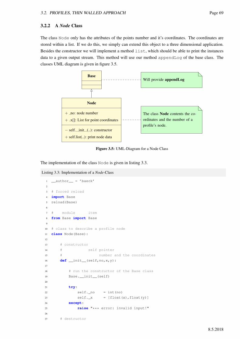
3.2. PROFILES, THIN WALLED APPROACH Page 69
3.2.2 A Node Class
The class Node only has the attributes of the points number and it’s coordinates. The coordinates arestored within a list. If we do this, we simply can extend this object to a three dimensional application.Besides the constructor we will implement a method list, which should be able to print the instancesdata to a given output stream. This method will use our method appendLog of the base class. Theclasses UML diagram is given in figure 3.5.
BaseWill provide appendLogWill provide appendLog
Node
+ no: node number
+ x[]: List for point coordinates
− self. init (..): constructor
+ self.list(..): print node data
The class Node contents the co-ordinates and the number of aprofile’s node.
The class Node contents the co-ordinates and the number of aprofile’s node.
Figure 3.5: UML-Diagram for a Node Class
The implementation of the class Node is given in listing 3.3.
Listing 3.3: Implementation of a Node-Class
1 __author__ = ’baeck’
2
3 # forced reload
4 import Base
5 reload(Base)
6
7 # module item
8 from Base import Base
9
10 # class to describe a profile node
11 class Node(Base):
12
13 # constructor
14 # self pointer
15 # number and the coordinates
16 def __init__(self,no,x,y):
17
18 # run the constructor of the Base class
19 Base.__init__(self)
20
21 try:
22 self._no = int(no)
23 self._x = [float(x),float(y)]
24 except:
25 raise "*** error: invalid input!"
26
27 # destructor
8.5.2018

Page 70 Analysis of Structures - SS 15
28 def __del__(self):
29 pass
30
31 # list the node content
32 def list(self):
33 self.appendLog("node %d, x = %10.4f, y = %10.4f" % \
34 (self._no,self._x[0],self._x[1]))
3.2.3 Testing the Node Class
In our testing environment we simple import the Node module. Than we create a Node instance and listit’s data. After that we delete the instance and we try to print it again.
The implementation of the testing environment is given in listing 3.4.
Listing 3.4: Implementation of a Node-Testing Environment
1 ’’’
2 checking the Node class
3 ’’’
4 import Node # we have to be sure
5 reload(Node) # that we check the current file
6
7 from Node import Node # import the Node class
8
9 n = Node(3,1.,2.) # we create a point
10 n.listData() # and list it’s value
11
12 # delete the instance
13 print n # let’s print the Nodes address
14 del n # and than we delete the instance
15 print n # try to print it again
The output of our test application is given in the following code. We see, that the Base class constructorshows, that a new instance is created. The next line shows the output of Node’s list method followedby the simple instance print, which shows the address of the instance. Than the instance is explicitlydeleted, so that the destructor of the Base class shows that one instance is deleted. Because the addressof the instance after deleting is invalid, the program will crash with a trace back message. The line (line15) is given and the message shows us, that at this moment there is no valid variable called p.
1 15.49.12 |>> instance 1 created!
2 15.49.12 | point 3, y = 1.000, z = 2.000
3 <Node.Node instance at 0x031AE300>
4 15.49.12 |instance 1 deleted
5 Traceback (most recent call last):
6 File "C:\Python27\Lib\site-packages\Pythonwin\pywin\framework\scriptutils.py",
7 line 326, in RunScript
8 exec codeObject in __main__.__dict__
9 File "C:\UniDue\CM\Cm-AoS\AOS-BookOfExamples\Py\Code\Profiles\NodeApp.py",
10 line 15, in <module>
11 print p # try to print it again
12 NameError: name ’p’ is not defined
E. Baeck

3.2. PROFILES, THIN WALLED APPROACH Page 71
3.2.4 An Element Class
The class Element will describe the connection between points and will describe further the type ofconnection. In the case of a line we will have the line’s thickness. Because in our case the properties ofthe profile, i.e. it’s area and moments, are given by the sum over the element’s contribution (see sectionB), we put the code to calculate this properties into the element’s class. If we do so, the element mustknow everything about it’s points, i.e. the numbers of the points are not sufficient to have success. Sowe store the point’s instance pointers and not there number in our element. The classes UML diagram isgiven in figure 3.6.
The element can be considered as a container for Node instance pointers too. This is shown within thediagram using the composition link to the class Node. The cardinality in our case is exactly two. If wewould introduce faces too for the thick-walled case, the cardinality can also be greater then two.
2..*
Base
Element
+ no: element number
+ n[]: list of point instance pointers
+ t: line’s thickness
− self. init (..): constructor
+ self.getL(): get line’s length
+ self.getA(): get area
+ self.getS(): get static moments
+ self.getI(): get moments of inertia
+ self.list(..): print element data
The class Element contents theelement’s point data.The class Element contents theelement’s point data.
Node
+ no: node number
+ x[]: List for point coordinates
− self. init (..): constructor
+ self.list(..): print node data
Figure 3.6: UML-Diagram for a Element Class
8.5.2018
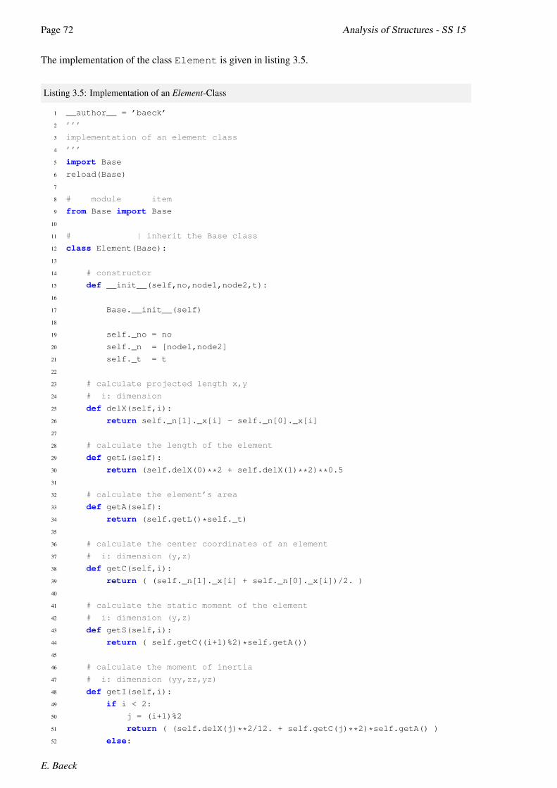
Page 72 Analysis of Structures - SS 15
The implementation of the class Element is given in listing 3.5.
Listing 3.5: Implementation of an Element-Class
1 __author__ = ’baeck’
2 ’’’
3 implementation of an element class
4 ’’’
5 import Base
6 reload(Base)
7
8 # module item
9 from Base import Base
10
11 # | inherit the Base class
12 class Element(Base):
13
14 # constructor
15 def __init__(self,no,node1,node2,t):
16
17 Base.__init__(self)
18
19 self._no = no
20 self._n = [node1,node2]
21 self._t = t
22
23 # calculate projected length x,y
24 # i: dimension
25 def delX(self,i):
26 return self._n[1]._x[i] - self._n[0]._x[i]
27
28 # calculate the length of the element
29 def getL(self):
30 return (self.delX(0)**2 + self.delX(1)**2)**0.5
31
32 # calculate the element’s area
33 def getA(self):
34 return (self.getL()*self._t)
35
36 # calculate the center coordinates of an element
37 # i: dimension (y,z)
38 def getC(self,i):
39 return ( (self._n[1]._x[i] + self._n[0]._x[i])/2. )
40
41 # calculate the static moment of the element
42 # i: dimension (y,z)
43 def getS(self,i):
44 return ( self.getC((i+1)%2)*self.getA())
45
46 # calculate the moment of inertia
47 # i: dimension (yy,zz,yz)
48 def getI(self,i):
49 if i < 2:
50 j = (i+1)%2
51 return ( (self.delX(j)**2/12. + self.getC(j)**2)*self.getA() )
52 else:
E. Baeck

3.2. PROFILES, THIN WALLED APPROACH Page 73
53 return ( (self.delX(0)*self.delX(1)/12. + self.getC(0)*self.getC(1))
54 *self.getA() )
55
56 # list the elements data
57 def list(self):
58 self.appendLog("element %d: nodes: %d %d, t = %.2f, A = %.1f" %
59 (self._no, self._n[0]._no, self._n[1]._no, self._t,self.getA() ))
60 self.appendLog(" center..............: %10.3e %10.3e" %
61 (self.getC(0),self.getC(1)))
62 self.appendLog(" static moments......: %10.3e %10.3e" %
63 (self.getS(0),self.getS(1)))
64 self.appendLog(" moments.of inertia..: %10.3e %10.3e %10.3e" %
65 (self.getI(0),self.getI(1),self.getI(2)))
3.2.5 Testing the Element Class
In our testing environment we simple import the Element as well as the Point module. Than we createtwo Node instances, which will describe the end points of our line. Then the Element instance iscreated, passing the two Node instance pointer and the lines thickness. After that we list the element’sdata and delete it.
The implementation of the testing environment is given in listing 3.6.
Listing 3.6: Implementation of a Element-Testing Environment
1 ’’’
2 check the Element class
3 ’’’
4 import Element # do this if you want to sure
5 reload(Element) # that the module file is the currend one
6
7 from Element import Element # of course we need the Element class
8 from Node import Node # and the Node class too
9
10 h = 200.
11 t = 5. # thickness
12
13 # create the points
14 n1 = Node(3,0.,-h/2.)
15 n2 = Node(2,0., h/2.)
16
17 # create the element
18 e1 = Element(2,n1,n2,t)
19
20 # print the element’s data
21 e1.list()
22
23 # delete instances
24 del n1
25 del n2
26 del e1
The following output shows, that 3 instances (2 nodes and 1 element) are created. We see the element’sdata, i.e. the node numbers (3,2) and the thickness (5.0). The length and die area are calculated by the
8.5.2018
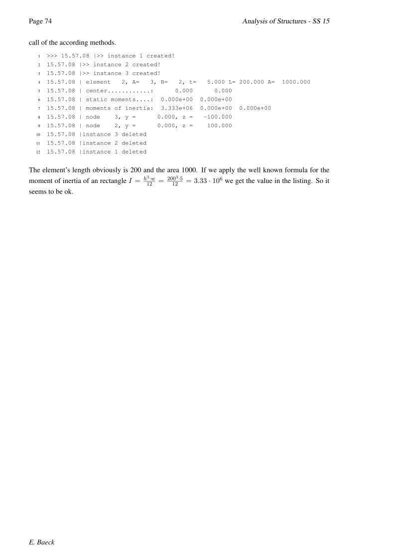
Page 74 Analysis of Structures - SS 15
call of the according methods.
1 >>> 15.57.08 |>> instance 1 created!
2 15.57.08 |>> instance 2 created!
3 15.57.08 |>> instance 3 created!
4 15.57.08 | element 2, A= 3, B= 2, t= 5.000 L= 200.000 A= 1000.000
5 15.57.08 | center............: 0.000 0.000
6 15.57.08 | static moments....: 0.000e+00 0.000e+00
7 15.57.08 | moments of inertia: 3.333e+06 0.000e+00 0.000e+00
8 15.57.08 | node 3, y = 0.000, z = -100.000
9 15.57.08 | node 2, y = 0.000, z = 100.000
10 15.57.08 |instance 3 deleted
11 15.57.08 |instance 2 deleted
12 15.57.08 |instance 1 deleted
The element’s length obviously is 200 and the area 1000. If we apply the well known formula for themoment of inertia of an rectangle I = h3·w
12 = 2003·512 = 3.33 · 106 we get the value in the listing. So it
seems to be ok.
E. Baeck

3.2. PROFILES, THIN WALLED APPROACH Page 75
3.2.6 A General Profile Class
So if we want to develop a software, which is able to calculate the profile’s section properties like it’sarea, moment of inertia and so on, we can consequently split up the problem in general and specificparts. So we start with the data and the functions of a general object. This data is collected in a classwhich we call Base. So if we want to describe a wide range of profile types, then we should think aboutthe profile’s common features. Every profile has a name and therefore this name is a common feature.This common features are collected in a general profile class which is called Profile. If we want tohandle a specific profile type given by a set of parameters like an U-profile ore a tube profile, we collectthe specific type dependent features in the classes UProfile and TubeProfile, which are obviously theparameters describing the profile’s geometry.
The class Profile now contents common profile features. One of them is the profile’s name. Note,if we inherit a class from a base class, we have to call the base class’s constructor method. Everyattribute and every method of the base class is now available. A second feature of the Profile class isthe implementation of the thin walled model. Therefore we introduce an Element container using theAList class. With a specific method we insert an Element instance into the container. To calculate thesection values of the created thin walled model we introduce some methods, which calculate the globalsection values summing up all element values and transforming them into the desired coordinate system.
At least we introduce a little viewing method, which should create a png picture file of the profile andshould optionally start the pylab viewer tool. To be sure, that the environment supports the Tkinterpackage1, which is used by the viewer, we import the package using a try: ... except: handler.At the end of the view method we should close the plot, to avoid a memory effect.
Profile
+ self. name: The profile’s name
+ self. elem: Element container
− self. init (..): constructor
+ self.list(..): List profiles values
+ self.addElement(..): insert a new Element
+ self.getResults(): calculate section values
− self.getPValues(): transform the moment of inertia
− self.pTrans(): principal axis transformation
+ self.view(..): views a profile plot
The class Profile contents allcommon features of a profileespecially the containers for thePoints and Lines of shape modell
The class Profile contents allcommon features of a profileespecially the containers for thePoints and Lines of shape modell
Figure 3.7: The general Profile Class
A U-profile is described within the frame of the TWA by it’s height and width as well as by the thicknessesof it’s web and flange. So we need 4 floats to do this. It’s UML diagram is given in figure 3.8.
1We will see later trying to apply our package Profiles in the frame of the Abaqus scripting, that we will get problems,because the Abaqus environment is not developed with Tkinter.
8.5.2018

Page 76 Analysis of Structures - SS 15
UProfile
+ self. h: height
+ self. w: with
+ self. s: web thickness
+ self. t: flange thickness
− self. init (..): constructor
+ self.list(..): list profiles values
+ self.check(): check input values
+ self.create(..): create thin walled model
The class UProfile contents thespecial features of an U-Profile,i.e. the geometric parameters.The class will be inherit the Pro-file class and will have the featureto create this profile with an Ugeometry.
The class UProfile contents thespecial features of an U-Profile,i.e. the geometric parameters.The class will be inherit the Pro-file class and will have the featureto create this profile with an Ugeometry.
Figure 3.8: The U-Profile Class
A tube-profile is described within the frame of the TWA by it’s diameter and it’s thickness. So we needonly 2 floats to do this. It’s UML diagram is given in figure 3.9.
TubeProfile
+ self. d: diameter
+ self. t: thickness
− self. init (..): constructor
+ self.list(..): list profiles values
+ self.check(): check input values
+ self.create(..): create thin walled model
The class TubeProfile contentsthe special features of a Tube-Profile, especially the geometricparameters
The class TubeProfile contentsthe special features of a Tube-Profile, especially the geometricparameters
Figure 3.9: The Tube-Profile Class
To hold the desired Element instances we implement a slightly modified list class, which shouldwork like an array with a well defined index access (see section 3.2.7). If we would use a standard listclass, we would get problems if we want to insert an object at a position outside the list range. Then astandard list object simply appends this object as a new item at the tail of the list and we would loose thecorrect index position. So we implement a new index save Add method, which checks the list length andif necessary enlarges the list up to the desired index position.
The implementation of the class Profile is given in listing 3.7.
Listing 3.7: Implementation of an Profile-Class
1 # -*- coding: utf-8 -*-
2
3 __author__ = ’baeck’
4 ’’’
5 Profile class to calculate section values
6 with the thinwalled approximation
7 ’’’
8
9 from Base import Base
10 from AList import AList
11
E. Baeck
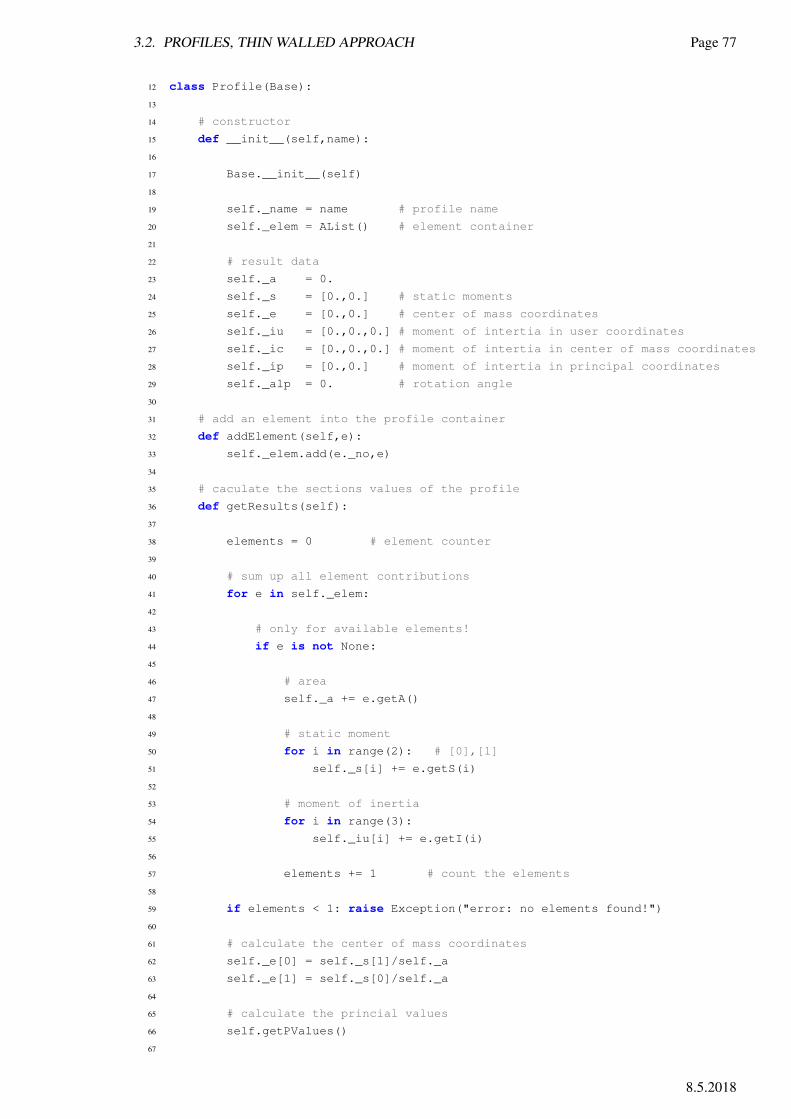
3.2. PROFILES, THIN WALLED APPROACH Page 77
12 class Profile(Base):
13
14 # constructor
15 def __init__(self,name):
16
17 Base.__init__(self)
18
19 self._name = name # profile name
20 self._elem = AList() # element container
21
22 # result data
23 self._a = 0.
24 self._s = [0.,0.] # static moments
25 self._e = [0.,0.] # center of mass coordinates
26 self._iu = [0.,0.,0.] # moment of intertia in user coordinates
27 self._ic = [0.,0.,0.] # moment of intertia in center of mass coordinates
28 self._ip = [0.,0.] # moment of intertia in principal coordinates
29 self._alp = 0. # rotation angle
30
31 # add an element into the profile container
32 def addElement(self,e):
33 self._elem.add(e._no,e)
34
35 # caculate the sections values of the profile
36 def getResults(self):
37
38 elements = 0 # element counter
39
40 # sum up all element contributions
41 for e in self._elem:
42
43 # only for available elements!
44 if e is not None:
45
46 # area
47 self._a += e.getA()
48
49 # static moment
50 for i in range(2): # [0],[1]
51 self._s[i] += e.getS(i)
52
53 # moment of inertia
54 for i in range(3):
55 self._iu[i] += e.getI(i)
56
57 elements += 1 # count the elements
58
59 if elements < 1: raise Exception("error: no elements found!")
60
61 # calculate the center of mass coordinates
62 self._e[0] = self._s[1]/self._a
63 self._e[1] = self._s[0]/self._a
64
65 # calculate the princial values
66 self.getPValues()
67
8.5.2018

Page 78 Analysis of Structures - SS 15
68 return (self._a,self._s,self._ip,self._alp)
69
70 # calculate the principal values
71 # shift and rotate!
72 def getPValues(self):
73 import math
74
75 # shift the moment of inertia into the center of mass cs
76 self._ic[0] = self._iu[0] - self._e[1]*self._e[1]*self._a
77 self._ic[1] = self._iu[1] - self._e[0]*self._e[0]*self._a
78 self._ic[2] = self._iu[2] - self._e[0]*self._e[1]*self._a
79
80 # introduce some helpers
81 idel = self._ic[0] - self._ic[1]
82 isum = self._ic[0] + self._ic[1]
83 isqr = math.sqrt(idel*idel + 4.*self._ic[2]*self._ic[2])
84
85 # calculate the principal values
86 self._ip[0] = 0.5*(isum + isqr)
87 self._ip[1] = 0.5*(isum - isqr)
88
89 # calculate the rotation angle
90 self._alp = 0.5*math.atan2(-2.*self._ic[2],idel)
91
92 # get angle value in degrees
93 self._alp *= 45./math.atan(1.)
94
95 # list the profile’s data
96 def listData(self):
97 self.appendLog("name..................: %s" % self._name)
98 self.appendLog("area..................: %10.2f cmˆ2" % (self._a/1.e2,))
99 self.appendLog("center of mass .......: %10.2f %10.2f cm" % \
100 (self._e[0]/1.e1,self._e[1]/1.e1))
101 self.appendLog("static moments .......: %10.2f %10.2f cmˆ3" % \
102 (self._s[0]/1.e3,self._s[1]/1.e3))
103 self.appendLog("moment of inertia uc: %10.2f %10.2f %10.2f cmˆ4" % \
104 (self._iu[0]/1.e4,self._iu[1]/1.e4,self._iu[2]/1.e4))
105 self.appendLog("moment of inertia cc: %10.2f %10.2f %10.2f cmˆ4" % \
106 (self._ic[0]/1.e4,self._ic[1]/1.e4,self._ic[2]/1.e4))
107 self.appendLog("moment of inertia pc: %10.2f %10.2f cmˆ4" % \
108 (self._ip[0]/1.e4,self._ip[1]/1.e4))
109 self.appendLog("rotation angle : %10.2f " % self._alp)
110
111 # print a picture of the profile geometry
112 def view(self,viewer = True):
113
114 try:
115 import pylab
116 except:
117 self.appendLog("error: pylab not intalled!")
118 return
119
120
121 # list of lines. every element -> a line
122 lines = []
123
E. Baeck
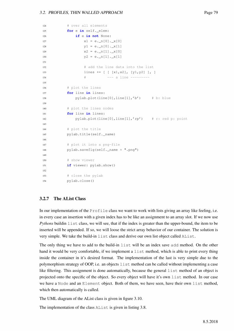
3.2. PROFILES, THIN WALLED APPROACH Page 79
124 # over all elements
125 for e in self._elem:
126 if e is not None:
127 x1 = e._n[0]._x[0]
128 y1 = e._n[0]._x[1]
129 x2 = e._n[1]._x[0]
130 y2 = e._n[1]._x[1]
131
132 # add the line data into the list
133 lines += [ [ [x1,x2], [y1,y2] ], ]
134 # --- a line ---------
135
136 # plot the lines
137 for line in lines:
138 pylab.plot(line[0],line[1],’b’) # b: blue
139
140 # plot the lines nodes
141 for line in lines:
142 pylab.plot(line[0],line[1],’rp’) # r: red p: point
143
144 # plot the title
145 pylab.title(self._name)
146
147 # plot it into a png-file
148 pylab.savefig(self._name + ".png")
149
150 # show viewer
151 if viewer: pylab.show()
152
153 # close the pylab
154 pylab.close()
3.2.7 The AList Class
In our implementation of the Profile class we want to work with lists giving an array like feeling, i.e.in every case an insertion with a given index has to be like an assignment to an array slot. If we now usePythons buildin list class, we will see, that if the index is greater than the upper-bound, the item to beinserted will be appended. If so, we will loose the strict array behavior of our container. The solution isvery simple. We take the build-in list class and derive our own list object called AList.
The only thing we have to add to the build-in list will be an index save add method. On the otherhand it would be very comfortable, if we implement a list method, which is able to print every thinginside the container in it’s desired format. The implementation of the last is very simple due to thepolymorphism strategy of OOP, i.e. an objects list method can be called without implementing a caselike filtering. This assignment is done automatically, because the general list method of an object isprojected onto the specific of the object. So every object will have it’s own list method. In our casewe have a Node and an Element object. Both of them, we have seen, have their own list method,which then automatically is called.
The UML diagram of the AList class is given in figure 3.10.
The implementation of the class AList is given in listing 3.8.
8.5.2018

Page 80 Analysis of Structures - SS 15
Base list Python’s build-inlist containerPython’s build-inlist container
AList
− self. init (..): constructor
+ self.add(..): Add by index
+ self.list(..): print instance’s data
The class AList is based on thepython build-in list class. TheAdd method adds an object with agiven index value.
The class AList is based on thepython build-in list class. TheAdd method adds an object with agiven index value.
Figure 3.10: UML-Diagram for a Array-List Class
Listing 3.8: Implementation of an AList-Class
1 __author__ = ’baeck’
2
3 ’’’
4 extends the python’s buildin class List
5 to get a perfect array feeling
6 ’’’
7
8 from Base import Base
9
10 class AList(Base,list):
11
12 # constructor
13 def __init__(self):
14 Base.__init__(self)
15
16 # add an instance like an array would do
17 # no : index
18 # ojb: object
19 def add(self,no,obj):
20 # check the length
21 ubound = len(self) -1
22
23 if no > ubound:
24 for i in range(ubound+1,no+1):
25 self += [None,]
26
27 # store it!
28 self[no] = obj
29
30 # print the list’s content
31 def list(self):
32 lobj = 0 # counter
33
34 # iterate the container
35 for obj in self:
36
E. Baeck

3.2. PROFILES, THIN WALLED APPROACH Page 81
37 try:
38 obj.list()
39 except:
40 self.appendLog("object %d is unprintable" % lobj)
41 # pass
42
43 lobj += 1
In line 6 we can see, that the AList has two base classes Base and list. The features of both classesare inherited by our new one. Base is used to print and list is used to store the instance pointers.
In line 15 we see the new method add. If the index is less than the list’s length a general list add is done.If not, we first enlarge the list up to the needed index value and then call the standard function. If wedo so, the list also can have wholes inside, i.e. None pointers. So we have to be careful with the arrayaccess.
In line 27 we call the list method of every list index. To avoid crashing we simple make the list accessa save access by putting it into a try-except environment.
The Profile class can be considered as a container class for the Element instances. The cardinality isone and greater. One we would have for a flat steel, two for an L profile and three for a U profile. TheUML diagram is given in figure 3.11.
1 1..*
Base Profile Element
Figure 3.11: Profile’s Element Container
3.2.8 Testing the Profile Class
To test the Profile class we implement a simple main program which creates the points of a TWAbased approximation of the unsymmetric L-profile L 100x50x6. The plates of the L have the length 100and 50 mm. The thickness of the L is 5 mm.
The implementation of the testing environment is given in listing 3.9.
Listing 3.9: Implementation of a Profile-Testing Environment
1 ’’’
2 check the Profile class
3 3
4 | :2
5 :1 |
6 1---2
7 ’’’
8 import Profile
9 reload(Profile)
10
11 from Profile import Profile
12 from Element import Element
8.5.2018
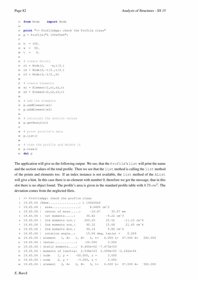
Page 82 Analysis of Structures - SS 15
13 from Node import Node
14
15 print ">> ProfileApp: check the Profile class"
16 p = Profile("L 100x50x6")
17
18 h = 100.
19 w = 50.
20 t = 6.
21
22 # create Noints
23 n1 = Node(1, -w,t/2.)
24 n2 = Node(2,-t/2.,t/2.)
25 n3 = Node(3,-t/2.,h)
26
27 # create elements
28 e1 = Element(1,n1,n2,t)
29 e2 = Element(2,n2,n3,t)
30
31 # add the elements
32 p.addElement(e1)
33 p.addElement(e2)
34
35 # calculate the section values
36 p.getResults()
37
38 # print profile’s data
39 p.list()
40
41 # view the profile and delete it
42 p.view()
43 del p
The application will give us the following output. We see, that the Profile’s list will print the nameand the section values of the total profile. Then we see that the list method is calling the list methodof the points and elements too. If an index instance is not available, the list method of the AListwill give a hint. In this case there is no element with number 0, therefore we get the message, that in thisslot there is no object found. The profile’s area is given in the standard profile table with 8.73 cm2. Thedeviation comes from the neglected filets.
1 >> ProfileApp: check the profile class
2 19.45.04 |Name.................: L 100x50x6
3 19.45.04 | area...............: 8.6400 cmˆ2
4 19.45.04 | center of mass.....: -10.67 35.67 mm
5 19.45.04 | 1st moments.....: 30.82 -9.22 cmˆ3
6 19.45.04 | 2nd moments ucs.: 200.25 25.52 -11.23 cmˆ4
7 19.45.04 | 2nd moments scs.: 90.32 15.68 21.65 cmˆ4
8 19.45.04 | 2nd moments mcs.: 96.14 9.86 cmˆ4
9 19.45.04 | rotation angle..: 15.06 deg, tan(a) = 0.269
10 19.45.04 | element 1, A= 1, B= 2, t= 6.000 L= 47.000 A= 282.000
11 19.45.04 | center............: -26.500 3.000
12 19.45.04 | static moments....: 8.460e+02 -7.473e+03
13 19.45.04 | moments of inertia: 2.538e+03 2.499e+05 -2.242e+04
14 19.45.04 | node 1, y = -50.000, z = 3.000
15 19.45.04 | node 2, y = -3.000, z = 3.000
16 19.45.04 | element 2, A= 2, B= 3, t= 6.000 L= 97.000 A= 582.000
E. Baeck

3.2. PROFILES, THIN WALLED APPROACH Page 83
17 19.45.04 | center............: -3.000 51.500
18 19.45.04 | static moments....: 2.997e+04 -1.746e+03
19 19.45.04 | moments of inertia: 2.000e+06 5.238e+03 -8.992e+04
20 19.45.04 | node 2, y = -3.000, z = 3.000
21 19.45.04 | node 3, y = -3.000, z = 100.000
Figure 3.12: pylab - View of the Profile
Figure 3.12 shows the output of theprofile’s viewmethod. First the pic-ture is created, then a png file is writ-ten from the picture and at the endthe viewer is started.2
2Note, that the viewer of the used version is very sensible for multiple calls. So if you want to restart the program, youshould first close an open viewer instance. If not, the program will hang.
8.5.2018

Page 84 Analysis of Structures - SS 15
3.2.9 The U-Profile Class
Figure 3.13 shows the UML diagram of the UProfile class. The parameters we pass to the classesconstructor are it’s name, the height, the width and the thicknesses of web and flange.
UProfile
+ self. h: height
+ self. w: with
+ self. s: web thickness
+ self. t: flange thickness
− self. init (..): constructor
+ self.list(..): list profiles values
+ self.check(): check input values
+ self.create(..): create thin walled model
The class UProfile contents thespecial features of an U-Profile,i.e. the geometric parameters.The class will be inherit the Pro-file class and will have the featureto create this profile with an Ugeometry.
The class UProfile contents thespecial features of an U-Profile,i.e. the geometric parameters.The class will be inherit the Pro-file class and will have the featureto create this profile with an Ugeometry.
Figure 3.13: The U-Profile Class
A class hierarchy UML diagram is given in figure 3.14.
Base Profile UProfile
Figure 3.14: The U-Profile Class Hierarchy
The implementation of the class UProfile is given in listing 3.10. The method create creates theprofile’s Node and Element instances. Before the geometry data is created the input parameters of theU geometry should be checked. To cancel further activities, the simplest solution is to raise an exceptionto break the execution.
Listing 3.10: Implementation of an UProfile-Class
1 ’’’
2 Implementaion of a UProfile class
3 ’’’
4 from Profile import Profile
5 from Node import Node
6 from Element import Element
7
8 class UProfile(Profile):
9
10 def __init__(self,name,h,w,s,t):
11
12 Profile.__init__(self,name)
13
14 self._h = h # height
15 self._w = w # width
16 self._s = s # web thickness
17 self._t = t # flansch thickness
18
E. Baeck

3.2. PROFILES, THIN WALLED APPROACH Page 85
19 # check input parameters
20 self.check()
21
22 # create the geomtry data
23 self.create()
24
25 # check the input parameters
26 def check(self):
27 dMin = 1.
28
29 # checking the parameters
30 if self._h < dMin:
31 raise Exception("invalid height h: %e" % self._h)
32 if self._w < dMin:
33 raise Exception("invalid width w: %e" % self._w)
34 if self._s < dMin:
35 raise Exception("invalid thickness s: %e" % self._s)
36 if self._t < dMin:
37 raise Exception("invalid thickness t: %e" % self._t)
38
39 # create the datastructure of an u-profile
40 def create(self):
41
42 hs = (self._h - self._t)/2.
43 ws = self._w - self._s/2.
44
45 # create the nodes
46 n1 = Node(1,0., hs)
47 n2 = Node(2,0.,-hs)
48 n3 = Node(3,ws, hs)
49 n4 = Node(4,ws,-hs)
50
51 # create the elements
52 e1 = Element(1,n1,n2,self._s)
53 e2 = Element(2,n1,n3,self._t)
54 e3 = Element(3,n2,n4,self._t)
55
56 # assign the elements
57 self.addElement(e1)
58 self.addElement(e2)
59 self.addElement(e3)
3.2.10 Testing the UProfile Class
To test the UProfile class we implement a simple main program, which passes the name and theparameters of a U-geometry to the UProfile constructor. Then the data of the instance is printed. Inour example we calculate the values of an U80.
8.5.2018

Page 86 Analysis of Structures - SS 15
The implementation of the testing environment is given in listing 3.11.
Listing 3.11: Implementation of a UProfile-Testing Environment
1 ’’’
2 check the UProfile class
3 ’’’
4 import UProfile
5 reload(UProfile)
6
7 from UProfile import UProfile
8
9 print ">> UProfileApp: check the profile class"
10 try:
11 # name h w s t
12 p = UProfile("U80",80,45, 6, 8)
13
14 # calculate the section values
15 p.getResults()
16
17 # print profile’s data
18 p.list()
19
20 # view the profile’s system
21 p.view()
22
23 # delete the instance
24 del p
25 except Exception,e:
26 print "*** error:",e
27
28 print ">> UProfileApp: stop"
The following lines show the output of the test application. The exact value of the U profile’s area is11 cm2. Note that we have to put the constructor call into a try-except frame to catch the exception.
1 >> UProfileApp: check the profile class
2 19.57.13 |Name.................: U80
3 19.57.13 | area...............: 11.0400 cmˆ2
4 19.57.13 | center of mass.....: 12.78 0.00 mm
5 19.57.13 | 1st moments.....: 0.00 14.11 cmˆ3
6 19.57.13 | 2nd moments ucs.: 105.75 39.51 0.00 cmˆ4
7 19.57.13 | 2nd moments scs.: 105.75 21.47 0.00 cmˆ4
8 19.57.13 | 2nd moments mcs.: 105.75 21.47 cmˆ4
9 19.57.13 | rotation angle..: 0.00 deg, tan(a) = 0.000
10 19.57.13 | element 1, A= 1, B= 2, t= 6.000 L= 72.000 A= 432.000
11 19.57.13 | center............: 0.000 0.000
12 19.57.13 | static moments....: 0.000e+00 0.000e+00
13 19.57.13 | moments of inertia: 1.866e+05 0.000e+00 0.000e+00
14 19.57.13 | node 1, y = 0.000, z = 36.000
15 19.57.13 | node 2, y = 0.000, z = -36.000
16 19.57.13 | element 2, A= 1, B= 3, t= 8.000 L= 42.000 A= 336.000
17 19.57.13 | center............: 21.000 36.000
18 19.57.13 | static moments....: 1.210e+04 7.056e+03
19 19.57.13 | moments of inertia: 4.355e+05 1.976e+05 2.540e+05
20 19.57.13 | node 1, y = 0.000, z = 36.000
21 19.57.13 | node 3, y = 42.000, z = 36.000
E. Baeck

3.2. PROFILES, THIN WALLED APPROACH Page 87
22 19.57.13 | element 3, A= 2, B= 4, t= 8.000 L= 42.000 A= 336.000
23 19.57.13 | center............: 21.000 -36.000
24 19.57.13 | static moments....: -1.210e+04 7.056e+03
25 19.57.13 | moments of inertia: 4.355e+05 1.976e+05 -2.540e+05
26 19.57.13 | node 2, y = 0.000, z = -36.000
27 19.57.13 | node 4, y = 42.000, z = -36.000
28 >> UProfileApp: stop
Figure 3.15: pylab - View of the Profile
Figure 5.2 shows the output of theprofile’s viewmethod. First the pic-ture is created, then a png file is writ-ten from the picture and at the endthe viewer is started.
3.2.11 The Profile Package
If we want to develop reusable code, it’s recommended to create a separate file for every class and putthem into a package. A package is a folder with the package’s name and a file called __init__.py.If the __init__.py file is not found within the folder, the folder is not interpreted as a package andthe software components of the package can not be loaded. So we introduce a folder called Profile.To initialize a package we have to create a file named __init__.py in this folder. If the package isloaded, the __init__.py is executed. All our class files we put into this package folder.
Listing 3.12: Initializing the Package
1 # This script is executed only once, if the package is loaded.
2 # So we print a little to show what’s going on
3 print ">> Package ’Profiles’ is loaded"
If we implement a new class within the Profile package, we only have to import the module base, i.e.the file Base.py. From this module we import the class Base. So we can write the import statement asfollows.3
1 from Base import Base # inherit from the Base
If we want to use a class from a package, we have to import it with the following statement.
1 from <package>.<module> import <class> as <locale name / alias name>
3Note, that the file names are case sensitive although you may work on Windows plattform.
8.5.2018

Page 88 Analysis of Structures - SS 15
As an example we use the application for testing a U-profile (see listing 3.11). We move the file on folderup, so that all our used class files are living in the subfolder Profile.4
The implementation of the testing environment using the package Profile is given in listing 3.13.
Listing 3.13: Implementation of a UProfile-Testing Environment using Package Profile
1 ’’’
2 check the UProfile class
3 ’’’
4 import Profile.UProfile # import total module
5 reload(Profile.UProfile) # reload total module
6 # make sure that’s the current
7 from Profile.UProfile import UProfile # import from a package
8 # from here on every thing is the same...
9 print ">> UProfileApp: check the profile class"
10 try:
11 # name h w s t
12 p = UProfile("U80",80,45, 6, 8)
13
14 # print profile’s data
15 p.listData()
16
17 # delete the instance
18 del p
19 except Exception,e:
20 print "*** error:",e
21
22 print ">> UProfileApp: stop"
3.2.12 A Little Profile Database
To implement a simple profile data base for arbitrary profile instances, we can simply use the Pythonbuildin object dict 5 and extend it by inheritance with a specific list method (see figure 3.16). The listiterates the dictionary getting the keys of the stored instances. With the given key we get the instancepointer from the dictionary. Then we can use the mechanism of the polymorphism and call the instancesspecific list method. If there is an error occurring, the try/except error handler will do his job andexecutes the except branch code. So we can avoid program crashing due to invalid ore missing pointers.
The code of the ProfileDB class is given below.
Listing 3.14: Implementation of a Profile-Database, the ProfDB-Class
1 from Base import Base # the ProfDB class should inherit the Base class
2
3 # The ProfileDB class should store arbitray profile objects in
4 # a dictionary. Therefore we inherit from the buildin dict object
5 class ProfileDB(Base,dict):
6
7 def __init__(self):
8 Base.__init__(self) # call the Base constructor
9
4Note, if we do so, we also can move the total folder Profile into Pythons folder Lib/site-packages.5A dictionary is used to store instance pointers with an arbitrary access key.
E. Baeck

3.2. PROFILES, THIN WALLED APPROACH Page 89
ProfileDB
− self. init (..): constructor
+ self.list(..): print instance’s data
The class ProfileDB is based on aa dictionary. Profile instances areare stored like in a database.
The class ProfileDB is based on aa dictionary. Profile instances areare stored like in a database.
dictPython’s build-in dictionary classPython’s build-in dictionary class
Figure 3.16: UML-Diagram of the Profile Database
10 # the List method calls the List method of it’s items
11 # if there is no item, the case is handled with an exception block
12 def list(self):
13 iobj = 0 # initialize the object counter
14 for name in self: # iterate the keys of the dictionary
15 try: # open the try block
16 self[name].list() # try to list an object
17 except: # if not possible log it to the log file
18 self.appendLog(" Error: No profile key %s found, slot %d" % \
19 (name,iobj))
20 iobj += 1 # increment the counter
21
22 # the View method calls the View method of it’s items with a False Flag.
23 # if there is no item, the case is handled with an exception block
24 def view(self):
25 iobj = 0 # initialize the object counter
26 for name in self: # iterate the keys of the dictionary
27 try: # open the try block
28 self[name].View(False) # try to write the png file
29 except: # if not possible log it to the log file
30 self.appendLog(" Error: No profile key %s found, slot %d" % \
31 (name,iobj))
32 iobj += 1 # increment the counter
To check the database class ProfileDB we write a little script, which first creates a ProfileDB instance.Then we create a UProfile instance with the values of the U100. This instance is stored in the dictionaryusing the key of it’s name U100. Then we create a second UProfile instance with the values of the U140and store it as well in the dictionary using it’s name U140 as it’s key. After that we simple call theProfileDB instance method list. The data of the two profiles are listed on the screen and into the log file.After the job is done, we print the png files of our profiles. The code of the testing environment is givenbelow, the resulting png files are shown in figure .
8.5.2018

Page 90 Analysis of Structures - SS 15
Listing 3.15: Implementation of a Testing-Environment for the ProfileDB-Class
1 ’’’
2 This testing example implements a little profile
3 database. Two U-profiles are created and stored in
4 the database. Then the whole content of the database
5 is printed using the AppendLog method of the base class
6 ’’’
7 # package module class
8 from Profile.UProfile import UProfile
9 from Profile.ProfileDB import ProfileDB
10
11
12 # create Profile database
13 db = ProfileDB()
14
15 # create the instance of an U-Profile
16 prof = UProfile("U100",100.,50.,6.0,8.5)
17
18 # and save it into the db
19 db.setDefault("U100",prof)
20
21 # create the instance of an U-Profile
22 prof = UProfile("U140",140.,60.,7.0,10.)
23
24 # and save it into the db
25 db.setDefault("U140",prof)
26
27 # print the content of the db
28 db.list()
29
30 # print png files of the content of the db
31 db.view()
Figure 3.17: Pictures of the Profiles stored in the Database
E. Baeck

Part II
Scripting with Abaqus
91


4
Some Aspects and Introduction
In this chapter we talk about the Abaqus Student Edition Licence 6.10.. A main aspect will be thedevelopment of Python programs, which should automate the creation of FE models and the subsequentcalculation and preprocessing.
4.1 Aspects of the Abaqus GUI
In this chapter we talk about the Abaqus Student Edition Licence 6.10. GUI1.
Figure 4.1 shows the Abaqus GUI. A very important item is the combo box to select the module. Theselected module loads the specific menu items. The left window shows the Abaqus object tree. Thebottom window contents an output window for the output messages and the command window for thePython commands.
Figure 4.1: Abaqus-GUI
1Graphical User Interface is a window driven program which contents all commands in terms of menu items, buttons, boxesand so on which are commonly called widgets.
93
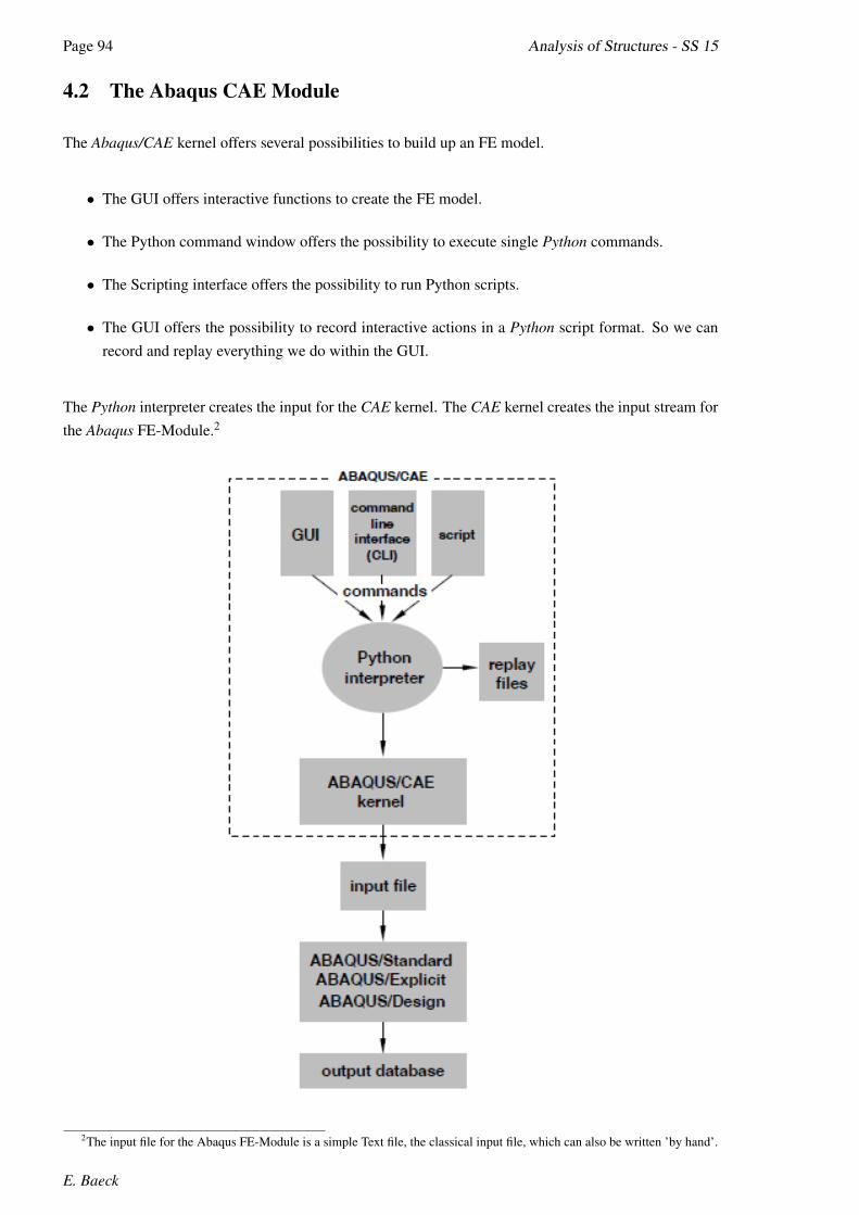
Page 94 Analysis of Structures - SS 15
4.2 The Abaqus CAE Module
The Abaqus/CAE kernel offers several possibilities to build up an FE model.
• The GUI offers interactive functions to create the FE model.
• The Python command window offers the possibility to execute single Python commands.
• The Scripting interface offers the possibility to run Python scripts.
• The GUI offers the possibility to record interactive actions in a Python script format. So we canrecord and replay everything we do within the GUI.
The Python interpreter creates the input for the CAE kernel. The CAE kernel creates the input stream forthe Abaqus FE-Module.2
2The input file for the Abaqus FE-Module is a simple Text file, the classical input file, which can also be written ’by hand’.
E. Baeck

4.3. A MODELING CHAIN Page 95
4.3 A Modeling Chain
Create Database
Module SketchDraw a sketch
Module PartCreate a part andassign the sketch
Module PropertyCreate a properties, ma-terials and sections, as-
sign them to sketch lines
Module AssemblyCreate an instance and
assign the part to it
Module StepCreate a step as
container for a load case
Module LoadCreate loads andboundary condi-
tion within the step
Module MeshSet Seeds, elementsper length select andassign element typemesh the instance
Module JobCreate a Job and submit
Module PostprocessingVisualization
and Evaluation
Figure 4.2:Modeling Chain Diagram
Figure 4.2 shows how to create a Finite Element model in Abaqus/CAE. Itis not possible to create elements and nodes directly. Element and nodes areonly created by the mesh generator, which works an the geometric objects,which are created drawing a sketch.
The only FE model parameter, which are created directly, are the materialproperties and the section values. This properties are created within themodule Property. The properties are then assigned to the geometric objects(lines, areas and volumes).
After having created a sketch the sketch has to be assigned to a part. If nopart exists, a part hast to be created. The properties (materials and sectiondata) are assigned to the sketches’ geometric objects.
To create a mesh, an instance is needed, so an instance has to be created.The part with the sketch are assigned to the instance for later meshing.
Loadcases are modeled in terms of load steps. So a new step has to be cre-ated as a container for loads and boundary conditions. Loads and bound-aries are assigned to the geometric objects of the sketch which were as-signed to a part before.
To create the mesh, the mesh’s control parameters should be configured andthe element types are to be assigned. Then the instance can be meshed.
After the mesh is created, the complete model can be assigned to a job. Tocalculate the results the job has to be submitted.
8.5.2018

Page 96 Analysis of Structures - SS 15
4.4 A little interactive Warm Up Example
x
yFx
Fy
Lx
Ly
Figure 4.3: 3 Trusses
In section 4.3 we have discussed the Abaqus modeling chain. Fol-lowing this outlines the subsequent example based on [5] shows howto create and calculate a simple 3 truss system with a concentratedforce. We use the following parameters.
• Lx horizontal length 1000 mm
• Ly vertical length 1500 mm
• Fx horizontal force -100 kN
• Fy vertical force -100 kN
4.4.1 Create a Database
Create Model Database
File/Set Working Directory (setup the desired work folder if necessary)
4.4.2 Create a Sketch
Module: Sketch
Sketch => Create => Name: ’Truss-Example’ => Continue
Add=> Point
=> enter coordinates (0,0), (1000,0), (1000,1500), (0,1500)
Add => Line => Connected Line
=> select (0,0) node with mouse, then (1000,0) node,
right click => Cancel
Add => Line
=> Connected Line
=> select (0,0) node with mouse, then (1000,1500) node,
right click => Cancel
Add => Line
=> Connected Line
=> select (0,0) node with mouse, then (0,1500) node,
right click => Cancel
=> Done
4.4.3 Create a Part
Module: Part
Part => Create => Name: ’Part-1’,=> select 2D Planar, Deformable, Wire
=> Continue
Add => Sketch => select ’Truss-Example’ => Done => Done
E. Baeck

4.4. A LITTLE INTERACTIVE WARM UP EXAMPLE Page 97
4.4.4 Create and Assign Properties
Module: Property
Material => Create => Name: ’Steel’, Mechanical, Elasticity, Elastic
=> set Young’s modulus = 210000, Poisson’s ratio = 0.3 => OK
Section => Create => Name: ’Truss-Section’, Beam, Truss => Continue
=> set Material: ’Material-1’,
Cross-sectional area: 2
Assign Section => select all elements by dragging mouse => Done
=> ’Truss-Section’ => OK => Done
4.4.5 Create the Instance, Assign the Part
Module: Assembly
Instance => Create => ’Part-1’ => Independent (mesh on instance) => OK
4.4.6 Create a Load Step
Module: Step
Step => Create => Name: ’Step-1’, Initial, Static, General => Continue
=> accept default settings
=> OK
4.4.7 Create Loads and Boundary Conditions
Module: Load
Load => Create => Name: ’Step-1’, Step: ’Step 1’, Mechanical,
Concentrated Force => Continue => select node at (0,0) => Done
=> set CF1: -10000 set CF2: -10000 => OK
BC => Create => Name: ’BC-1’, Step: ’Step-1’, Mechanical,
Displacement/Rotation => Continue
=> select nodes at (1000,0), (1000,1500) and (0,1500) using SHIFT key
to select multiple nodes => Done => set U1: 0 and U2: 0
4.4.8 Create the Mesh
Module: Mesh
Seed => Edge by Number => select entire truss by dragging mouse
=> Done => Number of elements along edges: 1 => press Enter => Done
Mesh => Element Type => select entire truss by dragging mouse => Done
=> Element Library: Standard,
Geometric Order: Linear: Family: Truss => OK => Done
Mesh => Instance => OK to mesh the part Instance: Yes
8.5.2018

Page 98 Analysis of Structures - SS 15
4.4.9 Create a Job and Submit
Module: Job
Job => Create => Name: Job-1, Model: Model-1 => Continue
=> Job Type: Full analysis, Run Mode: Background,
Submit Time: Immediately => OK
Job => Submit => ’Job-1’
Job => Manager => Results (enters Module: Visualization)
E. Baeck

5
Scripts and Examples
In this chapter we implement to example scripts, to discuss the automation in Abaqus using the Pythonscript language.
1. 3 TrussesThe first script gives the implementation of the interactive example, a little 3 trusses system withone concentrated load. The calculation is performed automatically for a linear analysis.
2. U ProfileThe second script gives the implementation of the automated model creation of U Profile using thethin-walled approach (see also section 3.2 and B.1). The calculation is performed automaticallyfor a linear analysis and a buckling analysis.
5.1 3 Trusses Script
Within this section the implementation of a script is shown, which automates the example of section4.4. With the change of the parameter’s values, every system can be calculated with the execution of thescript.
Creating the calculation model we follow our outlines discussed in section 4.3. To avoid problems withexisting project files, we first delete an old database, if exist. Then we set the work directory by the useof Python’s standard chdir function.1
To get the Python code for the necessary steps, we can simple run the macro recorder and record theinteractive actions. If you do this, then it’s recommended to save the macro file into the work directoryand not into the home directory. The recorded macros are saved into the file abaqusMacros.py.Note, that the work directory will be set, if the script is executed.
Within the script code the following steps are numbered in the same way.
(1) Create a modelThe model is member of the global mdb class. We have to specify the name and the type of themodel. The reference to the created model is saved into the variable myModel for further usage.
1Note, that on Windows-Systems a path contents backslashes, which in Python are used as escape characters. Therefore ifa backslash is used, we have to duplicate it.
99
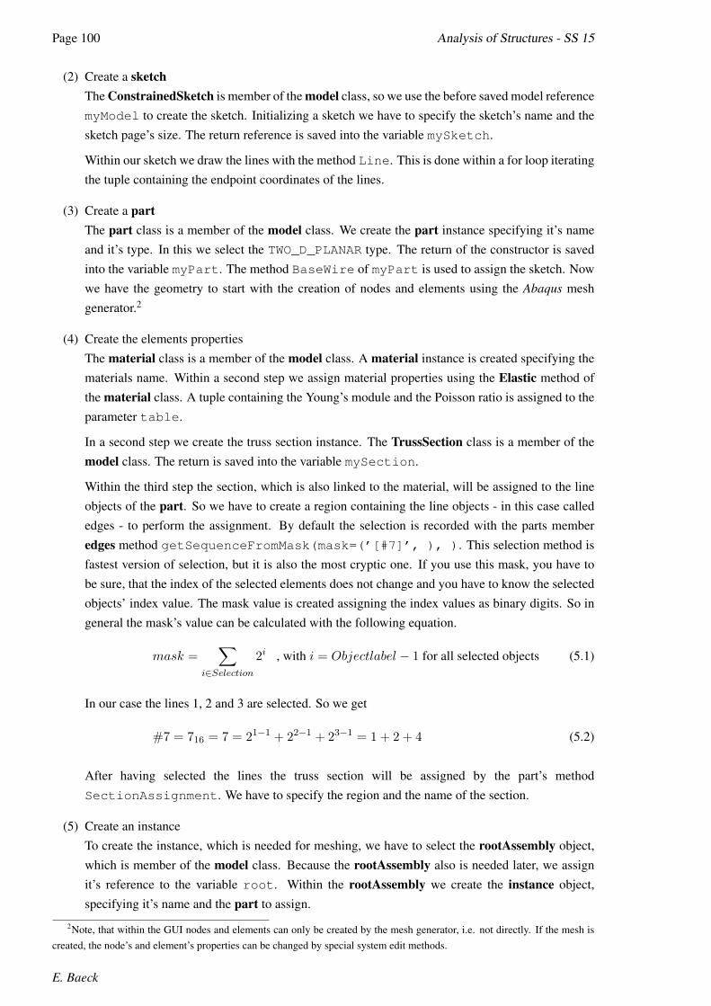
Page 100 Analysis of Structures - SS 15
(2) Create a sketchThe ConstrainedSketch is member of the model class, so we use the before saved model referencemyModel to create the sketch. Initializing a sketch we have to specify the sketch’s name and thesketch page’s size. The return reference is saved into the variable mySketch.
Within our sketch we draw the lines with the method Line. This is done within a for loop iteratingthe tuple containing the endpoint coordinates of the lines.
(3) Create a partThe part class is a member of the model class. We create the part instance specifying it’s nameand it’s type. In this we select the TWO_D_PLANAR type. The return of the constructor is savedinto the variable myPart. The method BaseWire of myPart is used to assign the sketch. Nowwe have the geometry to start with the creation of nodes and elements using the Abaqus meshgenerator.2
(4) Create the elements propertiesThe material class is a member of the model class. A material instance is created specifying thematerials name. Within a second step we assign material properties using the Elastic method ofthe material class. A tuple containing the Young’s module and the Poisson ratio is assigned to theparameter table.
In a second step we create the truss section instance. The TrussSection class is a member of themodel class. The return is saved into the variable mySection.
Within the third step the section, which is also linked to the material, will be assigned to the lineobjects of the part. So we have to create a region containing the line objects - in this case callededges - to perform the assignment. By default the selection is recorded with the parts memberedges method getSequenceFromMask(mask=(’[#7]’, ), ). This selection method isfastest version of selection, but it is also the most cryptic one. If you use this mask, you have tobe sure, that the index of the selected elements does not change and you have to know the selectedobjects’ index value. The mask value is created assigning the index values as binary digits. So ingeneral the mask’s value can be calculated with the following equation.
mask =∑
i∈Selection2i , with i = Objectlabel − 1 for all selected objects (5.1)
In our case the lines 1, 2 and 3 are selected. So we get
#7 = 716 = 7 = 21−1 + 22−1 + 23−1 = 1 + 2 + 4 (5.2)
After having selected the lines the truss section will be assigned by the part’s methodSectionAssignment. We have to specify the region and the name of the section.
(5) Create an instanceTo create the instance, which is needed for meshing, we have to select the rootAssembly object,which is member of the model class. Because the rootAssembly also is needed later, we assignit’s reference to the variable root. Within the rootAssembly we create the instance object,specifying it’s name and the part to assign.
2Note, that within the GUI nodes and elements can only be created by the mesh generator, i.e. not directly. If the mesh iscreated, the node’s and element’s properties can be changed by special system edit methods.
E. Baeck

5.1. 3 TRUSSES SCRIPT Page 101
(6) Create loads and boundary conditionsFirst we should create a StaticStep class, which is a member of the modul class. The StaticStepclass is a container for loads and boundary conditions.
To create a concentrated load, which is a points load, we have to select first some points, which arecalled vertices in Abaqus. The vertices container is a member of the instance class. Vertices alsocan be selected with the getSequenceFromMask method, if the label number of the points areknown. The class methode regionToolset.region converts a set of vertices into a region.The class ConcentratedForce is a member of the model class. We have to specify the loads name.We have to assign the load to a step and a region and have to set up the load values.
To create boundary conditions we select vertices as well and convert them into a region. Then theDisplacementBC object, a member of the instance class has to be created like the concentratedforces specifying it’s name and assigning it to a load step.
(7) Create the meshThe mesh will be created on the geometric data, in this case the lines of the sketch. So we haveto set up the seeds of the lines, the number of elements, which should be created by the meshgenerator. Like in the case of the section assignment we select all lines using the edges containerof the part object. With #7 we set the mask for our 3 lines. To set the numbers of elements,we apply the method seedEdgeByNumber of the part class passing the selected edges and thenumber of elements to create, in this case one.
Within a second step we select the element type to use in our model with the method elemType ofthe class mesh. We select from the standard element library the truss element with the code T2D2.Then the selected element type is assigned to all elements using the method setElementTypeof the part class. As parameters we pass a region, which is created with the mask #7 for all edgesand with an tuple of selected element types.
Within an ultimate step we simple call the method generateMesh of the part class.
Now the mesh is created with all it’s properties and with the method setValues of the standardviewport instance, which is a member of the session class, we can view the mesh passing thepart instance as displayedObject parameter. If no viewport is explicitly created, the standardviewport is called Viewport: 1.
(8) Create the job and submitWe set up the jobname and create the job using the standard parameter values. In this case thejob is executed immediately after submission. The return value of the creation step is saved into avariable for later usage. After the creation of the job, the job is submitted with the job classes’ themethod submit. To automate the analysis of the results two features are available.
– synchronous analysisIn this case the script halts for completion of the calculation. This can be obtained by theusage of the job classes’ method waitForCompletion. The next commands of the scriptare executed after the calculation is completed.
– asynchronous analysisIn this case the script does not halt for completion and the next instructions are executedimmediately. To automate the analysis of the results we have to set up a call back function.This function is executed automatically after the calculation is done.
8.5.2018
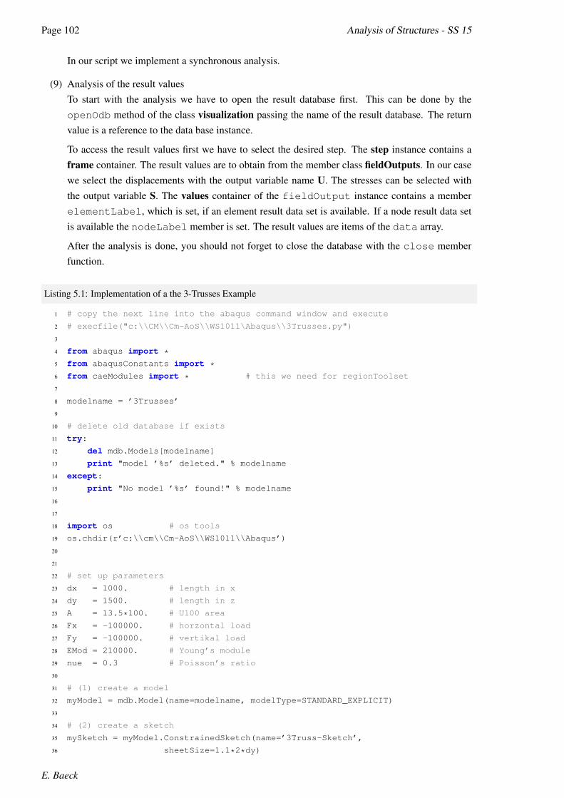
Page 102 Analysis of Structures - SS 15
In our script we implement a synchronous analysis.
(9) Analysis of the result valuesTo start with the analysis we have to open the result database first. This can be done by theopenOdb method of the class visualization passing the name of the result database. The returnvalue is a reference to the data base instance.
To access the result values first we have to select the desired step. The step instance contains aframe container. The result values are to obtain from the member class fieldOutputs. In our casewe select the displacements with the output variable name U. The stresses can be selected withthe output variable S. The values container of the fieldOutput instance contains a memberelementLabel, which is set, if an element result data set is available. If a node result data setis available the nodeLabel member is set. The result values are items of the data array.
After the analysis is done, you should not forget to close the database with the close memberfunction.
Listing 5.1: Implementation of a the 3-Trusses Example
1 # copy the next line into the abaqus command window and execute
2 # execfile("c:\\CM\\Cm-AoS\\WS1011\Abaqus\\3Trusses.py")
3
4 from abaqus import *5 from abaqusConstants import *6 from caeModules import * # this we need for regionToolset
7
8 modelname = ’3Trusses’
9
10 # delete old database if exists
11 try:
12 del mdb.Models[modelname]
13 print "model ’%s’ deleted." % modelname
14 except:
15 print "No model ’%s’ found!" % modelname
16
17
18 import os # os tools
19 os.chdir(r’c:\\cm\\Cm-AoS\\WS1011\\Abaqus’)
20
21
22 # set up parameters
23 dx = 1000. # length in x
24 dy = 1500. # length in z
25 A = 13.5*100. # U100 area
26 Fx = -100000. # horzontal load
27 Fy = -100000. # vertikal load
28 EMod = 210000. # Young’s module
29 nue = 0.3 # Poisson’s ratio
30
31 # (1) create a model
32 myModel = mdb.Model(name=modelname, modelType=STANDARD_EXPLICIT)
33
34 # (2) create a sketch
35 mySketch = myModel.ConstrainedSketch(name=’3Truss-Sketch’,
36 sheetSize=1.1*2*dy)
E. Baeck

5.1. 3 TRUSSES SCRIPT Page 103
37
38 # - create tuple with coordinates
39 xyPoint = ( (0,0), (dx,0), (dx,dy), (0,dy) )
40 # - iterate the tuple and draw lines
41 for i in range(1,len(xyPoint)):
42 mySketch.Line(point1=xyPoint[0], point2=xyPoint[i])
43
44 # (3) create part
45 myPart = myModel.Part(name=’Trusse-Part-1’,
46 dimensionality=TWO_D_PLANAR, type=DEFORMABLE_BODY)
47
48 # - assign the sketch
49 myPart.BaseWire(sketch=mySketch)
50
51 # (4) set up properties
52 # - create material for steel
53 mySteel = myModel.Material(name = ’Steel’)
54 mySteel.Elastic(table=( (EMod,nue), ))
55
56 # - create truss section
57 mySection = myModel.TrussSection(name=’Truss-Section’, area=A,
58 material=’Steel’)
59
60 # - assign the section to all lines
61 alledges = myPart.edges
62 edges = alledges.getSequenceFromMask(mask=(’[#7 ]’, ), )
63 region = regionToolset.Region(edges=edges)
64 myPart.SectionAssignment(region=region, sectionName=’Truss-Section’, offset=0.0,
65 offsetType=MIDDLE_SURFACE, offsetField=’’,
66 thicknessAssignment=FROM_SECTION)
67
68 # (5) create an instance
69 root = myModel.rootAssembly
70 myInst = root.Instance(name=’Trusses-Instance’, part=myPart, dependent=ON)
71
72 # (6) create a load step
73 myModel.StaticStep(name=’First Step’, previous=’Initial’,
74 description=’Static Load Step’)
75
76 # - create loads for the loadstep
77 v1 = myInst.vertices
78 verts1 = v1.getSequenceFromMask(mask=(’[#2 ]’, ), )
79 region = regionToolset.Region(vertices=verts1)
80 myModel.ConcentratedForce(name=’Load-1’,
81 createStepName=’First Step’, region=region, cf1=Fx, cf2=Fy,
82 distributionType=UNIFORM, field=’’, localCsys=None)
83
84 # - create boundary conditions for the loadstep
85 verts1 = v1.getSequenceFromMask(mask=(’[#d ]’, ), )
86 region = regionToolset.Region(vertices=verts1)
87 myModel.DisplacementBC(name=’BC-1’,
88 createStepName=’First Step’, region=region, u1=0.0, u2=0.0, ur3=UNSET,
89 amplitude=UNSET, fixed=OFF, distributionType=UNIFORM, fieldName=’’,
90 localCsys=None)
91
92 # (7) create mesh
8.5.2018

Page 104 Analysis of Structures - SS 15
93 # - number of elments / line
94 e = myPart.edges
95 pickedEdges = e.getSequenceFromMask(mask=(’[#7 ]’, ), )
96 myPart.seedEdgeByNumber(edges=pickedEdges, number=1, constraint=FINER)
97
98 # - set up the element type
99 elemType1 = mesh.ElemType(elemCode=T2D2, elemLibrary=STANDARD)
100 e = myPart.edges
101 edges = e.getSequenceFromMask(mask=(’[#7 ]’, ), )
102 Region=(edges, )
103 myPart.setElementType(regions=Region, elemTypes=(elemType1, ))
104
105 # - create the mesh
106 myPart.generateMesh()
107
108 # - show the mesh
109 session.viewports[’Viewport: 1’].setValues(displayedObject=myPart)
110
111 # (8) create a job and submit it
112 jobname = modelname+’-Job-1’
113 myJob = mdb.Job(name=jobname, model=modelname,
114 description=’Calculation of the 3 Trusses System’, type=ANALYSIS,
115 atTime=None, waitMinutes=0, waitHours=0, queue=None, memory=50,
116 memoryUnits=PERCENTAGE, getMemoryFromAnalysis=True,
117 explicitPrecision=SINGLE, nodalOutputPrecision=SINGLE, echoPrint=OFF,
118 modelPrint=OFF, contactPrint=OFF, historyPrint=OFF, userSubroutine=’’,
119 scratch=’’)
120 myJob.submit(consistencyChecking=OFF)
121
122 # - note: wait for completion, if the result values should be read form DB
123 myJob.waitForCompletion()
124
125
126 # (9) analysis of results
127 # - open the database: odb file
128 myOdb = visualization.openOdb(jobname+’.odb’)
129
130 # - read data from the last frame
131 frame = myOdb.steps[’First Step’].frames[-1]
132
133 # - printing the displacements
134 data = frame.fieldOutputs[’U’]
135 n = len(data.values)
136 print "%d Result records" % n
137 print ’--no ---ux----- ---uy----’
138 for value in data.values:
139 print "%4d %10.5f %10.5f" % (value.nodeLabel,value.data[0],value.data[1])
140
141 # - printing the stresses
142 data = frame.fieldOutputs[’S’]
143 n = len(data.values)
144 print "%d Result records" % n
145 print ’--no --S11-----’
146 for value in data.values:
147 print "%4d %10.5f" % (value.elementLabel,value.data[0])
148
E. Baeck

5.1. 3 TRUSSES SCRIPT Page 105
149 # close the database
150 myOdb.close()
Figure 5.2 shows the system with it’s loads and boundary condition (see figure 4.3 too). All points arefixed but not lower left. Here we see the applied point loads in down and left direction.
Figure 5.1: Loads and Boundary Conditions
Figure 5.2 shows the magnitude of displacement on the deformed truss structure.
Figure 5.2: Magnitude of Displacement
8.5.2018

Page 106 Analysis of Structures - SS 15
5.2 U-Girder Script
Figure 5.3: U Profile
The goal of our next example is, to create a mesh from a 2 dimensional sketch ofan U geometry by extrusion. Figure 5.2 shows an U profile with it’s parameters[6]. The U profile geometry is used to create a FE model of a single span girder,shown in figure 5.4. The girder has a length of L and will be loaded with a lineload q. The boundary conditions should be set according to the simple singlegirder system.
The model of the U profile is created step by step according to the modeling chaindiagram (figure 4.2). The created mesh is shown in figure 5.9. Figure ?? showsthe load onto the upper flange of the girder. The girder is supported on both endsat the lower flange’s edges.
Additional point support is needed to avoid longitudinal and transversal move-ments as well as rigid body rotations. If we would not do this, it would be likewalking on perfect ice. We may glide in both horizontal directions and may rotate around the verticalaxis without any resistivity. So the stiffness matrix of the girder would be singular without the suppres-sion of this degrees of freedom (dof ). So we have to fix three dof s which will suppress this rigid bodymoves on an arbitrary point in the system. After the calculation is done we will see, whether the choicewas ok, if the reaction forces on this fixed dof s are numerically vanishing.
5.2.1 System and Automated Analysis
q
L
Figure 5.4: Single SpanGirder
Figure 5.4 shows the single span girder in terms of a simple beam. Theload q is distributed constantly on the girder length L. One end of thegirder is supported hinged and the other side is supported with a rollersupport.
The following steps of analysis should be done automated by the script.
• According to the calculation switches the script automatically should be able to do a linear staticcalculation, a buckling analysis or a frequency analysis;
• for a calculation with loads, the script should check automatically the load balancing, i.e. it shouldcheck whether the applied load will be totally seen as reaction forces;
• the script should find all nodes along a given longitudinal system fiber;
• along this fiber the maximal displacement should be evaluated;
• pictures of the relevant results should be created in terms of png-files.
E. Baeck
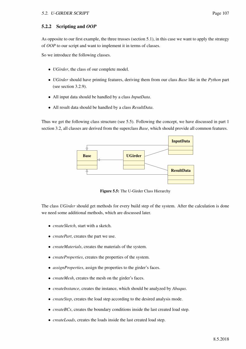
5.2. U-GIRDER SCRIPT Page 107
5.2.2 Scripting and OOP
As opposite to our first example, the three trusses (section 5.1), in this case we want to apply the strategyof OOP to our script and want to implement it in terms of classes.
So we introduce the following classes.
• UGirder, the class of our complete model.
• UGirder should have printing features, deriving them from our class Base like in the Python part(see section 3.2.9).
• All input data should be handled by a class InputData.
• All result data should be handled by a class ResultData.
Thus we get the following class structure (see 5.5). Following the concept, we have discussed in part 1section 3.2, all classes are derived from the superclass Base, which should provide all common features.
Base UGirder
InputData
ResultData
Figure 5.5: The U-Girder Class Hierarchy
The class UGirder should get methods for every build step of the system. After the calculation is donewe need some additional methods, which are discussed later.
• createSketch, start with a sketch.
• createPart, creates the part we use.
• createMaterials, creates the materials of the system.
• createProperties, creates the properties of the system.
• assignProperties, assign the properties to the girder’s faces.
• createMesh, creates the mesh on the girder’s faces.
• createInstance, creates the instance, which should be analyzed by Abaqus.
• createStep, creates the load step according to the desired analysis mode.
• createBCs, creates the boundary conditions inside the last created load step.
• createLoads, creates the loads inside the last created load step.
8.5.2018

Page 108 Analysis of Structures - SS 15
5.2.3 Class InputData
Figure 5.6 shows the UML class diagram of the InputData class. This class is used to assemble, checkand work up the girder’s parameters.
InputData
+ self.h: profile’s height
+ self.w: profile’s width
+ self.t: profile’s flange thickness
+ self.s: profile’s web thickness
+ self.len: girder’s length
+ self.load: load to apply on girder’s top face
+ ... some attributes more
+ self. init (..): constructor
+ self.setHelpers(..): create helper data
+ self.check(..): check the input parameter
+ self.read(..): read parameters from an input file
Only the most importantattributes are shown in thediagram to get a compactpicture. All attributes aregiven in the following ta-ble.
Only the most importantattributes are shown in thediagram to get a compactpicture. All attributes aregiven in the following ta-ble.
Figure 5.6: UML-Diagram of the InputData Class
Attribute Dimension Comment
prjName − project’s name
h mm profile’s height
w mm profile’s width
t mm profile’s flange thickness
s mm profile’s web thickness
len m girder’s length
load kN applied load
ymod N/mm2 Young’s module
nue 1 Poisson ratio
nue kg/mm3 mass density (used for frequency analysis)
maxElement 1 maximal allowed element and node number
webSeed 1 element number along the the web edge
flangeSeed 1 element number along the the flange edge
stepType − specifies the calculation type (static, stability, dynamic)
Besides the parameters discussed in the table above, there are some other attributes in the class, whichare used to prepare or initialize the parameter set for the calculation. This attributes are explained insidethe code.
E. Baeck
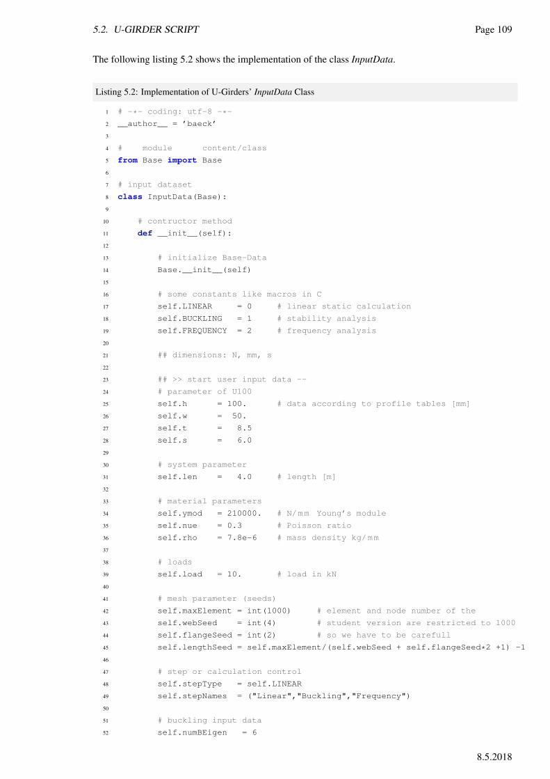
5.2. U-GIRDER SCRIPT Page 109
The following listing 5.2 shows the implementation of the class InputData.
Listing 5.2: Implementation of U-Girders’ InputData Class
1 # -*- coding: utf-8 -*-
2 __author__ = ’baeck’
3
4 # module content/class
5 from Base import Base
6
7 # input dataset
8 class InputData(Base):
9
10 # contructor method
11 def __init__(self):
12
13 # initialize Base-Data
14 Base.__init__(self)
15
16 # some constants like macros in C
17 self.LINEAR = 0 # linear static calculation
18 self.BUCKLING = 1 # stability analysis
19 self.FREQUENCY = 2 # frequency analysis
20
21 ## dimensions: N, mm, s
22
23 ## >> start user input data --
24 # parameter of U100
25 self.h = 100. # data according to profile tables [mm]
26 self.w = 50.
27 self.t = 8.5
28 self.s = 6.0
29
30 # system parameter
31 self.len = 4.0 # length [m]
32
33 # material parameters
34 self.ymod = 210000. # N/mm Young’s module
35 self.nue = 0.3 # Poisson ratio
36 self.rho = 7.8e-6 # mass density kg/mm
37
38 # loads
39 self.load = 10. # load in kN
40
41 # mesh parameter (seeds)
42 self.maxElement = int(1000) # element and node number of the
43 self.webSeed = int(4) # student version are restricted to 1000
44 self.flangeSeed = int(2) # so we have to be carefull
45 self.lengthSeed = self.maxElement/(self.webSeed + self.flangeSeed*2 +1) -1
46
47 # step or calculation control
48 self.stepType = self.LINEAR
49 self.stepNames = ("Linear","Buckling","Frequency")
50
51 # buckling input data
52 self.numBEigen = 6
8.5.2018
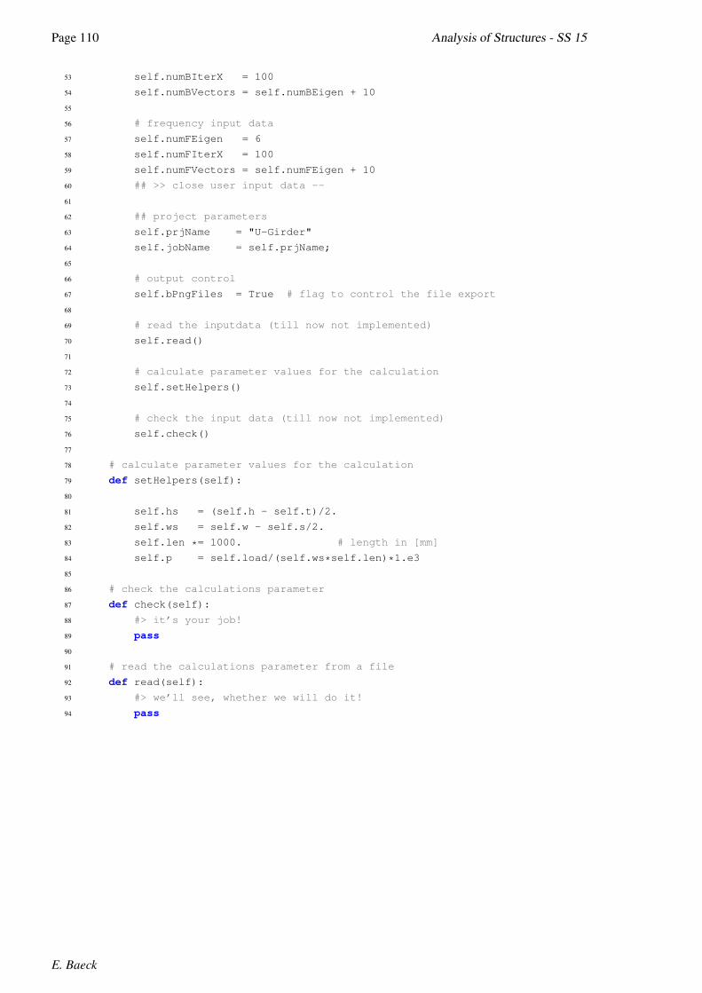
Page 110 Analysis of Structures - SS 15
53 self.numBIterX = 100
54 self.numBVectors = self.numBEigen + 10
55
56 # frequency input data
57 self.numFEigen = 6
58 self.numFIterX = 100
59 self.numFVectors = self.numFEigen + 10
60 ## >> close user input data --
61
62 ## project parameters
63 self.prjName = "U-Girder"
64 self.jobName = self.prjName;
65
66 # output control
67 self.bPngFiles = True # flag to control the file export
68
69 # read the inputdata (till now not implemented)
70 self.read()
71
72 # calculate parameter values for the calculation
73 self.setHelpers()
74
75 # check the input data (till now not implemented)
76 self.check()
77
78 # calculate parameter values for the calculation
79 def setHelpers(self):
80
81 self.hs = (self.h - self.t)/2.
82 self.ws = self.w - self.s/2.
83 self.len *= 1000. # length in [mm]
84 self.p = self.load/(self.ws*self.len)*1.e3
85
86 # check the calculations parameter
87 def check(self):
88 #> it’s your job!
89 pass
90
91 # read the calculations parameter from a file
92 def read(self):
93 #> we’ll see, whether we will do it!
94 pass
E. Baeck

5.2. U-GIRDER SCRIPT Page 111
5.2.4 Class ResultData
Figure 5.7 shows the UML class diagram of the ResultData class. This class is used to hold the calculatedresult data.
ResultData
+ self.nodePos: node data of stiff fiber
+ self.nodeRFo: reaction forces
+ self.nodeDis: node displacements
+ self.sumRFo: sum of reaction forces to check load balancing
+ self. init (..): contructor
+ self.getMaxDisp(..): calculate the maximal fiber displacement
The data containers we usehere are dictionaries, whichare using the node’s key askey value.
The data containers we usehere are dictionaries, whichare using the node’s key askey value.
Figure 5.7: UML-Diagram of the ResultData Class
To get the maximal vertical displacement of a very stiff girder fiber to fade out the cross displacement, wehave to select the fiber’s nodes. This node data is stored in the dictionarry nodePos. After the calculationis done, we can search for the maximal vertical displacement in the subspace of the fiber nodes.
The following listing 5.3 shows the implementation of the class ResultData.
Listing 5.3: Implementation of U-Girders’ ResultData Class
1 # -*- coding: utf-8 -*-
2 __author__ = ’baeck’
3
4 ’’’
5 container for result data
6 ’’’
7 from math import fabs
8 from Base import Base
9
10 class ResultData(Base):
11
12 # constructor
13 def __init__(self):
14 self.nodePos = {} # to store the node coordinates and it’s label
15 self.nodeRFo = {} # to store the reaction forces
16 self.nodeDis = {} # to store the node displacements
17 self.sumRFo = [0.,0.,0.] # sum vector of the reaction forces
18
19 # calculate the maximum displacement along the center line
20 def getMaxDisp(self):
21 max = 0.
22 for label in self.nodePos:
23 disp = self.nodeDis[label]
24 if fabs(disp[1]) > max: max = fabs(disp[1])
25 return max
8.5.2018
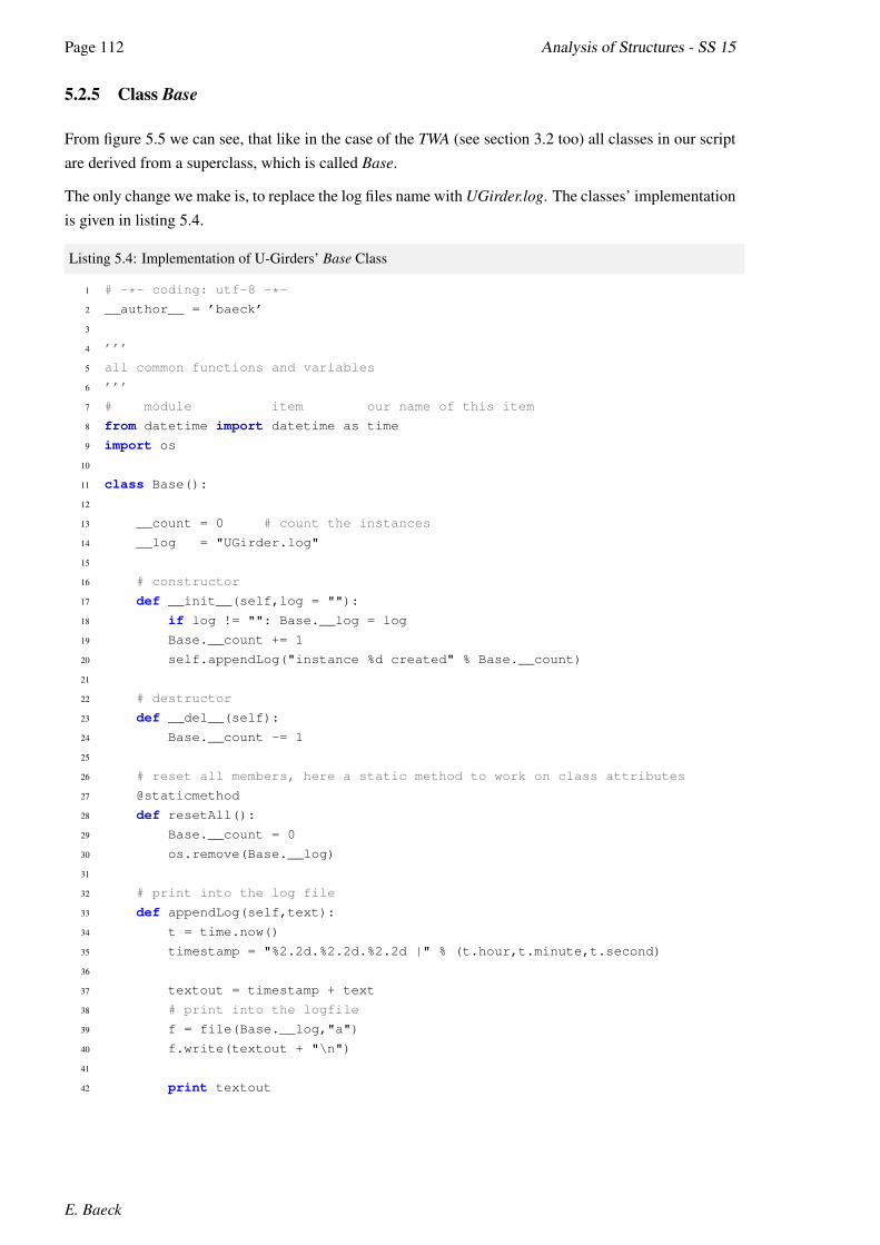
Page 112 Analysis of Structures - SS 15
5.2.5 Class Base
From figure 5.5 we can see, that like in the case of the TWA (see section 3.2 too) all classes in our scriptare derived from a superclass, which is called Base.
The only change we make is, to replace the log files name with UGirder.log. The classes’ implementationis given in listing 5.4.
Listing 5.4: Implementation of U-Girders’ Base Class
1 # -*- coding: utf-8 -*-
2 __author__ = ’baeck’
3
4 ’’’
5 all common functions and variables
6 ’’’
7 # module item our name of this item
8 from datetime import datetime as time
9 import os
10
11 class Base():
12
13 __count = 0 # count the instances
14 __log = "UGirder.log"
15
16 # constructor
17 def __init__(self,log = ""):
18 if log != "": Base.__log = log
19 Base.__count += 1
20 self.appendLog("instance %d created" % Base.__count)
21
22 # destructor
23 def __del__(self):
24 Base.__count -= 1
25
26 # reset all members, here a static method to work on class attributes
27 @staticmethod
28 def resetAll():
29 Base.__count = 0
30 os.remove(Base.__log)
31
32 # print into the log file
33 def appendLog(self,text):
34 t = time.now()
35 timestamp = "%2.2d.%2.2d.%2.2d |" % (t.hour,t.minute,t.second)
36
37 textout = timestamp + text
38 # print into the logfile
39 f = file(Base.__log,"a")
40 f.write(textout + "\n")
41
42 print textout
E. Baeck

5.2. U-GIRDER SCRIPT Page 113
5.2.6 Class UGirder
The UGirder class will be implemented to organize, calculate and analyze the data. The class’ UMLdiagram is shown in figure 5.8.
UGirder
+ self.input: InputData object
+ self.result: ResultData object
+ self.model: Abaqus model
+ self.part: Abaqus part
+ self.material: Abaqus material
+ self.property: Abaqus property
+ self.instance: Abaqus instance
+ self.odb: Abaqus object database
+ self.viewport: Abaqus viewport
+ ... some attributes more
+ self. init (..): constructor
+ self.createSystem(..): create the entire calculation model
+ self.doCalculation(..): starts the solver
Only the most importantattributes are shown in thediagram to get a compactpicture.
Only the most importantattributes are shown in thediagram to get a compactpicture.
Figure 5.8: UML-Diagram of the UGirder Class
The class’ constructor creates an InputData and a ResultData object. To be sure, that all modules arecompiled before execution, i.e. a kind of rebuild, we have to reload this modules. This is only working,if we load them as entire module (see section A.1 too).
Further methods are implemented to add feature by feature to our U-Girder system. All this steps aredone within the method createSystem.
The fist part of the class’ listing 5.5 shows all methods, to create the geometric system and its mesh. Themesh we can see in figure 5.9.
Listing 5.5: Implementation of U-Girders’ Main Class UGirder Class, Part System
1 # -*- coding: utf-8 -*-
2 __author__ = ’baeck’
3
4 ’’’
5 the girder’s main class
6 ’’’
7 # for testing only, to be sure, that every modul will be compiled
8 import Base
9 reload(Base)
10 import InputData
11 reload(InputData)
12 import ResultData
13 reload(ResultData)
14
15 # UGirder imports
16 from Base import Base
8.5.2018

Page 114 Analysis of Structures - SS 15
17 from InputData import InputData
18 from ResultData import ResultData
19 from math import sqrt
20
21 # all abaqus imports
22 from abaqus import *23 from caeModules import *24 from abaqusConstants import *25
26 # the UGirder class
27 class UGirder(Base):
28
29 # constructor
30 def __init__(self):
31 Base.__init__(self)
32 Base.resetAll()
33
34 # references to Abaqus objects
35 self.input = InputData()
36 self.result = ResultData()
37 self.model = None
38 self.sketch = None
39 self.part = None
40 self.materials = []
41 self.properties = []
42 self.instance = None
43 self.odb = None
44 self.viewport = None
45 self.selectFlange = None
46 self.selectWeb = None
47
48 # creates all used objects to create the FEM model
49 def createSystem(self):
50 self.createModel()
51 self.createPart()
52 self.createMaterials()
53 self.createProperties()
54 self.assignProperties()
55 self.createMesh()
56 self.getFiberNodes()
57 self.createInstance()
58
59 # creates the model instance
60 def createModel(self):
61 self.appendLog("create model...")
62 try:
63 del mdb.models[self.input.prjName]
64 except:
65 pass
66 self.model = mdb.Model(name=self.input.prjName)
67
68 # creates a part from a sketch
69 def createPart(self):
70 self.appendLog("create a part from a sketch...")
71
72 # do a little abbreviation
E. Baeck
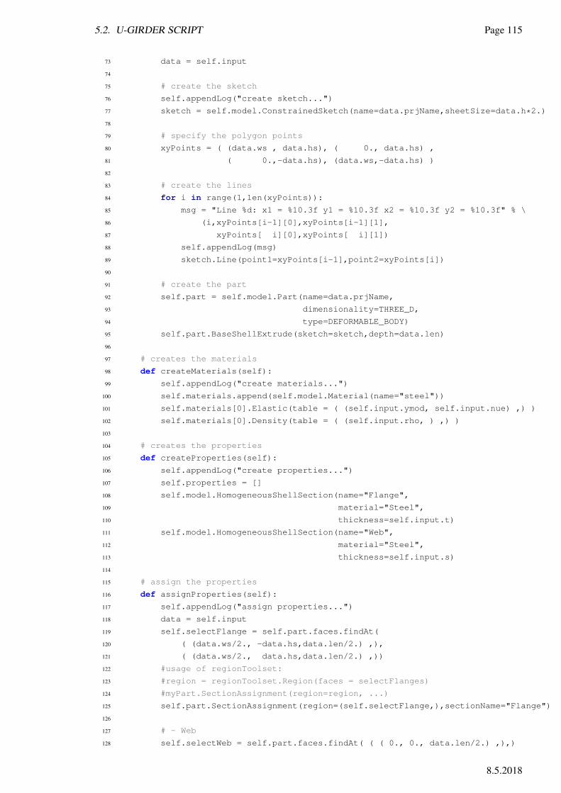
5.2. U-GIRDER SCRIPT Page 115
73 data = self.input
74
75 # create the sketch
76 self.appendLog("create sketch...")
77 sketch = self.model.ConstrainedSketch(name=data.prjName,sheetSize=data.h*2.)
78
79 # specify the polygon points
80 xyPoints = ( (data.ws , data.hs), ( 0., data.hs) ,
81 ( 0.,-data.hs), (data.ws,-data.hs) )
82
83 # create the lines
84 for i in range(1,len(xyPoints)):
85 msg = "Line %d: x1 = %10.3f y1 = %10.3f x2 = %10.3f y2 = %10.3f" % \
86 (i,xyPoints[i-1][0],xyPoints[i-1][1],
87 xyPoints[ i][0],xyPoints[ i][1])
88 self.appendLog(msg)
89 sketch.Line(point1=xyPoints[i-1],point2=xyPoints[i])
90
91 # create the part
92 self.part = self.model.Part(name=data.prjName,
93 dimensionality=THREE_D,
94 type=DEFORMABLE_BODY)
95 self.part.BaseShellExtrude(sketch=sketch,depth=data.len)
96
97 # creates the materials
98 def createMaterials(self):
99 self.appendLog("create materials...")
100 self.materials.append(self.model.Material(name="steel"))
101 self.materials[0].Elastic(table = ( (self.input.ymod, self.input.nue) ,) )
102 self.materials[0].Density(table = ( (self.input.rho, ) ,) )
103
104 # creates the properties
105 def createProperties(self):
106 self.appendLog("create properties...")
107 self.properties = []
108 self.model.HomogeneousShellSection(name="Flange",
109 material="Steel",
110 thickness=self.input.t)
111 self.model.HomogeneousShellSection(name="Web",
112 material="Steel",
113 thickness=self.input.s)
114
115 # assign the properties
116 def assignProperties(self):
117 self.appendLog("assign properties...")
118 data = self.input
119 self.selectFlange = self.part.faces.findAt(
120 ( (data.ws/2., -data.hs,data.len/2.) ,),
121 ( (data.ws/2., data.hs,data.len/2.) ,))
122 #usage of regionToolset:
123 #region = regionToolset.Region(faces = selectFlanges)
124 #myPart.SectionAssignment(region=region, ...)
125 self.part.SectionAssignment(region=(self.selectFlange,),sectionName="Flange")
126
127 # - Web
128 self.selectWeb = self.part.faces.findAt( ( ( 0., 0., data.len/2.) ,),)
8.5.2018

Page 116 Analysis of Structures - SS 15
129 self.part.SectionAssignment(region=(self.selectWeb,),sectionName="Web")
130
131 # creates the mesh
132 def createMesh(self):
133 self.appendLog("generate mesh...")
134 data = self.input
135 # - assign element type: S4R
136 elemType = mesh.ElemType(elemCode = S4R)
137 self.part.setElementType(regions=(self.selectFlange,self.selectWeb),
138 elemTypes = (elemType,))
139
140 # - assign seeds
141 # o flange
142 select = self.part.edges.findAt( ( (data.ws/2., data.hs, 0.), ),
143 ( (data.ws/2.,-data.hs, 0.), ),
144 ( (data.ws/2., data.hs, data.len), ),
145 ( (data.ws/2.,-data.hs, data.len), ),)
146 self.part.seedEdgeByNumber(edges=select,number=data.flangeSeed)
147
148 # o web
149 select = self.part.edges.findAt( ( (0.,0., 0.), ),
150 ( (0.,0., data.len), ),)
151 self.part.seedEdgeByNumber(edges=select,number=data.webSeed)
152
153 # o length direction
154 select = self.part.edges.findAt( ( (data.ws, data.hs, data.len/2.), ),
155 ( ( 0., data.hs, data.len/2.), ),
156 ( ( 0.,-data.hs, data.len/2.), ),
157 ( (data.ws,-data.hs, data.len/2.), ),)
158 self.part.seedEdgeByNumber(edges=select,number=data.lengthSeed)
159
160 # generate mesh
161 self.part.generateMesh()
162
163 # searching for fiber nodes, i.e nodes on the center line
164 def getFiberNodes(self):
165 self.appendLog("find nodes on center fiber...")
166
167 # iterate the container (list: the data is given)
168 for node in self.part.nodes:
169
170 # calculate the distance of the node from the centerline
171 # precision = 1 mm
172 if (sqrt(node.coordinates[0]**2 + node.coordinates[1]**2) < 1.):
173 self.result.nodePos[node.label] = node.coordinates
174
175 self.appendLog("%d elements created." % len(self.part.elements))
176 self.appendLog("%d nodes created." % len(self.part.nodes))
177 self.appendLog("%d nodes on the center line." % len(self.result.nodePos))
178 # print node coordinates on center line
179 # iterate the container (dictionary: -> the key is given)
180 self.appendLog("--no ---------x ---------y ---------z")
181 for label in self.result.nodePos:
182 node = self.result.nodePos[label]
183 self.appendLog("%4d %10.2f %10.2f %10.2f" % \
184 (label,node[0],node[1],node[2]))
E. Baeck

5.2. U-GIRDER SCRIPT Page 117
185
186 # create instance
187 def createInstance(self):
188 self.appendLog("create instance...")
189 self.instance = self.model.rootAssembly.Instance(name=self.input.prjName,
190 part=self.part,
191 dependent=ON)
Figure 5.9: U Girder’s Mesh
To be able to do an independent calculation for the linear static, the stability and the frequency analysis,we first delete an existing load step called Step-1 and then we create the desired type of load step. If wedo this, we easily can run the calculation of all load steps within one calculation loop.
Listing 5.6: Implementation of U-Girders’ Main Class UGirder Class, Part Loads
1
2 # create step
3 def createStep(self,type):
4 self.appendLog("create step of type ’%s’..." % self.input.stepNames[type])
5 self.input.stepType = type
6 # first we have to delete an old created step, to clear the momory
7 if len(self.model.steps) > 1: del self.model.steps["Step-1"]
8 # then we create the new one
9 # create a linear static step with it’s data
10 if type == self.input.LINEAR:
11 self.model.StaticStep(name="Step-1",previous="Initial")
12 self.createBCs(type)
13 self.createLoads(type)
14
15 # create a buckling step
16 elif type == self.input.BUCKLING:
17 self.model.BuckleStep(name="Step-1",
18 previous="Initial",
19 numEigen = self.input.numBEigen,
20 maxIterations = self.input.numBIterX,
21 vectors = self.input.numBVectors)
22 self.createBCs(type)
23 self.createLoads(type)
8.5.2018

Page 118 Analysis of Structures - SS 15
24
25 # create a frequency step
26 elif type == self.input.FREQUENCY:
27 self.model.FrequencyStep(name="Step-1",
28 previous="Initial",
29 eigensolver=SUBSPACE,
30 numEigen = self.input.numFEigen,
31 maxIterations = self.input.numFIterX,
32 vectors = self.input.numFVectors)
33 self.createBCs(type)
34
35 # create BC for the U-girder
36 # stepIndex.: step index
37 def createBCs(self,stepIndex):
38 data = self.input
39 self.appendLog("create boudary conditions...")
40 select = self.instance.edges.findAt( ( (data.ws/2.,data.hs, 0.),),
41 ( (data.ws/2.,data.hs,data.len),),)
42 self.model.DisplacementBC(name="vertical line BCs",
43 createStepName="Step-1",
44 region=(select,),
45 u2=0.0)
46
47 select = self.instance.vertices.findAt( ( (0.,data.hs,0.), ),)
48 self.model.DisplacementBC(name="rigid body mode BCs",
49 createStepName="Step-1",
50 region=(select,),
51 u1=0.0,u3=0.0,ur2=0.0)
52
53 # create loads on the top face of the U girder
54 # stepIndex.: step index
55 def createLoads(self,stepIndex):
56 data = self.input
57 self.appendLog("create loads...")
58 select = self.instance.faces.findAt( ( (data.ws/2.,-data.hs, data.len/2.), ),)
59 region = regionToolset.Region(side1Faces=select)
60 self.model.Pressure(name="flange pressure",
61 createStepName="Step-1",
62 region=region,
63 magnitude=data.p)
Figure 5.10 shows the girder with it’s loads and the boundary conditions after the creation of the stepsLinear Static and Buckling.
Listing 5.7: Implementation of U-Girders’ Main Class UGirder Class, Part Job
1
2 # submit and run the job
3 def runJob(self):
4 self.input.jobName = (self.input.prjName + "-%d") % self.input.stepType
5 self.appendLog("create job %s" % self.input.jobName)
6 job = mdb.Job(name=self.input.jobName,model=self.input.prjName)
7
8 self.input.appendLog("submit job %s" % self.input.jobName)
9 job.submit()
10 job.waitForCompletion()
E. Baeck
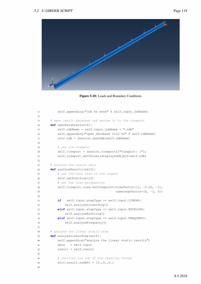
5.2. U-GIRDER SCRIPT Page 119
Figure 5.10: Loads and Boundary Conditions
11 self.appendLog("job %s done" % self.input.jobName)
12
13 # open result database und assign it to the viewport
14 def openDatabase(self):
15 self.odbName = self.input.jobName + ".odb"
16 self.appendLog("open database file %s" % self.odbName)
17 self.odb = session.openOdb(self.odbName)
18
19 # set the viewport
20 self.viewport = session.viewports["Viewport: 1"];
21 self.viewport.setValues(displayedObject=self.odb)
22
23 # analyze the result data
24 def analyzeResults(self):
25 # set the font size of the legend
26 self.setFontSize(12)
27 # set the view perspective
28 self.viewport.view.setViewpoint(viewVector=(1, -0.25, -1),
29 cameraUpVector=(0, -1, 0))
30
31 if self.input.stepType == self.input.LINEAR:
32 self.analyzeLinearStep()
33 elif self.input.stepType == self.input.BUCKLING:
34 self.analyzeBuckling()
35 elif self.input.stepType == self.input.FREQUENCY:
36 self.analyzeFrequency()
37
38 # analyze the linear static step
39 def analyzeLinearStep(self):
40 self.appendLog("analyze the linear static results")
41 data = self.input
42 result = self.result
43
44 # calculte the sum of the reaction forces
45 self.result.sumRFo = [0.,0.,0.]
46
8.5.2018

Page 120 Analysis of Structures - SS 15
47 # - select results
48 # |the last frame
49 frame = self.odb.steps["Step-1"].frames[-1]
50
51 # - select the reaction forces
52 rfo = frame.fieldOutputs[’RF’]
53 # - over all nodes
54 for value in rfo.values:
55 # filter nodes with vanishing RFs
56 if (sqrt( value.data[0]**2
57 + value.data[1]**2
58 + value.data[2]**2 ) > 1.e-10):
59 result.nodeRFo[value.nodeLabel] = value.data
60 for i in range(3): result.sumRFo[i] += value.data[i]
61
62 self.appendLog("sum of the reaction forces: %12.3e %12.3e %12.3e" % tuple(result.sumRFo))
63 error = (data.load*1.e3 + result.sumRFo[1])/(data.load*1.e3)*100.
64 self.appendLog("error.....................: %12.3f %%" % error)
65
66 # iterate and print the RF container (dictionary: -> the key is given)
67 self.appendLog("--no ---------RFx ---------RFy ---------RFz")
68 for label in result.nodeRFo:
69 nodeRF = result.nodeRFo[label]
70 self.appendLog("%4d %12.3e %12.3e %12.3e" % \
71 (label,nodeRF[0],nodeRF[1],nodeRF[2]))
72
73 # - select the node displacements
74 dis = frame.fieldOutputs[’U’]
75 # - over all nodes
76 for value in dis.values:
77 result.nodeDis[value.nodeLabel] = value.data
78
79 self.appendLog("maxium center displacement: %12.3e mm" % result.getMaxDisp())
80
81 # optionally create png-Files
82 if data.bPngFiles:
83
84 varList = ("U1","U2","U3")
85 for var in varList:
86 # plot into the viewport
87 self.viewport.odbDisplay.setPrimaryVariable(
88 variableLabel=’U’,
89 outputPosition=NODAL,
90 refinement=(COMPONENT,var))
91
92 # in colour on the system faces
93 self.viewport.odbDisplay.display.setValues(plotState=(CONTOURS_ON_DEF,))
94 self.viewport.view.fitView()
95
96 # print the image into a file
97 pngFile = data.prjName + "-" + data.stepNames[0] + "-" +var
98 self.printPngFile(pngFile)
99
100 # analyze the buckling step
101 def analyzeBuckling(self):
102 self.appendLog("analyze the buckling step")
E. Baeck

5.2. U-GIRDER SCRIPT Page 121
103 data = self.input
104 result = self.result
105
106 # over all eigenforms
107 for i in range(data.numBEigen):
108
109 # plot into the viewport
110 self.viewport.odbDisplay.setPrimaryVariable(
111 variableLabel=’U’,
112 outputPosition=NODAL,
113 refinement=(INVARIANT,’Magnitude’))
114
115 self.viewport.odbDisplay.display.setValues(plotState=(CONTOURS_ON_DEF,))
116 self.viewport.odbDisplay.setFrame(step="Step-1", frame=i+1)
117 self.viewport.view.fitView()
118
119 pngFile = data.prjName + "-" + data.stepNames[1] + ("-E%2.2d" % (i+1,))
120 self.printPngFile(pngFile)
121
122 # analyze the frequency step
123 def analyzeFrequency(self):
124 self.appendLog("analyze the frequency step")
125 data = self.input
126 result = self.result
127
128 # over all eigenforms
129 for i in range(data.numFEigen):
130
131 # plot into the viewport
132 self.viewport.odbDisplay.setPrimaryVariable(
133 variableLabel=’U’,
134 outputPosition=NODAL,
135 refinement=(INVARIANT,’Magnitude’))
136
137 self.viewport.odbDisplay.display.setValues(plotState=(CONTOURS_ON_DEF,))
138 self.viewport.odbDisplay.setFrame(step="Step-1", frame=i+1)
139 self.viewport.view.fitView()
140
141 pngFile = data.prjName + "-" + data.stepNames[2] + ("-E%2.2d" % (i+1,))
142 self.printPngFile(pngFile)
143
144 # set the fontsize
145 # - size....: font size in [pt]
146 def setFontSize(self,size):
147 fsize = int(size*10)
148 self.viewport.viewportAnnotationOptions.setValues(
149 triadFont=’-*-verdana-medium-r-normal-*-*-%d-*-*-p-*-*-*’ % fsize,
150 legendFont=’-*-verdana-medium-r-normal-*-*-%d-*-*-p-*-*-*’ % fsize,
151 titleFont=’-*-verdana-medium-r-normal-*-*-%d-*-*-p-*-*-*’ % fsize,
152 stateFont=’-*-verdana-medium-r-normal-*-*-%d-*-*-p-*-*-*’ % fsize)
153
154 # print the viewports content into a png file
155 # - pngFile...: file name
156 # - myViewport: data
157 def printPngFile(self,pngFile):
158 session.printOptions.setValues(vpBackground=ON)
8.5.2018

Page 122 Analysis of Structures - SS 15
159 session.printToFile(fileName=pngFile, format=PNG,
160 canvasObjects=(self.viewport,))
5.2.7 Run the UGirder Code
If we organize the girder code using classes the main program to run it will be very lightweight (seelisting 5.8). After setting up the work directory, where we will find the created files, we create the meshof the system. After this we run a loop over all implemented load steps and run the linear static, thebuckling analysis and the frequency analysis.
After the calculation is done the figures are drawn automatically and stored into png files.
Listing 5.8: Implementation a Main Code for U-Girders to Automate the Calculation
1 __author__ = ’baeck’
2
3 ’’’
4 we can start the script using the followning command:
5 execfile(r’[path]\mainUGirder.py’)
6 execfile(r’c:\unidue\CM\Cm-AoS\AOS-BookOfExamples\Py\Code\Abaqus\UGirder\mainUGirder.py’)
7 ’’’
8
9 # set the workdirectory
10 import os
11 os.chdir(r’c:\unidue\CM\Cm-AoS\AOS-BookOfExamples\Py\Code\Abaqus\UGirder’)
12
13 # for testing only
14 import UGirder
15 reload(UGirder)
16
17 # import UGirder and it’s friends
18 from UGirder import UGirder
19
20 # create the geometric system, the mesh
21 sys = UGirder()
22 sys.createSystem()
23
24 # create steps, run job and analyse
25 for i in range(3):
26 sys.createStep(i)
27 sys.runJob()
28 sys.openDatabase()
29 sys.analyzeResults()
E. Baeck

5.2. U-GIRDER SCRIPT Page 123
5.2.7.1 Results of the Linear Static Step
Figure 5.11 shows the resulting displacements in 1(x), 2(y) and 3(z) direction of a linear analysis.
Figure 5.11: Displacement in 1,2 and 3 Direction of a Linear Analysis
8.5.2018

Page 124 Analysis of Structures - SS 15
5.2.7.2 Results of the Buckling Step
Figure 5.12 shows the buckling modes 1 uto 3.
Figure 5.12: Buckling Modes 1 to 3
E. Baeck

5.2. U-GIRDER SCRIPT Page 125
Figure 5.13 shows the buckling modes 4 uto 6.
Figure 5.13: Buckling Modes 4 to 6
8.5.2018

Page 126 Analysis of Structures - SS 15
5.2.7.3 Results of the Frequency Step
Figure 5.14 shows the dynamic modes 1 uto 3.
Figure 5.14: Dynamic Modes 1 to 3
E. Baeck

5.2. U-GIRDER SCRIPT Page 127
Figure 5.15 shows the dynamic modes 4 uto 6.
Figure 5.15: Dynamic Modes 4 to 6
8.5.2018

Page 128 Analysis of Structures - SS 15
E. Baeck
Part III
Appendix
129

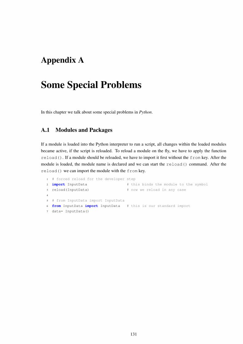
Appendix A
Some Special Problems
In this chapter we talk about some special problems in Python.
A.1 Modules and Packages
If a module is loaded into the Python interpreter to run a script, all changes within the loaded modulesbecame active, if the script is reloaded. To reload a module on the fly, we have to apply the functionreload(). If a module should be reloaded, we have to import it first without the from key. After themodule is loaded, the module name is declared and we can start the reload() command. After thereload() we can import the module with the from key.
1 # forced reload for the developer step
2 import InputData # this binds the module to the symbol
3 reload(InputData) # now we reload in any case
4
5 # from InputData import InputData
6 from InputData import InputData # this is our standard import
7 data= InputData()
131

Page 132 Analysis of Structures - SS 15
E. Baeck
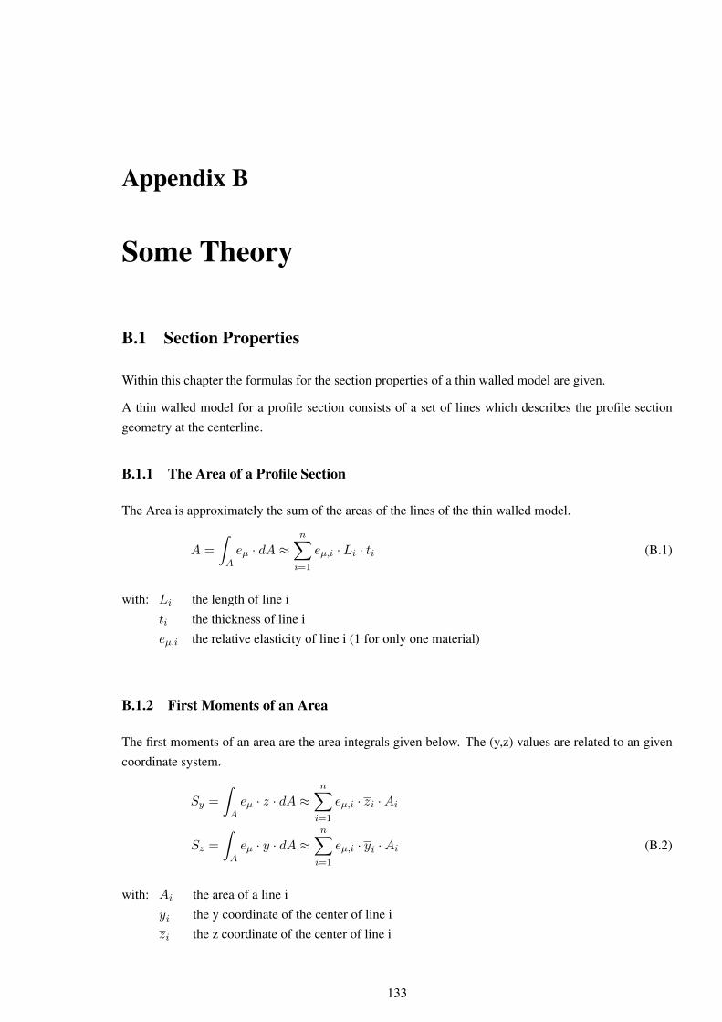
Appendix B
Some Theory
B.1 Section Properties
Within this chapter the formulas for the section properties of a thin walled model are given.
A thin walled model for a profile section consists of a set of lines which describes the profile sectiongeometry at the centerline.
B.1.1 The Area of a Profile Section
The Area is approximately the sum of the areas of the lines of the thin walled model.
A =
∫Aeµ · dA ≈
n∑i=1
eµ,i · Li · ti (B.1)
with: Li the length of line iti the thickness of line ieµ,i the relative elasticity of line i (1 for only one material)
B.1.2 First Moments of an Area
The first moments of an area are the area integrals given below. The (y,z) values are related to an givencoordinate system.
Sy =
∫Aeµ · z · dA ≈
n∑i=1
eµ,i · zi ·Ai
Sz =
∫Aeµ · y · dA ≈
n∑i=1
eµ,i · yi ·Ai (B.2)
with: Ai the area of a line iyi the y coordinate of the center of line izi the z coordinate of the center of line i
133
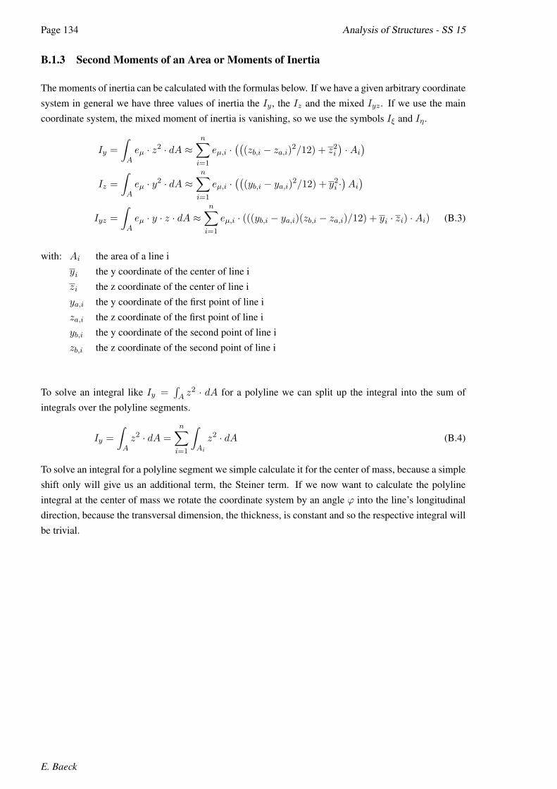
Page 134 Analysis of Structures - SS 15
B.1.3 Second Moments of an Area or Moments of Inertia
The moments of inertia can be calculated with the formulas below. If we have a given arbitrary coordinatesystem in general we have three values of inertia the Iy, the Iz and the mixed Iyz . If we use the maincoordinate system, the mixed moment of inertia is vanishing, so we use the symbols Iξ and Iη.
Iy =
∫Aeµ · z2 · dA ≈
n∑i=1
eµ,i ·(((zb,i − za,i)
2/12) + z2i)·Ai
)Iz =
∫Aeµ · y2 · dA ≈
n∑i=1
eµ,i ·(((yb,i − ya,i)
2/12) + y2i ·)Ai
)Iyz =
∫Aeµ · y · z · dA ≈
n∑i=1
eµ,i · (((yb,i − ya,i)(zb,i − za,i)/12) + yi · zi) ·Ai) (B.3)
with: Ai the area of a line iyi the y coordinate of the center of line izi the z coordinate of the center of line iya,i the y coordinate of the first point of line iza,i the z coordinate of the first point of line iyb,i the y coordinate of the second point of line izb,i the z coordinate of the second point of line i
To solve an integral like Iy =∫A z2 · dA for a polyline we can split up the integral into the sum of
integrals over the polyline segments.
Iy =
∫Az2 · dA =
n∑i=1
∫Ai
z2 · dA (B.4)
To solve an integral for a polyline segment we simple calculate it for the center of mass, because a simpleshift only will give us an additional term, the Steiner term. If we now want to calculate the polylineintegral at the center of mass we rotate the coordinate system by an angle ϕ into the line’s longitudinaldirection, because the transversal dimension, the thickness, is constant and so the respective integral willbe trivial.
E. Baeck

B.1. SECTION PROPERTIES Page 135
Thus we make the following substitution.
(y, z) ⇒ (η, ξ) (B.5)
z = ξ/cos(ϕ) (B.6)
With this substitution we will get the following integral.
Iy,i =
∫ η=+t
η=−t
∫ ξ=+L/2
ξ=−L/2
ξ2
cos(ϕ)2· dη · dξ
= t ·∫ ξ=+L/2
ξ=−L/2
ξ2
cos(ϕ)2· dξ
= t · ξ3
3· 1
cos(ϕ)2
∣∣∣∣ξ=+L/2
ξ=−L/2
= t · L3
12· 1
cos(ϕ)2
=(zb,i − za,i)
2
12·Ai with t · L = Ai (B.7)
B.1.4 Center of Mass
The coordinates of the center of mass are calculated with the arithmetic mean. Because the numerator ofthe arithmetic mean is identical with the first moment of the area (see section B.1.2) and the denominatoris identical with the area of the profile, which is calculated in section B.1.1 we can use this values.
yc =
∫A y · dA∫A dA
=Sz
A
zc =
∫A z · dA∫A dA
=Sy
A(B.8)
B.1.5 Moments of Inertia with Respect to the Center of Mass
If we know the center of mass coordinates given in section B.1.4 we can calculate the moments of inertiawith respect to the center of mass using Steiner’s Theorem as follows.
Iy,c = Iy − z2c ·A
Iz,c = Iz − y2c ·A
Iyz,c = Iyz − yc · zc ·A (B.9)
8.5.2018

Page 136 Analysis of Structures - SS 15
B.1.6 Main Axis Transformation
To get the moments of inertia Iη and Iξ we have to transform the moments of inertia into the maincoordinate system. Using this coordinate system the mixed moment of inertia is vanishing.
The main axis transformation is given with equation B.10.1
Idel = Iy,c − Iz,c
Isum = Iy,c + Iz,c
Isqr =√
I2Del + 4 · I2yz,c
ϕ =1
2· arctan(−2 · Iyz,c
Idel)
Iη =1
2· (Isum + Isqr)
Iξ =1
2· (Isum − Isqr) (B.10)
1The rotation angle ϕ should be shifted into the intervall [−π/2...+ π/2]. To avoid a zero division calculating the rotationangle ϕ a special version of the atan function should be used, which is able to handle the pole problem. In Python like in C thisfunction is called atan2(x, y), which calculates the atan(x
y).
E. Baeck

Appendix C
Some Python IDEs
C.1 The Aptana - IDE
There are lot of IDEs available for the development of Python software. Most of them are commercial.One very nice IDE especially for large development projects with a lot of Python files is called Aptana.Apatana is a special version of the free Eclipse IDE. For this IDE there is a plugin available, which iscalled PyDev. To use this IDE first you have to install the basis version of Aptana and then you shouldinstall the plugin and select the desired Python version, which should be installed before. An exampleproject within the Aptana is shown in figure C.1.
Figure C.1: Aptana IDE
137
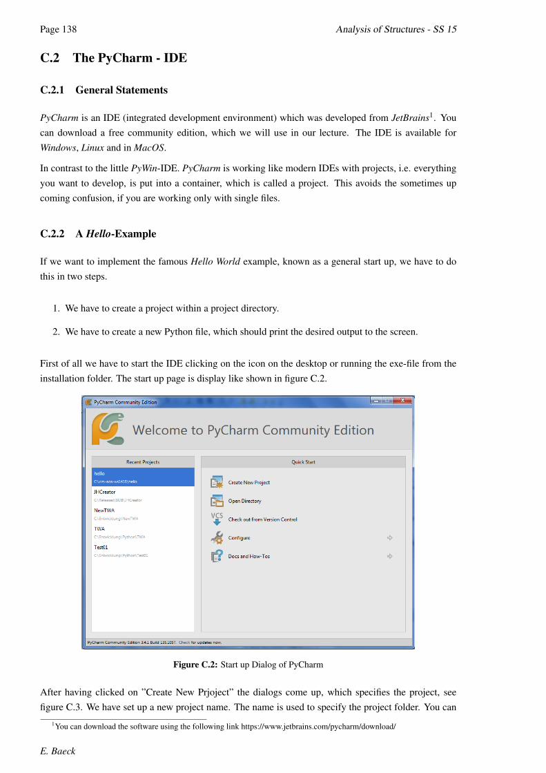
Page 138 Analysis of Structures - SS 15
C.2 The PyCharm - IDE
C.2.1 General Statements
PyCharm is an IDE (integrated development environment) which was developed from JetBrains1. Youcan download a free community edition, which we will use in our lecture. The IDE is available forWindows, Linux and in MacOS.
In contrast to the little PyWin-IDE. PyCharm is working like modern IDEs with projects, i.e. everythingyou want to develop, is put into a container, which is called a project. This avoids the sometimes upcoming confusion, if you are working only with single files.
C.2.2 A Hello-Example
If we want to implement the famous Hello World example, known as a general start up, we have to dothis in two steps.
1. We have to create a project within a project directory.
2. We have to create a new Python file, which should print the desired output to the screen.
First of all we have to start the IDE clicking on the icon on the desktop or running the exe-file from theinstallation folder. The start up page is display like shown in figure C.2.
Figure C.2: Start up Dialog of PyCharm
After having clicked on ”Create New Prjoject” the dialogs come up, which specifies the project, seefigure C.3. We have set up a new project name. The name is used to specify the project folder. You can
1You can download the software using the following link https://www.jetbrains.com/pycharm/download/
E. Baeck
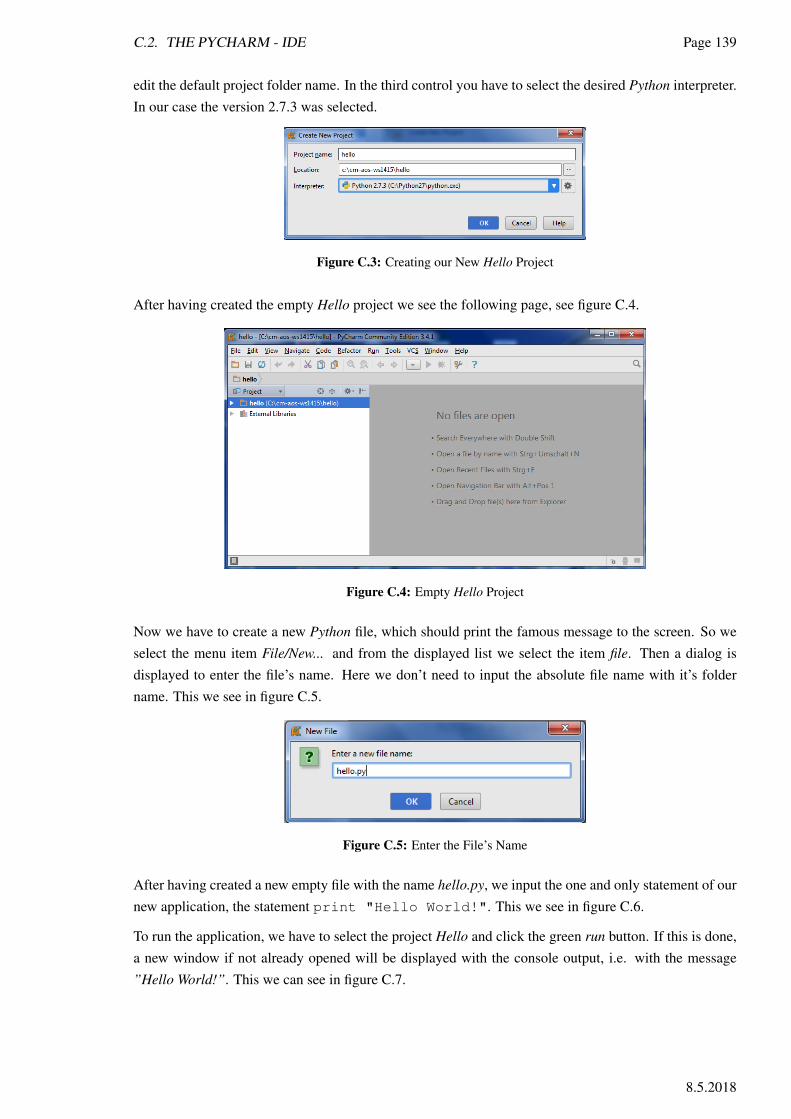
C.2. THE PYCHARM - IDE Page 139
edit the default project folder name. In the third control you have to select the desired Python interpreter.In our case the version 2.7.3 was selected.
Figure C.3: Creating our New Hello Project
After having created the empty Hello project we see the following page, see figure C.4.
Figure C.4: Empty Hello Project
Now we have to create a new Python file, which should print the famous message to the screen. So weselect the menu item File/New... and from the displayed list we select the item file. Then a dialog isdisplayed to enter the file’s name. Here we don’t need to input the absolute file name with it’s foldername. This we see in figure C.5.
Figure C.5: Enter the File’s Name
After having created a new empty file with the name hello.py, we input the one and only statement of ournew application, the statement print "Hello World!". This we see in figure C.6.
To run the application, we have to select the project Hello and click the green run button. If this is done,a new window if not already opened will be displayed with the console output, i.e. with the message”Hello World!”. This we can see in figure C.7.
8.5.2018
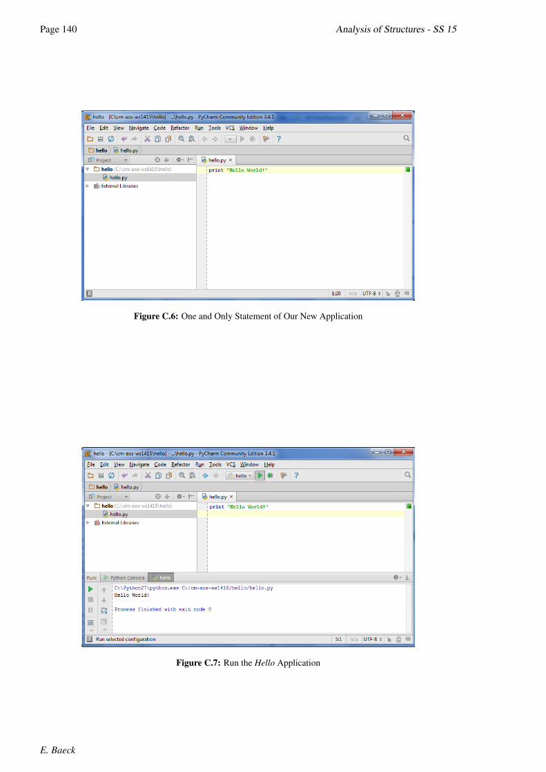
Page 140 Analysis of Structures - SS 15
Figure C.6: One and Only Statement of Our New Application
Figure C.7: Run the Hello Application
E. Baeck

Appendix D
Conventions
D.1 The Java Code Conventions
The following code convention [7] is published by Oracle (successor of Sun Microsystems, Inc). Weapply this convention to choose names for our software items.
1. ClassesClass names should be nouns, in mixed case with the first letter of each internal word capitalized.Try to keep your class names simple and descriptive. Use whole words-avoid acronyms and ab-breviations (unless the abbreviation is much more widely used than the long form, such as URL orHTML).
2. MethodsMethods should be verbs, in mixed case with the first letter lowercase, with the first letter of eachinternal word capitalized.
3. VariablesExcept for variables, all instance, class, and class constants are in mixed case with a lowercase firstletter. Internal words start with capital letters. Variable names should not start with underscore _or dollar sign $ characters, even though both are allowed.
Variable names should be short yet meaningful. The choice of a variable name should bemnemonic- that is, designed to indicate to the casual observer the intent of its use. One-charactervariable names should be avoided except for temporary ”throwaway” variables. Common namesfor temporary variables are i, j, k, m, and n for integers; c, d, and e for characters.
4. ConstantsThe names of variables declared class constants and of ANSI constants should be all uppercasewith words separated by underscores ("_"). (ANSI constants should be avoided, for ease ofdebugging.)
141

Page 142 Analysis of Structures - SS 15
E. Baeck

Appendix E
Parallel Computing
E.1 Threads
The most general parallelisation of code is given in the usage of so called threads. A thread is like anapplication, which is started and which is running then independent of it’s creating program. Threadsare often used, to run some time consuming events in the background of an interactive program. Ifthis activity would not run independent in the background, it would block all interactive events of theapplication, like clicking on buttons or scrolling the window contents and the user would have the feeling,that this application is hanging.
Threads run parallel on one processor using a task switch strategy. For example, if we run a browserand a mailing application on an old computer, we get the feeling, that they are be executed in parallel.With on processor we can not do this. Applications are executed piecewise sequentially. If the hardwarehowever comes with more than one processor, in general the operating system, i.e. Windows in our case,is able to distribute this threads onto all available processor, so that they can be executed in parallel. Thiswe can see, checking the processor loads.
The disadvantage of this kind of threads is, that in general the end of a thread have to be caught bythe caller, so that the caller is able to use the outcome of the thread. This in general costs an effort ofadministration.
E.2 A Multi-Processing Pool
In contrast to general threads we can use a so called Multi-Processing-Pool. This pool is filled thisthreads of the same kind. If the calculation is started, all this threads are executed on a given set ofprocessors. This execution is sequential from the view of the calling program, i.e. the calling program iscalling the Multi-Processing-Pool being executed and will halt until all threads are executed, so that wewill not need a code which is synchronizing the execution of the threads.
A typical use case for this is a simple loop with independent cycles.
A really nice example, which shows the usage of a Multi-Processing-Pool is the calculation of the socalled Mandelbrot set1. This calculation can be split up in several independent cycles. To show the
1Benoı̂t B. Mandelbrot, described the Mandelbrot set as a number of complex numbers.
143

Page 144 Analysis of Structures - SS 15
performance of parallel execution we introduce the TimeCheck class given in the listing .
The Mandelbrot set is given by the following iteration formula.
zn = z2n−1 + c (E.1)
with z, c ∈ C
If the absolute value is less equal two it’s a Mandelbaum set point. Otherwise it’s not. In figure E.1 thePoints of the Mandelbraum set are plotted in the complex number plane.
E.2.1 A Single Processor Solution
The function mandelbrotCalcRow calculates the the data for one row of the Mandelbrot set picture.We put this function partialCalcRow with its function parameters xrange(h) into a map, whichcalculates the values for all function parameters. The function partial is used to reduce the number ofarguments of the function mandelbrotCalcRow simply to one, i.e. the last non set, i.e. the yposargument. So the parameter space is reduced from 4 to 1. For this dimension, i.e. ypos, the map iscreated. On a i7 processor we need 21 seconds to get the result.
Listing E.1: Mandelbrot Single Processor Solution
1 import matplotlib.pyplot as plt # is used to show the results
2 from functools import partial # to create a one dimensional function
3 from TimeCheck import TimeCheck # performance checker
4
5 # calculation of one mandelbrot row
6 def mandelbrotCalcRow(yPos, h, w, max_iteration = 1000):
7 y0 = yPos * (2/float(h)) - 1 # rescale to -1 to 1
8 row = []
9 for xPos in range(w):
10 x0 = xPos * (3.5/float(w)) - 2.5 # rescale to -2.5 to 1
11 iteration, z = 0, 0 + 0j
12 c = complex(x0, y0)
13 while abs(z) < 2 and iteration < max_iteration:
14 z = z**2 + c
15 iteration += 1
16 row.append(iteration)
17 return row
18
19 # creates a set of calculations
20 def mandelbrotCalcSet(h, w, max_iteration = 1000):
21 partialCalcRow = partial(mandelbrotCalcRow, h=h, w=w,
22 max_iteration = max_iteration)
23 mandelImg = map(partialCalcRow, xrange(h))
24 return mandelImg
25
26 # main program calling the mandelbrot calculations
27 # create the timecheck object
28 s = TimeCheck()
29 # and set current time
30 s.set()
31
32 # run the mandelbrot calculation
E. Baeck

E.2. A MULTI-PROCESSING POOL Page 145
33 mandelImg = mandelbrotCalcSet(400, 400, 1000)
34 # print the performance data
35 s.get("single processor performance")
36
37 plt.imshow(mandelImg)
38 plt.savefig(’mandelimg.png’)
39 # plt.show()
Listing E.2: Output for a i7 Processor
1 21.912 : single processor performance
E.2.2 A Multi Processor Solution
If we now want to use the power of our i7 processor, i.e. if we want to use the 4 available cores, we haveto distribute the calculation load of the Mandelbrot set rows onto this cores. This we see in listing E.3.
Listing E.3: Mandelbrot Multi Processor Solution
1 import multiprocessing # is used to get multi processor support
2 import matplotlib.pyplot as plt # is used to show the results
3 from functools import partial # to create a one dimensional function
4 from TimeCheck import TimeCheck # performance checker
5
6 # calculation of one mandelbrot row
7 def mandelbrotCalcRow(yPos, h, w, max_iteration = 1000):
8 y0 = yPos * (2/float(h)) - 1 # rescale to -1 to 1
9 row = []
10 for xPos in range(w):
11 x0 = xPos * (3.5/float(w)) - 2.5 # rescale to -2.5 to 1
12 iteration, z = 0, 0 + 0j
13 c = complex(x0, y0)
14 while abs(z) < 2 and iteration < max_iteration:
15 z = z**2 + c
16 iteration += 1
17 row.append(iteration)
18 return row
19
20 # creates a set of calculations and distributes it onto 4 processors
21 def mandelbrotCalcSet(h, w, max_iteration = 1000):
22 # make a helper function that better supports pool.map by using
23 # only 1 parameter
24 partialCalcRow = partial(mandelbrotCalcRow, h=h, w=w,
25 max_iteration = max_iteration)
26
27 # creates a pool of process, controls worksers
28 pool =multiprocessing.Pool(processes=4)
29
30 # the pool.map only accepts one iterable, so use the partial function
31 # so that we only need to deal with one paramter.
32 # the pool method map runs the set in parallel
33 mandelImg = pool.map(partialCalcRow, xrange(h))
34 pool.close() # we are not adding any more processes and close
35 pool.join() # tell it to wait until all threads are done before going on
36
8.5.2018

Page 146 Analysis of Structures - SS 15
37 return mandelImg
38
39 # check, if thread is main tread!
40 if __name__==’__main__’:
41
42 # main program calling the mandelbrot calculations
43 # create the timecheck object
44 s = TimeCheck()
45 # and set current time
46 s.set()
47
48 mandelImg = mandelbrotCalcSet(400, 400, 1000)
49 # print the performance data
50 s.get("quadcore performance")
51
52 # show result image
53 plt.imshow(mandelImg)
54 plt.savefig(’mandelimg.png’)
Listing E.4: Output for a i7 Processor
1 9.941 : quadcore performance
Figure E.1: Mandelbrot Set
We see that the function mandelbrot-CalcRow in both cases is the same.One difference is, that in multi proces-sor case we use the pool and it’s map.Another difference is, that, if the py-file is executed, the main run must bemarked, that the main program is notmultiple executed.
We see too, that obvious we onlyreach a performance jump of 100%,i.e. the administration of the load dis-tribution needs a lot of power. Thiscomes from the fact, that the pythoninterpreter has to load the file multi-ple, which should be executed in par-allel. If the calculation really splits upinto independent cycles, we would ex-pect nearly a factor of 4 instead of 2.
Figure E.1 shows the result of our calculation. Every cycle is calculating one row of this picture.
E. Baeck

Appendix F
Some Special Abaqus-GUI-Features
In this chapter we talk about some special features of the Abaqus-GUI.
F.1 Viewport Annotations
F.1.1 The Legend’s Font Size
Sometimes the standard parameters of the Abaqus GUI are really unlucky. So the standard font is setto 8 points, i.e. it’s impossible to read the text inside the legend, if we create a standard figure with thefollowing code. The script will plot the calculated displacements colored onto the displaced system. Ina loop we select the displacement related to all coordinate axis.
1 # - create png-files of the displacement components u1, u2, u3 (x,y,z)
2 varlist = ("U1","U2","U3")
3 for var in varlist:
4
5 # - plot the results into the window
6 myViewport.odbDisplay.setPrimaryVariable( \
7 variableLabel=’U’, outputPosition=NODAL,
8 refinement = (COMPONENT,var))
9 myViewport.view.fitView()
10
11 # - and then into an png-file
12 pngfile = prjname + "-" + var
13 session.printOptions.setValues(vpBackground=ON)
14 session.printToFile(fileName=pngfile, format=PNG,
15 canvasObjects=(myViewport,))
If we record the selection of a proper font we can use this code to set the font size automatically. Thefollowing code snippet will do this (see figure F.2).
1 session.viewports[’Viewport: 1’].viewportAnnotationOptions.setValues(
2 triadFont=’-*-verdana-medium-r-normal-*-*-100-*-*-p-*-*-*’,
3 legendFont=’-*-verdana-medium-r-normal-*-*-100-*-*-p-*-*-*’,
4 titleFont=’-*-verdana-medium-r-normal-*-*-100-*-*-p-*-*-*’,
5 stateFont=’-*-verdana-medium-r-normal-*-*-100-*-*-p-*-*-*’)
147
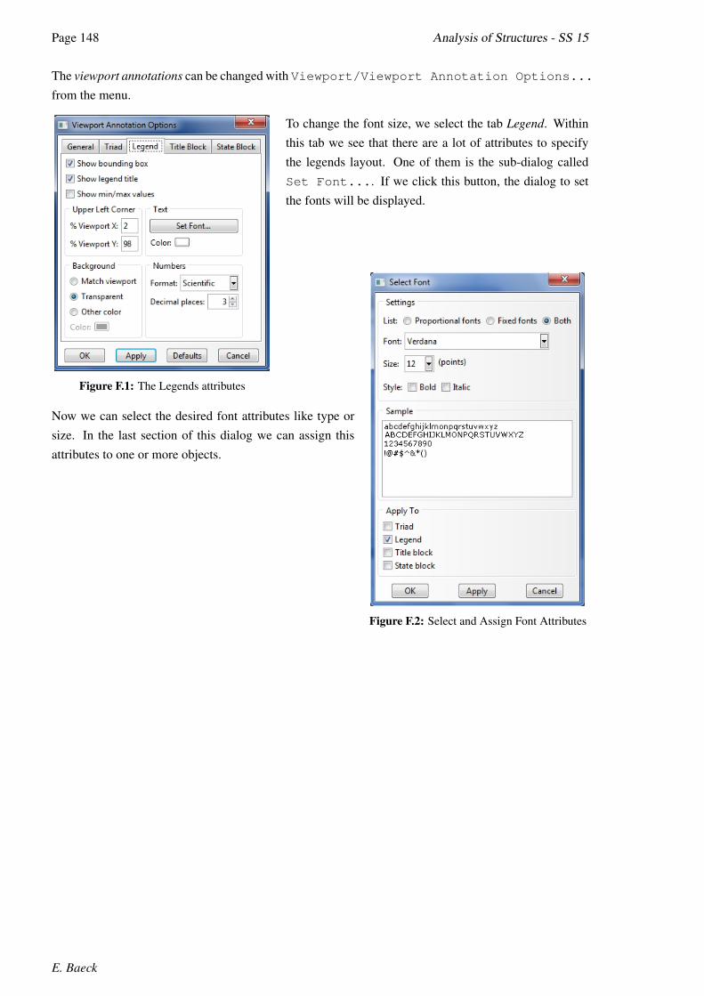
Page 148 Analysis of Structures - SS 15
The viewport annotations can be changed with Viewport/Viewport Annotation Options...
from the menu.
Figure F.1: The Legends attributes
To change the font size, we select the tab Legend. Withinthis tab we see that there are a lot of attributes to specifythe legends layout. One of them is the sub-dialog calledSet Font.... If we click this button, the dialog to setthe fonts will be displayed.
Figure F.2: Select and Assign Font Attributes
Now we can select the desired font attributes like type orsize. In the last section of this dialog we can assign thisattributes to one or more objects.
E. Baeck

F.2. SPECIFY VIEW Page 149
F.2 Specify View
A view can be specified by setting the view direction, called Viewpoint and the Up vector. The Viewpointspecifies the view direction. We should input a vector of this direction. Only the vector direction isimportant not the vector length. The second vector specifies the up direction, so we have to specify thisdirection with a vector again, whose direction only is important.
We can input this data within the following dialog of the View menu (see F.3)..
Figure F.3: Specify the View
In following code we can see, that we select from the session’s viewport container the standard view-port "Viewport: 1". It’s viewmember provides a method to specify the directions discussed above.
1 session.viewports[’Viewport: 1’].view.setViewpoint(viewVector=(1, -1, 1),
2 cameraUpVector=(0, -1, 0))
8.5.2018

Page 150 Analysis of Structures - SS 15
E. Baeck

Bibliography
[1] H.P. Langtangen:A Primer on Scientific Programming with PythonSpringer-Verlag Berlin Heidelberg, 2009
[2] NumPy Community:NumPy User GuideRelease 1.4.1, April 2010
[3] SciPy Community:SciPy Reference GuideRelease 0.8.dev, February 2010
[4] ISO/IEC 19501:2005Information technology – Open Distributed Processing – Unified Modeling Language(UML) Version 1.4.2
[5] D. G. TaggartUniversity of Rhode Island, 2009
[6] O. LuegerLexikon der Technik, 1904
[7] Java Code ConventionsOracle Inc., Sun Microsystems, Inc., September 12, 1997
151

Index
:, 31
AbaqusabaqusMacros, 99BaseWire, 100close, 102ConstrainedSketch, 100DisplacementBC, 101element type
T2D2, 101elemType, 101fieldOutputs, 102frame, 102generateMesh, 101getSequenceFromMask, 100instance, 100job, 101material, 100mesh, 101model, 99openOdb, 102part, 100regionToolset, 101rootAssembly, 100SectionAssignment, 100seedEdgeByNumber, 101session, 101setElementType, 101StaticStep, 101step, 102submit, 101TrussSection, 100values, 102vertices, 101viewport, 101visualization, 102waitForCompletion, 101
append, 41Aptana, 137
area, 133arithmetic mean, 135as, 17
Basic, 24bit’s values, 19break, 28bytecode, 5
C, 5, 19, 23, 24, 27C#, 5Camel Case, 15center of mass, 135Charles Simonyi, 15chdir, 99class
AList, 75, 79Base, 67Element, 71Node, 69Profile, 75ProfileDB, 88, 89UProfile, 75, 84
classes, 55code blocks, 25complement, 18ComTypes, 7conditional assignment, 32constructor, 55continue, 28cos, 17count, 41
datetime, 47day, 48def, 31derivative, 36destructor, 56dictionary, 42, 88
e/E format, 23
152
INDEX Page 153
except, 81exception, 84extend, 41
f format, 23factorial, 27factorial(170), 28factorial(400), 28file
close, 50open, 49read, 50write, 50
Finite Element Model, 95first moment, 133float, 24font size, 147for, 27FORTRAN, 5Fortran, 24
g/G format, 23global variables, 26
hour, 48Hungarian Notation, 15
IDE, 137if, 32import, 17indent, 25index, 41insert, 41int, 24Interactive window, 13iteration, 36
Java, 5Java Code Conventions, 141
legend, 147Lib, 6Lib/site-packages, 88LIFO, 41Linux, 138list, 39, 40, 50Logging, 52long, 24
MacOS, 138main axis, 136Mandelbrot Set, 143Mandelbrot/Multi Processor Solution, 145Mandelbrot/Single Processor Solution, 144map, 42mathplotlib, 46microsecond, 48minute, 48moment of inertia, 134month, 48Monty Python, 5
name, 24negative number, 18Newton, 35Newton’s Algorithm, 38, 62now, 47NumPy, 7
OOP, 53, 107
package, 17, 87Parameters, 31Performance-Checker, 48, 58pi, 17pop, 41printf, 23private, 55, 56push, 41PyDev, 137pylab, 46PythonWin, 12
raise, 84random, 45Random Numbers, 46readlines, 50remove, 41reserved words, 16return, 31reverse, 41
SciPy, 9second, 48second moment, 134Setup, 6
8.5.2018

Page 154 Analysis of Structures - SS 15
sin, 17site-packages, 6sort, 41stack, 41strings, 39Sun Microsystems, Inc., 15
The Beatles, 42timedelta, 47Tkinter, 75try, 81tuple, 31, 39type, 24type checking, 35
UML, 53aggregation, 54class diagram, 53composition, 54inheritance diagram, 54note diagram, 53note diagram assignment, 53
version, 6viewport annotations, 148
while, 27Windows, 138
year, 48
E. Baeck