Analysis of reinforced concrete structures subjected to dynamic loads

Analysis of reinforced concrete structures subjected to dynamicloads with a viscoplastic Drucker±Prager model

Juan Jos�e L�opez Cela 1

Universidad de Castilla-La Mancha, ETS Ingenieros Industriales de Ciudad Real, Campus Universitario s/n, 13071 Ciudad

Real, Spain

Received 23 July 1997; received in revised form 27 April 1998; accepted 2 June 1998

Abstract

The behavior of reinforced concrete structures subjected to dynamic loads is analyzed. The concrete material is

modelled by an elasto-viscoplastic law, whose inviscid counterpart is the Drucker±Prager model. A viscous regular-

ization is introduced in order to avoid the mesh dependency e�ects that usually appear when strain softening occurs.

The model is implemented in a general ®nite element computer code for fast transient analysis of ¯uid-structure sys-

tems, based on an explicit central di�erence scheme. The model is activated to both continuum elements and layered

shell elements. So, realistic numerical analyses of complex 3-D engineering problems are simple and e�cient. Three

examples, two of which are modelled with layered shell elements, are presented below. Ó 1998 Elsevier Science Inc.

All rights reserved.

Keywords: Fast transient analysis; Reinforced concrete; Viscoplastic material law; Layered shell elements

Applied Mathematical Modelling 22 (1998) 495±515

1 Tel.: +34 926 295 300; fax: +34 926 295 361; e-mail: [email protected].

Notation

Mathematical modelr stress tensorr hydrostatic stressc shear stressr0 deviatoric stress tensore strain tensore0 deviatoric strain tensore volumetric strainF �r; a; c� Drucker±Prager yield surfacea; c material parameters de®ning the yield surfaceI identity tensorQ�r;b; c� plastic potential functionb; c material parameters de®ning the plastic potential functionDt time increment

0307-904X/98/$19.00 Ó 1998 Elsevier Science Inc. All rights reserved.

PII: S 0 3 0 7 - 9 0 4 X ( 9 8 ) 1 0 0 5 0 - 1

1. Introduction

The scope of this work is to analyze the behavior of reinforced concrete structures subjected todynamic loads such as impacts, explosions, etc. For the concrete material a Drucker±Pragerelastoplastic model [1] is assumed. This model is relatively simple (only needs two parameters tode®ne the yield surface and one more parameter to de®ne the plastic potential function andconsequently the ¯ow rule) but can reproduce some features considered typical in concrete:softening and di�erent behavior in tension and compression. The softening phenomenon consistsin a reduction of the load-carrying capacity with increasing strain. This results in mesh sensitivityproblems. Regularization procedures are methods for avoiding this sensitivity [2]. One of thesemethods, followed in the present work, is the introduction of viscoplastic terms in the materialconstitutive law [3,4]. The numerical implementation is based on the radial return algorithm [5]generalized for the case of strain hardening or softening [6], as summarized for a von Mises modelin Ref. [7]. A viscoplastic regularization is applied after an inviscid solution has been obtained [8].

M outward normal to the plastic potential functionrf viscoplastic stress tensorq vector of internal variables (a,c for the Drucker±Perger model)g viscoplastic parameterv fastest elastic wave speedl mesh size parameterep equivalent plastic strainep plastic strain tensorLayered shell formulationF int vector of internal nodal forces for a given elementV e volume of an elementB matrix of derivatives of the shape functionsx; y; z coordinatesn; g; f normalized coordinatesW weights of numerical integrationL layer indexNL total number of layersh thickness of the shellhL thickness of layer LuL ratio of the layers thickness to the total thicknessMaterial parametersE Young's modulusv Poisson's ratioq densityryield elastic limitfc maximum compressive strengthft maximum tensile strengthk cohesion/ friction angleW dilatancy angleK bulk modulusG shear modulus

496 J.J. L�opez Cela / Appl. Math. Modelling 22 (1998) 495±515

Since the Drucker±Prager yield surface in stress space is a cone, the developed algorithm includesa speci®c treatment of the stress points that lie close to the cone apex, where the normal to theyield surface is not de®ned.

This material behavior law has been activated to 2-D and 3-D continuum elements but em-phasis has been done in to set up a simple but e�ective method for the numerical representation ofthin reinforced concrete structures. The chosen approach is `macroscopic', in that the structuresto be studied are discretized by shell ®nite elements. A typical element is viewed as a sandwichcomposed of several layers, each one having its own, homogeneous material. For simplicity, noattempt is done to model relative motions of the layers due e.g. to slip or delamination phe-nomena. This of course reduces the applicability of the method to the cases (i.e., load regimes orparts of the time transients) where such extreme phenomena do not play a primary role.

The main advantages of the method are its simplicity and its high computational e�ciency, dueto the fact that a small number of relatively large shell elements are used to model a givenstructure in place of myriads of much smaller continuum elements. Another attractive property isthat it is easily implemented as an extension in any general ®nite element computer code alreadycontaining (homogeneous) shell elements and a library of suitable materials. The formulation issuch that any meaningful combination of layers and materials is easily obtained and the modelcan be used, with the limitations pointed out above, not only for the representation of reinforcedconcrete structures but also more generally for any composite material that admits a layeredapproximation.

A material identi®cation procedure has been developed in order to derive the concrete materialdata de®ning the yield surface from piecewise linearized experimental stress±strain curves. Theprocedure aims at reproducing a uniaxial compression curve and the maximum tension strengthvalue. Two methods have been investigated: in the ®rst one, the hardening or softening regime isobtained by expanding the Drucker±Prager yield surface without changing the angle of the cone.The second method considers only variations of the angle. These evolutions of the yield surfaceare directly related to variations, during the plastic ¯ow, of the two physical parameters of thismodel: cohesion for the ®rst case and friction angle for the second one. In the present study, thesetwo e�ects have been analyzed independently.

The model is implemented in PLEXIS-3C, a general ®nite element code for fast transientanalysis of ¯uid-structure systems [9]. PLEXIS-3C is jointly developed since 1986 by the FrenchCommissariat �a l'Energie Atomique (CEA-CEN Saclay) and by the European Commission (EC-JRC Ispra). The code uses a central di�erence, explicit time marching algorithm which, combinedwith suitable lumping of the mass matrix, leads to a fully explicit implementation. PLEXIS-3Co�ers a large library of ®nite elements, using both continuum and structural representations, andtherefore allows for straightforward implementation of the layer-based technique described in thiswork. In addition, the code presents unique capabilities for the simulation of ¯uid-structure in-teractions. Both the structural and the ¯uid domain can be represented within one single, fullycoupled numerical analysis thanks to sophisticated, yet fully automatic, interfacing algorithms.These are capable of automatically detecting and properly treating even the most complex ¯uid-structure interfaces of the permanent type, see e.g. Ref. [10].

Three numerical examples are presented in this work. The ®rst one, consisting of a reinforcedconcrete slab subjected to an impact load at the center, has been analyzed by using two-dimen-sional continuum elements. The second case is an impact on a natural-draught cooling tower,which is discretized by triangular layered shell elements. The third test case is an example of fullycoupled ¯uid-structure analysis, a gas explosion in a reactor containment. The geometry is axi-symmetric and the structures are modelled with layered conical shell elements, while continuumelements discretize the ¯uids (explosive bubble and air) contained within the reactor building.

J.J. L�opez Cela / Appl. Math. Modelling 22 (1998) 495±515 497

2. Constitutive model for concrete

The constitutive model used in the present study is elasto-viscoplastic. Its inviscid counterpartis the Drucker±Prager model with hardening or softening. A Drucker±Prager model is repre-sented by the two-parameter yield surface

F �r; a; c� � ar� sÿ c � 0; �1�where

r � 1

3tracer hydrostatic stress; �2�

s � 1��2p ��

r0: r0p

shear stress; �3�

r0 � rÿ rI deviatoric stress; �4�where r is the stress tensor, I is the identity tensor and a; c are material parameters related to thefriction angle and the cohesion, respectively.

The numerical implementation of the model is based on the radial return algorithm but bytaking into due account the particularities of a Drucker±Prager model [1]. The main di�erencebetween the two models is the shape of the yield surface in the stress space: while the von Misessurface is a cylinder, the Drucker±Prager surface is a cone. As a consequence, in a Drucker±Prager model an associative plastic ¯ow produces variations in both hydrostatic and deviatoricstress components. The radial return algorithm gives the time-discrete evolution equations for theinviscid solutions rn�1, r0n�1, an�1 and cn�1 at time tn�1 � tn � Dt.

The plastic ¯ow is de®ned according to the plastic potential function:

Q�r;b; c� � br� sÿ c � 0 �5�in the above equation, b is a material parameter related to the dilatancy, representing an inelasticvolume increase. If a � b, an associative ¯ow rule is obtained, otherwise the law is said non-as-sociative.

Another particularity of the Drucker±Prager model is that is necessary to distinguish two zonesin the yield surface:· A normal zone, where the return to the yield surface from the trial stress points is performed

according to the radial return algorithm, but with corrections in the hydrostatic and deviatoricstress components, as indicated above.

· A singular zone, close to the cone apex, where the normal to the plastic potential surface is notde®ned and, therefore, it is not possible to return to it as simply as it is done in the previouszone. This zone is delimited by a cone whose apex coincides with the apex of the Drucker±Pra-ger cone and whose generatrix forms a certain angle (depending on the value of the parameterb) with the cone axis.For the singular zone a special algorithm is developed. The normal to the plastic potential

function, that describes the plastic ¯ow, is

M � oQor� 1

2

r0

s� 1

3bI: �6�

It can be seen that this expression becomes singular at the apex, because s � 0. The return tothe yield surface is decomposed into two parts: the ®rst one is a projection onto the hydrostaticaxis, followed by a translation along this axis until the apex is reached.

In order to obtain the consistency parameter which assures that the ®nal stress state is in theyield surface, we impose the continuity of this parameter along the boundary between the normal


region and the singular one. Since when b � 0, it is not possible to return to the apex from thesingular zone, the model requires a positive value (possibly very small) of b.

The radial return algorithm is based on a backward Euler scheme. This means that to computethe ®nal stress at time n� 1 we need to know, at this time, the normal to the plastic potentialfunction and the consistency parameter. The normal is that corresponding to the trial stress. Tocompute the consistency parameter it is necessary to distinguish if the hardening law is linear ornot. In the most general, non-linear case, the equation of the consistency parameter must besolved by an iteration procedure. When the hardening law is linear, this equation is amenable toclosed form solution. Because in the kind of problems addressed in this work (fast transientdynamics with explicit time integration) the time step is very small, the error produced by alinearization of a non-linear hardening law during the time step is not very important. Then, for alinear hardening law, this implementation and the ones adopted in Refs. [1,3] are the same. Butfor a non-linear hardening law, in the implementation in PLEXIS-3C, it is very important toperform such a linearization in order to maintain the explicit character of the code.

After an inviscid solution has been obtained the viscoplastic correction can be applied. It isimportant to note that this correction is applied a posteriori, and that it is independent of themodel used for the inviscid case and of the kind of algorithm used for solving the equations. Forviscoplasticity, the formulation proposed by Duvaut±Lions [11] extended to accommodatehardening variables [8] is used. By integrating the viscoplastic constitutive model in closed form[8], the following expressions are obtained:

rfn�1 � eÿDt=grn � 1ÿ eÿ

Dtg

h irn�1 �

1ÿ eÿDt=g

Dt=gDr; �7�

qfn�1� eÿ

Dtg q

n� 1ÿ eÿ

Dtg

h iq

n�1; �8�

where q represents a vector of the internal plastic variables, that for the particular case of theDrucker±Prager model includes the two material parameters a and c; Dt is the step increment ofthe central di�erence scheme and g is a viscoplastic parameter having a time dimension.

The viscoplastic model is linear and therefore appears to be very poor in representing possiblestrain rate e�ects. However, it should be recalled that this part of the model acts as a regular-ization of the solution and not as a physical contribution to it. In particular, the g parameter ischosen according to numerical requirements. Being just a regularization, the model should be ascomputationally cheap as possible. It is remarkable that the linear assumption leads to an explicitevaluation of the stresses. In particular, no (conditionally stable) subincrementation algorithmwill have to be included for this evaluation. Because of the application after the inviscid solutionand the integration in closed form, the use of this regularization has a very low computationalcost indeed.

To select the value of the g parameter the criterion proposed in Ref. [4] is followed

lvg6 5; �9�

where v is the fastest elastic wave speed and l is the mesh size parameter, that following commonpractice is taken to be the diameter of the largest element in the mesh.

When g! 0, Dt=g!1 and then rfn�1 ! rn�1 and the inviscid case is recovered. On the other

hand, if g!1Dt=g! 0 and then rfn�1 ! rn � Dr and we have the elastic case. For a given Dt

(®xed with numerical criteria for the central di�erence scheme) it is needed a value of g as low aspossible but su�ciently high to regularize the solution. Then, when a non-zero value of g isadopted, di�erent results than a pure elasto-plastic model will be obtained. It is important to


remark that, when mesh dependency occurs, the results with a elasto-plastic model are numeri-cally possible but are not longer valid. On the other hand an elastic model of the material is not arealistic option. With the current viscoplastic model, the results are not completely accurate, butthe achieved approximation can be considered enough for engineering purposes. In any case, thesimplicity of the model and its computational e�ciency compensates this inconvenient.

3. Modelling of thin shell reinforced concrete structures

The shell ®nite element formulations implemented in PLEXIS-3C have in common the basicassumption that ®bers (straight lines across the thickness of the undeformed element) remainstraight during deformation. This hypothesis is justi®ed by the fact that, in order to be representedby shell elements, the structures must be relatively thin.

Fibers may or may not be initially normal to some element mid-plane, usually called thereference surface. If the orientation of the ®bers with respect to the reference surface is allowed tochange during deformation, then transverse shear strains and stresses are included in the modeland one has a so-called Mindlin±Reissner formulation. Otherwise, no transverse shear e�ects aretaken into account, and one has a Kirchho� formulation.

In the shell formulation, the through-thickness stress is set to zero. In the two examples,concerning shell concrete structures, presented in this work one is modelled with three-nodetriangular plates and the other one with two-node axisymmetric shell elements. For the plateelement, the Mindlin±Reissner formulation is assumed and then, only the component normal tothe plane of the plate is zero. For the conical shell due to the axial symmetry and because this shellfollows Kirchho� theory, the three tangential stresses are zero. Therefore, the only non-zero termsof the stress tensor are the longitudinal and circumferential components, rx and rh.

For any of the shell theories adopted in PLEXIS-3C, the main step in the element formulationis the calculation of the internal nodal forces equivalent to the state of stress over the element,which are then used to solve the equilibrium equations. Use is made of the principle of virtualwork which, at the element level, results in an expression of the type:

F int �ZV e

BTr dV ; �10�

where F int is the vector of internal nodal forces for a given element e; V e is the volume of theelement in the current con®guration, B is the matrix of derivatives of the shape functions and r isthe Cauchy stress tensor.

Because of the special nature of the shell thickness z� � direction, the previous integral is usuallyin the form (x and y being tangent to the reference surface):

F int �Z Z

xy

Zz

BTr dz

0@ 1A dx dy �11�

and, because of the complexity of the functions involved (non-linearity of material behavior, largestrains, etc.) it is often best evaluated numerically:

F int �XNn

n�1

XNg

g�1

WnWg

XNf

f�1

BTrÿ �

ngfWf

" #det J : �12�

The W coe�cients are the weights of the numerical integration process (e.g., Gauss rule) and det Jis the determinant of the Jacobian matrix that describes the transformation of the element volume


into a normalized domain, characterized by the normalized coordinates n, g, f. In this waythe function is evaluated only at a given number of sampling or integration points within theelement.

Let us now compare a homogeneous element with one composed by several layers, see Fig. 1.In the homogeneous case, the stress pro®le across the thickness may assume complex shapesbecause of material non-linearities (e.g., plasticity), but is a continuous function. In the multilayercase, instead, if the materials of the various layers have di�erent properties then the stress pro®lemay become discontinuous across layers. The strain pro®les are continuous in both cases becauseof the assumption of straight ®bers. In order to compute the internal forces, we apply a proceduresimilar to 9, but now to each layer of the element separately

F int �XNn

n�1

XNg

g�1

WnWg

XNL

L�1

uL

XNf

f�1

BTrÿ �

ngfLWfL

" #( )det J : �13�

Here L is the layer index which varies from 1 to NL, the total number of layers. NfL is thenumber of Gauss integration points through the thickness in the layer L and fL the normalizedthickness coordinate for the layer. Finally, uL represents the ratio of the layers thickness hL to thetotal thickness h of the element: uL � hL=h hence

PL uL � 1.

4. Identi®cation of the material parameters

The objective of this section is to determine the material parameters a and c of the Drucker±Prager constitutive law in order to reproduce, as closely as possible, the behavior of concrete. Thepresent identi®cation procedure aims at reproducing the experimental uniaxial curves. In otherwords, when a numerical uniaxial compression/tension test is performed, the resulting stress±strain curves should be as similar as possible to the experimental (real) ones. As a preliminarystep, it is common practice to approximate the continuous experimental curves with piecewiselinear ones.

The Drucker±Prager criterion, characterized by a conical yield surface, can be considered as asmooth approximation to the Mohr±Coulomb criterion, which uses an irregular hexagonal

Fig. 1. Idealization of homogeneous and layered shell structures.


pyramid yield surface. Following Ref. [12], the relations between the material parameters of bothsurfaces are calculated as follows:· The starting point is the Mohr±Coulomb yield surface, where the relation between the material

parameters (cohesion k and friction angle /) and the compressive and tensile strength (fc andft) is given by Mohr's circles:

sin / � fc ÿ ft

fc � ft

; �14�

k � fc 1ÿ sin /� �2cos /

� 1

2

��fcft

p: �15�

· Then, by matching the Drucker±Prager surface to the Mohr±Coulomb surface the desired re-lations are obtained.There are several ways to approximate the two surfaces. If matching is imposed at the apex and

either at point A or at point B on the deviatoric plane (Fig. 2), then in the case of point Amatching, the cone circumscribes the hexagonal pyramid along the compressive meridians, whilein the case of point B matching, the Drucker±Prager surface is circumscribed by the pyramidalong the tensile meridians.

If the two surfaces are made to agree along both compressive and tensile meridians, the re-lations of Table 1 are obtained.

These expressions are valid not only for the elastic limit point of the curve, but for all (plastic)points along the curve. If the expressions of compression ®tting are used, then the maximumcompression value fc is correctly predicted, but the tensile one ft is overestimated (in this par-ticular case, about a 30%, i.e., from 4 to 5.5 MPa). The same conclusions can be applied to theother points. Then, due to the fact that it is not possible to ®t both curves simultaneously, theexamples presented in this work have been performed matching the compression one.

In the case of non-perfect plasticity, the problem arises of writing the material parameters interms of the equivalent plastic strain that is the magnitude used by the model implemented in the

Fig. 2. Fitting between Mohr±Coulomb and Drucker±Prager criteria in the deviatoric plane.


code. To obtain these relations the yield surface is derived with respect to the material parametersand it is substituted in the constitutive rate equations, particularized to the case of uniaxial ex-pressions.

In this work, only one of the two possible material parameters k and / has been consideredvariable while the other one has been kept constant. This corresponds to two di�erent evolutionsof the yield surface, as shown in Fig. 3: expansion of the cone or variation of the angle of thecone. Both cases represent a form of isotropic hardening.

The procedure is the following. The constitutive rate equation can be splitted into deviatoricand volumetric parts:

_r0 � 2G _e0 ÿ G_r0

s_k; �16�

_r � K _eÿ _kKb; �17�where G and K are the shear and bulk moduli, _e and _e0 the volumetric and deviatoric part of therate strain tensor and _k the consistency parameter.

For an uniaxial compression test along, e.g. direction 1 we have:

r � ÿ 1

3r1;

r0 � diag ÿ 2

3r1;

1

3r1;

1

3r1

� �;

s � 1��2p ��

r0: r0p

� r1��3p ;

Fig. 3. Two di�erent evolutions of the yield surface.

Table 1

Fitting between Mohr±Coulomb and Drucker±Prager criteria

Compression ®tting Tension ®tting

a � 2sin /��3p �3ÿ sin /� a � 2sin /��

3p �3� sin /�

c � 3fc�1ÿ sin /��3p �3ÿ sin /� c � 3fc�1ÿ sin /��

3p �3� sin /�


e � ÿe1 � 2e2;

e0 � diag ÿ 2

3e1 � e2� �; 1

3e1 � e2� �; 1

3e1 � e2� �

� �;

where r1 and e1 are the stress and strain along direction 1, and e2 the transversal strain. A tensiontest should be considered if we decide to match the tension curve. Then, Eqs. (16) and (17) be-come:· volumetric rate equation

ÿ 1

3_r1 � K�ÿ _e1 � 2 _e2 ÿ _kb�; �18�

· deviatoric rate equations (there are three deviatoric equations but because they are coincident,we only write one of them)

ÿ 2

3_r1 � ÿ2G

2

3� _e1 � _e2� � 2

��3p

3G _k: �19�

Combining Eqs. (18) and (19)

_r1 � E _e1 �_k3

bÿ��3p� �" #

: �20�

On the other hand, the plastic strain rate tensor is de®ned according to the ¯ow rule as

_ep � _koQ

or� _k

1

2

r0

s� 1

3bI

� ��

_kb

diag bÿ��3p

; b��3p

2;b�

��3p

2

" #�21�

and the equivalent plastic strain is

_ep � 2

3

��_ep: _ep

p�

_k3

��2b2 � 3

q�22�

or

_k � 3_ep��2b2 � 3

q : �23�

Finally, Eq. (20) becomes

_r1 � E _e1 � bÿ ��3p��

2b2 � 3

q _ep

264375: �24�

To obtain the two evolutions above explained independently an expression of the Drucker±Prageryield surface in terms of the cohesion k and friction angle /; is needed. This expression, matchedalong compressive meridians with a Mohr±Coulomb surface, is (Ref. [11])

F � r sin /� s3ÿ sin /

2��3p

� �ÿ k cos / � 0 �25�


and particularizing for an uniaxial compression test, one arrives at

r1 � 2k cos /1ÿ sin /

: �26�

The next step is to derive Eq. (26) with respect to k and /.· Expansion of the yield surface (k variable and / constant)

_r1 � dr1

dkdkdep

_ep � 2 cos /1ÿ sin /

dkdep

_ep �27�

and by eliminating _ep between Eqs. (24) and (27)

dkdep � k0 � E

bÿ ��3p��

2b2 � 3

q 1ÿ sin /2 cos /

_r1

_r1 ÿ E _e1

: �28�

· Evolution of the angle of the cone (k constant and / variable)

_r1 � dr1

d/d/dep

_ep � 2

�1ÿ sin /�d/dep

_ep �29�

and by eliminating _ep between Eqs. (24) and (29)

d/dep � /0 � E

bÿ ��3p��

2b2 � 3

q 1ÿ sin /� �2k

_r1

_r1 ÿ E _e1

: �30�

The necessary steps to perform the ®tting are shown in Table 2 in which the previous equationsare written in discrete form.

With these two ®tting procedures the compression curve is correctly reproduced for every valueof b. However, the tension curve is overestimated and the post-peak regime exhibits a strongdependence on b. For b � 0 (non-associative ¯ow rule) the results are better than with b � a(associative ¯ow rule). In a similar manner, if it is decided to match the tension curve, the samekind of problems will appear in the compression curve. There is no special reason to select one ofthe two curves. Even the code allows the possibility of using both of them: one part of thestructure modelled with parameters obtained from a compression curve and the other with thoseparameters that predict the tension curve. Also, another kind of curve can be suggested: forexample, a triaxial test. In this latter case, none of the two uniaxial curves will be accuratelypredicted. This highlights not only the troubles for this simple model to predict the completebehavior of concrete, but also the big di�culties we ®nd in trying to derive realistic materialparameters.

To obtain the value of b, and because the expression of the potential function (Eq. (5)) issimilar to the expression of the yield one (Eq. (1)), we can use

b � 2 sin W��3p

3ÿ sin W� � ; �31�

where W is the dilatancy angle, which represents an increase of plastic volume under pressure.


5. Numerical examples

Several test cases, using 2-D continuum elements, proposed in Refs. [3,4] have been successfullyreproduced with the present model. The main objective of this calculations was to check thee�ectiveness of the viscoplastic regularization introduced in the material law to obtain mesh in-dependent results. As a further example, a simply supported reinforced concrete slab subjected toan impact load at the centre was considered. The structure is also modelled with 2-D continuumelements in a plane strain situation.

Two additional examples are presented in this section: impact on a cooling tower and gasexplosion in a reactor containment. In these cases, the models of the structures are built withlayered shell elements.

In all computations, the steel is modelled with an elastic-perfectly plastic von Mises materialwhile to represent the concrete the material law is the described above and in some detail in Ref.[13].

The material properties are the following. For the steel, elastic-perfectly plastic behavior withE � 210 GPa, q � 7800 kg/m3, m � 0:3 and ryield � 680 MPa. For the concrete, elastoplastic be-havior with softening, E � 20 GPa, q � 2400 kg/m3, m � 0:2; dilatancy angle W � 10�, maximumcompression strength fc � 40 MPa, maximum tension strength ft � 4 MPa, and softening be-havior de®ned by the compression curve represented in Fig. 4.

Table 2

Material identi®cation procedure

Cone expansion Cone angle variation

Step 1. Compute sin / � �fc ÿ ft�=�fc � ft� Step 1. Compute k � 12

��fcft

pStep 2. For each value of the piecewise linear

compression curve, compute from Eq. (26)

ki � ri�1ÿ sin /�2cos /

Step 2. For each value of the piecewise linear compression curve,

compute from Eq. (26)

/i � �r2i ÿ 4k2�=�r2

i � 4k2�

Step 3. Compute the Drucker±Prager material

parameters a and c

a � 2 sin/��3p �3ÿ sin/�

ci � 3ri�1ÿ sin /��3p �3ÿ sin /�

Step 3. Compute the Drucker±Prager material parameters a and c

ai � 2� sin /�i��3p

3ÿ � sin /�i� �

ci �3ri 1ÿ � sin /�i� ��

3p

3ÿ � sin /�i� �

Step 4. Compute dk=dep� �i � �k0�i for each Dr, Deof the curve:

�ki�0 � Ebÿ ��

3p��

2b2 � 3

q 1ÿ sin /2cos /

DrDrÿ EDe

Step 4. Compute d/=dep� �i � �/0�i for each Dr, De of the curve:

�/i�0 � Ebÿ ��

3p��

2b2 � 3

q 1ÿ sin /2k

DrDrÿ EDe

Step 5. Compute the value of the increment of

equivalent plastic strain for each increment of the k parameter

Step 5. Compute the value of the increment of equivalent plastic

strain for each increment of the / parameter

�Dep�i �Dki

�ki�0�Dep�i �

D/i

�/i�0

Note. Because in the expression of �/i�0 appears sin/ that is variable along the curve some discretization is needed in the linear

branches of the curve.


5.1. Concrete slab subjected to impact load

The problem description is shown in Fig. 4. Only one half of the structure was modelled be-cause of the symmetry and two-dimensional continuum elements with four nodes and four in-tegration points were used to discretize the concrete domain. Plane strain conditions areconsidered.

The reinforcement consisted of 15 steel bars of 18 mm diameter along a 1 m depth of the slab.The equivalent steel area was A � 3817� 10ÿ6 m2 of steel per square meter of concrete. Thediscretization of the steel reinforcement was done with beam/shell elements with the nodes rigidlyattached to the nodes of the continuum elements.

To obtain the model parameters for concrete both yield surface evolutions (variation of theangle of the cone and cone expansion) were used. Because the dilatancy angle W is 10� a non-associative ¯ow rule was considered and b � 0:2.

Three di�erent meshes were used in the study with a value of the viscoplastic parameterg � 1� 10ÿ6. In these conditions, the factor l=vg was 4.12 for the ®rst mesh, 3.09 for the secondone and 2.47 for the last and ®nest one. In all cases it was less than 5, ful®lling Eq. (9).

A ®rst set of computations was performed in order to verify again the e�ectiveness of theviscoplastic correction: unreinforced slab, steel reinforced slab (bottom-only or bottom-and-topreinforcement) and concrete characteristics derived with the two yield surface evolutions ex-plained above. In Fig. 5 the deformed meshes of the unreinforced slab are shown for a compu-tation time of 1.05 ms (corresponding to twenty wave re¯ections across the slab). The results forthe inviscid case are mesh dependent (note that just one row of elements fails in each of themeshes) while those calculated with the viscoplastic regularization avoid this problem. In the restof the analyzed cases, also mesh independent results were obtained.

In Fig. 6 are presented some results in terms of equivalent plastic strain distribution for thesame computation time of 1.05 ms. The presented results are those obtained with bottom rein-forcement only and with the intermediate mesh, i.e. l=vg � 3:09. The concrete characteristics are

Fig. 4. Concrete slab subjected to impact load: problem de®nition.


Fig

.5

.C

on

cret

esl

ab

:d

efo

rmed

mes

hes

for

thre

ed

i�er

ent

elem

ent

size

:(a

)in

vis

cid

case

;(b

)vis

cop

last

icca

se.


calculated according the two possible yield surface evolutions. The following conclusions can bedrawn from this ®gure:· Di�erent strain distributions appear in the two computations.· Lower strain values result in the case of characteristics obtained by varying the angle of the

Drucker±Prager cone. This is due to the fact that when this ®tting is used, the tension curvepresents, in the softening part, higher values than those obtained with the other ®tting, i.e.,the reduction of the load carrying capacity is less pronounced.

· The results obtained considering variations in the angle of the cone seem to be closer to realitythan the ones obtained with the other ®tting, i.e., expansion of the cone.

5.2. Thin shell structures

As an example, consider the frequent case of concrete shell structures having reinforcementgrids placed in two `layers' within the bulk of the concrete material, close to the inner and outersurfaces (this typical layout will be assumed in both numerical examples presented below). If eachgrid has a large number of bars oriented along various directions, it can be approximated by anisotropic steel layer in the model. The layer thickness must be chosen so as to represent the realsteel fraction present in the structure. The shell is then composed of 5 layers, of which 3 are ofconcrete and 2 of steel, see Fig. 7. All layers have 1 integration point along the ®ber, except thecentral one that, because of its thickness, has 2 Gauss points.

Fig. 7. Layered shell element: Location of integration points along the thickness.

Fig. 6. Concrete slab: equivalent plastic strain distributions at 1.05 ms for two possible evolutions of the yield surface.


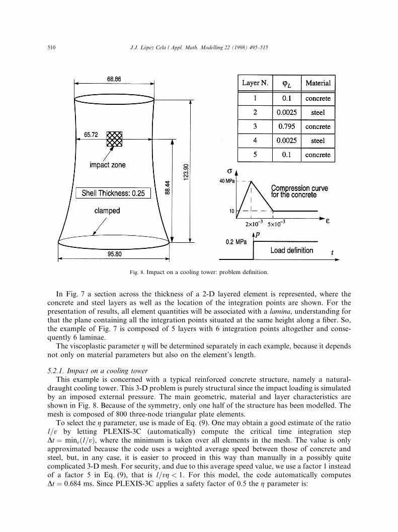
In Fig. 7 a section across the thickness of a 2-D layered element is represented, where theconcrete and steel layers as well as the location of the integration points are shown. For thepresentation of results, all element quantities will be associated with a lamina, understanding forthat the plane containing all the integration points situated at the same height along a ®ber. So,the example of Fig. 7 is composed of 5 layers with 6 integration points altogether and conse-quently 6 laminae.

The viscoplastic parameter g will be determined separately in each example, because it dependsnot only on material parameters but also on the element's length.

5.2.1. Impact on a cooling towerThis example is concerned with a typical reinforced concrete structure, namely a natural-

draught cooling tower. This 3-D problem is purely structural since the impact loading is simulatedby an imposed external pressure. The main geometric, material and layer characteristics areshown in Fig. 8. Because of the symmetry, only one half of the structure has been modelled. Themesh is composed of 800 three-node triangular plate elements.

To select the g parameter, use is made of Eq. (9). One may obtain a good estimate of the ratiol=v by letting PLEXIS-3C (automatically) compute the critical time integration stepDt � mine�l=v�, where the minimum is taken over all elements in the mesh. The value is onlyapproximated because the code uses a weighted average speed between those of concrete andsteel, but, in any case, it is easier to proceed in this way than manually in a possibly quitecomplicated 3-D mesh. For security, and due to this average speed value, we use a factor 1 insteadof a factor 5 in Eq. (9), that is l=vg < 1: For this model, the code automatically computesDt � 0:684 ms. Since PLEXIS-3C applies a safety factor of 0.5 the g parameter is:

Fig. 8. Impact on a cooling tower: problem de®nition.


g >Dt0:5� 1:368� 10ÿ3 ) g � 2� 10ÿ3: �32�

The calculation was performed until a physical time of 100 ms. It required 148 time steps and120 s of CPU on an HP 9000 712 workstation.

In Fig. 9 the equivalent plastic strain distributions are presented for the 4 concrete laminae atthe ®nal time. For ease of comparison, the same scale is used in all drawings. The strongestconcentration of strain is located in lamina 6, that is the internal one. The pressure acts toward thecenter of the tower, so the inner laminae 4 and 6 are under tension in the center and therefore, thehigher values of plastic strain are located in these zones.

5.2.2. Gas explosion in a reactor containmentThis test case is an example of fully coupled ¯uid-structure analysis, a gas explosion within the

reinforced concrete secondary containment building of a nuclear power plant. The geometry ofthe problem is given in Fig. 10 and is assumed to be axisymmetric. The lower basement of thecontainment is very thick and can be modelled by a rigid boundary. The building walls are rel-atively thin and can be conveniently represented by two-nodes conical layered shell elementswithout a topological thickness. The containment is supposed to be initially ®lled by air at roomtemperature and atmospheric pressure. An explosion is assumed to take place in the lower part ofthe building at the initial time of the studied transient.

The explosive is simply represented by a perfect gas at high pressure, which initially occupiesthe zone indicated in black on Fig. 11 (t � 0). The properties of this gas are: density q � 111:5 kg/m3, adiabatic exponent c � 1:4, speci®c internal energy i � 1:28 MJ/kg. The bulk air is also a

Fig. 9. Impact on a cooling tower: equivalent plastic strain distributions for the 4 concrete laminae at 100 ms.


perfect gas with q � 1:2 kg/m3, c � 4 and i � 0:208 MJ/kg. The characteristics of the structuralmaterials are the same as for the previous example, and those corresponding to the layers are inthe table of Fig. 9.

The mesh is composed of 981 continuum ¯uid elements (mostly 4-node quadrilaterals with afew 3-node triangles) and 88 conical shells. In this case, proceeding like in the previous example,one obtains Dt � 0:0213 ms, and therefore the viscosity parameter is

g >Dt0:5� 4:26� 10ÿ3 ) g � 7� 10ÿ5: �33�

The calculation required 11750 steps and 4120 s CPU on an HP 9000 712 workstation, for aphysical time of 250 ms.

Fig. 11 shows the evolution of gas pressure within the containment in the ®rst 120 ms; note thestrong wave propagation and re¯ection e�ects. Fig. 12 shows the deformation of the structure,ampli®ed by a factor 10 to highlight the critical spots. The upper drawings correspond to thepresent case while the lower ones were obtained by assuming a purely elastic homogeneousmaterial for the structure. Note that plasticity is reached in the present models's solution both atthe containment top and, even more pronounced, at the inner horizontal ¯oor, which appears tobe seriously damaged at the end of the computer transient.

Fig. 10. Gas explosion in a reactor containment: problem de®nition.


6. Conclusions

A fully explicit and non-iterative approach to the modelling of reinforced concrete structures,including viscous regularization to avoid mesh sensitivity problems, has been proposed. Theconcrete constitutive law is based on a Drucker±Prager yield criterion with softening or hard-ening. The numerical implementation is based on the classical radial return algorithm. The ex-plicit character of the computer code is maintained even in the case of a non-linear hardening law.This is achieved by performing a linearization in the hardening law during the time step. Due tothe fact that close to the apex of the Drucker±Prager cone exists a singular zone where the returntrajectory is not well de®ned, a special algorithm for the trial stress states that lie in this part of thestress space has been developed. The main assumption is to impose the continuity of the con-sistency parameter along the boundary between the normal region and the singular one. Meshindependent results have been obtained in several test cases modelled with 2-D continuum ele-ments.

For evaluating the concrete material parameters two possible evolutions of the yield surfacewere investigated: more realistic plastic strain distributions were obtained by varying the angle ofthe Drucker±Prager cone rather than by expanding the cone itself. Both yield surface evolutionsrepresent a form of isotropic hardening or softening.

The model has been extended to layered shell elements in order to analyze in a simple bute�cient manner thin reinforced concrete structures. No modelling of the relative motions betweenlayers has been attempted in this formulation. The examples have shown that the method iscorrectly implemented and may be applied to realistic analysis, with plausible results. However, a

Fig. 11. Gas explosion in a reactor containment: ¯uid pressures.


full validation and calibration campaign remains to be done, by comparison with experiments andother data available in the literature.

Acknowledgements

This work has been performed during a post-doctoral Human Capital and Mobility fellowshipat the Institute for Systems, Informatics and Safety of the Joint Research Center of the EuropeanCommission, Ispra, Italy. The author thanks Dr. F. Casadei and Dr. P. Pegon for the helpfuldiscussions while carrying out this work.

References

[1] B. Loret, J.H. Prevost, Accurate numerical solutions for Drucker±Prager elastic-plastic methods, Comp. Meth.

Appl. Mech. Eng. 54 (1986) 259±277.

[2] R. De Borst et al., Fundamental issues in Finite Element analysis of localization of deformation, Eng. Comput. 10

(1993) 99±121.

[3] L.J. Sluys, Wave propagation, localization and dispersion in softening solids, Ph.D. Thesis, Delft University, 1992.

[4] B. Loret, J.H. Prevost, Dynamic strain localization in elasto-(visco)-plastic solids. Part 1. General formulation and

one-dimensional examples. Part 2. Plane strain examples, Comp. Meth. Appl. Mech. Eng. 83 (1990) 247±273 and

275±294.

Fig. 12. Gas explosion in a reactor containment: structural deformations (´10).


[5] M.L. Wilkins, Calculation of elastic-plastic ¯ow, University of California, Lawrence Livermore National

Laboratory, Rep. UCRL-7322 Rev. 1, 1969.

[6] R.D. Krieg, S.W. Key, Implementation of a time-independent plasticity theory into structural computer programs,

in: J.A. Stricklin, K.J. Saczalski (Eds.), Constitutive equations in viscoplasticity: Computational and engineering

aspects (AMD-20), Amer. Soc. Mech. Eng., New York, 1976.

[7] T.J.R. Hughes, Numerical implementation of constitutive models: Rate independent deviatoric plasticity, in:

S. Nemat-Nasser, R.J. Asaro, G.A. Hegemier (Eds.), Theoretical foundation for large-scale computations for

nonlinear material behaviour, Martinus Nujho� Publishers, Boston, MA, 1984, pp. 26±57.

[8] J.C. Simo, J.G. Kennedy, S. Govindjee, Nonsmooth multisurface plasticity and viscoplasticity. Loading/unloading

conditions and numerical algorithms, Int. J. Num. Meth. Eng. 26 (10) (1985) 2161±2185.

[9] H. Bung et al., PLEXIS-3C: A Computer code for fast transient problems in structures and ¯uids, 10th

International Conference in Structural Mechanics in Reactor Technology, SMiRT-10, Anaheim, USA, 14±19

August, 1989.

[10] F. Casadei, J.P. Halleux, An algorithm for permanent ¯uid-structure interaction in explicit transient dynamic,

Comp. Meth. Appl. Mech. Eng. 128 (1995) 231±289.

[11] G. Duvaut, J.L. Lions, Les inequations en Mechanique et Physique, Dunod, Paris, 1972.

[12] W.F. Cheng, Plasticity in reinforced concrete, Mc Graw-Hill, New York, 1982.

[13] J.J. Lopez Cela, P. Pegon, F. Casadei, Fast transient analysis of reinforced concrete structures with Drucker-

Prager model and viscoplastic regularization, in: D.R.J. Owen, E. Onate, E. Hinton (Eds.), Proceedings of the

Fifth International Conference on Computational Plasticity, Fundamentals and Applications, Barcelona, Spain,

17±20 March 1997 (CIMNE).


Analysis of reinforced concrete structures subjected to dynamic loads

Documents

Transcript of Analysis of reinforced concrete structures subjected to dynamic loads