
ANALYSIS OF OPTIONS FOR MARYLAND’S … of Options for Maryland’s Energy Future iii LIST OF...
169
ANALYSIS OF OPTIONS FOR MARYLAND’S ENERGY FUTURE PREPARED BY KAYE SCHOLER LLP LEVITAN & ASSOCIATES, INC. AND SEMCAS CONSULTING ASSOCIATES IN RESPONSE TO TASK #3 REQUEST FOR PROPOSALS PSC #01-01-08 FOR MARYLAND PUBLIC SERVICE COMMISSION NOVEMBER 30, 2007
Transcript of ANALYSIS OF OPTIONS FOR MARYLAND’S … of Options for Maryland’s Energy Future iii LIST OF...

ANALYSIS OF OPTIONS FOR MARYLAND’S ENERGY FUTURE
PREPARED BY KAYE SCHOLER LLP LEVITAN & ASSOCIATES, INC. AND SEMCAS CONSULTING ASSOCIATES
IN RESPONSE TO TASK #3 REQUEST FOR PROPOSALS PSC #01-01-08
FOR MARYLAND PUBLIC SERVICE COMMISSION
NOVEMBER 30, 2007

Analysis of Options for Maryland’s Energy Future i
TABLE OF CONTENTS
I. Executive Summary .............................................................................................................1
A. Overview..................................................................................................................1
B. Definition of Alternative Cases and Key Financial Metrics....................................2
C. Primary Findings......................................................................................................3
D. Environmental Compliance .....................................................................................6
E. Financial Results – Wholesale .................................................................................7
F. Financial Results – Retail ......................................................................................12
G. Conclusions............................................................................................................14
II. Overview............................................................................................................................15
A. Background and Purpose .......................................................................................15
B. Modeling Framework.............................................................................................17
C. External Conditions and Variables ........................................................................22
1. Fuel Price Outlook .....................................................................................22 2. Natural Gas Infrastructure..........................................................................40 3. PJM Jurisdictional Issues...........................................................................43 4. Environmental Compliance .......................................................................56
D. Electricity Market Model Structure .......................................................................63
1. MarketSym Model of Energy Markets ......................................................64 2. Capacity Price Model.................................................................................67 3. Ancillary Services......................................................................................74 4. Wholesale and Retail Financial Model ......................................................74 5. Other Modeling Assumptions ....................................................................75
III. Supply and Demand-Side Options.....................................................................................76
A. Overview of Maryland Options .............................................................................76
B. Contractual and Ownership Options......................................................................77
1. Merchant Facilities.....................................................................................77 2. Third Party Contract Structures .................................................................78 3. Utility-Owned Generation .........................................................................80 4. State Authority Ownership or Contracting ................................................81
C. Technology Options...............................................................................................81
1. Peaking Technologies ................................................................................82 2. Intermediate Load Technologies................................................................83 3. Base Load Technologies ............................................................................84 4. Renewable Energy Resources....................................................................86
D. Demand-Side Management....................................................................................94

Analysis of Options for Maryland’s Energy Future ii
1. Introduction................................................................................................94 2. EMPower Maryland: The “15 by 15” Initiative ........................................97 3. DSM Programs Proposed By Utilities .....................................................100 4. Calculation of Energy and Peak Demand Savings ..................................102 5. Calculation of Program and Participant Costs .........................................104
IV. Economic Analysis of Selected Options..........................................................................105
A. Overview of Analytical Approach .......................................................................105
B. Reference Case Definition ...................................................................................106
1. Modeling Results .....................................................................................108
C. Alternative Case Definitions................................................................................112
1. Optimum Mix Case..................................................................................112 2. Coal Case .................................................................................................114 3. Nuclear Case ............................................................................................118 4. 15 by 15 DSM Case .................................................................................122 5. Transmission Case ...................................................................................127 6. Wind Case................................................................................................132 7. 1200 MW Combined Cycle – “Overbuild” Case.....................................136
D. Comparison of Case Results ................................................................................139
1. Wholesale Energy Prices .........................................................................139 2. Market Capacity Prices ............................................................................142 3. Generation Service Cost Results..............................................................145 4. Benefit and Cost Allocations by Utility and Rate Class ..........................150
V. Conclusions......................................................................................................................157

Analysis of Options for Maryland’s Energy Future iii
LIST OF FIGURES
Figure E-1. Reference Case Annual Costs......................................................................... 8 Figure E-2. Present Value Cost Comparison by Case ....................................................... 8 Figure E-3. Cumulative Present Value .............................................................................. 9 Figure E-4. EVA by Component – Generation Cases ..................................................... 10 Figure E-5. EVA by Component – Non-Traditional Cases ............................................. 11 Figure E-6. Change in Allocated Power Supply Cost – Allegheny................................. 12 Figure E-7. Change in Allocated Power Supply Cost – BGE.......................................... 13 Figure E-8. Change in Allocated Power Supply Costs – Delmarva ................................ 13 Figure E-9. Change in Allocated Power Supply Costs – PEPCO.................................... 14 Figure 10. Study Framework ........................................................................................... 18 Figure 11. Fuel Price Forecast – Annual Average Prices (Nominal $/MMBtu) ............. 25 Figure 12. Base Case WTI Forecast (Nominal $/Barrel)................................................. 27 Figure 13. Fuel Oil Price Forecasts (Nominal $/MMBtu)............................................... 28 Figure 14. Long-Term Forecast of U.S. Gas Production and Consumption.................... 30 Figure 15. Long Term Forecast of Natural Gas Prices at the Henry Hub and PJM ........ 32 Figure 16. Forecast of Coal Prices by Supply Basin ....................................................... 33 Figure 17. Nuclear Fuel Price Forecast............................................................................ 35 Figure 18. Peak Oil Case – WTI Forecast ....................................................................... 37 Figure 19. Natural Gas Forecast – Peak Oil Case............................................................ 38 Figure 20. Low Oil Case – WTI Forecast........................................................................ 39 Figure 21. Natural Gas Forecast – Low Oil Case ............................................................ 40 Figure 22. Nameplate Generating Capacity in Maryland by Fuel Type.......................... 41 Figure 23. Interstate Natural Gas Infrastructure in Maryland.......................................... 42 Figure 24. Monthly LNG Receipts at the Cove Point Import Terminal .......................... 43 Figure 25. Maryland Utilities........................................................................................... 44 Figure 26. Average Annual LMPs in Maryland .............................................................. 45 Figure 27. Sample Variable Resource Requirement Curve ............................................. 46 Figure 28. Locational Delivery Areas for Transition Delivery Years ............................. 47 Figure 29. Amos-Kemptown and 502 Junction-Loudoun Transmission Lines............... 53 Figure 30. Susquehanna-Roseland Transmission Line.................................................... 54 Figure 31. PEPCO Holding Inc. Delmarva (MAPP) Transmission Line ........................ 55 Figure 32. Solar RPS Requirement.................................................................................. 57 Figure 33. Maryland Tier 1 REC Price Forecast ............................................................. 59 Figure 34. CO2 Allowance Price Forecast ....................................................................... 62 Figure 35. NOx and SO2 Price Allowance Forecasts ....................................................... 63 Figure 36. Market Topology............................................................................................ 65 Figure 37. Historical Energy Price Spreads for Delmarva and Other EMAAC Zones ... 66 Figure 38. Historical Energy Price Spreads for the Four Utility Zones in Maryland...... 67 Figure 39. Indicative Supply and Demand Curves .......................................................... 69 Figure 40. Shifts in Supply and Demand Curves............................................................. 70 Figure 41. PJM Load Report Forecast ............................................................................. 71 Figure 42. Reference Case Capacity Additions ............................................................... 72 Figure 43. Long-Term UCAP Prices – Reference Case .................................................. 73 Figure 44. Postulated Solar PV Installations in Maryland............................................... 88

Analysis of Options for Maryland’s Energy Future iv
Figure 45. Solar Module Retail Price Index – U.S. and Europe...................................... 89 Figure 46. New Competitive Equilibrium Following Implementation of DSM.............. 96 Figure 47. Composite Energy Savings Profile............................................................... 104 Figure 48. Reference Case Capacity Additions ............................................................. 107 Figure 49. Reference Case Energy Prices...................................................................... 109 Figure 50. Reference Case Load at Market Energy Price.............................................. 110 Figure 51. UCAP Price Forecast – Reference Case....................................................... 111 Figure 52. Reference Case Annual Costs ...................................................................... 112 Figure 53. Annual Cost Savings – Optimum Mix Case................................................. 114 Figure 54. Ratepayer-Backed Capacity – Coal Case ...................................................... 115 Figure 55. Wholesale Energy Prices -- Coal Case.......................................................... 116 Figure 56. Differential Capacity Prices – Coal Case ...................................................... 117 Figure 57. Annual Cost Savings – Coal Case ................................................................. 118 Figure 58. Ratepayer-Backed Capacity – Nuclear Case................................................. 119 Figure 59. Nuclear Case Energy Prices .......................................................................... 120 Figure 60. Differential Capacity Prices – Nuclear Case ................................................. 121 Figure 61. Annual Cost Savings – Nuclear Case............................................................ 122 Figure 62. 15 by 15 DSM Case Capacity Changes........................................................ 124 Figure 63. 15 by 15 DSM Case Energy Prices .............................................................. 125 Figure 64. Differential Capacity Prices – 15 by 15 DSM Case ..................................... 126 Figure 65. Annual Cost Savings – 15 by 15 DSM Case................................................ 127 Figure 66. Transmission Case Capacity Changes.......................................................... 129 Figure 67. Transmission Case Energy Prices ................................................................ 130 Figure 68. Differential Capacity Prices – Transmission Case ....................................... 131 Figure 69. Annual Cost Savings – Transmission Case .................................................. 132 Figure 70. Ratepayer-Backed Capacity – Wind Case..................................................... 133 Figure 71. Differential Capacity Prices – Wind Case..................................................... 134 Figure 72. Annual Cost Savings – Wind Case............................................................... 135 Figure 73. Breakout of Off-Shore, On-Shore Effects .................................................... 135 Figure 74. Ratepayer-Backed Capacity – Overbuild Case ............................................ 136 Figure 75. Wholesale Energy Prices – Overbuild Case................................................. 137 Figure 76. Capacity Prices – Overbuild Case ................................................................ 138 Figure 77. Annual Cost Savings – Overbuild Case ....................................................... 139 Figure 78. APS Zone Average Energy Prices – All Cases ............................................. 140 Figure 79. EMAAC Zone Energy Prices – All Cases..................................................... 141 Figure 80. SWMAAC Zone Energy Prices – All Cases ................................................. 141 Figure 81. MTM Price Effects on Total Utility Load in Maryland – Alternative Cases142 Figure 82. Capacity Prices – APS, All Cases ................................................................ 143 Figure 83. Capacity Prices – Delmarva, All Cases........................................................ 144 Figure 84. Capacity Prices – BGE/PEPCO, All Cases .................................................. 145 Figure 85. Total Cost Comparison................................................................................. 146 Figure 86. Annual Savings for Alternative Cases.......................................................... 147 Figure 87. Cumulative PV of Annual Savings (EVA)................................................... 148 Figure 88. Cumulative EVA – Alternative Cases Only.................................................. 148 Figure 89. EVA by Component – Generation Cases ...................................................... 149 Figure 90. EVA by Component – Non-Traditional Cases.............................................. 150

Analysis of Options for Maryland’s Energy Future v
Figure 91. Change in Allocated Power Supply Cost – APS........................................... 155 Figure 92. Change in Allocated Power Supply Cost – BGE ......................................... 155 Figure 93. Change in Allocated Power Supply Costs – Delmarva ................................ 156 Figure 94. Change in Allocated Power Supply Costs – PEPCO ................................... 157

Analysis of Options for Maryland’s Energy Future vi
LIST OF TABLES
Table 1. Initial Gross CONE Values ($/MW-day) .......................................................... 48 Table 2. RPM Global and Zonal LDAs ........................................................................... 49 Table 3. Initial RPM BRA Schedule................................................................................ 50 Table 4. RPM Base Residual Auction Results ($/MW-Day) .......................................... 50 Table 5. 2009/10 RPM Results ........................................................................................ 68 Table 6. Merchant Plant Financing Structure and Costs.................................................. 77 Table 7. Merchant, Utility-Owned, and Utility-Supported Plant Financing Costs.......... 79 Table 8. Cost and Operating Parameters for Technology Alternatives (2007 $)............. 82 Table 9. Characteristics of Renewable Generation (2007$) ............................................ 87 Table 10. DOE Wind Classifications................................................................................ 93 Table 11. UCAP Values and Capacity Factors for Wind Projects in Maryland.............. 94 Table 12. EmPower Maryland Statewide Electric Usage Reduction Goal...................... 97 Table 13. Upward-Sloping DSM Supply Curve Assumptions ...................................... 103 Table 14. Reference Case DSM Assumptions............................................................... 108 Table 15. 15 by 15 DSM Case Incremental Effects....................................................... 123 Table 16. Typical Residential Annual Bill – APS ......................................................... 151 Table 17. Typical Residential Annual Bill – BGE ........................................................ 152 Table 18. Typical Residential Annual Bill – Delmarva................................................. 153 Table 19. Typical Residential Annual Bill – PEPCO.................................................... 154

Analysis of Options for Maryland’s Energy Future vii
GLOSSARY
a-Si Amorphous Silicon
AC Alternating Current
ACP Alternative Compliance Payment
APS Allegheny Power System
ARR Auction Revenue Rights
Bbl Barrel
BGE Baltimore Gas & Electric
BRA Base Residual Auction
BWR Boiling Water Reactor
C&I Commercial and Industrial
c-Si Crystalline Silicon
CAIR Clean Air Interstate Rule
CAPP Central Appalachian Basin
CC Combined Cycle
CELP Community Energy Loan Program
CETL Capacity Emergency Transfer Limit
CETO Capacity Emergency Transfer Objective
CFB Circulating Fluidized Bed
CfD Contract for Differences
CFL Compact Florescent Light
CO2 Carbon Dioxide
CONE Cost of New Entry
CPI-U Consumer Price Index – Urban Consumers
CPV Concentrating Photovoltaic
CTR Capacity Transmission Right
DAM Day-Ahead Market
DC Direct Current
DHCD Department of Housing and Community Development
DHR Department of Human Resources
DOE Department of Energy
DPL Delmarva Power and Light
DR Demand Resource
DSM Demand Side Management
DTI-SP Dominion South Point
E&P Exploration and Production
E3 Energy and Environmental Economics, Inc.
Eastern Eastern Shore Natural Gas Shore Company
EE Energy Efficiency
EIA Energy Information Agency
EMAAC Eastern Mid-Atlantic Area Council
EMD EmPower Maryland
EPA Environmental Protection Agency
EPAct Energy Policy Act
EPC Engineering Procurement and Construction
EPR Evolutionary Power Reactor
ESP Electrostatic Precipitators
ESPC Energy Savings Performance Contracting
EVA Economic Value Added
FERC Federal Energy Regulatory Commission
FGD Flue Gas Desulfurization
FMV Fair Market Value

Analysis of Options for Maryland’s Energy Future viii
FSU Former Soviet Union
FTR Financial Transmission Rights
GE General Electric
GPCM Gas Pipeline Competition Model
GPCMdat GPCM Proprietary Database
GSC Generation Service Cost
GT Gas Turbine
GWh Gigawatt Hour
HAA Healthy Air Act
HRSG Heat Recovery Steam Generator
HVAC Heating, Vacuuming and Air Conditioning
ICAP Installed Capacity
IEA International Energy Agency
IEO International Energy Outlook
IGCC Integrated Gasification Combined Cycle
IOU Investor Owned Utility
IPA Illinois Power Agency
IRM Installed Reserve Margin
ISO-NE Independent System Operator – New England
kV Kilovolt
kW Kilowatt
kWh Kilowatt Hour
LAI Levitan & Associates, Inc.
LDA Locational Delivery Area
LIPA Long Island Power Authority
LMP Locational Market Price
LNG Liquefied Natural Gas
LSE Load-Serving Entity
m Meter
MAAC Mid-Atlantic Area Council
MACRS Modified Accelerated Cost Recovery System
MAPP Mid-Atlantic Power Pathway
MEA Maryland Energy Administration
MM Million
MMBtu Million British thermal units
MMS Mineral Management Service
MTM Mark-to-Market
MW Megawatt
MWh Megawatt hour
NAAQS National Ambient Air Quality Standards
NAPP Northern Appalachian Basin
NERC North American Reliability Corporation
NIETC National Interest Electric Transmission Corridor
NOAA National Oceanic and Atmospheric Administration
NOx Nitrogen oxides
NRC Nuclear Regulatory Commission
NYISO New York Independent System Operator
NYMEX New York Mercantile Exchange
NYSERDA New York State Energy Research and Development Authority
O&M Operating and Maintenance
OPEC Organization of the Petroleum Exporting Countries

Analysis of Options for Maryland’s Energy Future ix
PACE PACE Global Energy Services
PEPCO Potomac Electric Power Company
PJM PJM Interconnection
PPA Power Purchasing Agreement
PRB Powder River Basin
PSC Public Service Commission
PTC Production Tax Credit
PV Potovoltaic
PWR Pressurized Water Reactor
REC Renewable Energy Credit
RGGI Regional Greenhouse Gas Initiative
RIWINDS Rhode Island Wind Study
RMR Reliability Must Run
RPM Reliability Pricing Model
RPS Renewable Portfolio Standard
RTEP Regional Transmission Expansion Plan
RTM Real Time Market
RTO Regional Transmission Organization
SCR Selective Catalytic Reduction
SO2 Sulfur Dioxide
SOM State of the Market
SWMAAC Southwest Mid-Atlantic Area Council
Tetco M3 Texas Eastern Transmission Mid-Point
TIPS Treasury Protected Securities
TO Transmission Owner
Transco Transcontinental Gas Pipeline
TZ6-NNY Transco Zone 6 Non-New York
U3O8 Uranium
UCAP Unforced Capacity
U.S. United States
VRR Variable Resource Requirement
WCSB Western Canada Sedimentary Basin
WTI West Texas Intermediate
Analysis of Options for Maryland’s Energy Future 1
TASK 3:
ANALYSIS OF OPTIONS FOR MARYLAND’S ENERGY FUTURE
I. Executive Summary
A. Overview
In this analysis we quantify the costs and benefits of both conventional and unconventional resource options that are available to meet the State of Maryland’s long-term energy requirements. Each option has distinct advantages and disadvantages that policymakers should evaluate before embracing one energy future over another. Some resource options can be combined to help secure Maryland’s long-term energy requirements. Others could operate at cross-purposes and may be mutually exclusive. Across the broad field of resource options available to promote grid security and economic objectives, the primary objective of this study is to provide data and market intelligence that can assist State policymakers in making choices among resource options available to meet Maryland’s long term electricity requirements. Hence, we have calculated the expected economic benefits associated with an array of generation, transmission, and demand-side options to serve Maryland’s energy future.
In order to identify economic benefits for each resource option, we have compared how each generation, transmission, or demand-side option compares on a present value basis to the total cost of serving Maryland’s electricity load under business-as-usual conditions. Throughout this report, these business-as-usual conditions are the Reference Case. For the Reference Case, we assume that the only generation added to the supply mix over the next twenty years will be low-cost, low-risk, simple cycle gas turbines (“peakers”). We have also assumed that the peaker additions do not require long term contracts, in other words, they will be constructed by merchant developers solely in response to wholesale market price signals. And, finally, we have assumed that the amount of additional peaking generation added in the Reference Case will be just enough to meet and maintain the minimum grid reliability requirement in Maryland. In reviewing our results, it is important to note that merchant generators have added very little new generation in Maryland since 2000, when the State’s utilities either divested or transferred their generation assets to unregulated affiliates. While the definition of the Reference Case itself includes a number of uncertain assumptions about Maryland’s long-term energy future, it is nevertheless a reasonable yardstick to measure the costs and benefits that can be ascribed to each evaluated resource option.
The Reference Case represents Maryland’s existing generation resource mix, transmission infrastructure, and a limited level of demand side management (“DSM”), but no new initiatives to foster an increase in generation supply or a decrease in electricity demand. For the Reference Case, we have incorporated about one-fourth of the total DSM objective associated with Governor O’Malley’s “15 by 15” Initiative – a

Analysis of Options for Maryland’s Energy Future 2
15% reduction in per capita energy demand by 2015 – which the State may be able to achieve with existing programs. Because the Reference Case limits resource additions to peakers through 2027, it does not include new high-voltage transmission “highway” projects, new combined-cycle or coal plants, new in-State renewable energy resources (e.g., wind), or a new nuclear plant. In terms of renewable energy, we assumed in the Reference Case that each Maryland utility will continue to comply with Maryland’s renewable portfolio standard (“RPS”), but will meet only the mandatory solar component through photovoltaic additions within Maryland.
B. Definition of Alternative Cases and Key Financial Metrics
Based on consultations with the Maryland Public Service Commission (the “PSC”), we defined seven alternative resource futures to address Maryland’s long-term energy requirements. Each resource option is technologically feasible and, if implemented, can diversify Maryland’s energy infrastructure, thereby providing reliability and economic benefits. Again, although some alternative resource futures may be mutually exclusive, others can be integrated into a diversified resource strategy that achieves a reasonable balance between reliability and economic objectives to keep pace with Maryland’s long-term electricity requirements. The seven Alternative Cases are:
Optimum Mix – We substituted more efficient but more expensive combined cycle generation plants for one or more peakers over the planning horizon whenever market conditions warrant. We assume that the addition of a combined cycle plant would require a long-term contract with Maryland’s utilities.
Coal – We added a 648 MW supercritical pulverized coal plant with state-of-the-art pollution controls in lieu of an equivalent amount of peakers. We assume that the new coal plant would achieve commercial operation in 2015 under long-term utility agreements authorized by the PSC.
Nuclear – We added a new 1,600 MW reactor unit at Constellation’s Calvert Cliffs facility. We assume that the new nuclear plant would achieve commercial operation in 2017 under long-term agreements with Maryland’s utilities.
15 x 15 DSM – We added ambitious conservation and load management initiatives in the form of utility-sponsored programs and regulatory mandates. These programs reduce Maryland’s dependence on new peakers to ensure adequate supply but are primarily oriented to achieving more efficient use of energy around-the-clock. We assume that the utilities’ earnings are decoupled from DSM programs so that they have an incentive to promote load reduction. We have quantified total program costs, including residential and commercial costs that are independent of utility programs in order to achieve the full “15 by 15” Initiative.

Analysis of Options for Maryland’s Energy Future 3
Transmission – We added one new backbone or “highway” transmission project that will begin serving Maryland in 2015, thereby alleviating congestion and promoting grid reliability throughout the region. The addition of a major new transmission project would lessen Maryland’s dependence on new peakers from 2015 throughout the remainder of the study horizon. Under transmission ratemaking principles approved by the Federal Energy Regulatory Commission, the cost of new transmission would be apportioned among ratepayers in Maryland and ratepayers elsewhere in PJM.
Wind – We added 500 MW of new wind turbines, both onshore and offshore by 2012. Because wind is an intermittent generation resource, only about one-fifth of the total nominal installed capacity can be treated as dependable capacity. Therefore the wind turbines only slightly reduce the need for new peakers to maintain grid reliability. Like the other resource options that comprise the Alternative Cases, we assume that the addition of new wind generation would require long-term agreements authorized by the PSC between wind developers and Maryland’s utilities.
Overbuild – We added a generation reserve surplus of 1,200 MW beginning in 2011. We assume that the reserve surplus will consist of new combined cycle plants in Maryland and will be sustained through the study horizon. Both the 1,200 MW of combined cycle plants as well as gas turbine peakers added later to the resource mix would require long-term contracts with the utilities. (Throughout this report, we refer to the Overbuild case and the 1,200 MW case synonymously.)
The difference in the cost to serve Maryland’s load between the Reference Case and each Alternative Case represents the aggregated net benefit or cost of the postulated resource option. We calculated the present value of this net benefit or cost over the study period, 2008 through 2027, using as our primary financial metric the Economic Value Added (“EVA”). EVA is the present value of the net benefit or cost relative to the total cost to serve load in the Reference Case. EVA therefore represents the change or difference in cost to serve load in Maryland under the wholesale market prices simulated for each resource option versus the Reference Case.
C. Primary Findings
Our primary findings are as follows:
In terms of electricity prices, Maryland is and will remain vulnerable to variations in world oil and North American natural gas prices for the foreseeable future. Although Maryland’s existing generation resource base is reasonably well diversified under current economic and environmental conditions, the existing market rules and transmission limitations governing how wholesale energy prices are set in Maryland mean that premium fossil

Analysis of Options for Maryland’s Energy Future 4
fuel costs will continue to dictate both wholesale and retail electricity prices during on-peak hours.
Energy prices in Maryland will likely continue to be influenced greatly by the delivered cost of natural gas and, to a lesser extent, the cost of residual fuel oil to power plants in the region. Historically, natural gas costs have been correlated with oil prices. This statistical relationship has recently broken down as global oil prices have skyrocketed, while natural gas prices have remained high but comparatively stable in response to market dynamics across North America. The long term outlook for world oil prices reflects a continuation of high prices, high volatility, and extreme uncertainty. This view reflects the emergence of China and India as major importers, continued global tensions affecting supplies from the Middle East and, to a lesser extent, Venezuela, and the present lack of technology substitutes for transportation fuels around the world. The long-term outlook for natural gas prices across the Atlantic seaboard reflects a growing gap in the U.S. between robust demand and indigenous continental supplies. While the anticipated supply deficit can be “plugged” through increased reliance on imported liquefied natural gas (“LNG”), the U.S. will need to compete with Europe and Asia for LNG supplies that originate in the Middle East, the Former Soviet Union, Africa, and Trinidad. Over the long-term we expect natural gas prices to remain high by historic standards and also extremely volatile.
Our analysis identified several promising resource options that can satisfy Maryland’s long-term energy requirements. The economic results for new nuclear, a new transmission highway, and DSM are very positive. A sustained capacity overbuild with excess gas-fired generation through 2027 produces less positive, but still potentially attractive economic results but would not reduce the State’s reliance on natural gas. A large, state-of-the-art coal plant also offers a promising resource option from the standpoint of economics and reliability, but those results must be weighed against coal generation’s adverse impact on the goal of reducing greenhouse gas emissions. Optimizing the type of new gas-fired generation or the addition of wind generation produce marginally positive or even negative economic outcomes.
The following specific options warrant additional consideration:
A new nuclear unit at Calvert Cliffs would provide both a physical and financial hedge against the fundamental uncertainty associated with premium fossil fuel prices over the long term. The EVA for the Nuclear Case is $2.9 billion. Of critical importance, the EVA for the Nuclear Case is very sensitive to variations in fuel prices. To the extent oil and natural gas prices are higher than those used in the Base Case fuel price forecast incorporated in the Reference Case, project EVA would be higher than $2.9 billion. The opposite is also true, namely, if oil and natural gas prices are lower than those used in the

Analysis of Options for Maryland’s Energy Future 5
Base Case forecast, project EVA would be lower. Assuming our Base Case fuel price forecast, the benefit-to-cost ratio is 2.1. In light of the chronic uncertainty concerning fossil fuel prices over the long-term, rigorous analysis is needed in order to gauge the “quality” or robustness of the economic benefits as well as the value of the financial hedge from Maryland’s ratepayers’ perspective. From the standpoint of capital at-risk, it would be better for Maryland’s ratepayers if Constellation were to proceed on a merchant basis utilizing federal loan guarantees to attract debt capital. In that case, the capital at-risk would be borne on Constellation’s balance sheet or transferred to third party investors rather than be shifted to Maryland’s ratepayers under iron-clad power purchase agreements. Of course, if Constellation were to merchandise the generation output from a new nuclear plant at Calvert Cliffs, the energy profits would also accrue predominantly to Constellation rather than Maryland’s ratepayers.
The PJM-approved 502 Junction to Loudoun transmission project
would produce substantial economic and reliability benefits in Maryland. The EVA for the Transmission Case is $2.2 billion, and the benefit-to-cost ratio of 21.4. The benefit-to-cost ratio is so high because the cost of transmission would be socialized across all of PJM rather than be apportioned wholly to Maryland. Despite streamlined transmission permitting procedures that Congress enacted under the Energy Policy Act of 2005 (“EPAct 2005”) – including designation as a national transmission corridor – this project faces many complex siting challenges across multiple state jurisdictions. Furthermore, the State’s success in promoting new generation resources or reducing demand may weaken the economic and reliability rationale for new transmission projects designed to alleviate Maryland’s current congestion.
The economic benefits of the DSM Case could begin sooner than most
of the other options. DSM offers Maryland significant commercial promise by 2015. As the target saturation rate for DSM is achieved over time, the economic benefits steadily increase. The EVA for the 15 by 15 DSM Case is $2.3 billion with a benefit-to-cost ratio of 1.8. We caution, however, that the DSM case reflects highly aggressive implementation of new programs and broad voluntary ratepayer participation through 2015 – both at unprecedented levels. Thus, until there is more actual experience, the achievable net savings will be uncertain, and the State may need to undertake a more rigorous quantification of benefits and costs before finalizing its regulatory incentives.
The economic results of the wind case are mixed. Considered as a
whole, the EVA for 500 MW of onshore and offshore wind is negative

Analysis of Options for Maryland’s Energy Future 6
$329 million, producing a benefit-to-cost ratio of 0.8. Adding 500 MW of wind generation provides only 103 MW of equivalent unforced capacity (“UCAP”). The results are different for onshore and offshore, however, because offshore wind generation incurs much greater costs. Indeed, when analyzed alone, onshore wind produces a positive benefit-to-cost ratio of about 1.2. While the addition of some wind generation in Maryland will certainly foster the State’s RPS objectives, the economic impact on both wholesale and retail rates is negligible.
For most of the resource options we examined, the benefits accrue primarily to BGE and PEPCO customers. Because APS is located in western Maryland, it does not have the same transmission constraints that increase wholesale and retail electricity costs for the rest of Maryland. Other than the potential addition of a new transmission highway project, the most promising resource options that would alleviate price pressures in Maryland do not materially benefit Delmarva because of continuing transmission constraints between SWMAAC and EMAAC.
At the retail level, the most promising resource options have the potential to reduce the power supply cost component in the retail rate for BGE and PEPCO by as much as 5%. The impact on Delmarva is often about one-half the magnitude of the benefit for BGE and PEPCO. APS’s customer’s rates will be impacted significantly less than BGE and PEPCO, and, in some instances, may experience an insignificant negative impact, i.e., the option increases the cost relative to the Reference Case.
We did not conduct a meaningful risk analysis on any of the resource options we evaluated. We recommend that the PSC undertake more rigorous analysis of long-term risk and return by technology type before finalizing any regulatory or legislative incentives. This analysis should include consideration of interaction effects between the market and the State’s initiatives.
D. Environmental Compliance
Our analyses reflect all current and reasonably anticipated state and federal environmental compliance requirements over the study horizon. Retail ratepayers will bear the costs of these programs in one form or another. We have not, however, attributed financial consequences to the social benefits of these programs, in terms of improved health, welfare, climate and ecological protections. Air pollution controls required for some coal-fired power plants under federal and state legislation to bring Maryland into compliance with federal air quality standards for ozone and fine particulate matter, and to control mercury, have been specifically incorporated as capital additions. We have also accounted for expanded cap-and-trade programs for NOx and SO2 emissions under the federal Clean Air Interstate Rule, which will further ratchet down the states’ emissions budgets and put upward pressure on allowance prices. The cost of NOx

Analysis of Options for Maryland’s Energy Future 7
and SO2 allowances is treated as a variable production cost for fossil fueled plants for purposes of forecasting energy prices over the study horizon.
Upon implementation of the Regional Greenhouse Gas Initiative (“RGGI”) in January 2009, Maryland’s fossil-fueled power plants will also be subject to a cap-and-trade program for CO2. For the Reference Case and all Alternative Cases, we modeled the impact of RGGI by accounting for CO2 allowances as an opportunity cost adder to the variable production cost for all fossil-fired units in the RGGI states over the forecast period. Further examination of the impact of Maryland’s RGGI compliance may be warranted. Importantly, we did not constrain the total statewide CO2 emissions nor have we restricted the “leakage” of energy from non-RGGI states into Maryland. While revenues from the auction of CO2 allowances are intended to provide societal benefits, we also note that we did not adjust the DSM program costs to account for those revenues.
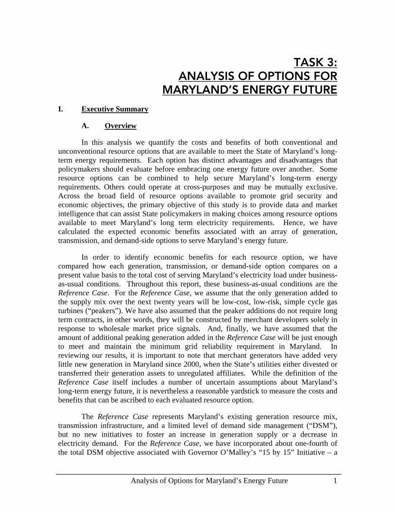
Maryland’s RPS is also embedded in the Reference Case and each Alternative Case. The availability of out-of-state Renewable Energy Credits (“RECs”), the relatively low current demand for RECs, uncertainties about the expiration of federal tax credits, and wind project siting issues, have created little incentive to date to build new renewable generation projects in Maryland. In the Reference Case and each Alternative Case, except wind, we have assumed that Maryland’s utilities and other load-serving entities will continue to be able to purchase out-of-state RECs to meet their non-solar RPS compliance requirements. The forecast of REC prices assumes increasing demand for RECs and gradual convergence of regional REC markets. For the Wind Case, we have credited the wind projects with the value of the RECs created. To comply with the solar band, in all cases we assume that sufficient 1 MW photovoltaic (“PV”) units will be installed on customer sites to meet the full requirement in all forecast years.
E. Financial Results – Wholesale
The financial model used for this study develops a total cost for generation services, including PJM transmission costs, the net effects of any contractual arrangements for solar or other generation, and the net effects of DSM initiatives. Figure 52 summarizes the total annual costs for the Reference Case. The bars representing the energy and capacity benefits of solar and DSM initiatives are below the x-axis, representing credits against total cost.

Analysis of Options for Maryland’s Energy Future 8
Figure E-1. Reference Case Annual Costs
(2,000)
0
2,000
4,000
6,000
8,000
10,000
12,000
14,000
16,000
2008
2010
2012
2014
2016
2018
2020
2022
2024
2026
Ann
ual C
ost (
$ M
illio
ns)
Solar EnergyMarket ValueSolar CapacityMarket ValueDSM ProgramCapacity SavingsDSM ProgramEnergy SavingsSolar ProgramDirect CostsDSM ProgramDirect CostsPJM TransmissionCostsUnadjusted MarketCapacity CostUnadjusted MarketEnergy CostTotal Cost
The present value of this series of annual costs for the Reference Case is about $73 billion, the baseline for determining EVA for each Alternative Case. Figure 85 shows the total present value for each of seven Alternate Cases.
Figure E-2. Present Value Cost Comparison by Case
70,76770,682 70,94873,28472,06772,955 72,759 70,041
(10,000)
0
10,000
20,000
30,000
40,000
50,000
60,000
70,000
80,000
Ref
eren
ce C
ase
Opt
imum
Mix
Cas
e
Coa
l Cas
e
Nuc
lear
Cas
e
15x1
5 D
SM C
ase
Tran
smis
sion
Cas
e
Win
d C
ase
1200
MW
CC
Cas
e
PV o
f Cos
t ($
Mill
ions
)
PPA Net EnergyMargin
PPA CapacityCredit
PPA Direct Costs
DSM ProgramCosts
PJM TransmissionCost
Market CapacityCost
Market EnergyCost
Total Cost

Analysis of Options for Maryland’s Energy Future 9
Figure E-3 shows the cumulative present value of net benefits for each of the seven Alternative Cases. The end point on the right-hand side for each case is the EVA.
Figure E-3. Cumulative Present Value
(500)
0
500
1,000
1,500
2,000
2,500
3,000
3,500
2008 2010 2012 2014 2016 2018 2020 2022 2024 2026
Cum
ulat
ive
Pres
ent V
alue
(EVA
, $ M
illio
ns)
Optimum Mix Case
Coal Case
Nuclear Case
15 by 15 DSM Case
Transmission Case
Wind Case
Overbuild Case
Four significant points emerge. First, the benefits associated with the 15 x 15 DSM Case materialize immediately and climb steadily over the study period. Second, even though no economic benefits arise under the Nuclear Case until 2017, the magnitude of the benefits is so large that the resulting EVA by far exceeds those associated with any other resource option. Third, like nuclear, no benefits accrue under the Transmission Case until 2015, but the magnitude of the benefits relative to Maryland’s utilities’ incremental costs are so large that the corresponding EVA is very high. Finally, the benefits associated with the Overbuild Case materialize once the 1200 MW capacity is built and accumulate steadily over the study period, yielding an EVA roughly the same as both the 15 x 15 DSM Case and the Transmission Case.
Figure E-4 and Figure E-5 show the EVA for each of the seven Alternative Cases and break down the costs and benefits separately, with benefits above the x-axis (the zero-line) and costs below the x-axis.

Analysis of Options for Maryland’s Energy Future 10
Figure E-4. EVA by Component – Generation Cases
196
2,007
2,914
888
(4,000)
(3,000)
(2,000)
(1,000)
0
1,000
2,000
3,000
4,000
5,000
6,000
7,000
Optimum Mix Case Coal Case Nuclear Case 1200 MW CC Case
Diff
eren
tial E
VA ($
Mill
ions
)
PPA Net Energy MarginPPA Capacity CreditPPA Direct CostsMarket Capacity CostMarket Energy CostTotal EVA
The Optimum Mix Case produces negligible savings attributable to lower energy prices for a brief interval after adding combined cycle generation. The Coal Case shows significant market energy and capacity benefits over the study horizon, but like the other capital-intensive, baseload options, utility ratepayers would have to assume the substantial “PPA Direct Costs” (yellow bar) shown below the x-axis. Such PPA Direct Costs would not be avoidable, that is, they would be incurred, for the most part, on a take-if-tendered basis. The Coal Case shows offsetting benefits from the net market value of the energy and capacity, yielding an EVA of $888 million. Like Coal, the Nuclear Case shows even higher direct payments to the supplier. Because of the low marginal cost of producing energy from a nuclear power plant, the PPA Net Energy Margin is very large. The project EVA of $2.9 billion for the Nuclear Case is driven primarily by the value of the PPA Net Energy Margin and, to a lesser extent, by the reduction in energy prices in Maryland, i.e., Market Energy Cost. The Overbuild Case produces a material reduction in market capacity prices and, to a lesser extent, energy prices. The EVA of the Overbuild Case is $2.0 billion. In interpreting the results of the Overbuild Case it should be noted that the PPA Direct Costs shown in yellow are so large because we have assumed that all peaker additions over the study horizon would likewise require long-term agreements once capacity and energy prices are reduced due to excess generation in SWMAAC.
It is useful to consider the relative magnitudes of the benefit-to-cost ratios for each of the aforementioned Alternative Cases. For each option, the benefits equal the height of the bar above the x-axis and the costs equal the height of the bar below the x-axis. For the Optimum Mix Case, there is no meaningful ratio to report as there are no direct costs shifted to ratepayers. For the Coal Case, the ratio is 1.7, largely a reflection of the long-term value of the “dark-spread” – the difference between the value of energy

Analysis of Options for Maryland’s Energy Future 11
in Maryland and the marginal cost of producing energy from a coal plant. For the Nuclear Case, the ratio is 2.1, also largely a reflection of the value of energy produced under the contract and the decreased energy prices during the second-half of the planning horizon. For the Overbuild Case, the ratio is only 1.4 because it would not be reasonable to anticipate continued merchant entry once both capacity and energy prices have been deflated.
Figure E-5 shows a similar breakdown for three non traditional Alternative Cases.
Figure E-5. EVA by Component – Non-Traditional Cases
2,273
(329)
2,188
(4,000)
(3,000)
(2,000)
(1,000)
0
1,000
2,000
3,000
4,000
5,000
6,000
15x15 DSM Case Transmission Case Wind Case
Diff
eren
tial E
VA ($
Mill
ions
)
PPA Net Energy MarginPPA Capacity CreditPPA Direct CostsDSM Program CostsPJM Transmission CostMarket Capacity CostMarket Energy CostTotal EVA
Although the 15 x 15 DSM Case produces an EVA of about $2.3 billion, it requires about $3 billion in DSM Program Costs. The reduction in energy and capacity prices includes both the lower prices that benefit all ratepayers and the avoided energy use that benefit only the direct participants. We have not estimated the economic value of any loss in consumer comfort or convenience. The benefit-to-cost ratio is 1.8.
The Transmission Case produces an EVA of about $2.2 billion. Despite the high cost of new highway transmission projects, Maryland’s share of the incremental PJM transmission charges is small, which results in a ratio is 21.4, by far the largest and most robust across the array of cases evaluated in this study.
The Wind Case produces an EVA of negative $329 million. When offshore and onshore wind are considered as one project, the benefit-to-cost ratio is 0.8, well short of the point of economic indifference. When the onshore portion is treated separately from the offshore portion, the EVA is slightly positive – about $78 million – compared to extremely negative for the offshore project, about negative $515 million. The

Analysis of Options for Maryland’s Energy Future 12
corresponding benefit-to-cost ratios for the onshore and offshore wind projects are 1.2 and 0.6, respectively.
F. Financial Results – Retail
Based on the load profiles for residential and commercial/industrial (“C&I”) customers provided by the Maryland utilities, we allocated the annual costs and benefits of each Alternative Case, relative to the Reference Case. We computed the percentage change in the power supply costs associated with the classes for each utility, relative to the Reference Case.
Figure E-6 shows the percentage change for Allegheny on a present value basis over the study period.
Figure E-6. Change in Allocated Power Supply Cost – Allegheny
-6%
-5%
-4%
-3%
-2%
-1%
0%
1%
2%
Res C&I I C&I II C&I III
Perc
ent C
hang
e in
Pow
er S
uppl
y C
ost (
PV) Optimum Mix
Coal
Nuclear
15 by 15 DSM
Transmission
Wind
Overbuild
Figure E-7 shows similar percentage changes for BGE. Because BGE’s load is located within SWMAAC, the generation cases (Coal, Nuclear, Overbuild) and the Transmission Case impact its rates more than APS or Delmarva.

Analysis of Options for Maryland’s Energy Future 13
Figure E-7. Change in Allocated Power Supply Cost – BGE
-6%
-5%
-4%
-3%
-2%
-1%
0%
1%
2%
Res C&I I C&I II C&I III
Perc
ent C
hang
e in
Pow
er S
uppl
y C
ost (
PV) Optimum Mix
Coal
Nuclear
15 by 15 DSM
Transmission
Wind
Overbuild
Figure E-8 shows the percentage changes in Delmarva’s power supply costs, which are similar to those for Allegheny, but differ in the effect of the Transmission Case, which is essentially neutral for Delmarva.
Figure E-8. Change in Allocated Power Supply Costs – Delmarva
-6%
-5%
-4%
-3%
-2%
-1%
0%
1%
2%
Res C&I I C&I II C&I III
Perc
ent C
hang
e in
Pow
er S
uppl
y C
ost (
PV) Optimum Mix
Coal
Nuclear
15 by 15 DSM
Transmission
Wind
Overbuild

Analysis of Options for Maryland’s Energy Future 14
Finally, Figure E-9 shows allocated retail power supply cost changes for PEPCO, which are very close to or identical to those for BGE.
Figure E-9. Change in Allocated Power Supply Costs – PEPCO
-6%
-5%
-4%
-3%
-2%
-1%
0%
1%
2%
Res C&I I C&I II C&I III
Perc
ent C
hang
e in
Pow
er S
uppl
y C
ost (
PV) Optimum Mix
Coal
Nuclear
15 by 15 DSM
Transmission
Wind
Overbuild
G. Conclusions
The study results suggest the following conclusions:
The delivered cost of natural gas and, to a lesser extent, the cost of residual fuel oil will greatly influence Maryland’s energy prices for the foreseeable future. These price variations create by far the most significant potential impacts on electric energy costs and are largely beyond Maryland’s control. So long as in-state generation is dependent on natural gas or oil to generate electricity, the State will be vulnerable to rising and largely uncontrollable costs.
Our quantitative analyses identify clear differences among several of the option scenarios. EVAs for the Transmission Case, Nuclear Case, and the DSM Case show the greatest promise. Relative to the Reference Case, each of these energy futures confers value ranging from $2.2 billion to $2.9 billion. Of course, each option also poses discernible risks. The State cannot completely control whether or when a beneficial transmission project will be sited, permitted, financed, and completed. A new nuclear plant may also encounter licensing, financing, design, or construction obstacles that may delay or prevent its operation. To the best of our knowledge, although other states have established similar ambitious targets, the aggressive DSM programs that will be necessary to achieve the target penetration levels have

Analysis of Options for Maryland’s Energy Future 15
not been implemented elsewhere on this scale. Moreover, the program costs associated with the market penetration rates underlying the forecast of benefits are highly uncertain.
Other analyzed options offer potential economic benefits but could create environmental and market detriments as well. The addition of 1200 MW of gas-fired capacity associated with the Overbuild Case can materially reduce Maryland’s energy and capacity charges, but it will not reduce reliance on natural gas, thereby exposing Maryland’s ratepayers to continued wholesale energy price volatility. Moreover, investment in a sustained MW overhang could undermine the goals of a workably competitive wholesale market before it is known for sure whether or not capacity price signals actually work. On a purely economic basis, a large, state-of-the-art coal plant could also reduce costs, but concerns about greenhouse gas emissions may preclude that alternative. Similarly, a new highway transmission project that increases Maryland’s ability to import cheaper electricity from the west may also raise environmental issues about reliance on generation that produces higher quantities of greenhouse gases from coal plants, i.e., “leakage.”
BGE’s and PEPCO’s ratepayers will likely realize most of the benefits from the analyzed options. APS’s service territory in western Maryland does not suffer from the same transmission constraints as SWMAAC and would, therefore, not receive benefits comparable to those identified for BGE, PEPCO, and, to a lesser extent, Delmarva. In some instances, APS may even be somewhat adversely impacted. At the retail level, the most promising resource options can potentially reduce the power supply portion of rates for BGE and PEPCO by as much as 5% relative to the Reference Case.
The State will need more intensive evaluation of the most attractive alternatives before it finalizes the best approach to meet long-term energy requirements. We recommend that policy makers assess the risks entailed in proceeding with each of the most promising options. Rigorous analysis is required before selecting the best mix of resource options that achieves reasonable tradeoffs between risk and reward.
II. Overview
A. Background and Purpose
Under Chapter 549, Maryland Laws of 2007, the General Assembly required the Public Service Commission (“PSC”) to evaluate the status of electric restructuring in Maryland and to assess options for re-regulation. To the extent that re-regulation is advisable, its goal would be to derive the most beneficial rates for customers while maintaining reliable electric service. The legislation requires the PSC to examine whether the State’s Investor Owned Utilities (“IOUs”) should be required to construct new plants and/or contract directly with generators for new supply. New supply options may include base, intermediate, and/or peaking generation, including renewable technologies. To facilitate the addition of new generation in Maryland, utilities may

Analysis of Options for Maryland’s Energy Future 16
enter into long-term contracts or, alternatively, own and operate generation added to the State’s resource mix.
To assist the PSC in complying with its statutory obligation, this report analyzes the impact on wholesale and retail electricity prices of potential policy, legislative, and regulatory initiatives that the PSC and/or the General Assembly may undertake to promote economic and energy security. Our analysis assesses the costs and benefits of incentives to develop different types of new generating resources in the State. We also emphasize the relative economic merit of new, high-voltage transmission projects designed to alleviate existing congestion patterns in Maryland. We consider effective measures to promote energy efficiency, conservation, and peak demand reduction – which Governor O’Malley has promoted to achieve a 15% reduction in per capita energy use by 2015 (hereafter referred to as the “15 by 15” Initiative) – among the range of potential options. We quantified price impacts of the various resource and ownership options using a suite of electric system and rate models that simulate the region’s wholesale and retail markets over the 20-year planning horizon from 2008 through 2027.
In Section II.D we describe the methodology and modeling framework employed to measure the relative costs and benefits. In Section III.C, we describe the costs and operating parameters for commercially available generation technologies that can provide base, intermediate, and peaking generation to serve Maryland’s electricity demand over a long-term planning horizon. We describe renewable technologies that have the potential to satisfy Maryland’s Renewable Portfolio Standard (“RPS”) under Senate Bill 595, including the new “solar band” requirement. In Section III.D we evaluate various energy efficiency, conservation, and demand-side management (“DSM”) programs that can potentially help Maryland achieve all or a portion of its “15 by 15” initiative.
We have quantified the costs and benefits that Maryland ratepayers may be able to achieve under an array of resource options and have delineated relevant wholesale and retail price effects, including environmental compliance costs, but not external effects.1 Economic results are presented in Section IV.D.
It is important to note that the economic and operational merit of certain resource options will be materially impacted by external events, policies, and market conditions beyond the State’s control. For example, siting of a new transmission project into Maryland or the addition of a new nuclear power plant to the State’s resource mix will be driven by factors that the State may facilitate and influence but cannot absolutely control. Consequently, throughout this report we have identified on a qualitative basis many of the external commercial and regulatory considerations associated with the promotion of new generation, transmission, or demand side resources to meet Maryland’s increased electricity requirements over the study horizon.
1 External environmental impacts such as health consequences, property devaluation, and the effects
of climate change are outside the scope of this analysis.

Analysis of Options for Maryland’s Energy Future 17
B. Modeling Framework
Our analysis of potential industry restructuring in Maryland begins with the development of an integrated suite of economic, mathematical, and production simulation models. We have relied on this modeling framework to test the impact of postulated technology, policy, and regulatory initiatives designed to ensure that electricity demand and supply in Maryland remain approximately in equilibrium over the 20-year study period. Figure 10 shows a schematic of the modeling framework. Our approach simulates wholesale energy markets in PJM over the long term when different resources are added by technology type in Maryland. Consistent with current market rules in PJM, we have differentiated energy and capacity prices by location over the study horizon. Working in cooperation with Maryland’s utilities, we have also estimated the long-term retail rate impact by class of service for each of the technology options examined in this study.

Analysis of Options for Maryland’s Energy Future 18
Figure 10. Study Framework
CaseDefinitions
Fuel Price Forecasts
ReliabilityCriteria
Loads by Zone
GenerationResources
TransmissionResources
Utility LoadData
Non-BypassableUtility Charges
Alternate CasesRetail Rates
Net Retail RateImpact by Case
Reference Case Alternate Future
Cases
Generation additionsTransmission additionsLoad modifications (DSM)
Inpu
tsM
arke
t Sim
ulat
ion
Energy Revenue
Entry/AttritionLMP’s by Zone
UCAP byLDA
PJMCharges
AlternateCases
Ret
ail A
naly
sis
Load Shape byCustomer Class
Transmission Limits
MarketSym RPM Ancillary Services
Utility RetailRate Models
Net WholesalePrice Impacts
Who
lesa
le M
arke
t Ana
lysi
s
Inpu
tsR
ate
Mod
el
ReferenceCase
Reference CaseRetail Rates
At the wholesale level, the key measurement for resource futures that we examined is the total cost to serve load. Quantification of the total cost to serve load encompasses all electricity load in Maryland, including the loads of municipal utilities and cooperatives. Likewise, we have also counted the retail loads of customers who “shop,” i.e., retail customers who have migrated to competitive suppliers. To the extent that a State initiative lowers or stabilizes market electricity prices, all Maryland customers would benefit, including customers of municipals and cooperatives. In order to keep this analysis from becoming unwieldy, we have made the simplifying assumption that direct program costs are non-bypassable and are allocated fully only to Baltimore Gas & Electric (“BGE”), Delmarva Power & Light (“Delmarva”), Allegheny Power

Analysis of Options for Maryland’s Energy Future 19
System (“APS”), and Potomac Electric Power Company (“PEPCO”). We estimate retail rate impacts for each IOU doing business in Maryland.
Working in association with the PSC, we have hypothesized a number of alternative resource futures to meet Maryland’s long-term energy requirements. Each resource option is technologically feasible and, therefore, can diversify Maryland’s energy infrastructure, thereby enhancing reliability and economic benefits. Certain of these alternative resource futures are mutually exclusive, others are not. To derive the economic benefits and costs associated with alternative energy futures, we have compared the economic impact of each alternative resource future to a baseline estimate of Maryland’s total cost to serve load under status quo market and operating conditions. Formulation of the status quo is the yardstick for comparison. Definition of the status quo over the study horizon is the Reference Case – the benchmark against which we gauged the net benefits or costs of each distinguishable resource future. Hence, the Reference Case is a postulated “business-as-usual” condition representing Maryland’s resource mix, transmission infrastructure, and DSM regime in the absence of new initiatives to foster the addition of new generation, transmission, or DSM initiatives that would be necessary to meet the Governor’s “15 by 15” goal.
In the Reference Case, our starting point for quantifying the net benefits attributable to alternative resource options is a long-term competitive equilibrium where there are no unserved energy requirements over the study horizon. As load grows, we have assumed the addition of simple cycle peakers to ensure resource adequacy objectives without explicitly considering what payments from Maryland’s utilities may be required to ensure the addition of these peakers when and where they are needed. The simple cycle peaker is a gas turbine (“GT”) that is the lowest cost resource addition that maintains grid reliability. Despite the near absence of significant new generation resources added to Maryland’s supply mix since 1999, the Reference Case assumes that Maryland will not tolerate brown outs or blackouts over the study period. Other operational criteria to safeguard against the potential loss of generation or transmission infrastructure in PJM – first order and second order contingencies – have been treated consistently with existing PJM and North American Electric Reliability Corporation reliability criteria.
The addition of GTs may not constitute the “optimal” resource addition to meet Maryland’s load growth. Nevertheless, we have postulated GTs because they are the quickest to site and construct, least expensive in terms of capital cost, and lowest risk in terms of assurance of reliability. Therefore, the Reference Case represents the resource expansion path that constitutes minimum adequate supply. The Reference Case does not include generation or transmission projects that have not been built – or that may never be built – due to permitting challenges, uncertainties in the capital markets, or wholesale market dynamics that impair new entry. The following resource options have not been included in the Reference Case: high voltage, transmission “highway” projects, combined-cycle plants, new coal plants, new in-State renewable energy resources, in particular, wind, or a new nuclear plant. The Reference Case does, however, assume a modest penetration of demand-side resources, corresponding to about 25% of the “15 by

Analysis of Options for Maryland’s Energy Future 20
15” Initiative. The Reference Case also assumes that each of the Maryland utilities complies with Maryland’s RPS. Details of the Reference Case are presented in Section B.
The Reference Case culminates in a benchmark forecast of location-based wholesale energy and capacity prices for Maryland over the 20-year study horizon. This period is sufficient to capture the first-order price effects ascribable to alternative resource expansion plans, including retail ratepayer impacts. We considered extending the study horizon beyond twenty years, but rejected that approach because it would entail unavoidable uncertainty associated with longer forecast periods. Importantly, the Reference Case forecast incorporates the expected value for external variables that are largely or exclusively outside the Commission’s control, including the cost of fuel delivered to power plants in Maryland and the PJM Interconnection (“PJM”) at large, load growth throughout the region as well as in neighboring market areas, environmental standards, the location and timing of liquefied natural gas (“LNG”) import terminals along the Atlantic seaboard, expansion of interstate pipelines and underground storage facilities, Nuclear Regulatory Commission (“NRC”) license extensions and approvals, as well as other economic and financial parameters.
Against the Reference Case, we compare seven different alternative cases that span a range of potentially feasible generation additions, transmission expansions, and load management options that the State may effectuate through different policy decisions or regulatory actions. These cases are as follows:
Optimum Mix Case – Whereas the Reference Case postulates only the addition of the lowest capital cost resource additions, the Optimal Mix Case consists of an aggregate of gas-fired combined cycle and gas turbine technologies that could arise from rational merchant investment in new generation in Maryland. Although combined cycle plants have materially higher capital costs, they operate at a lower heat rate and can garner higher energy revenues, thereby justifying the investment, if the capacity factor is sufficiently high.
Coal Case – This case assumes the construction of a new, supercritical
pulverized coal plant with state-of-the art environmental controls located in Maryland. The plant could be the centerpiece of a “reregulation” initiative that directs the utilities either to own the asset directly or enter into a long-term contract with a developer. We assume that the plant would achieve commercial operation in 2015.
Nuclear Case – Constellation recently filed a partial application to construct a
third reactor unit at its Calvert Cliffs facility and that the installed capacity of the new nuclear unit is 1,600 MW. We assume that this facility would be operational in 2017. Finally, we have assumed that the utilities would enter into a long-term contract with Constellation for the entire output of the plant.

Analysis of Options for Maryland’s Energy Future 21
15 by 15 DSM Case – In this case, we evaluate the costs and benefits of fully achieving the 15 by 15 DSM goal in Maryland through utility-sponsored initiatives, regulatory mandates, and voluntary ratepayer actions.
Transmission Case – Several backbone transmission projects have been
proposed in PJM to alleviate congestion and promote system reliability. In this case, we assume that one of these major projects – the 502 Junction to Loudoun transmission project – will be constructed and placed in service by 2015. The costs for this project would be allocated in accordance with Federal Energy Regulatory Commission (“FERC”)-approved market rules applicable to high voltage transmission projects.
Wind Case – Maryland’s RPS is intended to promote the construction of new
renewable resources within the State. In this case, we assume that 500 MW of new wind turbines are installed in the State between 2008 through 2012 (200 MW inland plus 300 MW offshore). These projects would be sponsored by developers but supported through long-term contracts with the utilities.
Overbuild Case – In this case, we assume that over the study period,
Maryland maintains approximately 1,200 MW of surplus generating capacity in the form of new gas-fired generation projects in the Southwest Mid-Atlantic Area Council (“SWMAAC”) Locational Delivery Area (“LDA”). In order to maintain this generation surplus, we assume that Maryland’s utilities would enter into long term contracts to ensure that the supplier(s) realize a reasonable return on investment. This case is tantamount to a sustained “megawatt overhang” in relation to the target reserve margin defined by PJM. We evaluated the market impact of the MW overhang in SWMAAC and the associated costs to ratepayers.
For each case, we modeled the impact of the resource additions on wholesale energy and capacity prices in Maryland over the 20-year forecast horizon. For each year, we also calculated the direct and indirect costs to load in the form of contract obligations or DSM program costs. Section IV.C provides details on how we constructed each case and the underlying assumptions.
The difference in the cost to serve Maryland’s load between the Reference Case and each alternative resource case represents the aggregated net benefit or cost of the postulated resource or policy option. We calculated the present value of this net benefit or cost over the study horizon. The present value of the net benefit or cost in relation to the total cost to serve load in the Reference Case is expressed in terms of Economic Value Added (“EVA”). EVA therefore represents a Mark-to-Market (“MTM”) accounting of the change in cost to serve load in Maryland under the wholesale market prices simulated for each resource option versus the Reference Case. We also evaluated ratepayer impacts for each resource, ownership, and regulatory option considered in this study.

Analysis of Options for Maryland’s Energy Future 22
Retail rate impacts for each resource option reflect the net change in energy costs across different customer classes, as well as the direct costs to implement the option. To calibrate the change in retail rates by utility and customer class, we have included the expected cost to implement the option, e.g., system benefits charges, increases in transmission and distribution charges, customer rebates, or, in the case of DSM, direct customer expenditures for energy-efficient appliances. Hence, our analysis evaluated the average impact to a typical monthly bill for each utility and each customer class. Within each customer class, we have not attempted to differentiate among customers who choose to participate in certain programs and those who do not.
C. External Conditions and Variables
Many external conditions are largely outside the State’s ability to control. Wholesale electric market rules administered by PJM are FERC jurisdictional and are, therefore, largely beyond the State’s authority. Market dynamics affecting fuel prices delivered to power plants throughout PJM are also largely unaffected by state actions. In this section, we address many of the external variables and assumptions incorporated in the Reference Case and each of the alternative cases. These external variables and key factor inputs to our mathematical, financial, and simulation models determine the wholesale energy and capacity prices over the study horizon.
1. Fuel Price Outlook
The delivered cost of fuel to power plants throughout PJM is the single largest determinant of electric energy prices. Whereas global market forces set the price of oil, market dynamics across North America have the greatest impact on the price of natural gas. Although oil is not a primary fuel for electricity production in Maryland, it is still a critical fuel with respect to bulk power security throughout the heating season, November through March. The relationship between oil and natural gas also has a direct bearing on energy prices throughout the region – there has been an historic linkage between the price of oil and natural gas. In SWMAAC and the Eastern Mid-Atlantic Area Council (“EMAAC”) LDA, the delivered cost of natural gas often sets the market clearing price of electric energy, sometimes even when natural gas is not the marginal fuel. Thus, charting the complex, interaction effect between oil and natural gas is an integral part of the long-term forecast of fuel prices delivered to power plants in PJM and the resulting electric energy prices in Maryland.
Over the last two decades, the price of natural gas was determined largely by continental and regional forces. That dynamic is beginning to change as global competition for LNG exposes LNG import terminals along the Atlantic seaboard to market pressures on both sides of the Atlantic Ocean, and, to a lesser extent, in the Pacific Rim as well. Consequently, the delivered cost of LNG, a primary fuel affecting natural gas prices in SWMAAC and EMAAC, is beginning to reflect global rather than continental pricing pressures. Coal is another primary fuel of critical relevance in setting energy prices in PJM. Coal prices are largely determined by regional market dynamics. Finally, the price of uranium, another global commodity, is a primary fuel input for

Analysis of Options for Maryland’s Energy Future 23
electricity generation in PJM. Because nuclear power plants throughout PJM are considered price takers, not price setters, uranium prices have little to do with setting electric energy prices in PJM. In this section, we review the market fundamentals affecting the price of fuels for electricity production in PJM, emphasizing the building block assumptions underlying our Base Case forecast of fuel prices that support the analysis of technology options.
The forecasted prices of natural gas, oil, coal, and uranium are subject to a broad range of uncertainties regarding resource availability and depletion, environmental factors, weather, geopolitical events, as well as supply/demand fundamentals in global, continental and regional energy markets. Oil and gas prices have demonstrated extremely high price volatility over the last decade, in particular, over the last two years. This trend is likely to continue over the 20-year study horizon in response to robust global demand for transportation fuels, e.g., strong demand in China and India. Skyrocketing fossil fuel prices have also indirectly helped to sustain upward pressure on uranium prices, which have recently run-up after over two decades of price stability. To account for uncertainty, we have developed high and low fuel price forecasts in order to define upper and lower limits on electric energy prices over the study horizon. Whereas the high fuel price forecast represents a plausible upper limit on premium fossil fuel prices, the low fuel price forecast is not intended to represent a plausible lower limit on fossil fuel prices. In other words, the low fuel price alternative case is not realistic given current market pressures and trends. We formulated the trajectory of low oil and gas prices merely to demonstrate the linkage between low fuel prices and wholesale electricity prices in Maryland.
The high and low alternate cases assume distinctly different perspectives on the oil and natural gas resource base, e.g., the effects of maturing development and depletion trends on long-term oil and gas production, as well as different demand trajectories over the forecast horizon. We completed the fuel price forecasts developed for this analysis in August 2007, using a 2007 Q3 market outlook. We used the Base Case forecast to analyze supply and demand options to meet Maryland’s long-term energy needs, but in evaluating the forecast of long-term energy prices, we considered the Peak Oil Case and the Low Case.
(a) Base Case Forecast
Increased demand for electricity throughout the developing world as well as in the U.S., Europe, and Japan is likely to sustain a tight balance between the supply and demand for primary generation fuels. Low supply elasticities in the amount of oil and natural gas available in global markets in response to high commodity prices will likely sustain upward price pressure over the study horizon. Traditionally, there has been a relatively high correlation between crude oil prices and natural gas prices. Recently, the historic linkage between oil and natural gas has materially weakened, however, in response to heightened production pressures on the Organization of the Petroleum Exporting Countries (“OPEC”) and non-OPEC producers to keep pace with the world’s demand for transportation fuels. Global oil reserves may be approaching production

Analysis of Options for Maryland’s Energy Future 24
limits, causing oil production levels to peak. Whereas oil reserves are located primarily in the Middle East, Venezuela, Africa and Russia, natural gas reserves are more widely distributed.
With the U.S. dependent on oil imports for more than 60% of demand, oil prices are driven by geopolitical and resource related developments throughout the Middle East, Venezuela, the Former Soviet Union (“FSU”), and, to a much lesser extent, both Canada and Mexico. In contrast, the natural gas market is largely a continental market – domestic production accounts for about 80% of U.S. consumption. Most of the remaining gas use is satisfied through supplies originating from western Canada. LNG imported from Trinidad and Africa currently provides only about 3% of total U.S. gas demand, but is forecast to increase significantly over the next 20 years in response to accelerated gas resource depletion in the Gulf Coast, Alberta, and many other conventional natural gas producing basins in the U.S.
The Base Case forecast constitutes the most likely or expected outlook over the study horizon. We assume growth in global consumption at near long-term historical rates, steady investment in global exploration and production, gradual development of alternative fuels such as ethanol, oil sands, gas-to-liquids and coal-to-liquids, continuing long-term global economic growth over the forecast period, and the expansion and addition of LNG terminals along the Gulf Coast, Atlantic Seaboard, eastern Canada, and Mexico. We also contemplate continued geopolitical tensions in the Middle East, Nigeria, and Venezuela over the long term, but we have not factored in the disruptive effect of a sustained loss in major oil production from exporting countries. Before addressing the market fundamentals for each primary fuel, Figure 11 shows a summary of average prices.

Analysis of Options for Maryland’s Energy Future 25
Figure 11. Fuel Price Forecast – Annual Average Prices (Nominal $/MMBtu)
0
5
10
15
20
25
30
2008 2010 2012 2014 2016 2018 2020 2022 2024 2026
Fuel
Pric
e ($
/MM
Btu
)Henry Hub Gas No. 2 Distillate Oil0.3% Sulfur Residual Oil Nuclear FuelNorthern Appalachian Coal
i) Oil
The forecasted price of crude oil is pegged to the price of West Texas Intermediate (“WTI”) oil, the benchmark crude for trade in the U.S. Refined petroleum product prices are highly correlated to the price of crude oil. The price forecasts for both distillate oil and residual fuel oil are based on the statistical relationship between each product and WTI. The primary pricing point for the refined products is New York Harbor. We adjusted basis differentials from the New York Harbor price to reflect transportation costs and local market conditions for regional fuel prices in SWMAAC and EMAAC.
We generated the crude oil price forecast using a Levitan & Associates, Inc. (“LAI”) econometric model that considers the relationship among crude oil prices and world oil demand, proved oil reserves, and OPEC production. OPEC production is one key parameter. The primary driver for crude oil prices, however, continues to be the growth in the global demand for refined transportation fuels. The Base Case outlook assumes that global trends will continue to reflect tight market fundamentals over the 20-year study horizon. We see global oil demand increasing at an annual rate of about 2% through 2012. This near term outlook on worldwide demand is consistent with the recent forecast provided by the International Energy Agency (“IEA”).2 After 2012, oil demand in China and India is expected to slow to a more sustainable long-term trend relative to the explosive growth rates observed in both countries since 2000. From 2012 to 2015, 2 International Energy Agency, Medium-Term Oil Market Report, July 2007.

Analysis of Options for Maryland’s Energy Future 26
the annual growth rate in oil demand decreases to around 0.5% in response to high prices. After 2015, we anticipate a return to a long-term annual growth rate of approximately 1.25% for the remainder of the forecast period. We have assumed that world oil consumption will grow from 84.5 million barrels per day in 2006 to 114.7 million barrels per day by 2028. OPEC production is assumed to increase from around 30 million barrels per day in 2007 to 52 million barrels per day in 2028, based on IEA’s analysis of medium-term OPEC production capacity and the U.S. Energy Information Administration’s (“EIA”) long-term forecast of OPEC production.3 We base our assumptions regarding global proved reserves on a review of long-term historical trends in reserve growth. We have also considered the recent decline in reserves that occurred over the last two years. In our forecast, global reserves are expected to continue to increase, but at a gradually diminishing rate, increasing from 1,208 billion barrels in 2006 to 1,430 billion barrels in 2028.
The Base Case encompasses a significant price elasticity of demand. We expect the worldwide demand for transportation fuels to be tempered in response to high prices. We also assume that additional oil supplies will be available from other conventional and unconventional resources, albeit at higher cost, including growing production from the oil sands deposits in Alberta, new fields in the former Soviet Union, Arctic developments, and in the deep water of the Gulf of Mexico. There are also promising supply fundamentals offshore Brazil. As shown in Figure 12, we expect oil prices to peak in 2012 at $93/Bbl. After declining significantly in real terms from 2012 through the middle of the next decade, we expect oil prices to increase significantly over the duration of the study horizon, reaching $128/Bbl in 2028.
3 U.S. Energy Information Administration, 2007 International Energy Outlook.

Analysis of Options for Maryland’s Energy Future 27
Figure 12. Base Case WTI Forecast (Nominal $/Barrel)
0
30
60
90
120
150
2008 2010 2012 2014 2016 2018 2020 2022 2024 2026 2028
Oil
Pric
e ($
/Bbl
)
Figure 13 provides the forecasts of prices for No. 2 fuel oil, and 0.3% and 0.5% residual fuel oil at New York Harbor. The prices for fuel oil delivered to electric generators in SWMAAC and EMAAC incorporate a basis of approximately $1.75/Bbl.

Analysis of Options for Maryland’s Energy Future 28
Figure 13. Fuel Oil Price Forecasts (Nominal $/MMBtu)
0
5
10
15
20
25
30
35
2008 2010 2012 2014 2016 2018 2020 2022 2024 2026 2028
Oil
Pric
e - D
eliv
ered
($/M
Mbt
u)No. 2 0.3% 0.5%
ii) Natural Gas
The most important gas-producing regions in North America are the Gulf Coast, which includes the onshore Gulf Coast and the offshore Gulf of Mexico, the Western Canada Sedimentary Basin (“WCSB”), and the Rocky Mountains.4 Together these supply areas account for almost two-thirds of the total gas production in North America. The Gulf Coast provides more than half of total U.S. gas production. The WCSB accounts for the bulk of Canadian gas production and is the source for the almost all U.S. gas imports. The Rocky Mountains producing basins represent the largest supply sources in the U.S. with growing production and reserves.
Gas production throughout North America has not been highly elastic in response to high commodity prices over the recent historic period. Producers’ supply response has been limited, reflecting the accelerated depletion effect in the Gulf Coast and western Canada, as well as in conventional producing basins in Texas, onshore Louisiana, Oklahoma, Kansas, California, and, to a lesser extent, New Mexico. From a supply standpoint, production from the Rocky Mountains, the Barnett Shale in Texas, and in deep water in the Gulf of Mexico have been bright spots with respect to U.S. production.
4 For the purposes of this forecast, the Gulf Coast Onshore production includes production from the
states of Alabama, Louisiana, Mississippi, and Texas. The WCSB includes production from Alberta, Saskatchewan, and British Columbia. The Rocky Mountain supply region includes production from Wyoming, Montana, Utah, and Colorado.

Analysis of Options for Maryland’s Energy Future 29
Production from the Gulf Coast, particularly the offshore continental shelf, has been declining for several years, while WCSB production has essentially leveled off. Gas demand in Canada has increased, particularly from the highly gas intensive oil sands production which continues to ramp up in response to high oil prices. Natural gas producers have drilled more wells in response to high prices, but production has not increased accordingly. Depletion trends, pipeline transportation and storage constraints during the heating season, disappointing exploration results from Atlantic Canada, and growing gas demand for electricity generation have helped to sustain upward pressure on delivered natural gas prices at key pricing points in PJM. Throughout the U.S., robust electricity demand coupled with the environmental urgency associated with emissions of ozone precursors and greenhouse gases has made natural gas the fuel of choice for new power plants. Strong continental demand over the forecast period, coupled with weakening supply fundamentals, portends a growing natural gas supply gap. We expect this hydrocarbon gap to be filled through increased reliance on LNG.
We base our forecast natural gas prices – both into-the-pipe in major production areas and delivered to relevant market areas – on an analysis of continental market conditions. Our analytical approach uses the Gas Pipeline Competition Model (“GPCM”) system, a linear programming model that captures the supply chain across North America as well as regional market demand indices.5 GPCM incorporates a proprietary database, GPCMdat. GPCM provides a consistent means for determining the impact on regional gas prices associated with changes in gas production at basins throughout North America, demand changes, and infrastructure changes, particularly new or expanded LNG import terminals across North America. Where necessary, we have exercised professional judgment in making adjustments to the GPCMdat inputs.6 Appendix 1 provides additional information about GPCM.
Figure 14 presents our forecast of U.S. gas production and consumption through 2028.
5 LAI licenses GPCM from RBAC, Inc., a California software firm. 6 Data to support LAI’s inputs are from EIA, the National Energy Board of Canada, Natural
Resources Canada, Canadian Association of Petroleum Producers, the National Petroleum Council, as well as industry participants. The crude oil price forecast has been incorporated in GPCM.

Analysis of Options for Maryland’s Energy Future 30
Figure 14. Long-Term Forecast of U.S. Gas Production and Consumption
0
5
10
15
20
25
30
2008 2010 2012 2014 2016 2018 2020 2022 2024 2026 2028
Nat
ural
Gas
Pro
duct
ion
/ Con
sum
ptio
n (T
cf)
U.S. Production U.S. Consumption
For over thirty years, the U.S. has been dependent on Canada for natural gas imports. The outlook for Canadian production over the long term does not allow the U.S. to rely on Canadian imports from traditional production basins to supplant the decline in U.S. production. Increasing LNG imports will be necessary to meet the growing gap between consumption and production over the forecast period. As of August 2007, five LNG import terminals operate in the U.S. We anticipate that two of these LNG facilities will be expanded in the next few years. The forecast also includes the addition of 12 LNG import terminals in North America over the planning horizon. By 2017, when the last of the new LNG terminals comes on line, total North American LNG import capacity will exceed 24 Bcf/day.
Dominion’s Cove Point LNG terminal is undergoing a major expansion. Total storage capacity is being increased from 7.8 Bcf to 14.5 Bcf. Daily vaporization capacity will increase from 1.0 Bcf/day to 1.8 Bcf/day. These changes to total deliverability are scheduled to be commercialized in 2008. The large increase in daily sendout capability as well as storage capacity will provide the region with substantial increased deliverability through existing pipeline conduits that link the Cove Point terminal with the storage fields in Leidy, PA. The expansion of Cove Point, along with related expansions in regional pipeline and storage capacity, will increase the availability of natural gas for power generation in PJM.
North American production is undergoing a transition from production centered in traditional fields in Texas, Louisiana, Kansas, Oklahoma, the plains of eastern Alberta, and the shallow waters of the Gulf of Mexico to new production areas. These new

Analysis of Options for Maryland’s Energy Future 31
production areas include the deep water of the Gulf of Mexico, the Rocky Mountains, western Alberta, and British Columbia. Much of this new production will be sourced from unconventional reservoirs.7 As unconventional gas production increases, gas from these sources will account for almost one-half of total U.S. production before the end of the forecast horizon. Typically, production from many of these unconventional formations requires more expensive drilling and completion technologies to produce gas in marketable quantities.8
The primary driver for the development of unconventional gas has been the maturation of the North American gas resource base. The maturation effect means that fewer reserves and less production will be realized in response to increases in the rig count and total exploration and production spending. The maturing resource base also means that the long-term floor for gas prices – set by the marginal cost of production – will likely rise. Outside North America, gas production in Africa, the former Soviet Union, and the Middle East involve resources in comparative infancy. The large and generally untapped resources in these areas offer great promise for global LNG trade over the study horizon.
In Figure 15, we show natural gas price forecasts for Henry Hub and two regional pricing points relevant for PJM – DTI South Point (“DTI-SP”) and Transco Zone 6 Non-New York (“TZ6NNY”).9
7 Unconventional reservoirs include tight sands, coalbed methane, and shale gas that require
enhanced completion and production techniques. Production from unconventional reservoirs tends to be more expensive than production from conventional reservoirs.
8 Coalbed methane occurs within the fractures or cleat system of the coal, in many cases in conjunction with water, and requires extensive dewatering and fracturing before commercial production.
9 A third pricing point of relevance in PJM, Texas Eastern Transmission Company M3 Zone (“Tetco M3”), has not been included.

Analysis of Options for Maryland’s Energy Future 32
Figure 15. Long Term Forecast of Natural Gas Prices at the Henry Hub and PJM
0
2
4
6
8
10
12
14
16
18
20
2008 2010 2012 2014 2016 2018 2020 2022 2024 2026 2028 2030
Gas
Pric
e ($
/MM
Btu
)Henry Hub TZ6NNY DTI-SP
In nominal terms, gas prices at the Henry Hub will increase from an annual average of about $8.00/MMBtu to nearly $15.00/MMBtu in 2028.10 Transportation basis to the market area also increases significantly over the study horizon.
iii) Coal
Using LAI econometric models, we developed a forecast of coal prices differentiated by production basin for Central Appalachian Basin (“CAPP”), Northern Appalachian Basin (“NAPP”), and Powder River Basin (“PRB”). The explanatory variables incorporated in the models include the historical relationships among coal prices in the supply regions, mining productivity, natural gas prices, regional production, and the growing use of flue gas desulphurization (“FGD”). Delivery to PJM from these basins will add on the average $6/ton ($0.23/MMBtu) to NAPP prices, $12/ton ($0.50/MMBtu) for CAPP prices, and $29/ton ($1.65/MMBtu) for PRB coal.
Production costs and regional mining conditions greatly impact coal market prices. Underground mining productivity is the key factor affecting production costs in CAPP and NAPP, and underground mines account for about 65% of the coal produced in these regions. Underground production is expected to increase market share over the forecast horizon as Appalachian surface mines are depleted and surface mining declines in response to environmental protection standards. By comparison, PRB production 10 The implicit run-up in basis toward the back end of the forecast period is explained by the lack of
pipeline or storage infrastructure added to the gas-side resource mix over the planning horizon. Optimization of basis adders by location in PJM over the study horizon is outside the scope of this study.

Analysis of Options for Maryland’s Energy Future 33
involves surface mining of thick coal seams with relatively thin overburden, which is conducive to high productivity and resulting lower basin prices.
Contracts with end-users, primarily electric generators, cover 70% of the coal mined in CAPP, 80% of the coal mined in NAPP, and 80% of the coal mined in the PRB. Remaining coal purchases are transacted in the spot market, which are more volatile than contract prices and can influence contract prices – in some cases, serving as the benchmark for the initial price levels in new contracts or for restructured contracts. Contract prices do not always fully follow the movements in spot prices, however. During the recent spike in spot prices many large coal users refused contracts tied directly to spot prices. Hence, our forecasts of basin prices reflect the combination of both spot and contract prices.
Figure 16 compares the coal price forecasts developed for each supply basin. The forecasts reflect declining or relatively flat productivity in all of the supply basins as environmental regulations and depletion affect mining operations. These effects are likely to be most significant in CAPP, where surface mining is limited by the prohibition on mountain top removal techniques, and declining reserves reduce the availability and access to reserve blocks large enough to justify high productivity longwall mining.
Figure 16. Forecast of Coal Prices by Supply Basin
0
10
20
30
40
50
60
70
80
90
2008 2010 2012 2014 2016 2018 2020 2022 2024 2026 2028
Coa
l Pric
e (N
omin
al $
/Ton
)
CAPP NAPP PRB
iv) Nuclear Fuel
Our forecast of nuclear fuel prices is driven in part by uranium prices, which, over the forecast horizon, contribute on average about half of the total cost of nuclear fuel.

Analysis of Options for Maryland’s Energy Future 34
Nuclear fuel costs also include the costs of conversion (5%), enrichment (29%) and fabrication (12%).11 U.S. uranium prices declined from around $40/lb in the late 1970s to a range of $10/lb to $20/lb for most of the last twenty years. Recently, spot prices have soared. Spot uranium prices have exceeded $125/lb. The current long-term contract price is around $95/lb. By early August 2007, the spot price had eased to $90/lb. In our forecast, average annual uranium prices peak in 2007 and remain high through 2009. In 2010 prices decline sharply to $57/lb and continue to decline through 2012 in response to additional supplies coming into the market, primarily from new and expanded mining capacity at Cigar Lake and McArthur River in Canada, Olympic Dam in Australia, as well as several new mines in Kazakhstan.12 After 2012, we forecast price increases to average 3.5% to 4% annually for the remainder of the forecast horizon, driven by the growth in demand for fuel at domestic plants that have gradually expanded and are operating at higher capacity factors, and for new nuclear plants that are being built outside of the U.S. and Western Europe.
Figure 17 shows our forecast of nuclear fuel prices. The 2007 IEA forecasts that global nuclear generation will increase at an average annual rate of 1.3% and nuclear generation capacity will increase by about 100 GW by 2028. The largest increases in capacity are expected in China, India, and Russia.
11 Nuclear fuel supplies include mined and enriched U3O8, utility stockpiles of uranium, and
secondary sources such as recycled spent fuel and recycled weapons grade uranium and plutonium.
12 Cigar Lake, projected to produce about 15% of global mined uranium supplies was scheduled to go into commercial production in 2008. However, flooding at the project will delay commercial production for at least two years.

Analysis of Options for Maryland’s Energy Future 35
Figure 17. Nuclear Fuel Price Forecast
0
0.2
0.4
0.6
0.8
1
1.2
2006 2008 2010 2012 2014 2016 2018 2020 2022 2024 2026 2028
Nuc
lear
Fue
l Pric
e ($
/MM
Btu
)
(b) Sensitivity Cases
Market analyses in SWMAAC and EMAAC show the strong linkage between delivered natural gas prices and wholesale electric prices. Using our chronological model, MarketSym, we have simulated the change in wholesale electricity prices in Maryland when we use either the Peak Oil Case or Low Case fuel price outlook in lieu of the Base Case.13 Of critical importance, the Peak Oil Case represents a plausible upside bandwidth in prospective oil and natural gas prices over the planning horizon in light of geopolitical tensions, depletion trends, the high cost of accessing oil and natural gas in ultra-deepwater, heightened global competition for LNG, environmental regulations, and technology substitution effects, among other things. Although the oil and natural gas prices embedded in the Low Price Case over the first half of the forecast period comprise a plausible lower limit on premium fossil fuel prices, the price forecast over the second half of the planning horizon is merely indicative.14
We have illustrated each of the fuel forecast cases as a smooth, long-term trend, but actual fuel prices are certain to be volatile around the annual price trends charted as mean values in each sensitivity case. For simplicity sake, we have not incorporated 13 Other potential application(s) of the Peak Oil Case and Low Price Case are not part of the scope of
work covered in this study. 14 The long-term sustained decline in oil and natural gas prices over the second half of the study
period constitutes an extremely low probability outcome, but is nonetheless useful in testing the impact of low fuel prices on wholesale electricity prices.

Analysis of Options for Maryland’s Energy Future 36
adjustments to coal and nuclear fuel prices in the Peak Oil Case and the Low Price Case.15
i) Peak Oil Case
Strong global demand growth through 2015 in response to bullish macroeconomic factors, including continued robust demand in China and India, explains the Peak Oil Case, which is predicated on continued long-term supply pressures on world oil supply. The supply dynamic associated with the peak in global oil production is often referred to as the Hubbert’s Peak Scenario.16 Eventually, the price induced elasticity of demand tempers the global appetite for premium transportation fuels. In this case, we see demand growth slowing after 2015, reaching its apex in 2020, and declining for the remainder of the forecast period.
In the Peak Oil Case we contemplate the peaking of proved global reserves at 1,225 billion barrels from 2010 to 2015, followed by continued decline to 1,102 billion barrels by 2028. A peak in global oil production would also occur during this period. Underlying the higher than expected run-up in global prices is the impact of accelerated depletion at existing fields in the Middle East, coupled with the technical challenges experienced by oil producers in an effort to replenish declining reserves through new discoveries outside the Middle East. In the Peak Oil Case, global reserves decline faster than new reserves can be discovered and developed. In addition, new discoveries are not only more costly, but also produce smaller reserve additions for each new well drilled and completed
In the Peak Oil Case, OPEC struggles to grow production over the forecast period. Total OPEC production reaches 40 million barrels per day in 2028. This forecast also contemplates the intensification of geopolitical uncertainty in the Middle East that reduces production, limited access for new drilling, and technology setbacks regarding the timing and feasibility of substitute transportation fuels. Prices increase rapidly reaching $143/Bbl by 2020. After 2020, price elasticity impacts result in a decline in demand followed by a decline in oil prices with prices converging toward the Base Case price of $128/Bbl by 2028. Figure 18 shows the forecast of WTI in the Peak Oil Case (referenced as a solid blue line) compared to the Base Case.
15 In actuality, both coal and nuclear fuel prices would be impacted by high v. low oil and natural gas
prices, but the comparative impact on Location Marginal Prices (“LMPs”) in Maryland, in particular, and SWMAAC, in general, is minor.
16 M.K. Hubbert, a geophysicist for Shell Oil in the 1960s, developed a statistical approach to predicting the peaks in oil production for individual fields and supply basins. This approach was used to predict the peaking of and subsequent decline in U.S. oil production in the early 1970s. Over the years many experts have disagreed with Hubbert’s conclusions. Current “Hubbert’s Peak” advocates argue that world oil production is at or rapidly approaching its peak.

Analysis of Options for Maryland’s Energy Future 37
Figure 18. Peak Oil Case – WTI Forecast
0
30
60
90
120
150
2008 2010 2012 2014 2016 2018 2020 2022 2024 2026 2028
Oil
Pric
e ($
/Bbl
)
Peak Oil Case Base Case
Consistent with the econometrics employed in the Base Case, prices for distillate and residual products follow similar paths as the WTI price.
For the natural gas forecast under the Peak Oil Case, we assumed a similar development of new LNG import terminals as in the Base Case. As shown in Figure 19, however, the high price of oil has a significant upward impact on natural gas prices.

Analysis of Options for Maryland’s Energy Future 38
Figure 19. Natural Gas Forecast – Peak Oil Case
0
2
4
6
8
10
12
14
16
18
20
2008 2010 2012 2014 2016 2018 2020 2022 2024 2026 2028 2030
Gas
Pric
e ($
/MM
Btu
)Henry Hub TZ6NNY DTI-SP
ii) Low Oil Case Forecast
The Low Oil Case encompasses a long-term decline in premium fossil fuel prices. We formulated this case primarily to help formulate the impact of reduced oil and natural gas prices on wholesale electricity prices over the study horizon, and it presumes that the relatively large oil reserves currently reported by many OPEC producers are accurate.
In this case, we assume moderating global consumption growth due to technology developments that increase the efficiency of oil use and stimulate greater production of biomass transportation fuels, oil sands output, coal-to-liquids, and gas-to-liquids. Over the forecast period for the Low Oil Case, global oil demand grows at an average annual rate of about 0.8%, slowing from 1.0% per year during the early years to 0.5% per year by the end of the forecast period. We assume that OPEC production grows at a more robust rate, averaging 2.4% annually to reach 52 million barrels per day by 2028. Global proved reserves continue to grow through the forecast period reaching more than 1,500 billion barrels by 2028. Increasing oil reserves result from greater exploration successes in Russia, the Caspian region, offshore Brazil, and the deep Gulf of Mexico. The Low Oil Case also contemplates a world with few geopolitical events that disrupt exploration and production around the globe, including the return of major production from Iraq. Over the study horizon, in the Low Oil Case the price of WTI decreases steadily from its current level, approaching $40/Bbl in nominal terms by 2028. In Figure 20, we show the WTI forecast in the Low Oil Case, including the Base Case forecast for reference purposes.

Analysis of Options for Maryland’s Energy Future 39
Figure 20. Low Oil Case – WTI Forecast
0
30
60
90
120
150
2008 2010 2012 2014 2016 2018 2020 2022 2024 2026 2028
Oil
Pric
e ($
/Bbl
)
Low Oil Case Base Case
Prices for distillate and residual products are expected to follow similar paths as the WTI price.
As Figure 21 shows, our forecast of gas prices at the Henry Hub remains below $10/MMBtu over the entire Low Oil Case forecast horizon.

Analysis of Options for Maryland’s Energy Future 40
Figure 21. Natural Gas Forecast – Low Oil Case
0
2
4
6
8
10
12
2008 2010 2012 2014 2016 2018 2020 2022 2024 2026 2028 2030
Gas
Pric
e ($
/MM
Btu
)Henry Hub TZ6NNY DTI-SP
2. Natural Gas Infrastructure
From January 2004, through September 2007, natural gas was the marginal fuel that set energy prices in PJM approximately 27% of the total hours in the year. As Figure 22 shows, natural gas is the only fuel source for 9% of the generation nameplate in Maryland and is either the primary or secondary fuel for 25% of generation in Maryland.

Analysis of Options for Maryland’s Energy Future 41
Figure 22. Nameplate Generating Capacity in Maryland by Fuel Type
Coal40%
Oil7%
Oil/NG20%
Nuclear14%
NG9%
NG/Oil5%
Hydro4%
MSW1%
Coal40%
Oil7%
Oil/NG20%
Nuclear14%
NG9%
NG/Oil5%
Hydro4%
MSW1%
Hence, gas supply and availability are key concerns in forecasting energy prices over the study horizon.17 Total gas usage in Maryland is approximately 200 Bcf/year, including both utility and electric generation loads. As Figure 23 shows, three primary interstate natural gas pipelines deliver gas to Maryland: Columbia Gas Transmission (“Columbia”), Dominion Transmission Inc./Dominion Cove Point LNG (“Dominion”), and Transcontinental Gas Pipeline (“Transco”). The Eastern Shore Natural Gas Company (“Eastern Shore”), a subsidiary of the Chesapeake Utilities Corporation, receives gas from Transco and redelivers natural gas to the Delmarva Peninsula.
17 Coal is the primary marginal fuel in PJM, setting prices in 64 % the hours in the same time
window.

Analysis of Options for Maryland’s Energy Future 42
Figure 23. Interstate Natural Gas Infrastructure in Maryland
Cove Point LNG
TranscoColumbia
Dominion
EasternShore
Transco and Columbia transport gas received in the Gulf of Mexico through the mid-Atlantic region to the Northeast, delivering approximately 200 MDth and 500 MDth in Maryland on a peak flow day, respectively. The segment of the Dominion system in Maryland transports gas north from the Cove Point LNG terminal into Pennsylvania. Figure 24 shows the monthly LNG volumes received at the Cove Point terminal. A portion of this gas also flows into Transco and Columbia through interconnections with Dominion in eastern Virginia. Dominion delivers approximately 400 MDth in Maryland on a peak day.

Analysis of Options for Maryland’s Energy Future 43
Figure 24. Monthly LNG Receipts at the Cove Point Import Terminal
0
5
10
15
20
25
Jan-
04
Mar
-04
May
-04
Jul-0
4
Sep
-04
Nov
-04
Jan-
05
Mar
-05
May
-05
Jul-0
5
Sep
-05
Nov
-05
Jan-
06
Mar
-06
May
-06
Jul-0
6
Sep
-06
Nov
-06
Jan-
07
Mar
-07
May
-07
Jul-0
7
Sep
-07
Mon
thly
LN
G Im
port
s (B
cf)
3. PJM Jurisdictional Issues
Maryland is part of a large interconnected regional electric grid operated by PJM, an independent for-profit corporation.18 PJM is the largest power grid in North America, encompassing all or parts of Pennsylvania, New Jersey, Maryland, Delaware, Virginia, West Virginia, Ohio, Illinois, North Carolina, Indiana, Kentucky, Michigan, Tennessee, and the District of Columbia. As authorized by FERC, PJM administers the wholesale electricity market on behalf of its members, which include generators, transmission owners, distribution companies, marketers, and large consumers. PJM establishes rules and regulations by which market participants schedule service and purchase or sell electric energy, capacity, and ancillary services. In addition to operating the bulk power system, PJM has planning responsibilities to assure the system’s long-term reliability.
(a) Wholesale Market Structure
PJM’s FERC-approved market rules make the locational value of energy and capacity a fundamental component of the wholesale market structure. LMPs reflect the impact of transmission congestion, line losses, and other factors that differentiate energy prices at individual points across PJM. Transmission congestion occurs when constraints on the transmission system prevent the most economical source of generation from being
18 In 1997, PJM was organized as a for-profit entity with the expectation that it would evolve into a
true business enterprise. Since its inception, however, PJM has operated on a revenue-neutral basis.

Analysis of Options for Maryland’s Energy Future 44
delivered to load, thereby requiring more expensive generation within the load pocket to be dispatched out-of-economic-merit. The cost of running power plants out-of-economic-merit order is often referred to as “uplift.” Uplift costs in PJM are largely socialized rather than borne by each generation company or allocated solely to benefited load. Due to transmission constraints in Maryland and other factors associated with reliance on natural gas, wholesale electricity prices in Maryland are among the highest in PJM.
Figure 25 shows the location of the distribution franchises of the four Maryland IOUs. The APS, PEPCO and Delmarva (“DPL”) zones include service territories outside Maryland. In addition, municipals and cooperatives located within the utility transmission systems serve Maryland load.
Figure 25. Maryland Utilities
APS BG&E
PEPCO DPL
Not only are Maryland’s energy prices high relative to most of PJM, but there are significant energy price differentials within Maryland. Due to the configuration of the transmission system and the distribution of loads in the State, energy prices for BGE, PEPCO, and Delmarva have generally been higher than APS. As Figure 26 shows, Delmarva had the highest average annual energy prices in Maryland through 2005, reflecting transmission constraints into and within the Maryland Eastern Shore, until certain transmission upgrades were completed.19 Our Interim Report on Task 5 includes a more comprehensive discussion of energy prices in Maryland under PJM’s LMP framework. 19 PJM Market Monitoring Unit State of the Market Report 2004, Section 6, page 223. The relative
increase of LMPs in BGE and PEPCO in 2005 coincides with the expansion of the PJM footprint to include Virginia.

Analysis of Options for Maryland’s Energy Future 45
Figure 26. Average Annual LMPs in Maryland20
0
10
20
30
40
50
60
70
80
2000 2001 2002 2003 2004 2005 2006 2007
Ave
rage
Ann
ual L
MP
($/M
Wh)
APS BGE DPL PEPCO PJM West
i) Reliability Pricing Model
In an effort to promote resource adequacy objectives, PJM adopted a capacity resource model that was intended to provide sufficient cash flows to assure continued performance from incumbent generators needed for reliability and to provide incentives for investment in new generation. Other independent system operators in New York and New England have also implemented capacity payment mechanisms to meet comparable objectives. PJM’s capacity resource model – the Reliability Pricing Model (“RPM”) – began payments effective June 1, 2007, and replaced the previous capacity payment procedures, which did not differentiate capacity prices by location within PJM. FERC concluded that the previous capacity payments relied on a “vertical demand curve” – i.e., capacity prices would be either extremely low during periods when total supply exceeded region-wide demand requirements, including reserve requirements, or extremely high during periods when total supply was less than regional demand requirements. FERC found that this binary pricing paradigm discouraged investment, thereby jeopardizing resource adequacy requirements, especially in transmission constrained zones such as most of Maryland.
PJM’s RPM uses a “sloped-demand curve,” which provides generation companies with a more predictable revenue stream. RPM was intended to provide locational price signals for capacity resources and load obligations, thereby encouraging long-term resource adequacy goals consistent with the PJM Regional Transmission Expansion 20 From June 1, 2000 through October 15, 2007.

Analysis of Options for Maryland’s Energy Future 46
Planning (“RTEP”) process. Base Residual Auctions (“BRA”) determine capacity prices for individual Delivery Years, i.e., June 1 through May 31. PJM sets the clearing price at the intersection of a supply curve – made up of capacity bids from generators and demand resources – and an administratively determined sloped Variable Resource Requirement (“VRR”) demand curve.
Figure 27 shows a sample VRR curve. PJM determines the location of the VRR curve based on an estimate of the Net Cost of New Entry (“CONE”), which is set along the x-axis at the PJM Installed Reserve Margin, currently 115% of peak load, plus 1%. The VRR curve caps capacity payments at 1.5 times Net CONE when the amount of available supply is 3% below the Installed Reserve Margin. The VRR curve bottoms out at 20% of Net CONE when the available supply is 5% greater than the Installed Reserve Margin.
Figure 27. Sample Variable Resource Requirement Curve
0
0.2
0.4
0.6
0.8
1
1.2
1.4
1.6
-10 -8 -6 -4 -2 0 2 4 6 8 10
Percentage Point Change from Installed Reserve Margin
Mul
tiple
of N
et C
ost o
f New
Ent
ry
A
B
C
CONE is based on the estimated capital cost and fixed operating expenses for a GT Reference Unit, currently set at approximately $466/kW and using standard financing assumptions:
50% debt at a 7% interest rate
50% equity at a 12% required rate of return

Analysis of Options for Maryland’s Energy Future 47
15-year Modified Accelerated Cost Recovery System (“MACRS”) depreciation and a 20-year economic horizon.21
“Gross” CONE, initially set at the values reflected in Table 1, does not include any reduction for Net Revenue Offsets from energy and ancillary service revenues. RPM permits future adjustments to Gross CONE if there is a consistent unmet demand for new resources over three consecutive Delivery Years. PJM rules provide for gradual adjustments beginning with the fifth Delivery Year – 2012/2013. Because of minor locational differences in the cost of constructing a peaking unit, and more significant differences in Net Revenue Offsets, VRR curves are set separately for different LDAs.
For the three Transition Delivery Years, 2007/2008 through 2009/2010, PJM will hold BRAs for the following four LDAs, as illustrated in Figure 28:
MAAC plus APS
EMAAC, which includes Delmarva, as well as New Jersey and parts of Pennsylvania,
SWMAAC, comprised of BGE and PEPCO
Rest-of Market for other resources in the RTO
Figure 28. Locational Delivery Areas for Transition Delivery Years22
Table 1 shows gross CONE and net energy revenue estimates used for each of the four LDAs incorporated in the first three auctions. The estimates of gross CONE across the LDAs are nearly identical, due in large part to the modular nature of simply cycle 21 We note that our assumption regarding the capital cost of a GT peaker plant is higher than what
was agreed to in the RPM Settlement Agreement. 22 Source: PJM.

Analysis of Options for Maryland’s Energy Future 48
GTs that requires relatively little on-site work and minimizes differences in local construction costs. The net energy revenue estimates vary more widely, however, because energy LMPs are higher in some regions, such as EMAAC, than others.
Table 1. Initial Gross CONE Values ($/MW-day)
Location GrossCONE
Net Energy and Ancillary Service
Revenues
Net CONE
EMAAC $198 $99 $99 SW MAAC $203 $81 $122
MAAC + APS $203 $81 $122 Rest of Market $202 $80 $122
Net CONE equals gross CONE less net energy and ancillary service revenues. During the Transition Delivery Years, the Net Revenue Offset will equal six calendar years of historical net energy plus ancillary service revenues for this hypothetical plant. Beginning with the 2010/2011 Delivery Year, the Net Revenue Offset will equal the most recent three calendar years of historical net energy plus ancillary service revenues. PJM sets the ancillary service revenue portion at $2,254/MW-year and calculates the net energy revenue portion base on the following assumptions:
10,500 Btu/kWh heat rate and variable O&M of $5/MWh
Real-time market energy prices by LDA
Daily gas prices by LDA
Dispatch in 4 hour blocks between 7 am and 11 pm (referred to as Peak Hour Dispatch) if the real-time market (“RTM”) LMPs are greater than or equal to the generation cost (including start/shutdown costs) for at least 2 of the 4 hours.23
After determining net CONE for each LDA, PJM will establish a VRR curve each for region in which there is a binding transmission constraint and will hold a separate auction for that region in the LDA. To determine whether a particular LDA binds, PJM assesses transmission constraints prior to each auction based on a Capacity Emergency Transfer Objective/Capacity Emergency Transfer Limit (“CETO/CETL”) analysis. CETO defines the transmission import requirement into an LDA or region to meet the applicable reliability criteria. PJM determines CETL using power flow analysis to define the actual import capability. If CETL is less than 5% greater than CETO, the LDA is considered potentially binding, and PJM holds a separate auction for that LDA during the BRA. Beginning in 2011, PJM will conduct CETO/CETL analyses for 23 Global and Zonal LDAs (Table 2) where capacity prices may separate from each other depending on whether the transmission constraints between LDAs bind.
23 PJM would make up any losses in case the peaker had a net loss over any 4 hour dispatch block,
i.e., Operating Reserve Credit.

Analysis of Options for Maryland’s Energy Future 49
Table 2. RPM Global and Zonal LDAs24
GLOBAL LDAs 1 MAAC Region (EMAAC, WMAAC, SWMAAC)
2 EMAAC Region (AEC, Delmarva, Delmarva South, JCPL, PSEG, PSEG North plus RE, PECO)
3 Western MAAC Region (PENELEC, METED, PPL) 4 SWMAAC Region (PEPCO, BGE) 5 PJM Western Area (AEP, APS, ComEd, DLCO) ZONAL LDAs
6 AEC (Atlantic Electric) 7 Delmarva (Delmarva Power & Light) 8 Delmarva South 9 JCPL (Jersey Central Power & Light) 10 PSEG (Public Service Electric & Gas) 11 PSEG North plus RE (Rockland Electric) 12 PECO (PECO Energy Company)
2
13 METED (Metropolitan Edison) 14 PPL (PPL Electric Utilities Corporation) and UGI 15 PENELEC (Pennsylvania Electric)
3
16 BGE (Baltimore Gas & Electric) 17 PEPCO (Potomac Electric Power Company)
4
1
18 Dominion 19 AEP (American Electric Power) 20 APS (Allegheny Power System) 21 ComEd (Commonwealth Edison Company) 22 Dayton Power and Light Company 23 DLCO (Duquesne Light Company)
5
Smaller LDAs are “nested” within larger ones. For example, Delmarva is part of EMAAC, which is part of MAAC. If there is a potentially binding constraint between Delmarva and the rest of EMAAC, PJM will hold an auction for Delmarva as a separate LDA. If there is no constraint between Delmarva and EMAAC but EMAAC is constrained, then there will be no separate auction for Delmarva and those generators will receive EMAAC prices. Similarly, if neither Delmarva nor EMAAC is constrained, but MAAC is constrained, then all twelve LDAs that comprise MAAC would receive the same MAAC clearing price. In the (unlikely) event that no transmission constraints are identified anywhere within PJM, all generators would receive the RTO price. In light of PJM’s desire to add transmission highway projects to improve network reliability and the new federal role in the permitting process, it is possible that transmission improvements will eventually eliminate binding constraints between LDAs over the long-term, but that
24 Source: PJM

Analysis of Options for Maryland’s Energy Future 50
possibility is beyond the planning horizon considered here. We also expect that many individual LDA prices within larger zones, e.g. EMAAC and SWMAAC, will remain clustered.25
PJM held the first RPM BRA in April 2007, for capacity commitments starting on June 1, 2007, the beginning of the 2007/2008 Delivery Year. The period between future BRAs and Delivery Years will increase over time so that the RPM auction results will eventually be based on three-year forward commitments. As Table 3 shows, PJM does not expect to achieve a full three-year forward commitment, however, until the May 2008 BRA for the 2011/12 Delivery Year. PJM will also hold Incremental Auctions between the BRAs and the associated Delivery Year that will permit generators, utilities, and other load serving entities (“LSEs”) to “fine-tune” their supply and purchase offers.
Table 3. Initial RPM BRA Schedule
BRA Date Delivery Year April 2007 2007/08 July 2007 2008/09
October 2007 2009/10 January 2008 2010/11
May 2008 2011/12
Table 4 shows the results of the first three BRAs, which established the UCAP prices that will be paid to generators and other supply resources and load’s payments that are net of capacity transmission right (“CTR”) revenues, which provide a partial hedge to ratepayers.
Table 4. RPM Base Residual Auction Results ($/MW-Day)
EMAAC (Delmarva)
SWMAAC (BGE and PEPCO)
RTO (APS 07/08 & 08/09)
MAAC + APS (APS 09/10)
Generator Price
Load Payments
GeneratorPrice
Load Payments
GeneratorPrice
Load Payments
Generator Price
Load Payments
07/08 $197.67 $177.51 $188.54 $140.16 $40.80 $40.80 08/09 $148.80 $143.51 $210.11 $180.58 $111.92 $111.92 09/10 $237.33 $218.12 $102.04 $102.04 $191.32 $188.55
There are no clearing prices for EMAAC for 2009/2010 or for MAAC+APS for 2007/2008 and 2008/2009 because the CETO/CETL analysis undertaken by PJM did not indicate binding constraints for those LDAs prior to the auction. Therefore, EMAAC generators will receive payments based on the MAAC+APS clearing price for 2009/2010,
25 For example, one of PJM’s indicative preliminary capacity price forecasts for EMAAC showed
that the individual LDA prices would range from $99.57/MW-day to $115.05/MW-day by the fourth BRA. We did not develop separate estimates of prices for each of the 23 LDAs in our capacity price projection.

Analysis of Options for Maryland’s Energy Future 51
while MAAC+APS generators received either EMAAC, SWMAAC, or RTO clearing prices for 2007/2008 and 2008/2009, depending on their location.
The results of these RPM auctions indicate that customers in Maryland will be paying higher capacity costs until (i) at least one major transmission import project is completed, (ii) significant in-State generation capacity is constructed, or (iii) enough demand response is developed to reduce demand significantly.
We address the impact of RPM on Constellation’s generation assets in Maryland in our Interim Report on Task 4 and the impact of the RPM on wholesale rates in the Interim Report on Task 5.
(b) Transmission Buildout
Managing the future growth of the electric system is an integral part of PJM’s role as a regional transmission organization. PJM conducts a long-range RTEP process that identifies what changes to the transmission system are needed to ensure reliability. The RTEP is an open planning process in the sense that stakeholders may participate. RTEP participants use a 15-year planning horizon to address major transmission investments and upgrades that promote grid reliability objectives.
The RTEP process evaluates proposed transmission upgrades, generation interconnections, and demand-side projects to assure that system meets reliability criteria. The process accommodates not only the transmission owners’ (“TOs”) proposed expansion projects but also merchant generation and transmission projects financed by third parties. PJM’s open review process permits all stakeholders, including state regulatory agencies, to participate. As part of the RTEP process, the PJM reviews and approves projects, but the TOs are responsible for planning and construction. PJM monitors and coordinates all new transmission projects in order to facilitate outage schedules and to assure maintenance of key project milestones.
Under FERC-approved rules, PJM normally allocates costs for approved transmission projects, including upgrades to accommodate generation interconnections, to the beneficiary based on one of several calculation methodologies. For high voltage transmission projects – known as “highway” or “backbone” projects – however, FERC recently held that the costs of all new PJM-planned reliability projects that operate at or above 500 kV benefit the entire system and should be shared on a region-wide basis.26
Transmission infrastructure within and into Maryland materially affects energy and capacity prices for three of the four IOUs. In 2007, PJM approved major transmission highway projects designed to alleviate congestion in SWMAAC and EMAAC. If completed, these upgrades will improve transfer capabilities, reduce transmission congestion, and reduce energy and capacity prices in BGE, PEPCO, and Delmarva.
26 See PJM Interconnection, L.L.C., 119 FERC ¶ 61,063 (2007) ("Opinion No. 494").

Analysis of Options for Maryland’s Energy Future 52
PJM’s Board has approved the following high-voltage highway transmission projects.
Amos-Kemptown/Allegheny Mountain Corridor: Identified in RTEP07 and approved by PJM’s Board on June 22, 2007,27 this project will add a new 765-kV transmission line from the John Amos substation in southern Ohio to the Bedington substation, and a twin circuit 500-kV line from Bedington to a new substation in Kemptown near the Doubs-Brighton and Brighton-Conastone 500-kV lines in Maryland (Figure 29). Amos is a strong supply source with 2,100 MW of generating capacity that ties into the AEP 765-kV system. According to PJM, this line will significantly reduce overloads that may occur on the existing lines. It has a current planned in-service date of June 1, 2012, and an estimated cost of $1.8 billion.
502 Junction-Loudoun: This project, approved by the PJM Board, is a 500-
kV transmission line from 502 Junction near the Pennsylvania-West Virginia border to Mt. Storm, Meadow Brooks, and Loudoun in northern Virginia near the Maryland border, as depicted in Figure 29. According to PJM, the 502 Junction-Loudoun project will improve reliability and lower energy and capacity prices in Northern Virginia, Maryland, and Washington D.C. The project is currently planned to be completed by June 1, 2011, at an estimated cost of $850 million.28
27 See http://www.pjm.com/contributions/news-releases/2007/20070622-RTEP-approval-june-
2007.pdf. 28 Despite the PJM finding that the proposed line would benefit Northern Virginia, a coalition group
opposing the proposal, Virginia’s Commitment, commissioned an independent review by Energy and Environmental Economics, Inc. that concluded that the plan is designed primarily for needs outside Virginia. This review estimates that the proposed transmission line would carry 3,250 MW – more than six times the power that Dominion indicated is needed to meet load growth in Northern Virginia. According to the report, Dominion estimated the magnitude of Virginia’s overload problem at 514 MW if the line is not constructed by 2011. Virginia’s Commitment concluded that Dominion’s filing with the Virginia State Corporation Commission is incomplete because Dominion failed to demonstrate who will benefit from the new line. This assessment supports an argument by the Dominion plan’s opponents that the new line will provide a conduit for less expensive generation in West Virginia and Ohio to be sold in Maryland, New Jersey, and, perhaps, New York. The Virginia Commission has scheduled hearings for early 2008. The proposed transmission route conforms to the footprint of the Mid-Atlantic National Interest Electric Transmission Corridor (“NIETC”), one of the two such corridors identified by DOE. Under certain conditions, Congress has authorized FERC to overrule any decision by a state regulatory commission that would disallow a transmission project located within a national interest corridor or would permit the project if the state regulator has not made a decision within one-year from the date of application. The 502 Junction to Loudoun transmission upgrade may become a test case with respect to DOE’s new certification powers.

Analysis of Options for Maryland’s Energy Future 53
Figure 29. Amos-Kemptown and 502 Junction-Loudoun Transmission Lines
Susquehanna-Roseland: The Susquehanna-Lackawanna-Jefferson-Roseland 500-kV line would run approximately 130 miles and create a strong link from generation resources in north-central Pennsylvania – including the Susquehanna nuclear station, across the Delaware River Corridor – into EMAAC (Figure 30). The line has an estimated cost of $930 million and will resolve most of the overloads in Northern New Jersey. The PJM Interconnection Board authorized this project on June 22, 2007, and its currently planned in-service date is June 1, 2012.

Analysis of Options for Maryland’s Energy Future 54
Figure 30. Susquehanna-Roseland Transmission Line
Possum Pt-Calvert Cliffs-Indian River-Salem: PEPCO Holdings, Inc. proposed a 230-mile 500-kV line from Possum Point, Virginia to Salem, New Jersey, via Calvert Cliffs and Indian River (Figure 31) to address constraints on the Delmarva Peninsula. This upgrade, known as the Delmarva or MAPP transmission project, is estimated to cost $1.05 billion, but it currently has no official in-service date. PJM’s Board approved this proposed line on October 17, 2007.29 PJM indicated in RTEP that this project would confer significant economic benefits in conjunction with proposals to develop new nuclear generation facilities at North Anna (Virginia) and Calvert Cliffs.
29 See http://www.pjm.com/contributions/news-releases/2007/20071017-rtep-updates-approval-
oct.pdf.

Analysis of Options for Maryland’s Energy Future 55
Figure 31. PEPCO Holding Inc. Delmarva (MAPP) Transmission Line
PJM has estimated the market impacts of each of these four highway transmission projects using market modeling techniques to calculate how the LMPs and total zonal load payment would change in future years with and without these upgrades. Appendix 2 summarizes this analysis. These data suggest the following effects:
The 502 Junction-Loudoun Line will have the most significant effect on LMPs in SWMAAC. According to PJM, under its 2013 Base Case assumptions, the average LMP in BGE, PEPCO, and Delmarva will change from $60.23 to $51.63 (a 14.3% reduction), from $62.40 to $51.81 (a 17% reduction), and from $55.77 to $53.29 (a 4.4% reduction), respectively.

Analysis of Options for Maryland’s Energy Future 56
SWMAAC ratepayers will also benefit from the Amos-Kemptown transmission project. According to PJM, under the 2013 Base Case assumptions, the average LMP in BGE, PEPCO, and Delmarva will change from $60.23 to $51.63 (a 14.3% reduction), from $62.40 to $51.81 (a 17% reduction), and from $55.77 to $53.29 (a 4.4% reduction), respectively.
The Susquehanna-Roseland project’s impact on LMPs prices in Maryland will
be minimal (around 1% or less).
The MAPP project will have a mixed impact on LMPs in Maryland – Delmarva prices will fall, but prices will increase slightly in the other Maryland zones. The price estimated deviations are within a range from -1.5% to +2.5%.
RTEP07 identifies many minor local transmission upgrades planned in the Maryland service territories for BGE, PEPCO, Delmarva, and AP, but they are not expected to increase transfer limits and importing capabilities into Maryland. Although important for grid reliability, these minor local transmission upgrades are not likely to have a material impact on energy or capacity prices. Thus, we did not attempt to adjust transmission topology in Maryland or elsewhere in PJM to account for the impact of local transmission facility improvements.
4. Environmental Compliance
Our analysis reflects all current and reasonably anticipated state and federal environmental compliance requirements over the study horizon, including newly enacted statutes that are intended to expand Maryland’s fleet of renewable generation, control greenhouse gas emissions, and improve regional air quality. Ratepayers will bear the costs of these programs in one form or another. The following section discusses the treatment of increased fixed and variable operating generation costs arising from Maryland’s Renewable Portfolio Standard (“RPS”), carbon control initiatives, and increasingly stringent environmental regulations and statutes.
(a) Renewable Portfolio Standards
Within the study region, 12 states have promulgated some form of RPS – Maryland, Delaware, Virginia, New Jersey, Pennsylvania, New York, and all six New England states. RPS, coupled with federal production tax credits, is expected to promote the construction of new renewable projects in the region. In 2006, Maryland’s RPS required LSEs to provide 1% of their sales from Tier 1 renewables and 2.5% from Tier 2.30 Tier 1 requirements increase by 1% biannually to 7% in 2018 and 7.5% in 2019, while Tier 2 requirements remain stable through 2018 and then expire. Under SB 595,
30 Tier 1 includes solar, wind, qualifying biomass, landfill gas, geothermal, ocean energy, fuel cells,
and small hydroelectric. Tier 2 includes hydroelectric larger than 30 MW (excluding pumped storage), poultry litter, and waste-to-energy.

Analysis of Options for Maryland’s Energy Future 57
beginning in 2008, an additional 0.005% tier of retail energy sold must be from solar energy, increasing gradually to 2% in 2022 (Figure 32). Moreover, beginning in 2012, this “solar band” must be derived from in-State solar resources.
Figure 32. Solar RPS Requirement
0
0.5
1
1.5
2
2.5
2008 2009 2010 2011 2012 2013 2014 2015 2016 2017 2018 2019 2020 2021 2022
Sola
r RPS
Req
uire
men
t (%
)
Utilities and other LSEs typically satisfy RPS requirements by purchasing Renewable Energy Credits (“RECs”) from owners of bona fide renewable facilities. Maryland LSEs can satisfy the state’s RPS (other than the solar band starting in 2012) by purchasing RECs from renewable generation located anywhere in PJM or in a state that is adjacent to PJM. Because the REC qualification requirements are flexible, investors have had little economic incentive to build renewable generation projects in Maryland. Furthermore, if an LSE has not acquired sufficient RECs in a compliance period, it can instead pay an alternative compliance payment (“ACP”), which amounts to a cap on the price of RECs. The ACP is $20/MWh for Tier 1, $15/MWh for Tier 2, and initially $450/MWh for the solar band. Under current RPS requirements, investors have no compelling incentive to construct new renewable projects in Maryland so long as they can comply more cost-effectively through other financial mechanisms. By offering subsidies, imposing limits on the use of out-of-state RECs, increasing the ACP, and/or requiring utilities to enter into long-term contracts for qualified renewable energy, Maryland can induce development of wind, solar, and other renewable generation resources. As discussed in Section III.C.4(a), some legislative drivers appear to be in place for new solar energy resources to be constructed in Maryland. The Corporate Income Tax Credit for Green Buildings (2001-2011) and Maryland’s Solar Energy Grant Program (2005-2008) provide incentives for both commercial and residential solar installations.

Analysis of Options for Maryland’s Energy Future 58
There are many wind and landfill gas projects in PJM’s interconnection queue, including several in Maryland. During the past four years, four renewable energy projects have been certificated in Maryland, but only one small landfill gas facility is currently under construction. We understand that court challenges have delayed the two certificated wind projects – Clipper Windpower, Inc. and Savage Mountain. Moreover, the proposed order for the Synergics Wind Energy project has been appealed.31 An offshore wind farm was recently proposed 12 miles from Ocean City, but the certification process is formidable because it would be sited in federal waters and must receive permitting from the federal Mineral Management Service, as well as Maryland. Uncertainties regarding the sunset date for federal production tax credits, potential legal challenges to project siting and permitting decisions, downward pressure on REC prices as long as out-of-state supplies are readily available, increased demand and cost for wind turbines, and modest initial RPS targets may all contribute to stalling the construction of new wind projects in Maryland.
REC prices in Maryland to date have been far below the Tier 1 or Tier 2 compliance payment caps. Tier 1 prices have typically been less than $2/MWh. Tier 2 prices have been less than $1/MWh. For the purpose of this analysis, we have forecasted Tier 1 REC prices over the study horizon. Because Maryland accepts RECs that originate elsewhere in PJM, we assumed Maryland prices will increase in proportion to the price for comparable RECs in New Jersey, a more mature and liquid market. New Jersey currently trades RECs for vintages through 2009. From 2010 through 2012, we assume that REC prices in Maryland will increase more steeply due to increasing regional demand, converging with historic regional norms for Class 1 New Jersey REC prices. These have typically been in the range of $7.50 (in 2006 dollars), but have run up more recently to more than $40. Beyond 2012, we assume prices will increase in proportion to the increase in the Maryland REC requirement. Figure 33 shows the forecast Tier 1 REC prices.
31 Maryland PSC, “Electric Supply Adequacy Report of 2007,” January 2007.
Analysis of Options for Maryland’s Energy Future 59
Figure 33. Maryland Tier 1 REC Price Forecast
0
5
10
15
20
25
2006 2008 2010 2012 2014 2016 2018 2020 2022 2024 2026 2028 2030
REC
Pric
e ($
/MW
h)
While some in Congress have proposed a federal RPS program, the outlook is highly uncertain. Therefore, we did not explicitly incorporate any future federal standards or national REC market in this forecast. Nevertheless, our Tier 1 forecast price is generally consistent with a recent EIA study regarding the potential impacts of a 15 % federal RPS beginning in 2010.32
RECs created from solar generation will fulfill Maryland’s new solar RPS requirement. Solar RECs are typically priced much higher than Maryland Tier 1 RECs or the Tier 1-equivalent RECs in other state programs. New Jersey has induced solar installations through a combination of rebates and solar RECs; but it recently transitioned to a solar REC-only program. Solar RECs in New Jersey have historically traded in the range of roughly $160/MWh to $250/MWh.33 The initial solar requirement in Maryland is modest (0.005%), and solar RECs can be obtained from other states until 2012. As Maryland’s requirements become more stringent over time, the cost of solar installations will decline correspondingly. For the purpose of this study, we forecast that Maryland solar RECs will be valued at a constant $200/MWh over the study period.
32 EIA, “Impacts of a 15-Percent Renewable Portfolio Standard,” SR/OIAF/2007-03, June 2007. 33 Revised Supplemental Reply Comments of the Department of the Public Advocate, Division of
Rate Counsel, Docket No EO06100744, Recommendations for Alternative Compliance Payments and Solar Alternative Compliance Payments for Energy Year 2008, August 24, 2007. See Evolution Markets, LLC, at www.evomarkets.com.

Analysis of Options for Maryland’s Energy Future 60
(b) Healthy Air Act
The Maryland Healthy Air Act (“HAA”) is intended to bring Maryland into compliance with the National Ambient Air Quality Standards for ozone and fine particulate matter by the federal deadline of 2010. In addition, the HAA requires the reduction of mercury emissions from coal-fired plants and limits atmospheric deposition of nitrogen to the Chesapeake Bay and other state waters. HAA’s first phase requires coal plants to reduce NOx emissions by almost 70% by 2009, and SO2 and mercury emissions by 80% by 2010, relative to a 2002 emissions baseline. HAA’s second phase requires coal plants to reduce NOx emissions further by 2012, and SO2 and mercury by 2013. We expect that those coal plants in Maryland that are not now equipped with selective catalytic reduction (“SCR”) and wet FGD will need to add or retrofit such equipment to comply with HAA by the first compliance date.34 Capital expenditures for required upgrades and incremental variable operating costs for these systems will be reflected in increased fixed and operating costs for those coal plants that are not currently in compliance. These costs are included in our market simulation models.
(c) Regional Greenhouse Gas Initiative
The Regional Greenhouse Gas Initiative (“RGGI”) is a regional cap-and-trade program that will affect approximately 300 power plants in ten northeastern and mid-Atlantic states (all of New England, New York, New Jersey, Maryland, and Delaware). The program establishes annual state-wide caps for CO2 emissions from fossil-fueled plants 25 MW and larger. The program will commence in January 2009, with a target of stabilizing CO2 emissions at current levels through 2014, and then achieving reductions of 2.5% per year through 2018. Similar to cap-and-trade programs for SO2 and NOx, facilities subject to the rule must acquire and retire one CO2 allowance for each ton emitted. Allowance budgets are established annually, but are reconciled after a three-year control period.35 Under RGGI, we expect the incremental operating cost for plants that burn carbon-intensive fuels, such as coal and oil, will increase relative to gas. The program will favor non-carbon emitting generation, such as nuclear and renewables, relative to fossil fuel units.
Through a Working Group, the RGGI states developed a Model Rule to be used as a guide as each state drafts its own implementing statutes and/or regulations. Maryland has not yet issued its own rules. Despite considerable effort on the part of the RGGI Working Group to develop forecasts, the magnitude of the program’s impact on market dynamics remains uncertain. A market for RGGI CO2 allowances has not yet emerged, but various price forecasts range from a low of $3/ton to a high of $40/ton (2006$).36 Subject to certain limits and program criteria, emission offsets are an alternative RGGI compliance mechanism. Offsets are created from projects – such as 34 Similar requirements on a federal level will be imposed under the Clean Air Mercury Rule, except
that the second phase in the federal program does not begin until 2018. 35 The control period may be extended by one year if certain trigger events occur. 36 ISO-NE, “New England Electricity Scenario Analysis,” Revised Draft, June 18, 2007, p.27.

Analysis of Options for Maryland’s Energy Future 61
reforestation or carbon sequestration projects – that permanently and verifiably reduce or avoid CO2 emissions. The supply of offsets is currently thin and the market is immature, but will likely expand over time and may have a significant impact on the market price for allowances.
According to the Model Rules, at least 25% of each state’s annual CO2 emission budget must be reserved for consumer benefit or strategic energy uses such as energy efficiency, ratepayer rebates, or new clean energy technology. States are free to determine the distribution of the remaining 75% of the CO2 emissions budget. Maryland is currently proposing to auction 90% of its annual allowance budget. Regardless of whether each of the RGGI states decides to allocate allowances to incumbent generators or auction 100% of the state’s annual allowance budget, all affected generators in the RGGI region will include the direct cost or opportunity cost of allowances as a variable production cost within their energy bid prices.
For the purpose of our electric market simulation model, we have developed a forecast for CO2 allowances that initially sets the price at the Model Rule Stage 1 trigger price of $7/ton (2005 dollars). The forecast assumes that increased demand and some limitations on imports of fossil generation from outside the RGGI states will put upward pressure on allowance prices. An increase of 4% per year in real terms is consistent with other published studies.37 Figure 34 shows our forecast of CO2 emission allowance prices.
37 “The Future of Coal: Options for a Carbon-Constrained World,” Massachusetts Institute of
Technology, 2007.

Analysis of Options for Maryland’s Energy Future 62
Figure 34. CO2 Allowance Price Forecast
0
5
10
15
20
25
30
2008 2010 2012 2014 2016 2018 2020 2022 2024 2026 2028
CO
2 Allo
wan
ce P
rice
($/T
on)
(d) Clean Air Interstate Rule
Under the federal Clean Air Interstate Rule (“CAIR”), existing NOx and SO2 cap-and-trade programs will be expanded and become more stringent. Our electric market simulation model incorporates these allowance prices as an additional variable production cost. Figure 35 presents our forecasts of SO2 and NOx emission allowance prices. The forward SO2 prices reflect the growing percentage of coal generation that will have installed FGD over the forecast horizon. The forward price curves show SO2 allowance prices reaching $625/ton in 2010, then declining through 2028. In 2010, CAIR will become effective for SO2 along with mandated additional SO2 emissions reduction to 45% below the 2003 level of emissions. We anticipate that FGD retrofits to meet these reductions will likely result in an over supply of SO2 allowances, driving down prices.
The NOx allowance price forecast uses a forward price curve through 2009.38 The annual NOx allowance market under CAIR begins in 2009 along with a mandated 55% reduction in NOx emissions. In response, we forecast a NOx allowance price jump to $5,000/ton. Subsequently, the forecast assumes that prices will trend downward to $1,800/ton in 2015. After 2015, allowance prices are expected to grow at about 5%
38 Forward price curves available through Evolution Markets:
http://new.evomarkets.com/index.php?page= Emissions_Markets. Reliable forecasts for NOx allowance prices beyond 2009 are not publicly available.

Analysis of Options for Maryland’s Energy Future 63
annually through the end of the forecast period. Our forecast of NOx allowance prices from 2015 onward is consistent with a recent EPA forecast.39
Figure 35. NOx and SO2 Price Allowance Forecasts
0
1,000
2,000
3,000
4,000
5,000
6,000
2008 2010 2012 2014 2016 2018 2020 2022 2024 2026 2028
Allo
wan
ce P
rice
($/T
on)
SO NO2 X
D. Electricity Market Model Structure
Figure 10 at the beginning of this chapter shows the schematic interrelationship of the quantitative tools that we used to simulate the wholesale electric system in Maryland and surrounding regions, and includes four principal modeling components:
MarketSym, a chronological production simulation model that we used to forecast hourly locational energy prices over the 20-year study period. This model accounts for entry and attrition of generation assets over time, performance and production cost data for each power plant in the regions simulated, seasonal variability of delivered fuel costs, transmission congestion, seasonal load variability, environmental compliance requirements and allowance costs, and relevant market dynamics affecting LMPs. The simulation model includes almost all of PJM, the New York Independent System Operator (“NYISO”), ISO-New England (“ISO-NE”), and other control areas in order to capture imports, exports, and congestion effects. Appendix 1 provides additional information about the model and factor inputs.
39 Cap and Trade Programs An Update, U.S. Environmental Protection Agency Presentation for
Environmental Markets Association 11th Annual Spring Conference. May 7, 2007.

Analysis of Options for Maryland’s Energy Future 64
GPCM, a linear programming model that we used to analyze supply and
demand fundamentals affecting natural gas prices, a key determinant of electric energy prices. Our fuel price forecast, including gas, is one of the key input parameters for MarketSym. Appendix 2 provides more information about the GPCM model.
A capacity price model that simulates the functionality of PJM’s RPM. See
Section C.3(a)i) for more discussion about the structure of the RPM.
A financial model that integrates MarketSym and RPM results as well as adjustments to account for the provision of ancillary services in order to compute the cost to serve load.
These models are the primary building block components of the wholesale cost to serve load and comprise the inputs to an Excel-based financial model designed to quantify the MTM cost to serve Maryland load under the Reference Case and each alternative case. We forecast wholesale prices and other fixed and variable costs specifically for to each alternative case. We linked the wholesale financial model to a retail price model that converts the total cost to serve load to an average retail bill impact for each customer class, for each IOU. Section III.C discusses the models that we used to calculate various parameters for specific supply and demand-side options, such as wind generation potential.
1. MarketSym Model of Energy Markets
We used MarketSym – which we customized to incorporate the principal internal transmission interfaces that produce material LMP differentials – to prepare the long term forecast of energy prices in PJM. We modeled bulk power flows across the major transmission interchanges with interconnected markets. The hourly dispatch simulations included almost the entire PJM market plus NYISO and ISO-NE,40 as well as hourly power interchange with the surrounding markets of Ontario, Quebec, and First Energy (Ohio Edison, Cleveland Electric Illuminating Company, Pennsylvania Power Company, and Toledo Edison). We divided many of these market areas into sub-areas to capture the principal transmission interfaces and the impacts on energy prices. Figure 36 shows the resulting transmission topology. MarketSym incorporates PJM’s three-part bid structure and accounts for commitment and ancillary service costs.41 Over the long term, we assumed that system reliability criteria would always be met, i.e., the model assumed additional generation or transmission over time despite the PJM market’s failure to induce any significant new generation since Maryland’s restructuring.
40 Commonwealth Edison was not included in our modeling because it is so far to the west and not
contiguous to the rest of PJM. 41 Three-part bids include generator start-up, minimum load, and incremental energy costs.

Analysis of Options for Maryland’s Energy Future 65
Figure 36. Market Topology
CentralCentralCentralCentralCentralCentralCentralCentralCentralMAACMAACMAACMAACMAACMAACMAACMAACMAAC
EasternEasternEasternEasternEasternEasternEasternEasternEasternMAACMAACMAACMAACMAACMAACMAACMAACMAAC
WesternWesternWesternWesternWesternWesternWesternWesternWesternMAACMAACMAACMAACMAACMAACMAACMAACMAAC
APSAPSAPSAPSAPSAPSAPSAPSAPS
QUEBECQUEBECQUEBECQUEBECQUEBECQUEBECQUEBECQUEBECQUEBEC
NY_GHINY_GHINY_GHINY_GHINY_GHINY_GHINY_GHINY_GHINY_GHI
NE-ISONE-ISONE-ISONE-ISONE-ISONE-ISONE-ISONE-ISONE-ISO
FEFEFEFEFEFEFEFEFE
NY_KNY_KNY_KNY_KNY_KNY_KNY_KNY_KNY_K
ONTARIOONTARIOONTARIOONTARIOONTARIOONTARIOONTARIOONTARIOONTARIO
NY_WESTNY_WESTNY_WESTNY_WESTNY_WESTNY_WESTNY_WESTNY_WESTNY_WEST
AEP/DAYAEP/DAYAEP/DAYAEP/DAYAEP/DAYAEP/DAYAEP/DAYAEP/DAYAEP/DAY
VPVPVPVPVPVPVPVPVP
NY_JNY_JNY_JNY_JNY_JNY_JNY_JNY_JNY_J
NY_FNY_FNY_FNY_FNY_FNY_FNY_FNY_FNY_F
SWMAACSWMAACSWMAACSWMAACSWMAACSWMAACSWMAACSWMAACSWMAAC
For the purpose of understanding LMP differentials within Maryland and adjacent markets, the topology of the model differentiates some key zones and combines others whose historical prices are close in value:
EMAAC includes PECO, Delmarva, Atlantic City, Jersey Central, Public Service, and Rockland Electric
SWMAAC includes BGE and PEPCO
Central MAAC includes Met Ed and PPL
Western MAAC (Penelec) and VP (Dominion) were modeled separately
The PJM West region was modeled as two zones: APS plus Duquesne and AEP plus Dayton Power; ComEd was not included.
LMPs for the utilities within EMAAC are very close, with price differentials that vary somewhat (+/- $3/MWh) over the course of a day. Figure 37 shows average hourly LMP price spreads among the EMAAC utilities (excluding Rockland Electric) for the 24-month period May 1, 2005, through April 30, 2007. Delmarva is the closest to this average of all of the five zones in MAAC East, and therefore provides a basis for forecasting Delmarva prices by modeling all of EMAAC.

Analysis of Options for Maryland’s Energy Future 66
Figure 37. Historical Energy Price Spreads for Delmarva and Other EMAAC Zones
-3.00
-2.00
-1.00
0.00
1.00
2.00
3.00
4.00
1 2 3 4 5 6 7 8 9 10 11 12 13 14 15 16 17 18 19 20 21 22 23 24
Hour of the Day
Diff
eren
ce fr
om th
e av
erag
e of
the
five
East
ern
MA
AC
zon
es ($
/MW
h)
AECO PSEG DPL PECO JCPL
Figure 38 shows average hourly price spreads among the four Maryland utilities over the same 24-month period. Notably, BGE and PEPCO, the two SWMAAC utilities, had LMPs that were consistently close to each other and relatively independent from the LMPs in Delmarva and APS. This provided a basis for forecasting LMPs for BGE and PEPCO together as a single SWMAAC zone. APS prices are clearly lower than prices in other zones in Maryland and, therefore, provide a basis for forecasting APS prices separately from the other Maryland zones.

Analysis of Options for Maryland’s Energy Future 67
Figure 38. Historical Energy Price Spreads for the Four Utility Zones in Maryland
-15.00
-10.00
-5.00
0.00
5.00
10.00
1 2 3 4 5 6 7 8 9 10 11 12 13 14 15 16 17 18 19 20 21 22 23 24
Hour of the Day
Diff
eren
ce fr
om th
e A
vera
ge o
f the
Fou
r M
aryl
and
Zone
s ($
/MW
h)
PEPCO BGE DPL APS
2. Capacity Price Model
Generators in PJM realize operating revenues from the sale of energy, capacity, and ancillary services, if applicable, and MarketSym derives the operating cash flows and profits associated with energy sales and ancillary services. To estimate the operating cash flows associated with the sale of capacity, we projected capacity payments to generators under PJM’s RPM. Because changes in load, transmission limits, or generator technology types in each LDA directly bear on UCAP clearing prices, we have derived those prices for each supply case considered in this study.
We used the results from all three of the auctions that have been held under RPM to project UCAP prices over the planning horizon. Following each auction, PJM announced the resulting clearing price and the amount of cleared capacity at that price. Units that bid above the clearing price do not clear the market and receive no capacity revenues. Table 5 summarizes the results of the 2009/2010 auction.

Analysis of Options for Maryland’s Energy Future 68
Table 5. 2009/10 RPM Results42
LDA UCAP Cleared (MW)
Clearing Price ($/MW-day)
MAAC+APS 72,547.8 $191.32 EMAAC 31,650.6 $191.32
SWMAAC 9,914.7 $237.33 RTO 132,370.7 $102.0443
PJM also publishes supply curves for each auction, by LDA, including two general categories of generators’ bids: (1) bids submitted by generators that own and operate inframarginal units; and (2) bids submitted by generators on the margin. Generators who own inframarginal units – coal, nuclear, and hydrogeneration plants – already cover most costs through energy sales.44 . Generators who own marginal units – usually natural gas and/or oil fired units, including peakers, combined-cycle plants, and steam turbine generators – typically do not derive substantial operating income from the sale of energy. Often, these sales are not sufficient to cover both fixed and variable expenses. Marginal units must therefore rely on capacity revenues in order to cover total fixed and operating costs, including the return of and on capital.
In gauging the results of PJM auctions to set UCAP prices by location, we assume inframarginal units will attempt to ensure that they participate in the capacity market and, therefore, will bid zero – i.e., they are price takers. In order to continue operating, marginal units must have sufficient revenue to meet their going-forward costs, which varies from plant to plant, depending on the economics of individual facilities. Thus, marginal units will submit positive bids equal to their individual net revenue requirement. Unlike inframarginal units, marginal units are price setters, not price takers. In Figure 39, we illustrate the relative bid structures of price takers and price setters that set the clearing price for capacity.45
42 Source: PJM. 43 PJM initially announced a lower RTO clearing price that it revised upward to $102.04/MW-day in
an October 16, 2007 PJM press release. 44 Prospective new units will conduct the same analysis. Because RPM is a forward market,
developers can bid in units that are still in development if they meet the developmental milestones established by market rules (e.g., they have secured a site, they have begun the interconnection study process, etc.). The bid dynamics of marginal versus inframarginal units are largely the same for plants in development as for existing facilities.
45 For purposes of this analysis, the projection of UCAP prices in PJM represents indicative prices over the long term and is not intended for commercial purposes.

Analysis of Options for Maryland’s Energy Future 69
Figure 39. Indicative Supply and Demand Curves
0
0
0
0
0
0
0
Price TakersPo
sitive
Bids
Clearing Price
By differentiating price takers from price setters on the supply curve, we can determine the point at which the supply curve crosses the x-axis by estimating the total amount of inframarginal capacity in the supply mix. Because we also know the point at which the supply curve crosses the demand curve (the clearing quantity on the x-axis and the clearing price on the y-axis), we can estimate the supply curve’s slope. Once we have estimated the slope of the supply curve, we adjust both the supply and demand curves from year to year based on projections of load growth, adjusted for conservation and load management initiatives and generation entry. We have also accounted for inflation.46
Importantly, changes in CETL would have a direct impact on UCAP clearing prices, but except for the alternative case evaluating the impact of one new transmission project in PJM, we have assumed that no new transmission projects will be completed over the planning horizon that would affect Maryland.
In Figure 40, we show how the dynamics of supply and demand impact UCAP clearing prices using a hypothetical supply curve and a demand curve that reflects the shape of the RPM’s VRR. The dashed lines represent starting points, i.e., the initial supply and demand curves. As always, the intersection of the initial (dashed) supply and demand curves results in a competitive equilibrium that sets the clearing price of capacity. In a subsequent year, we assume load increases by 1,000 MW. The demand 46 For illustrative purposes, the indicative figures do not include inflation, which would raise the
demand curve along the y-axis. Case-specific results presented throughout this section incorporate an inflation rate of 2.5%.

Analysis of Options for Maryland’s Energy Future 70
curve moves to the right from its point of origin, indicated by the solid blue line. We additionally assume that 1,500 MW of new supply is added, also moving the supply curve to the right from its origin, indicated by the solid red line. The supply curve slope remains constant.
Figure 40. Shifts in Supply and Demand Curves
0
50
100
150
200
250
300
MW
UC
AP
Pric
e ($
/MW
-day
)
1,500 MW
1,000 MW
Initial Clearing Price
New Clearing Price
In this example, new resources were added to the supply mix faster than load growth, resulting in a lower UCAP clearing price. Had load increased by more than the amount of new capacity entry, market dynamics and the VRR demand curve would produce a higher UCAP clearing price.
Using this approach, we calibrated the impact of postulated changes in supply and demand for each relevant LDA across PJM. We have relied on the 2009/2010 auction results, including clearing prices and quantities, as the starting point for each projection with the exception of SWMAAC. In SWMAAC, 397 MW of UCAP did not clear in the third BRA, even though the clearing price was only slightly below the deficiency price. The 2009/2010 clearing price of $237.33/MW-day ($7.22/kW-month) does not appear to be sustainable over the planning horizon. If RPM works as it was intended and if PJM’s capacity auctions are workably competitive, the high clearing price relative to CONE may induce new entry – both supply-side and demand-side – thereby promoting convergence between the UCAP clearing price and CONE in SWMAAC.47 For this
47 As explained earlier, we believe that the gross CONE value adopted in the PJM settlement process
is too low. Nevertheless, we have used the PJM value to develop our estimates of market UCAP prices.

Analysis of Options for Maryland’s Energy Future 71
reason, we have used a supply curve that intersects the demand curve in SWMAAC at the threshold point, i.e., 1% to the left of Point B (see Figure 27) on the x-axis, at 16,713 MW. Therefore, the starting UCAP clearing price is $181.99/MW-day ($5.54/kW-month), about 23% lower than the result of the third BRA auction for SWMAAC.
In projecting prices for MAAC, we relied on supply and demand curves embedded in the 20019/2010 BRA results. At the time of that auction, PJM expected that MAAC+APS would remain a constrained LDA, but the recently released planning parameters for the 2010/2011 BRA – which PJM prepares based on its CETO/CETL analysis – indicates that CETL for APS is more than 10% higher than CETO. Consequently, there is a surplus of transmission into APS, significantly more than the CETO + 5% threshold that defines binding constraints, leading us to conclude that APS will remain unconstrained for the foreseeable future. Therefore, we have used the MAAC+APS auction as a starting point to estimate clearing prices in MAAC only and assume that generators located in APS will receive the RTO clearing price for the duration of the planning horizon.
We used the most recent PJM Load Report as the source data for load forecasts, and Figure 41 shows those projections based on summer peak load. We kept the load forecast constant over all eight cases. The PJM load forecast determines how much new demand it adds for each year of the capacity outlook.
Figure 41. PJM Load Report Forecast
0
40,000
80,000
120,000
160,000
200,000
2009 2011 2013 2015 2017 2019 2021 2023 2025 2027
Sum
mer
Pea
k Lo
ad (M
W)
RTO MAAC+APS SWMAAC

Analysis of Options for Maryland’s Energy Future 72
(a) Reference Case
In the Reference Case, we added about 36,000 MW of new generation across PJM, including about 23,000 MW in MAAC+APS, and about 4,000 MW in SWMAAC. The results of PJM’s 2009/2010 BRA auction show that both MAAC and SWMAAC were short on capacity – i.e., UCAP clearing prices are well above CONE. Over the planning horizon, the postulated addition of new resources offsets load growth in both MAAC + APS as well as SWMAAC, thereby putting downward pressure on UCAP clearing prices. Hence, the UCAP price projection in the Reference Case declines toward CONE. Conversely, RTO had a surplus of capacity in the 2009/2010 BRA, i.e., UCAP prices cleared well below CONE. Over the planning horizon, we project that load growth will outpace new entry, thus causing UCAP prices in the RTO to rise toward CONE.
Figure 42 represents the year-by-year capacity additions (in megawatts of UCAP) incorporated in the Reference Case for each of the three LDAs.
Figure 42. Reference Case Capacity Additions
0
500
1,000
1,500
2,000
2,500
3,000
2010 2011 2012 2013 2014 2015 2016 2017 2018 2019 2020 2021 2022 2023 2024 2025 2026 2027
Cap
acity
(MW
)
SWMAAC MAAC RTO
Using the supply curves extrapolated from the 2009/2010 BRA results, adding load based on the PJM Load Report, and including the assumed capacity additions referenced above, we have prepared the long-term outlook for UCAP prices in three LDAs shown in Figure 43.48
48 The pattern of UCAP prices shown in Figure 43 is explained by the classic “lumpiness” problem
associated with the addition of new generation capacity.

Analysis of Options for Maryland’s Energy Future 73
Figure 43. Long-Term UCAP Prices – Reference Case
0
50
100
150
200
250
300
2009 2011 2013 2015 2017 2019 2021 2023 2025 2027
UC
AP
Pric
e ($
/MW
-day
)
MAAC SWMAAC RTO
In the Reference Case outlook, as in all of the alternative cases, the 2009 and 2010 prices were largely determined by the results of auctions already cleared. Prices for the first five months of 2009, for example, were set by the 2008/2009 BRA because the delivery year for RPM runs from June through May, and the last seven months of 2009 were set by the 2009/2010 BRA. Likewise, prices for the first five months of 2010 were set by the result of the 2009/2010 BRA, while we estimated the last seven months based on our price projection.49
By 2011 in the Reference Case projection, there was sufficient capacity in SMAAC to drive convergence with MAAC. Prices diverge again, however, in 2014, at which point we have assumed that supply growth in SWMAAC approximately matches the pace of demand growth, causing UCAP prices to rise at the inflation rate while MAAC continues to have surplus capacity and, therefore, increases at a slower rate. The SWMAAC price approaches convergence with the RTO and MAAC price by the end of the study horizon. We have assumed that load growth in RTO as a whole rises more quickly than new resources are added, causing a real increase in UCAP clearing prices. We have not attempted to project prices in EMAAC50 or APS because we do not expect
49 There was no separately held auction for MAAC+APS in the 2008/09 auction. We therefore used
the EMAAC clearing price as a proxy for MAAC+APS for the first five months of 2009. 50 In the 2009/2010 auction, EMAAC did not bind. Therefore, generators in EMAAC received
UCAP prices for MAAC+APS, the LDA in which EMAAC is nested. Expected changes to the generation withdrawal list in PJM, coupled with announced capacity additions in EMAAC, portend convergence in UCAP prices between EMAAC and MAAC+APS.

Analysis of Options for Maryland’s Energy Future 74
them to exhibit binding constraints.51 Finally, we have not attempted to formulate differentiated UCAP prices for the 23 LDAs over the study horizon. PJM will evaluate whether to establish separate UCAP prices for 23 LDAs after the Transition Delivery Years, i.e., after delivery year 2010/2011.
3. Ancillary Services
For this analysis, the term ancillary services refers to all payments to generators or demand resources and charges to load except energy and capacity, financial transmission rights (“FTRs”), auction revenue rights (“ARRs”) and network or point-to-point transmission service. FERC defined six ancillary services in Order No. 888: (1) scheduling, system control and dispatch, (2) reactive supply and voltage control from generation services, (3) regulation and frequency response services, (4) energy imbalance service, (5) synchronized operating reserves, and (6) supplemental operating reserves. Of these, PJM currently provides regulation (item 3), energy imbalance (4), and synchronized reserve services (5) through market-based mechanisms. PJM provides energy imbalance service (4) through the RTM and the remaining ancillary services (1, 2, and 6) on a cost basis.
Historically, charges to load for ancillary services have been on about 5% of the cost of energy. Payments to generators for regulation and operating reserves vary widely depending on the operating characteristics of the particular generator. In this study, we have relied on historical data in the PJM SOM Reports and other relevant sources to develop appropriate adders or multipliers to be applied to energy for load and unit rates for services provided by generator type.
4. Wholesale and Retail Financial Model
We formulated a financial model in Excel to combine the results of the MarketSym simulations and the RPM model outputs to calculate an objective function for each case representing the forecasted present value cost to supply power to the loads of the four Maryland investor-owned utilities over the 20-year study term. The differences in the objective function between the Reference Case and each Alternative Case is the EVA. In relation to the Reference Case the EVA represents the potential savings over the study period associated with a specific course of action or set of events. The model calculates the annual MTM cost of each utility’s forecasted load by multiplying the hourly load for each customer class by the appropriate hourly LMP from MarketSym. The products are aggregated by utility, customer class, and year.
The model also calculates the cost of capacity to serve load, multiplying the contribution to peak load for each customer class of each utility by the appropriate LDA capacity price for each year. The model then aggregates these products by utility, customer class, and year.
51 Beginning with the 2010/2011 auction, PJM will treat APS as a separate LDA. This does not
necessarily mean that APS will be constrained, however.

Analysis of Options for Maryland’s Energy Future 75
For generation that we assumed in the alternate cases will be ratepayer-supported through a PPA or direct utility ownership, the model incorporates net energy revenue from MarketSym for each generating unit by year. Net energy revenue is energy revenue at the relevant LMP and ancillary service revenue for each hour, less the variable operating costs of the unit (fuel, variable O&M cost) for each hour, aggregated over a year. We also estimated capacity revenues for each such unit and the fixed operating costs and annual costs for capital recovery, permitting the model to calculate a net annual benefit or cost associated with each unit under ratepayer support. The model structure reflects net benefits or costs that accrue to the ratepayers of each utility and rate class on a basis proportional to annual load energy.
We also performed a similar calculation for DSM programs, which are treated as resources, rather than load reductions in MarketSym. We allocated the sum of hourly energy savings in each service territory to residential and commercial/industrial customers based on the program definitions, i.e., the avoided market capacity costs. We assigned program and participant costs in the same manner. For each case, the utility calculates a total annual cost of load including the market energy cost, market capacity cost, applicable generation contract costs and benefits, plus PJM transmission charges and the costs or benefits of postulated DSM programs.
A retail sub-model uses the wholesale power supply cost allocations to create typical residential customer annual bills for sample years. This sub-model assumes that the revenue requirement for all components of the residential tariffs – other than generation service – are independent of the actions and events distinguishing the cases, but increase annually with inflation.
5. Other Modeling Assumptions
(a) Inflation Rate
We assumed an underlying long-term Consumer Price Index for all Urban Consumers (“CPI-U”) inflation rate of 2.5%, relying primarily on the most recent quarterly Survey of Professional Forecasters conducted by the Federal Reserve Bank of Philadelphia.52 In that survey, the 49 forecasters estimated an average CPI-U inflation rate of 2.4% over the next ten years.
As a check, we also reviewed the most recent US Treasury Inflation Protected Securities (“TIPS”), debt securities whose yield is indexed to the CPI-U, effectively guaranteeing the same real yield as conventional Treasury debt securities and eliminating inflation risk. The yield (based on pricing) on TIPS is lower than the yield on conventional Treasury securities, whose holders are exposed to inflation risk, and the difference between the two securities reflects the market’s expectation of inflation. As of August 20, 2007, the yield on a long-term (20-year) conventional Treasury was 5.04%, compared to 2.51% for a similar TIPS security. The spread of 2.53% is a useful indicator
52 Release date: August 14, 2007.

Analysis of Options for Maryland’s Energy Future 76
of the expected inflation rate over that period of time, and is the reason we chose to round our inflation assumption up to 2.5%.
III. Supply and Demand-Side Options
A. Overview of Maryland Options
The ownership and operation of new generation supply, transmission, and/or DSM options added to Maryland’s resource mix may be financed a number of ways. In the Reference Case, we have assumed that merchant suppliers add simple cycle peakers to the resource mix in response to price signals administered by PJM under the RPM. No one knows, however, whether UCAP clearing prices under the RFP coupled with profits derived from energy and ancillary service sales will be sufficient to induce sufficient generator entry over the planning horizon to maintain bulk power security in PJM. PJM apparently believes that price incentives under the RPM will assure resource adequacy, but nothing in the experience to date confirms that belief. Notwithstanding prices that are sufficient to support new GTs, there is little evidence in PJM or elsewhere in the U.S. that baseload or high intermediate resources will attract commercial investment based on merchant cash flows. Hence, to induce the entry of nuclear, wind, coal, or combined cycle plants, Maryland’s utilities may need to enter into a long term PPA with a third-party generator.53 Conceivably, Maryland’s utilities could own and operate such resources. In the event new baseload resources require “anchor” commitments by one or more of Maryland’s IOUs, the structure of such agreements could allow for either physical settlement – i.e. title transfer of capacity, energy, and ancillary services – or financial settlement. A financial settlement mechanism would involve the use of Contracts for Differences (“CfDs”), an increasingly common and efficient contractual arrangement that yields the same economic benefits as a PPA, but would incorporate net credits and debits indexed to UCAP clearing prices and LMPs in PJM. The CfD structure tends to simplify a number of utility accounting disclosure obligations otherwise applicable under long-term PPAs.
Transmission highway projects contemplated in this study could be financed by PJM’s TOs. Under the FERC-approved transmission rate design for high voltage, reliability projects, the costs of the transmission projects would be socialized across PJM’s members based on each utility’s load share. Thus, a commensurate portion of the cost of the project would be allocated to Maryland’s utilities in accord with PJM’s network transmission tariff.
DSM financing could assume many forms. Various state incentives, and, perhaps, federal incentives, could help defray the cost of energy-efficient appliances. Utility sponsorship of various programs could also serve to foster compliance with the 15 by 15 Initiative. Consumers, too, would likely bear a large portion of the financing cost associated with the broad array of program measures.
53 Federal tax incentives and production credits for renewable technology or loan guarantees for
nuclear may reduce or obviate the need for utility PPAs.

Analysis of Options for Maryland’s Energy Future 77
B. Contractual and Ownership Options
1. Merchant Facilities
Financing structures for merchant generation projects have evolved to better match the risks and revenue streams in organized energy and capacity markets. Merchant generation owners must put in larger amounts of project equity that provides a cushion against market energy and capacity price volatility. Debt lenders protect themselves with a variety of terms and conditions. Many debt structures have a fifteen-to-twenty-year amortization, but with a balloon payment due after five years, referred to as a “mini-perm” or “Term Loan B tranches.” Other debt structures have cash sweeps that accelerate repayment if market conditions are better than expected.
The extent to which debt lenders are willing to rely on capacity revenues from these new capacity pricing mechanisms is unclear, given the limited financing history since these mechanisms were established. Thus, the capital structure and cost of money associated with merchant-based financings is subject to interpretation. FERC has approved a capital structure of 50% debt and 50% equity for a “rational” merchant plant investment.54 We believe that a 50/50 capital structure is reasonable for a financially healthy merchant plant developer with a low investment grade credit rating (BBB) for senior debt.55 In Table 6, we summarize merchant plant financing assumptions.
Table 6. Merchant Plant Financing Structure and Costs
NYISO (LAI ‘04)
NYISO (’07) PJM ISO-NE
Debt-to-Equity 50/50 50/50 50/50 50/50 Inflation Rate 3.0% 2.7% 2.5% 2.5%
Debt Interest Rate 7.5% 7.0% 7.0% 7.0% Debt Term 20 yrs 20 yrs 20 yrs 20 yrs
Equity Hurdle Rate 12.5% 12.0% 12.0% 12.0%
For purposes of this study, we have estimated the costs of debt and equity funds for financing a new merchant plant predicated on certain key assumptions reflecting rational investment:
The plant is needed to meet reliability requirements.
The plant size, technology, and fuel source are appropriate for the market.
Capacity, energy, and ancillary services can be sold at compensatory prices.
54 See “Independent Study to Establish Parameters of the ICAP Demand Curves for the NYISO,”
LAI, August 16, 2004. 55 Despite the lack of empirical evidence for pure merchant financing structures, this 50/50 capital
structure is identical to the most recent demand curve study for NYISO, as well as the financial structures used by PJM in its RPM mechanism.

Analysis of Options for Maryland’s Energy Future 78
Engineering, construction, equipment, and operating responsibilities are properly allocated to credit-worthy parties.
Given the lack of pure merchant project financings in the past few years in PJM, NYISO, and ISO-NE, the unique differences among plants, and the confidential nature of financing terms and conditions, it is difficult to determine the cost of capital accurately. Nevertheless, it is reasonable to assume that merchant plants will be financed on-balance sheet by a credit-worthy parent company using balance sheet equity and debt funds that reflect the risk of the project. This assumption of the debt rate being tied to the project’s risk and expected returns implies that the incremental cost of balance sheet debt should be roughly equivalent to project debt without recourse to the parent.56
2. Third Party Contract Structures
(a) Physical Contracts – PPA
Utility ownership of power plants can significantly reduce the costs of debt and equity if cost recovery is assured through rates based on cost-of-service principles, thereby avoiding market risks. Of course, there would still be other risks of construction, performance, and operation, but for proven plant technologies using standard equipment and qualified engineers, constructors, and operators, the majority of the other risk factors are manageable. In a similar fashion, with the Commission’s authorization, Maryland’s utilities could enter into PPAs, tolling agreements, or other bilateral sale arrangements with plant owners to reduce merchant generators’ exposure to market price risks. The ability of utilities to recover prudently incurred power purchase costs, whether for short (5-year) terms or long (20-year) terms, could therefore facilitate new entry by eliminating market risks and lowering a project’s cost of capital.
In either ownership or credit support structures, utilities benefit from a high assurance of cost recovery through rates, assuming that the transaction receives Commission approval in concert with traditional cost-of-service regulation principles. Under a direct ownership structure, a utility generally has to demonstrate an ability to plan, construct, and operate the plant, and it may require a lump-sum, turnkey engineering, procurement, construction contract in order to make that demonstration. In such a case, financing a new power plant should be close to the utility’s current capital structure and component costs of debt and equity.
Under a PPA structure, a generation owner can rely on some level of power sales over the term of the PPA. Under a tolling agreement the utility assumes responsibility for fuel procurement and pricing, including penalty risk arising from imbalance resolution,
56 We note that a number of merchant plants sell their output on a forward basis, i.e. prior to
construction, to a trading affiliate of a debt financier for the first few years of operation. This type of short-term sale mitigates market risks for that period of time and thus facilitates the initial debt financing. However, these arrangements are limited to periods no longer than five years, after which market activity is too “thin” for traders to make such commitments, thus still exposing merchant plants to long-term market price risks.

Analysis of Options for Maryland’s Energy Future 79
and payments for the plant’s energy cost are indexed to a fuel price. Under either a PPA or a tolling agreement, the utility helps insulate the seller or otherwise wholly absorbs market price risks. Plant construction and long-term operating risks remain with the owner. As with merchant plant transactions, it is difficult to estimate the impact of such utility support given the lack of actual market data. It is clear that a utility PPA or tolling agreement reduces the costs of debt and equity relative to “pure” merchant based financing costs, and would likely allow for the use of higher debt leverage. Utilities that lend credit support via a PPA or tolling agreement must consider the balance sheet impacts of entering into a fixed, long-term financial obligation.57 We have listed illustrative financing costs for utility-owned plants as well as for utility-supported plants merchant plants in Table 7, along with key merchant plant assumptions.
Table 7. Merchant, Utility-Owned, and Utility-Supported Plant Financing Costs
Merchant Plant
(Rational Investment)
Sample UtilityOwnership
Sample Utility-Supported (PPA/Tolling)
Debt / Equity 50/50 60/40 60/40 Permanent Debt 7.0% 5.5-6.5% 5.5-6.5%
Equity Rate of Return 12-13% 10-11% 10-12%
(b) Physical Contract – Heat Rate Call Option
Under a heat rate call option, the buyer normally pays the seller a fixed monthly capacity charge in exchange for the right to call on the energy production capability of the generation plant at or around the marginal cost of producing energy. The right to schedule energy is the buyer’s right, but is constrained contractually in accord with good industry practice. This structure is similar to a PPA in that the utility counterparty pays for physical deliveries of capacity and energy, but the energy price is pegged to a fuel price index via a heat rate conversion factor plus a defined variable operating expense. Under such an arrangement the supplier retains the incentive to operate efficiently in order to achieve and maintain a low heat rate in order to stay within commercial performance provisions. The buyer derives value from the option by calling on the plant to delivery energy whenever the strike price of the option is equal to or less than anticipated energy price. The option can be settled physically or financially.
(c) Financial Contract – Contract for Differences
A CfD is a financial contract between a supplier and utility where the utility agrees to protect the generator financially against market risks. The market risks are driven by the difference between the capacity and energy rates defined in the CfD and the
57 Rating agencies view such obligations as equivalent to debt, and thus impute an equivalent amount
of debt when calculating coverages and assigning ratings. While relatively small PPA obligations should not be problematic for a large credit-worthy utility, larger obligations that increase the utility’s financial leverage may need to be offset by an increase in balance sheet equity in order to avoid credit rating penalties.

Analysis of Options for Maryland’s Energy Future 80
actual UCAP clearing price by LDA and location based energy price. Unlike a PPA that encompasses the physical exchange of capacity and energy, under a CfD the supplier sells capacity, energy, and ancillary services into the PJM, realizing market prices for the sale of each commodity. The operating revenue derived from the sale of such products is then credited to the buyer’s account, thereby potentially shielding a generator from variances between contract prices and market prices. To the extent market prices exceed contract prices, the buyer is typically credited the net difference, and vice versa. In contrast to a PPA, the CfD structure generally obviates the need for potentially burdensome accounting disclosures that have the potential to impair a utility’s credit rating, all other conditions remaining the same.
3. Utility-Owned Generation
A return to utility-owned generation in Maryland would require either reacquiring existing facilities or constructing new projects backed by the utilities’ ability to recover costs. In theory, executive or legislative initiatives could permit condemnation of existing generation assets in Maryland, thereby causing a State enterprise or the owning utility to compensate generation companies for lost earnings under Fair Market Value (“FMV”) principles. We estimate the current FMV of generation assets in Maryland at about $18 to $24 billion, in large measure because many generation assets in the State are inframarginal coal, nuclear, and hydrogeneration assets. Moreover, condemnation of generation assets would not by itself produce additional installed capability. To effectuate the potential reacquisition of existing generation facilities would likely require tens of billions of dollars under FMV principles, thus putting Maryland’s credit strength substantially at risk for an extended period. For this reason and others, as we explained earlier, the option to reacquire existing generation in Maryland does not appear to be viable.
On the other hand, new utility-owned projects would increase the amount of installed capacity, yielding potential UCAP and energy benefits and enhancing reliability. Under one commercial paradigm, a new utility-owned generation project would reduce ratepayers’ reliance on market-based energy and capacity prices, in effect, substituting cost-of-service for market-based valuation for the capacity and output associated with a new generation unit. To the extent that utilities may recover all of the actual capital and operating costs from ratepayers, utility ownership of generation can significantly reduce lenders’ and investors’ perceptions of project risks. By reducing the cost of debt and equity and permitting a higher proportion of debt to finance new entry, utility ownership would reduce the annual capacity/reservation charges relative to third-party ownership. Another commercial paradigm could incorporate utility ownership of new generation assets subject to cost caps, permissible bandwidths around expected costs, and other performance guarantees associated with heat rate, degradation, and availability. As under some forms of performance-based rate regulation, owners could be rewarded by sharing savings with ratepayers and penalized for a portion of overages.58
58 Under Section 50 of PA 07-242, Connecticut requires utilities to submit plans for new peaking
generation by February 1, 2008. The legislation provides for an annual rate case in which the

Analysis of Options for Maryland’s Energy Future 81
Under a utility ownership structure, the utilities, with Commission approval, may be able to assure that the type and timing of new capacity reasonably satisfies Maryland’s reliability and economic goals over the relevant planning horizon.59
Since deregulation in Maryland, some utilities may no longer have the in-house resources or expertise to manage power plant construction projects, even if such projects are managed under turnkey contracts with experienced engineering, procurement, and construction contractors. Some utilities may need to add staff or contract for additional construction management expertise. While some utilities may retain options to acquire developable sites or may own sites, other utilities may need to acquire sites in order to develop worthwhile generation projects to secure Maryland’s energy future. The Commission may consider the availability of desirable generation sites when evaluating the relative merit of utility ownership and third-party ownership.
4. State Authority Ownership or Contracting
Public power authorities have been chartered under state (or federal) jurisdiction to provide reliable and economic service to customers on either a wholesale or retail level. Public authorities are typically established to construct, own, and/or manage critical state energy assets (such as hydroelectric resources) for public benefit or to assume stranded cost obligations. Recent legislation in Illinois established the Illinois Power Agency (“IPA”).60 Beginning in June 2009, the IPA will be the contract counterparty for wholesale supplies to serve customers who do not elect to shop for competitive retail electricity. A public authority can generally issue bonds that are backed by the full faith and credit of the State, and reflect a significantly lower cost of debt. Public power authorities typically remain under the direct or indirect control of state government; typically the chief executive and board members are appointed by government officials, and budgets and contracts require state approval. Thus, the mission of the power authority can be aligned with the economic policies of the state.
C. Technology Options
We assume that new generation will be added in our Reference Case to maintain reserve margins and to meet reliability requirements considering load growth, plant retirements, and other factors. We have assembled data on the expected capital costs, operating expenses, and performance parameters for supply-side generating options in Maryland, and Table 8 summarizes the data used for the Reference Case forecast of
owners can recover all prudently incurred costs of the projects, including a reasonable return on equity.
59 Definition of the relevant planning horizon is impacted by the selection of the discount rate. Use of a societal rate of interest as opposed to a utility’s weighted average cost of capital, or, perhaps, a premium over a utility’s cost of capital, has the potential to lengthen the relevant decision horizon.
60 Illinois Public Act 095-0481, “Illinois Power Agency Act.”

Analysis of Options for Maryland’s Energy Future 82
power prices, as well as the project economics reflected in the financial model of three generating resource options:
Peaking generation – gas fired simple-cycle GT
Intermediate load generation – gas-fired CC
Baseload generation – pulverized coal and nuclear
In addition, we have provided capital and operating costs, as well as performance characteristics, for wind projects that we anticipate will comprise at least 90% of any renewable resource response in Maryland. We consider other renewable options like solar photovoltaic and other small-scale resources as demand response and address them in that context below.
Table 8. Cost and Operating Parameters for Technology Alternatives (2007 $)61
Simple Cycle Combined Cycle Pulverized Coal Nuclear Configuration 2 x 7FA62 2 x 7FA + STG63 1 supercrit. boiler 1 x EPR64 Output (net) 330 MW 505 MW 800 MW 1,500 MW Availability 95% 92.5% 90% 90%
Construction Period 2-3 years 3 years 4-5 years 8-10 years Capital Cost (net $/kW) $ 670 $ 950 $ 2,700 $3,650
Fixed O&M ($/kW-yr) $ 22.50 $ 25.00 $ 25.90 $115.00
Variable O&M ($/MWh) $ 3.30 $ 3.00 $ 3.10 $1.80
Net Heat Rate (Btu/kWh; full load) 10,700 7,300 9,500 10,800
1. Peaking Technologies
GT technology has advanced considerably over the past twenty years as manufacturers have improved reliability and efficiency and lowered air emissions. Until recently, capital costs per unit of output declined due to the increasing size of GTs and greater world-wide sales. Higher costs for raw materials in the past year, however, have put upward pressure on capital costs of GTs, as well as for other supply-side technologies.
61 Gross size data reflects new and clean conditions, and net output data reflects average long-term
output and heat rate degradation. 62 7FA is GE frame turbine, class “FA.” 63 Steam turbine generator. 64 EPR is short form for evolutionary power reactor design.

Analysis of Options for Maryland’s Energy Future 83
There are two types of GTs: (1) aeroderivative GTs are smaller, easier to maintain, and have greater starting and load-following flexibility, and (2) industrial frame GTs are larger, more robust, and less expensive on a cost-per-unit-of-output basis. One manufacturer has recently developed a hybrid GT that combines the flexibility of aeroderivative technology with the low cost of industrial frame GTs. As of October 2007, only one unit has been installed. The cost per unit of output appears to be between the two technologies. Therefore, we have used industrial frame GTs in our MarketSym forecasts because they are less expensive and generally have superior economics compared to aeroderivatives. This is also consistent with the RPM mechanism that uses industrial frame GTs to estimate CONE that in turn is used to set the RPM demand curves.
A recent study for NYISO estimated capital costs, operating expenses, and performance parameters for peaking plants based on aeroderivative and industrial frame GTs in various locations throughout New York.65 The estimates for a peaking plant, consisting of two GE industrial frame 7FA GTs in upstate New York, as opposed to locations in more urbanized New York City or Long Island, are reasonably applicable to Maryland. Each GT has a nominal rating of 170 MW, but output decreases as ambient temperatures increase, so that the net rating at summer temperatures is significantly less. Table 8 summarizes these cost and performance data.
Peaking technologies can also include on-site back-up or emergency generators and other distributed generation technologies located on the customer side of the meter, as well as load management programs designed to reduce peak demand. Distributed generation technologies may be cost-effective peaking resources in Maryland, but are limited in terms of total installed capacity relative to GTs. We discuss load management resources that provide peaking capacity separately in Section III.D of this Interim Report.
2. Intermediate Load Technologies
Gas-fired combined cycle plants improve the operating efficiency of GTs by capturing the exhaust heat in heat recovery steam generators to produce steam that is directed to a steam turbine generator to produce additional electricity without the need for additional fuel. Adding a steam cycle to a GT improves the efficiency of combined cycle plants to as much as 50% under full load conditions. Combined cycle plants can also be turned off during light load hours without jeopardizing unit availability the next day.
While many merchant combined cycle plants were constructed during the 1990s and the early part of the current decade, combined cycle development has slowed significantly in the past few years as natural gas prices increased and lenders and investors suffered substantial losses. Not only are there few recently constructed plants 65 “Independent Study to Establish Parameters of the ICAP Demand Curve for the NYISO,” August
15, 2007. We recognize that the capital cost for a peaker plant in this study is much higher than the cost PJM uses for purpose of calculating CONE and setting the RPM demand curves, but PJM’s estimated GT cost is a product of a stakeholder settlement agreement and may be the product of negotiations.

Analysis of Options for Maryland’s Energy Future 84
from which to estimate combined cycle capital costs, operating expenses, and performance parameters, but most are owned by unregulated generation companies that do not disclose such competitive information.66 We have applied professional expertise to estimate the all-in capital cost of a new combined cycle plant, and Table 8 summarizes the capital and operating cost data for this technology.
3. Base Load Technologies
(a) Pulverized Coal
We have found a number of pulverized coal plant costs that include engineering, procurement, and construction costs for the power plant itself, but do not include costs for development and permitting, ancillary facilities, off-site interconnections and upgrades, owner’s engineering, financing charges, and other items that comprise a total all-in cost. One exception is the Cliffside project that Duke Power has proposed to construct in North Carolina. Because Duke Power is seeking full cost recovery through rate-base, it provided comprehensive data available in the public domain. According to Duke’s May 11, 2005 “Preliminary Application for Certificate of Public Convenience and Necessity,” filed with the North Carolina Utilities Commission, Cliffside will be a supercritical pulverized coal plant, will have low-NOx burners, Selective Catalytic Reduction, and a combination of dry and wet Electrostatic Precipitators and wet FGD to control air emissions. Duke modified its preliminary application from two 800-MW (net) units to a single unit and recently announced a cost of $1.8 billion, plus $600 million in financing costs – equivalent to $3,000/kW, assuming a mid-2007 notice to proceed and a target in-service date of February 2012.67 Excluding inflation during the 2007-2012 period, the capital cost is roughly $2,700/kW. This cost is consistent with other available information and reflects the rise in raw material costs discussed above.
(b) Circulating Fluidized Bed Coal
We do not propose to separately model circulating fluidized bed (“CFB”) plants utilizing waste coal products from scrubbed pulverized coal plants. We assume that CFB plants are basically substituting higher boiler and fuel handling capital costs for lower emission control capital costs and lower fuel costs. Pulverized coal and CFB plants are both dispatched around-the-clock and will not influence our calculation of market LMPs.
(c) Integrated Gasification Combined Cycle
Integrated gasification combined cycle (“IGCC”) is a potential future technology. A key advantage of IGCC plants is that they utilize coal, which is much more economical on a per unit basis than natural gas. By gasifying the coal in controlled vessels and
66 In a March 2007 presentation to the NYISO ICAP Working Group, the Engineering, Procurement,
and Construction (“EPC”) cost for a 505-MW CC plant was estimated at just over twice the cost of a 330-MW GT plant.
67 The $2,700/kW cost represents this 2012 estimate, deflated to 2007 dollars.

Analysis of Options for Maryland’s Energy Future 85
combusting the gas in an integrated combined cycle plant, emissions are expected to be much lower than pulverized coal technology. We do not consider this technology to be commercially proven, however, and the costs are uncertain. Therefore, we have not included it in this study. Test projects are being developed in PJM, but will likely not be in service until 2012, at the earliest.
(d) Nuclear
Nuclear power plants rely on the fission of enriched uranium in fuel rods to produce steam without the combustion of fossil fuel or the release of carbon dioxide. Virtually all of the 104 nuclear power reactors operating in the US are of two basic designs – Boiling Water Reactor (“BWR”) or Pressurized Water Reactor (“PWR”). The steam pressures and temperatures for either reactor type are lower than in a modern fossil fuel steam electric plant, so the thermal efficiency of the steam cycle is lower. Waste heat from the nuclear reaction is rejected through the condenser to either a cooling tower or to a body of water by once-through cooling.
Calvert Cliffs, owned by Constellation, is the only nuclear power facility in Maryland. It consists of two PWR units, each with a rating of about 850 MW. Unit 1 entered commercial service in 1975, while Unit 2 was completed in 1977. Calvert Cliffs was the first nuclear plant in the US to receive twenty-year operating license extensions from the NRC, extending the operating periods to 2034 and 2036, respectively.
There is increasing interest in new nuclear power development precipitated by the dramatic rise in natural gas prices and global concern over greenhouse gas emissions. A number of nuclear plant owners, including Constellation, have announced plans to develop nuclear plants that would utilize new designs incorporating safety, reliability and construction cost improvements. Constellation recently filed a “partial” application for a combined construction and operating license with the NRC for a third unit at the Calvert Cliffs site that would use the AREVA Evolutionary Power Reactor design,68 and on November 13, 2007 filed an application with the PSC seeking a Certificate of Public Convenience and Necessity.69
The federal government has approved loan guarantees for new plants, but substantial siting and permitting issues remain. Many of these issues can be avoided at existing nuclear plant sites that have room for additional units after allowing for on-site storage of spent fuel. At the national level, long-term spent fuel management and disposal continue to be contentious issue that require clarification. Notwithstanding these significant concerns, financing may be the largest hurdle, but it could be overcome by
68 “Constellation files ‘partial’ application at NRC,” Power News, electronic newsletter from Power,
August 8, 2007. 69 See In The Matter Of The Application Of Unistar Nuclear Energy, LLC And Unistar Nuclear
Operating Services, LLC For A Certificate Of Public Convenience And Necessity To Construct A Nuclear Power Plant At Calvert Cliffs In Calvert County, Maryland, Case No. 9127 (filed Nov. 13, 2007).

Analysis of Options for Maryland’s Energy Future 86
federal and/or state credit support or regulatory authorization for capital recovery. Thus far, equipment manufacturers and the generating companies have hesitated to commit to a merchant plant model. While EPAct 2005 provided a federal production tax credit to facilitate the first 6,000 MW of new nuclear power development, some form of cost recovery guarantee may be needed as well to attract capital at reasonable rates for future nuclear generation investment.
Capital cost estimates for new nuclear generation are subject to large uncertainty because no advanced design plant has been constructed. A February 2007 presentation by the FPL Group used a 2006 dollar overnight cost estimate range of $2,400 to $3,500/kW – between $2,960 and $4,300/kW on an all-in basis in 2007 dollars. The tentative announcement for the Calvert Cliffs expansion suggested a cost of $4 billion for a 1,600 MW unit, or $2,500/kW. This estimate appears to be a present-day overnight engineering, procurement, and construction cost, and apparently does not include interest during construction and other development or owner costs. In our experience, these “soft” cost components could add 40% to the cost of a new nuclear power plant. The resulting all-in cost is very close to the midpoint of the FPL estimate and is consistent with the value we have used in this study – $3,650/kW.
We have used the estimated operating expenses from an MIT study, The Future of Nuclear Power, published in 2003, because they are comprehensive and include a decommissioning sinking fund, waste disposal fees, and incremental capital expenditures over the plant’s life. Table 8 shows our performance and operating expense assumptions.
4. Renewable Energy Resources
Maryland has limited potential for significant, incremental small hydroelectric projects that can make a meaningful contribution to meeting the state’s RPS target. Biomass projects, such as agricultural and wood/lumber mill waste, may have some potential for meeting Maryland’s RPS target, but will constitute a very small percentage of the overall renewable generation. Although landfill gas is a Tier 1 renewable energy source, it is a finite resource with a limited number of new permittable sites. Due to these limitations, we anticipate that the majority of the renewable energy production in Maryland will be from wind projects and some solar generation. Table 9 summarizes costs and operating parameters for wind and solar generation utilized in this analysis.

Analysis of Options for Maryland’s Energy Future 87
Table 9. Characteristics of Renewable Generation (2007$)
Onshore Wind
Offshore Wind
Solar Photovoltaic
Configuration and Size (gross) 27 x 1.5 MW = 40 MW 84 x 3.6 MW = 300 MW 1 MW UCAP Value70 5.8 MW71 76 MW72 0.245 MW73
Annual Capacity Factor 30% 39% 14% Capital Cost (net $/kW) $2,250 $4,000 $8,00074 Fixed O&M ($/kW-yr) $30 $75 $11
(a) Solar PV
Photovoltaic (“PV”) panels produce direct-current (“DC”) electricity from absorbed photons. The DC current is then converted to alternating current by an inverter in order to be compatible with utility power. Most of the PV panels available today are flat-plate panels with fixed orientation to maximize the absorption of sunlight. Concentrating PV (“CPV”) panels first focus the sunlight to maximize electricity production. Flat-plate PV panels are manufactured in smaller units (5 to 300W), whereas CPV modules are larger (0.5-40 kW). There are currently three types of commercially available module technology:
Wafer-based silicon (single and multi-crystalline) Thin film polycrystalline cadmium telluride, copper indium gallium diselenide
and amorphous Si (“a-Si”)
CPV (single-crystalline silicon and III-V multijunction cells)
The rapid expansion of the PV industry has created a shortage of the dominant photovoltaic material, crystalline silicon (“c-Si”), and the emergence of new thin-film technologies that do not use polysilicon feedstock. In 2004, wafer based c-Si held more than 90% of the world market share while thin film technologies held less than 10% and CPV technologies less than 1%. Over the long term (e.g., 2020), the manufacturing costs of thin films are expected to become significantly lower than those of the c-Si technologies.75 Although CPV technology uses relatively small areas of the expensive
70 UCAP is based on summer peak capacity factors which are usually lower that the annual average
capacity factors. 71 We assume a 14.4% UCAP value based on summer peak period wind data for the region. 72 We assume a 25.4% UCAP value based on summer peak period wind data from the NOAA buoy
44009. 73 We assume a 24.5% UCAP value based on summer peak period solar data for Baltimore, MD. 74 We include a business tax credit of 10% which decreases the capital cost from $8,000 to $7,200. 75 U.S. Department of Energy, “Solar Energy Technologies Program: Multi-Year Program Plan –
2007-2011.”

Analysis of Options for Maryland’s Energy Future 88
photovoltaic c-Si material and inexpensive polymer lenses, it requires sophisticated gears and tracking that introduce additional capital as well as O&M costs.
In this study, we postulate that LSEs will meet Maryland’s in-state solar requirement through actual PV installation, not the payment of the alternative compliance charge. We assume that only commercial/industrial c-Si PV installations of at least 1 MW in size will be installed as needed to meet the solar band RPS requirement over the study period. Such commercial/industrial PV installations have a lower unit installed cost than a residential installation due to economies of scale.76 By 2022, roughly 1,400 MW of solar capacity will have to be installed to meet the in-state solar RPS requirement (Figure 44).
Figure 44. Postulated Solar PV Installations in Maryland
0
200
400
600
800
1,000
1,200
1,400
1,600
2008 2009 2010 2011 2012 2013 2014 2015 2016 2017 2018 2019 2020 2021 2022
Sola
r Cap
acity
Inst
alle
d (M
W)
We used typical meteorological year weather data and the PVWatts performance model, originally developed by Sandia National Laboratories, to calculate monthly energy production for crystalline PV systems. Weather data for Baltimore, Maryland, were used for all the solar calculations. Using the PVWatts model, we calculated that a typical 1-MW PV installation in Maryland would produce an annual hourly average of 140 kW/h or 1,226 MWh per year.77 The UCAP for any solar facility is based on
76 While there certainly will be a combination of commercial/industrial and residential PV
installations in Maryland over the next 20 years, analysis of the penetration of solar installations in the residential market was beyond the scope of this study.
77 Assumptions for this calculation include a DC to AC derate factor of 0.77 and a fixed array tilt with a 39.2o angle (equal to the latitude).

Analysis of Options for Maryland’s Energy Future 89
summer peak output, June through August, during the 2-6 p.m. time period. For Baltimore, the PVWatts model predicts a summer peak capacity and therefore a UCAP factor of 24.5%. This means that a 1-MW facility will have a UCAP value of 245 kW in PJM.
Reported PV capital costs for a commercial/industrial installation range from $4,000/kW to $8,000/kW. ISO-NE’s Scenario Analysis lists a range of $4,000 to 6,000/kW for a 1 MW facility that would benefit from economies of scale compared to a smaller facility.78 Figure 45 indicates that the price of a solar PV module has recently leveled off at about $4.80/W in both Europe and the U.S. While this is a significant reduction from $27/W in 1982, the solar module only represents 40-50% of the total installed PV system cost. The PV system cost is also dependent on the size of the total installation, and both the increase in demand and the cost of new material technologies are highly uncertain. Some experts believe that system prices will continue to decrease after 2007 as new polysilicon manufacturing capacity comes online even though polysilicon supply will be constrained until 2008-2009.79 Based on the cost data available, we assumed a capital cost of $8,000/kW for a 1-MW facility without tax credits or state rebates.
Figure 45. Solar Module Retail Price Index – U.S. and Europe80
Operating cost estimates for commercial/industrial PV installations are minimal. Although some sources report zero O&M costs, the more conservative sources list O&M costs in the $10-$50/kW/yr. We assumed O&M costs of $11/kW/yr for stationary PV installations.
We assume that the numerous tax credits, state rebates, and solar REC revenues currently in place will continue to bring the cost of solar generation down. The business 78 ISO-NE, “New England Electricity Scenario Analysis,” August 2, 2007. 79 Lisa Frantzis and Paula Mints, “PV Economics and Markets,” Presentation to the American Bar
Association, February 15, 2006. 80 See http://www.solarbuzz.com/.

Analysis of Options for Maryland’s Energy Future 90
solar tax credit extends a 30% business credit established in the EPAct 2005 for the purchase of solar energy property used to illuminate the inside of a structure. After December 31, 2008, the credit reverts to a permanent 10% level. MACRS depreciation for businesses also helps decrease the cost of the solar installation by setting a five-year depreciation period. Specific programs in Maryland, such as the Corporate Income Tax Credit for Green Buildings, can provide tax credits of 20% of the incremental cost for building-integrated photovoltaics and 25% of the incremental cost for nonbuilding-integrated PV.81 Maryland’s solar energy grant program went into effect in January 2001, and provides funding for a portion of the costs to install solar water heating (20% of system costs up to a max of $2,000), residential PV (20% of system costs up to a max of $3,000), and non-residential PV (20% of system costs up to a max of $5,000).82
A solar REC is created for every MWh generated, which we have valued at $200/MWh. In addition, the federal production tax credit (“PTC”) provides a $19/MWh benefit for the first ten years of a renewable energy facility’s operation. For a 1 MW PV solar installation, the PTC would amount to $23,300 per year in Maryland. For this analysis, we assume that Congress continues to extend the PTC over the study period. Residential solar installations would be eligible for a state rebate of 20% of the system costs up to a maximum grant of $3,000 in addition to the federal tax credit of up to $2,000.
(b) Wind
Winds vary by location, by hour, by season and by year. Hence, wind power is inherently uncertain for purposes of long-term capacity planning. While offshore winds flow over a comparatively flat ocean surface, onshore winds encounter structures and elevation changes, and are therefore more turbulent. In general, offshore winds are stronger and more constant than onshore winds. From the standpoint of resource planning, energy produced from wind is proportional to the cube of the wind speed; in other words, a very small increase in wind speed can significantly increase electricity production, and vice versa. The greater the wind speed, the greater the electrical output, until a maximum wind speed is reached, at which point the turbine shuts off to ensure mechanical safety and to avoid damage to the wind turbine.
All commercially available, utility-scale wind turbines use a three-bladed rotor on a horizontal axis, an upwind orientation, and an active yaw system to keep the rotor oriented into the wind. A low speed shaft connects the rotor to the gearbox and a high speed shaft connects the gearbox to the generator. In addition to the main 2- or 3-stage speed increasing gearbox, some turbines are equipped with an additional small generator to improve electricity production in low wind speeds. A transformer steps up the voltage to the on-site collection system voltage which is typically 25-35 kV. In 2005, the vast
81 This tax credit expires at the end of 2011. See
http://www.dsireusa.org/library/includes/incentive2.cfm? Incentive_Code=MD09F&state=MD&CurrentPageID=1&RE=1&EE=0.
82 See http://www.energy.state.md.us/programs/renewable/solargrant/.

Analysis of Options for Maryland’s Energy Future 91
majority of wind turbines installed in North America had a rated capacity of 1.5-1.8 MW.83 Optimum turbine size depends on site-specific conditions. Turbines at sites with lower wind speeds (annual average of 7.0-7.5 m/s) should have larger rotors than turbines at higher wind speeds (annual average greater than 9.0 m/s) in order to maximize energy capture. At windier locations, smaller rotors reduce the equipment stresses and improve reliability.
Different manufacturers use different control schemes to operate the wind turbine and produce grid quality electricity. Constant speed systems are simple but consume reactive power. Variable speed turbines produce energy at somewhat higher efficiencies over a wider operational range of wind speeds and can supply reactive power to the grid. Although the constant speed wind turbine had been the dominant technology for many years, its popularity is giving way to the variable speed turbine. Fixed pitch turbines are also simpler and therefore less expensive than variable pitch turbines, but variable pitch turbines adjust blade pitch to accommodate changes in air density or blade contamination.
Although capital cost estimates for new wind generation are relatively consistent for onshore plants, they vary significantly for offshore installations because they have only been proposed in the U.S., and none have been constructed. Recently, the Long Island Power Authority canceled its proposed 144 MW offshore wind project. Estimated costs had doubled to $697 million ($4,840 /kW), with an all-in cost of $5,634/kW.84 The Rhode Island Wind Study used the GE 3.6 MW turbine for both performance and cost estimates, and reported a $2,900-3,000/kW total capital cost including turbine, civil/structural, electrical, interconnection and development costs for a 200 MW offshore wind installation.85 We have looked at these and many other capital cost estimates, including some from Europe, and have used a 2007 “all-in” cost of $4,000/kW for offshore wind installations in the 300 MW size range.86
Onshore capital costs for wind plants are roughly half of offshore project costs. The Rhode Island Wind Study uses the GE 1.5-MW turbine for both performance and cost estimates and reports a $2,500/kW total capital cost including turbine, civil/structural, electrical, interconnection and development costs for a 10 MW onshore
83 NYSERDA, “Wind Turbine Technology Overview,” October 2005, prepared by Global Energy
Concepts. 84 Long Island Power Authority asked PACE Global Energy Services to evaluate the reasonableness
of the original cost estimate of $356 million ($2,472/kW). The PACE study concluded that the cost of the wind farm alone is $5,231/kW while the underwater cable and on-shore substation upgrade costs elevated the total cost to $5,634/kW (see http://www.lipower.org/newscenter/pr/2007/pace_wind.pdf).
85 “RIWINDS Phase I: Wind Energy Siting Study,” April 2007, prepared by Applied Technology and Management, Inc.
86 Based on their greater experience, European estimates for offshore capital costs are considerably lower than the U.S. estimates. As offshore wind farms are built in the U.S., the off-shore capital costs will decrease until they are more comparable to the European experience.

Analysis of Options for Maryland’s Energy Future 92
wind facility. ISO-NE’s Scenario Analysis reports a cost of $1,500-2,000/kW for a single 1.5 MW wind unit.87 Other studies range from $1,800 to $2,100 but do not assume the same equipment. Economies of scale and locational adjustments for construction costs should bring the Rhode Island Wind Study price down for a Maryland-sited 40-MW wind farm. We have used an “all-in” cost of $2,250/kW for onshore wind installations in the 40-MW size range.
Operating costs for offshore wind plants are also difficult to estimate because there are no offshore wind farms in the U.S. The Rhode Island Wind Study estimates offshore O&M costs of $0.02/kWh or $70/kW-yr (assuming an annual average capacity factor of 40%). The PACE study conducted for Long Island Power Authority lists offshore O&M costs of $95/kW-yr for 2010 which are consistent with the Rhode Island study. European offshore O&M costs are in the $0.01-0.02/kWh range. Onshore O&M costs are approximately half the offshore costs in the Rhode Island study: $0.01/kWh or $26/kW-yr (assuming an annual average capacity factor of 30%). Other sources for onshore O&M costs range from $29/kW-yr to $36/kW-yr. Based on our research, we assumed that O&M costs would be $30/kW-yr for onshore wind plants and $75/kW-yr for offshore wind plants.
The Corporate Income Tax Credit for Green Buildings provides tax credits of 25% of wind turbine costs, including installation.88 It is not clear how a wind turbine would be part of a green building but presumably there could be enough space on the green building property to install a wind turbine that would serve the electrical needs of the building. Such a wind turbine would also create Tier I RECs and provide additional value. Moreover, the PTC would provide a 1.9 ¢/kWh benefit for the first ten years of the wind farm’s operation. For a 40-MW onshore wind plant, the PTC would amount to approximately $2 million per year.
We assume that the majority of the renewable generation in both PJM and Maryland will be wind. Although several wind projects are proposed and have been permitted in Maryland, none are currently under construction, and, therefore, we did not include them in the Reference Case. These Maryland projects include Clipper Windpower’s Kelso Gap (100 MW) and the U.S. Windforce project at Savage Mountain (40 MW). Kelso Gap is listed in the PJM interconnection queue as under construction although it appears to be stalled in court proceedings.
In order to estimate the amount of onshore and offshore wind projects that could be developed in Maryland, we used the DOE wind power classifications in Table 10 to describe sites.89
87 ISO-NE, “New England Electricity Scenario Analysis,” August 2, 2007. 88 This tax credit expires at the end of 2011. See
http://www.dsireusa.org/library/includes/incentive2.cfm? Incentive_Code=MD09F&state=MD&CurrentPageID=1&RE=1&EE=0.
89 See http://www1.eere.energy.gov/windandhydro/wind_potential.html.

Analysis of Options for Maryland’s Energy Future 93
Table 10. DOE Wind Classifications
Power Class Wind Power(W/m2)
Speed (m/s)
1 < 200 < 5.6 2 200 - 300 5.6 – 6.4 3 300 - 400 6.4 – 7.0 4 400 - 500 7.0 – 7.5 5 500 - 600 7.5 – 8.0 6 600 - 800 8.0 – 8.8 7 > 800 > 8.8
Locations with an average wind speed of Class 3 or greater can be developed for wind generation using current technology. Thus, we assumed that areas with an average wind speed of Class 3 or greater could be commercialized onshore, while areas with a wind speed of Class 4 or greater could be developed offshore. Onshore wind turbines typically have a hub height in the 65-75 meter range and commercial offshore wind turbines have a hub height in the 75-100 meter range. Appendix 4 provides a detailed description of the wind profiles in Maryland.
Based on discussions with the Commission, we assumed that 200 MW of onshore wind and 300 MW of offshore wind would be installed during the study period. We have added wind generation in approximately 40 MW increments using twenty-seven 1.5-MW wind turbines. The minimum size for offshore wind energy projects is larger than for onshore projects due to the high offshore construction costs. Based on prior LAI research for ISO-NE, 200 MW offshore is considered to be the minimum size that is economically viable in the Northeast.90 In the Wind Scenario, we add 40 MW of onshore wind in the APS zone every year from 2009 to 2013 – a total of 200 MW – plus 300 MW of offshore wind in 2012 in different increments.
In order to translate hourly wind data to electric generation potential, we chose the GE 1.5 MW turbine as our reference onshore unit and the GE 3.6 MW turbine as our reference offshore turbine. These turbines are state-of-the-art technology in the U.S. and are used for wind plant projects across the country. We applied a GE power curve to the wind data to yield hourly power production for a full year.
According to PJM rules, new wind generation is assigned a 20% class average UCAP value for the first year when there is no operating data. Once the wind farm has accumulated operating data, PJM calculates the UCAP value based on the last three years of power generation during summer peak hours defined as 2:00-6:00 pm during the period June 1 through August 31. Onshore data from Virginia provides a reasonable approximation of wind speeds in the western part of Maryland. 91 New York’s annual 90 Final Report RIWINDS Phase I: Wind Energy Siting Study, April 2007. 91 Prepared for NYSERDA by GE Energy, “The Effects of Integrating Wind Power on Transmission
System on Reliability, Planning and Operations,” March 4, 2005.

Analysis of Options for Maryland’s Energy Future 94
capacity factors for onshore wind plants, which averaged 28%, were higher than the summer peak capacity factors. For offshore wind farms, however, there was no difference between the annual and the summer peak capacity factors.
We have used the hourly power production from the wind data to calculate a capacity factor for the summer peak hours which PJM uses as the wind plant’s UCAP value. Appendix 5 contains a detailed table of onshore and offshore hourly capacity factors. Table 11 below summarizes summer peak and annual average capacity factors for both the offshore data and onshore data:
Table 11. UCAP Values and Capacity Factors for Wind Projects in Maryland
Factors Onshore Offshore UCAP – Summer Peak (2-6 pm. June-August) 14.4% 25.4%
Annual Average Capacity Factor 30.3% 39.3%
For the wind generation scenario, we assume that Maryland meets all of its incremental RPS requirements by inducing new qualified in-State renewable generation. The capacity additions envisioned would be financed based on CfDs. The regulatory collateral need to ensure adequate revenues to ensure renewable entry would originate with the PSC. Developers in Maryland would be assured a steady stream of payments, and utility ratepayers would be assured the market value of the energy, capacity, and RECs produced by the projects. We assume the continuation of beneficial federal and state tax credits to promote renewable energy development.
To construct the renewable scenario, Tier I qualified renewable capacity would displace a portion of the GT capacity additions postulated in the Reference Case. Sufficient Tier 1 qualified capacity would be added over the study horizon to meet the annual RPS requirement.92 We assume that 100% of total renewable energy requirement will be satisfied through new wind generation projects, with a 50/50 onshore-offshore distribution. We assume a 28% annual capacity factor for onshore wind plants and a 37% capacity factor for offshore wind plants based on the NYISO study. We based wind generation on a seasonal and hourly pattern derived from state wind speed maps. For UCAP purposes, both onshore and offshore wind plants in Maryland will use PJM’s 20% capacity rule for Years 1-3. Table 9 defines operating characteristics for the wind technology, assumed to be similar to commercially available GE turbines.
D. Demand-Side Management
1. Introduction
Policymakers throughout the U.S. are focusing on the potential role that energy efficiency measures and other DSM programs can have in order to moderate the growth 92 Because the RPS does not mandate any annual increase to Tier 2 sales, we assume that the Tier 2
requirement is met each year with existing hydroelectric and municipal solid waste projects.

Analysis of Options for Maryland’s Energy Future 95
in the demand for electricity and the related upward pressure on prices. In addition to conserving limited societal resources, central to DSM initiatives is the goal of reducing power plant emissions, in particular, greenhouse gases. Maryland policy-makers serve as a prime example of this emerging trend: on July 2, 2007, Governor Martin O’Malley introduced the EMPower Maryland (“EMD”) initiative, with a goal to reduce per capita electric consumption in Maryland by 15% by 2015, in order to “save taxpayers money, reduce stress on Maryland’s energy markets, and improve the environment.”93 Throughout this report, we refer to Governor O’Malley’s EMD initiative of a 15% reduction in energy use by 2015 as the “15 by 15” Initiative.
Even though price signals in energy markets throughout the U.S. induce conservation, industry experts and policymakers recognize that many potential societal benefits provided by DSM will not be realized without aggressive policy support. While direct customer benefits are a critical part of the cost/benefit equation, DSM also advances a broader set of objectives, including the following:
DSM policies can shift the demand curve downward, that is, lower demand for electricity in both the peak and off-peak hours, thereby reducing electricity prices;
DSM programs can be targeted in load pockets where it is often most
expensive and challenging from a permitting standpoint to alleviate congestion through new transmission lines, power plants, or both;
DSM programs can defer and conceivably avoid the need for costly and
difficult to site investments in generation, transmission and distribution;
DSM programs can be implemented much more quickly than new generation or transmission infrastructure, thereby promoting reliability objectives in constrained regions such as Maryland; and,
DSM programs provide a broad array of environmental benefits through the
reduction of greenhouse gases and other power plant air emissions, but also accrue other benefits associated with the deferral of investment in new power plants and reduced water use.
There is a diverse array of potential economic, reliability and environmental benefits associated with DSM. Greater investment in energy efficiency, conservation, load response, and other DSM programs would help PJM manage grid reliability problems in SWMAAC. Increased penetration of DSM programs has the potential to reduce uplift in SWMAAC, that is, the operation of power plants out-of-merit-order, thereby reducing wholesale power costs throughout the region. From Maryland’s perspective energy efficiency and conservation programs would reduce per capita energy
93 The press release announcing the initiative can be found at:
http://www.energy.state.md.us/press/2007-07-02.pdf.

Analysis of Options for Maryland’s Energy Future 96
consumption, thus decreasing the vulnerability of the economy and individual consumers to high energy prices as well as conceivable disruptions in energy supply. Related economic benefits associated with construction, employment and economic multiplier effects are also meaningful benefits. More specifically, conservation programs result in localized spending for materials, supplies, construction and other labor, and professional services. The benefits realized by local businesses will have a broader multiplier impact on the local economy.
Many DSM policies are designed to lower electricity demand. As Figure 46 shows, following the implementation of DSM, the demand curve moves downward and to the left, thereby easing the pressure on energy prices. The addition of programs that reduce electricity use reduces wholesale market prices, reflecting a new competitive equilibrium that encompasses the avoided cost of fossil fuels as well as a delay in building power plants and/or transmission lines that would otherwise be needed to keep pace with demand.
Figure 46. New Competitive Equilibrium Following Implementation of DSM
Demand (D) Supply (S) of Electricity
S
P2
P1
D2 D1
Pric
e
Conservation and DSM programs place downward pressure on energy prices. In addition to the direct benefits provided to customers that participate in DSM programs, by reducing wholesale energy prices DSM program initiatives provide market-based benefits to all customers, i.e., non-participants. These benefits are offset in part by costs incurred by homeowners and businesses that receive direct benefits in the form of lower energy bills (“participant costs”) and costs incurred by the utility or any other third party that funds incentives and other program costs ("program costs"). Program costs are necessary to achieve the desired penetration rate of DSM programs and vary significantly by program, location, and customer class. Program costs are generally socialized through the utility bill or federal and state tax policies. In calibrating the benefits and costs

Analysis of Options for Maryland’s Energy Future 97
associated with DSM at the wholesale and retail level, it is important to note that we have not attempted to quantify any potential loss in quality of service or societal “comfort” resulting from the implementation of certain DSM programs.
The primary goals of the 15 by 15 DSM Case analysis are threefold: (1) to identify on a preliminary basis how the 15 by 15 Initiative impacts wholesale energy and capacity prices in Maryland relative to what would otherwise be the case absent more ambitious and accelerated DSM penetration objectives; (2) to identify on a preliminary basis how total retail costs are impacted under the 15 by 15 Initiative; and, (3) to identify the environmental, reliability, and social considerations of relevance in comparing DSM to more conventional generation and transmission options available to keep pace with electricity growth in Maryland. In reviewing the results of this assessment, it is important to keep in mind that the State should conduct a more rigorous quantification of benefits and costs relating to the implementation of the 15 by 15 Initiative before finalizing regulatory and commercial incentives.
2. EMPower Maryland: The “15 by 15” Initiative
Table 12 shows that the 15 by 15 Initiative represents a reduction of 8,624 GWh from the forecasted demand by 2015 for the entire state.
Table 12. EmPower Maryland Statewide Electric Usage Reduction Goal94
Base Case Projected Maryland total 2007 retail energy usage (GWh) 69,397
Projected Maryland 2007 population 5,722,510 Per capita 2007 Maryland retail energy usage (kWh) 12,127
2007 per capita usage reduced by 15% (kWh) 10,308 Projected Maryland 2015 population 6,208,392
EMD 2015 usage goal (GWh) 63,996 Projected Maryland 2015 retail usage w/o EMD (GWh) 72,620
EmPower MD 2015 statewide usage reduction goal (GWh) 8,624
In the Reference Case, we incorporated levels of conservation, energy efficiency and demand response programs in Maryland that should be achievable through implementation of recently proposed utility programs, the PJM and surrounding market areas. Recognizing that there has not been a concerted campaign to increase the saturation rate of conservation in Maryland since the utilities divested or transferred their generation assets in 2000, we have included 2,125 GWh of energy savings by the year
94 Public Service Commission of Maryland, Order No. 81637, Attachment 1. See
http://webapp.psc.state.md.us/Intranet/CaseNum/NewIndex3_VOpenFile.cfm?ServerFilePath=C%3A%5CCasenum%5C9100%2D9199%5C9111%5C076%2Epdf.

Analysis of Options for Maryland’s Energy Future 98
201595 in the Reference Case. The incremental DSM incorporated in the Reference Case is designed to reach 25% of Maryland's 15 by 15 Initiative, about 2,125 GWh.
The 15 by 15 DSM Case developed for purposes of this analysis is designed to attain the statewide goal but focuses only the load served by Maryland's four IOUs. The retail electric loads of Maryland’s municipal and cooperative utilities not subject to MPSC jurisdiction have not been included.96 As detailed in Order No. 81637, the corresponding energy savings goal attributable to the four IOUs yields a savings goal of 7,964 GWh, about 94% of the state-wide objective.97 This goal is assumed to be achieved by implementing a broad array of utility proposed DSM programs targeting residential and commercial customers. Each program has differing characteristics including costs, energy and peak demand savings, and load shape impacts throughout the year.
When announcing the EMD program, Governor O’Malley identified seven areas to help State government achieve energy savings by 15% by 2015, as follows:
Improve Building Operations. Reduce energy use by 5% by improving operations, replace incandescent lights with compact fluorescent lights (“CFLs”), and ask each state employee to reduce energy use.
Expand Use of Energy Savings Performance Contracting (“ESPC”).
Agencies will hire energy service companies to develop, install, and finance projects designed to improve the energy efficiency and lower maintenance costs for facilities.
Increase the State Agency Loan Program. The Maryland Energy
Administration (“MEA”) will expand the State Agency Loan Program by 50% to $1.5 million in fiscal year 2008. Typical projects include energy efficient lighting, controls, heating, and ventilation and air conditioning.
Require Energy Efficient Buildings. All new state buildings over 20,000
square feet will be required to be more energy efficient in accord with the recommendations of the Maryland Green Building Task Force.
Purchase ENERGY STAR® Products. Purchasing ENERGY STAR
qualified products where available, as well as environmentally friendly
95 2,125 GWh is 25% of 8,500 GWh that reflects a rounding down of the 8,624 GWh Maryland
target. 96 From the standpoint of market penetration rates, it is conceivable that DSM programs deemed
feasible for the IOUs could yield similar economic and operational results if deployed by Maryland’s cooperative or municipal utilities, but IOUs may realize economies of scale for administrative costs that would not be available to smaller cooperatives or municipal utilities.
97 MD PSC Order No. 81637, Attachment 1.

Analysis of Options for Maryland’s Energy Future 99
cleaning and maintenance products, will save energy and reduce the state's environmental footprint.
Expand Community Energy Loan Program. MEA will expand the
Community Energy Loan Program (“CELP”) by 33% to $2 million in fiscal year 2008. CELP provides low interest revolving loans to local governments and nonprofit organizations to install energy efficient improvements. By adding an additional $500,000 to the CELP program, MEA can provide additional loans to help more hospitals, schools and local governments finance energy efficiency investments.
Ensure Accountability. By incorporating energy data into StateStat – the
Maryland statistics-based government management process – it will be easier for state agencies to track their progress and assist in achieving the energy efficiency goals. State agencies will be expected to designate energy managers, conduct energy consumption analyses, and update energy conservation plans.
In addition to these steps, the MEA introduced four additional energy efficiency programs on August 9, 2007. MEA’s initiative is designed to save residents both energy and money.98
Maryland Energy Efficient Affordable Housing Development Program. Using a $250,000 grant from MEA, the Department of Housing and Community Development (“DHCD”) will initiate an affordable housing program to increase the energy efficiency of homes receiving funding assistance from DHCD. New homes will have to meet the national EPA ENERGY STAR Qualified New Homes energy saving target of 15% more energy efficiency than required by code. Existing home rehabilitation projects will have to increase their energy efficiency levels by approximately 15%.
Improving Energy Efficiency in Existing Homes – Pilot in Prince
George’s and Montgomery Counties. MEA will initiate a pilot program to increase existing home energy efficiency through a whole-house approach. The program will train local home remodeling contractors and heating and cooling contractors to evaluate homes using state-of-the-art equipment and recommend comprehensive improvements that will provide the highest energy savings at the lowest cost. This pilot will implement the national EPA and DOE Home Performance with ENERGY STAR program in two Maryland counties. Average energy savings in this program should be approximately 20%.
98 The press release announcing these programs is available online at http://www.energy.state.md.us/
press/2007-08-09.pdf.
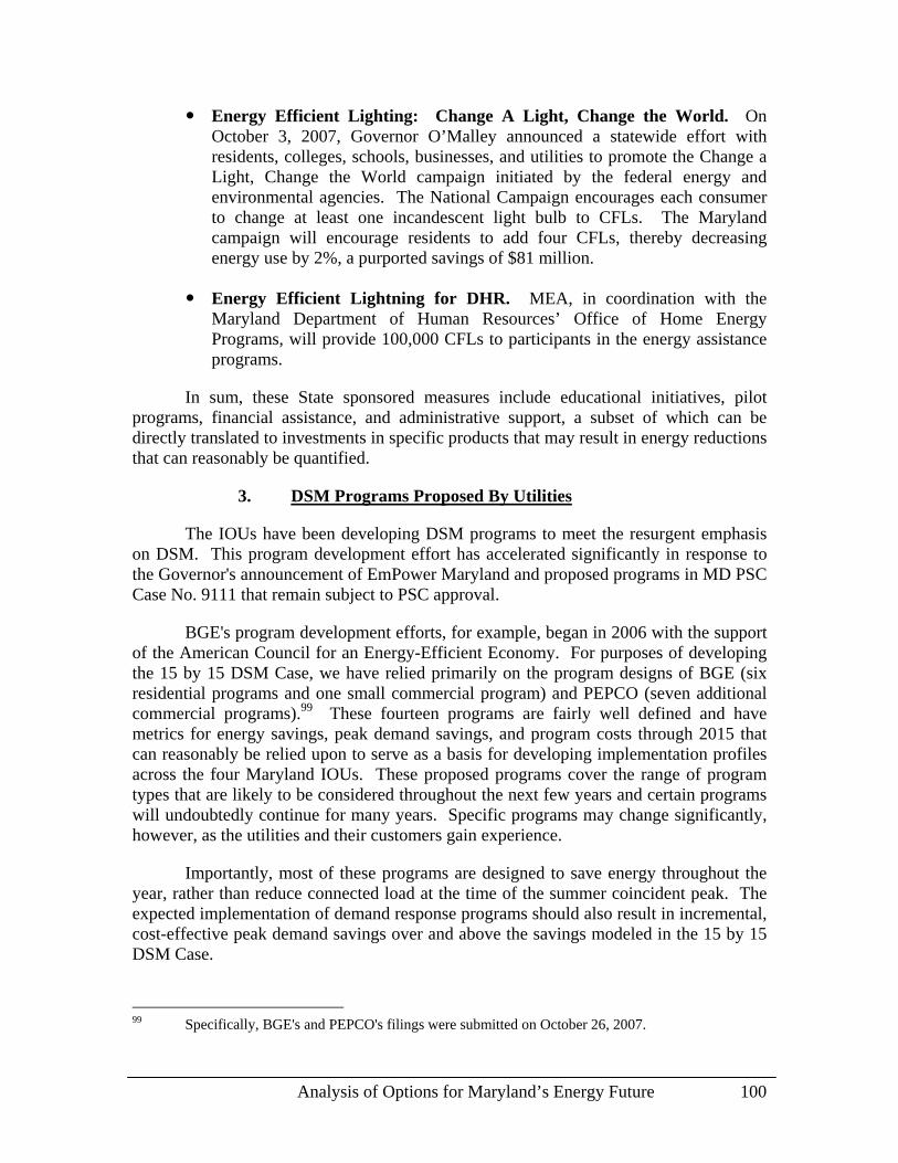
Analysis of Options for Maryland’s Energy Future 100
Energy Efficient Lighting: Change A Light, Change the World. On October 3, 2007, Governor O’Malley announced a statewide effort with residents, colleges, schools, businesses, and utilities to promote the Change a Light, Change the World campaign initiated by the federal energy and environmental agencies. The National Campaign encourages each consumer to change at least one incandescent light bulb to CFLs. The Maryland campaign will encourage residents to add four CFLs, thereby decreasing energy use by 2%, a purported savings of $81 million.
Energy Efficient Lightning for DHR. MEA, in coordination with the
Maryland Department of Human Resources’ Office of Home Energy Programs, will provide 100,000 CFLs to participants in the energy assistance programs.
In sum, these State sponsored measures include educational initiatives, pilot programs, financial assistance, and administrative support, a subset of which can be directly translated to investments in specific products that may result in energy reductions that can reasonably be quantified.
3. DSM Programs Proposed By Utilities
The IOUs have been developing DSM programs to meet the resurgent emphasis on DSM. This program development effort has accelerated significantly in response to the Governor's announcement of EmPower Maryland and proposed programs in MD PSC Case No. 9111 that remain subject to PSC approval.
BGE's program development efforts, for example, began in 2006 with the support of the American Council for an Energy-Efficient Economy. For purposes of developing the 15 by 15 DSM Case, we have relied primarily on the program designs of BGE (six residential programs and one small commercial program) and PEPCO (seven additional commercial programs).99 These fourteen programs are fairly well defined and have metrics for energy savings, peak demand savings, and program costs through 2015 that can reasonably be relied upon to serve as a basis for developing implementation profiles across the four Maryland IOUs. These proposed programs cover the range of program types that are likely to be considered throughout the next few years and certain programs will undoubtedly continue for many years. Specific programs may change significantly, however, as the utilities and their customers gain experience.
Importantly, most of these programs are designed to save energy throughout the year, rather than reduce connected load at the time of the summer coincident peak. The expected implementation of demand response programs should also result in incremental, cost-effective peak demand savings over and above the savings modeled in the 15 by 15 DSM Case.
99 Specifically, BGE's and PEPCO's filings were submitted on October 26, 2007.

Analysis of Options for Maryland’s Energy Future 101
The following summary highlights the programs that were relied upon in developing the 15 by 15 DSM case.
Residential Programs:
ENERGY STAR Lighting (developed by BGE) – targeted rebates to reduce first-cost barriers of lighting products including CFLs;
ENERGY STAR Appliances (BGE) – targeted incentives to purchase energy efficient appliances including dishwashers, clothes dryers, refrigerators, freezers and room air conditioners;
On-Line" Store (BGE) – web-based access to information and incentives to purchase lighting products, water heating blankets, heating system pipe wrap and other efficiency products;
HVAC (BGE) – incentives to promote the purchase and quality installation of efficient heating, cooling, and water heating equipment;
Residential New Construction (BGE) – incentives to builders to build homes that are use at least 15% less energy than required by building codes using the Home Energy Rating System developed by the EPA;
Residential Retrofit (BGE) – free web-based energy audits, subsidized on-site energy audits, and incentives of up to $3,000/home to implement ENERGY STAR-based improvement programs identified during the audits; and
Low Income (BGE) – electric and gas efficiency measures for qualified low-income households that are based on the site-specific characteristics of each home and the application of energy-use diagnostic tools.
Commercial Programs:
Small Commercial Energy Efficiency (BGE) – improvements to lighting and HVAC systems, refrigeration, and small commercial customer end-uses;
Commissioning and O&M (PEPCO) – consulting and engineering services and low-cost/no-cost system adjustments and control system modifications;
Commercial New Construction (PEPCO) – a range of cost-effective energy efficiency measures identified during the design and construction phases for commercial buildings;
HVAC (PEPCO) – incentives for customers to select high efficiency options when making HVAC purchasing decisions;
Prescriptive (PEPCO) – incentives for commercial and industrial customers to select certain high-efficiency options when making purchasing decisions;
Customized Incentive (PEPCO) – incentives for commercial and industrial customers to select high-efficiency options that are customized to the specific needs of the customer; and

Analysis of Options for Maryland’s Energy Future 102
Smart Stat (PEPCO) – installation of remotely controllable thermostats that are capable of reducing air conditioning load upon receipt of a utility command signal.
More detailed descriptions of each of these programs are provided in BGE’s and PEPCO’s October 26, 2007 submittals in MD PSC Case No. 9111.
4. Calculation of Energy and Peak Demand Savings
The 15 by 15 DSM Case is based on Maryland’s four IOUs realizing their proportionate EmPower Maryland energy savings goal of 7,964 GWh by 2015. This is accomplished through a two-step process. First, we have scaled up the BGE and PEPCO programs to statewide IOU program benefits (and costs) as if these programs were applied by all four utilities, including Allegheny and Delmarva. We accomplished this extrapolation by applying PEPCO’s commercial programs only in PEPCO's service territory, applying the BGE residential programs to all four utilities, and applying the BGE’s small commercial programs to APS and Delmarva.100 The relative commitment placed on the set of programs by BGE and PEPCO, respectively, was not altered during this step, i.e., the comparative mix of energy, peak demand savings and program costs.
We did not modify the key design elements for each of the fourteen programs during this first step and include energy and peak demand savings by year, program costs, and hourly load profiles for each of three seasons – winter, summer, and shoulder months. This results in energy savings of 2,514 GWh or 31.6% of the 2015 goal. The associated peak demand savings are 556 MW.101 Utilities incur program costs for administration, marketing, incentives, implementation and evaluation and measurement. Costs incurred by participating customers to pay for equipment and installation that exceed the incentive payments are an additional cost that must be considered when evaluating individual programs.
The second step scales up the four-utility totals to achieve the EmPower Maryland goal for the four IOUs. To accomplish this step, we significantly ramped up the reach of these programs for the residential programs and the small commercial program sufficiently to produce a total savings of 7,964 GWh. In addition, we assumed that the programs would be more costly to implement and would be less effective, reflecting an upward-sloping energy efficiency supply curve. These assumptions and the resulting savings are summarized in Table 13.
100 BGE residential sales represent 54.7 % of total residential sales for all four utilities, and its
commercial sales represent 73.7% of such sales, excluding PEPCO. 101 For purposes of developing the 15 by 15 DSM case, we have made no determination as to the
ability of the recently filed utility programs to meet or exceed their estimated savings objectives.

Analysis of Options for Maryland’s Energy Future 103
Table 13. Upward-Sloping DSM Supply Curve Assumptions
Year
Increase in Reach of
Residential Programs
Increase in Reach of
Commercial Programs
Annual Program
Degradation
Real Cost Escalation
Energy Savings
GWh
Peak Demand Savings
MW 2008 - - 0% 0.0% 228 43 2009 1.25x 2.00x 0% -2.5% 696 132 2010 2.25x 2.75x 0% -0.5% 1,503 311 2011 3.00x 3.50x 0% 3.5% 2,463 520 2012 3.75x 4.25x -4% 7.5% 3,623 771 2013 4.50x 5.00x -6% 11.5% 4,901 1,043 2014 5.25x 5.75x -8% 15.5% 6,387 1,332 2015 6.00x 6.50x -10% 19.5% 7,963 1,642
As shown in Table 13, it is necessary to increase the annual reach of DSM programs by upward of 600% in order to attain the 15 by 15 target. For example, market penetration rates developed by BGE for its small commercial program would have to attract twice as many customers as originally contemplated in the second year of the program (2009) and be subject to increasing multiples for each of the years leading up to 2015. Stated another way, a commercial HVAC program that targeted 2% of customers initially would now target 4% of customers in 2009. As market reach multiples increase, we have assumed that utilities will have to make the programs more attractive to customers that are harder to reach or have lower potential value to be realized by DSM. Thus, we have increased the cost of DSM programs and decreased the energy and peak savings in the latter half of this period. As discussed further below, it should also be noted as well that participants must contribute 50% to 200% of the total costs of installing energy efficient measures, thus creating a further obstacle to increasing penetration rates.
Nevertheless, it is possible that significant portions of the aggressive 15 by 15 target can be met with new programs, reducing the need to rely on increasing penetration rates from the initial programs. Nonetheless, the 15 by 15 targets may prove extremely difficult to reach if resistance proves to be an obstacle for a significant portion of customers.
In order to calculate avoided cost savings using MarketSym, it is necessary to apply load shapes for each program that produce the annual energy and peak demand savings that contribute to the totals reported above. We developed load shapes for each of the fourteen programs for each of three seasons: winter (January, February, and December), summer (June - August) and shoulder (March - May and September - November). We assumed that the peak demand will occur during the hours of 2 to 6 PM on a weekday during a summer month. These load shapes reflect the types of measures delivered by each program.
Figure 47 shows the 2015 aggregated DSM load shape.

Analysis of Options for Maryland’s Energy Future 104
Figure 47. Composite Energy Savings Profile
Peak Reduction, 1,642
0
200
400
600
800
1,000
1,200
1,400
1,600
1,800
1:00
AM
2:00
AM
3:00
AM
4:00
AM
5:00
AM
6:00
AM
7:00
AM
8:00
AM
9:00
AM
10:0
0 A
M
11:0
0 A
M
12:0
0 P
M
1:00
PM
2:00
PM
3:00
PM
4:00
PM
5:00
PM
6:00
PM
7:00
PM
8:00
PM
9:00
PM
10:0
0 P
M
11:0
0 P
M
12:0
0 A
M
Hour Ending
Ener
gy L
oad
Red
uctio
n (M
W)
DEC-FEB JUN-AUG Other
5. Calculation of Program and Participant Costs
BGE’s and PEPCO’s filings estimate costs for each of the fourteen proposed programs. Our cost analysis used the same two-step process that we used to determine energy and peak demand savings. Thus, in the first step, we scaled up costs to a four-utility total by applying the same factors. In the second step, we increased costs proportionately to reflect the increase in market reach levels, and also applied real price increases to reflect an upward sloping DSM supply curve. Table 13 shows these real cost increases above.
The development of participant costs is subject to considerable uncertainty. They were not detailed in the filings of BGE and PEPCO; however, the utilities reported the results of a Participant Test. We developed an estimate of the ratio between participant to program costs for each program based on program descriptions, relative Participant Test results and more detailed participant cost information that APS provided in its October 26, 2007 submittal in MD PSC Case No. 9111.102
Based on this information, we estimated the ratio between participant costs and program costs for each measure. We then applied these ratios or multipliers to the estimate of program costs to derive participant costs.
102 We did not have sufficient detail to perform a “bottoms-up” forecast of participant costs taking
into account the number of installations of energy efficient equipment and the incremental costs of this equipment for replacement of failed equipment.

Analysis of Options for Maryland’s Energy Future 105
Total costs are the sum of these two components. It is also important to note that, unlike program costs, while participant costs increase in proportion to the increase in market penetrations in the DSM Scenario, they were not subject to any nominal cost increase. Thus, we implicitly assumed that the utilities will need to modify programs by increasing the proportion of costs subject to incentives as efficiency increases along the upward sloping DSM supply curve. A summary of the results of the 15 by 15 DSM Case appears in Appendix 6.
As shown in this appendix, based on the assumptions described within this section, total costs to accomplish the 15 by 15 target exceed $4 billion in 2007 dollars. In addition to realizing the energy goal of 7,964 GWh by 2015, the programs create 1,642 MW of peak demand savings at an approximate cost of $2,500/kW. As noted above, additional peak savings will be realized more cost-effectively if Maryland's utilities implement Demand Response programs, as currently contemplated.
IV. Economic Analysis of Selected Options
A. Overview of Analytical Approach
To assess the economic impact of the various potential energy futures for Maryland, we developed with the PSC eight specific Alternative Cases for comparison to a Reference Case. For each case, we defined details regarding the generation fleet, load, and transmission infrastructure and captured those characteristics in energy and capacity market simulation models. We then used these models to produce long-term forecasts of wholesale market prices. We differentiated wholesale energy prices by season and time-of-day over the study period. Our market simulations also provide the dispatched energy output and the energy revenue by generation plant.103 We next transferred the results of the simulation model to a financial model that calculates a cost to serve total customer load in Maryland, including wholesale energy, capacity, and ancillary service costs, direct costs for any generation resource that we assumed would be compensated under a long-term agreement, DSM programs, and transmission costs. We have also quantified the direct benefits of ratepayer backed generation resources or demand side programs. We calculated the cost on an annual basis and on a present value basis over the 20-year study period between 2008 and 2027. Again, the difference in financial value between each Alternative Case and the Reference Case is the EVA.
We used these results to compare the effects of the different resource futures on ratepayers throughout Maryland. Finally, we analyzed the retail rate impact in order to calibrate the effect of different resource options on an average residential customer for each of four IOUs. All EVAs discussed in this section reflect how each resource option compares to the Reference Case, which by definition incorporates our Base Case fuel price forecast. Given the available time and resources, we did not perform any sensitivity analyses to assess other potential changes in external variables, e.g., fuel prices, fuel price
103 For modeling purposes, DSM measures are treated as generation resources, rather than
adjustments to load.

Analysis of Options for Maryland’s Energy Future 106
volatility, gas/oil parity ratios, or environmental regulation. Because these factors could affect the outcomes, we recommend that policy makers undertake extensive sensitivity analyses among leading resource options before finalizing any regulatory incentives to promote new generation or DSM programs.
Although we aggregate the results in the EVA, we identified each cost or benefit component for each case and for each year. Unbundling EVA provides insight into the origin of benefits and costs for different technologies – both supply and demand based. Both benefits and costs can be grouped to provide a more meaningful understanding. – For example, all direct, unavoidable costs associated with an Alternative Case can be grouped in a “Cost” bin, while all other costs and benefits can be netted into a “Benefits” bin. While the net sum of the two bins constitutes EVA, the ratio of the “Benefits” to the “Costs” is one benchmark indicator of the potential at-risk capital, i.e., the amount of capital necessarily tied up under long-term agreements in order to produce net benefits.
It is also useful to differentiate “direct” benefits. This separation distinguishes the market value of the capacity and energy associated with a proposed ratepayer-backed generation option from “indirect” effects, e.g., the change in total load at market energy and capacity prices as well as the change in the value of existing ratepayer-backed programs like the Solar Band or demand response programs.
B. Reference Case Definition
The Reference Case represents Maryland’s long-term energy future in the absence of new initiatives by the Commission, Legislature, or PJM. Holding constant existing transmission topology across the region, the Reference Case is an extension of regional market conditions over the last decade. In formulating the Reference Case, we assumed the following:
PJM’s reliability criteria will be satisfied over the study horizon. There is no unserved load or shortage hours requiring voltage reductions, rotating blackouts, or system-wide outage contingencies.
Simple-cycle GTs added “just in time” will ensure adequate reserve margins
in SWMAAC. These peaker additions will be located in SWMAAC rather than the District of Columbia. To keep supply and demand in balance, merchant GTs will be added over the forecast period in 220 MW increments. Reserve margins in the APS and EMAAC areas will be met primarily by a mixture of types of additions outside of Maryland.104 GTs will be attributed to Maryland to the extent they are needed for local reliability. The new units will be merchant generators rather than utility-backed under either PPAs or tolling agreements and will reflect merchant investment risk in their capital
104 Except for one coal plant – assumed to be in service in 2012 in the West Virginia portion of APS –
we assume that PJM resource additions will be predominantly GTs, also under merchant entry assumptions.
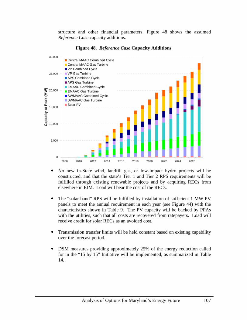
Analysis of Options for Maryland’s Energy Future 107
structure and other financial parameters. Figure 48 shows the assumed Reference Case capacity additions.
Figure 48. Reference Case Capacity Additions
0
5,000
10,000
15,000
20,000
25,000
30,000
2008 2010 2012 2014 2016 2018 2020 2022 2024 2026
Cap
acity
at P
eak
(MW
)
Central MAAC Combined CycleCentral MAAC Gas TurbineVP Combined CycleVP Gas TurbineAPS Combined CycleAPS Gas TurbineEMAAC Combined CycleEMAAC Gas TurbineSWMAAC Combined CycleSWMAAC Gas TurbineSolar PV
No new in-State wind, landfill gas, or low-impact hydro projects will be constructed, and that the state’s Tier 1 and Tier 2 RPS requirements will be fulfilled through existing renewable projects and by acquiring RECs from elsewhere in PJM. Load will bear the cost of the RECs.
The “solar band” RPS will be fulfilled by installation of sufficient 1 MW PV
panels to meet the annual requirement in each year (see Figure 44) with the characteristics shown in Table 9. The PV capacity will be backed by PPAs with the utilities, such that all costs are recovered from ratepayers. Load will receive credit for solar RECs as an avoided cost.
Transmission transfer limits will be held constant based on existing capability
over the forecast period.
DSM measures providing approximately 25% of the energy reduction called for in the “15 by 15” Initiative will be implemented, as summarized in Table 14.

Analysis of Options for Maryland’s Energy Future 108
Table 14. Reference Case DSM Assumptions
Year Energy Reduction GWh Peak Load Reduction, MW Program and Participant
Cost, 2007 $MM Residential Commercial Residential Commercial Residential Commercial2008 176.8 81.4 26.4 10.3 $69.8 $33.0 2009 355.0 163.4 53.1 20.7 $68.1 $32.4 2010 534.6 246.2 79.9 31.2 $96.2 $40.1 2011 713.8 331.4 107.0 42.0 $84.4 $38.3 2012 894.4 417.4 134.3 52.9 $75.3 $37.6 2013 1,074.7 505.9 161.8 64.1 $59.7 $35.6 2014 1,256.4 595.1 189.5 75.4 $46.4 $29.6 2015 1,439.9 685.1 217.5 86.8 $37.1 $28.8 2016 1,525.6 725.9 230.5 92.0 $28.3 $9.9 2017 1,612.9 767.4 243.7 97.2 $29.8 $10.5 2018 1,701.7 809.6 257.1 102.6 $31.4 $11.0 2019 1,791.8 852.5 270.7 108.0 $33.1 $11.6 2020 1,883.5 896.1 284.5 113.6 $34.9 $12.2 2021 1,976.6 940.4 298.6 119.2 $36.8 $12.9 2022 2,071.2 985.5 312.9 124.9 $38.7 $13.6 2023 2,071.2 985.5 312.9 124.9 $0.0 $0.0 2024 2,071.2 985.5 312.9 124.9 $0.0 $0.0 2025 2,071.2 985.5 312.9 124.9 $0.0 $0.0 2026 2,071.2 985.5 312.9 124.9 $0.0 $0.0 2027 2,071.2 985.5 312.9 124.9 $0.0 $0.0
1. Modeling Results
(a) Wholesale Energy Prices
The MarketSym simulation model run for the Reference Case provides a baseline set of hourly wholesale LMPs in the relevant zones. Figure 49 summarizes the average annual prices in each year of the study period for APS, EMAAC (Delmarva), and SWMAAC (BGE and PEPCO).

Analysis of Options for Maryland’s Energy Future 109
Figure 49. Reference Case Energy Prices
40
60
80
100
120
140
160
2008 2010 2012 2014 2016 2018 2020 2022 2024 2026
Tim
e-W
td A
vg P
rice
($/M
Wh)
APSEMAACSWMAAC
The wholesale energy prices that load pays largely determine the overall impact of changes in generation capacity and other measures considered in this study. We developed load profiles were developed for each of the IOUs covering eligible customers under Residential and Types I, II, and III rate classes. We matched the hourly load profiles – increased at 1% per year from the base data for 2006 – against the hourly energy price forecasts from the MarketSym simulations to develop the MTM wholesale cost of load. Figure 50 shows the total annual costs for each utility under the Reference Case assumptions.

Analysis of Options for Maryland’s Energy Future 110
Figure 50. Reference Case Load at Market Energy Price
0
2,000
4,000
6,000
8,000
10,000
12,000
2008 2010 2012 2014 2016 2018 2020 2022 2024 2026
Ann
ual L
oad
MTM
($ M
illio
ns)
Allegheny BG&E Delmarva Pepco
(b) Capacity Prices
Figure 51 summarizes the resulting capacity prices for the Reference Case using our modeling technique to project UCAP prices consistent with PJM’s RPM auctions. After 2008, prices for the four utilities are essentially identical through 2014, when transmission limitations cause prices in the SWMAAC LDA (BGE and PEPCO service territories) to rise above those of the MAAC LDA (APS and Delmarva service territories).

Analysis of Options for Maryland’s Energy Future 111
Figure 51. UCAP Price Forecast – Reference Case
0
50
100
150
200
250
300
350
2008 2010 2012 2014 2016 2018 2020 2022 2024 2026
UC
AP
Pric
e ($
/MW
-day
)Allegheny Delmarva BG&E / Pepco
(c) Generation Service Costs
Our financial model for this study uses the energy load MTM, case-specific forecast of UCAP prices, and incorporates the value of ancillary services to develop a total cost for generation and transmission services. The wholesale power cost represented in the model also includes PJM transmission costs, the net effects of any PPA arrangements for solar or other generation, and the net effects of DSM initiatives. Figure 43 summarizes the total annual costs for the Reference Case. The bars for the energy and capacity benefits of solar and DSM initiatives are below the x-axis, representing credits against total cost.105
105 We did not attempt to distinguish between direct participant costs and benefits, and socialized
costs and benefits for the DSM initiatives. Similarly, we treated all costs and benefits of the Solar Band initiative as if they were socialized among all eligible ratepayers.

Analysis of Options for Maryland’s Energy Future 112
Figure 52. Reference Case Annual Costs
(2,000)
0
2,000
4,000
6,000
8,000
10,000
12,000
14,000
16,000
2008
2010
2012
2014
2016
2018
2020
2022
2024
2026
Ann
ual C
ost (
$ M
illio
ns)
Solar EnergyMarket ValueSolar CapacityMarket ValueDSM ProgramCapacity SavingsDSM ProgramEnergy SavingsSolar ProgramDirect CostsDSM ProgramDirect CostsPJM TransmissionCostsUnadjusted MarketCapacity CostUnadjusted MarketEnergy CostTotal Cost
The present value of this string of annual costs for the Reference Case of $72.96 billion establishes the baseline for determining EVA. Of critical importance, we use this total cost to serve wholesale load in Maryland as a reasonable benchmark for analyzing the difference in total costs under rival technology options examined. Because other variables or new PJM rules or environmental regulations could affect market prices, the actual costs to serve wholesale load over the planning horizon may differ materially from these long-term projections.
C. Alternative Case Definitions
1. Optimum Mix Case
In this case, we assume that new generation installed in Maryland to meet reserve margin requirements consists of the optimal mix of gas-fired GT and CC capacity rather than only GTs. Instead of a 220 MW GT addition in 2012 in SWMAAC, we tested the addition of a single 230 MW combined cycle plant to meet reliability criteria. The annual capacity factors of this unit ranged between 40% and 50%. We assumed that all new capacity would be merchant-owned and would participate in the wholesale capacity and energy markets based on UCAP prices under RPM and energy margins associated with the spread between LMPs and the marginal cost of producing energy based on the TZ6NNY mid-point gas price, adjusted for non-fuel variable O&M expense. . Resource additions elsewhere in PJM, transmission infrastructure, and load assumptions are the same as the Reference Case.

Analysis of Options for Maryland’s Energy Future 113
(a) Resource Additions
The “optimized” merchant capacity mix for this case resulted in the installation of a single CC unit in 2011, offset by the elimination of a GT unit from the capacity mix delineated in the Reference Case in 2012. Both of these changes occur in SWMAAC. Resource additions outside Maryland are the same as Reference Case.
(b) Wholesale Energy Prices
The Optimum Mix Case has a small, but significant effect on wholesale energy prices. This price reduction continues in SWMAAC over the study period, however. The energy price effect in adjoining areas is negligible.
(c) Capacity Prices
The Optimum Mix Case has a negligible and brief effect on capacity prices in 2011, the only year with a significant beneficial effect attributable to the temporary generation surplus. Figure 45 magnifies the impact because the scale of the y-axis is very large. The MW surplus is soon depleted as a result of the avoided GT unit in 2012.
(d) Generation Service Costs
The introduction of a merchant combined cycle unit in SWMAAC has the effect of reducing market energy prices in most future years, thus providing benefits throughout most of Maryland. The beneficial capacity price impact is short term only, however. As Figure 53 shows, project EVA is $196 million. Because we have treated the introduction of the combined cycle plant under merchant entry conditions, there are no identifiable direct costs allocable to ratepayers. Therefore, the benefit-to-cost ratio is meaningless.

Analysis of Options for Maryland’s Energy Future 114
Figure 53. Annual Cost Savings – Optimum Mix Case
(60)
(40)
(20)
0
20
40
60
80
100
2008
2010
2012
2014
2016
2018
2020
2022
2024
2026
Ann
ual C
ost S
avin
gs v
. Ref
eren
ce ($
Mill
ions
)Solar EnergyMarket Value
Solar CapacityMarket Value
DSM ProgramCapacity Savings
DSM ProgramEnergy Savings
Unadjusted MarketCapacity Cost
Unadjusted MarketEnergy Cost
Total Savings
2. Coal Case
In this case, we have postulated that utilities in Maryland would enter into a long-term contract with a developer to build and operate a 648 MW supercritical pulverized coal unit with state-of-the-art pollution control systems in SWMAAC. The assumed in-service date is 2015. In response to a regulatory directive from the PSC or other Legislative initiative, the PPA would provide for a fixed capacity payment designed to allow the developer to achieve full recovery of capital and a reasonable return on capital over the contract term.106 We have assumed an inflation-indexed fixed O&M payment, and a call option on energy production at a price based on the cost of coal plus an inflation-indexed variable O&M charge. In other words, ratepayers would assume responsibility for all reasonably incurred costs associated with building and operating the coal plant.
(a) Resource Additions
The addition of a 648 MW baseload coal unit in 2015 permits Maryland to avoid about 650 MW of gas turbine capacity additions that would otherwise be required to maintain reliability. The addition of this baseload coal plant would also trigger other
106 As we discussed elsewhere in this Interim Report, a PPA may not be the preferred contractual
structure for long-term power procurement. A financial arrangement in the form of a CfD may have significant advantages.

Analysis of Options for Maryland’s Energy Future 115
capacity deferrals outside SWMAAC, but the price impact would be insignificant. Figure 54 summarizes the addition of the coal unit and solar band.
Figure 54. Ratepayer-Backed Capacity – Coal Case
0
200
400
600
800
1,000
1,200
2008 2010 2012 2014 2016 2018 2020 2022 2024 2026
Rat
epay
er-B
acke
d C
apac
ity (M
W)
Solar PVWindNuclearCoalCombined CycleSimple Cycle Gas Turbine
(b) Wholesale Energy Prices
The Coal Case would significantly reduce energy prices in SWMAAC from its commercial operation date through the remainder of the study horizon. Absent other transmission upgrades, however, the price effect in adjacent sub-areas would be negligible.
Figure 55 shows the price impact on annual average energy prices on a time-weighted basis.

Analysis of Options for Maryland’s Energy Future 116
Figure 55. Wholesale Energy Prices -- Coal Case
40
60
80
100
120
140
160
2008 2010 2012 2014 2016 2018 2020 2022 2024 2026
Tim
e-W
td A
vg P
rice
($/M
Wh)
APS APS (Reference Case)EMAAC EMAAC (Reference Case)SWMAAC SWMAAC (Reference Case)
(c) Capacity Prices
Because the baseload resource creates a short-term generation surplus, the Coal Case produces a relatively small and transient beneficial impact on UCAP prices over a three-year period following commercial start-up. Figure 56 shows that the capacity surplus will permit the cancellation or deferral of gas turbine units that would otherwise be necessary, and the system will again return to equilibrium causing capacity prices to rebound.

Analysis of Options for Maryland’s Energy Future 117
Figure 56. Differential Capacity Prices – Coal Case
(16)
(14)
(12)
(10)
(8)
(6)
(4)
(2)
0
2
2008 2010 2012 2014 2016 2018 2020 2022 2024 2026
Cha
nge
in U
CA
P Pr
ice
($/M
W-d
ay)
Allegheny Delmarva BG&E / Pepco
(d) Generation Service Costs
Although the beneficial effect on capacity costs is limited to three years, a new coal unit in SWMAAC reduces energy prices in all years following commercial start-up. As Figure 57 shows, other effects include the direct costs of the coal unit and the associated net energy margin and capacity value. Project EVA is $888 million. The present value of the benefits relative to the present value of the direct PPA costs produces a benefit-to-cost ratio of 1.68.107
107 Given this benefit-to-cost ratio, there may be sufficient price incentive based on energy and
capacity prices for a developer to merchandise a coal generation plant in SWMAAC, thereby transferring the market and operational risk from the utilities’ load to the supplier. We were not asked to analyze how such increased risk would be priced into the transaction.

Analysis of Options for Maryland’s Energy Future 118
Figure 57. Annual Cost Savings – Coal Case
(400)
(200)
0
200
400
600
800
2008
2010
2012
2014
2016
2018
2020
2022
2024
2026
Ann
ual C
ost S
avin
gs v
. Ref
eren
ce ($
Mill
ions
)Coal CapacityValue
Coal Net EnergyMargin
Coal Direct Costs
Solar EnergyMarket Value
Solar CapacityMarket Value
DSM ProgramCapacity Savings
DSM ProgramEnergy Savings
Unadjusted MarketCapacity Cost
Unadjusted MarketEnergy Cost
Total Savings
3. Nuclear Case
High energy prices, coupled with global concerns about greenhouse gas emissions, have stimulated renewed interest in nuclear power after a nearly three-decade hiatus in new nuclear construction in the U.S. In the Nuclear Case, we assume the addition of a new 1600 MW unit at the Calvert Cliffs station owned and operated by Constellation with an in-service date of 2017. To ensure bulk power reliability, we continued to assume that gas turbines will be added from 2008 through 2016, as in the Reference Case. The additional nuclear plant in 2017 will create a large capacity surplus in SWMAAC. Once load growth and retirements deplete that capacity surplus, we again assume that new entry will be limited to gas turbines.
Constellation is seriously considering a new nuclear unit at Calvert Cliffs, where there is apparently available space, community acceptance, and adequate transmission interconnections. Investment in new nuclear stations is a federal priority, thereby making available potential debt guarantees and financial incentives. Constellation has a strong balance sheet, a strong nuclear operating record, and a partnership with a major French reactor vendor.108 Global concerns about greenhouse gas emissions, coupled with increased federal incentives, make the nuclear option a reasonable complement to the 108 We have not evaluated whether price signals alone are sufficient to allow Constellation to add a
third nuclear power plant on a merchant basis. For the Nuclear Case, we made the simplifying assumption that the PSC directs Maryland’s IOUs to enter into long-term agreements to purchase all of the generation output from a new nuclear unit.

Analysis of Options for Maryland’s Energy Future 119
array of rival supply and demand based technologies that we examined in this study. If the PSC were to direct Maryland’s utilities to enter long-term contracts to facilitate the addition of a new nuclear plant, we have assumed that the majority of the capital cost, timing and long term performance risks would be borne by the supplier. Although the operating risk would remain with the supplier, we have made the assumption that the IOUs’ ratepayers would bear market price risks, regulatory risks, and financial risks.
(a) Resource Additions
Given the long lead time for NRC approval and construction, we assume commercial start-up in 2017. Only then would the nuclear plant permit deferral of other capacity alternatives in SWMAAC and surrounding areas. Addition of new nuclear capacity at Calvert Cliffs would cancel or defer about 1,600 MW of gas turbine capacity in Maryland. In Figure 58 we summarize the amount of new capacity in the Nuclear Case under long term PPAs.
Figure 58. Ratepayer-Backed Capacity – Nuclear Case
0
500
1,000
1,500
2,000
2,500
2008 2010 2012 2014 2016 2018 2020 2022 2024 2026
Rat
epay
er-B
acke
d C
apac
ity (M
W)
Solar PVWindNuclearCoalCombined CycleSimple Cycle Gas Turbine
(b) Wholesale Energy Prices
The Nuclear Case has a substantial favorable impact on energy prices in SWMAAC from 2017 through the remainder of the study horizon. Due to continued transmission constraints between SWMAAC and the Delmarva Peninsula, however, the impacts of a third nuclear power plant on energy prices in EMAAC and APS will be insignificant. Figure 59 shows the impacts on annual average energy prices

Analysis of Options for Maryland’s Energy Future 120
Figure 59. Nuclear Case Energy Prices
40
60
80
100
120
140
160
2008 2010 2012 2014 2016 2018 2020 2022 2024 2026
Tim
e-W
td A
vg P
rice
($/M
Wh)
APS APS (Reference Case)EMAAC EMAAC (Reference Case)SWMAAC SWMAAC (Reference Case)
(c) Capacity Prices
After 2017, the Nuclear Case sustains significant downward pressure on UCAP prices in SWMAAC for nearly all of the remaining study horizon until load growth depletes the generation surplus. The reduction in UCAP prices would be especially beneficial for BGE and PEPCO customers. As with energy prices, transmission constraints make the UCAP price effects in EMAAC and APS relatively insignificant. Figure 60 shows the projected differential on capacity prices relative to the Reference Case.

Analysis of Options for Maryland’s Energy Future 121
Figure 60. Differential Capacity Prices – Nuclear Case
(35)
(30)
(25)
(20)
(15)
(10)
(5)
0
5
2008 2010 2012 2014 2016 2018 2020 2022 2024 2026
Cha
nge
in U
CA
P Pr
ice
($/M
W-d
ay)
Allegheny Delmarva BG&E / Pepco
(d) Generation Service Costs
The addition of a third nuclear unit depresses UCAP prices and energy prices in SWMAAC, producing robust economic benefits for ratepayers. Given the high capital-intensiveness of nuclear power as well as the study paradigm, namely, the transference of market, financial, and regulatory risk to load, ratepayers would bear high capacity charges irrespective of the market value of UCAP under the RPM. As shown in Figure 61 the annual cost savings from 2017 through the end of the study horizon are large each and every year following commercial start-up of a third nuclear power plant in Maryland. The project EVA for the Nuclear Case is $2.9 billion. The benefit-to-cost ratio is 2.05.109 Importantly, the majority of the net benefits associated with the new nuclear unit are energy related – by far the most unstable and volatile component of total benefits in light of the inherent volatility in oil and gas markets over the study horizon. Thus, the Nuclear Case provides both a physical and financial hedge against the fundamental uncertainty associated with premium fossil fuel prices over the long term. To the extent oil and natural gas prices are higher than those used in the Base Case fuel price forecast
109 It is possible that energy and UCAP price signals coupled with advantageous loan guarantees from
the federal government, may be sufficient to induce nuclear entry on a merchant basis, but that question is the outside the scope of our assigned analysis.

Analysis of Options for Maryland’s Energy Future 122
incorporated in the Reference Case, project EVA would be higher than $2.9 billion, and vice versa.110
Figure 61. Annual Cost Savings – Nuclear Case
(1,500)
(1,000)
(500)
0
500
1,000
1,500
2,000
2,500
2008
2010
2012
2014
2016
2018
2020
2022
2024
2026
Ann
ual C
ost S
avin
gs v
. Ref
eren
ce ($
Mill
ions
)
Nuclear CapacityValue
Nuclear Net EnergyMargin
Nuclear DirectCosts
Solar EnergyMarket Value
Solar CapacityMarket Value
DSM ProgramCapacity Savings
DSM ProgramEnergy Savings
Unadjusted MarketCapacity Cost
Unadjusted MarketEnergy Cost
Total Savings
4. 15 by 15 DSM Case
Under the 15 by 15 DSM Case, we assume that Maryland will deploy incentives that aggressively implement the Governor’s EMPower Initiative. A portion of this program initiative – about 25% – is embedded in the Reference Case, but we capture the remaining conservation objective in the 15 by 15 DSM Case. We have assumed that fully achieving the 15 by 15 objective will reduce energy use throughout Maryland by 8,500 GWh by 2015. For purposes of calculating rate impacts, we attribute 94% share of statewide energy savings to the four largest IOUs – i.e., 7,964 GWh by 2015. This energy use reduction is measured as the differential between the projected energy use in 2015 with and without implementing the array of conservation programs associated with the “15 by 15” Initiative. We have assumed that DSM efforts would continue to grow at the same rate as the increase in customers, 1% per year. Thus, after 2015 we have projected a continuation of the per capita energy use reductions through 2022. After 2022 we assume no incremental reductions.
Section IV describes the energy efficiency measures that we assume will be used to achieve the target saturation rate.111 Relative to the Reference Case, the incremental 110 Determination of capital at-risk associated with a new nuclear power plant under long term PPAs
is outside the scope of this inquiry.

Analysis of Options for Maryland’s Energy Future 123
energy usage reduction, incremental peak load reduction, and incremental program capital costs dictate the EVA. Table 15 summarizes the aggregated inputs for residential and commercial measures.
Table 15. 15 by 15 DSM Case Incremental Effects
Year Energy Reduction, GWh Peak Load Reduction, MW
Program and Participant Cost, 2007 $MM
Residential Commercial Residential Commercial Residential Commercial 2008 (22.0) (8.4) 4.7 1.1 $0.0 $0.0 2009 148.2 29.6 48.1 9.9 $85.1 $33.0 2010 575.1 147.5 144.5 55.8 $218.8 $53.5 2011 1,142.4 275.4 269.1 101.8 $299.6 $70.1 2012 1,835.2 475.6 421.8 161.6 $389.4 $89.0 2013 2,645.3 675.6 598.3 219.0 $473.1 $106.1 2014 3,576.8 958.6 801.2 265.8 $574.7 $126.9 2015 4,613.0 1,225.4 1,025.8 311.7 $651.5 $142.3
The acceleration in program implementation efforts relative to the Reference Case occurs over the 2009-2015 period. Energy effects are held relatively constant for the period 2016-2027 and no significant new program or participant costs are incurred. The 15 by 15 DSM Case reflects a modest delay in the implementation of new programs based on the recently filed updates to utility DSM plans in Case No. 9111.
(a) Resource Additions
In addition to avoided energy use, the DSM measures allow the incremental deferral or cancellation of up to 1,322 MW of new generation capacity that would otherwise be required. Figure 62 shows capacity differentials relative to the Reference Case.
111 Incorporation of the target saturation rate requires adjustments to load profiles in MarketSym. We
apportioned 70% of the load reduction in SWMAAC and divided the remainder evenly between EMAAC and APS.

Analysis of Options for Maryland’s Energy Future 124
Figure 62. 15 by 15 DSM Case Capacity Changes
(1,600)
(1,400)
(1,200)
(1,000)
(800)
(600)
(400)
(200)
0
200
2008 2010 2012 2014 2016 2018 2020 2022 2024 2026
Cap
acity
at P
eak
(MW
)
Central MAAC CombinedCycleCentral MAAC Gas Turbine
VP Gas Turbine
APS Gas Turbine
EMAAC Gas Turbine
SWMAAC Gas Turbine
(b) Wholesale Energy Prices
The 15 by 15 DSM Case significantly reduces wholesale energy prices in SWMAAC over the entire study period. Given the assumed allocation of program benefits in Maryland, the price impacts in APS and EMAAC are not significant. Figure 63 depicts the beneficial price effect on annual average prices on a time-weighted basis.

Analysis of Options for Maryland’s Energy Future 125
Figure 63. 15 by 15 DSM Case Energy Prices
40
60
80
100
120
140
160
2008 2010 2012 2014 2016 2018 2020 2022 2024 2026
Tim
e-W
td A
vg P
rice
($/M
Wh)
APS APS (Reference Case)EMAAC EMAAC (Reference Case)SWMAAC SWMAAC (Reference Case)
As this figure shows, the impacts in SWMAAC are larger because the leftward shift in the demand curve created by aggressive DSM policies occurs primarily in this region.
(c) Capacity Prices
Because the 15 by 15 DSM Case is based on reductions in per capita usage rather than reductions in peak usage, it has a relatively small impact on UCAP prices in SWMAAC. A different DSM program design focused on reducing peak demand could produce greater capacity price reductions, but we have not studied these alternatives. Figure 64 shows forecasted differential capacity prices. Again, most of the reduction occurs in the SWMAAC, thereby benefiting ratepayers served by BGE and PEPCO.

Analysis of Options for Maryland’s Energy Future 126
Figure 64. Differential Capacity Prices – 15 by 15 DSM Case
(12)
(10)
(8)
(6)
(4)
(2)
0
2
2008 2010 2012 2014 2016 2018 2020 2022 2024 2026
Cha
nge
in U
CA
P Pr
ice
($/M
W-d
ay)
Allegheny Delmarva BG&E / Pepco
(d) Generation Service Costs
Successful conservation incentives significantly reduce energy prices, thereby providing ratepayers with material economic and environmental benefits, but the modeled programs do not change UCAP clearing prices significantly. As Figure 65 shows, the net energy and capacity savings substantially offset the direct costs of conservation measures, yielding economic benefits each and every year over the study horizon. As the target saturation rate for DSM is achieved over time, the economic benefits steadily increase. The EVA for the 15 by 15 Case is $2.3 billion. The benefit-to-cost ratio is 1.77.
These economic results of the 15 by 15 DSM Case are encouraging. We note, however, that they are predicated on what appear to be extremely aggressive market penetration rates throughout Maryland. Because no other state has achieved such aggressive market penetration rates, there is no hard evidence that they are feasible.112 Moreover, there is considerable uncertainty about the incremental costs associated with energy efficiency programs in order to achieve the aggressive saturation rate underlying the “15 by 15” Initiative.
112 We did not attempt to monetize any loss of consumer preference resulting from the reduction in
energy use or the “quality” of energy used.

Analysis of Options for Maryland’s Energy Future 127
Figure 65. Annual Cost Savings – 15 by 15 DSM Case
(600)
(400)
(200)
0
200
400
600
800
1,000
1,200
1,400
2008
2010
2012
2014
2016
2018
2020
2022
2024
2026
Ann
ual C
ost S
avin
gs v
. Ref
eren
ce ($
Mill
ions
)Solar CapacityMarket Value
Solar EnergyMarket Value
DSM ProgramCapacity Savings
DSM ProgramEnergy Savings
DSM ProgramDirect Costs
Unadjusted MarketCapacity Cost
Unadjusted MarketEnergy Cost
Total Savings
DSM costs include both program costs (incurred either by the utility or any other third-party sponsor) and costs incurred by participants. The annual costs provide a stream of benefits over several years. Thus, we annuitized that stream of benefits to make the comparison with annual savings more relevant.
5. Transmission Case
The addition of backbone transmission into Maryland will change the fundamental market dynamics in SWMAAC. For this case, we postulate that the 502 Junction to Loudoun transmission project approved by PJM is placed in service by 2015. Based on information from PJM, the transfer limits into MAAC by 5000 MW and by 4000 MW into SWMAAC.113 Other transmission highway projects that may inherently compete with the 502 Junction to Loudoun transmission project would also benefit Maryland, but have not been evaluated in this study.114 One of four transmission highway projects endorsed by PJM – the 502 Junction to Loudoun transmission project –
113 We have not conducted any transmission load flow and stability analyses in order to compute the
change in transfer limits into Maryland. 114 We have not conducted any independent transmission load flow or economic analysis of the
comparative benefits of the Amos-Kemptown/Allegheny Mountain project, the Susquehanna-Roseland 500 kV line, or the Possum Point-Calvert Cliffs 500 kV line in this study. Our selection of the 502 Junction to Loudoun project, therefore, is a “placeholder” assumption about the value of high voltage transmission in Maryland and should not be misconstrued as an endorsement of one transmission enhancement over another.

Analysis of Options for Maryland’s Energy Future 128
would surely confer both economic and reliability benefits into both MAAC and SWMAAC. As we discussed previously, this project is estimated to cost $906 million in 2007 dollars. Under FERC approved ratemaking criteria, roughly 10.5% of this expenditure would be allocable to ratepayers in Maryland based on each utility’s contribution to PJM’s total coincident peak.115 Thus, annual incremental PJM transmission charges in Maryland would be approximately $23 million per year, a relatively small increase in total wholesale energy costs. The remaining annual fixed costs – which we estimate at $175 to $196 million –would be socialized across PJM.
Our assumed in-service date associated with the 502 Junction-Loudoun project is uncertain. As of November 2007, none of the PJM Board approved highway projects has been permitted. Despite streamlined permitting procedures enacted by Congress under EPAct 05, many complex siting challenges across multiple state jurisdictions remain that may take years to resolve. Commission action to stimulate new entry or reduce the demand for electricity in Maryland may have a direct bearing on both the economic and reliability rationale underlying the 502 Junction-Loudoun project or the other proposed projects.
(a) Resource Additions
The addition of the 502 Junction-Loudoun line would permit the cancellation of gas turbine capacity that would otherwise be necessary to meet reliability standards in SWMAAC and, to a lesser extent, in EMAAC. Figure 66 shows capacity differentials relative to the Reference Case.
115 Opinion No. 494.

Analysis of Options for Maryland’s Energy Future 129
Figure 66. Transmission Case Capacity Changes
(3,000)
(2,000)
(1,000)
0
1,000
2,000
3,000
2008 2010 2012 2014 2016 2018 2020 2022 2024 2026
Cap
acity
at P
eak
(MW
)
Central MAAC Gas Turbine
VP Gas Turbine
APS Gas Turbine
SWMAAC Gas Turbine
(b) Wholesale Energy Prices
The Transmission Case sustains very significant downward pressure on wholesale energy prices in the SWMAAC over the remaining term of the study horizon.116 Price effects in adjacent sub-areas are much less pronounced, but because the new transmission line will tend to equalize prices across PJM zones, there will be a small wholesale price increase in APS. Figure 67 shows the impact on annual average energy prices on a time-weighted basis.
116 According to PJM’s analysis for base year 2013 both with and without the 502 Junction Loudoun
line, for that year, BGE and PEPCO will realize even greater price benefits.
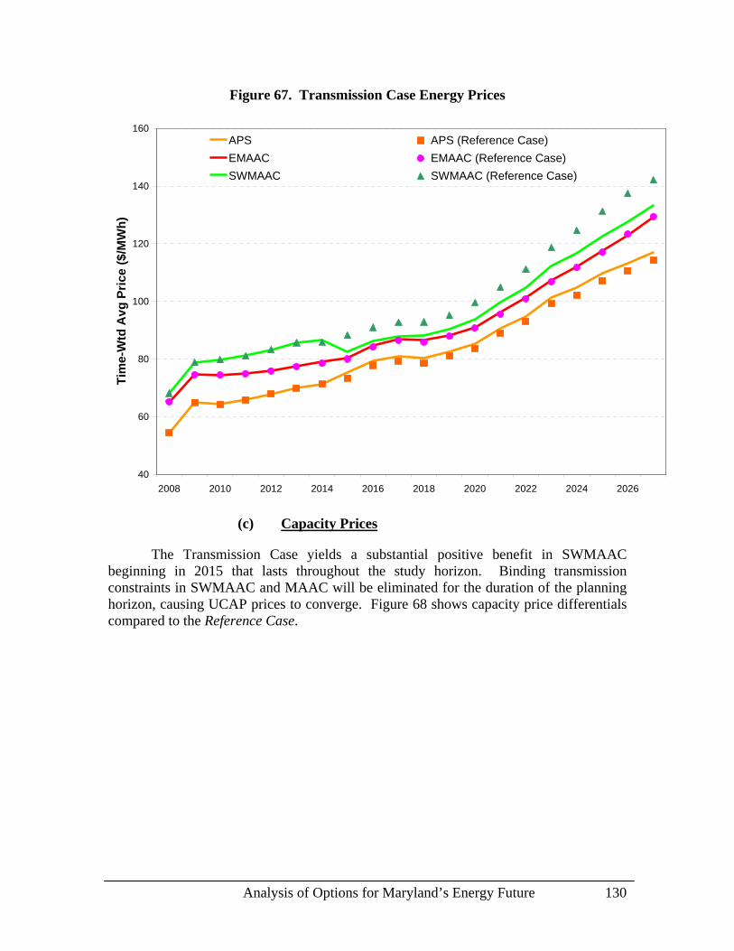
Analysis of Options for Maryland’s Energy Future 130
Figure 67. Transmission Case Energy Prices
40
60
80
100
120
140
160
2008 2010 2012 2014 2016 2018 2020 2022 2024 2026
Tim
e-W
td A
vg P
rice
($/M
Wh)
APS APS (Reference Case)EMAAC EMAAC (Reference Case)SWMAAC SWMAAC (Reference Case)
(c) Capacity Prices
The Transmission Case yields a substantial positive benefit in SWMAAC beginning in 2015 that lasts throughout the study horizon. Binding transmission constraints in SWMAAC and MAAC will be eliminated for the duration of the planning horizon, causing UCAP prices to converge. Figure 68 shows capacity price differentials compared to the Reference Case.

Analysis of Options for Maryland’s Energy Future 131
Figure 68. Differential Capacity Prices – Transmission Case
(70)
(60)
(50)
(40)
(30)
(20)
(10)
0
10
2008 2010 2012 2014 2016 2018 2020 2022 2024 2026
Cha
nge
in U
CA
P Pr
ice
($/M
W-d
ay)
Allegheny Delmarva BG&E / Pepco
(d) Generation Service Costs
The large increase in transmission capacity into SWMAAC reduces market energy prices and capacity prices from 2015 through the end of the study horizon, with benefits flowing primarily to BGE and PEPCO. As Figure 69 shows, only a small portion of the cost of constructing the transmission project would be allocable to Maryland’s ratepayers. The economic benefits would be large throughout the remainder of the study horizon. The EVA for the Transmission Case is $2.2 billion. The benefit-to-cost ratio of 21.4 is extremely high.

Analysis of Options for Maryland’s Energy Future 132
Figure 69. Annual Cost Savings – Transmission Case
(200)
(100)
0
100
200
300
400
500
600
700
800
2008
2010
2012
2014
2016
2018
2020
2022
2024
2026
Ann
ual C
ost S
avin
gs v
. Ref
eren
ce ($
Mill
ions
) Solar CapacityMarket Value
Solar EnergyMarket Value
DSM ProgramCapacity Savings
DSM ProgramEnergy Savings
PJM TransmissionCosts
Unadjusted MarketCapacity Cost
Unadjusted MarketEnergy Cost
Total Savings
6. Wind Case
In the Wind Case, we assumed that 500 MW of state-of-the-art turbines will be installed in Maryland by 2012. To ensure wind entry both onshore and offshore, we assumed that the Commission would encourage Maryland’s utilities to enter in long-term contracts. The total installed capability of the wind units is 500 MW – 200 MW in Western Maryland and 300 MW off the coast of Maryland’s Eastern Shore.
(a) Resource Additions
The wind generation capacity additions occur from 2008 through 2012. The onshore UCAP value of the wind plant is only 28 MW, producing no changes to the APS zone resource additions. The offshore UCAP value is 75 MW, resulting in the deferral of up to 100 MW of gas turbine units in EMAAC.

Analysis of Options for Maryland’s Energy Future 133
Figure 70. Ratepayer-Backed Capacity – Wind Case
0
100
200
300
400
500
600
2008 2010 2012 2014 2016 2018 2020 2022 2024 2026
Rat
epay
er-B
acke
d C
apac
ity (M
W)
Solar PVWindNuclearCoalCombined CycleSimple Cycle Gas Turbine
(b) Wholesale Energy Prices
The Wind Case has an insignificant effect on wholesale energy prices in SWMAAC, but they would produce a minor reduction in EMAAC.
(c) Capacity Prices
The addition of wind turbines would have virtually no effect on capacity prices in Maryland due to the very small amount of associated UCAP added in APS and EMAAC. Given the location of the wind generators, there would be no impact in SWMAAC. Figure 71 shows the capacity price differentials associated with wind generation relative to the Reference Case. Given the importance of this case – how renewable energy impacts prices in Maryland – we have zoomed in on the capacity price effect. It is therefore critical to note that the scale of the y-axis is extremely small – $0.10 decrements per MW-day. Readers are cautioned that the capacity price impact is about zero despite the ostensible size of the difference pictured in Figure 71.

Analysis of Options for Maryland’s Energy Future 134
Figure 71. Differential Capacity Prices – Wind Case
(0.60)
(0.50)
(0.40)
(0.30)
(0.20)
(0.10)
0.00
2008 2010 2012 2014 2016 2018 2020 2022 2024 2026
Cha
nge
in U
CA
P Pr
ice
($/M
W-d
ay)
Allegheny Delmarva BG&E / Pepco
(d) Generation Service Costs
PPA-backed wind energy projects would have little or no effect on market energy or capacity prices in Maryland. Figure 72 shows that when the onshore and offshore projects are considered as one, the energy and capacity revenues associated with the project are substantially less than the fixed payments required to allow developers an opportunity to recover their costs, including a return on capital. Thus, the EVA for the Wind Case is deep in-the-red – negative $329 million. When onshore wind is commingled with offshore wind, the benefit-to-cost ratio is 0.77, representing substantially more costs than benefits over the planning horizon. Figure 73 reports results by separating the benefits and costs associated with the onshore versus offshore project components. The ratio benefit-to-cost for onshore wind capacity is about 1.2, but it decreases to 0.64 for the offshore capacity. Based on our estimate of offshore capital costs and wind velocities by location, we conclude that offshore wind is much more expensive than onshore wind relative to the value of both UCAP by location and related energy production over the planning horizon.

Analysis of Options for Maryland’s Energy Future 135
Figure 72. Annual Cost Savings – Wind Case
(300)
(200)
(100)
0
100
200
300
2008
2010
2012
2014
2016
2018
2020
2022
2024
2026
Ann
ual C
ost S
avin
gs v
. Ref
eren
ce ($
Mill
ions
)Wind CapacityValue
Wind Net EnergyMargin
Wind ProgramDirect Costs
Solar EnergyMarket Value
Solar CapacityMarket Value
DSM ProgramCapacity Savings
DSM ProgramEnergy Savings
Unadjusted MarketCapacity Cost
Unadjusted MarketEnergy Cost
Total Savings
Figure 73. Breakout of Off-Shore, On-Shore Effects
78.2
(515.2)(328.7)
108.4
(2,000)
(1,500)
(1,000)
(500)
0
500
1,000
1,500
2,000
On-Shore Off-Shore Common Total
EVA
Rel
ativ
e to
Ref
eren
ce C
ase
($ M
illio
ns)
Impact on Other ProgramsLoad Market Capacity CostLoad Market Energy CostFixed O&MCapital RecoveryPTC (grossed up)REC RevenueCapacity RevenueEnergy RevenueNet Total (EVA)

Analysis of Options for Maryland’s Energy Future 136
7. 1200 MW Combined Cycle – “Overbuild” Case
In response to Maryland’s economic and reliability requirements, we postulated the addition of 1200 MW of combined cycle plants in 2011. Consequent drops in energy and capacity market prices will signal investors to postpone or cancel gas turbines that might otherwise be added for local reliability. As we model it, however, the Overbuild Case reflects continuation of the 1200 MW overhang throughout the study horizon. Thus, we have assumed that the 1200 MW combined cycle addition plus any gas turbines otherwise scheduled for new entry in the Reference Case would require long-term PPAs in order to assure new entry. Under this paradigm, Maryland would maintain a generation surplus around 1200 MW from 2011 through 2027. Generators who enter into PPAs would realize their cost of service, including the opportunity to earn a reasonable rate of return, but ratepayers would realize the benefits from lower energy and capacity prices.
(a) Resource Additions
We have held constant the addition of gas turbines the same defined in the Reference Case. The Overbuild Case would cause investors to defer building new gas turbines outside Maryland. Figure 74 summarizes the capacity additions covered under long-term PPAs.
Figure 74. Ratepayer-Backed Capacity – Overbuild Case
0
500
1,000
1,500
2,000
2,500
3,000
3,500
4,000
4,500
5,000
2008 2010 2012 2014 2016 2018 2020 2022 2024 2026
Rat
epay
er-B
acke
d C
apac
ity (M
W)
Solar PVWindNuclearCoalCombined CycleSimple Cycle Gas Turbine

Analysis of Options for Maryland’s Energy Future 137
(b) Wholesale Energy Prices
The Overbuild Case produces a significant decrease in wholesale energy prices. Prices in SWMAAC are significantly lower over the study horizon. Price impacts in EMAAC and APS are much less significant, but would be higher, not lower. Figure 75 illustrates the price impact on an annual average basis.
Figure 75. Wholesale Energy Prices – Overbuild Case
40
60
80
100
120
140
160
2008 2010 2012 2014 2016 2018 2020 2022 2024 2026
Tim
e-W
td A
vg P
rice
($/M
Wh)
APS APS (Reference Case)EMAAC EMAAC (Reference Case)SWMAAC SWMAAC (Reference Case)
(c) Capacity Prices
The Overbuild Case also reduces UCAP prices significantly in SWMAAC over the study horizon, benefiting BGE and PEPCO ratepayers. Excess capacity in SWMAAC would promote UCAP price convergence in EMAAC and APS. Figure 76 shows projected capacity price differentials against the Reference Case.

Analysis of Options for Maryland’s Energy Future 138
Figure 76. Capacity Prices – Overbuild Case
(40)
(35)
(30)
(25)
(20)
(15)
(10)
(5)
0
5
2008 2010 2012 2014 2016 2018 2020 2022 2024 2026
Cha
nge
in U
CA
P Pr
ice
($/M
W-d
ay)
Allegheny Delmarva BG&E / Pepco
(d) Generation Service Costs
The Overbuild Case produces a sustained reduction in energy and capacity prices for ratepayers of BGE and PEPCO. As Figure 77 shows, annual economic benefits remain large throughout the study horizon. The EVA for the Overbuild Case is $2.0 billion. The benefit-to-cost ratio is 1.87.

Analysis of Options for Maryland’s Energy Future 139
Figure 77. Annual Cost Savings – Overbuild Case
(800)
(600)
(400)
(200)
0
200
400
600
800
1,000
1,200
2008
2010
2012
2014
2016
2018
2020
2022
2024
2026
Ann
ual C
ost S
avin
gs v
. Ref
eren
ce ($
Mill
ions
)Gas TurbineCapacity Value
Gas TurbineEnergy Margin
Gas Turbine DirectCosts
Combined CycleCapacity Value
Combined CycleNet Energy Margin
Combined CycleDirect Costs
Solar EnergyMarket Value
Solar CapacityMarket Value
DSM ProgramCapacity Savings
DSM ProgramEnergy Savings
Unadjusted MarketCapacity Cost
Unadjusted MarketEnergy Cost
Total Savings
D. Comparison of Case Results
In this section, we review the results for all the Alternative Cases relative to the Reference Case. We also report on two additional scenarios the Commission asked us to consider: The Peak Oil Case and the Low Fuel Case. We tested these two fuel price scenarios with all other factor inputs incorporated in the Reference Case. Importantly, we did not evaluate any of the Alternative Cases under alternative fuel price forecasts.117
1. Wholesale Energy Prices
Figure 78 shows the annual time-weighted average energy price for APS, including the energy price forecast for the Reference Case, each Alternative Case, and the Peak Oil and Low Fuel Cases. Relative to the spread between the Peak Oil Case (red-dashed line at top) and the Low Fuel Case (green-dashed line at bottom), the Alternative Cases are tightly clustered around the Reference Case, with the Transmission Case slightly higher and the Nuclear Case slightly lower.
117 Determination of capital at-risk for each of the Alternative Cases requires probabilistic assessment
of how each technology performs under different long term energy price forecasts.

Analysis of Options for Maryland’s Energy Future 140
Figure 78. APS Zone Average Energy Prices – All Cases
40
50
60
70
80
90
100
110
120
130
2008 2010 2012 2014 2016 2018 2020 2022 2024 2026
Tim
e-W
td A
vg P
rice
($/M
Wh)
1200 MW CC CaseWind CaseTransmission Case15x15 DSM CaseNuclear CaseCoal CaseOptimum Mix CaseReference CaseLow Fuel CaseHigh Fuel Case
Figure 79 and Figure 80 display similar results for the EMAAC and SWMAAC. The MW overhang in SWMAAC causes prices in EMAAC to increase insignificantly. Other Alternative Case price impacts on wholesale energy prices in EMAAC are also insignificant. In SWMAAC, energy prices are significantly lower in the Overbuild Case, Nuclear Case, Transmission Case, Coal Case, and 15 by 15 DSM Case. We did not conduct sensitivity analyses to test the impact of high and low fuel prices on these Alternative Cases.

Analysis of Options for Maryland’s Energy Future 141
Figure 79. EMAAC Zone Energy Prices – All Cases
40
50
60
70
80
90
100
110
120
130
140
2008 2010 2012 2014 2016 2018 2020 2022 2024 2026
Tim
e-W
td A
vg P
rice
($/M
Wh)
1200 MW CC CaseWind CaseTransmission Case15x15 DSM CaseNuclear CaseCoal CaseOptimum Mix CaseReference CaseLow Fuel CaseHigh Fuel Case
Figure 80. SWMAAC Zone Energy Prices – All Cases
40
60
80
100
120
140
160
2008 2010 2012 2014 2016 2018 2020 2022 2024 2026
Tim
e-W
td A
vg P
rice
($/M
Wh)
1200 MW CC CaseWind CaseTransmission Case15x15 DSM CaseNuclear CaseCoal CaseOptimum Mix CaseReference CaseLow Fuel CaseHigh Fuel Case

Analysis of Options for Maryland’s Energy Future 142
Figure 81 summarizes the effect of wholesale energy prices on Maryland ratepayers. Central to our methodology, this graph reports the change in energy prices and load for each case relative to the Reference Case under MTM principles. The Overbuild, Transmission, and Nuclear Cases produce by far the most substantial positive benefits among the Alternate Cases. The DSM Case is also deep in-the-money from a ratepayers’ standpoint, but, in our opinion, the results are subject to much more measurement error than those associated with the Overbuild, Transmission, and Nuclear Cases.
Figure 81. MTM Price Effects on Total Utility Load in Maryland – Alternative Cases
(5,000)
(4,000)
(3,000)
(2,000)
(1,000)
0
1,000
2,000
2008 2010 2012 2014 2016 2018 2020 2022 2024 2026
Cha
nge
in L
oad
MTM
($ M
illio
ns)
Optimum Mix CaseCoal CaseNuclear Case15 by 15 DSM CaseTransmission CaseWind CaseOverbuild CaseLow Fuel CaseHigh Fuel Case
2. Market Capacity Prices
Figure 82 shows the annual capacity prices applicable to APS under the Reference Case and the Alternative Cases. For all years, APS is in the RTO LDA; consequently, the Alternative Cases have negligible effects on price.

Analysis of Options for Maryland’s Energy Future 143
Figure 82. Capacity Prices – APS, All Cases
0
50
100
150
200
250
300
2008 2010 2012 2014 2016 2018 2020 2022 2024 2026
UC
AP
Pric
e ($
/MW
-day
)
Reference CaseOptimum Mix CaseCoal CaseNuclear Case15x15 DSM CaseTransmission CaseWind Case1200 MW CC Case
Figure 83 shows capacity prices applicable to Delmarva, which is in the MAAC or MAAC + APS zone for all years. After 2008, the Delmarva prices are identical to APS’s. The addition of the highway transmission project would substantially reduce UCAP prices over the planning horizon.

Analysis of Options for Maryland’s Energy Future 144
Figure 83. Capacity Prices – Delmarva, All Cases
0
50
100
150
200
250
300
2008 2010 2012 2014 2016 2018 2020 2022 2024 2026
UC
AP
Pric
e ($
/MW
-day
)
Reference CaseOptimum Mix CaseCoal CaseNuclear Case15x15 DSM CaseTransmission CaseWind Case1200 MW CC Case
Figure 84 shows prices for SWMAAC, covering BGE and PEPCO. As discussed, SWMAAC is transmission constrained. Hence, UCAP prices in SWMAAC in the Reference Case are highest. The Transmission Case, Nuclear Case, and the Overbuild Cases show the most demonstrable positive effects on UCAP prices in SWMAAC. Other case options have a comparatively minor impact on UCAP prices, including the 15 by 15 DSM Case.

Analysis of Options for Maryland’s Energy Future 145
Figure 84. Capacity Prices – BGE/PEPCO, All Cases
0
50
100
150
200
250
300
2008 2010 2012 2014 2016 2018 2020 2022 2024 2026
UC
AP
Pric
e ($
/MW
-day
)
Reference CaseOptimum Mix CaseCoal CaseNuclear Case15x15 DSM CaseTransmission CaseWind Case1200 MW CC Case
3. Generation Service Cost Results
The overall results of the economic analysis can be presented many ways. We have reported the composition of benefits and cost for each Alternative Case relative to the Reference Case. In this section, we summarize the economic differences among all Alternative Cases.
Figure 85 shows the present value of all costs associated with the Reference Case and the Alternative Cases. The green bars below the x-axis represent credits to ratepayers for the energy and capacity values associated with generation under contract, including the Solar Band. For the 15 by 15 DSM Case, the “Market Energy Cost” declines substantially because of the significant reduction in the total net energy load and average energy prices. The graphic results for the other Alternative Cases are similar.

Analysis of Options for Maryland’s Energy Future 146
Figure 85. Total Cost Comparison
70,76770,682 70,94873,28472,06772,955 72,759 70,041
(10,000)
0
10,000
20,000
30,000
40,000
50,000
60,000
70,000
80,000
Ref
eren
ce C
ase
Opt
imum
Mix
Cas
e
Coa
l Cas
e
Nuc
lear
Cas
e
15x1
5 D
SM C
ase
Tran
smis
sion
Cas
e
Win
d C
ase
1200
MW
CC
Cas
e
PV o
f Cos
t ($
Mill
ions
)PPA Net EnergyMargin
PPA CapacityCredit
PPA Direct Costs
DSM ProgramCosts
PJM TransmissionCost
Market CapacityCost
Market EnergyCost
Total Cost
Figure 86 shows the annual savings associated with each Alternative Case relative to the Reference Case. Some cases – e.g., the Nuclear Case, Coal Case, and Transmission Case – do not offer savings for many years. Others options like DSM produce savings almost from the start. The Wind Case yields losses – negative savings – from 2012 forward. As previously noted, the financial results for the Wind Case consolidate both offshore and onshore wind.

Analysis of Options for Maryland’s Energy Future 147
Figure 86. Annual Savings for Alternative Cases
(200)
0
200
400
600
800
1,000
1,200
2008 2010 2012 2014 2016 2018 2020 2022 2024 2026
Ann
ual S
avin
gs v
. Ref
eren
ce C
ase
($ M
illio
ns)
Optimum Mix CaseCoal CaseNuclear Case15x15 DSM CaseTransmission CaseWind Case1200 MW CC Case
Figure 87 illustrates the accumulation of annual savings on a discounted present value basis. This figure shows that the change in energy prices when we assume high versus low fuel prices substantially eclipses the potential savings associated with technology initiatives. Figure 88 presents the exact same information, except we have eliminated the results associated with the Peak Oil Case and the Low Fuel Case in order to focus on the economic differences among the Alternative Cases. The cumulative present value of the net benefits for the 15 by 15 DSM Case climbs steadily. The Nuclear Case climbs quickly after 2017 to become the highest cumulative total for the generation-based cases. The Overbuild Case increases steadily, but does not reach the total of either the Nuclear or DSM Cases. The Transmission Case provides steadily increasing benefits as well. Because the present values shown in Figure 87 and Figure 88 are cumulative, the end point on the right-hand side for each Alternative Case constitutes the EVA for that case.

Analysis of Options for Maryland’s Energy Future 148
Figure 87. Cumulative PV of Annual Savings (EVA)
(8,000)
(6,000)
(4,000)
(2,000)
0
2,000
4,000
6,000
8,000
10,000
12,000
14,000
2008 2010 2012 2014 2016 2018 2020 2022 2024 2026
Cum
ulat
ive
Pres
ent V
alue
(EVA
, $ M
illio
ns)
Optimum Mix CaseCoal CaseNuclear Case15x15 DSM CaseTransmission CaseWind Case1200 MW CC CaseLow Fuel CaseHigh Fuel Case
Figure 88. Cumulative EVA – Alternative Cases Only
(500)
0
500
1,000
1,500
2,000
2,500
3,000
3,500
2008 2010 2012 2014 2016 2018 2020 2022 2024 2026
Cum
ulat
ive
Pres
ent V
alue
(EVA
, $ M
illio
ns)
Optimum Mix Case
Coal Case
Nuclear Case
15x15 DSM Case
Transmission Case
Wind Case
1200 MW CC Case
Finally, Figure 89 compares the Alternative Cases in terms of the components of EVA for the four Cases involving the generation mix in Maryland. The only significant

Analysis of Options for Maryland’s Energy Future 149
component for the Optimum Mix case is a small savings from reduced market energy prices. Here, the capacity price component is negligible and there are no significant PPA effects. The Coal Case shows significant market energy and market capacity benefits. It also identifies a direct cost (yellow bar) for payments to the developer, and offsetting benefits from the market value of the energy and capacity products of the facility. The Nuclear Case produces the same elements on a larger scale. The PPA Net Energy Margin is notably larger due to the low variable cost of a nuclear plant. The Overbuild Case also produces substantial market cost benefits, particularly for capacity attributable to the sustained MW overhang and the consequent reduction in UCAP prices. The PPA Direct Costs are high for this case because they reflect fixed payments to other simple cycle units that are added to the resource mix through 2027.
Figure 89. EVA by Component – Generation Cases
196
2,007
2,914
888
(4,000)
(3,000)
(2,000)
(1,000)
0
1,000
2,000
3,000
4,000
5,000
6,000
7,000
Optimum Mix Case Coal Case Nuclear Case 1200 MW CC Case
Diff
eren
tial E
VA ($
Mill
ions
)
PPA Net Energy MarginPPA Capacity CreditPPA Direct CostsMarket Capacity CostMarket Energy CostTotal EVA
Figure 90 shows a similar breakdown for the other Alternative Cases. The 15 by 15 DSM Case shows the highest EVA, but it also incorporates the largest direct costs. Note that the Market Capacity Cost and Market Energy Cost bars for this case include both the socialized benefit of lower prices for all ratepayers and the direct participant benefit of lower quantities of capacity and energy. The Transmission Case produces a small direct cost for the portion of incremental PJM transmission charges allocated to the Maryland utilities and a large Market Capacity Cost benefit. The Wind Case has a comparatively large negative EVA because the capacity credit and energy margin

Analysis of Options for Maryland’s Energy Future 150
benefits in EMAAC cannot offset the high capital intensity associated with offshore wind projects.118
Figure 90. EVA by Component – Non-Traditional Cases
2,273
(329)
2,188
(4,000)
(3,000)
(2,000)
(1,000)
0
1,000
2,000
3,000
4,000
5,000
6,000
15x15 DSM Case Transmission Case Wind Case
Diff
eren
tial E
VA ($
Mill
ions
)
PPA Net Energy MarginPPA Capacity CreditPPA Direct CostsDSM Program CostsPJM Transmission CostMarket Capacity CostMarket Energy CostTotal EVA
4. Benefit and Cost Allocations by Utility and Rate Class
Based on the load profiles for residential and commercial/industrial (“C&I”) customers that the Maryland IOUs provided, we allocated the annual costs and benefits of each Alternative Case to each utility and rate class. This breakdown allows calculation of the power supply cost component and incremental effects on the transmission component of the “typical” residential bill for each utility. We have relied on each utility to define typical residential usage. Using the most recently filed tariffs – and assuming that tariff components escalate with inflation – we have estimated residential bills by utility for 2010, 2015, and 2020 and reported the results in Table 16. Much more detail is available in Appendix 7. In the 15 by 15 DSM Case, by definition much less energy is served. We have assumed that the fixed costs associated with generation, transmission, and distribution services will be allocated over reduced energy consumption. Hence, we have grossed-up the price per kWh to reflect the amortization of fixed costs over reduced energy demand.
118 The economics and environmental benefits associated with offshore wind development are
location specific. The relative economic merit of offshore wind projects proposed in other market areas is outside the scope of this inquiry.

Analysis of Options for Maryland’s Energy Future 151
Table 16. Typical Residential Annual Bill – APS
Case Year
Annual Energy,
kWhAnnual Bill,
$
% Change from
Reference Case
Average Price, $/kWh
% Change from
Reference Case
2010 12,105 $1,458 $0.12042015 11,632 $1,655 $0.14232020 11,442 $1,953 $0.17072010 12,105 $1,458 0.00% $0.1204 0.00%2015 11,632 $1,654 -0.10% $0.1422 -0.10%2020 11,442 $1,948 -0.24% $0.1703 -0.24%2010 12,105 $1,458 0.00% $0.1204 0.00%2015 11,632 $1,655 -0.03% $0.1423 -0.03%2020 11,442 $1,943 -0.52% $0.1698 -0.52%2010 12,105 $1,458 0.00% $0.1204 0.00%2015 11,632 $1,655 0.00% $0.1423 0.00%2020 11,442 $1,850 -5.26% $0.1617 -5.26%2010 11,780 $1,460 0.16% $0.1239 2.92%2015 9,147 $1,612 -2.63% $0.1762 23.83%2020 9,147 $1,884 -3.56% $0.2059 20.64%2010 12,105 $1,458 0.00% $0.1204 0.00%2015 11,632 $1,652 -0.23% $0.1420 -0.23%2020 11,442 $1,946 -0.34% $0.1701 -0.34%2010 12,105 $1,456 -0.12% $0.1203 -0.12%2015 11,632 $1,669 0.82% $0.1435 0.82%2020 11,442 $1,960 0.36% $0.1713 0.36%2010 12,105 $1,458 0.00% $0.1204 0.00%2015 11,632 $1,643 -0.75% $0.1413 -0.75%2020 11,442 $1,951 -0.09% $0.1705 -0.09%2010 12,105 $1,389 -4.75% $0.1147 -4.75%2015 11,632 $1,513 -8.58% $0.1301 -8.58%2020 11,442 $1,725 -11.70% $0.1507 -11.70%2010 12,105 $1,487 2.03% $0.1229 2.03%2015 11,632 $1,781 7.56% $0.1531 7.56%2020 11,442 $2,107 7.86% $0.1841 7.86%
Low Fuel
High Fuel
15x15 DSM
Transmission
Wind
1200 MW CC
Reference
Optimum Mix
Coal
Nuclear

Analysis of Options for Maryland’s Energy Future 152
Table 17. Typical Residential Annual Bill – BGE
Case Year
Annual Energy,
kWhAnnual Bill,
$
% Change from
Reference Case
Average Price, $/kWh
% Change from
Reference Case
2010 12,175 $1,762 $0.14472015 11,810 $1,940 $0.16422020 11,664 $2,284 $0.19582010 12,175 $1,762 0.00% $0.1447 0.00%2015 11,810 $1,926 -0.70% $0.1631 -0.70%2020 11,664 $2,279 -0.22% $0.1954 -0.22%2010 12,175 $1,762 0.00% $0.1447 0.00%2015 11,810 $1,891 -2.51% $0.1601 -2.51%2020 11,664 $2,256 -1.24% $0.1934 -1.24%2010 12,175 $1,762 0.00% $0.1447 0.00%2015 11,810 $1,940 0.00% $0.1642 0.00%2020 11,664 $2,100 -8.07% $0.1800 -8.07%2010 11,924 $1,753 -0.49% $0.1470 1.61%2015 9,896 $1,833 -5.50% $0.1852 12.78%2020 9,896 $2,164 -5.25% $0.2187 11.68%2010 12,175 $1,762 0.00% $0.1447 0.00%2015 11,810 $1,828 -5.78% $0.1548 -5.78%2020 11,664 $2,143 -6.18% $0.1837 -6.18%2010 12,175 $1,760 -0.07% $0.1446 -0.07%2015 11,810 $1,953 0.67% $0.1654 0.67%2020 11,664 $2,292 0.35% $0.1965 0.35%2010 12,175 $1,762 0.00% $0.1447 0.00%2015 11,810 $1,870 -3.61% $0.1583 -3.61%2020 11,664 $2,209 -3.30% $0.1893 -3.30%2010 12,175 $1,634 -7.22% $0.1342 -7.22%2015 11,810 $1,713 -11.69% $0.1450 -11.69%2020 11,664 $1,920 -15.91% $0.1646 -15.91%2010 12,175 $1,796 1.98% $0.1476 1.98%2015 11,810 $2,120 9.28% $0.1795 9.28%2020 11,664 $2,506 9.75% $0.2149 9.75%
Wind
1200 MW CC
Low Fuel
High Fuel
Reference
Optimum Mix
Coal
Nuclear
15x15 DSM
Transmission

Analysis of Options for Maryland’s Energy Future 153
Table 18. Typical Residential Annual Bill – Delmarva
Case Year
Annual Energy,
kWhAnnual Bill,
$
% Change from
Reference Case
Average Price, $/kWh
% Change from
Reference Case
2010 12,766 $1,774 $0.13902015 12,072 $1,895 $0.15702020 11,794 $2,194 $0.18602010 12,766 $1,774 0.00% $0.1390 0.00%2015 12,072 $1,897 0.10% $0.1571 0.10%2020 11,794 $2,193 -0.04% $0.1860 -0.04%2010 12,766 $1,774 0.00% $0.1390 0.00%2015 12,072 $1,901 0.33% $0.1575 0.33%2020 11,794 $2,190 -0.20% $0.1857 -0.20%2010 12,766 $1,774 0.00% $0.1390 0.00%2015 12,072 $1,895 0.00% $0.1570 0.00%2020 11,794 $2,099 -4.35% $0.1779 -4.35%2010 12,288 $1,765 -0.48% $0.1437 3.39%2015 8,425 $1,812 -4.40% $0.2150 36.98%2020 8,425 $2,073 -5.52% $0.2460 32.25%2010 12,766 $1,774 0.00% $0.1390 0.00%2015 12,072 $1,872 -1.21% $0.1551 -1.21%2020 11,794 $2,170 -1.08% $0.1840 -1.08%2010 12,766 $1,772 -0.11% $0.1388 -0.11%2015 12,072 $1,910 0.79% $0.1582 0.79%2020 11,794 $2,201 0.32% $0.1866 0.32%2010 12,766 $1,774 0.00% $0.1390 0.00%2015 12,072 $1,897 0.13% $0.1572 0.13%2020 11,794 $2,207 0.58% $0.1871 0.58%2010 12,766 $1,656 -6.63% $0.1297 -6.63%2015 12,072 $1,720 -9.21% $0.1425 -9.21%2020 11,794 $1,902 -13.31% $0.1613 -13.31%2010 12,766 $1,810 2.01% $0.1417 2.01%2015 12,072 $2,060 8.69% $0.1706 8.69%2020 11,794 $2,389 8.90% $0.2026 8.90%
High Fuel
Reference
Optimum Mix
Coal
Nuclear
15x15 DSM
Transmission
Wind
1200 MW CC
Low Fuel

Analysis of Options for Maryland’s Energy Future 154
Table 19. Typical Residential Annual Bill – PEPCO
Case Year
Annual Energy,
kWhAnnual Bill,
$
% Change from
Reference Case
Average Price, $/kWh
% Change from
Reference Case
2010 13,135 $1,913 $0.14562015 12,749 $2,106 $0.16522020 12,594 $2,478 $0.19682010 13,135 $1,913 0.00% $0.1456 0.00%2015 12,749 $2,090 -0.73% $0.1640 -0.73%2020 12,594 $2,472 -0.24% $0.1963 -0.24%2010 13,135 $1,913 0.00% $0.1456 0.00%2015 12,749 $2,051 -2.59% $0.1609 -2.59%2020 12,594 $2,448 -1.22% $0.1944 -1.22%2010 13,135 $1,913 0.00% $0.1456 0.00%2015 12,749 $2,106 0.00% $0.1652 0.00%2020 12,594 $2,276 -8.13% $0.1808 -8.13%2010 12,869 $1,905 -0.41% $0.1480 1.65%2015 10,718 $1,990 -5.51% $0.1856 12.39%2020 10,718 $2,349 -5.21% $0.2192 11.38%2010 13,135 $1,913 0.00% $0.1456 0.00%2015 12,749 $1,968 -6.53% $0.1544 -6.53%2020 12,594 $2,307 -6.92% $0.1832 -6.92%2010 13,135 $1,911 -0.07% $0.1455 -0.07%2015 12,749 $2,120 0.66% $0.1663 0.66%2020 12,594 $2,487 0.36% $0.1975 0.36%2010 13,135 $1,913 0.00% $0.1456 0.00%2015 12,749 $2,028 -3.72% $0.1590 -3.72%2020 12,594 $2,392 -3.45% $0.1900 -3.45%2010 13,135 $1,774 -7.27% $0.1350 -7.27%2015 12,749 $1,868 -11.31% $0.1465 -11.31%2020 12,594 $2,102 -15.18% $0.1669 -15.18%2010 13,135 $1,952 2.04% $0.1486 2.04%2015 12,749 $2,306 9.53% $0.1809 9.53%2020 12,594 $2,724 9.93% $0.2163 9.93%
Low Fuel
High Fuel
Reference
Optimum Mix
Coal
Nuclear
15x15 DSM
Transmission
Wind
1200 MW CC
In Figure 91, we examine another perspective on the residential or commercial bill impact based on the percentage change in the power supply costs associated with each utility’s residential and commercial class of service. We show the percentage change for APS on a present value basis over the study period. The Peak Oil and Low Fuel Cases “bracket” the potential changes from the Alternative Cases. Only the 15 by 15 DSM Case and the Nuclear Case produce significant changes relative to the Reference Case.

Analysis of Options for Maryland’s Energy Future 155
Figure 91. Change in Allocated Power Supply Cost – APS
-20%
-15%
-10%
-5%
0%
5%
10%
Res C&I I C&I II C&I III
Perc
ent C
hang
e in
Pow
er S
uppl
y C
ost (
PV)
Optimum Mix
Coal
Nuclear
15 by 15 DSM
Transmission
Wind
1200 MW CC
Low Fuel
High Fuel
For BGE, the percentage changes are similar, but not identical, due to the effects of different energy zones and capacity LDAs. Figure 92 shows that the generation cases (Coal, Nuclear, Overbuild Case) and the Transmission Case have much greater impact on BGE customers.
Figure 92. Change in Allocated Power Supply Cost – BGE
-20%
-15%
-10%
-5%
0%
5%
10%
Res C&I I C&I II C&I III
Perc
ent C
hang
e in
Pow
er S
uppl
y C
ost (
PV)
Optimum Mix
Coal
Nuclear
15 by 15 DSM
Transmission
Wind
1200 MW CC
Low Fuel
High Fuel
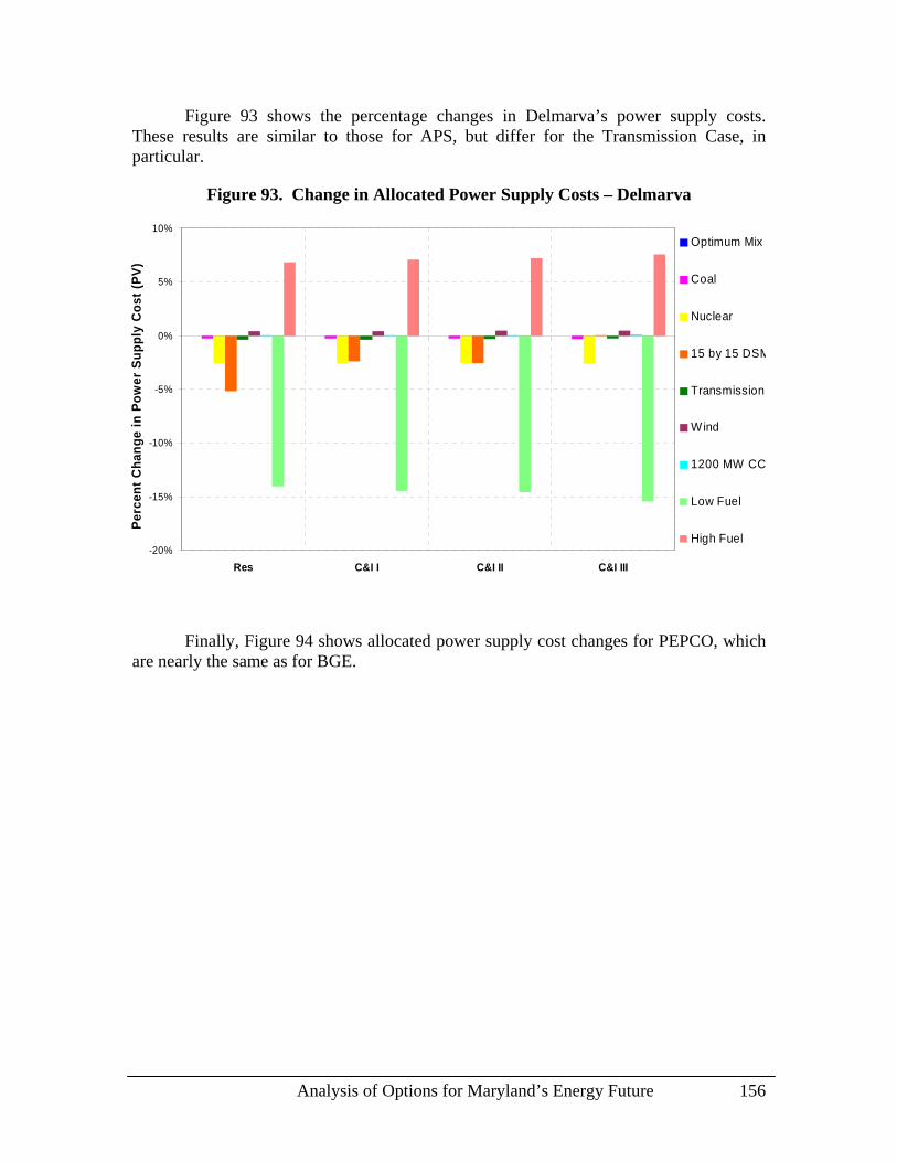
Analysis of Options for Maryland’s Energy Future 156
Figure 93 shows the percentage changes in Delmarva’s power supply costs. These results are similar to those for APS, but differ for the Transmission Case, in particular.
Figure 93. Change in Allocated Power Supply Costs – Delmarva
-20%
-15%
-10%
-5%
0%
5%
10%
Res C&I I C&I II C&I III
Perc
ent C
hang
e in
Pow
er S
uppl
y C
ost (
PV)
Optimum Mix
Coal
Nuclear
15 by 15 DSM
Transmission
Wind
1200 MW CC
Low Fuel
High Fuel
Finally, Figure 94 shows allocated power supply cost changes for PEPCO, which are nearly the same as for BGE.

Analysis of Options for Maryland’s Energy Future 157
Figure 94. Change in Allocated Power Supply Costs – PEPCO
-20%
-15%
-10%
-5%
0%
5%
10%
Res C&I I C&I II C&I III
Perc
ent C
hang
e in
Pow
er S
uppl
y C
ost (
PV)
Optimum Mix
Coal
Nuclear
15 by 15 DSM
Transmission
Wind
1200 MW CC
Low Fuel
High Fuel
V. Conclusions
This analysis quantifies the costs and benefits of various paths that Maryland may take to secure its energy future. Each option has its own set of pros and cons that policy makers will need to evaluate more carefully before choosing the direction forward. Importantly, the State can control most aspects of some alternatives (e.g., regulated utilities’ construction of new gas-fired generation) but plays a more subordinate role with respect to others (e.g., completion of interstate transmission projects). This study provides key data that the State can use to make choices about how it will proceed over the next twenty to assure reliable, affordable electricity.
We began with a baseline Reference Case that we premised on a relatively passive business-as-usual future. Significantly, however, our Reference Case assumes that merchant generators – spurred only by fully functional competitive electricity markets – will build just enough new gas-fired peaking units when and where they are needed to meet expected load growth. The wholesale market’s performance to date in PJM does not support such an optimistic expectation, but this central premise underlies the assumptions we incorporated in the Reference Case regarding reliability and economics over the 20-year study horizon. Moreover, even the relatively modest presumption that DSM programs will achieve 25% of the Governor’s 15 by 15 Initiative’s goals is itself not a foregone conclusion. To the extent electricity demand in Maryland is higher-than-predicted, both wholesale and retail costs are likely to be greater than projected. Thus, the Reference Case may require substantial State action to achieve these baseline levels of costs and benefits.

Analysis of Options for Maryland’s Energy Future 158
One unmistakable conclusion emerges from our study – for the foreseeable future, the State’s electricity costs will be closely tied to the price of natural gas delivered to power plants in Maryland, and, to a lesser extent, oil. These price variations create by far the most dramatic potential impacts on electric energy costs. Premium fossil fuel prices have been and will undoubtedly continue to be volatile. So long as Maryland is dependant on natural gas or oil to generate electricity, the State will be vulnerable to rising and largely uncontrollable costs.
Within this framework – the Reference Case assumptions and subject to fuel price uncertainty – our quantitative analyses identified clear differences among some of the scenarios that we evaluated. In terms of the present value of all economic costs and benefits over the 20-year span of this study (i.e., the EVA), the Transmission Case, the Nuclear Case, and the DSM Case show the greatest promise. Each of these possible approaches showed a significant positive 20-year benefit of $2.2 billion to $2.9 billion over the Reference Case. Of course, they each also pose risks. The State cannot completely control whether or when a beneficial transmission project will be sited, permitted, financed, and completed. A new nuclear plant may also encounter licensing, financing, design, and construction obstacles that may delay or prevent its operation. The very aggressive DSM programs that will be necessary to achieve ambitious penetration levels have never been implemented on this scale, and the costs associated with the market penetration rates incorporated in the forecast are uncertain. Furthermore, the State may need to make substantial investments for the Nuclear or DSM Cases that could be at risk if the programs do not meet expectations.
Other analyzed options offer potential economic benefits but could create environmental detriments as well. The addition of 1200 MW of gas-fired capacity above the amount needed for reliability can materially reduce Maryland’s energy and capacity charges, but it will not reduce reliance on natural gas. On a purely economic basis, a large, state-of-the-art coal plant could also reduce costs, but concerns about greenhouse gas emissions may preclude that alternative. Similarly, a new transmission project that increases Maryland’s electrical connection with cheaper coal-fired generation to the west may also raise environmental issues about reliance on generation that produces higher quantities of greenhouse gases, i.e., “leakage.”
On the other hand, our study showed that some of the analyzed options do not appear to be economically attractive. The postulated Wind Case – which includes both onshore and offshore wind turbines – produced greater costs than economic benefits. Because 500 MW of wind generation will have only about 103 MW of capacity value, it will impact capacity prices only negligibly and will not significantly lower energy prices. Although onshore wind generation can produce net benefits, the high capital costs of the offshore wind farm that we analyzed more than offset its modest benefits. While the addition of wind generation in Maryland will certainly foster the State’s RPS objectives, the economic impact on both wholesale and retail rates will be negligible. Finally, the Optimum Mix Case has no lasting effect on prices. Because this scenario, like the Reference Case, relies on merchant generation responding to competitive market prices,

Analysis of Options for Maryland’s Energy Future 159
the available supply relative to demand will quickly return to equilibrium, and any price benefits will dissipate.
BGE and PEPCO customers will likely reap most of the benefits from any of the analyzed options. Western Maryland (APS’s service territory) does not suffer from the same transmission constraints as SWMAAC. For most of the analyzed options APS will not be affected as significantly as BGE, PEPCO, and Delmarva. In some instances, APS may be somewhat adversely impacted. Delmarva will benefit from new transmission, but until the current constraints are alleviated, it will not receive much relief from new generation built in the BGE and PEPCO service areas. At the retail level, the most promising resource options can potentially reduce rates for BGE and PEPCO customers by about 5%.
The State will need more intensive evaluation of the most attractive alternatives before it can finally determine the best approach for its energy future. Although we have identified definable costs and benefits associated with the identified options, policy makers should also assess the risks entailed in proceeding with each. Because some choices are not exclusive of others, the State may consider a combination of resources, e.g., aggressive DSM programs that produce more immediate results coupled with longer-term solutions like transmission, new nuclear generation, or a permanent overbuild of gas-fired generation. Further analysis will be required to select the best mix of initiatives that achieves appropriate tradeoffs between risk and reward.