Analysis of non-synchronous trading effects on the pricing ...

Univers

ity of

Cap

e Tow

nAnalysis of non-synchronous trading effects on the pricing of

Exchange Traded ProductsAn empirical analysis of the effects on ETP price volatility that result when the ETP instrument is listed on an exchange that is in a different time zone to that

of the underlying securities basket

Dissertation submitted in fulfilment of the requirements for the degree of Master ofCommerce

Author:Tarryn Valle (student number GDDTAR001)

Supervisor: Associate Professor Ryan Kruger (University of Cape Town)

November 2015

The copyright of this thesis vests in the author. No quotation from it or information derived from it is to be published without full acknowledgement of the source. The thesis is to be used for private study or non-commercial research purposes only.

Published by the University of Cape Town (UCT) in terms of the non-exclusive license granted to UCT by the author.

Univers

ity of

Cap

e Tow

n

i

Declaration

I, Tarryn Sydne Valle, hereby declare that the work on which this dissertation

is based is my original work (except where acknowledgments indicate

otherwise) and that neither the whole work nor any part of it has been, is being

or is to be submitted for another degree in this or any other University. I em-

power the University of Cape Town to reproduce for the purpose of research

either the whole or any portion of the contents in any manner whatsoever.

T S Valle

November 2015

ii

Abstract

Exchange Traded Products (ETPs) have become important members of

the investment universe. They are praised by institutional and retail investors

alike for their low cost, transparency and efficient pricing mechanisms. ETPs

trade much like equity securities but with a unique creation and redemption

mechanism which typically aligns quoted prices with the Net Asset Value

(NAV) of the underlying securities. This dissertation examines a class of ETPs

whose underlying reference basket consists of securities listed on stock ex-

changes operating in a time zone different to the time zone of the ETP instru-

ment itself, and whose currencies of the underlying securities are different to

the currency of the ETP instrument. The ETP instruments reviewed comprise

of the iShares MSCI Country Series and are all listed on the New York Stock

Exchange (NYSE).

The ETPs are classified into three groups depending on the degree of

overlap between the exchange operating times on which their underlying secu-

rities are traded and the exchange operating times of the NYSE. These groups

are non-synchronous for no overlapping hours, partially synchronous for some

overlapping hours and synchronous for overlapping hours.

By assessing a measure of range-based volatility during 15-minute intra-

day intervals throughout the NYSE trading day, an understanding of the vola-

tility profile of these ETPs is determined and analysed. It is found that non-

synchronous ETPs do exhibit a higher relative level of volatility when com-

pared to the partially synchronous group. Within the partially synchronous

group, evidence of a regime-shift is observed during the period when the mar-

ket of the underlying securities transitions from open to closed during the

NYSE trading session.

Another factor observed in the relative volatility profile is the impact of

foreign exchange translation. ETPs with underlying securities priced in an

emerging market currency show higher relative levels of range-based volatili-

ty. However, both emerging market and developed market denominated secu-

iii

rities baskets exhibit relatively higher levels of volatility during the opening

and closing periods of the US trading day.

The results point to the need for caution and understanding of the under-

lying reference basket when transacting in these ETPs as investors may inad-

vertently transact at a price which does not reflect the fair-market value of the

underlying securities basket due to price distortions as a result of volatility.

iv

Acknowledgements

I am very appreciative of the input and guidance of Associate Professor

Ryan Kruger, my supervisor. He not only assisted greatly in shaping the anal-

ysis work presented, but also very willingly went more than the extra mile to

smooth a path through the various bureaucratic hurdles ensuring I could regis-

ter as a Masters student. He was also instrumental in securing the required

data and statistical software required – thank you. Thanks also to Associate

Professor Iain MacDonald who effortlessly packaged my statistical conun-

drum into a series of logical questions to help me determine the correct statis-

tical approach to take.

Most importantly, I wish to acknowledge the role that my family has

played in making the completion of this dissertation possible. Aside from

missing me during traditional working hours, my young children, Angelina

and Raffa, have had to miss me on numerous weekends too. This was made

possible only by the incredible support and care of my husband Marco who

understood my desire to undertake a project of this magnitude.

Thank you too to my parents. Dad, I have a far better appreciation of

your impressive academic credentials and Mom, thank you for your unfailing

belief and support in all my endeavours.

Together my support team, both at UCT and at home made this work

possible. Thank you all.

v

Contents

1 Introduction .......................................................................................... 1

2 An Overview of Exchange Traded Products ...................................... 3

2.1 History of the ETP Industry ............................................................................. 3

2.2 Exchange Traded Product Key Features .......................................................... 5

2.2.1 Portfolio as a Stock ......................................................................................................... 5 2.2.2 Defined Portfolio Constituents ........................................................................................ 6 2.2.3 Creation and Redemption Process ................................................................................... 7

2.2.4 Low Cost ......................................................................................................................... 7 2.2.5 Intraday Pricing ............................................................................................................... 9 2.2.6 Derivatives ...................................................................................................................... 9

2.3 Exchange Traded Product Pricing Mechanisms ............................................... 9

2.3.1 Industry Participants...................................................................................................... 10 2.3.2 Creation and Redemption .............................................................................................. 12 2.3.3 Premiums and Discounts ............................................................................................... 12 2.3.4 ETP Price Volatility ...................................................................................................... 13

3 Dual and Cross-listed Instruments.................................................... 14

3.1 Introduction to Dual and Cross-listed Instruments ......................................... 14

3.2 Price Discovery .............................................................................................. 15

3.2.1 Equity Security Price Discovery ................................................................................... 15 3.2.2 ETP Price Discovery ..................................................................................................... 17 3.2.3 Comments on Price Discovery ...................................................................................... 19

4 Security Price Volatility ..................................................................... 20

4.1 Introduction to Volatility ................................................................................ 20

4.2 Range-based Volatility ................................................................................... 21

4.3 Efficiency of Range-based Volatility Estimators ........................................... 24

4.4 Intraday Volatility Patterns ............................................................................ 25

5 Data ...................................................................................................... 28

5.1 MSCI Indices ................................................................................................. 28

5.1.1 MSCI Index Construction Methodology ....................................................................... 28

5.2 iShares MSCI Country Series......................................................................... 29

5.3 ETP Data ........................................................................................................ 30

5.4 Foreign Exchange Data .................................................................................. 35

5.5 Global Exchange Hours ................................................................................. 38

vi

6 Empirical Analysis .............................................................................. 40

6.1 Methodology .................................................................................................. 40

6.2 Range-based Volatility Computations ............................................................ 40

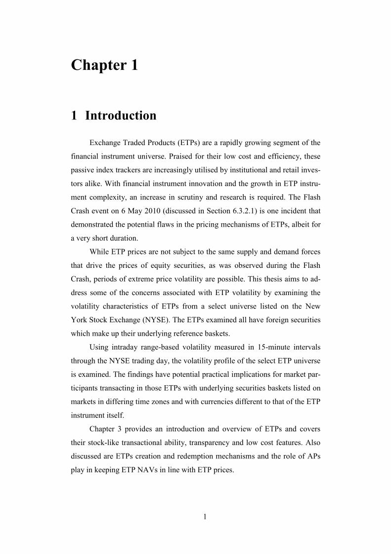
6.3 Initial Data Analysis ....................................................................................... 42

6.3.1 Visual Analysis - Intraday Pattern ................................................................................. 42 6.3.2 Apparent Anomaly at 2:45pm to 3:00pm ...................................................................... 43 6.3.3 Data Adjustment ........................................................................................................... 45

6.4 Data Profile and Testing ................................................................................. 46

6.4.1 Descriptive Statistics ..................................................................................................... 46 6.4.2 Characteristics of the Data Distribution ........................................................................ 47

6.4.3 Testing for Normality .................................................................................................... 48 6.4.4 Testing for Stationarity.................................................................................................. 51 6.4.5 Conclusions from Stationarity Testing .......................................................................... 59

6.5 Preparation for Statistical Analysis ................................................................ 60

6.5.1 Non-Parametric Tests .................................................................................................... 61

6.6 Statistical Analysis ......................................................................................... 63

6.6.1 Initial Statistical Analysis .............................................................................................. 63 6.6.2 Results of the Wilcoxon Signed Rank Test ................................................................... 69

7 Partially Synchronous ETPs .............................................................. 77

7.1 European Market Closing ............................................................................... 77

7.1.1 Results of the Wilcoxon Signed Rank Test – Partially synchronous ETPs .................... 78 7.1.2 Discussion Around Increased Volatility ........................................................................ 80

8 The Impact of Foreign Exchange ...................................................... 83

8.1 Range-based Volatility Computations ............................................................ 83

8.2 Local Currency ETP Prices ............................................................................ 85

8.3 Intraday Volatility Profile in Currency of Underlying Basket ....................... 85

8.3.1 Assessment of the Volatility Difference ........................................................................ 89

9 Conclusion ........................................................................................... 94

Bibliography ................................................................................................... 96

Appendix A ................................................................................................... 101

A.1 Shapiro-Wilk Test Statistics ............................................................................... 101

A.2 Jarque-Bera Test Statistics ................................................................................. 104

Appendix B ................................................................................................... 109

B.1 ADF Test Statistics ............................................................................................. 109

B.2 Phillips-Perron Test Statistics ............................................................................ 113

vii

B.3 KPSS Test Statistics ........................................................................................... 117

Appendix C ................................................................................................... 122

viii

List of Figures

Figure 1: Relationship between ETP Participants .................................................................... 11

Figure 2: Global Exchange Hours in Eastern Standard Time ................................................... 39

Figure 3: Range-based Volatility Measure of Select ETPs - Jan 2006 to Jul 2014 .................. 43

Figure 4: Range-based Volatility Measure of Select ETPs - Jan 2006 to Jul 2014 Excluding

Flash Crash ......................................................................................................................... 46

Figure 5: Range-based Volatility for Select ETPs - Jan 2006 to July 2014 - Aggregated Data 53

Figure 6: Box Plot for All ETPs for Each 15-minute Intraday Interval .................................... 64

Figure 7: Non-synchronous ETPs - Percentage Observations Above and Below United States

ETP Median ........................................................................................................................ 70

Figure 8: Partially synchronous ETPs - Percentage Observations Above and Below United

States ETP Median.............................................................................................................. 71

Figure 9: Synchronous ETPs - Percentage Observations Above and Below United States ETP

Median ................................................................................................................................ 72

Figure 10: Range-based Volatility of Partially Synchronous ETPs Before, During and After

European Market Close ...................................................................................................... 82

Figure 11: Range-based Volatility Measure of Foreign Exchange Pairs - Sep 2009 to Jul 2014

............................................................................................................................................ 83

Figure 12: Non-Synchronous ETP Range-based Volatility - USD versus Underlying Currency

- Sep 2009 to Jul 2014 ........................................................................................................ 86

Figure 13: Partially Synchronous ETP Range-based Volatility - USD versus Underlying

Currency - Sep 2009 to Jul 2014 ......................................................................................... 87

Figure 14: Synchronous ETP Range-based Volatility - USD versus Underlying Currency - Sep

2009 to Jul 2014 .................................................................................................................. 88

ix

List of Tables

Table 1: Descriptive Data for All ETPs - Jan 2006 to Jul 2014 ............................................... 31

Table 2: Descriptive Data for Foreign Exchange Pairs versus United State Dollar - Sep 2009 to

Jul 2014 ............................................................................................................................... 36

Table 3: Descriptive Statistics of Range-Based Volatility for all ETPs - Jan 2006 to Jul 2014 -

Aggregated Data ................................................................................................................. 47

Table 4: Average Percentages Above and Below IVV Median per ETP ................................. 73

Table 5: Percent Observations Above and Below Median Value in Interval 11:00am to

11:15am Compared with Median in Interval 11:15am to 11:30am for Partially

Synchronous ETPs .............................................................................................................. 79


11:45am Compared with Median in Interval 11:45am to 12:00pm for Partially

Synchronous ETPs .............................................................................................................. 79

Table 7: Average Difference in Range-based Volatility by Time Zone ................................... 89

Table 8: Average Difference in Range-based Volatility by Country Classification ................. 91

Table 9: Average Difference in Range-based Volatility in First and Last 30 Minutes versus

Remainder of Trading Day by Country Classification........................................................ 92

Appendix Table 1: Shapiro-Wilk Test Results for Non-Synchronous ETPs – Jan 2006 to Jul

2014 – Non-Aggregated Data ........................................................................................... 101

Appendix Table 2: Shapiro-Wilk Test Results for Partially Synchronous ETPs – Jan 2006 to

Jul 2014 – Non-Aggregated Data ..................................................................................... 102

Appendix Table 3: Shapiro-Wilk Test Results for Synchronous ETPs – Jan 2006 to Jul 2014 –

Non-Aggregated Data ....................................................................................................... 103

Appendix Table 4: Jarque-Bera Test Results for Non-Synchronous ETPs – Jan 2006 to Jul


Appendix Table 5: Jarque-Bera Test Results for Partially Synchronous ETPs – Jan 2006 to Jul


Appendix Table 6: Jarque-Bera Test Results for Synchronous ETPs – Jan 2006 to Jul 2014 –

Non-Aggregated Data ....................................................................................................... 108

Appendix Table 7: ADF Test Results for Non-Synchronous ETPs – Jan 2006 to Jul 2014 –

Aggregated Data ............................................................................................................... 109

Appendix Table 8: ADF Test Results for Partially Synchronous ETPs – Jan 2006 to Jul 2014 –

Aggregated Data ............................................................................................................... 110

Appendix Table 9: ADF Test Results for Synchronous ETPs – Jan 2006 to Jul 2014 –

Aggregated Data ............................................................................................................... 112

x

Appendix Table 10: Phillips-Perron Test Results for Non-Synchronous ETPs – Jan 2006 to Jul

2014 – Aggregated Data ................................................................................................... 113

Appendix Table 11: Phillips-Perron Test Results for Partially Synchronous ETPs – Jan 2006

to Jul 2014 – Aggregated Data.......................................................................................... 114

Appendix Table 12: Phillips-Perron Test Results for Synchronous ETPs – Jan 2006 to Jul

2014 – Aggregated Data ................................................................................................... 116

Appendix Table 13: KPSS Test Results for Non-Synchronous ETPs – Jan 2006 to Jul 2014 –

Aggregated Data ............................................................................................................... 117

Appendix Table 14: KPSS Test Results for Partially Synchronous ETPs – Jan 2006 to Jul

2014 – Aggregated Data ................................................................................................... 119

Appendix Table 15: KPSS Test Results for Synchronous ETPs – Jan 2006 to Jul 2014 –

Aggregated Data ............................................................................................................... 121

Appendix Table 16: Descriptive Statistics Partially Synchronous ETPs: 11:00am to 11:15am

.......................................................................................................................................... 122

Appendix Table 17: Results of Wilcoxon Signed Rank Test for Partially Synchronous ETPs:

11:00am to 11:15am compared with 11:15am to 11:30am ............................................... 122

Appendix Table 18: Descriptive Statistics Partially Synchronous ETPs: 11:30am to 11:45am

.......................................................................................................................................... 124

Appendix Table 19: Results of Wilcoxon Signed Rank Test for Partially Synchronous ETPs:

11:30am to 11:45am compared with 11:45am to 12:00pm............................................... 125

1

Chapter 1

1 Introduction

Exchange Traded Products (ETPs) are a rapidly growing segment of the

financial instrument universe. Praised for their low cost and efficiency, these

passive index trackers are increasingly utilised by institutional and retail inves-

tors alike. With financial instrument innovation and the growth in ETP instru-

ment complexity, an increase in scrutiny and research is required. The Flash

Crash event on 6 May 2010 (discussed in Section 6.3.2.1) is one incident that

demonstrated the potential flaws in the pricing mechanisms of ETPs, albeit for

a very short duration.

While ETP prices are not subject to the same supply and demand forces

that drive the prices of equity securities, as was observed during the Flash

Crash, periods of extreme price volatility are possible. This thesis aims to ad-

dress some of the concerns associated with ETP volatility by examining the

volatility characteristics of ETPs from a select universe listed on the New

York Stock Exchange (NYSE). The ETPs examined all have foreign securities

which make up their underlying reference baskets.

Using intraday range-based volatility measured in 15-minute intervals

through the NYSE trading day, the volatility profile of the select ETP universe

is examined. The findings have potential practical implications for market par-

ticipants transacting in those ETPs with underlying securities baskets listed on

markets in differing time zones and with currencies different to that of the ETP

instrument itself.

Chapter 3 provides an introduction and overview of ETPs and covers

their stock-like transactional ability, transparency and low cost features. Also

discussed are ETPs creation and redemption mechanisms and the role of APs

play in keeping ETP NAVs in line with ETP prices.

2

In cases where the underlying securities basket of an ETP is made up of

foreign securities, ETPs are not dissimilar in nature to dual or cross-listed se-

curities. Chapter 3 discusses price discovery mechanisms for cross-listed equi-

ty securities and ETPs with foreign security underlying baskets.

Chapter 4 introduces volatility which is a critical subject for market

practitioners and focusses on range-based volatility as a measure. Also dis-

cussed are intraday volatility patterns where systematic variance in trading

patterns over the trading day produces distinct volatility shapes.

The prior research of Chapters 2, 3 and 4 is applied to the dataset as de-

scribed in Chapter 5. In order to understand the distribution profile of the

range-based volatility measures, analysis and testing is conducted in Chapter

6. Chapter 7 examines the partially synchronous ETPs in additional detail. The

final element of this study is covered in Chapter 8 where the impact of foreign

exchange is assessed.

3

Chapter 2

2 An Overview of Exchange Traded Prod-

ucts

2.1 History of the ETP Industry

Research work and media articles covering the Exchange-Traded Prod-

uct (ETP) industry typically highlight statistics on the rapid growth of these

innovative instruments. There has been a proliferation of products and a gath-

ering of assets under management by ETP providers. The terms Exchange

Traded product (ETP) and Exchange Traded Fund (ETF) are used to describe

exchange traded investment vehicles. Not all ETPs are funds and ETFs are a

subset of the broader ETP universe.

The early building blocks for ETPs came with the implementation of

electronic order technology on the New York Stock Exchange (NYSE) and the

American Stock Exchange (Amex). Together with the capabilities of large

investment banks to execute programme trades, these changes made it possible

for investors to pursue futures and stocks arbitrage strategies. Programme or

portfolio trades as they became known, attempted to take advantage of pricing

discrepancies which arose between the newly created S&P500 futures

contracts traded on the Chicago Mercantile Exchange (CME) and the

underlying stocks in the S&P 500 index. Settlement of the CME futures, either

long or short, could be undertaken in stock, in an exchange of futures for phys-

icals (EFP) (Gastineau, 2001).

Typically, it was large investors making use of EFP trades and smaller

institutions and retail investors sought a Securities and Exchange Commission

(SEC) regulated product that could deliver the payoff profile of an EFP trade.

Index Participation Shares (IPS) mirroring the S&P 500 were introduced and

4

began trading on Amex and the Philadelphia Stock Exchange in 1989.

Unfortunately for investor interests, the CME and the Commodity Futures

Trading Commission (CFTC) contested that IPS products were futures

contracts rather than stock-like securities. These entities felt IPS products

should, therefore, trade on a futures exchange and fall under the regulatory

authority of the CFTC. The position of the CME and CFTC was vindicated,

and a federal court found IPS products were indeed futures-like in structure.

The United States product creators remained unsuccessful in their bid to find a

replacement to Index Participation Shares. In Toronto, Canada, Toronto Stock

Exchange Index Participations (TIPs) were successfully introduced and listed

as stock-like instruments.

The immediately unique feature of the TIPs suite of products was their

expense ratio. Script lending was possible, allowing the trustee of the TIPs

product to loan out the underlying securities in the basket, passing those reve-

nue streams back to the product investors. Despite the attractiveness to

investors who at times experienced a negative expense ratio (they received

payment for investing in a TIPs product) it was expensive for the exchange

itself. In 2000 the Toronto Stock Exchange (TSE) liquidated the TIPs

portfolios. During this time of product advancement in Canada, two new port-

folio-as-a-security type instruments were being debuted in the United States.

These two products were Supershares and Standard & Poor’s Depository

Receipts (SPDRS). The confusing and complex legal structure detracted from

the Supershares offering and it was ultimately liquidated. The SPDRS prod-

ucts were the resounding winners in the ETP landscape. Amex, who developed

SPDRS, chose to adopt a unit trust structure rather than establishing a costly

mutual fund thus paving the way for low-cost instruments. It took time for in-

vestors to become comfortable and familiar with the then-novel creation and

redemption process, but the asset growth of SPDRS has been exponential.

Another important innovation within the ETP environment came in

March 1996 with the establishment of a series of products known as World

Equity Benchmark Shares (WEBS). These funds, listed on Amex, tracked var-

ious foreign or non-US indices. Foreign stocks made up the underlying hold-

5

ings basket. Barclays Global Investors (BGI), a subsidiary of Barclays plc, es-

tablished WEBS. BGI later changed the name WEBS to the more commonly

known iShares brand. Aside from being the first to track indices comprised of

foreign stocks, BGI took the decision to structure their WEBS offering as a

mutual fund rather than a unit trust as SPDRS had done. The flexibility of a

mutual fund structure when creating a large number of similar products out-

weighed the additional establishment costs of the structure.

While iShares and SPDRS were the ETP founding members, as at the

end of June 2014, there were 219 ETP providers with 5 359 ETPs and 10 401

listings globally (Fuhr, 2014). The industry has experienced a period of expo-

nential growth and ETPs have established themselves as mainstream products

within the institutional and retail investor environment globally.

2.2 Exchange Traded Product Key Features

If the growth in assets under management is a measure of financial

product success, then ETPs have undoubtedly been vastly successful. In 2000,

ETPs globally comprised assets of US$79 billion which over the last 14 years

have grown to US$2 640 billion (Fuhr, 2014). To attract such sustained asset

flows over the period, there are clearly unique attributes that ETPs possess that

have drawn retail and institutional investors alike.

2.2.1 Portfolio as a Stock The foundations for ETPs came about through the desire to trade a refer-

ence basket or portfolio in a single transaction. Initially, the ability to take

advantage of arbitrage opportunities between the futures and underlying

physical basket created demand for ETPs. Increasingly though, the “portfolio

as a stock” concept allowed small retail investors and large institutional

investors to gain market representation without the high transaction costs and

administrative load of attempting to hold each underlying stock in a particular

index. While constituents of a major index like the S&P 500 are all relatively

liquid, the same is not true of more niche sections of the market. The ease with

6

which exposure is gained to specific market segments through a single stock-

like transaction is very appealing to investors.

2.2.2 Defined Portfolio Constituents ETPs typically track a reference index as evidenced by the first genera-

tion ETPs that tracked headline indices like the S&P 500, NASDAQ and the

EuroStoxx 50. Index tracking came about due to the exemptive relief from

various provisions of the Investment Company Act of 1940 granted by the

SEC in 1993 to allow ETPs to track designated indices (Investment Company

Institute, 2014). Investors, therefore, have a relatively good appreciation of the

underlying constituents and the likely payoff profile of these products.

Mutual fund management is typically performed on a discretionary ba-

sis. Investors may have a reasonable idea of the likely mutual fund portfolio

holdings based on the categorisation and mandate of the mutual fund,

however, managers seek to add value by allocating away from a benchmark or

index. Thus, investors do not enjoy the same level of certainty on the mutual

fund constituents, likely performance profile and level of exposure to a partic-

ular segment that they have with ETPs.

Current ETPs have become far more sophisticated in their offering,

thanks to further exemptive relief granted by the SEC in 2008. Over and above

tracking typical market capitalisation weighted indices, there can now be an

element of discretion to their underlying reference basket or a rules-based trad-

ing methodology that switches the underlying instruments dependent on mar-

ket conditions. These “enhanced” indices have developed as investor appetite

for new products has grown. ETPs providers have responded, giving investors

the ability to gain exposure to derivative type instruments efficiently. These

include futures on certain commodities or volatility indices or specialist or il-

liquid instruments such as emerging market debt or emerging market real es-

tate. The ETP providers have also sought to divide the market into increasing-

ly finer slices providing the ability to have exposure to very niche segments

like energy focused master limited partnerships or Japanese healthcare.

7

New generation ETPs allow investors to have certainty about the

underlying constituents in their selected product, but with the ability to access

more complex parts of the financial instrument universe that were once the

preserve of institutional and hedge fund managers alone.

2.2.3 Creation and Redemption Process Although ETPs trade through the day in a similar manner to individual

equity securities, the creation and redemption process is a key differentiating

factor. The mechanics of creation and redemption is discussed in Section 2.3.

ETP managers have the ability to absorb the fluctuating demand and supply

for their shares without those demand and supply forces impacting the ETP

price. Large flows to an open-ended mutual fund can significantly hamper its

subsequent performance due to flow-induced trading costs (Guedj & Huang,

2008). ETP performance is not affected by monetary flows.

Following a placement of a large order for a particular ETP, if there are

insufficient shares available, the Authorised Participant (AP) can create addi-

tional shares to meet the demand. In the case of an equity which typically has

a finite number of shares available, a large order or increased demand will

drive up the price of the equity security. The converse it true in the case of a

redemption order.

2.2.4 Low Cost As discussed in Section 2.1, the TIPs traded on the Toronto Stock Ex-

change had periods of not only low, but often negative expensive ratios. The

TIPs set the scene for one of the distinguishing features of ETPs, namely low

cost.

2.2.4.1 Total Expense Ratio

The Total Expense Ratio is a measure of the costs associated with the

management and operation of an investment product divided by the assets of

the investment product. Expenses typically include management or perfor-

mance fees, trading costs, administration fees and legal and audit fees.

8

ETPs tend to have lower management fees and administrative and trad-

ing costs than mutual funds. They also don’t include any up-front or redemp-

tion fees and there is no minimum investment size, unlike the mutual fund in-

dustry. A large portion of mutual fund fees are for shareholder accounting ser-

vices; a net cash flow of a mutual fund through the subscription or redemption

of units triggers purchases or sales of the underlying holdings. These transac-

tions require record keeping and validation.

ETP managers also engage in the practice of securities lending. The ETP

manager will lend out the securities to a large institution for a period. The bor-

rower of the securities over-collateralises the position typically in cash and the

ETP manager earns a return on this collateral. This additional revenue is used

to offset some of the ETP expenses benefitting ETP investors.

2.2.4.2 Tax Efficiency

When a mutual fund rebalances its underlying security holdings, the re-

sultant net capital gain is distributed to the investors in the fund on a quarterly

basis. When rebalancing occurs within an ETP, there are no immediate tax ef-

fects for the investors and investors only realise capital gains when they sell

the ETP shares.

The in-kind redemption mechanism of ETPs enables them to meet

redemption requests without the need to sell portfolio securities. As a result,

redemptions from the ETP will generally not have any tax impact on the non-

redeeming shareholders (Rosella & Pugliese, 2006).

2.2.4.3 Spreads

When the shares of an ETP first begin trading on an exchange, the bid-

ask spread will typically reflect the average spread of the ETP’s underlying

holdings (BlackRock Inc, 2013). Over time, this spread tends to narrow sub-

stantially, reflecting the liquidity of the ETP itself. Thus, the cost of gaining

exposure to the underlying basket of securities is far lower than the average

spread or cost of obtaining the securities directly.

9

2.2.4.4 Trading costs

Long-term investors in mutual funds subsidise trading costs by investors

who frequently trade (Hamm, 2010). However, in the case of ETPs, only the

investor transacting in the ETP carries the cost.

2.2.5 Intraday Pricing ETPs trade continuously through the day at prices determined by intra-

day supply and demand rather than at the calculated net asset value (NAV)

(Engle & Sarkar, 2002). When investors wish to participate in a mutual fund,

they purchase the fund at an end-of-day NAV – intraday pricing is unavaila-

ble. While the closing NAV for ETPs is, like mutual funds, only calculated at

the end of the day, throughout the trading day an indicative NAV is provided

in 15-second intervals. The intraday NAV is referred to as the iNAV or indica-

tive optimised portfolio value (IOPV).

The ability to trade intraday provides ETPs with a liquidity advantage

over mutual funds. Investors can exit or enter a trade at any time during a trad-

ing session to capitalise on a perceived transactional opportunity.

2.2.6 Derivatives As ETPs possess many of the characteristics of equities rather than mu-

tual funds, derivative instruments can be created with the ETP as the underly-

ing asset. This feature allows for the creation ETP derivatives in the form of

options and futures. These derivatives enable investors to take leveraged or

hedging positions on ETPs. ETPs themselves can also be shorted, enabling

investors to construct a payoff profile of their choosing.

2.3 Exchange Traded Product Pricing Mechanisms

As mentioned in Section 2.2.3 ETPs have a unique creation and redemp-

tion mechanism that serves to keep ETP prices trading relatively closely to

their net asset value. The mechanics of this pricing process involve many in-

10

dustry participants to ensure the end investor has confidence that the quoted

price is a true representation of the value of the underlying basket.

2.3.1 Industry Participants There are many participants in the ETP production cycle, each fulfilling

various functions within the trading and pricing process. ETP managers or

sponsors conceptualise the ETP. ETP sponsors are typically large asset man-

agers who elect to provide a non-actively managed or rules-based investment

product tracking a particular reference basket. The reference baskets are creat-

ed by index providers, some are established primary indices tracking various

global exchanges while other reference baskets track indices developed specif-

ically for the ETP provider. These bespoke indices allow the ETP provider to

offer a wide variety of potential products.

Once an ETP has been conceptualised and obtained appropriate regula-

tory approval, its shares begin to trade on an exchange.

2.3.1.1 Primary Market Participants

Within the ETP trading process, an Authorised Participant (AP) plays a

significant role. The AP is typically a large institutional investor with the abil-

ity to settle large share transactions with the ETP sponsor. At the commence-

ment of the trading of a new ETP, the AP will deliver the underlying basket of

securities to the ETP sponsor and receive shares of the ETP in exchange. This

initial delivery is a primary market transaction undertaken between the AP and

the ETP manager; regular institutional and retail investors do not deal directly

with the ETP sponsor. While APs are appointed and approved by the ETP

sponsor, they do not receive compensation from the ETP sponsor. The costs of

purchasing, holding and delivering the underlying reference basket securities

are borne exclusively by the AP and the ETP sponsor or regular investors do

not incur these costs. APs undertake the role because it generates profit

through arbitrage opportunities and provides a useful component to their busi-

ness. APs continue to deal with the ETP sponsor as the agent to create and re-

deem ETP shares in the primary market throughout the life of the ETP, meet-

ing secondary market ETP supply and demand requirements.

11

2.3.1.2 Secondary Market Participants

Regular retail and institutional investors, as well as the AP, will transact

in ETP shares in the secondary market. In creating the ability for transactions

to occur, institutions fulfil various roles. Within the secondary market, a Mar-

ket Maker (MM) provides a “two-sided” market. That is, they provide a firm

bid and offer price for a listed security, including ETPs. Market Maker is a

generalised term, and these market-making institutions do not necessarily have

any regulatory or exchange obligations to provide buy and sell prices.

Registered Market Makers (RMMs) are those Market Markers who, as

the name implies, are exchange-registered to provide two-sided quotes for par-

ticular securities listed on that exchange. Exchanges like NYSE Arca and

NASDAQ further differentiate between Registered Market Makers, designat-

ing them Lead Market Makers (LMMs) and Designated Liquidity Providers

(DLPs), respectively.

ETP Shares

ETP Shares Cash

Cash Securities

Cash

ETP Sponsor

Authorised Partici-

pant/Market Maker

Exchange

Creation

Units

Basket of

Securities

Investors

Markets

Primary Market

Secondary Market

Figure 1: Relationship between ETP Participants

12

2.3.2 Creation and Redemption ETPs issue and redeem shares in blocks of a minimum size. These

blocks are referred to as Creation Units and only the Authorised Participant

(AP) can create or redeem them in the primary market. Creation Units typical-

ly comprise 25,000 to 50,000 shares or US$5,000,000. The AP will receive

either cash or the basket of underlying securities that make up the ETP from

the ETP sponsor. The receipt of physical securities is an “in kind” transaction.

The constituents of the “in kind” basket are published at the close of each trad-

ing day. APs can buy and sell ETP shares in the secondary market, or transact

directly with the ETP sponsor. Although the creation and redemption of shares

occurs at the end of the trading day, intraday the AP will sell the more

expensive asset (either the ETP shares if the ETP is trading at a premium to

NAV or the underlying basket constituents) and buy the cheaper asset. At the

end of the trading day, the AP can simply unwind its position by creating or

redeeming shares at NAV should it wish to do so. There are of course costs

associated with the transfer, and the AP will incorporate those costs into the

computation of arbitrage profit prior to embarking on the transaction.

2.3.3 Premiums and Discounts Premiums and discounts arise when the ETP price is either above or be-

low the ETP NAV. ETPs with illiquid securities in their underlying baskets are

more likely to trade at a price different to their NAV. Due to the illiquidity of

the underlying securities, APs may find it more difficult and expensive to cre-

ate the underlying security basket for an in-kind creation or redemption. The

arbitrage mechanism is, therefore, less efficient.

Together with the illiquidity of the underlying securities, if the AP has

difficulty in determining the NAV of the underlying securities, this introduces

an additional element of risk in the arbitrage transaction. International securi-

ties traded in different time zones or securities priced in multiple currencies; or

indeed in jurisdictions which restrict security ownership all increase the com-

plexity of the NAV calculation.

13

For non-domestic ETPs, premiums and discounts are observed to be

much larger and more persistent. An explanation for this difference may rest

with the higher cost of creation and redemption for international products

(Engle & Sarkar, 2002). Certain countries will require the payment of taxes

during a share transfer process while in other countries there are restrictions on

the ownership of securities by foreigners. In these cases, creations and re-

demptions are cash settled with a domestic trustee holding the securities. The

delivery mechanisms are, therefore, slower and more costly (Engle & Sarkar,

2006).

Positive premiums on ETPs lead to more share creation, and vice versa

for negative premiums, indicating arbitragers are actively using the ETP share

creation and redemption process to trade against these mispricings (Petajisto,

2013). Results using end-of-day data indicate that these premiums are lacking

in persistence and vanish over two successive trading days (Rompotis, 2010).

The lack of premium persistance confirms that ETPs are efficient investment

vehicles for investors with medium to longer-term investment time horizons.

2.3.4 ETP Price Volatility As ETPs trade on a stock exchange in the same manner as a listed

financial security, the price behaviour of the ETP instrument is volatile

throughout the trading day. This volatility is due to the prevailing demand and

supply for the instrument and information flow creating differing expectations

about the potential future price. This price volatility occurs irrespective of the

creation and redemption mechanisms that serve to keep the ETP price close to

the NAV of the underlying basket and is examined in further detail in Chapter

4.

14

Chapter 3

3 Dual and Cross-listed Instruments

3.1 Introduction to Dual and Cross-listed Instruments

Dual-listed instruments result in the creation of two separate legal enti-

ties that operate as a single business through a legal equalisation agreement.

The respective stock-exchange listings of the two entities are typically in two

different geographic locations, oftentimes motivated by tax advantages to the

shareholders. Additionally, access to diverse capital markets and the associat-

ed market regulations can add to the ability of the company to raise capital.

Cross-listed securities comprise of only one distinct legal entity that has

issued and listed instruments on a primary and sometimes multiple secondary

foreign exchanges. Firms may choose to cross-list to participate in geograph-

ically different capital markets in the same way as dual-listed companies.

Cross-listed instruments include American Depository Receipts (ADRs),

European Depository Receipts (EDRs), International Depository Receipts

(IDRs) and Global Registered Shares (GRSs). A depositary bank purchases the

domestic securities and places them with a custodian and issues US Dollar de-

nominated tradeable assets in the form of certificates to create Depository Re-

ceipts which are derivative instruments. The depositary receipts and their do-

mestic underlying securities are not fully fungible; to switch between the two a

conversion fee is typically charged. GRSs are a single class of ordinary share

listed on both the domestic and foreign exchange. Conversion fees do not

apply in switching between the GRS and the domestic stock. As the GRS is

denominated in US Dollars when listed on a US exchange and receives

dividends in US Dollars rather than the domestic currency, GRSs also not fully

fungible.

15

Surveyed institutional investors reflect that they typically view cross-

listed securities as substitutes and make a determination on which instrument

to purchase based on liquidity and transaction costs (Moulton & Wei, 2005).

Although ETPs whose underlying baskets comprise of foreign securities

not listed on the same exchange as the ETP instrument are not strictly

classified as dual or cross-listed, there are definite similarities between the

two. To determine the NAV for the ETP, the price of the underlying assets

needs to be accurately determined. The mechanics of how the underlying

prices of the securities in the reference basket flow through to the ETP during

times when the ETP is trading are analogous to the pricing relationship

between dual or cross-listed stocks on their respective domestic and foreign

exchanges. Importantly, like their ADR counterparts, ETP price discrepancies

between the ETP and the underlying basket can be easily arbitraged through

in-kind creation and redemption mechanisms.

3.2 Price Discovery

Price discovery is the term given to the determination of the price of an

asset through the demand-supply interactions of buyers and sellers. Price dis-

covery is also defined as the search for the equilibrium price and is an im-

portant function of an exchange. In the case of dual- and cross-listed securi-

ties, prior research has centred on the determination of the flow of information

or liquidity between the domestic and foreign exchanges. Previous work large-

ly indicates that for equity securities, price discovery occurs primarily in the

domestic or home market of the security.

3.2.1 Equity Security Price Discovery Chan, Fong, Kho and Stulz (1996) investigated the intraday patterns of

European and Japanese dual-listed stocks trading on the NYSE and AMEX.

Due to partially overlapping exchange trading hours, public information from

European stocks diminishes mid-way through the US trading day as European

markets close. The arrival of public information from Japanese stocks is uni-

16

form and low through the US trading day as Japanese markets are closed

throughout the US trading session (Chan, et al., 1996). Following from their

analysis, it would appear that US based investors transact in the market on the

basis of information accumulated from the previous US market close to the

next day’s opening. This accumulated information is largest for Japanese

stocks that have had a full trading day prior to US open and less for European

stocks since there is half a trading day between US market close and open.

This notion of reaction to accumulated information provides an explanation

for their finding that Japanese and European stocks are most volatile during

the US morning trading session.

Eun and Sabherwal (2003) examined a sample of Canadian stocks listed

on both the Toronto Stock Exchange (TSE) and the NYSE, Amex or

NASDAQ. Their objective was to examine the extent to which the NYSE

listed security contributes to the price discovery of the TSE listed security.

They suggested that the domestic exchange is likely to contribute meaningful-

ly to the price discovery as material information originates in the home mar-

ket. However, they also noted that as US exchanges are typically the largest

and most liquid globally, they are also likely to contribute to price discovery.

As Canadian and US market hours overlap, their findings were potentially dif-

ferent from other work conducted in dual or cross-listed Asian and European

securities. They found that the US markets contribute to the price discovery of

the Canadian listed securities but for the majority of stocks, the TSE is domi-

nant (Eun & Sabherwal, 2003).

Grammig, Melvin and Schlag (2005) reviewed three German stocks

listed on the Frankfurt Exchange (XETRA) and their NYSE listed ADR coun-

terparts. They looked specifically at high-frequency data during overlapping

trading hours between the two markets to determine where price discovery oc-

curs. Their empirical results support the assertion that price discovery occurs

in the domestic market for the three stocks reviewed rather than the foreign

market. A secondary examination was to determine how the security prices

reacted to an exchange rate shock. The domestic securities are denominated in

Euros while the foreign securities are US Dollar denominated. They found that

17

the foreign instruments bore almost all the price adjustment to an exchange

rate shock – the ADRs re-priced, rather than the domestic stocks. These find-

ings add support to the opinion that price discovery of cross or dual-listed

stocks occurs principally in the home market of those stocks (Grammig, et al.,

2005).

Agarwal, Liu and Rhee (2007) examined a sample of stocks that trade on

both the Hong Kong Exchange (HKEx) and the London Stock Exchange

(LSE). The focus of their paper addressed the idea that the foreign market in-

fluenced the pricing in the domestic market. This finding would mean that the

price information flow is perhaps both from domestic to foreign and from for-

eign to domestic. They found the setting of LSE opening prices benchmarked

against the HKEx close, meaning the LSE market played only a limited role in

the price discovery of HKEx stocks. London closing prices were not

incorporated into HKEx opening. LSE (foreign) pricing would appear to play

an insignificant role in the generation of price information for the HKEx (do-

mestic) pricing (Agarwal, et al., 2007). They suggested that trading of these

stocks on the LSE is liquidity-driven rather than information-driven.

3.2.2 ETP Price Discovery In an examination of price discovery in international iShares Country

ETPs listed on the NYSE, Tse and Martinez (2007) reviewed the variance of

daytime returns and overnight returns. They suggested that if noise trading or

private information drove volatility, then higher volatility would result from

increased trading activity. If, however, volatility was due to the flow of infor-

mation in domestic markets, then the overnight variance would be greater than

the daytime variance. They found that the the daytime deviation for both Asian

and European ETPs was smaller than overnight deviation with the converse

being true for ETPs tracking the American market. Here they found the

daytime variance was greater than the overnight variance. They concluded that

the volatility of these ETP instruments was driven primarily by public infor-

mation released during the respective domestic market sessions (Tse &

Martinez, 2007).

18

Hughen and Mathew (2009) reviewed Closed Ended Funds (CEFs) and

ETPs trading in the US whose underlying baskets represented non-US securi-

ties. Their ETP sample also utilised the international iShares Country ETPs

while their CEF universe consisted of those funds classified as world equity

and which published a daily NAV. They analysed the transmission of price

changes between the value of the underlying security baskets (NAV) and the

price of the ETP and CEF instruments listed on US exchanges. They also test-

ed the sensitivity of ETP and CEF prices to the daily returns of the US market.

They found that shocks to the NAV of ETP and CEF instruments had a posi-

tive effect on prices for several days with the affected period being longer for

CEFs than ETPs. They found an overreaction to US stock market returns with

both ETPs and CEFs exhibiting a positive relation with the concurrent returns

on the S&P 500 (Hughen & Mathew, 2009).

Levy and Lieberman (2013) studied the price formation process of inter-

national iShares country ETPs listed on the NYSE. Their findings suggested a

changing relationship in the factors contributing to the ETP price. This rela-

tionship was dependent on whether the domestic market of the underlying

constituents was open or closed during the US trading session. They found that

when domestic markets were open, ETP returns were driven predominantly by

NAV returns, in other words, the pricing of the underlying securities listed on

the home market. However, when the underlying domestic market was closed,

they found the returns of the S&P 500 dominated ETP returns. By examining

intraday data in 15-minute time intervals throughout the US trading day, they

isolated the period when European markets closed during the US morning and

examined the principle ETP price drivers before and after this European

closing event. They determined that there was a “regime shift” which occurred

for European ETPs. The effect of the S&P 500 on European ETP pricing in-

creased significantly after the European market close. They also found that the

effect that the S&P 500 returns had on those ETPs whose domestic market was

closed throughout the US trading session exceeded the effect it had on the

foreign indices which the ETP products track. The ultimate conclusion was an

19

overreaction to US market returns during non-overlapping trading hours (Levy

& Lieberman, 2013).

3.2.3 Comments on Price Discovery The prior literature focussed on the price discovery of dual or cross-

listed equity securities seems to suggest a dominance of the home or domestic

market in driving the price behaviour of the security. Equity security research

has focussed on intraday periods and covers overlapping and non-overlapping

market trading periods. Irrespective of whether liquidity traders or information

traders drive price discovery, it seems home markets take the lead in price

equilibrium.

In reviewing the literature on ETP price discovery, it should be noted

that both Tse and Martinez (2007) and Hughen and Mathew (2009) did not use

intraday segmented data. While Tse and Martinez (2007) examined overnight

and daytime variance, they did not review periods within the trading day and

Hughen and Mathew (2009) focussed on daily returns only. Their conclusions

were similar to the general research findings on equity securities the home or

domestic market is dominant in driving ETP prices. Levy and Lieberman

(2013) did examine ETP data intraday and they found evidence that the domi-

nance of the domestic market varied dependant on whether that domestic mar-

ket was open during the US trading session or not. The intraday review of Eu-

ropean ETPs allowed them to isolate an intraday regime shift and find a de-

pendence on S&P 500 returns as a price driver. This finding is different from

the prior work and suggests that further analysis at more granular intraday pe-

riods is required to reach a full understanding of the characteristics of ETPs

with international underlying securities in their reference basket.

20

Chapter 4

4 Security Price Volatility

4.1 Introduction to Volatility

From a financial practitioner’s perspective, volatility is a critical subject

as option and derivative pricing models incorporate a measure of volatility, as

do risk and asset pricing models and asset allocation and portfolio construction

techniques. Most simply, historical volatility can be computed as the standard

deviation of daily returns using close-to-close prices over a particular period.

The implicit assumption in this computation is that volatility remains constant

over the period which is unrealistic. The calculation of volatility is rendered

more complex by the measurement period as data measured over shorter inter-

vals tend to display different characteristics to that measured over longer peri-

ods.

Measuring volatility using high-frequency data is the subject of much

recent research. Anderson, et al. (2001) propose the usage of a new volatility

measure termed “realised volatility”. The daily realised volatility is computed

by summing the intraday squared returns. Through the use of high-frequency

data, the realised volatility computation converges to the underlying volatility.

Various researchers have found that in practise, the microstructure noise

effects, like a bid-ask bounce begins to distort returns at very high sampling

frequencies. This distortion leads to realised volatility computations that are

biased and inconsistent (Martens & van Dijk, 2007). The data interval selected

needs to incorporate a balance between the desires for almost continuous data

i.e. very high frequency and the resulting contamination by microstructure ef-

fects (Anderson, et al., 2001).

An alternative to realised volatility computations is to estimate volatility

using trading range data, in other words, open-high-low-close data points. Us-

21

ing additional price range data has been shown to be more efficient than rely-

ing on closing prices alone. Martens and van Dijk (2007) assert that the daily

range as a volatility measure is more robust against the effects of microstruc-

ture noise than realised volatility or variance. They employ a range-based ap-

proach to volatility estimation, and their empirical findings confirm that range

volatility estimates can compete and improve upon realised volatility at com-

monly used data frequencies.

4.2 Range-based Volatility

Feller (1951) was the first to propose that the trading range of a financial

security followed a geometric Brownian motion pattern. Brownian motion,

named after work conducted by botanist Robert Brown, is a continuous, sto-

chastic process that can be used to describe the price evolution of financial as-

sets. Building on this work, Parkinson (1980) proposed a volatility estimator

using the high and low prices of securities to determine a range. The draw-

backs for the Parkinson estimator of volatility are the assumptions of continu-

ous trading and zero drift. It also does not accommodate overnight jumps in

security prices. Below is the Parkinson volatility estimator. (Bennett & Gil,

2012)

Equation 1

𝑉𝑜𝑙𝑎𝑡𝑖𝑙𝑖𝑡𝑦𝑃𝑎𝑟𝑘𝑖𝑛𝑠𝑜𝑛 = 𝜎𝑃 = √1

4𝐿𝑛(2)∑ (𝐿𝑛

ℎ𝑖

𝑙𝑖)

2𝑁

𝑖=1

𝑊ℎ𝑒𝑟𝑒:

ℎ𝑖 𝑖𝑠 𝑡ℎ𝑒 ℎ𝑖𝑔ℎ 𝑝𝑟𝑖𝑐𝑒 𝑜𝑓 𝑖𝑛𝑡𝑒𝑟𝑣𝑎𝑙 𝑖

𝑙𝑖 𝑖𝑠 𝑡ℎ𝑒 𝑙𝑜𝑤 𝑝𝑟𝑖𝑐𝑒 𝑜𝑓 𝑖𝑛𝑡𝑒𝑟𝑣𝑎𝑙 𝑖

Garman and Klaas (1980) improved the range-based estimation pro-

posed by Parkinson by including the open and close prices of the security to-

gether with the high and low prices. Like Parkinson’s solution, the Garman-

22

Klaas estimator assumes continuous trading, zero drift and does not account

for overnight price jumps. Below is the Garmin-Klaas volatility estimator

(Bennett & Gil, 2012).

Equation 2

𝑉𝑜𝑙𝑎𝑡𝑖𝑙𝑖𝑡𝑦𝐺𝑎𝑟𝑚𝑖𝑛−𝐾𝑙𝑎𝑎𝑠 = 𝜎𝐺𝐾

= √∑1

2(𝐿𝑛 (

ℎ𝑖

𝑙𝑖))

2

− (2𝐿𝑛(2) − 1) (𝐿𝑛 (𝑐𝑖

𝑜𝑖))

2𝑁

𝑖=1




𝑐𝑖 𝑖𝑠 𝑡ℎ𝑒 𝑐𝑙𝑜𝑠𝑒 𝑝𝑟𝑖𝑐𝑒 𝑜𝑓 𝑖𝑛𝑡𝑒𝑟𝑣𝑎𝑙 𝑖

𝑜𝑖 𝑖𝑠 𝑡ℎ𝑒 𝑜𝑝𝑒𝑛 𝑝𝑟𝑖𝑐𝑒 𝑜𝑓 𝑖𝑛𝑡𝑒𝑟𝑣𝑎𝑙 𝑖

The weaknesses of both the Parkinson estimator and the Garman-Klaas

estimator are the assumptions of geometric Brownian motion with no drift and

no overnight jumps. Satchell and Rogers (1991), sought to establish an estima-

tor that allowed for drift, in other words, securities that have a non-zero mean,

or expected returns that are non-constant. Given real-world security price

behaviour, these assumptions are more realistic. Their proposed volatility es-

timator is presented below (Bennett & Gil, 2012).

Equation 3

𝑉𝑜𝑙𝑎𝑡𝑖𝑙𝑖𝑡𝑦𝑅𝑜𝑔𝑒𝑟𝑠−𝑆𝑎𝑡𝑐ℎ𝑒𝑙𝑙 = 𝜎𝑅𝑆 = √∑ 𝐿𝑛 (ℎ𝑖

𝑐𝑖)

𝑁

𝑖=1

𝐿𝑛 (ℎ𝑖

𝑜𝑖) + 𝐿𝑛 (

𝑙𝑖

𝑐𝑖) 𝐿𝑛 (

𝑙𝑖

𝑜𝑖)






23

Yang and Zhang (2000) also sought to address some of the weaknesses

in the Garman-Klaas estimator by providing a mechanism for the inclusion of

overnight jumps. Bennett and Gil (2012) report that approximately 1/6th of to-

tal equity volatility occurs outside of the trading day and is as a result of over-

night jumps (Bennett & Gil, 2012). The inclusion of overnight jumps is, there-

fore, an important component of volatility estimation. The Yang-Zhang-

Garman-Klaas extension that includes an ability to incorporate overnight

jumps, but still assumes zero drift is given as follows (Bennett & Gil, 2012):

Equation 4

𝑉𝑜𝑙𝑎𝑡𝑖𝑙𝑖𝑡𝑦𝐺𝐾𝑌𝑍 = 𝜎𝐺𝐾𝑌𝑍

= √∑ (𝐿𝑛 (𝑜𝑖

𝑐𝑖−1))

2𝑁

𝑖=1

+ 1

2(𝐿𝑛 (

ℎ𝑖

𝑙𝑖))

2

− (2𝐿𝑛(2) − 1) (𝐿𝑛 (𝑐𝑖

𝑜𝑖))

2






𝑐𝑖−1 𝑖𝑠 𝑡ℎ𝑒 𝑐𝑙𝑜𝑠𝑒 𝑝𝑟𝑖𝑐𝑒 𝑜𝑓 𝑖𝑛𝑡𝑒𝑟𝑣𝑎𝑙 𝑖 − 1

Yang and Zhang (2000) show those range based estimators that assume

no drift in security prices tend to overestimate volatility while those which as-

sume no jumps in opening prices tend to underestimate volatility. They pro-

posed an estimator that could handle both overnight jumps and non-zero drift.

The Yang-Zhang estimator is the sum of the estimated overnight variance, the

estimated opening market variance and the Rogers-Satchell drift independent

estimator (Chou, et al., 2009). The estimator is provided below (Bennett &

Gil, 2012).

24

Equation 5

𝑉𝑜𝑙𝑎𝑡𝑖𝑙𝑖𝑡𝑦𝑌𝑎𝑛𝑔−𝑍ℎ𝑎𝑛𝑔 = 𝜎𝑌𝑍

= √𝜎𝑜𝑣𝑒𝑟𝑛𝑖𝑔ℎ𝑡 𝑣𝑜𝑙𝑎𝑡𝑖𝑙𝑖𝑡𝑦2 + 𝑘𝜎𝑜𝑝𝑒𝑛 𝑡𝑜 𝑐𝑙𝑜𝑠𝑒 𝑣𝑜𝑙𝑎𝑡𝑖𝑙𝑖𝑡𝑦

2 + (1 − 𝑘)𝜎𝑅𝑆2


𝑘 = 0.34

1.34 +𝑁 + 1𝑁 − 1

𝜎𝑜𝑣𝑒𝑟𝑛𝑖𝑔ℎ𝑡 𝑣𝑜𝑙𝑎𝑡𝑖𝑙𝑖𝑡𝑦2 =

1

𝑁 − 1∑ [𝐿𝑛 (

𝑜𝑖

𝑐𝑖−1) − 𝐿𝑛 (

𝑜𝑖

𝑐𝑖−1)]

2𝑁

𝑖=1

𝜎𝑜𝑝𝑒𝑛 𝑡𝑜 𝑐𝑙𝑜𝑠𝑒 𝑣𝑜𝑙𝑎𝑡𝑖𝑙𝑖𝑡𝑦2 =

1

𝑁 − 1∑ [𝐿𝑛 (

𝑐𝑖

𝑜𝑖) − 𝐿𝑛 (

𝑐𝑖

𝑜𝑖)]

2𝑁

𝑖=1





𝑐𝑖−1 𝑖𝑠 𝑡ℎ𝑒 𝑐𝑙𝑜𝑠𝑒 𝑝𝑟𝑖𝑐𝑒 𝑜𝑓 𝑖𝑛𝑡𝑒𝑟𝑣𝑎𝑙 𝑖 − 1

4.3 Efficiency of Range-based Volatility Estimators

Shu and Zhang (2006) investigated the efficiency of the four range-

based volatility estimators – the Parkinson, Garman-Klaas, Rogers-Satchell

and Yang-Zhang estimators. The variance of an estimator measures the uncer-

tainty of the estimation and the estimator with the minimum variance is deter-

mined to be the most efficient (Shu & Zhang, 2006). Using the Parkinson

volatility estimator as the base case, they defined efficiency as the variance of

the estimator being tested (denoted as V) relative to the variance of the

Parkinson volatility estimator. A larger ratio value indicates the greater

efficiency of the volatility estimator.

25

Equation 6

𝐸𝑓𝑓 = 𝑉𝑎𝑟(𝑃𝑎𝑟𝑘𝑖𝑠𝑜𝑛)

𝑉𝑎𝑟(𝑉)


𝑉 = 𝑣𝑎𝑟𝑖𝑎𝑛𝑐𝑒 𝑒𝑠𝑡𝑖𝑚𝑎𝑡𝑜𝑟

Shu and Zhang (2006) conducted an efficiency test of the four estimators

using a Monte Carlo simulation on data for the S&P 500 index. They found

that using a Brownian motion path assumption with a small drift and no open-

ing jumps, the four range estimators provided a good estimation of true vari-

ance. However, as drift increased, the Parkinson estimator and the Garman-

Klaas estimator overestimated true variance. As the Rogers-Satchell and

Yang-Zhang estimators are drift-independent, their efficiency was unaffected.

In the case of a large opening jump, only the Yang-Zhang estimator provided a

good measure of variance. The other three estimators under-estimated the

variance in proportion to the size of the opening jump modelled (Shu &

Zhang, 2006).

When 15-minute interval empirical data from the S&P 500 was ana-

lysed, the variances estimated with the four range-based estimators were a

close proxy for the daily integrated variance using the sum of the squared re-

turns. Shu and Zhang (2006) found, therefore, that the empirical results were

supportive of the use of range-based estimators when estimating historical

volatility.

4.4 Intraday Volatility Patterns

Much work on the analysis of intraday trading patterns has been

conducted. It is widely accepted that there is systematic variance in trading

patterns over the trading day giving rise to U-shaped, J-shaped and M-shaped

patterns. These trading patterns are highly correlated with the intraday varia-

tions that take place in volatility and bid-ask spreads (Chelley-Steeley & Park,

2011).

26

In their work, Admati & Pfleiderer (1998), provide two basic motiva-

tions for trading, namely information and liquidity. Information traders enter

or exit a trade on the basis that they have information they believe has not

been incorporated into the security price. Liquidity traders, however, enter or

exit positions that are unrelated to a future payoff profile but trade to achieve

the necessary rebalancing required by their clients. Financial institutions tend

to fall into this liquidity trader category. Liquidity traders who have some level

of discretion over when they trade will choose to place orders in an environ-

ment when there is sufficient depth in the market to minimise the price impact

of their trade. Admati and Pfleiderer (1998) suggest that the interaction be-

tween liquidity traders and information traders leads to pronounced patterns in

markets over time. The arrival of public information and the degree of discre-

tionary versus non-discretionary liquidity trading influences the shape of these

patterns.

Foster and Viswanathan (1993) suggest that when information traders

have private information, they seek to exploit that advantage during the early

part of the trading day. This is before public announcements diminish that

advantage (Foster & Viswanathan, 1993). Chelley-Steeley and Park (2011)

refer to work conducted by French and Roll (1986) and Amihud and Mendel-

son (1989) to examine stock market returns following a market closure. Their

findings suggest periods following a closure are 20% more volatile than during

regular periods. These findings have given rise to the information accumula-

tion hypothesis. This theory suggests information accumulates while markets

are closed and that higher opening market volatility is as a result of this new

information working its way into the prices (Chelley-Steeley & Park, 2011).

In an examination of the intraday pattern of information asymmetry,

Tannous, Wang and Wilson (2013), found that information asymmetry is high

in the morning, drops to a midday low, rises for a while in the afternoon

session and then drops again thereafter (Tannous, et al., 2013).

What is clear from the available literature is the consensus that volatility

is highest following a market close when the prices of securities do not incor-

porate accumulated information. Dependent on the interaction between various

27

market participants, persistent trading patterns are observed through the trad-

ing day.

28

Chapter 5

5 Data

5.1 MSCI Indices

MSCI Incorporated (MSCI) has been the provider of global investable

market indices for over 40 years. MSCI states its objective is to construct and

maintain its global equity indices in such a way that they may contribute to the

international investment process by serving as (MSCI Index Research, 2014):

Relevant and accurate benchmarks.

The basis for asset allocation and portfolio construction across

geographic markets, size‐segments, style segments, and sectors.

Effective research tools.

The basis for investment vehicles.

5.1.1 MSCI Index Construction Methodology There are several steps in the construction of the MSCI Global Investa-

ble Market Indices. The process begins with the definition of the investment

universe and the determination and classification of the eligible securities that

make up the investment universe. Mutual funds, exchange traded funds, equity

derivatives, limited partnerships and most investment trusts do not qualify for

inclusion in the index. MSCI undertakes a comprehensive Semi-Annual Index

Review as well as a Quarterly Index Review to ensure the composition of the

published indices is current, representative and investable. Each eligible secu-

rity is categorised into an appropriate country group by examining the country

of incorporation of the issuing company as well as the primary listing of the

security. Additionally, investability requirements are considered. These in-

clude an examination of the full company market capitalisation, the free-float

29

adjusted market capitalisation for individual securities, annual traded value

ratios (ATVR1) and frequency of trading (FOT2). Additional investability cri-

teria include a maximum security price of less than US$10,000 and a mini-

mum length of trading (3 months) except for large Initial Public Offerings

(IPOs) which meet certain size criteria. (MSCI Index Research, 2014)

These steps ensure that index constituents are representative of the secu-

rities listed in a particular country group. There is therefore certainty that an

MSCI index such as the MSCI Australia Index contains only securities that

meet the definition of primary incorporation and listing in Australia. There is

also certainty of compliance with basic liquidity requirements thus ensuring

the index is investable and an investor or product provider can replicate it.

5.2 iShares MSCI Country Series

As referred to in Section 2.1, Barclays Global Investors was one of the

first ETP providers to create investment products where the underlying con-

stituents were non-domestic securities. Listed on Amex in 1996 these former

BGI products that tracked the WEBs index series are now the BlackRock

iShares MSCI Country Series. The series includes 57 members that have un-

dergone additional segmentation since the initial product offering. Certain

countries are now segmented by market capitalisation, for example, the

iShares MSCI United Kingdom Small-Cap ETF, or by incorporating currency

hedging strategies like the iShares Currency Hedged MSCI Japan ETF. For the

purpose of this dissertation, the newer variants are not considered, and the ex-

amination is of the non-segmented and unhedged products. By excluding the

newer variants, the ETPs under review are all based on MSCI indices that fol-

low the construction methodology set out in Section 5.1.1. Therefore we are

more able to make comparisons about the volatility profile of the ETPs with-

1 ATVR is the average of the median daily traded value x the number of days in the

month the security traded for the last 12 months annualised by multiplying by 12 2 FOT is number of days a security traded versus the number of market trading days

during a 3 month period

30

out introducing additional factors that may impact that volatility like market

capitalisation or the use of derivative instruments to hedge the currency.

5.3 ETP Data

iShares MSCI Country Series ETPs data from 1 January 1998 until 11

July 2014 were obtained. The data were not uniformly available for all

instruments in the sample across the period. In order to achieve a common

starting point for the ETPs under review, it was decided to truncate the dataset

and a date range from 1 January 2006 until 11 July 2014 is used.

For each ETP series, 15-minute interval data were obtained. As dis-

cussed in Section 4.1, the data interval selected needs to incorporate a balance

between the desires for almost continuous data i.e. very high frequency and

the resulting contamination by microstructure effects (Anderson, et al., 2001).

Shu and Zhang (2006) made use of 15-minute empirical data from the

S&P 500 and found the variances estimated with the four range-based estima-

tors were a close proxy for the daily integrated variance using the sum of the

squared returns.

Each interval comprises of an Open, High, Low, Close and Volume met-

ric. The Table 1 summarises the data series. Each ETP series has over 40 thou-

sand data points for each metric. The number of observations is not completely

consistent across each ETP, as there are 15-minute intervals within the trading

day where a data point is missing or invalid. The generated descriptive statics

provide information about the distribution of ETP prices rather than returns

and so no comment can be made on the investment merits of any one ETP ver-

sus another.

31

Table 1: Descriptive Data for All ETPs - Jan 2006 to Jul 2014

Open High Low Close Volume Open High Low Close Volume

EWA: Australia EWG: Germany Mean 23.39 23.42 23.35 23.39 93 834 Mean 24.75 24.78 24.72 24.75 81 869 Median 23.82 23.84 23.80 23.82 52 347 Median 23.98 24.00 23.94 23.98 32 400 Maximum 34.77 34.83 34.71 34.78 8 777 582 Maximum 36.65 36.71 36.59 36.65 12 396 873 Minimum 10.51 10.51 - 10.51 100 Minimum 12.47 12.64 12.47 12.61 100 Std. Dev. 4.03 4.03 4.04 4.03 144 718 Std. Dev. 4.98 4.98 4.99 4.98 197 737 Skewness -0.77 -0.76 -0.77 -0.77 11 Skewness 0.27 0.28 0.27 0.27 17 Kurtosis 4.19 4.19 4.21 4.19 367 Kurtosis 2.35 2.35 2.35 2.35 585 Observations 59 021 59 021 59 021 59 021 59 021 Observations 58 948 58 948 58 948 58 948 58 948

EWC: Canada EWH: Hong Kong Mean 26.78 26.81 26.75 26.78 68 974 Mean 16.91 16.93 16.88 16.91 157 215 Median 27.48 27.51 27.45 27.48 38 635 Median 16.93 16.96 16.91 16.93 84 595 Maximum 34.52 34.57 34.51 34.52 2 723 812 Maximum 24.30 24.45 24.23 24.24 33 807 988 Minimum 13.65 13.76 13.64 13.65 100 Minimum 8.38 8.54 8.36 8.37 100 Std. Dev. 3.58 3.57 3.58 3.58 102 853 Std. Dev. 2.90 2.90 2.90 2.90 294 653 Skewness -0.94 -0.94 -0.94 -0.94 6 Skewness -0.51 -0.50 -0.51 -0.51 37 Kurtosis 4.59 4.59 4.58 4.58 67 Kurtosis 2.93 2.93 2.94 2.93 3 504 Observations 44 994 44 994 44 994 44 994 44 994 Observations 59 322 59 322 59 322 59 322 59 322

EWD: Sweden EWI: Italy Mean 27.66 27.70 27.63 27.66 8 598 Mean 19.80 19.82 19.77 19.80 23 682 Median 27.49 27.52 27.45 27.49 3 251 Median 16.96 16.99 16.93 16.96 4 750 Maximum 37.33 37.34 37.32 37.33 1 102 308 Maximum 36.53 36.55 36.40 36.40 5 679 731 Minimum 11.44 11.44 11.38 11.38 100 Minimum 9.21 9.26 9.21 9.21 100 Std. Dev. 5.34 5.34 5.34 5.34 21 533 Std. Dev. 7.82 7.82 7.81 7.82 83 485 Skewness -0.49 -0.49 -0.49 -0.49 15 Skewness 0.80 0.80 0.80 0.80 25

Kurtosis 3.18 3.18 3.18 3.18 462 Kurtosis 2.19 2.19 2.19 2.19 1 139 Observations 42 338 42 338 42 338 42 338 42 338 Observations 52 387 52 387 52 387 52 387 52 387

32


EWJ: Japan EWM: Malaysia Mean 11.19 11.20 11.17 11.19 867 706 Mean 12.10 12.11 12.08 12.10 70 659 Median 10.70 10.71 10.69 10.70 551 345 Median 12.34 12.37 12.32 12.34 37 530 Maximum 15.54 15.55 15.53 15.55 32 187 198 Maximum 16.85 16.86 16.84 16.85 6 015 225 Minimum 6.84 6.87 6.84 6.84 100 Minimum 6.20 6.21 6.00 6.00 100 Std. Dev. 1.92 1.92 1.92 1.92 1 156 914 Std. Dev. 2.87 2.87 2.87 2.87 114 963 Skewness 0.41 0.41 0.40 0.41 6 Skewness -0.40 -0.40 -0.40 -0.40 11 Kurtosis 1.99 1.99 2.00 1.99 88 Kurtosis 1.88 1.88 1.88 1.88 366 Observations 61 011 61 011 61 011 61 011 61 011 Observations 58 233 58 233 58 233 58 233 58 233

EWK: Belgium EWN: Netherlands Mean 16.85 16.87 16.83 16.85 5 791 Mean 22.09 22.11 22.06 22.09 5 272 Median 14.58 14.59 14.57 14.58 1 400 Median 21.53 21.55 21.51 21.53 1 449 Maximum 28.57 28.64 28.57 28.63 1 303 500 Maximum 33.02 33.02 33.02 33.02 886 900 Minimum 6.61 6.66 6.27 6.61 100 Minimum 10.42 10.49 10.42 10.46 19 Std. Dev. 5.86 5.86 5.85 5.86 21 341 Std. Dev. 4.67 4.67 4.67 4.67 18 429 Skewness 0.48 0.48 0.48 0.48 20 Skewness 0.18 0.18 0.18 0.18 18 Kurtosis 1.93 1.92 1.93 1.93 728 Kurtosis 2.56 2.56 2.56 2.56 544 Observations 43 902 43 902 43 902 43 902 43 902 Observations 47 982 47 982 47 982 47 982 47 982

EWL: Switzerland EWO: Austria Mean 24.54 24.56 24.51 24.54 9 004 Mean 23.79 23.82 23.76 23.79 6 654 Median 24.32 24.35 24.30 24.32 3 604 Median 20.61 20.63 20.58 20.61 1 993 Maximum 35.48 35.48 35.43 35.44 2 038 500 Maximum 41.84 48.59 41.60 41.63 1 937 100 Minimum 12.91 12.97 12.91 12.94 100 Minimum 9.32 9.49 9.32 9.43 100 Std. Dev. 4.41 4.40 4.41 4.41 27 124 Std. Dev. 8.57 8.57 8.56 8.57 23 901 Skewness 0.27 0.27 0.27 0.27 29 Skewness 0.56 0.57 0.56 0.56 26 Kurtosis 3.16 3.16 3.16 3.16 1 479 Kurtosis 1.96 1.96 1.96 1.96 1 301 Observations 55 506 55 506 55 506 55 506 55 506 Observations 49 715 49 715 49 715 49 715 49 715

33


EWP: Spain EWT: Taiwan Mean 41.50 41.55 41.44 41.50 13 368 Mean 13.21 13.22 13.19 13.21 312 770 Median 40.12 40.18 40.07 40.12 4 405 Median 13.36 13.37 13.34 13.36 191 316 Maximum 71.85 71.85 69.09 69.20 2 300 809 Maximum 18.15 18.81 18.13 18.19 12 561 777 Minimum 19.77 19.83 19.73 19.79 100 Minimum 6.42 6.50 6.42 6.45 100 Std. Dev. 10.93 10.94 10.92 10.93 34 810 Std. Dev. 2.05 2.05 2.05 2.05 392 974 Skewness 0.49 0.49 0.49 0.49 16 Skewness -0.91 -0.90 -0.92 -0.91 5 Kurtosis 2.44 2.44 2.44 2.44 568 Kurtosis 4.52 4.51 4.53 4.52 58 Observations 55 589 55 589 55 589 55 589 55 589 Observations 59 532 59 532 59 532 59 532 59 532

EWQ: France EWU: United Kingdom Mean 26.61 26.64 26.58 26.61 13 764 Mean 18.56 18.59 18.54 18.56 46 397 Median 25.81 25.83 25.79 25.81 4 100 Median 18.09 18.10 18.07 18.09 19 403 Maximum 40.09 40.74 40.04 40.09 2 660 700 Maximum 27.35 27.50 27.29 27.38 8 636 987 Minimum 14.39 14.44 14.39 14.44 100 Minimum 8.90 9.00 8.88 8.97 100 Std. Dev. 5.81 5.81 5.81 5.81 48 357 Std. Dev. 3.65 3.65 3.65 3.65 130 974 Skewness 0.52 0.52 0.52 0.52 18 Skewness 0.05 0.06 0.04 0.05 21 Kurtosis 2.44 2.44 2.44 2.44 538 Kurtosis 2.67 2.66 2.67 2.67 814 Observations 54 408 54 408 54 408 54 408 54 408 Observations 57 797 57 797 57 797 57 797 57 797

EWS: Singapore EWW: Mexico Mean 11.85 11.87 11.83 11.85 91 883 Mean 54.05 54.14 53.97 54.06 104 301 Median 12.51 12.53 12.49 12.51 52 874 Median 56.08 56.18 55.97 56.08 74 126 Maximum 15.99 15.99 15.93 15.96 6 822 000 Maximum 76.74 76.80 76.67 76.74 2 092 172 Minimum 5.20 5.22 5.18 5.21 100 Minimum 21.57 21.64 21.52 21.58 100 Std. Dev. 2.14 2.14 2.14 2.14 133 533 Std. Dev. 11.40 11.40 11.41 11.40 104 051 Skewness -1.04 -1.04 -1.04 -1.04 9 Skewness -0.63 -0.63 -0.63 -0.63 3.43 Kurtosis 3.33 3.33 3.34 3.33 222 Kurtosis 2.73 2.73 2.73 2.73 25.14 Observations 58 710 58 710 58 710 58 710 58 710 Observations 55 552 55 552 55 552 55 552 55 552

34

Open High Low Close Volume

EWY: South Korea Mean 52.65 52.72 52.57 52.65 93 383 Median 54.54 54.62 54.46 54.55 59 552 Maximum 74.82 75.05 74.73 74.84 6 247 681 Minimum 19.00 19.00 19.00 19.00 100 Std. Dev. 10.22 10.21 10.23 10.22 113 418 Skewness -0.89 -0.89 -0.90 -0.89 7 Kurtosis 3.69 3.69 3.70 3.70 197 Observations 59 096 59 096 59 096 59 096 59 096

EWZ: Brazil Mean 60.97 61.11 60.83 60.97 523 193 Median 59.91 60.07 59.75 59.90 407 374 Maximum 101.24 102.21 100.98 101.24 8 719 762 Minimum 26.89 27.20 26.64 26.90 100 Std. Dev. 14.26 14.28 14.24 14.26 453 318 Skewness 0.09 0.10 0.09 0.09 3 Kurtosis 2.36 2.35 2.36 2.36 17 Observations 53 114 53 114 53 114 53 114 53 114

IVV: United States Mean 134.01 134.15 133.87 134.01 116 439 Median 133.07 133.20 132.91 133.06 77 722 Maximum 199.55 199.57 199.49 199.54 6 268 158 Minimum 67.33 67.52 67.22 67.33 100 Std. Dev. 25.72 25.69 25.75 25.72 149 539 Skewness 0.19 0.19 0.19 0.19 8 Kurtosis 3.07 3.07 3.07 3.07 156 Observations 60 606 60 606 60 606 60 606 60 606

35

5.4 Foreign Exchange Data

As all the ETPs under review are listed and trade on the New York Stock

Exchange (NYSE), the data metrics are all denominated in United States Dol-

lars (USD). As these ETP instruments represent an underlying basket of for-

eign-listed (i.e. non-US) equity securities, a foreign exchange effect is implicit

in the USD price. To provide for the examination of this effect on the results,

the foreign exchange currency rates for the USD and the currency appropriate

to the underlying instrument basket were sourced. Unfortunately, intraday for-

eign exchange data for the full date range was unavailable, and the foreign

exchange data runs from 28 September 2009 to 11 July 2014 in 15-minute

time intervals during the NYSE trading day. The analysis of the impact of cur-

rency on the results of the volatility tests will therefore be restricted to this pe-

riod.

The descriptive foreign exchange data are found in Table 2. Several cur-

rencies display an almost parity relationship with the USD over the time frame

consider. The Australian Dollar, Canadian Dollar and Swiss Franc have mean

values of 1.041, 1.040 and 0.946 respectively. The characteristics of the vari-

ous currency pairs are examined further in Chapter 8.

36

Table 2: Descriptive Data for Foreign Exchange Pairs versus United State Dollar - Sep 2009 to Jul 2014

Open High Low Close Open High Low Close

AUD: Australian Dollar EUR: Euro Mean 1.041 1.042 1.040 1.041 Mean 0.754 0.754 0.753 0.754 Median 1.020 1.021 1.019 1.020 Median 0.750 0.750 0.750 0.750 Maximum 1.321 1.323 1.320 1.321 Maximum 0.956 0.956 0.955 0.955 Minimum 0.904 0.905 0.903 0.904 Minimum 0.660 0.660 0.660 0.660 Std. Dev. 0.088 0.088 0.088 0.088 Std. Dev. 0.044 0.044 0.044 0.044 Skewness 0.860 0.860 0.858 0.860 Skewness 0.966 0.970 0.960 0.966 Kurtosis 3.243 3.242 3.236 3.242 Kurtosis 5.394 5.406 5.375 5.395 Observations 33 748 33 748 33 748 33 748 Observations 37 164 37 164 37 164 37 164

BRL: Brazilian Real GBP: Great British Pound Mean 2.006 2.007 2.005 2.006 Mean 0.630 0.630 0.630 0.630 Median 1.988 1.989 1.987 1.988 Median 0.629 0.629 0.629 0.629 Maximum 3.302 3.302 3.296 3.302 Maximum 0.701 0.702 0.701 0.701 Minimum 1.531 1.531 1.531 1.531 Minimum 0.582 0.582 0.582 0.582 Std. Dev. 0.320 0.321 0.320 0.320 Std. Dev. 0.021 0.021 0.021 0.021 Skewness 0.877 0.878 0.876 0.877 Skewness 0.247 0.249 0.246 0.247 Kurtosis 3.670 3.675 3.666 3.671 Kurtosis 2.926 2.934 2.916 2.926 Observations 36 091 36 091 36 091 36 091 Observations 37 135 37 135 37 135 37 135

CAD: Canadian Dollar HKD: Hong Kong Dollar Mean 1.040 1.041 1.040 1.040 Mean 7.763 7.763 7.763 7.763 Median 1.027 1.028 1.027 1.027 Median 7.758 7.758 7.757 7.758 Maximum 1.282 1.282 1.280 1.282 Maximum 7.810 7.811 7.809 7.810 Minimum 0.942 0.943 0.941 0.942 Minimum 7.749 7.749 7.749 7.749 Std. Dev. 0.060 0.060 0.060 0.060 Std. Dev. 0.013 0.013 0.013 0.013 Skewness 1.579 1.580 1.577 1.580 Skewness 1.257 1.252 1.259 1.254 Kurtosis 6.207 6.216 6.193 6.207 Kurtosis 3.624 3.613 3.623 3.616 Observations 37 165 37 165 37 165 37 165 Observations 37 123 37 123 37 123 37 123

CHF: Swiss Franc KWR: South Korean Won

Mean 0.946 0.947 0.945 0.946 Mean 1108.57 1108.93 1108.21 1108.57 Median 0.934 0.935 0.934 0.934 Median 1112.10 1112.40 1111.80 1112.10 Maximum 1.167 1.168 1.164 1.167 Maximum 1255.80 1256.30 1255.80 1255.80 Minimum 0.710 0.716 0.707 0.710 Minimum 1007.43 1008.00 1006.95 1007.55 Std. Dev. 0.066 0.066 0.066 0.066 Std. Dev. 45.24 45.19 45.30 45.24 Skewness 0.602 0.608 0.598 0.603 Skewness 0.09 0.09 0.09 0.09 Kurtosis 4.059 4.056 4.062 4.060 Kurtosis 2.82 2.82 2.82 2.82 Observations 37 150 37 150 37 150 37 150 Observations 38 430 38 430 38 430 38 430

37

Open High Low Close Open High Low Close

JPY: Japanese Yen SEK: Swedish Krona Mean 88.19 88.24 88.14 88.19 Mean 6.842 6.848 6.835 6.842 Median 85.91 85.95 85.85 85.91 Median 6.703 6.708 6.696 6.702 Maximum 105.39 105.42 105.33 105.38 Maximum 8.822 8.827 8.799 8.825 Minimum 75.67 75.70 75.66 75.68 Minimum 5.980 5.984 5.971 5.977 Std. Dev. 8.93 8.94 8.92 8.93 Std. Dev. 0.476 0.477 0.475 0.476 Skewness 0.37 0.37 0.37 0.37 Skewness 1.445 1.446 1.443 1.446 Kurtosis 1.71 1.71 1.71 1.71 Kurtosis 5.241 5.237 5.243 5.244 Observations 32 474 32 474 32 474 32 474 Observations 37 191 37 191 37 191 37 191

MYR: Malaysian Ringgit SGD: Singapore Dollar Mean 3.183 3.185 3.182 3.183 Mean 1.286 1.286 1.285 1.286 Median 3.160 3.161 3.159 3.160 Median 1.267 1.268 1.267 1.267 Maximum 3.721 3.721 3.720 3.721 Maximum 1.423 1.424 1.423 1.423 Minimum 2.922 2.923 2.897 2.897 Minimum 1.200 1.200 1.200 1.200 Std. Dev. 0.149 0.150 0.149 0.149 Std. Dev. 0.057 0.057 0.057 0.057 Skewness 1.055 1.049 1.058 1.055 Skewness 0.937 0.935 0.938 0.937 Kurtosis 4.022 4.008 4.029 4.022 Kurtosis 2.681 2.679 2.681 2.681

Observations 36 922 36 923 36 922 36 923 Observations 37 106 37 106 37 106 37 106

MXN: Mexican Peso TWD: New Taiwan Dollar

Mean 12.805 12.815 12.794 12.805 Mean 30.180 30.184 30.177 30.181

Median 12.868 12.878 12.858 12.868 Median 29.950 29.954 29.950 29.950

Maximum 14.446 14.462 14.427 14.444 Maximum 32.570 32.600 32.570 32.600

Minimum 11.489 11.498 11.481 11.483 Minimum 28.530 28.530 15.015 28.520

Std. Dev. 0.532 0.534 0.531 0.532 Std. Dev. 1.028 1.027 1.031 1.028

Skewness -0.177 -0.173 -0.186 -0.178 Skewness 0.709 0.706 0.615 0.708

Kurtosis 3.075 3.076 3.076 3.076 Kurtosis 2.401 2.399 3.697 2.402

Observations 32 786 32 786 32 786 32 786 Observations 35 386 35 386 35 386 35 386

38

5.5 Global Exchange Hours

Due to varying time zones across global stock exchanges, it was im-

portant to gather the opening and closing times of the exchanges on which the

underlying components of the ETPs under review trade. As the ETP instru-

ments are listed on the NYSE, all global opening and closing times were con-

verted to the time zone application to the NYSE, namely Eastern Standard

Time (EST). For the sake of clarity, all trading times mentioned in the analysis

are quoted in EST. Figure 2 below provides a visual representation of the non-

overlapping, partially over-lapping and completely overlapping global ex-

change trading hours in EST.

The ETPs under review are categorised into three groups based on the

exchange hours of the underlying securities in their respective baskets. These

groups are non-synchronous, partially synchronous and synchronous. The

characteristics of the members of these three groups are closely examined.

Hours that display a striped pattern in Figure 2 rather than a solid fill de-

note closed periods during the trading day. Asian stock exchanges typically

close over the lunch period, for example, reviewing the hours of 21:00 to

22:00 EST for the Japanese Tokyo Stock Exchange reflects the closure for

lunch.

Hours that display a dotted pattern in Figure 2 rather than a solid fill de-

note an opening or closing of that exchange part-way through the hour. For

example, examining the hour of 11:00 to 12:00 EST reflects the closing of the

European markets part-way through that hour.

As identified in Figure 2, the Australasian markets exhibit no overlap-

ping trading hours with the New York market – they are non-synchronous.

The European markets, however, are still open during the first part of the New

York trading day and close predominantly at 11:30 EST. The material excep-

tion in this partially synchronous group is the German market. The Frankfurt

Stock Exchange maintains a specialist trading service until 20:00 Central Eu-

ropean Time (CET) or 16:00 EST. The exchanges in North and South America

have almost totally over-lapping or synchronous trading hours with the NYSE.

39

Figure 2: Global Exchange Hours in Eastern Standard Time

EST HOURS 00:00 01:00 02:00 03:00 04:00 05:00 06:00 07:00 08:00 09:00 10:00 11:00 12:00 13:00 14:00 15:00 16:00 17:00 18:00 19:00 20:00 21:00 22:00 23:00United States NYSE 09:30-16:00

Non-SynchronousAustralia ASX 18:50-01:12Japan TSE 19:00-01:00South Korea KRX 19:00-01:00Taiwan TSE 20:00-00:30Hong Kong HKEX 20:20-03:00Malaysia MYT 20:00-04:00Singapore SGX 20:00-04:00Thailand SET 22:00-04:30

Partially SynchronousAustria ATX 02:55-11:35Belgium BSE 03:00-11:40France EPA 03:00-11:30Germany FSX 02:00-16:00Italy MTA 03:00-11:25Netherlands AMS 03:00-11:40Spain BME 03:00-11:30Switzerland SIX 03:00-11:30Sweden OMX 03:00-11:30United Kingdom FTSE 03:00-11:30

SynchronousBrazil Bovespa 08:00-15:00Canada TSX 09:30-16:00Mexico BMV 09:30-16:00

40

Chapter 6

6 Empirical Analysis

6.1 Methodology

The empirical work commences with a computation and analysis of the

intraday 15-minute interval, range-based volatility for each ETP in the uni-

verse under review. Having computed the volatility data, an initial, high-level

analysis to understand the key features of the dataset is undertaken. Armed

with an initial understanding, the characteristics of the data distribution can be

determined through testing for normality and stationarity. The results of this

testing are then incorporated in the next steps in the research methodology.

As the ultimate research objective is to determine whether a difference

exists in the volatility profile between the ETP groups as categorised in Sec-

tion 5.5, we need to work towards an appropriate test that meets the research

objective. The methodology applied in meeting this objective, is a function of

the early findings and hence needs to incorporate a “decision-tree” element,

where the prior path and findings dictate the next methodological choices.

As such, the research methodology cannot be mapped out in advance,

but is embedded within the research process and is ultimately contingent upon

various outcomes at each stage in the process.

6.2 Range-based Volatility Computations

For each ETP following the iShares MSCI Country Index Series in the

dataset under review, the following values were obtained for each 15-minute

interval of the NYSE trading day, generating 26 intervals per day:

Open price

41

Close price

High price

Low price

Volume of shares traded

In the examination of range-based volatility measures outlined in

Section 4.2, the inputs to the range-based volatility measures can be seen to be

the open, close, prior close, high and low prices. Typically, the inputs into the

determination of range-based volatility are the open, close, high and low prices

generated over the course of the trading day rather than for an intraday interval

within the trading day. However, in this study, the inputs used are the open,

close, high, low and prior period close values for each 15-minute time interval.

Using these intraday data-points allows for an estimation of range-based vola-

tility for each of the 26, 15-minute intervals, during the New York Stock Ex-

change trading day. Using high-frequency 15-minute intraday data allows for a

robust estimation of the underlying volatility effects that may be lost if daily

data was selected, but is not so high-frequency as to become distorted by mar-

ket microstructure noise.

The range based methodologies presented in Section 4.2 are all typically

applied to daily data. While the Yang-Zhang extension presented in Equation

5 is robust against overnight jumps and drift, it is best-suited for daily data as

it incorporates the sum of he estimated overnight variance, the estimated open-

ing market variance and the Rogers-Satchell drift independent estimator. This

thesis instead uses intraday data in order to compute a range-based volatility

measure for each 15-minute interval within the trading day. The range-based

methodology adopted is the Yang-Zhang-Garman-Klaas extension that in-

cludes an ability to incorporate overnight jumps, but assumes zero drift and is

set out in Equation 4 (Bennett & Gil, 2012).

Using a programmatic routine in EViews statistical software, the range-

based volatility for each 15-minute interval of each trading day for every ETP

instrument under review was computed. A range-based volatility measure for

each 15-minute interval is found by aggregating the range-based metric across

each 15-minute interval over the entire date range. By way of example, all of

42

the range-based metrics from the 9:30am to 9:45am time interval for each

trading day were aggregated. This aggregated data were used to determine a

range-based volatility measure for that 15-minute intraday time interval over

the entire date range. This procedure was repeated for each 15-minute time

interval and each ETP under review.

6.3 Initial Data Analysis

Before undertaking any meaningful statistical analysis, the inherent

characteristics of the dataset must be understood. As such, we first conduct

some preliminary visual analysis before undertaking more traditional statisti-

cal testing methods.

In the initial visual analysis presented Section 6.3.1, the 15-minute

intraday range-based volatility data were aggregated and summarised. This

aggregation was conducted for each time interval across the entire data sample

date range to present the intraday pattern of volatility which persists for the

ETP instruments. However, by using the raw intraday data which is non-

aggregated and non-summarised, we generate a sample of intraday range-

based volatility for each ETP instrument. These data consist of a numerical

range-based volatility measure for each of the 26, 15-minute time intervals on

each trading day.

6.3.1 Visual Analysis - Intraday Pattern Visually in Figure 3, we see evidence of a U-shaped intraday volatility

pattern in the ETPs selected for initial review. These ETPs are selected on the

basis of their NAV on 30 March 2015 and constitute the five largest ETPs

within the ETP universe specified in Section 5.2. Volatility, as measured by

the range-based Yang-Zhang-Garman-Klaas extension over the period January

2006 to July 2014 appears to be elevated in the 30-45 minutes after NYSE

opening. It drops off over the mid-day period and then rises to the afternoon

close. As ETPs trade on the exchange in the same manner as equity securities,

we would expect them to exhibit a similar systematic variance to that of

43

securities. This characteristic also gives rise to identifiable volatility patterns

through the trading day.

Figure 3: Range-based Volatility Measure of Select ETPs - Jan 2006 to Jul 2014

6.3.2 Apparent Anomaly at 2:45pm to 3:00pm Again, on visual review of Figure 3, we note what appears to be a data

anomaly during the 2:45pm to 3:00pm time interval. For the ETP representing

the basket of US stocks and less so for the ETP representing the basket of

German stocks, the anomaly is particularly pronounced. The other ETPs as-

sessed in this initial review do not show visual evidence of the anomaly. Upon

investigation, it was determined that the unanticipated rise in volatility was as

a consequence of one outlying data point generated on 6 May 2010. This rise

was observed most markedly in ETPs tracking a US domestic basket, during

the 2:45pm to 3:00pm time interval. On that day, during the afternoon trading

session, US equity markets underwent the “Flash Crash”.

6.3.2.1 Flash Crash

The “Flash Crash” event was the largest one-day point decline ever ex-

perienced in the history of the Dow Jones Industrial Average, which is argua-

bly the bellwether index for US stocks. Of the 8 000 individual equity and

44

ETP instruments traded that day, many experienced rapid declines of up to 15

percent only to recover most of their losses within the day. Over 20 000 trades

across more than 300 securities were executed at prices more than 60 percent

away from their values (Staffs of the CFTC and SEC, 2010). In the aftermath

of the Flash Crash, several immediate explanations were provided, but the

consensus was that the Flash Crash was largely a liquidity crisis (Easley, et al.,

2011). The market backdrop of the day was one of bearish sentiment. There

were concerns in the US market about the severity of the European debt crisis

and the increased probability of a Greek default on sovereign debt. The Euro

declined sharply against other currency majors, notably, the US Dollar and

Japanese Yen.

The two most active instruments traded electronically on the NYSE are

the E-mini S&P 500 futures contracts and SPDR, the Exchange Traded Fund

representing the S&P 500 basket, under the ticker SPY. Both instruments were

suffering from low liquidity and high volatility during the morning trading

session. Just after 2:30pm, an institutional trader initiated an automated execu-

tion trading algorithm to sell over US$4 billion of E-mini contracts. The exe-

cution rate was set as a function of market volume in the prior minute. High-

Frequency Traders (HFT) were the initial purchasers of the sell order, but

minutes later became sellers themselves to reduce their long positions. This

participation by the HFTs increased trading and generated higher volume mi-

nute-by-minute. The increased volume became a positive feedback loop for

the institutional automated trade forcing the sale of E-mini contracts at an ac-

celerating rate into the market. The automated E-mini trade took just 20

minutes to execute whereas a similar E-mini trade placed the year before had

taken 5 hours to execute. The combined selling pressure from the institutional

trader and the HFTs forced the E-mini prices downwards incredibly rapidly.

In response to the withdrawal of liquidity in the E-minis and the rapidly

falling prices, automated trading systems used by market participants

temporarily “paused”. This pause caused a lack of liquidity in equity and ETP

instruments and a widening of spreads. The widespread distortion in equity

prices that make up the ETP underlying baskets meant the natural arbitrage

45

mechanisms that work to maintain ETP prices close to NAV were interrupted.

This interruption pushed ETP prices far from NAV (Madhavan, 2012).

The uncertainty in establishing a fair value price for many equities and

ETPs interrupted automated trading. The low liquidity and resulting high

volatility profoundly affected the smooth functioning of the US equity market

for a brief period. Subsequent to the Flash Crash event, policy makers have

rushed to impose new trading rules and “circuit breakers” to prevent a similar

future occurrence.

6.3.3 Data Adjustment In response to the Flash Crash event which has such an obvious

distortive effect on the dataset, a decision was made to exclude the 6 May

2010 trading day from the dataset for all ETPs. This exclusion is made

irrespective of the listing geography of their underlying basket. After filtering

out that data point, the programmatic routine to calculate the range-based vola-

tility for each 15-minute interval on each trading day for each ETP instrument

was rerun. Figure 4 below shows the constituents of the same initial review

basket, selected on the basis of their NAV on 30 March 2015.

The removal of the Flash Crash data has resulted in the elimination of

the observable spike in volatility during the 2:45pm to 3:00pm intraday inter-

val. For all further empirical work, the Flash Crash data are excluded.

46

Figure 4: Range-based Volatility Measure of Select ETPs - Jan 2006 to Jul 2014 Excluding

Flash Crash

6.4 Data Profile and Testing

6.4.1 Descriptive Statistics The dataset comprises of the computed range-based volatility metrics for

each 15-minute time interval for each ETP over the historical sample range.

The sample range is 1 January 2006 to 11 July 2014. As presented above, we

can aggregate these data into one set for each instrument comprising of intra-

day data, or look at each 15-minute time interval for each ETP as 26 sets of

data per ETP per day. In certain instances, it is appropriate to make use of the

aggregated dataset and in others it is more appropriate to use the individual

time slices as distinct datasets. The descriptive statistics presented below make

use of the aggregated data to provide some scale and context for the numerical

results and analysis to follow.

47

Table 3: Descriptive Statistics of Range-Based Volatility for all ETPs - Jan 2006 to Jul 2014

- Aggregated Data

Ticker Mean Median Maxi-mum

Mini-mum Std. Dev. Skewness Kurtosis Observations

EWA 6.10E-06 1.82E-06 0.003 0 2.93E-05 52.287 4596.181 54 428 EWC 3.60E-06 1.39E-06 0.001 0 9.71E-06 30.487 2313.777 41 604 EWD 3.98E-06 1.30E-06 0.007 0 3.53E-05 172.993 32477.220 38 576 EWG 5.15E-06 1.40E-06 0.007 0 5.57E-05 101.048 11754.530 54 421 EWH 5.39E-06 1.59E-06 0.003 0 2.68E-05 55.226 4874.495 54 615 EWI 4.34E-06 1.36E-06 0.002 0 1.51E-05 43.701 3747.001 45 681 EWK 5.45E-06 9.21E-07 0.012 0 8.27E-05 110.752 14834.280 34 437 EWL 3.41E-06 8.94E-07 0.001 0 1.27E-05 33.094 2168.839 50 744 EWM 5.68E-06 1.45E-06 0.013 0 6.83E-05 138.373 23835.530 54 002 EWN 3.35E-06 6.94E-07 0.008 0 4.76E-05 148.238 25576.000 39 447 EWO 6.09E-06 1.10E-06 0.013 0 0.000101 99.037 11010.930 42 428 EWP 4.59E-06 1.43E-06 0.004 0 3.92E-05 89.230 9163.500 50 474 EWQ 3.70E-06 1.02E-06 0.006 0 3.24E-05 161.422 31189.970 48 876 EWS 5.88E-06 1.74E-06 0.012 0 6.52E-05 147.714 25774.940 54 306 EWT 6.31E-06 1.97E-06 0.003 0 3.04E-05 49.058 3971.330 54 709 EWU 4.90E-06 1.45E-06 0.007 0 4.97E-05 108.782 14196.340 53 660 EWW 7.03E-06 2.29E-06 0.006 0 4.12E-05 71.643 7873.601 54 114 EWY 6.56E-06 1.67E-06 0.004 0 3.53E-05 55.336 5345.410 54 500 EWZ 1.59E-05 4.55E-06 0.015 0 0.000111 78.647 9024.781 47 763 IVV 3.99E-06 1.10E-06 0.002 0 1.73E-05 44.581 3819.673 55 043

As is evident from Table 3, the lower bound, or minimum value is zero

as volatility takes positive values only. This zero minimum introduces a posi-

tive skewness to the data that statistical testing must accommodate. Statistical

tests make assumptions about the distribution of the data under review and the

most typical assumption is one of normality. A violation of the normality as-

sumption adds additional complexity to the testing process, a violation com-

monly present in financial data.

While the mean and median values presented in Table 1 are small, it

must be remembered these reflect the mean and median of a range-based vola-

tility measure over just 15-minutes of trading. Typically, financial instrument

volatility is presented as a daily or annualised number.

6.4.2 Characteristics of the Data Distribution Understanding the characteristics of an empirical data distribution is

highly important prior to conducting any statistical testing. The validity of sta-

48

tistical tests is reliant on the data conforming to various distribution assump-

tions.

The determination of normality is typically one of the first steps per-

formed when analysing empirical data. When conducting parametric statistical

analysis, there is an assumption that the data are normally distributed. If this

assumption is violated, then the interpretation of the statistical results may not

be valid.

Testing for stationarity is another initial step typically undertaken ahead

of performing empirical data analysis. For data to be considered stationary, the

mean, variance and covariance of the data must not vary as a function of time.

Financial time series data often exhibit trending behaviour or a non-stationary

mean.

The following Sections, 6.4.3 and 6.4.4 cover these two preliminary are-

as of statistical testing and allow for appropriate choices to be made in select-

ing further statistical test procedures.

6.4.3 Testing for Normality Typically normality tests are undertaken in three ways; visual observa-

tion of graphical output, numerical methods and formal normality tests.

The four most commonly used tests for normality are the Shapiro-Wilk

test, the Kolmogorov-Smirnov test, the Lilliefors test and the Anderson-

Darling test. Razali and Wah undertook a 2011 study to determine the power

of these four formal tests of normality. They found the Shapiro-Wilk test out-

performed the other normality tests across a range of simulated distributions

including symmetric, non-normal and asymmetric simulated distributions

(Razali & Wah, 2011).

Additionally to the four commonly used normality tests mentioned

above, there are also normality tests that focus on the moments of the distribu-

tion. While the mean and the standard deviation of a distribution provide in-

formation about the distribution characteristics, the skewness and kurtosis are

additional important measures. Only testing for the skewness or kurtosis indi-

vidually does not necessarily provide robust information on the shape of the

49

distribution. A test which combines both the skewness and kurtosis metrics

into a so called “omnibus” test provides can provide useful insight into the dis-

tribution shape. The two most often used moment tests are the D’Agostino-

Pearson test and the Jarque-Bera test.

The Jarque-Bera test is widely used, particularly in assessing the distri-

butions of economic data. The prevalence of the Jarque-Bera test is due mostly

to its ease of computation. Thadewald and Büning (2004) showed that the

Jarque-Bera test performed well when the distribution under review was sym-

metric with medium to long tails and for slightly skewed distributions with

long tails. The Jarque-Bera test displayed poor power in instances where the

distribution had short tails, particularly if the distribution shape was bimodal.

(Thadewald & Büning, 2004)

Due to the different normality testing approaches of the Shapiro-Wilk

and Jarque-Bera tests their respective results are complimentary. Both tests

will be applied to the dataset under review in this study to determine whether

the data are normally distributed. The Jarque-Bera test is selected despite its

potential shortcomings in certain circumstances due to its widespread use and

therefore interpretative ease.

6.4.3.1 Shapiro-Wilk Test

Shapiro and Wilk proposed the test in 1965 and it was the first test of its

type to detect departures from normality due to either skewness or kurtosis or

both. A visual version of a Shapiro-Wilk test would be to examine the linearity

of the empirical data sample using a Q-Q plot and to compute the correlation

coefficient. The Shapiro-Wilk test is essentially a formal version of this analy-

sis based on the correlation between the data under review and the correspond-

ing normal scores. The null hypothesis of the Shapiro-Wilk test is that the

population data are normally distributed. The test statistic is given as:

50

Equation 7

𝑊 =(∑ 𝑎𝑖𝑦𝑖

𝑁𝑖=1 )2

∑ (𝑦𝑖 − 𝑦∗)2 𝑁𝑖=1


𝑦𝑖 𝑖𝑠 𝑡ℎ𝑒 𝑖𝑡ℎ 𝑜𝑟𝑑𝑒𝑟 𝑠𝑡𝑎𝑡𝑖𝑠𝑡𝑖𝑐

𝑦∗ 𝑖𝑠 𝑡ℎ𝑒 𝑠𝑎𝑚𝑝𝑙𝑒 𝑚𝑒𝑎𝑛

𝑎𝑖 = (𝑎1, … , 𝑎𝑁) =𝑚𝑇𝑉−1

(𝑚𝑇𝑉−1𝑉−1𝑚)1/2

𝑚 = (𝑚1, … , 𝑚𝑁)𝑇 𝑎𝑟𝑒 𝑡ℎ𝑒 𝑒𝑥𝑝𝑒𝑐𝑡𝑒𝑑 𝑣𝑎𝑙𝑢𝑒𝑠 𝑜𝑓 𝑡ℎ𝑒 𝑜𝑟𝑑𝑒𝑟 𝑠𝑡𝑎𝑡𝑖𝑠𝑡𝑖𝑐𝑠 𝑜𝑓

𝑖𝑖𝑑 𝑟𝑎𝑛𝑑𝑜𝑚 𝑣𝑎𝑟𝑖𝑎𝑏𝑙𝑒𝑠 𝑠𝑎𝑚𝑝𝑙𝑒𝑑 𝑓𝑟𝑜𝑚 𝑡ℎ𝑒 𝑠𝑡𝑎𝑛𝑑𝑎𝑟𝑑 𝑛𝑜𝑟𝑚𝑎𝑙 𝑑𝑖𝑠𝑡𝑟𝑖𝑏𝑢𝑡𝑖𝑜𝑛

𝑉 𝑖𝑠 𝑡ℎ𝑒 𝑐𝑜𝑣𝑎𝑟𝑖𝑎𝑛𝑐𝑒 𝑚𝑎𝑡𝑟𝑖𝑥 𝑜𝑓 𝑡ℎ𝑜𝑠𝑒 𝑜𝑟𝑑𝑒𝑟 𝑠𝑡𝑎𝑡𝑖𝑠tics

6.4.3.2 Jarque-Bera Test

The Jarque-Bera test is essentially a goodness-of-fit test that determines

whether the sample data have a skewness and kurtosis matching that of a nor-

mal distribution. The null hypothesis is that the population data are normally

distributed meaning the skewness and excess kurtosis are zero. The Jarque-

Bera test statistic is given as:

Equation 8

𝑱𝑩 = 𝒏

𝟔(𝑺𝟐 +

𝟏

𝟒(𝑲 − 𝟑)𝟐)


𝑆 = 𝑠𝑘𝑒𝑤𝑛𝑒𝑠𝑠

𝐾 = 𝑘𝑢𝑟𝑡𝑜𝑠𝑖𝑠

6.4.3.3 Results of Testing for Normality

The selected normality tests, namely the Shapiro-Wilk test and the

Jarque-Bera test were conducted on the non-aggregated range-based volatility

results for each 15-minute time interval for each ETP instrument. The full tab-

ular results are presented in Appendix A.1 and A.2. For each 15-minute time

interval for each ETP, the results generated by both the Shapiro-Wilk test and

the Jarque-Bera test, show the data to be distinctly non-normal in distribution.

51

All of the p-values associated with the test statistics are zero. This can be in-

terpreted as a rejection of the null hypothesis that the data are normally dis-

tributed at all confidence levels. This finding means that any additional statis-

tical testing or interpretation has to account for this non-normality.

6.4.4 Testing for Stationarity For data to be considered stationary, the mean, variance and covariance

of the data must not vary as a function of time. Financial time series data often

exhibit trending behaviour or a non-stationary mean. If the data are trending,

then a form of trend removal is required prior to analysis work being conduct-

ed and this trend removal takes the form of first-differencing or time-trend re-

gression. Unit root tests can be conducted to determine if the trend is stochas-

tic, through the presence of a unit root, or deterministic through the presence

of a polynomial time trend (Phillips & Perron, 1988). Financial time series da-

ta often have a complicated structure and as such, the Augmented Dickey-

Fuller or the Phillips-Perron Unit Root tests are recommended in such cases

(Zivot, 2006).

6.4.4.1 Dickey-Fuller Test Background

Commonly used in econometric and financial data empirical analysis is

the Augmented Dickey-Fuller (ADF) test. The precursor to the ADF test is the

Dickey-Fuller test proposed by Dickey and Fuller in 1979.

Considering an autoregressive, AR(1), pure random walk model with

the following form:

Equation 9

𝑌𝑡 = 𝜌𝑌𝑡−1 + 휀𝑡 𝑤ℎ𝑒𝑟𝑒 𝑡 = 1, 2, … 𝑛


𝑌0 = 0 𝑎𝑛𝑑 휀𝑡 = 𝑖𝑖𝑑[0, 𝜎2]

The time series Yt converges (as t →∞) to a stationary time series if |ρ| <

1. If | ρ| = 1, the time series is not stationary and the variance of the time series

grows exponentially as t increases (Fuller & Dickey, 1979).

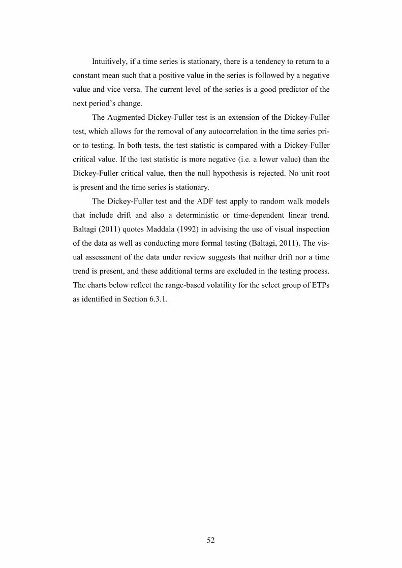
52

Intuitively, if a time series is stationary, there is a tendency to return to a

constant mean such that a positive value in the series is followed by a negative

value and vice versa. The current level of the series is a good predictor of the

next period’s change.

The Augmented Dickey-Fuller test is an extension of the Dickey-Fuller

test, which allows for the removal of any autocorrelation in the time series pri-

or to testing. In both tests, the test statistic is compared with a Dickey-Fuller

critical value. If the test statistic is more negative (i.e. a lower value) than the

Dickey-Fuller critical value, then the null hypothesis is rejected. No unit root

is present and the time series is stationary.

The Dickey-Fuller test and the ADF test apply to random walk models

that include drift and also a deterministic or time-dependent linear trend.

Baltagi (2011) quotes Maddala (1992) in advising the use of visual inspection

of the data as well as conducting more formal testing (Baltagi, 2011). The vis-

ual assessment of the data under review suggests that neither drift nor a time

trend is present, and these additional terms are excluded in the testing process.

The charts below reflect the range-based volatility for the select group of ETPs

as identified in Section 6.3.1.

53

Figure 5: Range-based Volatility for Select ETPs - Jan 2006 to July 2014 - Aggregated Data

United States: IVV Japan: EWJ Germany: EWG

South Korea: EWY Taiwan: EWT

.00

.04

.08

.12

.16

.20

2006 2007 2008 2009 2010 2011 2012 2013 2014

IVV

.00

.01

.02

.03

.04

.05

.06

.07

.08

.09

2006 2007 2008 2009 2010 2011 2012 2013 2014

EWJ

.00

.10

.20

.30

.40

.50

.60

.70

.80

2006 2007 2008 2009 2010 2011 2012 2013 2014

EWG

.00

.10

.20

.30

.40

.50

2006 2007 2008 2009 2010 2011 2012 2013 2014

EWY

.00

.05

.10

.15

.20

.25

.30

.35

2006 2007 2008 2009 2010 2011 2012 2013 2014

EWT

54

6.4.4.1.1 Dickey-Fuller Test

If we have an AR(1) model as below:

Equation 10

∆𝑦𝑡 = 𝛿𝑦𝑡−1 + 휀𝑡


𝑌0 = 0 𝑎𝑛𝑑 휀𝑡 = 𝑖𝑖𝑑[0, 𝜎2]

We are unable to make use of the Central Limit Theorem 3 and

conventional t-test statistics in testing for values of δ in the event that yt and yt-

1 are non-stationary. Instead, we make use of the Dickey-Fuller asymptotic

distribution to compare the t-statistic with a Dickey-Fuller critical value. The

testing hypothesis is given as:

H0: δ = 1 (unit root, non-stationary)

H1: δ < 1 (stationary)

If we accept the null hypothesis with δ = 1, this results in an AR(1) process

with a unit root and one which is non-stationary. We would visually observe

trends in the data over time.

6.4.4.1.2 Augmented Dickey-Fuller Test

For a process that is more complex than an AR(1) model, an AR(n) pro-

cess can be given with the form:

Equation 11

∆𝑦𝑡 = 𝛿𝑦𝑡−1 + ∑ 𝛽𝑖

ℎ

𝑖=1

∆𝑦𝑡−𝑖 + 휀𝑡


𝑌0 = 0 𝑎𝑛𝑑 휀𝑡 = 𝑖𝑖𝑑[0, 𝜎2]

Again, the testing hypothesis is given as:

H0: δ = 1 (unit root, non-stationary) 3 The sampling distribution of a statistic will follow a normal distribution, as long as

the sample size is sufficiently large

55

H1: δ < 1 (stationary)

If we accept the null hypothesis with δ = 1 results in an AR(n) process with a

unit root and one which is non-stationary. If we reject the null hypothesis, we

find δ < 1 and can conclude our time series is stationary.

6.4.4.1.2.1 Determination of Lags

In dealing with a more complex AR(n) process, we need to determine

how many lags – the number of 𝛽𝑖∆𝑦𝑡−𝑖 terms – we include in our specifica-

tion and testing. We add these lagged terms in order to correct for the presence

of serial correlation in the error terms. Even if the null hypothesis is true, in

other words we have a non-stationary series, we find that the estimators for the

β terms have a t-distribution which allows us to test the significance of the β

terms using t-tests or F-tests. If we add lag terms and find they are not signifi-

cant, then they should not be included in the specification. In this way, the

testing is a manually, iterative process to determine the correct number of lags

to specify.

Another way in which to determine the number the number of lags is to

continue adding them until the point at which we have no serial correlation in

the error term εt.

The selection of lag length is an important practical issue. If the number

of lags selected is too small, the remaining serial correlation in the errors will

bias the test. If the lag length selected it too large, the power of the test will

suffer. It is suggested that the inclusion of too many lags is the more “desira-

ble” error to make. A paper by Ng and Perron (1995) suggests conducting an

ADF test with a maximum number of lags. The absolute value of the t-statistic

for the last lag is examined. If that value is greater than 1.6, then the maximum

number of lags is determined. If the value is less than 1.6, the number of lags

should be reduced by 1 and the process conducted again (Ng & Perron, 1995).

This iterative testing method will be applied to the data under review to

determine the appropriate number of lags for the ADF test.

56

6.4.4.2 Phillips-Perron Unit Root Test

The Phillips-Perron Unit Root test is an alternative test to the ADF test

in determining the whether a time series is stationary or not. Considering a

stochastic time series model with the following form:

Equation 12

𝑌𝑡 = 𝜌𝑌𝑡−1 + 휀𝑡


𝑡 = 1, 2, … 𝑛

𝑌0 = 0 𝑎𝑛𝑑 휀𝑡 = 𝑖𝑖𝑑[0, 𝜎2]

The Phillips-Perron test makes use of a corrective form of the t-test to

determine a value for ρ. This corrective form of the test corrects for the poten-

tial of serial correlation and heteroscedasticity in the error terms. Importantly,

this corrective form of the test is non-parametric. Like the ADF test, the hy-

pothesis is:

H0: ρ = 1 (unit root, non-stationary)

H1: ρ < 1 (stationary)

The Phillips-Perron test does not require the specification of the number

of lags in the same way the ADF requires lag specification. This lack of lag

specification requirement is because the corrective form of the t-test is robust

to the presence of serial correlation and heteroskedasticity in the error terms. A

comparison of the test statistic with a Phillips-Perron critical value is

undertaken. If the test statistic is more negative (i.e. a lower value) than the

Phillips-Perron critical value, then the null hypothesis is rejected. No unit root

is present and the time series is stationary.

In work conducted in 2004, Davidson and MacKinnon determined that

for small, finite samples, the ADF test outperformed the Phillips-Perron test.

This finding, that it is best suited to large data samples, is the primary disad-

vantage of the Phillips-Perron test. However, given the dataset under review

contains 40 to 50 thousand data points for each ETP instrument, the results of

the Phillips-Perron test are unlikely to be affected by the problems addressed

57

by Davidson and MacKinnon (2004). In the interests of good practise to con-

duct multiple tests using varying approaches, the results of the Augmented

Dickey-Fuller test and the Phillips-Perron test are discussed in 6.4.4.3 below.

6.4.4.3 Results of Testing for Nonstationarity

The Augmented Dickey-Fuller test and the Phillips-Perron test were

conducted on the full date range of ETP range-based volatility. For each ETP,

the range-based volatility measure for each 15-minute sample within the trad-

ing day was included in the data set. Data from the 6 May 2010, Flash Crash

event, were excluded.

The ADF test results are presented in Appendix Section B.1. An analysis

of the test statistics generated by the Augmented Dickey-Fuller test shows that

for all ETP instruments, the test statistic was less negative (i.e. a higher value)

than the ADF critical value. For all ETPs, we accept the null hypothesis that

states that the series has a unit root and is non-stationary.

The choice of lag length for each ADF test pertaining to the various

ETPs is also presented in the results. The methodology outlined in Section

6.4.4.1.2.1 is applied to the lag length selection process. The appropriate num-

ber of lags range from 17 for the ETP with ticker EWU to a lag length of 24

for a number of ETPs.

An analysis of the test statistics of the Phillips-Perron Test presents con-

flicting results for all but one ETP instrument. For the ETP with ticker EWQ,

which is the iShares International ETP tracking the MSCI France index, the

test statistic is greater than the Phillips-Perron critical value. This allows for

the acceptance of the null hypothesis. The time series for EWQ has a unit root

and is non-stationary. No discernible differences between the distributions

characteristics of EWQ relative to the other ETP instruments under review can

be readily identified. Further, more extensive examination is required to ac-

count for this result. For all other ETPs instruments tested, the test statistics

are less than the Phillips-Perron critical values. We, therefore, reject the null

hypothesis and conclude that no unit root is present and the time series are sta-

tionary.

58

6.4.4.3.1 Addressing the Conflicting Results

While somewhat dissatisfying to achieve conflicting results from the

Augmented Dickey-Fuller test and the Phillips-Perron test, it is not unusual

when analysing financial time series data. Kwiatkowski, et al. (1992) state that

it is well-established that standard root tests fail to reject the null hypothesis

for many economic time series. The conclusion that is typically asserted from

an empirical analysis is that many economic time series contain a unit root.

Kwiatkowski, et al. (1992) explain that in tests such as the Augmented Dick-

ey-Fuller test and the Phillips-Perron test, the unit root is the null hypothesis

being tested. Given the way in which classical hypothesis testing is conducted

ensures the null hypothesis is accepted unless there is strong evidence against

it (Kwiatkowski, et al., 1992). They suggest further that it is therefore useful to

test the null hypothesis of stationarity as well as testing the null hypothesis of

a unit root. To provide support for either the findings of the Augmented Dick-

ey-Fuller test or the Phillips-Perron test, we introduce a third test of stationari-

ty, the Kwiatkowski-Phillips-Schmidt-Shin test, hereafter referred to as the

KPSS test.

6.4.4.4 The KPSS Test

The KPSS test is a stationary test – essentially opposite in hypothesis

structure to the ADF and Phillips-Perron tests. Starting with the model specifi-

cation below:

Equation 13

𝑦𝑡 = 𝛽′𝑫𝑡 + 𝜇𝑡 + 𝑢𝑡


𝜇𝑡 = 𝜇𝑡−1 + 휀𝑡, 휀𝑡~𝑊𝑁(0, 𝜎𝜀2)

Where 𝑫𝑡 contains a constant, or a constant and a time trend and

where 𝑢𝑡 = 𝐼(0). The hypothesis is given as:

H0: 𝜎𝜀2 = 0 (stationary)

H1: 𝜎𝜀2 > 0 (non-stationary)

59

The KPSS test is a one-sided, right-tailed test. The null of stationarity is

rejected at the 100∙α% level if the KPSS test statistic is greater than the 100∙(1-

α)% quantile from the appropriate asymptotic distribution (Zivot, 2006).

The results of the KPSS test are presented in the Appendix Section B.3

and serve to support the findings of the Augmented Dickey-Fuller test, which

accepted the null hypothesis of non-Stationarity of the range-based volatility

measure for all ETP instruments. The KPSS test statistics are greater than the

KPSS critical values, and we reject the null hypothesis of stationarity.

6.4.5 Conclusions from Stationarity Testing As is often the case when conducting empirical analysis, and particularly

when working with econometric or financial data series, the application of

formal statistical testing can be a complex process. The results of the Phillips-

Perron test conflict with the results obtained from the ADF test and the KPSS

test. Schwert (1989) finds that if ∆𝑦𝑡can be described by an ARMA process

and when that process contains a large and negative moving average compo-

nent, then both the ADF test and the Phillips-Perron test may provide errone-

ous results. These errors would present as a rejection of the unit root null hy-

pothesis too often when it is true. This is particularly true of the Phillips-

Perron test (Schwert, 1989). Caner and Killian (2001) suggest that the KPSS

test suffers from similar problems to the ADF and Phillips-Perron tests.

If we consider the data under review and make some intuitive comments,

we should be unsurprised that the data appears to be non-stationary. During

the period January 2006 to July 2014, financial markets experienced a major

market and economic crisis. The Great Recession catalysed by the 2007/08

Credit Crisis undoubtedly resulted in a volatility profile which was different to

the periods before and after the crisis. In order to determine whether this peri-

od in financial market history was accountable for the findings of non-

stationarity, some preliminary testing was conducted. The ETP subset as iden-

tified in Section 6.3.1 was testing over a truncated date range to exclude the

period from January 2007 to December 2008. The ADF test, Phillips-Perron

test and KPSS test were conducted.

60

The results from this preliminary testing were mixed and inconclusive

regarding the stationarity of the data series excluding the crisis period. Given

the result ambiguity, and the desire to use a non-truncated dataset, the full date

range from January 2006 to July 2014, excluding the Flash Crash event, will

be used for additional analysis work.

6.5 Preparation for Statistical Analysis

We are attempting to determine whether those ETPs with underlying

baskets that are listed in non-synchronous or partially synchronous markets to

the ETP instrument exhibit a different volatility profile to ETPs with

underlying baskets listed in synchronous markets to the ETP instrument itself.

The volatility profile is measured by range-based volatility. We are now in a

position to make informed choices on the statistical tests we will apply to

evaluate and interpret the data.

Given our initial visual data analysis we exclude the data computed for 6

May 2010 in order to exclude the Flash Crash event. Although non-US baskets

were less affected by the Flash Crash event, to ensure a consistent approach

that date point is removed from all range-based volatility datasets.

The initial statistical analysis indicated two critical features of the data,

namely:

1. The data are not normally distributed

2. The data are not stationary

The first feature can be addressed by ensuring that any statistical tests

can provide accurate results for a non-normal dataset. Catering for non-normal

data implies a selection of non-parametric testing processes. For the second

feature, to make allowance for the non-stationarity of the data we must ensure

that the statistical methods selected are not invalidated by this finding.

61

6.5.1 Non-Parametric Tests Non-parametric tests are appropriate when no assumptions (i.e. normali-

ty) can be made about the underlying distribution of the data. Non-parametric

tests are typically more robust than the equivalent parametric test, but non-

parametric tests tend to have less statistical power and can often be more diffi-

cult to interpret.

The objective of this analysis is to determine whether there is a

difference in volatility profile between non-synchronous, partially

synchronous and synchronous ETPs. A statistical test is required that allows

for the comparison of the median value of the range-based volatility measure

of those ETPs with foreign underlying baskets, to the median value of the

range-based volatility measure of the ETP which contains domestic, NYSE-

listed securities as its underlying basket. Practically, that means comparing the

median of each range-based volatility measure for ETP during every 15-

minute time interval to the range-based volatility of the United States ETP

with ticker IVV.

The two statistical tests typically used to compare the medians when the

data are non-parametric are the Mann-Whitney U test and the Wilcoxon

Signed Rank test.

6.5.1.1 Mann-Whitney U Test

The Mann-Whitney U test is a rank-based non-parametric test that can

be used to determine if there are differences between two groups, either

differences in the distributions of the two groups or differences in the medians

of the two groups. It is often presented as an alternative to the t-test when

normality assumptions fail or when the data are ordinal. To use the Mann-

Whitney U test to determine whether there is a difference in medians between

two groups, we need to need to meet the assumption that the distribution of the

two groups is the same. The following general assumptions also need to be

met:

62

1. One independent variable measured at the continuous or ordinal

level.

2. One independent variable consisting of two categorical,

independent groups.

3. Independence of observations – there is no relationship between

the observations. (Laerd Statistics, n.d.)

Intuitively, the third general assumption is concerning given the finan-

cial data under review. Stock markets do not move independently of one

another, and economic, geopolitical or other material sentiment drivers affect

global markets. Yunus (2013) studied the dynamic interdependence between

ten major markets over the period 1993 to 2008 using a recursive cointegration

technique. Results indicated that international financial markets are integrated

and bound together by four long-run relationships. The results also revealed

that the United States contributes the most heavily to the common trends. This

indicates the pre-eminent position of the United States as the global leader in

that it leads and drives each of the other markets (Yunus, 2013).

As such, the likely violation of the third general assumption of the

Mann-Whitney U indicates that the test is inappropriate for the purposes of

this analysis.

6.5.1.2 Wilcoxon Signed Rank Test

The Wilcoxon Signed Rank test is a nonparametric test equivalent to the

dependent t-test that does not rely on a normally distributed underlying da-

taset. It is typically used to compare two sets of results that come from the

same dataset and carries the following general assumptions which need to be

met in order to ensure statistical validity:

1. An independent variable that is measured at the continuous or

ordinal level.

2. The independent variable should consist of two categorical, "re-

lated groups" or "matched pairs". “Related groups” typically

63

means the same subjects are present in both groups while

“matched pairs” refers to different subjects.

3. The distribution of the differences between the two related

groups needs to be symmetrical in shape.

Provided the range-based volatility data under review is able to satisfy

the third required general assumption, the Wilcoxon Signed Rank test will

provide an appropriate measure for answering the research question.

6.6 Statistical Analysis

6.6.1 Initial Statistical Analysis The objective of the statistical analysis is to compare the median value

of each ETP’s range-based volatility measure in each 15-minute data interval

to the median value of the ETP holding an underlying basket of stocks all

listed in the United States. By comparing the medians of the non-synchronous,

partially synchronous and synchronous ETP’s with that of the ETP tracking a

basket of United States equities, we can begin to understand whether there is

any persistence in range-based volatility characteristics of the ETP’s whose

underlying baskets are in different time zones to the time zone of the instru-

ment listing.

As a mechanism of the initial analysis, the charts below display range-

based volatility measure for each ETP for each 15-minute intra-day time inter-

val graphically displayed as a box plot. For the sake of clarity, we are compar-

ing the median value of every ETP to the median value of the ETP with ticker

IVV – the ETP tracking an underlying basket of Unites States equities.

We therefore have 26 box plots reflecting the 26, 15-minute intraday in-

tervals through the trading day. Note that the range-based volatility measure is

determined from the open, high, low, close intraday price data over the time

period the 1 January 2006 to the 11 July 2014. The data from the 6 May 2010

are excluded to remove the extreme effect of the Flash Crash.

64

Figure 6: Box Plot for All ETPs for Each 15-minute Intraday Interval

9.30am EST 9.45am EST 10.00am EST



.000

.001

.002

.003

.004

.005

.006

.007

.008

EWA1

EWC1

EWD1

EWG1

EWH1

EWI1

EWJ1

EWK1

EWL1

EWM1

EWN1

EWO1

EWP1

EWQ1

EWS1

EWT1

EWU1

EWW

1EW

Y1EW

Z1IV

V1.0000

.0005

.0010

.0015

.0020

.0025

.0030

.0035

EWA2

EWC2

EWD2

EWG2

EWH2

EWI2

EWJ2

EWK2

EWL2

EWM2

EWN2

EWO2

EWP2

EWQ2

EWS2

EWT2

EWU3

EWW

2EW

Y2EW

Z2IV

V2.0000

.0005

.0010

.0015

.0020

.0025

.0030

.0035

.0040

EWA3

EWC3

EWD3

EWG3

EWH3

EWI3

EWJ3

EWK3

EWL3

EWM3

EWN3

EWO3

EWP3

EWQ3

EWS3

EWT3

EWU3

EWW

3EW

Y3EW

Z3IV

V3

.0000

.0005

.0010

.0015

.0020

.0025

.0030

EWA4

EWC4

EWD4

EWG4

EWH4

EWI4

EWJ4

EWK4

EWL4

EWM4

EWN4

EWO4

EWP4

EWQ4

EWS4

EWT4

EWU4

EWW

4EW

Y4EW

Z4IV

V4.0000

.0004

.0008

.0012

.0016

.0020

.0024

EWA5

EWC5

EWD5

EWG5

EWH5

EWI5

EWJ5

EWK5

EWL5

EWM5

EWN5

EWO5

EWP5

EWQ5

EWS5

EWT5

EWU5

EWW

5EW

Y5EW

Z5IV

V5.0000

.0004

.0008

.0012

.0016

.0020

EWA6

EWC6

EWD6

EWG6

EWH6

EWI6

EWJ6

EWK6

EWL6

EWM6

EWN6

EWO6

EWP6

EWQ6

EWS6

EWT6

EWU6

EWW

6EW

Y6EW

Z6IV

V6

.0000

.0004

.0008

.0012

.0016

.0020

EWA7

EWC7

EWD7

EWG7

EWH7

EWI7

EWJ7

EWK7

EWL7

EWM7

EWN7

EWO7

EWP7

EWQ7

EWS7

EWT7

EWU7

EWW

7EW

Y7EW

Z7IV

V7.0000

.0004

.0008

.0012

.0016

.0020

EWA8

EWC8

EWD8

EWG8

EWH8

EWI8

EWJ8

EWK8

EWL8

EWM8

EWN8

EWO8

EWP8

EWQ8

EWS8

EWT8

EWU8

EWW

8EW

Y8EW

Z8IV

V8.0000

.0002

.0004

.0006

.0008

.0010

.0012

.0014

EWA9

EWC9

EWD9

EWG9

EWH9

EWI9

EWJ9

EWK9

EWL9

EWM9

EWN9

EWO9

EWP9

EWQ9

EWS9

EWT9

EWU9

EWW

9EW

Y9EW

Z9IV

V9

65

11.45am EST 12.00 pm EST 12.15pm EST

12.30pm EST 12.45pm EST 1.00pm EST


.0000

.0002

.0004

.0006

.0008

.0010

.0012

.0014

EWA10

EWC10

EWD10

EWG10

EWH10

EWI10

EWJ10

EWK10

EWL10

EWM10

EWN10

EWO10

EWP10

EWQ10

EWS10

EWT10

EWU10

EWW

10

EWY10

EWZ10

IVV10

.0000

.0002

.0004

.0006

.0008

.0010

.0012

EWA11

EWC11

EWD11

EWG11

EWH11

EWI11

EWJ11

EWK11

EWL11

EWM11

EWN11

EWO11

EWP11

EWQ11

EWS11

EWT11

EWU11

EWW

11

EWY11

EWZ11

IVV11

.0000

.0002

.0004

.0006

.0008

.0010

.0012

EWA12

EWC12

EWD12

EWG12

EWH12

EWI12

EWJ12

EWK12

EWL12

EWM12

EWN12

EWO12

EWP12

EWQ12

EWS12

EWT12

EWU12

EWW

12

EWY12

EWZ12

IVV12

.0000

.0002

.0004

.0006

.0008

.0010

.0012

EWA13

EWC13

EWD13

EWG13

EWH13

EWI13

EWJ13

EWK13

EWL13

EWM13

EWN13

EWO13

EWP13

EWQ13

EWS13

EWT13

EWU13

EWW

13

EWY13

EWZ13

IVV13

.0000

.0002

.0004

.0006

.0008

.0010

EWA14

EWC14

EWD14

EWG14

EWH14

EWI14

EWJ14

EWK14

EWL14

EWM14

EWN14

EWO14

EWP14

EWQ14

EWS14

EWT14

EWU14

EWW

14

EWY14

EWZ14

IVV14

.0000

.0002

.0004

.0006

.0008

.0010

.0012

EWA15

EWC15

EWD15

EWG15

EWH15

EWI15

EWJ15

EWK15

EWL15

EWM15

EWN15

EWO15

EWP15

EWQ15

EWS15

EWT15

EWU15

EWW

15

EWY15

EWZ15

IVV15

.0000

.0002

.0004

.0006

.0008

.0010

.0012

EWA16

EWC16

EWD16

EWG16

EWH16

EWI16

EWJ16

EWK16

EWL16

EWM16

EWN16

EWO16

EWP16

EWQ16

EWS16

EWT16

EWU16

EWW

16

EWY16

EWZ16

IVV16

.0000

.0002

.0004

.0006

.0008

.0010

.0012

EWA17

EWC17

EWD17

EWG17

EWH17

EWI17

EWJ17

EWK17

EWL17

EWM17

EWN17

EWO17

EWP17

EWQ17

EWS17

EWT17

EWU17

EWW

17

EWY17

EWZ17

IVV17

.0000

.0002

.0004

.0006

.0008

.0010

.0012

EWA18

EWC18

EWD18

EWG18

EWH18

EWI18

EWJ18

EWK18

EWL18

EWM18

EWN18

EWO18

EWP18

EWQ18

EWS18

EWT18

EWU18

EWW

18

EWY18

EWZ18

IVV18

66



3.30pm EST 3.45pm EST

.0000

.0002

.0004

.0006

.0008

.0010

.0012

.0014

EWA19

EWC19

EWD19

EWG19

EWH19

EWI19

EWJ19

EWK19

EWL19

EWM19

EWN19

EWO19

EWP19

EWQ19

EWS19

EWT19

EWU19

EWW

19

EWY19

EWZ19

IVV19

.0000

.0002

.0004

.0006

.0008

.0010

.0012

.0014

.0016

EWA20

EWC20

EWD20

EWG20

EWH20

EWI20

EWJ20

EWK20

EWL20

EWM20

EWN20

EWO20

EWP20

EWQ20

EWS20

EWT20

EWU20

EWW

20

EWY20

EWZ20

IVV20

.0000

.0002

.0004

.0006

.0008

.0010

.0012

.0014

EWA21

EWC21

EWD21

EWG21

EWH21

EWI21

EWJ21

EWK21

EWL21

EWM21

EWN21

EWO21

EWP21

EWQ21

EWS21

EWT21

EWU21

EWW

21

EWY21

EWZ21

IVV21

.0000

.0002

.0004

.0006

.0008

.0010

.0012

.0014

EWA22

EWC22

EWD22

EWG22

EWH22

EWI22

EWJ22

EWK22

EWL22

EWM22

EWN22

EWO22

EWP22

EWQ22

EWS22

EWT22

EWU22

EWW

22

EWY22

EWZ22

IVV22

.0000

.0002

.0004

.0006

.0008

.0010

.0012

.0014

.0016

EWA23

EWC23

EWD23

EWG23

EWH23

EWI23

EWJ23

EWK23

EWL23

EWM23

EWN23

EWO23

EWP23

EWQ23

EWS23

EWT23

EWU23

EWW

23

EWY23

EWZ23

IVV23

.0000

.0002

.0004

.0006

.0008

.0010

.0012

.0014

EWA24

EWC24

EWD24

EWG24

EWH24

EWI24

EWJ24

EWK24

EWL24

EWM24

EWN24

EWO24

EWP24

EWQ24

EWS24

EWT24

EWU24

EWW

24

EWY24

EWZ24

IVV24

.0000

.0002

.0004

.0006

.0008

.0010

.0012

.0014

.0016

EWA25

EWC25

EWD25

EWG25

EWH25

EWI25

EWJ25

EWK25

EWL25

EWM25

EWN25

EWO25

EWP25

EWQ25

EWS25

EWT25

EWU25

EWW

25

EWY25

EWZ25

IVV25

.0000

.0004

.0008

.0012

.0016

.0020

EWA26

EWC26

EWD26

EWG26

EWH26

EWI26

EWJ26

EWK26

EWL26

EWM26

EWN26

EWO26

EWP26

EWQ26

EWS26

EWT26

EWU26

EWW

26

EWY26

EWZ26

IVV26

67

6.6.1.1 Preliminary Results from the Wilcoxon Signed Rank Test

Upon commencement of the computations of statistics for the Wilcoxon

Signed Rank test, it became immediately evident that the third assumption of

the test which states that the distribution of differences between the two time

series needs to be symmetrical was violated. Voraprateep (2013) demonstrates

that when the distribution changes from symmetry to asymmetry, the power of

Wilcoxon signed-rank test decreases showing that the Wilcoxon signed-rank

test is not applicable to an asymmetric distribution (Voraprateep, 2013). Given

this violation, the available literature proposed two possible alternatives. The

first alternative was to make use instead of the Sign test as opposed to the Wil-

coxon Signed Rank test. The assumptions for the Sign test are provided below:

1. The dependent variable should be measured on a continuous (i.e.,

interval or ratio) or ordinal level.

2. The independent variable should consist of two categorical, "re-

lated groups" or "matched pairs".

3. The paired observations for each participant need to be inde-

pendent. That is, one participant's values cannot influence anoth-

er participant's values.

4. The difference scores (i.e., differences between the paired obser-

vations) are from a continuous distribution. (Laerd Statistics,

n.d.)

Assumption 3 has a requirement for independence and given the ra-

tionale for selecting the Wilcoxon Signed Rank test rather than the Mann-

Whitney U test, the Sign test will be inappropriate for the analysis of these da-

ta.

The second alternative is to transform the data in some way in order to

adhere to the conditions of symmetry. Suggested transformations include an

inverse or reciprocal transformation, taking the logarithm of the data (when

the data are non-negative), taking the square root and other power transfor-

mations. As the data under review are non-negative and given that taking the

natural logarithm of the data is a useful technique to reduce skewness in par-

68

ticular and therefore often used with financial data, the range-based volatility

for each ETP for each 15-minute intraday time interval will be transformed by

computing the natural logarithm. Under ideal conditions, the transformation of

the data by taking the natural logarithm would normalise the distribution to the

extent that parametric tests could be applied rather than non-parametric tests.

Unfortunately, despite the transformation, the data remain non-normally dis-

tributed and as such, the non-parametric Wilcoxon Signed Rank test will be

used.

6.6.1.2 Data Transformation and Test Specification

For each ETP as presented in the box plots above, the range-based

volatility measure for each 15-minute intraday interval, was transformed by

taking the natural logarithm of the range-based volatility measure. As the ob-

jective of this analysis is to determine whether there is a difference in volatility

profile between non-synchronous, partially synchronous and synchronous

ETPs, we compare the median value of the transformed range-based volatility

measure for each 15-minute time interval of each ETP with a foreign underly-

ing basket, to the median value of the transformed range-based volatility

measure for of the ETP listed on the NYSE which contains NYSE-listed secu-

rities as its underlying basket, the ETP with ticker symbol IVV.

We carry out a test of the null hypothesis that the median of transformed,

rang-based data of the foreign ETP is equal to the specified value of the medi-

an of the United States ETP against the two-sided alternative that it is not

equal to the median of the United States ETP - IVV:

H0: 𝑚𝑒𝑑(𝑥) = 𝑚

H1: 𝑚𝑒𝑑(𝑥) ≠ 𝑚


𝑚 = 𝑚𝑒𝑑𝑖𝑎𝑛 𝑣𝑎𝑙𝑢𝑒 𝑜𝑓 𝐼𝑉𝑉

The Eviews statistical software reports a p-value for the asymptotic

normal approximation to the Wilcoxon t-statistic (correcting for both continui-

ty and tied or numerically equal points). It is based on the premise of the Wil-

69

coxon Signed Rank test that if the absolute value of the difference between

each observation and the median ranked from high to low is summed, the sum

of the ranks above the median should be similar to the sum of the ranks below

the median (Eviews 8 Users Guide I, 2014). Eviews also reports the number of

observations above and below the specified median value as well as the mean

rank. This provides a useful indication as to whether the tested median is

above or below the specified median in the event that we reject the null hy-

pothesis of the Wilcoxon Signed Rank test and accept the alternative.

Full details of the results of the Wilcoxon Signed Rank test are provided

in the supporting documentation. A summary of the findings will be discussed

below.

6.6.2 Results of the Wilcoxon Signed Rank Test The results of the Wilcoxon Signed Rank test were unanimous and un-

ambiguous across all ETPs and for each 15-minute intraday period. No ETP

exhibited a median that was statistically equivalent to the median of the ETP

tracking the underlying basket of stocks listed in the United States with ticker

IVV. For all ETPs and for each intraday time interval, we reject the null hy-

pothesis of equal medians and accept the alternative hypothesis of non-equal

medians.

For each ETP and for each 15-minute intraday interval over the data

range, we are able to identify how many observations fall above the median of

the United State ETP and how many observations fall below the median of the

United States ETP. Given the total number of observations, we can determine

on a percentage basis, how many observation fall above the United States ETP

median and how many below. These observations were then plotted graphical-

ly and can be found below separated into non-synchronous, partially synchro-

nous and synchronous groups.

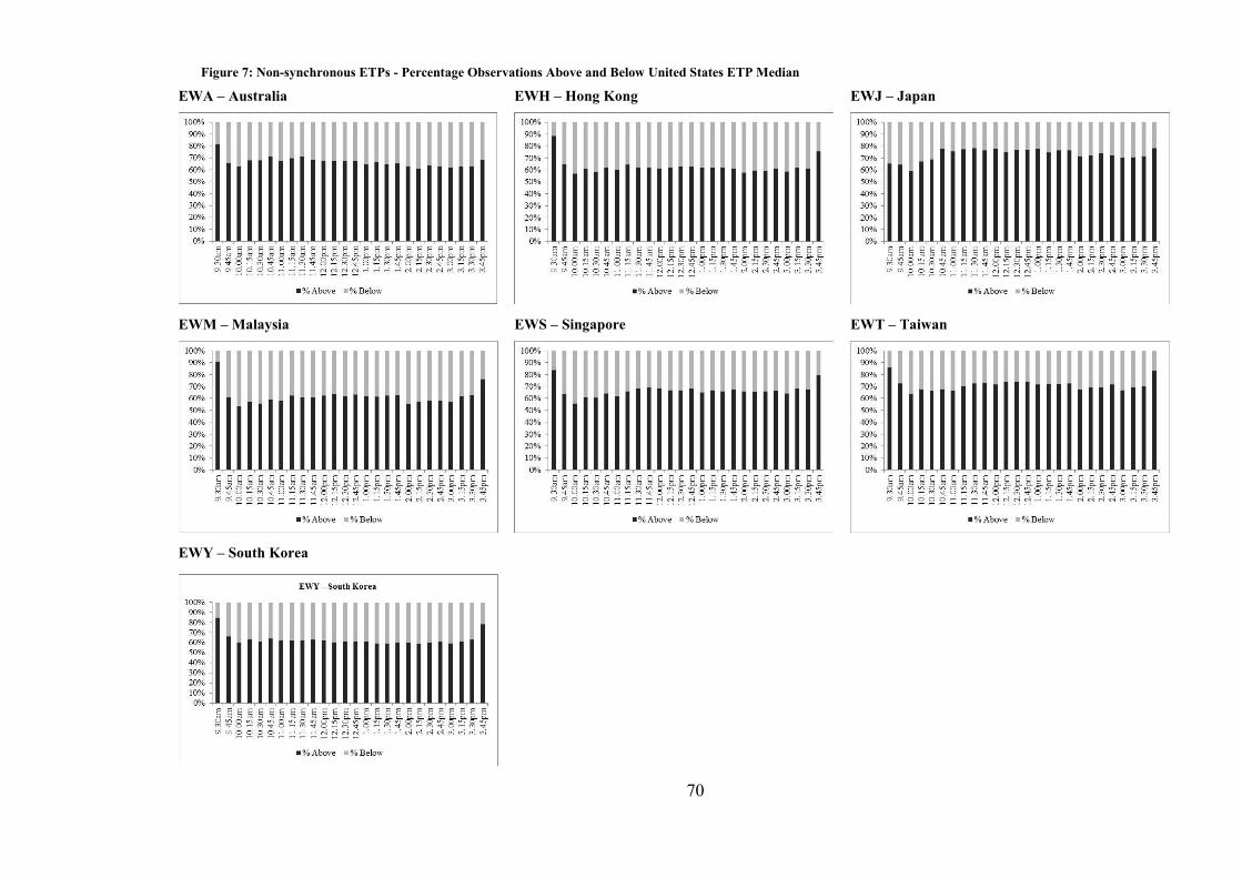
70

Figure 7: Non-synchronous ETPs - Percentage Observations Above and Below United States ETP Median

EWA – Australia EWH – Hong Kong EWJ – Japan

EWM – Malaysia EWS – Singapore EWT – Taiwan

EWY – South Korea

71

Figure 8: Partially synchronous ETPs - Percentage Observations Above and Below United States ETP Median

EWD – Sweden EWG – Germany EWI – Italy

EWK – Belgium EWL – Switzerland EWN – Netherlands

EWO – Austria EWP – Spain EWQ – France

72

EWU – United Kingdom

Figure 9: Synchronous ETPs - Percentage Observations Above and Below United States ETP Median

EWC – Canada EWW – Mexico EWZ – Brazil

73

6.6.2.1 Discussion of Wilcoxon Signed Rank Test Results

The graphical results provide some interesting qualitative insights and

suggest avenues for further interrogation and research. Additionally, an aver-

age is presented both for each ETP where the average for the individual ETPs

is given as:

Equation 14

𝐴𝑣𝑒 % 𝐴𝑏𝑜𝑣𝑒 𝐼𝑉𝑉 = ∑ 𝑃𝑝𝑜𝑠𝑖

𝑛𝑖=1

𝑛

Equation 15

𝐴𝑣𝑒 % 𝐵𝑒𝑙𝑜𝑤 𝐼𝑉𝑉 = ∑ 𝑃𝑛𝑒𝑔𝑖

𝑛𝑖=1

𝑛


𝑃𝑝𝑜𝑠𝑖 = % 𝑜𝑏𝑠𝑒𝑟𝑣𝑎𝑡𝑖𝑜𝑛𝑠 𝑎𝑏𝑜𝑣𝑒 𝐼𝑉𝑉 𝑚𝑒𝑑𝑖𝑎𝑛 𝑓𝑜𝑟 𝑡𝑖𝑚𝑒 𝑖𝑛𝑡𝑒𝑟𝑣𝑎𝑙 𝑖

𝑃𝑛𝑒𝑔𝑖 = % 𝑜𝑏𝑠𝑒𝑟𝑣𝑎𝑡𝑖𝑜𝑛𝑠 𝑏𝑒𝑙𝑜𝑤 𝐼𝑉𝑉 𝑚𝑒𝑑𝑖𝑎𝑛 𝑓𝑜𝑟 𝑡𝑖𝑚𝑒 𝑖𝑛𝑡𝑒𝑟𝑣𝑎𝑙 𝑖

𝑛 = 𝑛𝑢𝑚𝑏𝑒𝑟 𝑜𝑓 15 𝑚𝑖𝑛𝑢𝑡𝑒 𝑖𝑛𝑡𝑟𝑎𝑑𝑎𝑦 𝑖𝑛𝑡𝑒𝑟𝑣𝑎𝑙𝑠

In addition to computing a simple average for each individual ETP

across the 26 intraday, 15-minute time intervals, a simple average for the non-

synchronous, partially synchronous and synchronous groups is also presented.

These statistics form the basis of a qualitative or observational discussion pre-

sented below.

Table 4: Average Percentages Above and Below IVV Median per ETP

Ave % Above IVV

Median

Ave % Below IVV

Median

Non-Synchronous ETP

Group Average 66.35% 33.65%

EWA – Australia 66.60% 33.40%

EWH – Hong Kong 62.63% 37.37%

EWJ – Japan 73.19% 26.81%

EWM – Malaysia 61.57% 38.43%

EWS – Singapore 66.54% 33.46%

EWT – Taiwan 71.20% 28.80%

EWY – South Korea 62.69% 37.31%

74

Partially Synchronous ETP


EWD – Sweden 59.76% 40.24%

EWG – Germany 59.20% 40.80%

EWI – Italy 58.68% 41.32%

EWK – Belgium 51.06% 48.94%

EWL – Switzerland 46.60% 53.40%

EWN – Netherlands 41.67% 58.33%

EWO – Austria 53.08% 46.92%

EWP – Spain 59.52% 40.48%

EWQ – France 49.74% 50.26%

EWU – United Kingdom 60.06% 39.94%

Synchronous ETP


EWC – Canada 62.23% 37.77%

EWW – Mexico 76.43% 23.57%

EWZ – Brazil 91.99% 8.01%

6.6.2.1.1 Non-Synchronous ETP Group

The non-synchronous ETPs, in other words, those ETPs which have un-

derlying stock baskets that trade on exchanges with no overlapping market

hours with the New York Stock Exchange show levels of range-based volatili-

ty that are persistently higher than the equivalent range-based volatility meas-

ure for the United States ETP with ticker IVV. Examining the average per-

centages above and below the ETP median, we observe that Japan and Taiwan

tend to exhibit more observations above the IVV median than do the other

members of the non-synchronous group. The average for the group shows that

two-thirds of group observations are higher than the equivalent IVV median.

An examination of the associated graphical representation indicates that

the opening and closing 15-minutes of the New York trading day show levels

of range-based volatility for the non-synchronous group as being observation-

ally higher than the equivalent IVV measure 83% and 77% of the time respec-

tively.

6.6.2.2 Partially Synchronous ETP Group

The partially synchronous group offers some interesting observations. In

contrast to the non-synchronous group, the ETPs with underlying baskets rep-

75

resenting the markets of Switzerland, the Netherland and France, show their

percentage observations above the IVV median to be less than 50%. Observa-

tionally, this implies the range-based volatility of these ETPs tends to be less

than the equivalent range-based volatility measure of IVV. And, also in con-

trast to the non-synchronous group, only the ETP with a United Kingdom un-

derlying basket displays observations above the median of IVV 60% or more

of observations.

As a group, the partially synchronous ETPs display a tendency to have a

lower number of observations greater than or above the equivalent IVV obser-

vation relative to their non-synchronous counterparts.

Through a visual examination of the graphical output, it can be observed

that apart from the first 15-minute time interval of the New York trading day

when as a group, 68% of observations are above the equivalent IVV median,

the time intervals from 11:15am to 11:30am and from 11:30am to 11:45am

show a higher percentage of observation above the IVV median than any other

15-minute intraday interval with percentage observations above the median

ranging between 62% and 66% respectively. The closing 15-minute interval

for the group shows 58% of observations above the IVV equivalent.

Upon review the information contained in Figure 2, we note that the Ital-

ian market closes first at 11:25am, followed by France, Spain, Switzerland,

Sweden and the United Kingdom at 11:30am, Austria at 11:35am and Belgium

and the Netherlands at 11:40am. The German market is unique as it remains

open for trading through to the New York market close at 4:00pm.

Intuitively, it appears from these observations that the close of the par-

tially synchronous markets midway through the trading day is impacting on

the range-based volatility measure of these ETPs. It is an area for further in-

vestigation and analysis.

6.6.2.3 Synchronous ETP Group

The Synchronous ETP group also offers interesting observations. A log-

ical assumption might be that as the underlying markets are open during the

New York trading day, there could be more certainty in the establishment and

76

verification of the ETP NAV – the valuation of the underlying basket – lead-

ing to less uncertainty in the pricing of the ETP instrument and hence a lower

measure of range-based volatility. Under these circumstances, we could expect

the median levels of Canadian, Mexican and Brazilian ETPs to show a closer

alignment to the median levels of the United States ETP. The findings are,

however, contrary to this assumption.

All three synchronous ETPs show a higher percentage of observations

above the IVV median value and the ETP tracking an underlying basket of

Brazilian stocks exhibits the highest percentage observations above the IVV

median with a value of 92%.

There would appear to be another factor at work driving the range-based

volatility measures. The obvious candidate for this disparity is currency influ-

ences. While the ETP instruments themselves are listed on the New York

Stock Exchange and priced in United States Dollars, the underlying basket of

stocks are priced in their respective local currencies and then translated into

United States Dollars at the prevailing exchange rate to establish a US Dollar

based Net Asset Value.

6.6.2.4 Additional Areas of Investigation

Following on from the results and qualitative interpretation above, two

findings will be investigated more thoroughly. The first is an analysis of the

apparent effect on the range-based volatility of the partially synchronous

group during the intervals which encompass the closing of their respective un-

derlying markets.

The second area of investigation will be an analysis of the role that for-

eign exchange plays in the results obtained.

77

Chapter 7

7 Partially Synchronous ETPs

7.1 European Market Closing

As discussed in 6.6.2.2, the closing of the partially synchronous or Eu-

ropean markets mid-morning during the United States trading day appears to

have some effect on the range-based volatility measure of those ETPs with

European underlying baskets. This perceived effect will be tested more close-

ly.

Again, making use of the Wilcoxon Signed Rank Test as outlined in

6.5.1.2, an analysis of the median value of the range-based volatility measure

of each partially synchronous ETP will be tested in two ways. As observed in

6.6.2.2, the time intervals from 11:15am to 11:30am and from 11:30am to

11:45am show a higher percentage of observations above the IVV median.

Instead of comparing the median value of the foreign ETP to the median value

of the United States ETP, the median value for each foreign ETP in the 15-

minute time interval from 11:00am to 11:15am will firstly be compared to the

median value for that same ETP in the 15-minute time interval from 11:15am

to 11:30am. Secondly, the median value in the 15-minute time interval from

11:30am to 11:45am will be compared to the median value of the same ETP in

the 15-minute time interval from 11:45am to 12:00pm. By conducting and

assessing the results of these two tests, some insight will be gained into

whether the range-based volatility is different during the European market

closing interval than in the 15-minute intervals immediately preceding and fol-

lowing the close.

Again, in order to comply with the assumptions of the Wilcoxon Signed

Rank Test, transformed data will be used, where the natural logarithm of the

78

range-based volatility measure will be tested rather than the underlying range-

based volatility measure itself.

The Wilcoxon Signed Rank Tests are specified as follows:




𝑚 = 𝑚𝑒𝑑𝑖𝑎𝑛 𝑣𝑎𝑙𝑢𝑒 𝑜𝑓 𝑖𝑛𝑡𝑒𝑟𝑣𝑎𝑙 11: 00𝑎𝑚 𝑡𝑜 11: 15𝑎𝑚




𝑚 = 𝑚𝑒𝑑𝑖𝑎𝑛 𝑣𝑎𝑙𝑢𝑒 𝑜𝑓 𝑖𝑛𝑡𝑒𝑟𝑣𝑎𝑙 11: 45𝑎𝑚 𝑡𝑜 12: 00𝑝𝑚

7.1.1 Results of the Wilcoxon Signed Rank Test – Partially

synchronous ETPs The test statistics are presented in full in Appendix C, but are discussed

below. In comparing the median value of each ETP in the time interval

11:00am to 11:15am to the median value of that same ETP in the time interval

from 11:15am to 11:30am, we find that for three of the ETPs, we can accept

the null hypothesis of equal medians.

For the ETP with ticker EWU tracking the United Kingdom underlying

stock basket, the ETP with ticker EWO tracking the Austrian underlying stock

basket and for the ETP with ticker EWK tracking the Belgium underlying

stock basket, we find Wilcoxon Signed Rank test statistics of 0.199 (p-value =

0.84) and 2.48 (p-value = 0.013) and 1.08 (p-value = 0.28) respectively. The

median values are not statistically different in the first 15-minute time interval

to the second 15-minute time interval for these three ETPs. For the remaining

ETPs in the partially synchronous basket, we reject the null hypothesis and

find that the median values in the first 15-minute time interval are different to

the median values in the second 15-minute time interval.

In comparing the median value of each ETP in the time interval 11:30am

to 11:45am to the median value of that same ETP in the time interval from

79

11:45am to 12:00pm, we find that for all of the ETPs in the partially synchro-

nous basket, we reject the null hypothesis. The median values in the time peri-

od 11:30am to 11:45am are statistically different to the median values in the

time period 11:45am to 12:00pm.

Again, the Wilcoxon Signed Rank test statistic does not provide an indi-

cation of the direction or magnitude of the difference in median values, and so

for the purposes of qualitative discussion, the percentage observations above

and below the median are presented.


11:15am Compared with Median in Interval 11:15am to 11:30am for Partially Synchronous ETPs

% Above

Median

% Below

Median

EWD – Sweden 46.53% 52.84%

EWG – Germany 48.56% 51.14%

EWI – Italy 45.38% 54.08%

EWK – Belgium 47.10% 53.14%



EWO – Austria 46.73% 53.31%

EWP – Spain 46.60% 52.79%

EWQ – France 45.26% 53.69%



11:45am Compared with Median in Interval 11:45am to 12:00pm for Partially Synchronous ETPs

% Above

Median

% Below

Median

EWD – Sweden 49.84% 50.28%

EWG – Germany 54.33% 42.90%

EWI – Italy 50.99% 48.44%

EWK – Belgium 50.80% 48.98%



EWO – Austria 50.56% 49.15%

EWP – Spain 52.71% 44.43%

EWQ – France 52.03% 46.16%


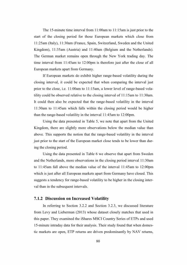
80

The 15-minute time interval from 11:00am to 11:15am is just prior to the

start of the closing period for those European markets which close from

11:25am (Italy), 11:30am (France, Spain, Switzerland, Sweden and the United

Kingdom), 11:35am (Austria) and 11:40am (Belgium and the Netherlands).

The German market remains open through the New York trading day. The

time interval from 11:45am to 12:00pm is therefore just after the close of all

European markets apart from Germany.

If European markets do exhibit higher range-based volatility during the

closing interval, it could be expected that when comparing the interval just

prior to the close, i.e. 11:00am to 11:15am, a lower level of range-based vola-

tility could be observed relative to the closing interval of 11:15am to 11:30am.

It could then also be expected that the range-based volatility in the interval

11:30am to 11:45am which falls within the closing period would be higher

than the range-based volatility in the interval 11:45am to 12:00pm.

Using the data presented in Table 5, we note that apart from the United

Kingdom, there are slightly more observations below the median value than

above. This supports the notion that the range-based volatility in the interval

just prior to the start of the European market close tends to be lower than dur-

ing the closing period.

Using the data presented in Table 6 we observe that apart from Sweden

and the Netherlands, more observations in the closing period interval 11:30am

to 11:45am fall above the median value of the interval 11:45am to 12:00pm

which is just after all European markets apart from Germany have closed. This

suggests a tendency for range-based volatility to be higher in the closing inter-

val than in the subsequent intervals.

7.1.2 Discussion on Increased Volatility In referring to Section 3.2.2 and Section 3.2.3, we discussed literature

from Levy and Lieberman (2013) whose dataset closely matches that used in

this paper. They examined the iShares MSCI Country Series of ETPs and used

15-minute intraday data for their analysis. Their study found that when domes-

tic markets are open, ETP returns are driven predominantly by NAV returns,

81

in other words, the pricing of the underlying securities listed on the domestic

market. They then found that when the underlying domestic market closed, the

ETP returns were dominated by the returns of the S&P 500. They determined

that there was a “regime shift” which occurred for European ETPs with the

effect of the S&P 500 on European ETP pricing increasing significantly after

the European market close.

It would appear that as the “regime shift” occurs, and the S&P 500 be-

gins to denominate the pricing of the European ETPs as proposed by Levy and

Lieberman (2013), the lack of pricing certainty and transition to new pricing

driver, is reflected in higher volatility for the ETP instruments.

As per the intraday pricing mechanism discussed in 2.2.5, we recall that

an indicative NAV is provided for intraday ETP pricing. This iNAV translates

the prices of the underlying basket of securities at the prevailing currency rate

of the listed ETP instrument. Given we have a situation in the European mar-

kets where, during overlapping market hours, the iNAV has a high degree of

accuracy as the underlying basket of securities is “live”, and then becomes

stale as the European markets close, a degree of discontinuity at the close is to

be expected.

In Section 2.3.3, it was stated that international securities traded in dif-

ferent time zones or securities priced in multiple currencies all increase the

complexity of the NAV calculation. APs may find it more difficult and expen-

sive to create the underlying security basket for an in-kind creation or redemp-

tion. The arbitrage mechanism is, therefore, less efficient.

A pricing regime shift, a less transparent and more complex iNAV com-

putation and a diminished ability for APs to undertake arbitrage are all factors

which point to pricing uncertainty and increased volatility as the impact of the

European market close is transmitted through the partially synchronous ETP

group.

From a practitioner’s perspective, increased volatility in prices for the

partially synchronous group suggests far greater care needs to be applied when

transacting in these instruments during this transition period during the US

trading day.

82

Figure 10: Range-based Volatility of Partially Synchronous ETPs Before, During and After European Market Close

Time Interval from 11:00am to 11:15am (Before Close) Time Interval from 11:15am to 11:30am (During Close)

Time Interval from 11:30am to 11:45am (During Close) Time Interval from 11:45am to 12:00pm (After Close)

.0000

.0002

.0004

.0006

.0008

.0010

.0012

.0014

EWD7 EWG7 EWI7 EWK7 EWL7 EWN7 EWO7 EWP7 EWQ7 EWU7.0000

.0002

.0004

.0006

.0008

.0010

.0012

EWD8 EWG8 EWI8 EWK8 EWL8 EWN8 EWO8 EWP8 EWQ8 EWU8

.0000

.0002

.0004

.0006

.0008

.0010

.0012

.0014

EWD9 EWG9 EWI9 EWK9 EWL9 EWN9 EWO9 EWP9 EWQ9 EWU9.0000

.0001

.0002

.0003

.0004

.0005

.0006

.0007

.0008

.0009

EWD10 EWG10 EWI10 EWK10 EWL10 EWN10 EWO10 EWP10 EWQ10 EWU10

83

Chapter 8

8 The Impact of Foreign Exchange

8.1 Range-based Volatility Computations

The foreign exchange data gathered comprises of 15-minute intraday

open, high, low and close prices for the date range 28 September 2009 to 11

July 2014. A description of these data can be found in Table 2.

Although this paper does not focus on the intraday volatility displayed in

foreign exchange markets, in order provide some consistency with the analysis

work conducted on the ETP instruments, a range-based volatility for each for-

eign exchange instrument is computed based on the methodology proposed by

the Yang-Zhang-Garman-Klaas extension presented in Equation 4.

Figure 11: Range-based Volatility Measure of Foreign Exchange Pairs - Sep 2009 to Jul

2014

84

As with the ETP data presented in Figure 4, a persistent intraday pattern

in the foreign exchange intraday volatility can be observed. Unlike the pattern

seen in the ETPs which showed a typical U-shaped intraday pattern with vola-

tility higher at the open and close and tapered during the mid-part of the trad-

ing day, the range-based volatility for the selected foreign exchange pairs

tends to show a downward trend in volatility over the course of the US trading

session. Greater investigation beyond the scope of this work is required to

provide a detailed explanation of the mechanisms at work in the forex market

that could account for this volatility profile.

Observationally, we note that the Hong Kong Dollar (HKD) exhibits the

lowest level of intraday volatility versus the United States Dollar (USD). The

New Taiwan Dollar (TWD) also exhibits low intraday volatility although with

a far more variable profile than the HKD. The HKD is a pegged currency

meaning the Hong Kong Monetary Authority manages the exchange rate ver-

sus the USD between a tight floor and ceiling rate. The currency is not allowed

to float freely on the open market and price according to free-market demand

and supply interactions. The TWD is not explicitly pegged but is a managed

float. The Central Bank of China takes responsibility for the management of

Taiwan’s currency and regularly intervenes in the currency market to smooth

volatility (Shamah, 2011).

It was anticipated that, aside from pegged and managed float currencies,

there would be clearer evidence of a volatility profile difference between de-

veloped market currencies (Australia, Canada, Eurozone, Hong Kong, Japan,

Singapore, Sweden, Switzerland and Great Britain) and those from emerging

market countries (Brazil, Malaysia, Mexico, South Korea and Taiwan) as de-

fined by the MSCI Country Classification Standard (MSCI Inc, 2014). Upon

visual inspection, no discernible difference is observed. The Swedish Krona

displays the highest level of intraday range-based volatility against the USD

with the Great British Pound displaying the lowest level of volatility of the

free float currency pairs.

85

8.2 Local Currency ETP Prices

In order to examine whether the volatility difference observed between

the non-synchronous, partially synchronous and synchronous ETPs is a func-

tion of currency in addition to, or perhaps instead of, time zone, the price data

for the ETP instruments was converted back into the base currency of the un-

derlying security baskets.

As the equivalent 15-minute intraday data for the foreign exchange pairs

versus the USD was sourced from 28 September 2009, the converted price da-

ta will be analysed from this later date rather than 1 January 2006.

As it is impossible to determine from the data set the exact rate at which

to convert the ETP open, high, low and close prices, an appropriate spot rate

must be selected for each 15-minute interval. In order to simplify the transla-

tion process, a mid-price defined as the average between the open and close

price for each 15-minute interval will be used to translate the open, high, low

and close prices of the USD ETP prices into the ETP base currency.

Upon conversion, the range-based volatility is computed to determine

the intraday volatility profile of the translated ETP instrument.

8.3 Intraday Volatility Profile in Currency of Underly-

ing Basket

The Yang-Zhang-Garman-Klaas extension presented in Equation 4 is

used to determine an intraday volatility profile for each ETP instrument after

translation into the currency of the underlying basket. The intraday volatility

profile of the instrument in USD is compared with the intraday volatility pro-

file of the translated instrument. This is presented graphically below.

86

Figure 12: Non-Synchronous ETP Range-based Volatility - USD versus Underlying Currency - Sep 2009 to Jul 2014

EWA – Australia EWH – Hong Kong EWJ – Japan

EWM – Malaysia EWS – Singapore EWT – Taiwan

EWY – South Korea

87

Figure 13: Partially Synchronous ETP Range-based Volatility - USD versus Underlying Currency - Sep 2009 to Jul 2014

EWD – Sweden EWG – Germany EWI – Italy

EWK – Belgium EWL – Switzerland EWN – Netherlands

EWO – Austria EWP – Spain EWQ – France

88

EWU – United Kingdom

Figure 14: Synchronous ETP Range-based Volatility - USD versus Underlying Currency - Sep 2009 to Jul 2014

EWC – Canada EWW – Mexico EWZ – Brazil

89

8.3.1 Assessment of the Volatility Difference Through visual inspection of Figure 12, Figure 13 and Figure 14 a dif-

ference between the range-based volatility, as measured in USD versus the

range-based volatility as measured in the currency of the underlying securities

basket, is observed. In all cases, the range-based volatility measured in the cur-

rency of the underlying securities is lower than that measured in USD. This

indicates that the process of translating the NAV of the underlying basket into

USD for the purpose of a USD NAV computation and USD denominated in-

traday pricing, introduces additional volatility. Grammig, Melvin and Schlag

(2005) found that the foreign instruments in their study bore almost all the

price adjustment to an exchange rate shock with the NYSE-listed ADRs re-

pricing rather than the domestic securities. The findings of Grammig, Melvin

and Schlag (2005) together with the observations of this thesis indicate a de-

gree of currency risk is present in ETPs with foreign underlying securities and

this risk feeds through into increased price volatility.

For each ETP the difference in range-based volatility between the USD

measure and the local currency measure for each 15-minute interval is

computed and those averaged differences presented in the table below.

Table 7: Average Difference in Range-based Volatility by Time Zone

Average Difference

Non-Synchronous ETP

Group Average 1.14%

EWA – Australia 1.11%

EWH – Hong Kong 1.27%

EWJ – Japan 0.92%

EWM – Malaysia 0.70%

EWS – Singapore 1.23%

EWT – Taiwan 1.46%

EWY – South Korea 1.29%

Partially Synchronous ETP

Group Average 0.97%

EWD – Sweden 1.09%

90

EWG – Germany 1.06%

EWI – Italy 0.64%

EWK – Belgium 1.63%

EWL – Switzerland 0.96%

EWN – Netherlands 0.66%

EWO – Austria 1.14%

EWP – Spain 0.62%

EWQ – France 0.50%

EWU – United Kingdom 1.37%

Synchronous ETP

Group Average 1.35%

EWC – Canada 1.15%

EWW – Mexico 0.90%

EWZ – Brazil 2.00%

We observe that that synchronous ETP group presents the highest aver-

age difference at a group level. However, the synchronous group contains the

ETP which tracks a basket of underlying securities listed on the Brazilian

stock exchange. This ETP with ticker EWZ shows the greatest average differ-

ence reflecting that the act of translating the price of the underlying securities

from Brazilian Lira into USD introduces volatility to the USD price of the

ETP. Surprisingly, the ETP tracking a basket of underlying securities listed on

the Belgium stock exchange exhibits the second highest average difference in

range-based volatility when measured in USD rather than Euros. Further in-

vestigation into the pricing transmission of the underlying securities prices

would be required in order to explain this finding.

What is noticeable is, that on average, the volatility of the non-

synchronous group measured in USD is higher than the volatility of the par-

tially synchronous group measured in USD.

8.3.1.1 Assessment by Country Classification

The table below presents the same data as shown in Table 7, but rather

than categorising the data by time zone of the underlying basket, we now cate-

91

gorise by the MSCI Country Classification Standard into emerging and devel-

oped market groups.

Table 8: Average Difference in Range-based Volatility by Country Classification

Average Difference

Emerging Market

Group Average 1.27%

EWM – Malaysia 0.70%

EWT – Taiwan 1.46%

EWW – Mexico 0.90%

EWY – South Korea 1.29%

EWZ – Brazil 2.00%

Developed Market

Group Average 0.86%

EWA – Australia 0.00%

EWC – Canada 1.15%

EWD – Sweden 1.09%

EWG – Germany 1.06%

EWH – Hong Kong 0.00%

EWI – Italy 0.64%

EWJ – Japan 0.92%

EWK – Belgium 1.63%

EWL – Switzerland 0.96%

EWN – Netherlands 0.66%

EWO – Austria 1.14%

EWP – Spain 0.62%

EWQ – France 0.50%

EWS – Singapore 1.23%

EWU – United Kingdom 1.37%

The emerging market group displays, on average, a higher level of vola-

tility than the developed market group. Remembering that these measures in-

dicate the level of increased range-based volatility when the underlying basket

prices are translated into USD for the purposes of a USD denominated ETP

instrument, these findings make intuitive sense. We would expect that the for-

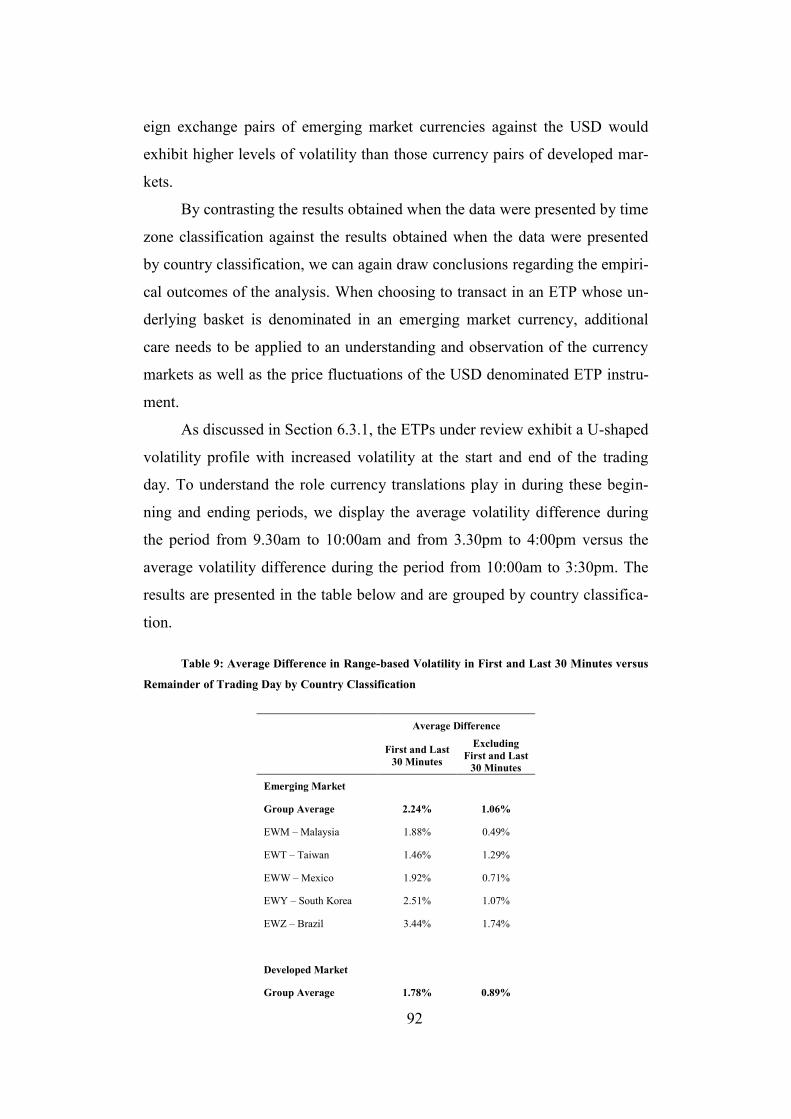
92

eign exchange pairs of emerging market currencies against the USD would

exhibit higher levels of volatility than those currency pairs of developed mar-

kets.

By contrasting the results obtained when the data were presented by time

zone classification against the results obtained when the data were presented

by country classification, we can again draw conclusions regarding the empiri-

cal outcomes of the analysis. When choosing to transact in an ETP whose un-

derlying basket is denominated in an emerging market currency, additional

care needs to be applied to an understanding and observation of the currency

markets as well as the price fluctuations of the USD denominated ETP instru-

ment.

As discussed in Section 6.3.1, the ETPs under review exhibit a U-shaped

volatility profile with increased volatility at the start and end of the trading

day. To understand the role currency translations play in during these begin-

ning and ending periods, we display the average volatility difference during

the period from 9.30am to 10:00am and from 3.30pm to 4:00pm versus the

average volatility difference during the period from 10:00am to 3:30pm. The

results are presented in the table below and are grouped by country classifica-

tion.

Table 9: Average Difference in Range-based Volatility in First and Last 30 Minutes versus

Remainder of Trading Day by Country Classification

Average Difference

First and Last 30 Minutes

Excluding First and Last

30 Minutes

Emerging Market


EWM – Malaysia 1.88% 0.49%

EWT – Taiwan 1.46% 1.29%

EWW – Mexico 1.92% 0.71%

EWY – South Korea 2.51% 1.07%

EWZ – Brazil 3.44% 1.74%

Developed Market


93

EWA – Australia 1.94% 0.96%

EWC – Canada 2.19% 0.96%

EWD – Sweden 2.41% 0.85%

EWG – Germany 2.75% 0.75%

EWH – Hong Kong 2.15% 1.10%

EWI – Italy 0.87% 0.60%

EWJ – Japan 1.38% 0.84%

EWK – Belgium 2.85% 1.40%



EWO – Austria 1.94% 0.99%

EWP – Spain 0.73% 0.60%

EWQ – France 0.59% 0.49%

EWS – Singapore 1.93% 1.10%


Reviewing the data in Table 9 provides additional insight into the mech-

anisms at work. It is clear that decomposing the trading day periods into the

first and last 30 minutes in the trading day versus the remainder of the trading

day indicates that the impact of currency translation on range-based volatility

is particularly noticeable at the beginning and end of the trading session. This

effect is not only prevalent in emerging market currencies, but also in devel-

oped market currencies, with the increase in initial and final range-based vola-

tility meaningful for ETPs with underlying baskets listed in Canada, Sweden,

Germany, Hong Kong, Belgium, and the United Kingdom.

It suggests that the trading of ETPs with foreign underlying baskets at

the start or end of the trading day is best avoided unless deeper awareness of

the foreign exchange market environment is also incorporated into the trading

decision making process.

94

Chapter 9

9 Conclusion

The research objective of this thesis was to conduct an empirical analy-

sis of the effects on ETP price volatility that result when the ETP instrument is

listed on an exchange that is in a different time zone to that of the underlying

securities basket.

Recalling the study of Chan, Fong, Kho and Stulz (1996) who found that

Japanese and European equities were most volatile during the US morning

trading session and that of Chelley-Steeley and Park (2011) who found periods

following a market closure were 20% more volatile than during regular peri-

ods, this thesis concludes that the US morning session does indeed present a

higher volatility trading environment for not just equity securities but also for

ETPs. The findings of this thesis confirm and support the findings of the prior,

related literature. ETPs do exhibit increased volatility at the start of the US

trading session and show a U-shaped volatility profile.

In the examination of the Flash Crash in Section 6.3.2.1 which provided

an extreme view of the impact on ETP prices during a brief crisis period,

Madhavan (2012) found that due to the distortion in equity prices that made up

the underlying ETP baskets, there was an interruption in the natural arbitrage

mechanisms which work to maintain ETP prices close to NAV. This interrup-

tion pushed ETP prices far from NAV and was a particularly volatilite period.

The interruption in the natural arbitrage mechanism is always present for the

non-synchronous ETP group and for part of the US trading day for partially-

synchronous ETPs.

In addition to the U-shaped volatility profile, the ETPs from the partially

synchronous group undergo a “regime shift” during the transition period of an

open to a closed underlying market during the US trading morning. This find-

95

ing is supportive of the study conducted by Levy and Lieberman (2013) who

also found a change in the primary price driver for European ETPs as the un-

derlying European markets closed.

From a practitioner’s perspective, increased volatility in prices for the

partially synchronous group suggests far greater care needs to be applied when

transacting in these instruments It is determined that the range-based volatility

measured in the currency of the underlying securities is lower than that meas-

ured in USD. This indicates that the process of translating the NAV of the un-

derlying basket into USD for the purpose of a USD NAV computation and

USD denominated intraday pricing, introduces additional volatility.

Additionally, decomposing the trading day periods into the first and last

30 minutes in the trading day versus the remainder of the trading day indicates

that the impact of currency translation on range-based volatility is particularly

noticeable at the beginning and end of the trading session. This effect is not

only prevalent in emerging market currencies, but also in developed market

currencies.

These findings taken together emphasise the importance of the timing of

trade execution when transacting in ETPs with foreign underlying security

baskets. ETPs are undoubtedly useful instruments for institutional and retail

investors, materially reducing the transactional cost and complexity of gaining

investment exposure to foreign markets. For investors with medium to long

term investment time horizons, increased volatility at the start or end of the

trading day, or indeed for European ETPs during the European market close, is

unlikely to create a material investment performance effect over the time hori-

zon. However, for short-term market participants, the increased volatility dur-

ing these periods could materially affect investment performance.

Irrespective of investment time horizon, it is prudent for those investors

transacting in foreign ETPs to do so during periods in the market when volatil-

ity is typically low and price certainty is high.

96

Bibliography

Admati, A. R. & Pfleiderer, P., 1998. A theory of intraday patterns:

volume and price variability. The Review of Financial Studies, 1(1), pp. 3-40.

Agarwal, S., Liu, C. & Rhee, S. G., 2007. Where does price discovery

occur for stocks traded in multiple markets? Evidence from Hong Kong and

London. Journal of International Money and Finance, Volume 26, pp. 46-63.

Alizadeh, S., Brandt, M. W. & Diebold, F. X., 2002. Range-based

estimation of stochastic volatility models. Journal of Finance, p. 1047–1092.

Anderson, T. G., Bollerslev, T., Diebold, F. X. & Labys, P., 2001. The

Distribution of Realized Exchange Rate Volatility. Journal of the American

Statistical Association, Volume 96, pp. 42-55.

Baltagi, B., 2011. Econometrics. 5 ed. New York: Springer Science &

Business Media.

Bennett, C. & Gil, M. A., 2012. Measuring Historical Volatility, Madrid:

Santander Global Banking and Markets.

BlackRock Inc, 2013. Exchange Traded Products: Overview, Benefits

and Myths, s.l.: s.n.

Brandt, M. W. & Diebold, F. X., 2006. A no-arbitrage approach to

range-based estimation of return covariances and correlations. Journal of

Business, Volume 79, p. 61–74.

Chan, K. C., Fong, W.-M., Kho, B.-C. & Stulz, R. M., 1996.

Information, trading and stock returns: Lessons from dually-listed securities.

Journal of Banking & Finance, Volume 20, pp. 1161-1187.

Chelley-Steeley, P. & Park, K., 2011. Intraday patterns in London listed

Exchange Traded Funds. International Review of Financial Analysis, Volume

20, p. 244–251.

Chou, R. Y., Chou, H.-c. & Liu, N., 2009. Range Volatility Models and

Their Applications in Finance. In: The Handbook of Quantitative Finance and

Risk Management. s.l.:Springer.

Easley, D., Lopez de Prado, M. M. & O'Hara, M., 2011. The

Microstructure of the "Flash Crash": Flow Toxicity, Liquidity Crashes, and the

97

Probability of Informed Trading. The Journal of Portfolio Management, 37(2),

pp. 118-128.

Engle, R. & Sarkar, D., 2002. Pricing Exchange Traded Funds, s.l.: s.n.

Engle, R. & Sarkar, D., 2006. Premiums-Discounts and Exchange

Traded Funds. The Journal of Derivatives, p. 27.

Eun, C. S. & Sabherwal, S., 2003. Cross-Border Listings and Price

Discovery: Evidence from U.S.-Listed Canadian Stocks. The Journal of

Finance, 58(2), pp. 549-575.

Eviews 8 Users Guide I, 2014. Users Guide I, s.l.: IHS Global Inc.

Feller, W., 1951. The asymtotic distribution of the range of sums of

independent random variables. The Annals of Mathematical Statistics,

September, 22(3), pp. 427-432.

Foster, D. & Viswanathan, 1993. Variation in trading volatility, and

trading costs: Evidence on recent price formation models. The Journal of

Finance, Volume 48, pp. 187-211.

Fuhr, D., 2014. ETFGI LLP. [Online]

Available at: http://www.etfgi.com/publications/reports/reportid/453

[Accessed 15 July 2014].

Fuller, W. A. & Dickey, D. A., 1979. Distribution of the Estimators for

Autoregressive Time Series With a Unit Root. Journal of the American

Statistical Association, 74(366), pp. 427-431.

Garman, M. B. & Klaas, M. J., 1980. On the estimation of security price

volatilities from historical data. Journal of Business, Volume 53, pp. 67-78.

Gastineau, G. L., 2001. An Introduction to Exchange-Traded Funds

(ETFs). Journal of Portfolio Management.

Grammig, J., Melvin, M. & Schlag, C., 2005. Internationally cross-listed

stock prices during overlapping trading hours: price discovery and exchange

rate effects. Journal of Empirical Finance, Volume 12, pp. 139-164.

Guedj, I. & Huang, J., 2008. Are ETFs Replacing Index Mutual Funds?,

s.l.: s.n.

Hamm, S. J. W., 2010. The Effect of ETFs on Stock Liquidity,

Pennsylvania: University of Pennsylvania.

98

Hughen, J. C. & Mathew, P. G., 2009. The efficiency of international

information flow: Evidence from the ETF and CEF prices. International

Review of Financial Analysis, Volume 18, pp. 40-49.

Investment Company Institute, 2014. 2014 Investment Company Fact

Book, s.l.: Investment Company Institute.

Kwiatkowski, D., Phillips , P. C., Schmidt , P. & Shin , Y., 1992. How

sure are we that economic time series have a unit root?. Journal of

Econometrics, Volume 54, pp. 159-178.

Laerd Statistics, n.d. Mann-Whitney U test in SPSS. [Online]

Available at: https://statistics.laerd.com/premium-sample/mwut/mann-

whitney-test-in-spss-2.php

[Accessed 26 April 2015].

Laerd Statistics, n.d. Sign Test using SPSS. [Online]

Available at: https://statistics.laerd.com/spss-tutorials/sign-test-using-spss-

statistics.php

[Accessed 9 May 2015].

Levy, A. & Lieberman, O., 2013. Overreaction of country ETFs to US

market returns: Intraday vs. daily horizons and the role of synchronized

trading. Journal of Banking & Finance, Volume 37, p. 1412–1421.

Madhavan, A., 2012. Exchange-Traded Funds, Market Structure, and the

Flash Crash. Financial Analysts Journal, 68(4), pp. 20-35.

Martens, M. & van Dijk, D., 2007. Measuring volatility with the realized

range. Journal of Econometrics, 138(1), pp. 181-207.

Moulton, P. C. & Wei, L., 2005. A Tale of Two Time Zones: Cross-

Listed Stock Liquidity and the Availability of Substitutes, New York: New

York Stock Exchange.

MSCI Inc, 2014. MSCI Country Classification Standard. [Online]

Available at:

https://www.msci.com/resources/products/indexes/global_equity_indexes/gimi

/stdindex/MSCI_Country_Classification_Standard.pdf


99

MSCI Index Research, 2014. MSCI Global Investable Market Indexes

Methodology, s.l.: s.n.

MSCI Index Research, 2014. MSCI Global Investable Market Indexes

Methodology Summary, s.l.: s.n.

Ng, S. & Perron, P., 1995. Unit Root Tests in ARMA Models with Data-

Dependent Methods for the Selection of the Truncation Lag. Journal of the

American Statistical Association, 90(429), pp. 268-281.

Parkinson, M., 1980. The Extreme Value Method for Estimating the

Variance of the Rate of Return. The Journal of Business, January, 53(1), pp.

61-65.

Petajisto, A., 2013. Inefficiencies in the Pricing of Exchange Traded

Funds, s.l.: s.n.

Phillips, P. C. & Perron, P., 1988. Testing for a unit root in time series

regression. Biometrika, 75(2), pp. 335-346.

Razali, N. M. & Wah, Y. B., 2011. Power comparisons of Shapiro-Wilk,

Kolmogorov-Smirnov, Lilliefors and Anderson-Darling tests. Journal of

Statistical Modeling and Analytics, 2(1), pp. 21-33.

Rompotis, G. G., 2010. Does premium impact Exchange-Traded Funds’

returns? Evidence from iShares. Journal of Asset Management, 11(4), pp. 298-

308.

Rosella, M. R. & Pugliese, D., 2006. The evolution of the exchange

traded fund: is active management on the horizon?. Journal of Investment

Compliance, 7(3), pp. 44-50.

Satchell, S. & Rogers, L., 1991. Estimating variance from High, Low

and Closing Prices. The Annals of Applied Probability, 1(4), pp. 504-512.

Schwert, G. W., 1989. Tests for Unit Roots: A Monte Carlo

Investigation. Journal of Business & Economic Statistics, 7(2), pp. 147-159.

Shamah, S., 2011. A Foreign Exchange Primer. 2, unabridged ed.

s.l.:John Wiley & Sons.

Shu, J. & Zhang, J. E., 2006. Testing Range Estimators of Historical

Volatility. The Journal of Futures Markets, 26(3), pp. 297-313.

100

Staffs of the CFTC and SEC, 2010. Findings Regarding the Market

Events of May 6, 2010, New York: U.S. Commodity Futures Trading

Commission & U.S. Securities & Exchange Commission.

Tannous, G., Wang, J. & Wilson, C., 2013. The Intraday Pattern of

Information Asymmetry, Spread, and Depth: Evidence from the NYSE.

International Review of Finance, 13(2), p. 215–240.

Thadewald, . T. & Büning, H., 2004. Jarque-Bera test and its

competitors for testing normality: A power comparison, Berlin: Free

University Berlin, School of Business & Economics.

Tse, Y. & Martinez, V., 2007. Price discovery and informational

efficiency of international iShares funds. Global Finance Journal, Volume 18,

pp. 1-15.

University of Paris-Sorbonne Economics Centre, na. Choosing the Lag

Length for the ADF Test. [Online]

Available at: http://eurequa.univ-paris1.fr/membres/Ahamada/cours/nsss.pdf


Voraprateep, J., 2013. Robustness of Wilcoxon Signed-Rank Test Against

the Assumption of Symmetry, Birmingham: School of Mathematics, University

of Birmingham.

Yang, D. & Zhang, Q., 2000. Drift-Independent Volatility Estimation

Based on High, Low, Open and Close Prices. Journal of Business, 73(3), pp.

477-491.

Yunus, N., 2013. Contagion in international financial markets: A

recursive cointegration approach. Journal of Multinational Financial

Management, 23(4), pp. 327-337.

Zivot, E., 2006. Economics 584: Time Series Econometrics. [Online]

Available at: http://faculty.washington.edu/ezivot/econ584/econ584.htm

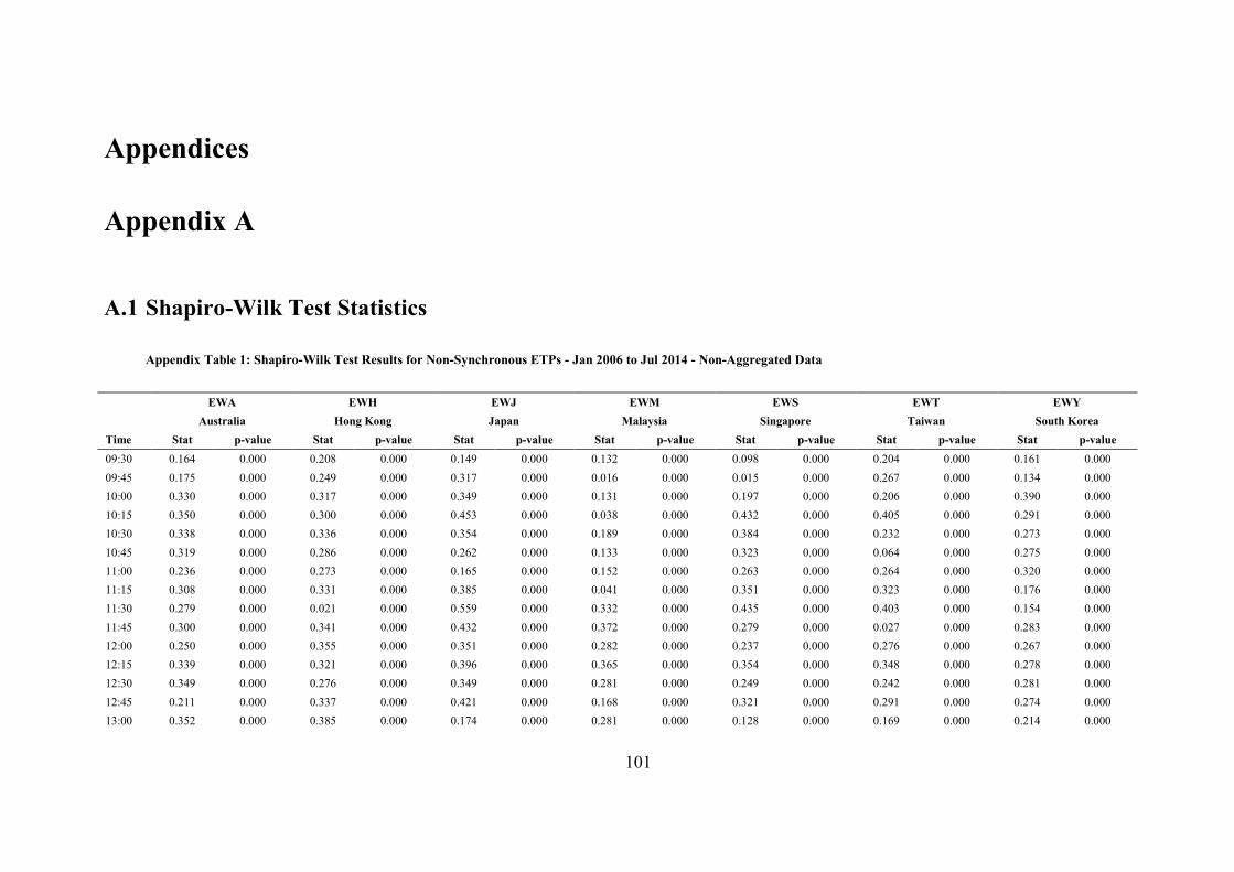
101

Appendices

Appendix A

A.1 Shapiro-Wilk Test Statistics

Appendix Table 1: Shapiro-Wilk Test Results for Non-Synchronous ETPs - Jan 2006 to Jul 2014 - Non-Aggregated Data

EWA EWH EWJ EWM EWS EWT EWY Australia Hong Kong Japan Malaysia Singapore Taiwan South Korea

Time Stat p-value Stat p-value Stat p-value Stat p-value Stat p-value Stat p-value Stat p-value 09:30 0.164 0.000 0.208 0.000 0.149 0.000 0.132 0.000 0.098 0.000 0.204 0.000 0.161 0.000 09:45 0.175 0.000 0.249 0.000 0.317 0.000 0.016 0.000 0.015 0.000 0.267 0.000 0.134 0.000 10:00 0.330 0.000 0.317 0.000 0.349 0.000 0.131 0.000 0.197 0.000 0.206 0.000 0.390 0.000 10:15 0.350 0.000 0.300 0.000 0.453 0.000 0.038 0.000 0.432 0.000 0.405 0.000 0.291 0.000 10:30 0.338 0.000 0.336 0.000 0.354 0.000 0.189 0.000 0.384 0.000 0.232 0.000 0.273 0.000 10:45 0.319 0.000 0.286 0.000 0.262 0.000 0.133 0.000 0.323 0.000 0.064 0.000 0.275 0.000 11:00 0.236 0.000 0.273 0.000 0.165 0.000 0.152 0.000 0.263 0.000 0.264 0.000 0.320 0.000 11:15 0.308 0.000 0.331 0.000 0.385 0.000 0.041 0.000 0.351 0.000 0.323 0.000 0.176 0.000 11:30 0.279 0.000 0.021 0.000 0.559 0.000 0.332 0.000 0.435 0.000 0.403 0.000 0.154 0.000 11:45 0.300 0.000 0.341 0.000 0.432 0.000 0.372 0.000 0.279 0.000 0.027 0.000 0.283 0.000 12:00 0.250 0.000 0.355 0.000 0.351 0.000 0.282 0.000 0.237 0.000 0.276 0.000 0.267 0.000 12:15 0.339 0.000 0.321 0.000 0.396 0.000 0.365 0.000 0.354 0.000 0.348 0.000 0.278 0.000 12:30 0.349 0.000 0.276 0.000 0.349 0.000 0.281 0.000 0.249 0.000 0.242 0.000 0.281 0.000 12:45 0.211 0.000 0.337 0.000 0.421 0.000 0.168 0.000 0.321 0.000 0.291 0.000 0.274 0.000 13:00 0.352 0.000 0.385 0.000 0.174 0.000 0.281 0.000 0.128 0.000 0.169 0.000 0.214 0.000

102


Time Stat p-value Stat p-value Stat p-value Stat p-value Stat p-value Stat p-value Stat p-value 13:15 0.259 0.000 0.319 0.000 0.327 0.000 0.307 0.000 0.323 0.000 0.299 0.000 0.213 0.000 13:30 0.289 0.000 0.311 0.000 0.355 0.000 0.184 0.000 0.218 0.000 0.319 0.000 0.328 0.000 13:45 0.239 0.000 0.138 0.000 0.251 0.000 0.134 0.000 0.125 0.000 0.223 0.000 0.055 0.000 14:00 0.236 0.000 0.226 0.000 0.309 0.000 0.199 0.000 0.225 0.000 0.169 0.000 0.178 0.000 14:15 0.165 0.000 0.254 0.000 0.273 0.000 0.294 0.000 0.301 0.000 0.231 0.000 0.233 0.000 14:30 0.231 0.000 0.314 0.000 0.384 0.000 0.324 0.000 0.281 0.000 0.300 0.000 0.304 0.000 14:45 0.035 0.000 0.312 0.000 0.399 0.000 0.351 0.000 0.325 0.000 0.326 0.000 0.318 0.000 15:00 0.240 0.000 0.292 0.000 0.253 0.000 0.299 0.000 0.089 0.000 0.190 0.000 0.236 0.000 15:15 0.144 0.000 0.158 0.000 0.298 0.000 0.274 0.000 0.299 0.000 0.294 0.000 0.217 0.000 15:30 0.250 0.000 0.121 0.000 0.298 0.000 0.089 0.000 0.233 0.000 0.169 0.000 0.260 0.000 15:45 0.209 0.000 0.188 0.000 0.242 0.000 0.276 0.000 0.222 0.000 0.171 0.000 0.149 0.000

Appendix Table 2: Shapiro-Wilk Test Results for Partially Synchronous ETPs - Jan 2006 to Jul 2014 - Non-Aggregated Data

EWD EWG EWI EWK EWL EWN EWO EWP EWQ EWU Sweden Germany Italy Belgium Switzerland Netherlands Austria Spain France United Kingdom

Time Stat p-value Stat p-value Stat p-value Stat p-value Stat p-value Stat p-value Stat p-value Stat p-value Stat p-value Stat p-value 09:30 0.060 0.000 0.062 0.000 0.280 0.000 0.352 0.000 0.369 0.000 0.258 0.000 0.250 0.000 0.096 0.000 0.262 0.000 0.051 0.000 09:45 0.362 0.000 0.125 0.000 0.142 0.000 0.026 0.000 0.400 0.000 0.047 0.000 0.021 0.000 0.038 0.000 0.266 0.000 0.000 0.000 10:00 0.300 0.000 0.108 0.000 0.116 0.000 0.038 0.000 0.340 0.000 0.197 0.000 0.017 0.000 0.202 0.000 0.343 0.000 0.021 0.000 10:15 0.438 0.000 0.331 0.000 0.281 0.000 0.180 0.000 0.381 0.000 0.280 0.000 0.035 0.000 0.341 0.000 0.369 0.000 0.318 0.000 10:30 0.429 0.000 0.378 0.000 0.434 0.000 0.276 0.000 0.415 0.000 0.303 0.000 0.180 0.000 0.362 0.000 0.322 0.000 0.308 0.000 10:45 0.343 0.000 0.352 0.000 0.510 0.000 0.149 0.000 0.378 0.000 0.245 0.000 0.100 0.000 0.469 0.000 0.457 0.000 0.366 0.000 11:00 0.330 0.000 0.298 0.000 0.385 0.000 0.106 0.000 0.211 0.000 0.095 0.000 0.226 0.000 0.300 0.000 0.275 0.000 0.388 0.000 11:15 0.267 0.000 0.339 0.000 0.289 0.000 0.118 0.000 0.087 0.000 0.039 0.000 0.166 0.000 0.300 0.000 0.294 0.000 0.370 0.000 11:30 0.192 0.000 0.298 0.000 0.386 0.000 0.035 0.000 0.338 0.000 0.108 0.000 0.319 0.000 0.435 0.000 0.416 0.000 0.394 0.000 11:45 0.351 0.000 0.270 0.000 0.400 0.000 0.213 0.000 0.408 0.000 0.359 0.000 0.120 0.000 0.422 0.000 0.374 0.000 0.095 0.000 12:00 0.269 0.000 0.116 0.000 0.437 0.000 0.149 0.000 0.335 0.000 0.204 0.000 0.117 0.000 0.341 0.000 0.263 0.000 0.333 0.000 12:15 0.250 0.000 0.251 0.000 0.355 0.000 0.136 0.000 0.249 0.000 0.255 0.000 0.193 0.000 0.281 0.000 0.271 0.000 0.301 0.000

103

EWD EWG EWI EWK EWL EWN EWO EWP EWQ EWU Sweden Germany Italy Belgium Switzerland Netherlands Austria Spain France United Kingdom

Time Stat p-value Stat p-value Stat p-value Stat p-value Stat p-value Stat p-value Stat p-value Stat p-value Stat p-value Stat p-value 12:30 0.287 0.000 0.111 0.000 0.325 0.000 0.197 0.000 0.308 0.000 0.201 0.000 0.125 0.000 0.185 0.000 0.250 0.000 0.309 0.000 12:45 0.221 0.000 0.261 0.000 0.231 0.000 0.220 0.000 0.214 0.000 0.214 0.000 0.012 0.000 0.338 0.000 0.248 0.000 0.250 0.000 13:00 0.286 0.000 0.309 0.000 0.143 0.000 0.244 0.000 0.343 0.000 0.304 0.000 0.092 0.000 0.377 0.000 0.350 0.000 0.022 0.000 13:15 0.265 0.000 0.305 0.000 0.264 0.000 0.119 0.000 0.091 0.000 0.294 0.000 0.103 0.000 0.014 0.000 0.302 0.000 0.239 0.000 13:30 0.257 0.000 0.315 0.000 0.392 0.000 0.144 0.000 0.324 0.000 0.251 0.000 0.090 0.000 0.285 0.000 0.331 0.000 0.113 0.000 13:45 0.231 0.000 0.149 0.000 0.343 0.000 0.240 0.000 0.155 0.000 0.169 0.000 0.088 0.000 0.161 0.000 0.186 0.000 0.126 0.000 14:00 0.251 0.000 0.254 0.000 0.256 0.000 0.014 0.000 0.286 0.000 0.013 0.000 0.100 0.000 0.359 0.000 0.143 0.000 0.259 0.000 14:15 0.181 0.000 0.175 0.000 0.228 0.000 0.168 0.000 0.293 0.000 0.171 0.000 0.151 0.000 0.208 0.000 0.151 0.000 0.229 0.000 14:30 0.326 0.000 0.265 0.000 0.312 0.000 0.220 0.000 0.242 0.000 0.156 0.000 0.265 0.000 0.299 0.000 0.186 0.000 0.257 0.000 14:45 0.172 0.000 0.228 0.000 0.334 0.000 0.259 0.000 0.304 0.000 0.243 0.000 0.136 0.000 0.341 0.000 0.303 0.000 0.296 0.000 15:00 0.313 0.000 0.265 0.000 0.286 0.000 0.137 0.000 0.217 0.000 0.297 0.000 0.083 0.000 0.184 0.000 0.193 0.000 0.244 0.000 15:15 0.189 0.000 0.226 0.000 0.266 0.000 0.158 0.000 0.221 0.000 0.194 0.000 0.133 0.000 0.286 0.000 0.215 0.000 0.273 0.000 15:30 0.148 0.000 0.133 0.000 0.325 0.000 0.167 0.000 0.088 0.000 0.230 0.000 0.171 0.000 0.253 0.000 0.064 0.000 0.105 0.000 15:45 0.199 0.000 0.185 0.000 0.404 0.000 0.144 0.000 0.177 0.000 0.105 0.000 0.119 0.000 0.025 0.000 0.019 0.000 0.116 0.000

Appendix Table 3: Shapiro-Wilk Test Results for Synchronous ETPs - Jan 2006 to Jul 2014 - Non-Aggregated Data

EWC EWW EWZ IVV Canada Mexico Brazil United States

Time Stat p-value Stat p-value Stat p-value Stat p-value 09:30 0.153 0.000 0.220 0.000 0.205 0.000 0.088 0.000 09:45 0.012 0.000 0.160 0.000 0.302 0.000 0.298 0.000 10:00 0.230 0.000 0.173 0.000 0.290 0.000 0.264 0.000 10:15 0.438 0.000 0.402 0.000 0.078 0.000 0.346 0.000 10:30 0.394 0.000 0.250 0.000 0.311 0.000 0.299 0.000 10:45 0.293 0.000 0.335 0.000 0.310 0.000 0.301 0.000 11:00 0.356 0.000 0.307 0.000 0.295 0.000 0.185 0.000 11:15 0.271 0.000 0.116 0.000 0.268 0.000 0.291 0.000

104

A.2 Jarque-Bera Test Statistics

Appendix Table 4: Jarque-Bera Test Results for Non-Synchronous ETPs - Jan 2006 to Jul 2014 - Non-Aggregated Data

EWA EWH EWJ EWM EWS EWT EWY

Australia Hong Kong Japan Malaysia Singapore Taiwan South Korea Time Stat p-value Stat p-value Stat p-value Stat p-value Stat p-value Stat p-value Stat p-value 09:30 2 202 811 0.000 3 286 839 0.000 10 727 735 0.000 3 306 686 0.000 11 827 378 0.000 6 176 770 0.000 6 575 619 0.000 09:45 38 036 622 0.000 13 047 734 0.000 6 651 724 0.000 389 000 000 0.000 400 000 000 0.000 7 353 405 0.000 80 721 290 0.000 10:00 8 144 329 0.000 5 636 887 0.000 3 186 672 0.000 57 850 890 0.000 11 758 621 0.000 92 056 781 0.000 495 417 0.000

11:30 0.213 0.000 0.296 0.000 0.356 0.000 0.348 0.000 11:45 0.277 0.000 0.420 0.000 0.234 0.000 0.241 0.000 12:00 0.306 0.000 0.348 0.000 0.181 0.000 0.265 0.000 12:15 0.239 0.000 0.324 0.000 0.231 0.000 0.275 0.000 12:30 0.285 0.000 0.365 0.000 0.198 0.000 0.243 0.000 12:45 0.345 0.000 0.346 0.000 0.216 0.000 0.257 0.000 13:00 0.374 0.000 0.249 0.000 0.226 0.000 0.396 0.000 13:15 0.297 0.000 0.250 0.000 0.237 0.000 0.278 0.000 13:30 0.113 0.000 0.161 0.000 0.312 0.000 0.291 0.000 13:45 0.230 0.000 0.139 0.000 0.148 0.000 0.080 0.000 14:00 0.260 0.000 0.275 0.000 0.217 0.000 0.170 0.000 14:15 0.233 0.000 0.131 0.000 0.190 0.000 0.221 0.000 14:30 0.253 0.000 0.253 0.000 0.025 0.000 0.288 0.000 14:45 0.300 0.000 0.308 0.000 0.141 0.000 0.265 0.000 15:00 0.240 0.000 0.161 0.000 0.175 0.000 0.211 0.000 15:15 0.199 0.000 0.132 0.000 0.253 0.000 0.260 0.000 15:30 0.125 0.000 0.147 0.000 0.085 0.000 0.122 0.000 15:45 0.176 0.000 0.064 0.000 0.101 0.000 0.178 0.000

105


Time Stat p-value Stat p-value Stat p-value Stat p-value Stat p-value Stat p-value Stat p-value 10:15 1 417 314 0.000 1 870 174 0.000 647 649 0.000 243 000 000 0.000 271 818 0.000 376 934 0.000 7 815 086 0.000 10:30 1 789 207 0.000 2 910 807 0.000 1 166 543 0.000 45 472 157 0.000 436 352 0.000 31 170 406 0.000 1 951 411 0.000 10:45 1 149 194 0.000 8 923 559 0.000 9 093 189 0.000 73 650 096 0.000 2 153 547 0.000 254 000 000 0.000 2 876 612 0.000 11:00 8 417 762 0.000 15 165 975 0.000 95 005 291 0.000 54 545 113 0.000 9 716 901 0.000 3 489 588 0.000 1 037 331 0.000 11:15 863 779 0.000 1 232 577 0.000 532 699 0.000 324 000 000 0.000 975 566 0.000 1 523 530 0.000 59 729 144 0.000 11:30 7 680 758 0.000 387 000 000 0.000 71 036 0.000 1 347 527 0.000 500 197 0.000 474 379 0.000 64 135 431 0.000 11:45 6 486 551 0.000 3 853 406 0.000 375 288 0.000 1 422 954 0.000 8 382 666 0.000 366 000 000 0.000 2 956 062 0.000 12:00 9 494 320 0.000 1 551 654 0.000 4 472 865 0.000 4 822 050 0.000 15 760 749 0.000 6 780 722 0.000 4 094 272 0.000 12:15 1 223 574 0.000 1 253 832 0.000 879 400 0.000 755 604 0.000 749 053 0.000 603 179 0.000 1 313 232 0.000 12:30 517 560 0.000 3 085 555 0.000 902 609 0.000 7 585 990 0.000 10 987 781 0.000 14 262 048 0.000 3 581 248 0.000 12:45 8 433 300 0.000 987 395 0.000 307 278 0.000 63 187 492 0.000 1 193 907 0.000 1 727 077 0.000 1 867 348 0.000 13:00 2 412 294 0.000 489 893 0.000 114 000 000 0.000 5 077 222 0.000 149 000 000 0.000 54 753 983 0.000 26 148 574 0.000 13:15 11 767 036 0.000 1 436 390 0.000 3 344 622 0.000 2 367 978 0.000 1 595 788 0.000 1 497 635 0.000 6 255 117 0.000 13:30 3 561 924 0.000 1 983 066 0.000 1 363 728 0.000 30 669 366 0.000 18 887 588 0.000 1 156 433 0.000 621 809 0.000 13:45 4 798 631 0.000 62 267 548 0.000 15 155 503 0.000 58 794 360 0.000 110 000 000 0.000 10 538 679 0.000 281 000 000 0.000 14:00 8 391 449 0.000 10 994 046 0.000 3 373 510 0.000 10 917 342 0.000 11 366 437 0.000 37 446 719 0.000 12 372 722 0.000 14:15 23 194 409 0.000 1 930 373 0.000 3 720 495 0.000 807 963 0.000 1 094 015 0.000 5 174 471 0.000 2 397 526 0.000 14:30 2 315 656 0.000 796 410 0.000 345 448 0.000 642 877 0.000 1 810 225 0.000 959 306 0.000 828 861 0.000 14:45 328 000 000 0.000 790 080 0.000 647 327 0.000 367 722 0.000 1 420 207 0.000 407 043 0.000 1 025 498 0.000 15:00 1 603 360 0.000 764 508 0.000 7 239 153 0.000 1 094 936 0.000 185 000 000 0.000 8 833 742 0.000 2 820 076 0.000 15:15 36 778 745 0.000 64 809 758 0.000 1 788 345 0.000 1 990 074 0.000 1 368 220 0.000 1 088 474 0.000 15 868 183 0.000 15:30 2 286 220 0.000 43 984 406 0.000 2 901 717 0.000 165 000 000 0.000 4 186 171 0.000 34 570 909 0.000 1 057 541 0.000 15:45 3 202 676 0.000 29 328 354 0.000 2 746 099 0.000 1 423 821 0.000 9 608 140 0.000 6 272 382 0.000 28 477 634 0.000

106

Appendix Table 5: Jarque-Bera Test Results for Partially Synchronous ETPs - Jan 2006 to Jul 2014 - Non-Aggregated Data

EWD EWG EWI EWK EWL Sweden Germany Italy Belgium Switzerland

Time Stat p-value Stat p-value Stat p-value Stat p-value Stat p-value 09:30 820 392 0.000 3 816 252 0.000 684 702 0.000 1 413 0.000 169 834 0.000 09:45 2 233 115 0.000 64 648 494 0.000 59 848 727 0.000 128 000 000 0.000 1 170 810 0.000 10:00 2 191 123 0.000 184 000 000 0.000 144 000 000 0.000 99 630 755 0.000 2 082 570 0.000 10:15 297 996 0.000 1 678 955 0.000 7 065 420 0.000 11 580 037 0.000 785 038 0.000 10:30 360 550 0.000 2 038 226 0.000 287 963 0.000 881 732 0.000 893 678 0.000 10:45 1 615 849 0.000 2 016 945 0.000 107 792 0.000 14 220 328 0.000 332 044 0.000 11:00 2 423 748 0.000 1 772 389 0.000 740 911 0.000 19 205 595 0.000 21 786 148 0.000 11:15 13 130 599 0.000 598 616 0.000 12 792 835 0.000 21 751 229 0.000 192 000 000 0.000 11:30 36 189 990 0.000 2 877 604 0.000 574 179 0.000 100 000 000 0.000 908 006 0.000 11:45 930 745 0.000 7 856 965 0.000 421 409 0.000 6 979 912 0.000 643 690 0.000 12:00 8 761 179 0.000 158 000 000 0.000 239 831 0.000 19 175 693 0.000 1 545 909 0.000 12:15 2 851 952 0.000 2 042 949 0.000 534 534 0.000 16 247 856 0.000 9 364 082 0.000 12:30 1 465 048 0.000 95 217 283 0.000 1 207 060 0.000 3 449 118 0.000 1 355 550 0.000 12:45 5 728 669 0.000 3 175 605 0.000 11 607 404 0.000 5 276 968 0.000 7 355 242 0.000 13:00 1 779 118 0.000 5 977 808 0.000 61 923 054 0.000 1 522 883 0.000 1 585 974 0.000 13:15 7 612 346 0.000 1 863 281 0.000 1 618 162 0.000 14 885 832 0.000 111 000 000 0.000 13:30 2 772 852 0.000 2 237 471 0.000 239 186 0.000 24 592 200 0.000 521 418 0.000 13:45 9 525 546 0.000 64 807 036 0.000 760 345 0.000 784 671 0.000 49 421 800 0.000 14:00 6 209 207 0.000 3 165 648 0.000 12 902 479 0.000 85 228 688 0.000 1 085 196 0.000 14:15 10 006 751 0.000 13 307 012 0.000 3 595 308 0.000 3 018 079 0.000 992 298 0.000 14:30 427 262 0.000 2 192 317 0.000 511 131 0.000 3 250 742 0.000 1 749 763 0.000 14:45 15 859 879 0.000 5 565 394 0.000 1 433 009 0.000 1 899 432 0.000 865 499 0.000 15:00 839 293 0.000 2 105 227 0.000 1 332 157 0.000 10 215 189 0.000 4 557 920 0.000 15:15 13 085 413 0.000 4 548 679 0.000 2 715 573 0.000 5 698 294 0.000 15 112 485 0.000 15:30 34 146 866 0.000 32 508 620 0.000 1 851 080 0.000 4 853 071 0.000 151 000 000 0.000 15:45 13 560 342 0.000 9 238 213 0.000 613 711 0.000 16 978 301 0.000 33 323 928 0.000

107

EWN EWO EWP EWQ EWU Netherlands Austria Spain France United Kingdom

Time Stat p-value Stat p-value Stat p-value Stat p-value Stat p-value 09:30 56 958 0.000 15 664 0.000 1 595 130 0.000 382 409 0.000 11 513 163 0.000 09:45 75 752 849 0.000 223 000 000 0.000 189 000 000 0.000 4 689 522 0.000 NA NA 10:00 16 875 983 0.000 206 000 000 0.000 16 192 813 0.000 6 395 407 0.000 385 000 000 0.000 10:15 1 937 133 0.000 49 935 342 0.000 2 511 555 0.000 710 080 0.000 2 434 521 0.000 10:30 7 394 073 0.000 29 618 487 0.000 2 416 901 0.000 1 401 808 0.000 5 772 136 0.000 10:45 4 939 760 0.000 30 124 169 0.000 353 339 0.000 204 151 0.000 925 462 0.000 11:00 101 000 000 0.000 3 908 485 0.000 2 474 959 0.000 4 604 680 0.000 478 518 0.000 11:15 143 000 000 0.000 24 049 990 0.000 10 360 107 0.000 2 887 301 0.000 721 080 0.000 11:30 60 100 383 0.000 984 898 0.000 280 223 0.000 417 861 0.000 1 067 093 0.000 11:45 460 355 0.000 36 232 583 0.000 431 946 0.000 873 704 0.000 201 000 000 0.000 12:00 1 892 512 0.000 20 365 334 0.000 531 493 0.000 1 859 381 0.000 1 635 434 0.000 12:15 956 302 0.000 1 841 832 0.000 2 204 049 0.000 7 469 653 0.000 3 815 263 0.000 12:30 4 978 703 0.000 40 267 184 0.000 24 265 504 0.000 2 210 620 0.000 1 692 966 0.000 12:45 5 106 368 0.000 145 000 000 0.000 946 251 0.000 9 379 270 0.000 2 413 183 0.000 13:00 424 893 0.000 11 724 039 0.000 324 513 0.000 482 995 0.000 353 000 000 0.000 13:15 777 115 0.000 9 416 626 0.000 290 000 000 0.000 995 269 0.000 2 749 936 0.000 13:30 1 002 642 0.000 21 634 912 0.000 3 382 682 0.000 689 797 0.000 105 000 000 0.000 13:45 5 747 903 0.000 51 653 083 0.000 29 651 588 0.000 12 864 528 0.000 33 551 296 0.000 14:00 148 000 000 0.000 12 932 655 0.000 912 295 0.000 31 006 580 0.000 4 440 781 0.000 14:15 4 677 242 0.000 16 280 053 0.000 4 585 292 0.000 8 354 998 0.000 2 311 694 0.000 14:30 4 731 774 0.000 2 469 216 0.000 696 105 0.000 23 920 374 0.000 2 799 463 0.000 14:45 1 311 098 0.000 9 564 516 0.000 513 076 0.000 1 291 624 0.000 1 983 610 0.000 15:00 1 406 567 0.000 88 185 464 0.000 17 237 657 0.000 5 368 265 0.000 3 423 579 0.000 15:15 3 235 198 0.000 11 281 048 0.000 2 726 354 0.000 6 834 811 0.000 2 532 291 0.000 15:30 1 207 786 0.000 3 804 934 0.000 3 373 269 0.000 128 000 000 0.000 49 509 858 0.000 15:45 26 103 674 0.000 26 345 006 0.000 339 000 000 0.000 342 000 000 0.000 94 125 204 0.000

108

Appendix Table 6: Jarque-Bera Test Results for Synchronous ETPs - Jan 2006 to Jul 2014 - Non-Aggregated Data

EWC EWW EWZ IVV

Canada Mexico Brazil United States

Stat p-value Stat p-value Stat p-value Stat p-value 09:30 2 740 355 0.000 2 646 993 0.000 2 376 556 0.000 76 211 438 0.000 09:45 401 000 000 0.000 46 187 720 0.000 2 106 877 0.000 2 044 213 0.000 10:00 34 061 556 0.000 76 496 189 0.000 8 811 558 0.000 16 670 291 0.000 10:15 316 871 0.000 995 941 0.000 119 000 000 0.000 998 469 0.000 10:30 1 578 536 0.000 13 550 429 0.000 609 524 0.000 4 878 438 0.000 10:45 7 331 711 0.000 1 535 539 0.000 646 039 0.000 1 534 465 0.000 11:00 753 550 0.000 1 333 893 0.000 939 478 0.000 15 848 761 0.000 11:15 4 027 729 0.000 137 000 000 0.000 1 401 980 0.000 1 012 070 0.000 11:30 72 963 548 0.000 3 455 703 0.000 322 688 0.000 728 519 0.000 11:45 4 693 002 0.000 769 146 0.000 2 521 640 0.000 18 302 497 0.000 12:00 2 715 551 0.000 3 245 765 0.000 8 030 243 0.000 11 874 743 0.000 12:15 2 816 820 0.000 1 867 954 0.000 5 000 127 0.000 3 891 857 0.000 12:30 1 785 631 0.000 769 418 0.000 3 812 307 0.000 5 453 998 0.000 12:45 1 289 522 0.000 509 701 0.000 11 227 518 0.000 2 714 163 0.000 13:00 836 524 0.000 19 125 772 0.000 3 569 040 0.000 201 767 0.000 13:15 2 012 497 0.000 6 192 556 0.000 2 356 345 0.000 2 397 452 0.000 13:30 109 000 000 0.000 73 490 299 0.000 429 202 0.000 915 097 0.000 13:45 8 417 292 0.000 64 568 581 0.000 21 887 249 0.000 173 000 000 0.000 14:00 9 293 441 0.000 2 653 162 0.000 2 681 732 0.000 23 259 477 0.000 14:15 1 921 785 0.000 103 000 000 0.000 7 134 466 0.000 4 331 092 0.000 14:30 2 213 761 0.000 12 323 468 0.000 82 467 787 0.000 868 402 0.000 14:45 890 919 0.000 2 729 418 0.000 58 223 593 0.000 1 823 836 0.000 15:00 3 075 539 0.000 10 455 770 0.000 4 111 640 0.000 4 591 690 0.000 15:15 15 733 713 0.000 76 934 731 0.000 1 265 031 0.000 2 820 379 0.000 15:30 106 000 000 0.000 68 781 139 0.000 23 025 727 0.000 90 580 300 0.000 15:45 7 788 931 0.000 103 000 000 0.000 12 646 404 0.000 17 495 478 0.000

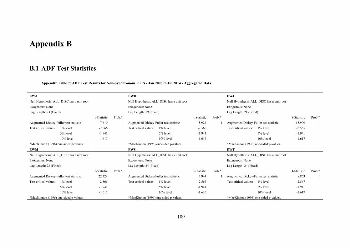
109

Appendix B

B.1 ADF Test Statistics

Appendix Table 7: ADF Test Results for Non-Synchronous ETPs - Jan 2006 to Jul 2014 - Aggregated Data

EWA

EWH

EWJ Null Hypothesis: ALL_DISC has a unit root

Null Hypothesis: ALL_DISC has a unit root


Exogenous: None

Exogenous: None

Exogenous: None Lag Length: 23 (Fixed)

Lag Length: 19 (Fixed)


t-Statistic Prob.*

t-Statistic Prob.*

t-Statistic Prob.* Augmented Dickey-Fuller test statistic 7.610 1 Augmented Dickey-Fuller test statistic 18.924 1 Augmented Dickey-Fuller test statistic 15.909 1 Test critical values: 1% level

-2.566

Test critical values: 1% level

-2.565


-2.565

5% level

-1.941

5% level

-1.941

5% level

-1.941

10% level

-1.617

10% level

-1.617

10% level

-1.617

*MacKinnon (1996) one-sided p-values.


*MacKinnon (1996) one-sided p-values. EWM

EWS

EWT



Null Hypothesis: ALL_DISC has a unit root Exogenous: None

Exogenous: None

Exogenous: None




t-Statistic Prob.*

t-Statistic Prob.*

t-Statistic Prob.*

Augmented Dickey-Fuller test statistic 22.324 1 Augmented Dickey-Fuller test statistic 7.944 1 Augmented Dickey-Fuller test statistic 8.863 1 Test critical values: 1% level

-2.566


-2.567


-2.567

5% level

-1.941

5% level

-1.941

5% level

-1.941

10% level

-1.617

10% level

-1.616

10% level

-1.617




110

EWY Null Hypothesis: ALL_DISC has a unit root Exogenous: None Lag Length: 24 (Fixed)

t-Statistic Prob.* Augmented Dickey-Fuller test statistic 0.881 0.8988 Test critical values: 1% level -2.567

5% level -1.941 10% level -1.617


Appendix Table 8: ADF Test Results for Partially Synchronous ETPs - Jan 2006 to Jul 2014 - Aggregated Data

EWD EWG EWI Null Hypothesis: ALL_DISC has a unit root Null Hypothesis: ALL_DISC has a unit root Null Hypothesis: ALL_DISC has a unit root Exogenous: None Exogenous: None Exogenous: None Lag Length: 24 (Fixed) Lag Length: 22 (Fixed) Lag Length: 23 (Fixed)

t-Statistic Prob.* t-Statistic Prob.* t-Statistic Prob.* Augmented Dickey-Fuller test statistic 3.770 1 Augmented Dickey-Fuller test statistic 15.196 1 Augmented Dickey-Fuller test statistic 1.596 0.9734 Test critical values: 1% level -2.576 Test critical values: 1% level -2.565 Test critical values: 1% level -2.567

5% level -1.942 5% level -1.941 5% level -1.941 10% level -1.616 10% level -1.617 10% level -1.617

*MacKinnon (1996) one-sided p-values. *MacKinnon (1996) one-sided p-values. *MacKinnon (1996) one-sided p-values.

EWK EWL EWN Null Hypothesis: ALL_DISC has a unit root Null Hypothesis: ALL_DISC has a unit root Null Hypothesis: ALL_DISC has a unit root Exogenous: None Exogenous: None Exogenous: None Lag Length: 22 (Fixed) Lag Length: 24 (Fixed) Lag Length: 23 (Fixed)

t-Statistic Prob.* t-Statistic Prob.* t-Statistic Prob.* Augmented Dickey-Fuller test statistic 3.440 0.9999 Augmented Dickey-Fuller test statistic 2.036 0.9903 Augmented Dickey-Fuller test statistic -0.386 0.5448 Test critical values: 1% level -2.568 Test critical values: 1% level -2.574 Test critical values: 1% level -2.570

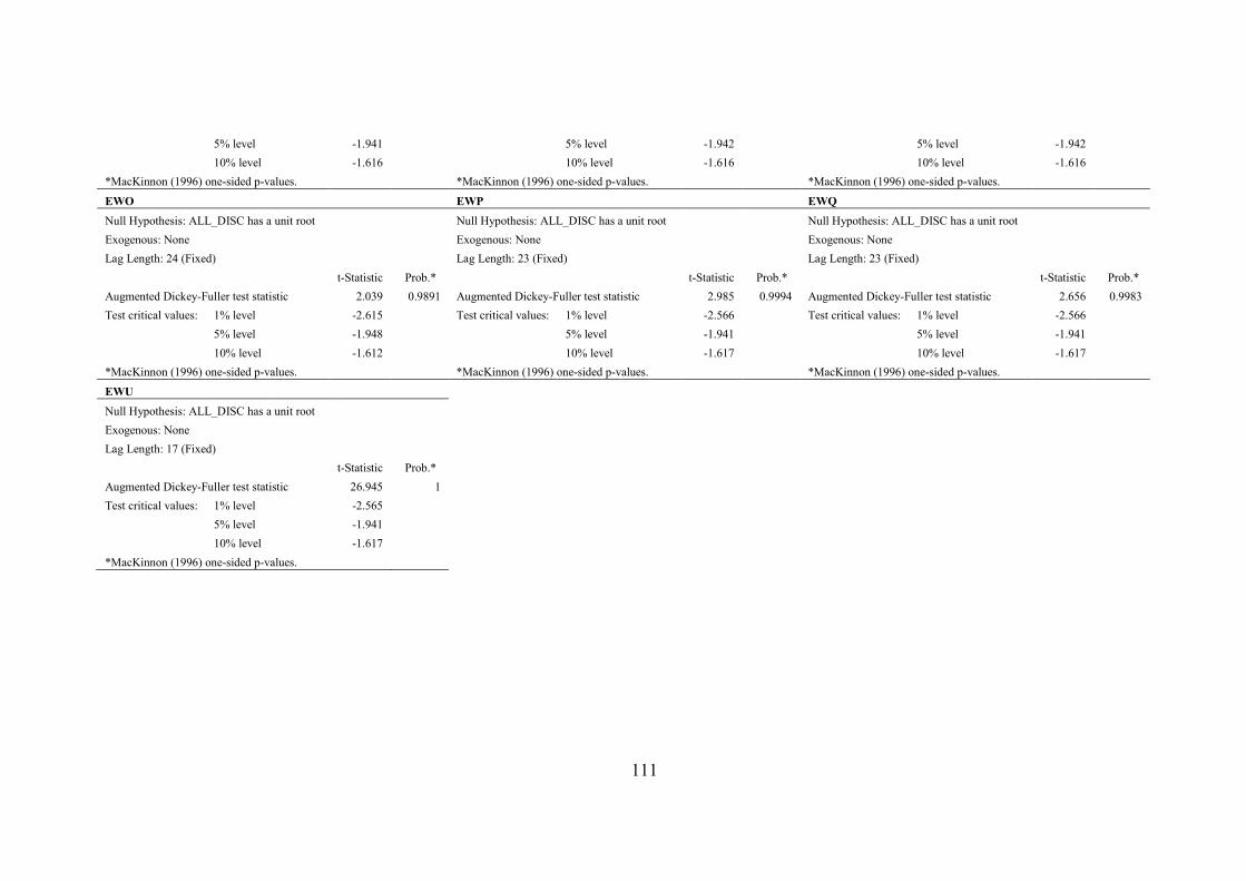
111

5% level

-1.941

5% level

-1.942

5% level

-1.942

10% level

-1.616

10% level

-1.616

10% level

-1.616 *MacKinnon (1996) one-sided p-values.



EWO EWP EWQ Null Hypothesis: ALL_DISC has a unit root



Exogenous: None

Exogenous: None

Exogenous: None Lag Length: 24 (Fixed)



t-Statistic Prob.*

t-Statistic Prob.*

t-Statistic Prob.* Augmented Dickey-Fuller test statistic 2.039 0.9891 Augmented Dickey-Fuller test statistic 2.985 0.9994 Augmented Dickey-Fuller test statistic 2.656 0.9983 Test critical values: 1% level

-2.615


-2.566


-2.566

5% level

-1.948

5% level

-1.941

5% level

-1.941

10% level

-1.612

10% level

-1.617

10% level

-1.617



*MacKinnon (1996) one-sided p-values. EWU

Null Hypothesis: ALL_DISC has a unit root Exogenous: None


t-Statistic Prob.*

Augmented Dickey-Fuller test statistic 26.945 1 Test critical values: 1% level

-2.565

5% level

-1.941

10% level

-1.617


112

Appendix Table 9: ADF Test Results for Synchronous ETPs - Jan 2006 to Jul 2014 - Aggregated Data

IVV EWC EWW Null Hypothesis: ALL_DISC has a unit root Null Hypothesis: ALL_DISC has a unit root Null Hypothesis: ALL_DISC has a unit root Exogenous: None Exogenous: None Exogenous: None Lag Length: 24 (Fixed) Lag Length: 24 (Fixed) Lag Length: 23 (Fixed)

t-Statistic Prob.* t-Statistic Prob.* t-Statistic Prob.* Augmented Dickey-Fuller test statistic 4.251 1 Augmented Dickey-Fuller test statistic 1.080 0.9274 Augmented Dickey-Fuller test statistic 12.770 1 Test critical values: 1% level -2.566 Test critical values: 1% level -2.567 Test critical values: 1% level -2.566



EWZ Null Hypothesis: ALL_DISC has a unit root Exogenous: None Lag Length: 24 (Fixed)

t-Statistic Prob.* Augmented Dickey-Fuller test statistic 9.811 1 Test critical values: 1% level -2.566

5% level -1.941 10% level -1.617


113

B.2 Phillips-Perron Test Statistics

Appendix Table 10: Phillips-Perron Test Results for Non-Synchronous ETPs - Jan 2006 to Jul 2014 - Aggregated Data

EWA EWH EWJ Null Hypothesis: ALL_DISC has a unit root Null Hypothesis: ALL_DISC has a unit root Null Hypothesis: ALL_DISC has a unit root Exogenous: None Exogenous: None Exogenous: None Bandwidth: 155 (Newey-West automatic) using Bartlett kernel Bandwidth: 150 (Newey-West automatic) using Bartlett kernel Bandwidth: 157 (Newey-West automatic) using Bartlett kernel

Adj. t-Stat Prob.* Adj. t-Stat Prob.*

Adj. t-Stat Prob.*

Phillips-Perron test statistic -363.586 0.0001 Phillips-Perron test statistic -372.836 0.0001 Phillips-Perron test statistic -363.059 0.0001

Test critical values: 1% level -2.565 Test critical val-ues: 1% level -2.565

Test critical val-ues: 1% level -2.565

5% level -1.941 5% level -1.941 5% level -1.941

10% level -1.617 10% level -1.617

10% level -1.617


EWM EWS EWT Null Hypothesis: ALL_DISC has a unit root Null Hypothesis: ALL_DISC has a unit root Null Hypothesis: ALL_DISC has a unit root Exogenous: None Exogenous: None Exogenous: None Bandwidth: 91 (Newey-West automatic) using Bartlett kernel Bandwidth: 101 (Newey-West automatic) using Bartlett kernel Bandwidth: 152 (Newey-West automatic) using Bartlett kernel


Adj. t-Stat Prob.*





10% level -1.617 10% level -1.617

10% level -1.617


114

EWY Null Hypothesis: ALL_DISC has a unit root Exogenous: None Bandwidth: 154 (Newey-West automatic) using Bartlett kernel

Adj. t-Stat Prob.* Phillips-Perron test statistic -396.220 0.0001 Test critical values: 1% level -2.565

5% level -1.941 10% level -1.617


Appendix Table 11: Phillips-Perron Test Results for Partially Synchronous ETPs - Jan 2006 to Jul 2014 - Aggregated Data

EWD EWG EWI Null Hypothesis: ALL_DISC has a unit root Null Hypothesis: ALL_DISC has a unit root Null Hypothesis: ALL_DISC has a unit root Exogenous: None Exogenous: None Exogenous: None Bandwidth: 147 (Newey-West automatic) using Bartlett kernel Bandwidth: 159 (Newey-West automatic) using Bartlett kernel Bandwidth: 133 (Newey-West automatic) using Bartlett kernel


Adj. t-Stat Prob.*





10% level -1.617 10% level -1.62

10% level -1.617


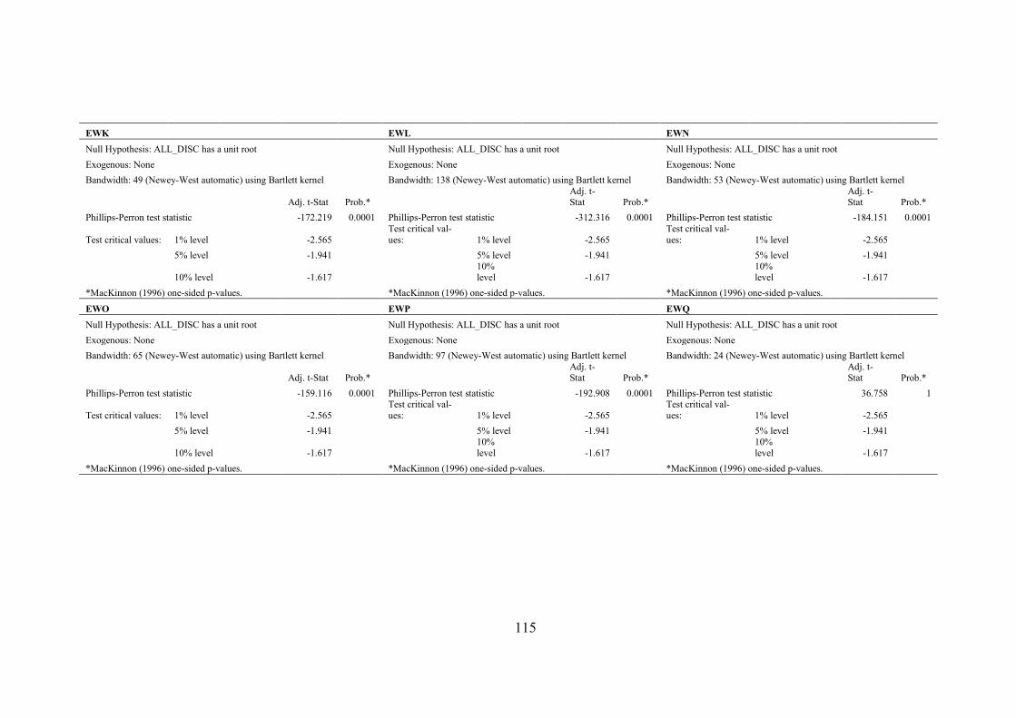
115

EWK EWL EWN Null Hypothesis: ALL_DISC has a unit root Null Hypothesis: ALL_DISC has a unit root Null Hypothesis: ALL_DISC has a unit root Exogenous: None Exogenous: None Exogenous: None Bandwidth: 49 (Newey-West automatic) using Bartlett kernel Bandwidth: 138 (Newey-West automatic) using Bartlett kernel Bandwidth: 53 (Newey-West automatic) using Bartlett kernel


Adj. t-Stat Prob.*





10% level -1.617 10% level -1.617

10% level -1.617


EWO EWP EWQ Null Hypothesis: ALL_DISC has a unit root Null Hypothesis: ALL_DISC has a unit root Null Hypothesis: ALL_DISC has a unit root Exogenous: None Exogenous: None Exogenous: None Bandwidth: 65 (Newey-West automatic) using Bartlett kernel Bandwidth: 97 (Newey-West automatic) using Bartlett kernel Bandwidth: 24 (Newey-West automatic) using Bartlett kernel


Adj. t-Stat Prob.*

Phillips-Perron test statistic -159.116 0.0001 Phillips-Perron test statistic -192.908 0.0001 Phillips-Perron test statistic 36.758 1




10% level -1.617 10% level -1.617

10% level -1.617


116

EWU Null Hypothesis: ALL_DISC has a unit root Exogenous: None Bandwidth: 127 (Newey-West automatic) using Bartlett kernel

Adj. t-Stat Prob.* Phillips-Perron test statistic -290.572 0.0001 Test critical values: 1% level -2.565

5% level -1.941 10% level -1.617


Appendix Table 12: Phillips-Perron Test Results for Synchronous ETPs - Jan 2006 to Jul 2014 - Aggregated Data

IVV EWC EWW Null Hypothesis: ALL_DISC has a unit root Null Hypothesis: ALL_DISC has a unit root Null Hypothesis: ALL_DISC has a unit root Exogenous: None Exogenous: None Exogenous: None Bandwidth: 153 (Newey-West automatic) using Bartlett kernel Bandwidth: 165 (Newey-West automatic) using Bartlett kernel Bandwidth: 134 (Newey-West automatic) using Bartlett kernel

Adj. t-Stat Prob.* Adj. t-Stat Prob.* Adj. t-Stat Prob.* Phillips-Perron test statistic -343.048 0.0001 Phillips-Perron test statistic -317.528 0.0001 Phillips-Perron test statistic -355.150 0.0001 Test critical values: 1% level -2.565 Test critical values: 1% level -2.565 Test critical values: 1% level -2.565



117

EWZ Null Hypothesis: ALL_DISC has a unit root

Exogenous: None Bandwidth: 126 (Newey-West automatic) using Bartlett kernel

Adj. t-Stat Prob.* Phillips-Perron test statistic

-338.188 0.0001


-2.565

5% level

-1.941

10% level

-1.617 *MacKinnon (1996) one-sided p-values.

B.3 KPSS Test Statistics

Appendix Table 13: KPSS Test Results for Non-Synchronous ETPs - Jan 2006 to Jul 2014 - Aggregated Data

EWA

EWH

EWJ Null Hypothesis: ALL_DISC is stationary

Null Hypothesis: ALL_DISC is stationary

Null Hypothesis: ALL_DISC is stationary

Exogenous: Constant

Exogenous: Constant

Exogenous: Constant Bandwidth: 151 (Newey-West automatic) using Bartlett kernel Bandwidth: 143 (Newey-West automatic) using Bartlett kernel Bandwidth: 161 (Newey-West automatic) using Bartlett kernel

LM-Stat.

LM-Stat.

LM-Stat.

Kwiatkowski-Phillips-Schmidt-Shin test statistic 2.986 Kwiatkowski-Phillips-Schmidt-Shin test statistic 4.441 Kwiatkowski-Phillips-Schmidt-Shin test statistic 2.443 Asymptotic critical values*: 1% level

0.739 Asymptotic critical values*: 1% level

0.739 Asymptotic critical values*: 1% level

0.739

5% level

0.463

5% level

0.463

5% level

0.463

10% level

0.347

10% level

0.347

10% level

0.347

*Kwiatkowski-Phillips-Schmidt-Shin (1992, Table 1) *Kwiatkowski-Phillips-Schmidt-Shin (1992, Table 1) *Kwiatkowski-Phillips-Schmidt-Shin (1992, Table 1)

118

EWM EWS EWT Null Hypothesis: ALL_DISC is stationary Null Hypothesis: ALL_DISC is stationary Null Hypothesis: ALL_DISC is stationary Exogenous: Constant Exogenous: Constant Exogenous: Constant Bandwidth: 86 (Newey-West automatic) using Bartlett kernel Bandwidth: 83 (Newey-West automatic) using Bartlett kernel Bandwidth: 149 (Newey-West automatic) using Bartlett kernel

LM-Stat. LM-Stat. LM-Stat. Kwiatkowski-Phillips-Schmidt-Shin test statistic 5.094 Kwiatkowski-Phillips-Schmidt-Shin test statistic 4.512 Kwiatkowski-Phillips-Schmidt-Shin test statistic 4.150 Asymptotic critical values*: 1% level 0.739 Asymptotic critical values*: 1% level 0.739 Asymptotic critical values*: 1% level 0.739

5% level 0.463 5% level 0.463 5% level 0.463 10% level 0.347 10% level 0.347 10% level 0.347


EWY Null Hypothesis: ALL_DISC is stationary Exogenous: Constant Bandwidth: 148 (Newey-West automatic) using Bartlett kernel

LM-Stat. Kwiatkowski-Phillips-Schmidt-Shin test statistic 3.967 Asymptotic critical values*: 1% level

0.739

5% level 0.463 10% level 0.347

*Kwiatkowski-Phillips-Schmidt-Shin (1992, Table 1)

119

Appendix Table 14: KPSS Test Results for Partially Synchronous ETPs - Jan 2006 to Jul 2014 - Aggregated Data

EWD EWG EWI Null Hypothesis: ALL_DISC is stationary Null Hypothesis: ALL_DISC is stationary Null Hypothesis: ALL_DISC is stationary Exogenous: Constant Exogenous: Constant Exogenous: Constant Bandwidth: 115 (Newey-West automatic) using Bartlett kernel Bandwidth: 104 (Newey-West automatic) using Bartlett kernel Bandwidth: 129 (Newey-West automatic) using Bartlett kernel




EWK EWL EWN Null Hypothesis: ALL_DISC is stationary Null Hypothesis: ALL_DISC is stationary Null Hypothesis: ALL_DISC is stationary Exogenous: Constant Exogenous: Constant Exogenous: Constant Bandwidth: 55 (Newey-West automatic) using Bartlett kernel Bandwidth: 147 (Newey-West automatic) using Bartlett kernel Bandwidth: 62 (Newey-West automatic) using Bartlett kernel




EWO EWP EWQ Null Hypothesis: ALL_DISC is stationary Null Hypothesis: ALL_DISC is stationary Null Hypothesis: ALL_DISC is stationary Exogenous: Constant Exogenous: Constant Exogenous: Constant Bandwidth: 75 (Newey-West automatic) using Bartlett kernel Bandwidth: 93 (Newey-West automatic) using Bartlett kernel Bandwidth: 103 (Newey-West automatic) using Bartlett kernel




120

EWU Null Hypothesis: ALL_DISC is stationary Exogenous: Constant Bandwidth: 104 (Newey-West automatic) using Bartlett kernel


0.739

5% level 0.463 10% level 0.347


121

Appendix Table 15: KPSS Test Results for Synchronous ETPs - Jan 2006 to Jul 2014 - Aggregated Data

IVV EWC EWW Null Hypothesis: ALL_DISC is stationary Null Hypothesis: ALL_DISC is stationary Null Hypothesis: ALL_DISC is stationary Exogenous: Constant Exogenous: Constant Exogenous: Constant Bandwidth: 158 (Newey-West automatic) using Bartlett kernel Bandwidth: 84 (Newey-West automatic) using Bartlett kernel Bandwidth: 136 (Newey-West automatic) using Bartlett kernel




EWZ Null Hypothesis: ALL_DISC is stationary Exogenous: Constant Bandwidth: 127 (Newey-West automatic) using Bartlett kernel


0.739

5% level 0.463 10% level 0.347


122

Appendix CAppendix Table 16: Descriptive Statistics for Partially Synchronous ETPs - 11:00am to 11:15am

Sweden Germany Italy Belgium Switzerland Netherlands Austria Spain France United Kingdom

Ticker EWD EWG EWI EWK EWL EWN EWO EWP EWQ EWU Mean -13.18 -12.96 -13.25 -13.89 -13.70 -14.05 -13.75 -13.20 -13.43 -13.15 Median -13.01 -12.94 -13.08 -13.60 -13.56 -13.82 -13.47 -13.05 -13.27 -13.14 Maximum -8.12 -8.19 -8.47 -7.05 -7.84 -7.13 -8.16 -8.26 -8.08 -8.68 Minimum -27.20 -19.78 -27.68 -27.12 -27.11 -27.12 -27.62 -28.51 -27.65 -25.42 Std. Dev. 1.65 1.30 1.75 2.26 1.77 2.04 2.07 1.60 1.65 1.35 Skewness -1.03 -0.08 -1.26 -1.76 -1.67 -1.52 -1.91 -1.47 -1.17 -0.47 Kurtosis 7.14 4.08 8.88 10.42 13.01 9.94 11.78 11.37 8.85 6.83 Observations 2 049 2 143 1 832 1 387 2 057 1 655 1 734 2 028 1 965 2 134

Appendix Table 17: Results of Wilcoxon Signed Rank Test for Partially Synchronous ETPs - 11:00am to 11:15am compared with 11:15am to 11:30am

Hypothesis Testing for EWD Hypothesis Testing for EWG Hypothesis Testing for EWI Included observations: 2036 Included observations: 2141 Included observations: 1829 Test of Hypothesis: Median = -13.00506 Test of Hypothesis: Median = -12.93803 Test of Hypothesis: Median = -13.08127 Sample Median = -13.18799 Sample Median = -13.13627 Sample Median = -13.19373 Method Value Probability Method Value Probability Method Value Probability Wilcoxon signed rank 6.658802 0.00% Wilcoxon signed rank 6.426959 0.00% Wilcoxon signed rank 5.736851 0.00% Median Test Summary Median Test Summary Median Test Summary Category Count Mean Rank Category Count Mean Rank Category Count Mean Rank Obs > -13.00506 908 947.3293 46.53% Obs > -12.93803 926 1039.571 48.56% Obs > -13.08127 852 830.0164 45.38% Obs < -13.00506 1128 1075.79 52.84% Obs < -12.93803 1215 1094.953 51.14% Obs < -13.08127 977 989.1105 54.08% Obs = -13.00506 0 Obs = -12.93803 0 Obs = -13.08127 0

123

Hypothesis Testing for EWK

Hypothesis Testing for EWL Included observations: 1383

Included observations: 2055

Test of Hypothesis: Median = -13.59708 Test of Hypothesis: Median = -13.55531 Sample Median = -13.52582

Sample Median = -13.66719

Method

Value Probability Method

Value Probability Wilcoxon signed rank 1.080666 0.280 Wilcoxon signed rank 3.778651 0.02% Median Test Summary

Median Test Summary

Category Count Mean Rank Category Count Mean Rank Obs > -13.59708 710 651.3577 47.10% Obs > -13.55531 975 979.0933 47.64% Obs < -13.59708 673 734.8767 53.14% Obs < -13.55531 1080 1072.152 52.17% Obs = -13.59708 0

Obs = -13.55531 0

Hypothesis Testing for EWN

Hypothesis Testing for EWO

Hypothesis Testing for EWP Included observations: 1583



Test of Hypothesis: Median = -13.81728 Test of Hypothesis: Median = -13.47002 Test of Hypothesis: Median = -13.04630 Sample Median = -13.92976



Method



Value Probability Wilcoxon signed rank 4.730553 0.00% Wilcoxon signed rank 2.476798 1.33% Wilcoxon signed rank 6.594533 0.00% Median Test Summary

Median Test Summary

Median Test Summary

Category Count Mean Rank Category Count Mean Rank Category Count Mean Rank Obs > -13.81728 735 735.8068 46.48% Obs > -13.47002 866 811.7125 46.73% Obs > -13.04630 907 947.3142 46.60% Obs < -13.81728 848 840.7052 53.11% Obs < -13.47002 871 925.9587 53.31% Obs < -13.04630 1126 1073.132 52.79% Obs = -13.81728 0

Obs = -13.47002 0

Obs = -13.04630 0

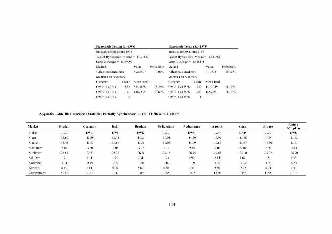
124

Hypothesis Testing for EWQ Hypothesis Testing for EWU Included observations: 1976 Included observations: 2136 Test of Hypothesis: Median = -13.27437 Test of Hypothesis: Median = -13.13868 Sample Median = -13.49999 Sample Median = -13.16115 Method Value Probability Method Value Probability Wilcoxon signed rank 8.213997 0.00% Wilcoxon signed rank 0.199331 84.20% Median Test Summary Median Test Summary Category Count Mean Rank Category Count Mean Rank Obs > -13.27437 859 894.3888 45.26% Obs > -13.13868 1052 1079.349 50.53% Obs < -13.27437 1117 1060.874 53.69% Obs < -13.13868 1084 1057.971 49.53% Obs = -13.27437 0 Obs = -13.13868 0

Appendix Table 18: Descriptive Statistics Partially Synchronous ETPs - 11:30am to 11:45am

Market Sweden Germany Italy Belgium Switzerland Netherlands Austria Spain France United Kingdom

Ticker EWD EWG EWI EWK EWL EWN EWO EWP EWQ EWU Mean -13.60 -13.59 -13.74 -14.13 -14.04 -14.39 -13.91 -13.68 -14.09 -13.63 Median -13.45 -13.63 -13.56 -13.78 -13.98 -14.19 -13.66 -13.57 -13.92 -13.61 Maximum -8.64 -8.20 -9.05 -8.07 -9.11 -9.15 -7.04 -9.16 -8.99 -7.10 Minimum -27.61 -22.57 -25.32 -26.88 -27.12 -26.95 -27.65 -28.10 -27.77 -26.70 Std. Dev. 1.71 1.41 1.75 2.31 1.73 1.99 2.14 1.67 1.81 1.49 Skewness -1.11 -0.15 -0.79 -1.66 -0.60 -1.09 -1.49 -1.93 -1.23 -0.85 Kurtosis 8.44 4.61 5.06 8.69 5.26 7.46 9.56 15.25 8.94 9.41 Observations 2 019 2 142 1 747 1 303 1 999 1 525 1 670 1 993 1 919 2 112

125

Appendix Table 19: Results of Wilcoxon Signed Rank Test for Partially Synchronous ETPs - 11:30am to 11:45am compared with 11:45am to 12:00pm

Hypothesis Testing for EWD Hypothesis Testing for EWG Hypothesis Testing for EWI Included observations: 2017 Included observations: 2143 Included observations: 1805 Test of Hypothesis: Median = -13.45105 Test of Hypothesis: Median = -13.62830 Test of Hypothesis: Median = -13.56348 Sample Median = -13.12493 Sample Median = -13.24529 Sample Median = -13.06859 Method Value Probability Method Value Probability Method Value Probability Wilcoxon signed rank 6.33260989 0.00% Wilcoxon signed rank 14.1648363 0.00% Wilcoxon signed rank 9.91469297 0.00% Median Test Summary Median Test Summary Median Test Summary Category Count Mean Rank Category Count Mean Rank Category Count Mean Rank Obs > -13.45105 1177 1005.29737 49.84% Obs > -13.62830 1335 1164.37678 54.33% Obs > -13.56348 1124 920.403915 50.99% Obs < -13.45105 840 1014.1881 50.28% Obs < -13.62830 808 919.372525 42.90% Obs < -13.56348 681 874.274596 48.44% Obs = -13.45105 0 Obs = -13.62830 0 Obs = -13.56348 0

Hypothesis Testing for EWK Hypothesis Testing for EWL Hypothesis Testing for EWN Included observations: 1357 Included observations: 2037 Included observations: 1546 Test of Hypothesis: Median = -13.78441 Test of Hypothesis: Median = -13.97745 Test of Hypothesis: Median = -14.18538 Sample Median = -13.41681 Sample Median = -13.50323 Sample Median = -13.73076 Method Value Probability Method Value Probability Method Value Probability Wilcoxon signed rank 5.66662 0.00% Wilcoxon signed rank 13.8678 0.00% Wilcoxon signed rank 7.780318 0.00% Median Test Summary Median Test Summary Median Test Summary

Category Count Mean Rank Category Count Mean Rank Category Count Mean Rank Obs > -13.78441 787 689.3506 50.80% Obs > -13.9774 1295 1085.741 53.30% Obs > -14.18538 958 766.7119 49.59% Obs < -13.78441 570 664.7087 48.98% Obs < -13.9774 742 902.517 44.31% Obs < -14.18538 588 784.559524 50.75% Obs = -13.78441 0 Obs = -13.9774 0 Obs = -14.18538 0

126

Hypothesis Testing for EWO Hypothesis Testing for EWP Hypothesis Testing for EWQ Included observations: 1755 Included observations: 2029 Included observations: 1949 Test of Hypothesis: Median = -13.65772 Test of Hypothesis: Median = -13.57462 Test of Hypothesis: Median = -13.92304 Sample Median = -13.13770 Sample Median = -12.96897 Sample Median = -13.40151 Method Value Probability Method Value Probability Method Value Probability Wilcoxon signed rank 9.47547 0.00% Wilcoxon signed rank 16.5382 0.00% Wilcoxon signed rank 14.0855 0.00% Median Test Summary Median Test Summary Median Test Summary Category Count Mean Rank Category Count Mean Rank Category Count Mean Rank Obs > -13.65772 1095 887.3406 50.56% Obs > -13.57462 1371 1069.450 52.71% Obs > -13.92304 1282 1014.148 52.03% Obs < -13.65772 660 862.5030 49.15% Obs < -13.57462 658 901.5486 44.43% Obs < -13.92304 667 899.7556 46.16% Obs = -13.65772 0 Obs = -13.57462 0 Obs = -13.92304 0

Hypothesis Testing for EWP Hypothesis Testing for EWQ Hypothesis Testing for EWU Included observations: 2029 Included observations: 1949 Included observations: 2117 Test of Hypothesis: Median = -13.57462 Test of Hypothesis: Median = -13.92304 Test of Hypothesis: Median = -13.61175 Sample Median = -12.96897 Sample Median = -13.40151 Sample Median = -13.12926 Method Value Probability Method Value Probability Method Value Probability Wilcoxon signed rank 16.5382 0.00% Wilcoxon signed rank 14.0856 0.00% Wilcoxon signed rank 17.2349 0.00% Median Test Summary Median Test Summary Median Test Summary Category Count Mean Rank Category Count Mean Rank Category Count Mean Rank Obs > -13.57462 1371 1069.45 52.71% Obs > -13.92304 1282 1014.15 52.03% Obs > -13.61175 1398 1148.6 54.26% Obs < -13.57462 658 901.549 44.43% Obs < -13.92304 667 899.756 46.16% Obs < -13.61175 719 884.787 41.79% Obs = -13.57462 0 Obs = -13.92304 0 Obs = -13.61175 0

Analysis of non-synchronous trading effects on the pricing ...

Documents

Transcript of Analysis of non-synchronous trading effects on the pricing ...