
Analysis of Missing Data with Random Forests - uni · PDF fileAnalysis of Missing Data with...
168
Analysis of Missing Data with Random Forests Alexander Hapfelmeier M¨ unchen 2012
Transcript of Analysis of Missing Data with Random Forests - uni · PDF fileAnalysis of Missing Data with...

Analysis of Missing Data withRandom Forests
Alexander Hapfelmeier
Munchen 2012

Analysis of Missing Data withRandom Forests
Alexander Hapfelmeier
Dissertation
zur Erlangung des akademischen Grades
eines Doktors der Naturwissenschaften
am Institut fur Statistik
an der Fakultat fur Mathematik, Informatik und Statistik
der Ludwig–Maximilians–Universitat Munchen
vorgelegt von
Alexander Hapfelmeier
Munchen, den 09.05.2012

Erstgutachter: Prof. Dr. Kurt Ulm
Zweitgutachter: Prof. Dr. Torsten Hothorn
Externer Gutachter: Prof. PhD Adele Cutler
Tag der Disputation: 12.10.2012

v
To my family

vi

Acknowledgement
I owe my deepest gratitude to Prof. Dr. Kurt Ulm who made this thesis possible andsupported me in any possible way. Likewise, I am heartily thankful to Prof. Dr. TorstenHothorn and Prof. Dr. Carolin Strobl for their supervision and support. I also would liketo thank all of my colleagues for their help and constructive discussions.

viii

Contents
Summary xvii
Zusammenfassung xviii
Introduction xx
Scope of Work xxiii
1 Recursive Partitioning 11.1 Classification and Regression Trees . . . . . . . . . . . . . . . . . . . . . . 1
1.1.1 Rationale . . . . . . . . . . . . . . . . . . . . . . . . . . . . . . . . 11.1.2 The CART Algorithm . . . . . . . . . . . . . . . . . . . . . . . . . 21.1.3 Conditional Inference Trees . . . . . . . . . . . . . . . . . . . . . . 41.1.4 Surrogate Splits . . . . . . . . . . . . . . . . . . . . . . . . . . . . . 6
1.2 Random Forests . . . . . . . . . . . . . . . . . . . . . . . . . . . . . . . . . 81.2.1 Rationale and Definition . . . . . . . . . . . . . . . . . . . . . . . . 81.2.2 Importance Measures . . . . . . . . . . . . . . . . . . . . . . . . . . 9
1.3 Statistical Software . . . . . . . . . . . . . . . . . . . . . . . . . . . . . . . 14
2 Predictive Accuracy for Data with Missing Values 172.1 Research Motivation and Contribution . . . . . . . . . . . . . . . . . . . . 172.2 Discussion of Related Publications . . . . . . . . . . . . . . . . . . . . . . . 182.3 Missing Data . . . . . . . . . . . . . . . . . . . . . . . . . . . . . . . . . . 20
2.3.1 Missing Data Generating Processes . . . . . . . . . . . . . . . . . . 202.3.2 Multivariate Imputation by Chained Equations . . . . . . . . . . . 21
2.4 Studies . . . . . . . . . . . . . . . . . . . . . . . . . . . . . . . . . . . . . . 242.4.1 Simulation Studies . . . . . . . . . . . . . . . . . . . . . . . . . . . 252.4.2 Empirical Evaluation . . . . . . . . . . . . . . . . . . . . . . . . . . 272.4.3 Implementation . . . . . . . . . . . . . . . . . . . . . . . . . . . . . 29
2.5 Results . . . . . . . . . . . . . . . . . . . . . . . . . . . . . . . . . . . . . . 302.5.1 Simulation Studies . . . . . . . . . . . . . . . . . . . . . . . . . . . 302.5.2 Empirical Evaluation . . . . . . . . . . . . . . . . . . . . . . . . . . 31
2.6 Discussion and Conclusion . . . . . . . . . . . . . . . . . . . . . . . . . . . 34

x CONTENTS
3 A new Variable Importance Measure for Missing Data 393.1 Research Motivation and Contribution . . . . . . . . . . . . . . . . . . . . 393.2 New Proposal . . . . . . . . . . . . . . . . . . . . . . . . . . . . . . . . . . 40
3.2.1 Definition . . . . . . . . . . . . . . . . . . . . . . . . . . . . . . . . 403.2.2 Requirements . . . . . . . . . . . . . . . . . . . . . . . . . . . . . . 41
3.3 Studies . . . . . . . . . . . . . . . . . . . . . . . . . . . . . . . . . . . . . . 423.3.1 Simulation Studies . . . . . . . . . . . . . . . . . . . . . . . . . . . 423.3.2 Empirical Evaluation . . . . . . . . . . . . . . . . . . . . . . . . . . 453.3.3 Implementation . . . . . . . . . . . . . . . . . . . . . . . . . . . . . 45
3.4 Results . . . . . . . . . . . . . . . . . . . . . . . . . . . . . . . . . . . . . . 463.4.1 Simulation Studies . . . . . . . . . . . . . . . . . . . . . . . . . . . 463.4.2 Empirical Evaluation . . . . . . . . . . . . . . . . . . . . . . . . . . 50
3.5 Discussion and Conclusion . . . . . . . . . . . . . . . . . . . . . . . . . . . 54
4 Variable Importance with Missing Data 574.1 Research Motivation and Contribution . . . . . . . . . . . . . . . . . . . . 574.2 Simulation Studies . . . . . . . . . . . . . . . . . . . . . . . . . . . . . . . 584.3 Results . . . . . . . . . . . . . . . . . . . . . . . . . . . . . . . . . . . . . . 594.4 Conclusion . . . . . . . . . . . . . . . . . . . . . . . . . . . . . . . . . . . . 62
5 A new Variable Selection Method 655.1 Research Motivation and Contribution . . . . . . . . . . . . . . . . . . . . 655.2 Variable Selection . . . . . . . . . . . . . . . . . . . . . . . . . . . . . . . . 66
5.2.1 Performance-based Approaches . . . . . . . . . . . . . . . . . . . . 675.2.2 Test-based Approaches . . . . . . . . . . . . . . . . . . . . . . . . . 705.2.3 New Method . . . . . . . . . . . . . . . . . . . . . . . . . . . . . . 71
5.3 Studies . . . . . . . . . . . . . . . . . . . . . . . . . . . . . . . . . . . . . . 745.3.1 Simulation Studies . . . . . . . . . . . . . . . . . . . . . . . . . . . 745.3.2 Empirical Evaluation . . . . . . . . . . . . . . . . . . . . . . . . . . 775.3.3 Implementation . . . . . . . . . . . . . . . . . . . . . . . . . . . . . 785.3.4 Settings of Variable Selection Approaches . . . . . . . . . . . . . . . 79
5.4 Results . . . . . . . . . . . . . . . . . . . . . . . . . . . . . . . . . . . . . . 795.4.1 Simulation Studies . . . . . . . . . . . . . . . . . . . . . . . . . . . 795.4.2 Empirical Evaluation . . . . . . . . . . . . . . . . . . . . . . . . . . 84
5.5 Discussion and Conclusion . . . . . . . . . . . . . . . . . . . . . . . . . . . 84
6 Variable Selection with Missing Data 876.1 Research Motivation and Contribution . . . . . . . . . . . . . . . . . . . . 876.2 Simulation Studies . . . . . . . . . . . . . . . . . . . . . . . . . . . . . . . 886.3 Results . . . . . . . . . . . . . . . . . . . . . . . . . . . . . . . . . . . . . . 896.4 Conclusion . . . . . . . . . . . . . . . . . . . . . . . . . . . . . . . . . . . . 92
Outlook 94

Contents xi
A Supplementary Material 97A.1 Chapter 2 . . . . . . . . . . . . . . . . . . . . . . . . . . . . . . . . . . . . 97
A.1.1 Simulation Studies . . . . . . . . . . . . . . . . . . . . . . . . . . . 97A.1.2 Empirical Evaluation . . . . . . . . . . . . . . . . . . . . . . . . . . 99
A.2 Chapter 3 . . . . . . . . . . . . . . . . . . . . . . . . . . . . . . . . . . . . 99A.3 Chapter 4 . . . . . . . . . . . . . . . . . . . . . . . . . . . . . . . . . . . . 103A.4 Chapter 5 . . . . . . . . . . . . . . . . . . . . . . . . . . . . . . . . . . . . 104
A.4.1 Simulation Studies . . . . . . . . . . . . . . . . . . . . . . . . . . . 104A.4.2 Empirical Evaluation . . . . . . . . . . . . . . . . . . . . . . . . . . 110
A.5 Chapter 6 . . . . . . . . . . . . . . . . . . . . . . . . . . . . . . . . . . . . 112
B R-Code 113B.1 Chapter 1 . . . . . . . . . . . . . . . . . . . . . . . . . . . . . . . . . . . . 114B.2 Chapter 2 . . . . . . . . . . . . . . . . . . . . . . . . . . . . . . . . . . . . 115
B.2.1 Simulation Studies . . . . . . . . . . . . . . . . . . . . . . . . . . . 115B.2.2 Empirical Evaluation . . . . . . . . . . . . . . . . . . . . . . . . . . 117
B.3 Chapter 3 . . . . . . . . . . . . . . . . . . . . . . . . . . . . . . . . . . . . 118B.3.1 Simulation Studies . . . . . . . . . . . . . . . . . . . . . . . . . . . 118B.3.2 Empirical Evaluation . . . . . . . . . . . . . . . . . . . . . . . . . . 119
B.4 Chapter 4 . . . . . . . . . . . . . . . . . . . . . . . . . . . . . . . . . . . . 120B.5 Chapter 5 . . . . . . . . . . . . . . . . . . . . . . . . . . . . . . . . . . . . 122
B.5.1 Functions to perform Variable Selection . . . . . . . . . . . . . . . . 122B.5.2 Simulation Studies . . . . . . . . . . . . . . . . . . . . . . . . . . . 127B.5.3 Empirical Evaluation . . . . . . . . . . . . . . . . . . . . . . . . . . 131
B.6 Chapter 6 . . . . . . . . . . . . . . . . . . . . . . . . . . . . . . . . . . . . 132

xii Contents

List of Figures
1.1 Regression tree and corresponding segmentation of variable space . . . . . 21.2 Visualization of the 1 s.e. rule: plot of tree sizes against cross-validated error 41.3 Example of a conditional inference tree . . . . . . . . . . . . . . . . . . . . 51.4 Schematic view of the surrogate split conception . . . . . . . . . . . . . . . 71.5 Approximation of functional relations by ensembles of trees . . . . . . . . . 81.6 Single trees of a Random Forest . . . . . . . . . . . . . . . . . . . . . . . . 101.7 Selections frequencies of predictors (air quality example) . . . . . . . . . . 111.8 Permutation accuracy importance (air quality example) . . . . . . . . . . . 15
2.1 MSE values observed for the simulation studies . . . . . . . . . . . . . . . 332.2 MSE values observed for the application studies . . . . . . . . . . . . . . . 35
3.1 Comparison of the original permutation importance and the new approach 473.2 Variable importance for an increasing number of missing values . . . . . . 473.3 Variable importance for an increasing correlation strength . . . . . . . . . 483.4 Variable importances and selection frequencies . . . . . . . . . . . . . . . . 493.5 Variable importances and selection frequencies of isolated blocks of variables 493.6 Variable importances of influential and non-influential variables . . . . . . 503.7 General view of all results for the MAR(rank) scheme . . . . . . . . . . . . 513.8 Summary of results for all MCAR, MAR and MNAR schemes . . . . . . . 523.9 Variable importances for the Pima Indians and Mammal Sleep Data . . . . 533.10 Variable importances for the additional simulation study . . . . . . . . . . 55
4.1 Median variable importance observed for the new importance measure . . . 604.2 Median variable importance observed for the complete case analysis . . . . 614.3 Median variable importance observed for the imputed data . . . . . . . . . 624.4 MSE observed for the classification problem . . . . . . . . . . . . . . . . . 63
5.1 Power comparison example . . . . . . . . . . . . . . . . . . . . . . . . . . . 745.2 Selection frequencies (study II) . . . . . . . . . . . . . . . . . . . . . . . . 825.3 Selection frequencies and MSE (study III) . . . . . . . . . . . . . . . . . . 85
6.1 Variable selection frequencies observed for the new importance measure . . 906.2 Variable selection frequencies observed for the complete case analysis . . . 91

xiv Figures
6.3 Variable selection frequencies observed for the imputed data . . . . . . . . 926.4 MSE observed for the independent test data . . . . . . . . . . . . . . . . . 93
A.1 Chapter 3: Variable importance of variables with missing values . . . . . . 100A.2 Chapter 3: Variable importance of correlated variables . . . . . . . . . . . 101A.3 Chapter 3: General view of the MAR(rank) scheme (classification problem) 102A.4 Chapter 4: Median variable importance (regression problem) . . . . . . . . 103A.5 Chapter 4: MSE (regression problem) . . . . . . . . . . . . . . . . . . . . . 104A.6 Chapter 5: Selection frequencies (study II) . . . . . . . . . . . . . . . . . . 107A.7 Chapter 5: Selection frequencies (study II; regression problem) . . . . . . . 108A.8 Chapter 5: Selection frequencies and MSE (study III) . . . . . . . . . . . . 109A.9 Chapter 5: Selection frequencies and MSE (study III; regression problem) . 110A.10 Chapter 6: Variable selection frequencies and MSE (regression problem) . . 112

List of Tables
1.1 Split rules and descriptive statistics of final nodes (air quality example) . . 21.2 Summary of functions used to perform recursive partitioning . . . . . . . . 15
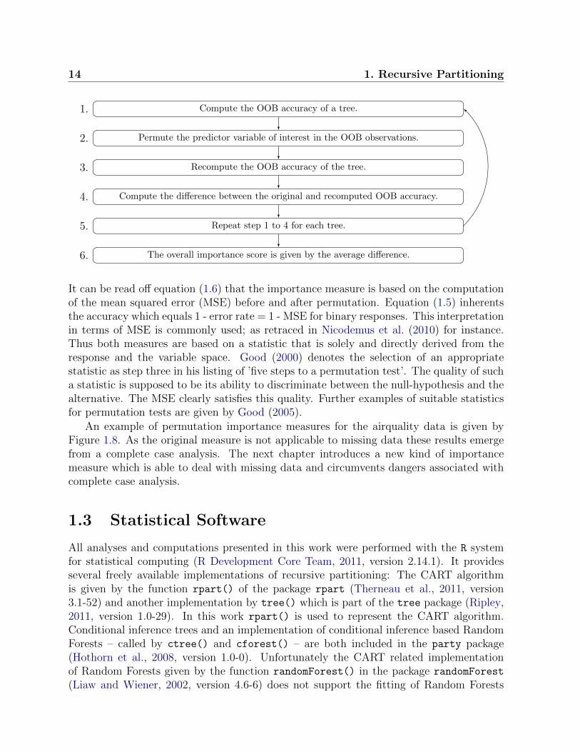
2.1 Description of data used in the simulation studies. . . . . . . . . . . . . . . 262.2 Description of data used in the application studies. . . . . . . . . . . . . . 302.3 Summary of results for the simulation studies. . . . . . . . . . . . . . . . . 322.4 Summary of results for the application studies. . . . . . . . . . . . . . . . . 34
3.1 Variables involved in the missing data generating process (chapter 3) . . . 44
4.1 Variables involved in the missing data generating process (chapter 4) . . . 59
5.1 Characteristics of data used in the application studies . . . . . . . . . . . . 785.2 Summary of variable selection methods, labels and specific settings . . . . 805.3 TWER and FWER of the classification problem (study I) . . . . . . . . . . 815.4 Bootstrap, resubstitution and .632 MSE estimates (empirical evaluation) . 86
6.1 Variables involved in the missing data generating process (chapter 6) . . . 89
A.1 Chapter 2: Detailed listing of results for the simulation studies. . . . . . . 97A.2 Chapter 2: Detailed listing of results for the application studies. . . . . . . 99A.3 Chapter 5: TWER and FWER (study I; regression problem) . . . . . . . . 105A.4 Chapter 5: Variable selection frequencies (empirical evaluation) . . . . . . 111

xvi Tables

Summary
Random Forests are widely used for data prediction and interpretation purposes. Theyshow many appealing characteristics, such as the ability to deal with high dimensional data,complex interactions and correlations. Furthermore, missing values can easily be processedby the built-in procedure of surrogate splits. However, there is only little knowledge aboutthe properties of recursive partitioning in missing data situations. Therefore, extensivesimulation studies and empirical evaluations have been conducted to gain deeper insight.In addition, new methods have been developed to enhance methodology and solve currentissues of data interpretation, prediction and variable selection.
A variable’s relevance in a Random Forest can be assessed by means of importancemeasures. Unfortunately, existing methods cannot be applied when the data contain miss-ing values. Thus, one of the most appreciated properties of Random Forests – its abilityto handle missing values – gets lost for the computation of such measures. This workpresents a new approach that is designed to deal with missing values in an intuitive andstraightforward way, yet retains widely appreciated qualities of existing methods. Resultsindicate that it meets sensible requirements and shows good variable ranking properties.
Random Forests provide variable selection that is usually based on importance mea-sures. An extensive review of corresponding literature led to the development of a newapproach that is based on a profound theoretical framework and meets important statis-tical properties. A comparison to another eight popular methods showed that it controlsthe test-wise and family-wise error rate, provides a higher power to distinguish relevantfrom non-relevant variables and leads to models located among the best performing ones.
Alternative ways to handle missing values are the application of imputation methodsand complete case analysis. Yet it is unknown to what extent these approaches are ableto provide sensible variable rankings and meaningful variable selections. Investigationsshowed that complete case analysis leads to inaccurate variable selection as it may in-appropriately penalize the importance of fully observed variables. By contrast, the newimportance measure decreases for variables with missing values and therefore causes se-lections that accurately reflect the information given in actual data situations. Multipleimputation leads to an assessment of a variable’s importance and to selection frequenciesthat would be expected for data that was completely observed. In several performanceevaluations the best prediction accuracy emerged from multiple imputation, closely fol-lowed by the application of surrogate splits. Complete case analysis clearly performedworst.

xviii Zusammenfassung

Zusammenfassung
Random Forests werden in vielen wissenschaftlichen Bereichen fur die Datenanalyse undals Pradiktionsmodell verwendet. Sie besitzen zahlreiche vorteilhafte Fahigkeiten wiemit hochdimensionalen Daten sowie komplexen Interaktions- und Korrelationsstrukturenumgehen zu konnen. Bislang ist jedoch wenig uber ihre Eigenschaften in Datensituatio-nen mit fehlenden Werten bekannt, obgleich sich diese sehr einfach mit Hilfe sogenannter“surrogate splits” behandeln lassen. In dieser Arbeit wurden umfangreiche Simulationsund Evaluationsstudien durchgefuhrt um entsprechende Einsichten zu gewinnen. NeueVerfahren wurden entwickelt um aktuelle Problemstellungen zu losen.
Durch Wichtigkeitsmaße kann die Relevanz einer Variablen in Random Forests beurteiltwerden. Unglucklicherweise lassen sie sich bislang nicht berechnen wenn fehlende Wertein den Daten vorhanden sind. In dieser Arbeit wird durch die Einfuhrung einer neuenMethode eine Losung fur dieses Problem prasentiert. Sie orientiert sich dabei an bereitsexistierenden Maßen und behalt somit beliebte Eigenschaften bei. Es zeigte sich, dass dasneue Maß zuvor gestellte Anforderungen erfullt und gewunschte Eigenschaften aufweist.
Die Moglichkeit der Variablenselektion basierend auf Wichtigkeitsmaßen ist eine zusatz-liche Starke von Random Forests. Eine ausfuhrliche Literaturrecherche fuhrte zu derIdee einer neuen Methode, die basierend of profunden wahrscheinlichkeitstheoretischenGrundlagen wichtige statistische Eigenschaften erfullt. Im Vergleich mit acht etabliertenAlgorithmen erwies sie sich als geeignet die vergleichsbezogenen und versuchsbezogenenIrrtumswahrscheinlichkeiten zu kontrollieren und zeigte eine hohe Trennscharfe fur die Un-terscheidung von relevanten und nicht relevanten Variablen. Hierauf basierende RandomForests erzielten außerdem hohe Vorhersageguten.
Alternativ lassen sich fehlende Werte durch “complete case” Analysen und Imputa-tion behandeln. Es ist jedoch nicht bekannt inwiefern sich mit diesen Verfahren sinn-volle Wichtigkeitsmaße oder Variablenselektionen berechnen bzw. durchfuhren lassen.Entsprechende Untersuchungen zeigten, dass complete case Analysen zu inadequaten Se-lektionen fuhren, da die Wichtigkeit vollstandig beobachteter Variablen falschlich herabge-wertet werden kann. Das neue Wichtigkeitsmaß sinkt dagegen ausschließlich fur Variablenmit fehlenden Werten und erzeugt somit Selektionen, die tatsachliche Datensituationenwiderspiegeln. Ein Imputationsverfahren fuhrt zu Ergebnissen, die fur vollstandige Datenzu erwarten gewesen waren. In mehreren Bewertungen wurden fur Letzteres auch diebesten Vorhersageguten ermittelt. Die Anwendung von Surrogaten war nur unwesentlichschlechter wobei complete case Analysen deutlich am schlechtesten abschnitten.

xx Introduction

Introduction
Recursive partitioning methods, in particular classification and regression trees and Ran-dom Forests, are popular approaches in statistical data analysis. They are applied fordata prediction and interpretation purposes in many research fields such as social, econo-metric and clinical science. Among others, there are approaches like the famous CARTalgorithm introduced by Breiman et al. (1984), the C4.5 algorithm by Quinlan (1993) andconditional inference trees by Hothorn et al. (2006). A detailed listing of application areasand methodological issues, along with discussions about the historical development andstate-of-the-art, can be found in Strobl et al. (2009). The popularity of trees is rooted inseveral appealing characteristics like their easy applicability and interpretability in both,classification and regression problems. Advantages over common approaches like logisticand linear regression are their ability to implicitly deal with missing values, collinearity,nonlinearity and high dimensional data. Random Forests are able to achieve competitiveor even superior prediction strengths in comparison to well established approaches (i.e.regression, linear discriminant analysis, support vector machines, neural nets etc.). More-over, recursive partitioning is able to handle even complex interaction effects – which is ahighly valued property e.g. for the analysis of gene-gene relations (Lunetta et al., 2004;Cutler et al., 2007; Tang et al., 2009; Nicodemus et al., 2010).
The main focus of this work is put on the performance and applicability of RandomForests and corresponding features – like variable importance measures and variable se-lection – in missing data analysis. Therefore, after a short introduction of methodologyin chapter 1, the predictive accuracy of Random Forests – and single trees – is exploredand compared between the application to data with and without a preliminary imputationof missing values in chapter 2. Several datasets that provide classification and regressionproblems have been used for simulation studies and empirical evaluations. For the former,missing values were induced into fully observed data while for the latter, data were usedthat already contained missing values. Multiple imputation produced variable results whilethe application of surrogates appeared to be a fast and simple way to achieve performanceswhich are only negligibly worse and in many cases even superior.
An important feature of Random Forests is the evaluation of a variable’s relevance bymeans of importance measures. However, existing measures cannot be computed in thepresence of missing values. A straightforward application to such data leads to violations oftheir most basic conceptual principles. A solution to this issue is introduced in chapter 3: Anew approach makes the computation of variable importance measures possible even when

xxii Introduction
there are missing data. Its properties are investigated in an extensive simulation study.Results show that a list of sensible, pre-specified requirements are completely fulfilled. Anapplication to two datasets also shows its practicality in real life situations.
Imputation methods and complete case analysis are two alternative approaches that en-able the computation of importance measures in the presence of missing values. However,it is unknown to what extend these approaches are able to provide a reliable estimate of avariable’s relevance. Therefore, an extensive simulation study was performed in chapter 4to investigate this property for a variety of missing data generating processes. Predictionaccuracy has been explored in accordance with investigations of chapter 2. Findings sug-gest that complete case analysis should not be applied as it may inappropriately penalizevariables that were completely observed. The new importance measure is much more ca-pable of reflecting decreased information exclusively for variables with missing values andshould therefore be used to evaluate actual data situations. By contrast, multiple impu-tation allows for an estimation of importances one would potentially observe in completedata situations.
Importance measures are often used as a basis for variable selection. Many works (e.g.Tang et al., 2009; Yang and Gu, 2009; Rodenburg et al., 2008; Sandri and Zuccolotto,2006; Dıaz-Uriarte and Alvarez de Andres, 2006) show that different approaches have beendeveloped to distinguish relevant from non-relevant variables and to improve predictionaccuracy. An extensive review of the corresponding literature led to the development of anew approach that is based on a more profound theoretical framework and meets importantstatistical properties. A comparison to another eight established selection approaches isgiven in chapter 5. The new proposal is able to outperform these competitors in threesimulation studies and four empirical evaluations with regard to discriminatory power andprediction accuracy of resulting models.
Once again, alternatives are given by complete case analysis and imputation methods.Therefore an extensive simulation study has been conducted in chapter 6 to explore theability of each approach – in combination with the new variable selection method and apopular representative of established approaches – to distinguish relevant from non-relevantvariables. In accordance with chapter 2 and chapter 4 the predictive accuracy of resultingmodels has been investigated, too. Findings suggest that complete case analysis shouldnot be applied as it leads to inaccurate variable selection. Multiple imputation is a goodmeans to select variables that would be of relevance in fully observed data. By contrast,the application of the new importance measure caused a selection of variables that reflectsthe actual data situation, i.e. that takes the occurrence of missing values into account.
In conclusion, this work presents extensive investigations of Random Forests for theanalysis of data with missing values. Important aspects like predictive accuracy, vari-able importance and variable selection are examined. New methods are introduced andcompared with well-known and established approaches.

Scope of Work
Chapter 1:Recursive Partitioning
Chapter 3:A new
Variable Importance Measurefor Missing Data
Chapter 4:Variable Importancewith Missing Data
Chapter 6:Variable Selectionwith Missing Data
Chapter 2:Predictive Accuracy
for Data withMissing Values
Chapter 5:A new
Variable Selection Method
goals
chapters share research
each other
chapters originate from
A short introduction to recursive partitioning is given in chapter 1:
• Construction principles and properties of trees and Random Forests, following theCART algorithm and a conditional inference framework, are presented.
• Easy and comprehensible examples are used for illustration.
• Additional features like the concept of surrogate splits and variable importance mea-sures are discussed.
• A short overview of software used for implementation is given.

xxiv Scope
An evaluation of the predictive accuracy of trees and Random Forests fit to data with andwithout imputed missing values is given in chapter 2:
• Related publications with similar research goals are discussed.
• The concept of missing data generating processes is introduced.
• Imputation methods are discussed, in particular a multiple imputation approach.
• Simulation studies and empirical evaluations are used to investigate differences be-tween the application of surrogate splits and multiple imputation.
A new variable importance measure for missing data is introduced in chapter 3:
• Its rationale, definition, computational steps and a postulation of sensible require-ments are presented and discussed.
• An investigation of its properties is performed by an extensive simulation study.
• The applicability of the new method is compared to a complete case analysis inempirical evaluations.
The behavior of importance measures for missing data is investigated in chapter 4:
• The ability of the new importance measure, complete case analysis and multipleimputation to produce reliable estimates for a variable’s relevance is explored inextensive simulation studies.
A new variable selection method for Random Forests is presented in chapter 5:
• Discussions of existing methods are given based on a broad review of literature.
• A new variable selection approach which is based on the statistical framework ofpermutation tests is introduced.
• A comparison in terms of prediction accuracy and the power to distinguish relevantfrom non-relevant variables is performed against eight popular and well-establishedselection approaches within several simulation studies and empirical evaluations.
Variable selection for missing data is investigated in chapter 6:
• The new importance measure, complete case analysis and multiple imputation areused to investigate the ability of two variable selection methods – i.e. the new ap-proach and a representative of established methods – to discriminate relevant fromnon-relevant variables in extensive simulation studies.
Finally, a concluding outlook 6.4 refers to future work. It is followed by supplementarymaterial in appendix A and the R-Code of each method and study in appendix B.
Chapter 1
Recursive Partitioning
1.1 Classification and Regression Trees
1.1.1 Rationale
The rationale of recursive partitioning is best described by the example of the CARTalgorithm (cf. Breiman et al., 1984; Hastie et al., 2009, for details). It constructs treesas it sequentially conducts binary splits of the data in order to produce subsets which,with respect to the outcome, are as homogeneous as possible. An example of a regressiontree used to predict ozone concentration in air quality data is given by Figure 1.1a. Thedata contains daily measurements of the air quality in New York from May to September1973 and is made available by the R software for statistical computing (R DevelopmentCore Team, 2011). It consists of 6 variables: Day and month of recording, ozone pollutionat Roosevelt Island measured in parts per billion (ppb), solar radiation at Central Parkin Langleys (lang), average wind speed in miles per hour (mph) and the maximum dailytemperature in degrees Fahrenheit, both of the latter measured at La Guardia Airport(ozone data was originally provided by the New York State Department of Conservationand meteorological data by the National Weather Service). A detailed exploration andanalysis of the data can be found in Chambers (1983).
The airquality data originally consists of 153 observations. Though, the outcome ozonecontains some missing values which reduces the complete case analysis set to 116 obser-vations. The distribution of the remaining values is displayed by a boxplot in the firstnode of the regression tree in Figure 1.1a. This node is split into two daughter nodesseparating observations with temperature measurements ≤ and > 82◦ into two subsetsof size 79 and 37. A comparison of the corresponding boxplots to the one of the parentnode reveals that the split was able to create more homogeneous subsets in reference tothe outcome. Likewise the heterogeneity between subsets rises with every conducted split.This procedure continues as more split-rules are produced for the variables Temp and Wind.Finally the diversity of distributions of the outcome in the subsets becomes evident by thefinal nodes of the tree. Another illustration of the segmentation given in many works foreducational reasons (Hastie et al., 2009; Strobl et al., 2009) is displayed by Figure 1.1b. It

2 1. Recursive Partitioning
��������������
� ����� �
�� ��
��������������
� ����� �
�� ��
��������������
�
�
���
� �
�������������
� ����� �
�� ��
����� ��������
�
�
���
� �
�������������
�
�
���
� �
��������������
� ����� �
���� ����
��������������
�
�
���
� �
�������������
�
�
���
� �
���� ����
����
����
����
(a)
60 70 80 90
5
10
15
20
Temp
Win
d
●
●
●
●
●
●
●
●
●
●
●
●
●
●
●
●
●
●●
●
●
● ●
●
●
●
●
●
●
●
●
●
●
●
●
●
●●
●
●
●
●●
●
●
●
●
●
●
●
●
●
●
●●
●
●
●●●
●
●
●
●
●●
●
●
●
●
●●
●
●
●
●
●
●
●
●
●
●
●
●
●
●●●
●
●
●
●
●
●
●
●
●
●
●
●
●
●
●
●
●●
●
●
●
●●
●
●
●
●
●
18.5 (5) 48.7 (9)
55.6 (3) 81.6 (8)
31.1(6)
Mean (Node) =
(b)
Figure 1.1: (a) Regression tree for the airquality data example. (b) Corresponding seg-mentation of the variable space. Point size indicates ozone magnitude.
clearly shows the way the variable space is split-up to create more homogeneous subsets.Finally, predictions for new observations can be taken from the conditional distributionof outcomes allocated to these subsets in the training phase of a tree (e.g. mean, relativeclass frequencies, ...). Therefore new observations are assigned to the final nodes as theyare sent down the tree along paths determined by the split-rules. In this example they caneven be summed up in simple decision rules as demonstrated by Table 1.1. For example,for a day with a temperature of 70◦ and a wind speed of 10 the prediction would be 18.5for ozone.
Temp (t) Wind (w) Mean
82 < t 10.3 < w 48.7w ≤ 10.3 81.6
t ≤ 82 w ≤ 6.9 55.677 < t ≤ 82 6.9 < w 31.1
t ≤ 77 18.5
Table 1.1: Split rules and descriptive statistics of the final nodes in the air quality example.
1.1.2 The CART Algorithm
Depending on the response type, different criteria are used to determine the splits of atree. In a fundamental work of Breiman et al. (1984) several split criteria are suggested.

1.1 Classification and Regression Trees 3
Popular choices for binary and continuous responses are the Gini Index and the residualsum of squares (RSS), respectively. In the case of a classification tree the former is definedfor a given node k by
Gk = 2N1k
Nk
N2k
Nk
with 1 and 2 indicating the response classes and N the number of observations. Forexample N2k is the number of observations of class 2 in node k. The Gini-Index is used asa measure of node impurity. It takes values between 0 and 1/2 corresponding to pure (onlyone response class is represented in a node) and maximally impure nodes (both classes areequally represented in a node), respectively. An optimal split is found for the cutpoint ofa variable that maximizes the Gini gain of a parent node to its daughter nodes. The Ginigain is defined by the difference of a parent node’s Gini-Index to the sum of child nodesGini-Index, where the latter is weighted by the relative frequency of observations that aresent left (L) or right (R):
∆Gk = Gk −(NLk
Nk
GLk +NRk
NR
GRk
).
For regression trees the criterion is changed to the maximization of the RSS difference
∆Rk = RSSk −(RSSLk + RSSRk
).
Trees are grown until a certain criterion is reached, e.g.: a limiting number of observationsneeded in a parent node to allow for further splitting, a minimum size of daughter nodes,complete purity of terminal nodes, or a threshold for the split criterion. Afterwards a treegrown to its full size can be “pruned” back in order to circumvent the issue of overfitting.For this purpose the performance of the tree is evaluated via cross-validation at differentgrowth stages. Finally the smallest tree whose mean performance is within a specifieddistance of u-times the standard deviation to the best performing tree is chosen. Settingu = 1 equals the ‘one-standard-error’ rule (‘1 s.e.’ rule). A more detailed description ofthis approach can be found in Breiman et al. (1984) and Hastie et al. (2009).
A corresponding analysis of the airquality data is shown by Figure 1.2a. The cross vali-dated error observed for different sizes of a CART like regression tree reaches its minimumat seven terminal nodes. However, a tree of size two still provides an error which is withinthe threshold of one standard deviation to this benchmark (dashed line). According to the1 s.e. rule it should be chosen as the final model (cf. Figure 1.2b).
Breiman et al. (1984) already stated that the CART algorithm – and other recursivepartitioning approaches like the C4.5 method of Quinlan (1993) – favor splits in continuousvariables and variables with many categories. Works like those of Lausen et al. (1994) andHilsenbeck and Clark (1996) have proposed solutions to the related problem of ’optimallyselected cutpoints’. Likewise, predictors with many missing values may be preferred ifthe Gini Index is employed (c.f. Strobl et al., 2007a). This also affects Random Forestalgorithms that are based on the same construction principles. To overcome these problems,

4 1. Recursive Partitioning
●
●
●
●● ●
●
1 2 3 4 5 6 7
0.4
0.6
0.8
1.0
1.2
tree size
10−
fold
cro
ss−
valid
atio
n er
ror
(a)
|Temp< 82.5
26.54 75.41
(b)
Figure 1.2: (a) Plot of tree sizes against the error (±1 standard error) assessed by 10-foldcross-validation for a CART like regression tree. The horizontal dashed line indicates thethreshold of 1 standard error to the minimal error. (b) Tree of size 2.
several unbiased tree algorithms have been suggested (cf. Dobra and Gehrke, 2001; Hothornet al., 2006; Kim and Loh, 2001; Lausen et al., 1994; Strobl et al., 2007a; White and Liu,1994).
1.1.3 Conditional Inference Trees
Facing all of these pitfalls Hothorn et al. (2006) introduced the concept of conditionalinference trees. In this approach splits are performed in two steps. In a first step therelation of a variable to the response is assessed by permutation tests based on a theoreticalconditional inference framework developed by Strasser and Weber (1999). This allows for afair comparison independent of a predictor’s scale. Consequently there is no bias in favor ofcontinuous variables and variables with many categories or many missing values any more.After the strongest relation was found by the minimal p-value of the permutation tests itis checked for significance, optionally with adjustment for multiple testing (one possibilityis to use the Bonferroni-Adjustment). Finally, in the second step the best cutpoint for themost significant variable chosen in step one is determined. The growth of a tree stops assoon as there are no further significant relations found. In addition to the advantage ofunbiased variable selection, Hothorn et al. (2006) showed that conditional inference treesdon’t overspend the alpha error and stick closer to the underlying data structure whilethey produce comparable performance results to CART.

1.1 Classification and Regression Trees 5
A conditional inference tree for the airquality data is given in Figure 1.3. Note that thep-values of the permutation tests for each split can be read off the nodes.
Tempp < 0.001
1
≤ 82 > 82
Windp = 0.002
2
≤ 6.9 > 6.9
Node 3 (n = 10)
●
●
0
50
100
150
Tempp = 0.003
4
≤ 77 > 77
Node 5 (n = 48)
●
0
50
100
150
Node 6 (n = 21)
0
50
100
150
Windp = 0.003
7
≤ 10.3 > 10.3
Node 8 (n = 30)
0
50
100
150
Node 9 (n = 7)
0
50
100
150
Figure 1.3: Conditional inference regression tree for the airquality data.
The following gives a short summary of the methodology presented in Hothorn et al. (2006):
As already outlined the binary splits in conditional inference trees are assessed in two steps.In the first one it is checked if any variable Xj, j = 1, . . . , v – of the v-dimensional vectorX = (X1, . . . , Xv) which itself originates from the sample space X = X1×. . .×Xv – is relatedto the response Y . Therefore Hj
0 : D(Y |Xj) = D(Y ) is examined. Obviously, checking thishypothesis for several variables induces a multiple test problem which results in a violationof the family-wise error rate (FWR) or false discovery rate (FDR). Several methods likethe Bonferroni-Adjustment, Benjamini-Hochberg and Benjamini-Yekutieli procedure havebeen proposed to control for these errors (cf. Hastie et al., 2009; Bland, 2000; Benjaminiand Hochberg, 1995; Benjamini and Yekutieli, 2001, for details). For the construction ofconditional inference trees the Bonferroni-Adjustment may be used: H0 can be rejected ifthe corresponding p-value drops below a significance level α∗ = α/ntests.
The association between Y and Xj is determined by a linear statistic:
T j(Ln,w) = vec
(n∑i=1
wigj(Xji)h(Yi, (Y1, ..., Yn))>
)∈ Rpjq

6 1. Recursive Partitioning
where gj : Xj → Rpj is a non-random transformation of the variable Xj. The influencefunction h : Y×Yn → Rq depends on the responses (Y1, . . . , Yn) in a permutation symmetricway. A pj×q matrix is converted into a pjq column vector by column-wise combination. Then-dimensional vector w = (w1, . . . , wn) contains weights which indicate the correspondenceof observations to the nodes. Ln = {(Yi, X1i, ..., Xmi); i = 1, ..., n} denotes the learning setof the data.
Under the null hypothesis Hj0 , by fixing the covariates and by conditioning on all possi-
ble permutations σ ∈ S(Ln,w) of the responses, one can derive the conditional expectationµj ∈ Rpjq and covariance Σj ∈ Rpjq×pjq of T j(Ln,w) as introduced by Strasser and Weber(1999). By a standardization of the linear test statistic one is able to compute p-values
Pj = PHj0(c(T j(Ln,w), µj,Σj) ≥ c(tj, µj,Σj)|S(Ln,w))
of the conditional test for Hj0 . Depending on whether the standardized statistics are
cmax(tj, µj,Σj) = maxk=1,...,pq
∣∣∣∣∣(tj − µj)k√(Σj)kk
∣∣∣∣∣ (1.1)
or
cquad(tj, µj,Σj) = (tj − µj)Σ+j (tj − µj)> (1.2)
the asymptotic (n,w →∞) conditional distributions are normal for (1.1) and χ2 for (1.2)with degrees of freedom given by the rank of Σj. Σ+
j is the Moore-Penrose inverse of Σj.Now that one has checked if the null hypothesis can be rejected, a split is performed on
the variable Xj∗ with the lowest p-value. Again a linear test statistic in the permutationtest framework helps to find the splitting rule:
T Aj∗(Ln,w) = vec
(n∑i=1
wiI(Xj∗i ∈ A)h(Yi, (Y1, ..., Yn))>
)∈ Rq.
Among all possible subsets A of the sample space Xj∗ the best split is given by
A∗ = argmaxA
c(tAj∗ , µAj∗ ,Σ
Aj∗).
1.1.4 Surrogate Splits
There are several possibilities to handle missing values. One of them is to stop the through-put of an observation at the node at which the information for the split rule is missing (theprediction is then based on the conditional distribution of the responses that are elementsof this node). Another approach makes the missing values simply follow the majorityof all observations with observed values (cf. Breiman et al., 1984). However, by far themost popular way to handle missing observations is to use surrogate decisions based onadditional variables (cf. Breiman et al., 1984; Hothorn et al., 2006). These splits try to

1.1 Classification and Regression Trees 7
mimic the initial split as they preserve the partitioning of the observations. When severalsurrogate splits are computed they can be ranked according to their ability to resemble theprimary split. An observation that contains several missing values in surrogate variables isprocessed along this ranking until a decision for a missing value is found. The number ofpossible surrogate splits is usually determined by the user. Figure 1.4 displays a schematicview of the surrogate split concept for a hypothetical example. Here the first split rule isgiven by X1 ≤ x1. There are two surrogate splits in X2 and X3 which try to mimic thissplit.
X2 � x2
X3 � x3
X1 � x1
Figure 1.4: Schematic view of the surrogate split conception.
Technically surrogate splits can be found by the exact same procedure used to obtainthe primary split (Hothorn et al., 2006). Therefore, the original response vector is replacedby a binary variable which indicates the allocation of observations – the ones that are notmissing – to the daughter nodes. A search for the optimal split of variables for this ‘newoutcome’ will provide surrogate splits which mimic the decisions of the primary split asprecisely as possible.
An alternative and very general way to handle missing values is to use imputationmethods (Schafer and Graham, 2002; Horton and Kleinman, 2007; Harel and Zhou, 2007;Klebanoff and Cole, 2008; Janssen et al., 2009, 2010, for an overview and further reading).However, investigations of Rieger et al. (2010) and Hapfelmeier et al. (2011) have shownthat this improves the prediction accuracy of models only to a negligible extent.

8 1. Recursive Partitioning
1.2 Random Forests
1.2.1 Rationale and Definition
Breiman (1996) used “bagging” (bootstrap aggregation) to enhance the tree methodology.In bagging, several trees are fit to bootstrapped or subsampled data. Averaged valuesor majority votes of the predictions produced by each single tree are used as predictions.This way, piecewise constant prediction functions – given by a single tree’s hard decisionboundaries – are smoothed out. Accordingly, any kind of functional relation, which ispotentially not piecewise constant and may be nonlinear or even includes interactions,can be approximated by Random Forests. It can also be shown that the performanceimproves due to a reduction of the variance of predictions. A simple explanation for thehigh variability of predictions of single trees is given by their instability. It is a wellknown fact that small changes in the data can affect the entire tree structure because thesequence of splits and the corresponding relation between decision rules is sensitive to suchchanges. Researchers working with frequently changing or updated data might alreadyhave experienced this issue. Random Forests are based on trees fit to random subsamplesof the data and therefore implicitly comprise this variability which results in more stablepredictions. Figure 1.5 shows, for a constructed, hypothetic example, how the aggregationof stepwise prediction functions can improve the approximation of the functional relationbetween the response and its predictors.
−4 −2 0 2 4
0.0
0.2
0.4
0.6
0.8
1.0
X
Y
True functional relationFunction 1Function 2Ensemble
(a)
−4 −2 0 2 4
0.0
0.2
0.4
0.6
0.8
1.0
X
Y
(b)
Figure 1.5: Example for the approximation of the functional relation between the outcomeY and the predictor X by (a) an ensemble of two trees and (b) an ensemble of 1000 trees.

1.2 Random Forests 9
As an extension of bagging, Random Forests (cf. Breiman, 2001; Breiman and Cutler,2008) were introduced: In Random Forests, each split is searched for in a subset of variables.A popular choice is to randomly select the square root of the number of available predictors,as candidates for the split (cf. Dıaz-Uriarte and Alvarez de Andres, 2006). This enables amore diverse set of variables to contribute to the joint prediction of a Random Forest, whichresults in an improved prediction accuracy. Also, interaction effects between variablesthat otherwise would have been dominated by stronger predictors might be uncovered.An example of a Random Forest fit to the airquality data is given by Figure 1.6 whichhighlights the diversity of trees.
The prediction accuracy itself is usually assessed by observations that were not partof the sample used to construct the respective tree (the so called “out of bag” (OOB)observations; cf. Breiman (2001)). Therefore it provides a more realistic estimate of theperformance that can be expected for new data (cf., e.g., Boulesteix et al., 2008a; Stroblet al., 2009). Each tree is grown until terminal nodes called leaves are pure or reach aspecified minimal size, without any pruning. There is no general advice on how many treesshould be used in a Random Forest. Breiman (2001) proves that with a rising numberof trees the Random Forest does not overfit but ’... produces a limiting value of thegeneralization error’ while the results of Lin and Jeon (2006) indicate that they do overfitwhen trees are grown too large. Further research of Biau et al. (2008) lead to theoremsabout the consistency of Random Forest approaches and other averaging rules. Likewise,Genuer (2010) was able to show the superiority in prediction accuracy for a variant ofRandom Forests, in comparison to single trees, and therefore proved the attendant questionof variance reduction in this special case.
The conditional inference approach of Hothorn et al. (2006) can be used to constructRandom Forests following the same rationale as Breiman’s original approach. Furthermore,it guarantees unbiased variable selection and variable importance measures when combinedwith subsampling (as opposed to bootstrap sampling; Strobl et al., 2007b). The conditionalinference framework is used in the following. An extensive summary of the state-of-the-artcan be found in Strobl et al. (2009).
1.2.2 Importance Measures
Random Forests are not solely used to achieve improved prediction accuracy but also forthe identification of relevant variables. Variable importance measures enable an assessmentof the relevance a variable takes in a Random Forest. In addition, importance measuresare often used as a basis for variable selection. The latter issue will be the topic of chapter5, which introduces a new variable selection approach. However, a publication of Nicode-mus et al. (2010) clarifies that the properties of importance measures are still not fullyunderstood and need to be object of further investigation. Not surprisingly there are newand promising approaches for the computation of importance measures and correspondingvariable selection methods. The work of Sandri and Zuccolotto (2006), Altmann et al.(2010), Wang et al. (2010) and Zhou et al. (2010) shows that the development of new

10 1. Recursive Partitioning
Windp < 0.001
1
≤ 8 > 8
Solar.Rp < 0.001
2
≤ 118 > 118
n = 8y = 34.625
3Solar.R
p = 0.357
4
≤ 260 > 260
Windp = 0.03
5
≤ 6.3 > 6.3
n = 10y = 96
6n = 18
y = 78.889
7
n = 9y = 102.556
8
Tempp < 0.001
9
≤ 84 > 84
Solar.Rp < 0.001
10
≤ 78 > 78
Monthp = 0.023
11
≤ 5 > 5
n = 8y = 4.625
12n = 13
y = 13.615
13
Tempp = 0.023
14
≤ 77 > 77
n = 18y = 20.944
15Solar.R
p = 0.532
16
≤ 212 > 212
n = 9y = 41.111
17n = 14
y = 29.286
18
n = 9y = 62.556
19
Tempp < 0.001
1
≤ 77 > 77
Windp = 0.053
2
≤ 8.6 > 8.6
n = 9y = 27.111
3Solar.R
p = 0.426
4
≤ 256 > 256
Tempp = 0.521
5
≤ 71 > 71
n = 17y = 18.118
6n = 11
y = 14.545
7
n = 11y = 20.545
8
Windp < 0.001
9
≤ 6.3 > 6.3
n = 19y = 92.842
10Wind
p = 0.001
11
≤ 9.7 > 9.7
Tempp < 0.001
12
≤ 85 > 85
n = 15y = 50.133
13n = 10
y = 83.8
14
Solar.Rp = 0.018
15
≤ 190 > 190
n = 7y = 30.286
16n = 17
y = 43.118
17
Windp < 0.001
1
≤ 8 > 8
Windp < 0.001
2
≤ 4.1 > 4.1
n = 10y = 121.6
3Temp
p < 0.001
4
≤ 82 > 82
n = 13y = 30.154
5Wind
p = 0.026
6
≤ 5.1 > 5.1
n = 8y = 71.5
7n = 18
y = 84.778
8
Solar.Rp = 0.001
9
≤ 49 > 49
n = 13y = 7.538
10Temp
p < 0.001
11
≤ 78 > 78
Tempp = 0.323
12
≤ 65 > 65
n = 10y = 21.5
13n = 18
y = 18.556
14
Tempp = 0.016
15
≤ 84 > 84
n = 17y = 35.941
16n = 9
y = 50.889
17
Figure 1.6: Example of three trees of a Random Forest fit to the airquality data.

1.2 Random Forests 11
importance measures is an ongoing process. The most popular approaches to determinevariable importances in Random Forests are presented in the following.
Count
A very simple way to determine a variable’s importance is to count the number of timesit is chosen for splits in a Random Forest. Advantages of this approach are its easy andfast realization. Moreover it’s a well-known and established procedure to evaluate theimportance of a variable by assessment of its selection frequency when variable selectionis applied to several bootstrap samples of the data. Examples for linear, logistic or Coxregression are given by Sauerbrei (1999), Sauerbrei et al. (2007) and Austin and Tu (2004).In the field of microarray data analysis Qiu et al. (2006) published further interestingexamples. However, this popular approach comes along with some evident disadvantages:A count rates each split in the same way independent of its position in a tree and itsdiscriminatory power. Therefore it will not be investigated any further in this work.
An example for the selections frequencies of predictors in the airquality data is givenin Figure 1.7 for a Random Forest that consists of 500 trees. The corresponding count()
function written to count the number of times a variable is chosen to represent a split ina Random Forest is given in the appendix B.
Solar.R Wind Temp Month Day
Sel
ectio
n F
requ
ency
0
200
400
600
800
1000
1200
Figure 1.7: Selection frequencies of predictors in the airquality data example for a RandomForest consisting of 500 trees. Note that frequencies may well exceed the number of treesas predictors can be chosen multiple times for splits of a tree.

12 1. Recursive Partitioning
Gini importance
The Gini importance, that is available in many Random Forest implementations, accumu-lates the Gini gain over all splits and trees of a Random Forest to evaluate the discrimi-natory power of a variable (Hastie et al., 2009). A severe disadvantage of this measure isthat all tree and Random Forest algorithms based on the Gini splitting criterion are proneto biased variable selection (Strobl et al., 2007a; Hothorn et al., 2006). Recent results alsoindicate that it has undesirable variable ranking properties, especially when dealing withunbalanced category frequencies (Nicodemus, 2011). Furthermore it is only applicable toclassification problems. For these reasons the Gini importance is not considered any furtherin this work.
Permutation Accuracy Importance
The most popular and most advanced variable importance measure for Random Forestsis the permutation accuracy importance. One of its advantages is its broad applicabilityand unbiasedness (when used in combination with subsampling as shown by Strobl et al.,2007c). The permutation importance is assessed by a comparison of the prediction accu-racy, in terms of correct classification rate or mean squared error (MSE), of a tree beforeand after random permutation of a predictor variable Xj. By permutation the originalassociation with the response is destroyed and the accuracy is supposed to drop for a rele-vant predictor. More precisely, this procedure, which clearly emerges from the frameworkof permutation tests (further insight in basic principles is given by several works like thoseof Good, 2000; Efron and Tibshirani, 1994), is meant to cancel any association betweenXj and the response Y and therefore simulates the null hypothesis
H0 : Y⊥Xj.
When the accuracies – before and after permutation – are almost equal there is no evidenceagainst H0. Consequently, the importance of Xj is termed to be low as its permutationdid not show any remarkable influence. By contrast, if the prediction accuracy dropssubstantially Xj is considered to be of relevance. The average difference across all treesprovides the final importance score. Large values of the permutation importance indicatea strong association between the predictor variable and the response. Values around zero(or even small negative values, cf. Strobl et al., 2009) indicate that a predictor is of novalue for the prediction of the response. However, considering the structure of a tree,generated by sequential binary splits in different variables, it becomes evident that theimportance measure is not only sensitive to relations between the predictor variable Xj
and the outcome Y but also to relations between Xj and the remaining variable spaceZ = X \ Xj. Thus, simply permuting Xj actually checks for deviations from the nullhypothesis
H0 : Y,Z⊥Xj which equals H0 : Y⊥Xj ∧ Z⊥Xj. (1.3)
Consequently, Xj can also achieve a high importance because of its relation to Z and notonly to Y . Therefore Strobl et al. (2008) introduced a conditional version that more closely

1.2 Random Forests 13
resembles the behavior of partial correlation or regression coefficients. For the computationof the importance measure they suggest to permute Xj in dependence of Z. Now the nullhypothesis can be expressed as
H0 : (Xj⊥Y )|Z.
The discussions given in chapter 5 show that both kinds of measures, conditional andunconditional, can be of specific value depending on the research question (cf. Nicode-mus et al., 2010; Altmann et al., 2010). For example in large-scale screening studies likegenome wide association studies the identification of correlated markers by unconditionalimportance measures is a desirable property for uncovering physical proximities and causalvariants. A similar argumentation holds for microarray studies. Many recent publicationsindicate that this measure is still of vast popularity and appreciated for its unconditionalproperties (i.e. for its sensitivity to (cor-)relations between variables). By contrast condi-tional importance measures can help to differentiate influential predictors from correlated,non-influential ones.
The variable importance itself is given by
V I(Xj) =
∑ntree
t=1 V I(t)(Xj)
ntree
(1.4)
while
V I(t)(Xj) =
∑i∈B(t) I(yi = y
(t)i )
|B(t)|−∑
i∈B(t) I(yi = y(t)i,πj |Z)
|B(t)|(1.5)
for categorical variables and
V I(t)(Xj) =
∑i∈B(t)(yi − y(t)
i,πj |Z)2
|B(t)|−∑
i∈B(t)(yi − y(t)i )2
|B(t)|(1.6)
for metric outcomes.
B(t) indicates that in the computation of the permutation importance, the assessment of theprediction accuracy – in terms of correct classification or mean squared error – is usuallybased on observations that were not part of the sample used to fit the respective tree (theso called “out of bag” (OOB) observations). This way, the OOB permutation importanceprovides a more reliable, less biased estimate of the importance a variable may have,independent of the respective training samples. The index πj denotes the permutation ofthe vector Xj. Equations (1.4), (1.5) and (1.6), make up the computational steps of thepermutation accuracy importance measure and can be summarized in a short schematicview:
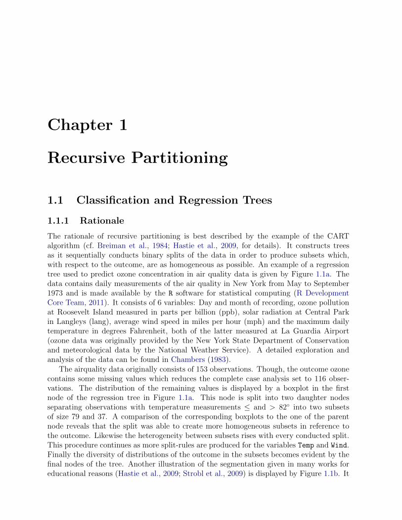
14 1. Recursive Partitioning
Compute the OOB accuracy of a tree.1.
Permute the predictor variable of interest in the OOB observations.2.
Recompute the OOB accuracy of the tree.3.
Compute the difference between the original and recomputed OOB accuracy.4.
Repeat step 1 to 4 for each tree.5.
The overall importance score is given by the average difference.6.
It can be read off equation (1.6) that the importance measure is based on the computationof the mean squared error (MSE) before and after permutation. Equation (1.5) inherentsthe accuracy which equals 1 - error rate = 1 - MSE for binary responses. This interpretationin terms of MSE is commonly used; as retraced in Nicodemus et al. (2010) for instance.Thus both measures are based on a statistic that is solely and directly derived from theresponse and the variable space. Good (2000) denotes the selection of an appropriatestatistic as step three in his listing of ’five steps to a permutation test’. The quality of sucha statistic is supposed to be its ability to discriminate between the null-hypothesis and thealternative. The MSE clearly satisfies this quality. Further examples of suitable statisticsfor permutation tests are given by Good (2005).
An example of permutation importance measures for the airquality data is given byFigure 1.8. As the original measure is not applicable to missing data these results emergefrom a complete case analysis. The next chapter introduces a new kind of importancemeasure which is able to deal with missing data and circumvents dangers associated withcomplete case analysis.
1.3 Statistical Software
All analyses and computations presented in this work were performed with the R systemfor statistical computing (R Development Core Team, 2011, version 2.14.1). It providesseveral freely available implementations of recursive partitioning: The CART algorithmis given by the function rpart() of the package rpart (Therneau et al., 2011, version3.1-52) and another implementation by tree() which is part of the tree package (Ripley,2011, version 1.0-29). In this work rpart() is used to represent the CART algorithm.Conditional inference trees and an implementation of conditional inference based RandomForests – called by ctree() and cforest() – are both included in the party package(Hothorn et al., 2008, version 1.0-0). Unfortunately the CART related implementationof Random Forests given by the function randomForest() in the package randomForest
(Liaw and Wiener, 2002, version 4.6-6) does not support the fitting of Random Forests

1.3 Statistical Software 15
Solar.R Wind Temp Month Day
Per
mut
atio
n Im
port
ance
0
200
400
600
800
Figure 1.8: Permutation accuracy importance for a complete case analysis of the airqualitydata.
to incomplete data. However, as the occurrence of missing values is in main focus of theinvestigations of this work and even more importantly: as it has been discussed in thischapter that the algorithm is prone to biased variable selection it is not used any further.Thus, Random Forests are executed by the function cforest(). A short summary offunctions used in this work is given in Table 1.2.
In this chapter the default settings for each function were used to perform the exemplaryanalyses. In the following chapters specific settings used for the analyses will be listedseparately.
Method Model Function Package Used
CART tree tree() tree
rpart() rpart XRandom Forest randomForest() randomForest
conditional tree ctree() party Xinference Random Forest cforest() X
Table 1.2: Summary of functions used to perform recursive partitioning.

16 1. Recursive Partitioning

Chapter 2
Predictive Accuracy for Data withMissing Values
2.1 Research Motivation and Contribution
The occurrence of missing values is a major problem in statistical data analysis. All scien-tific fields and data of all kinds and size are touched by this problem. A popular approachto handle missing values is the application of imputation methods (see Schafer and Gra-ham, 2002; Horton and Kleinman, 2007, for a summary of approaches). There is a numberof ad-hoc solutions – e.g. available case and complete case analysis as well as single imputa-tion by mean, hot-deck, conditional mean and predictive distribution substitution – whichcan lead to a loss of power, biased inference, underestimation of variability and distortedrelationships between variables (cf. Groenwold et al., 2012, for corresponding discussionsabout the proper analysis of missing outcome data in randomized trials and observationalstudies). A more promising approach of rising popularity is multiple imputation by chainedequations (MICE) also known as imputation by full conditional specification (FCS) (vanBuuren et al., 2006; White et al., 2011). It allows for the imputation of multivariate datawithout the need to specify a joint distribution of predictor variables. Furthermore, itssuperiority to ad hoc and single imputation methods has been shown by many publica-tions (e.g. Janssen et al., 2009, 2010). Alternatives to imputation are given by methodswith built-in procedures to handle missing values. This includes recursive partitioning byclassification and regression trees as well as Random Forests.
However there is only a few publications that compare the two approaches. Two ref-erence publications that investigate performance differences are given by Feelders (1999)and Farhangfar et al. (2008). Unfortunately, they lack generalizability as investigations arerestricted to classification tasks, categorical data and special simulation schemes. A thirdrelated paper that focuses on Random Forests is given by Rieger et al. (2010). It is basedon much more extensive simulation studies that involve different missing data generatingprocesses (section 2.3.1) for classification and regression problems.

18 2. Predictive Accuracy for Data with Missing Values
The goal of this chapter is to compare the predictive accuracy of CART, conditionalinference trees and Random Forests when surrogates and multiple imputation are used tohandle missing values. Comparative analyses for various datasets and different simula-tion settings are designed to improve and extend the investigations of related publications.Both classification and regression problems are examined. Findings show that multipleimputation produces ambiguous performance results for both simulation studies and em-pirical evaluations. By contrast, the use of surrogates is a fast and simple way to achieveperformances which are often only negligibly worse and in some cases even superior. Theinvestigations and findings of this chapter have been published in Hapfelmeier et al. (2011).
2.2 Discussion of Related Publications
• Feelders (1999) favors the application of imputation methods. This conclusion isbased on the investigation of two classification problems. The rpart() routine im-plemented in S (Becker, 1984), which closely resembles the CART algorithm proposedby Breiman et al. (1984) was applied. Procedures were compared by an assessment ofthe misclassification error rate (MER) which equals the fraction of wrong predictionsin the case of a binary outcome.
One of the examined datasets is the Pima Indians Diabetes Data Set (section 2.4.2).The MER of a tree that used surrogate splits was 30.6%. Single imputations basedon EM-estimates were repeated by ten independent draws and achieved an averagedMER of 26.8%; Little and Rubin (2002) clearly show that the variability of estimatesis likely to be underestimated by single imputation. Thus comparisons and testswithin each of the repetitions might be invalid. In a second experiment a multi-ple imputation approach was applied ten times. The averaged MER equals 25.2%.To back up the observed differences an exact binomial test was computed for eachrepetition. In the first experiment there were 6 of 10 and in the second experimentthere were 9 of 10 p-values below 0.05. Nevertheless a test for the comparison of twoproportions like the McNemar-Test would have been more appropriate. In additiononly the training data contained incomplete observations.
The second data is the waveform recognition data originally used by Breiman et al.(1984). Missing values were introduced completely at random in the training datain fractions between 10% and 45%. The imputation was performed by an LDAmodel based on EM-estimates. The MER of trees was assessed in two experimentswhich differed by the application of single imputation and multiple imputation. Forthe former the MER of a tree fit to imputed data was between 29.2% and 30.6%,seemingly unrelated to the fraction of missing values. Trees that used surrogate splitsproduced MER values between 29.8% and 34.3%. Results were similar for multipleimputation. The MER of trees with imputation lay between 25.5% and 26.1%. Withsurrogates the MER increased from 28.9% to 35.6%. Differences became more andmore pronounced with high fractions of missing values. However, 45% missing values

2.2 Discussion of Related Publications 19
in each variable is rather rare in real life data. A data set of only 5 variables wouldalready include 1 − (1 − 0.45)5 = 95.0% incomplete observations if the locations ofmissing values are statistically independent. Likewise an equal spread of missing datais rather artificial.
• Farhangfar et al. (2008) published a profound comparison of various classificationmethods applied to data with missing values. Several single imputation methods anda multiple imputation approach by polytomous regression using the MICE algorithmwere explored. Classification models were support vector machines (SVM), k-nearestneighbors (kNN), C4.5 (a decision tree algorithm introduced by Quinlan, 1993),among others. Missing values were induced into 15 completely observed datasetswhich exclusively consisted of qualitative variables. Results showed that the appli-cation of MICE, compared to other imputation methods, leads to superior results inmost cases. For none of the data sets the C4.5 method benefited from imputation.By contrast, the latter even led to worse MER values in some cases. The performanceof C4.5 was also independent of the amount of missing values. Like Feelders (1999)the authors restricted the occurrence of missing values to the training data. Theproblem of too many missing values equally spread among the variables was present,too. Up to 50% of observations per variable were set missing.
• In an extensive simulation study Rieger et al. (2010) concluded that the applicationof a k-nearest neighbors (kNN) imputation approach did not improve the perfor-mance of conditional Random Forests. Classification and regression problems withthree different correlation structures and seven schemes to generate missing valueswere investigated. These studies were repeated for high-dimensional settings withadditional noise variables and for two scenarios that differed by the introductionof missing values in the training and test data or solely in the training data. Thefraction of missing values was not varied and chosen to be two times 20% and onetime 10% in three variables. The comparison of approaches was based on predictionaccuracy measured by binomial log-Likelihood and mean squared error (MSE). Re-sults showed no clear advantage of imputation. Despite elaborate simulation settingsthe authors point out that results may not be generalizable due to specific choicesof parameters. However, this publication does not incorporate trees, uses a singleimputation method and does not vary fractions of missing values.
Feelders (1999) showed increased MER for an increasing number of missing values whensingle trees are used with surrogate splits. Meanwhile the MER of trees based on impu-tation almost did not change. Differences between methods were rather weak for lowerfractions of missing values which are more likely to be observed in real life data. Farhang-far et al. (2008) found no improvement for C4.5 Trees with imputed data. They evenclaim a harmful effect of imputation in this case. Pitfalls and drawbacks of the former twopublications are unrealistic simulation schemes, invalid test procedures, the application ofbiased imputation and tree building methods and the limited generalizability due to thepredominant examination of nonstandard polytomous data and classification tasks only.

20 2. Predictive Accuracy for Data with Missing Values
By contrast the work of Rieger et al. (2010) resolves many of these issues as it presents anextensive simulation study for classification and regression problems. The authors concludethat a k-nearest neighbor imputation approach was not able to improve the performanceof Random Forests.
2.3 Missing Data
2.3.1 Missing Data Generating Processes
In an early work Rubin (1976) specifies the issue of correct statistical inference from datacontaining missing values. A key instrument is the declaration of the process that causesthe missingness. Based on these considerations many strategies for inference and elaboratedefinitions of the subject have been developed. An extensive summary can be found inSchafer and Graham (2002). In general, three types of missingness are distinguished:
• Missing completely at random (MCAR):P (R|Xcomp) = P (R)
• Missing at random (MAR):P (R|Xcomp) = P (R|Xobs)
• Missing not at random (MNAR):P (R|Xcomp) = P (R|Xobs,Xmis)
The status of missingness (yes = 1/no = 0) is indicated by a binary random variable R andits probability distribution P (R). The letter R, that was adopted from the original nota-tion, may emerge from the fact that Rubin (1987) originally was dealing with ’R’esponserates in surveys. The complete variable space Xcomp is made up of observed Xobs andmissing Xmis parts; Xcomp = {Xobs,Xmis}. Therefore MCAR indicates that the probabilityof observing a missing value is independent of the observed and unobserved data. By con-trast for MAR this probability is dependent on the observed values (but not on the missingvalues themselves). Finally in MNAR the probability depends on unobserved informationor the missing values themselves. An example for the latter is a study in which subjectswith extreme values for an outcome systematically drop out while there is no informationin the data that could help to explain this discontinuation.
Farhangfar et al. (2008) outline that in practice the MCAR scheme is assumed for mostimputation methods. He et al. (2009) and White et al. (2011) point out that the MICEalgorithm is also capable of dealing with MAR schemes as the imputation model becomesmore general and includes more variables. In this situation it becomes more probablethat missing values can be explained by observed data. The latter property is especiallyvaluable for data that already contain missing data. In such settings it is not clear whichscheme really holds. Similar statements can be found in Janssen et al. (2010) which claimsthat even a false assumption of MAR under MNAR has minor impact on results in many

2.3 Missing Data 21
realistic cases. The performance of Random Forests under several MAR schemes wasinvestigated by Rieger et al. (2010). These authors compared the use of surrogates againsta single imputation method. In extensive simulation studies they were able to show thatresults did not differ between MCAR and MAR. For all these reasons the introduction ofmissing data is done in a MCAR scheme in the following simulation studies.
2.3.2 Multivariate Imputation by Chained Equations
Using MICE, imputation is performed by flexible specifications of predictive models foreach variable. There is no need to determine any joint distributions of the data. Cyclingthrough incomplete variables iteratively updates imputations until convergence. Repeatingthe procedure several times leads to multiple imputed data sets. A short summary of theoryand appealing properties is given in the following.
Multiple Imputation
A simple and popular approach to handle missing data is the application of multipleimputation (MI) as introduced by Rubin (1987, 1996). Little and Rubin (2002) point outthat an apparent advantage of this approach is its ability to make standard complete-datamethods applicable to incomplete data. Therefore the user is able to stick to his preferredmethod of analysis. There is no necessity to switch to one he is not used to, he does notunderstand or is known to be less powerful.
In general any measure of interest Q (e.g. parameter estimates θ or response predictionsy) is assessed by the average
QE =1
E
E∑e=1
Qe
using E estimates Qe derived from the imputed complete data sets. The total variabilityof the estimate is given by
TE = WE +E + 1
EBE
where
WE =1
E
E∑e=1
We and BE =1
E− 1
E∑e=1
(Qe −QE)2
are the average of the within-imputation variances We and the between-imputation vari-ance, respectively. Of course the essential preceding step is the creation of E imputed datasets. If imputation was only done once, like in single imputation, the imputed values wouldbe treated like they were known. This can lead to a severe underestimation of the vari-ance, ’which affects confidence intervals and statistical tests’ as stated by Harel and Zhou(2007). However, it is not sufficient to simply create more than 1 dataset by drawing from

22 2. Predictive Accuracy for Data with Missing Values
the conditional distribution P(Xmis|Xobs, θ). The uncertainty inherent in the estimate θitself has to be incorporated, too. The posterior predictive distribution of Xmis is
P(Xmis|Xobs) =
∫P(Xmis|Xobs, θ)P(θ|Xobs)dθ
with
P(θ|Xobs) ∝ P(θ)
∫P(Xobs,Xmis|θ)dXmis
denoting the observed-data posterior distribution of θ. A proper multiple imputationapproach is supposed to first draw E estimates θ(1), ..., θ(E) from P(θ|Xobs). These are
subsequently used in the conditional distributions P(Xmis|Xobs; θ(e)), e = 1, ...,E.
An example of this procedure was taken from Rubin (1987) and White et al. (2011) to
illustrate the case of parameter estimates θ = β for a linear regression model. Drawing fromits conditional distribution does not consider the uncertainty about the maximum likeli-hood estimate β. Thus β needs to be drawn from its posterior distribution P(β|Xobs), too.Under the assumption of ignorable nonresponse the estimation is based on the observeddata only. In a first step a linear regression is fit to the observed data which gives
βobs =(x>obsxobs
)−1︸ ︷︷ ︸V
x>obsyobs
and
σ2obs =
([(yobs − xobsβobs)
2]>
1
)/(nobs − npar).
npar is the dimension of β and nobs the number of observed values. When the prior distribu-tion on log σ is proportional to a constant it can be shown that σ2/σ2 follows an invertedχ2 distribution on n− 1 degrees of freedom. Based on these considerations the imputationstarts with the computation of
σ2∗ = σ2
obs(nobs − npar)/g
where g is a random number drawn from χ2nobs−npar
. Using the estimates σ2∗ and βobs, one
is able to compute
β∗ = βobs +σ∗σobs
[V]1/2z
where z is a vector that contains npar independent draws from a standard normal distribu-tion. [V]1/2 is the Cholesky decomposition of V. Finally,
ymis = xobsβ∗ + z∗σ∗.
Again z∗ is a vector of nmis independent random draws from a standard normal distribution.This procedure is repeated to generate several imputed data sets.

2.3 Missing Data 23
MICE
Whenever there is more than one variable with missing values the imputation approachneeds to be adapted. There are mainly two approaches for missing data imputation in thiscase. Joint modeling (JM) approaches, as presented by Schafer (1997), are not discussedin detail here. Still it is worth mentioning that imputations are directly drawn from theparametric multivariate density P(Xmis,Xobs,R|θ) by this approach. Appropriate methodsexist for the multivariate normal, log-linear and general location model. A more practicalapproach which makes it possible to bypass the specification of a joint distribution is MICEalso known as imputation by fully conditional specification (FCS) (cf. van Buuren, 2007;White et al., 2011). Although it lacks profound theory van Buuren et al. (2006) showed insimulation studies that MICE produces reasonable imputations and coverages of statisticsof concern. FCS, using linear regression, even equals JM under the multivariate normaljoint distribution, given specific regularity conditions. The same holds for some specialcases of the log linear model. According to van Buuren and Groothuis-Oudshoorn (2010)FCS is an attempt to obtain a posterior distribution of θ by chained equations. Theseauthors state that starting with the imputation of missing values by random samples ofthe observed values the tth iteration of the chained equations is
θt1 ∼ P(θ1|X1,obs,X
t−12 , ...,Xt−1
v ),
Xt1,mis ∼ P(X1|X1,obs,X
t−12 , ...,Xt−1
v , θt1),
...
θtv ∼ P(θv|Xv,obs,X
t1, ...,X
tv−1),
Xtv,mis ∼ P(Xv|Xv,obs,X
t1, ...,X
tv−1, θ
tv),
where Xtj is the jth imputed variable at iteration t. It is easy to see how turns are taken
within the iterative steps to infer θ and Xmis. After the convergence of the algorithmit is possible to draw θ from its posterior and to use it to obtain Xmis. Several imputeddatasets are produced by repeating the procedure with different starting values. A practicaladvantage of MICE are the many possibilities to model P(Xj|Xj,obs,X−j, θj). A profounddiscussion can be found in van Buuren and Groothuis-Oudshoorn (2010) and White et al.(2011). MICE is especially suitable in MAR settings although Janssen et al. (2010) statethat it should also be preferred to ad hoc methods like complete case analysis even inMNAR situations. In a review paper of epidemiologic literature Klebanoff and Cole (2008)conclude that MICE is still of minor popularity. Despite its outstanding benefits comparedto simpler ad hoc methods it seems like researchers feel uncomfortable to use it. Thus theygive recommendations about the proper publication of multiple imputation methods toincrease their popularity. These are followed in this chapter and outlined in section 2.4.3.
To date there are still proposals for further developments. For example Burgette andReiter (2010) claim that complex distributions as well as interactions and nonlinear rela-tions might better be fit using CART as imputation model within the MICE algorithm.They are able to present promising results in a simulation study and an application toreal life data. Likewise, Stekhoven and Buhlmann (2011) present an iterative approach

24 2. Predictive Accuracy for Data with Missing Values
that uses Random Forests to impute missing values and show its superior performance inempirical evaluations; especially when there are complex interactions and nonlinear rela-tions. Templ et al. (2011) emphasize that many imputation approaches ‘...assume that thedata originate from a multivariate normal distribution...’. They suggest an iterative robustmodel-based imputation procedure to deal with data that deviate from this assumption(e.g. data that contain outliers or originate from skewed or multimodal distributions).Accordingly, future studies should take the diversity of MICE approaches into account.
2.4 Studies
In order to explore several kinds of data which display a random sample of real life situationswith a wide range of attributes there were no constrictive exclusion criteria applied for theirselection. There are 12 datasets; half of them were supposed to contain regression and halfof them classification problems. Four datasets without any missing values were used fora simulation study and the remaining eight datasets, that contained missing values inadvance, were used for an application study. There were no restrictions about the numberof observations or variables and the amount of missing values. The datasets were includedwithout any prior knowledge of these characteristics or any presumptions about potentialfindings. Therefore a broad set of data emerging from different scientific fields was used.
There are two kinds of studies. The first one is meant to retrace and extend the simu-lations discussed in section 2.2. The introduction of missing values was varied for a deeperinsight to effects caused by special schemes. The second study is based on empirical evalu-ations of data that already contain missing values. It is supposed to provide a more reliableassessment of potential benefits of imputation without the need of artificial specificationsfor the simulation settings. To stick close to existing publications, the performance assess-ment is given by the mean squared error (MSE). This measure equals the misclassificationerror rate (MER) for binary responses.
Evaluation is done by Monte-Carlo Cross-Validation (MCCV; see Boulesteix et al.,2008b). Analyses are performed for two cases that differ by the decision to use imputationthrough MICE or surrogates. It is well known that for valid evaluations the test dataneed to be isolated from the training data in every aspect. This can only be achieved iftwo separate imputation models are fit to each of these datasets. Otherwise it is believedthat the MSE estimation would be positively biased as an imputation model fit to thetraining data and applied to the test data would transfer information. One could not callthe observations of the test data ‘unseen’ to the predictive model any more. Consequently,separate imputation models were fit to the training and test dataset. Of course the responseis also not allowed to be part of the imputation model for the test data. It is consideredunknown until the comparison of predicted and real outcomes for evaluation purposes.

2.4 Studies 25
2.4.1 Simulation Studies
Analysis settings
Data were MCAR in the simulation studies. Thus each value had the same probability tobe missing independent of any observed or unobserved information. Four datasets werechosen for the simulation studies as they were fully observed. Two of them are used forthe classification of a binary response. Another two are used for regression. Missing valueswere artificially introduced in a procedure which is close to the one of Feelders (1999) andFarhangfar et al. (2008). However, the introduction of missing data was not restrictedto the training set but extended to the test set, too. Fractions of missing values are 0%(benchmark), 10%, 20%, 30% and 40%. The procedure was repeated 1000 times usingMonte-Carlo Cross-Validation (MCCV). In each iteration a random sample of 80% wasused for the training of a model while the remaining 20% served as test set. This alsofacilitated the separation of imputation models for the training and test data.
Part of the criticism in section 2.2 was about the huge amount of missing values whichis beyond the fractions found in most of real life data; the number of observations thatcontain at least one missing value is 1 − (1 − %missing)nvariables which, on average, alreadymakes 1− (1− 0.40)5 = 92.2% incomplete observations for a dataset that contains only 5variables with 40% missing values. To stick closer to real life situations the simulation wasrepeated with a randomly chosen third of the variables partly set missing in each MCCVstep. The corresponding R-Code is given in the appendix B.2.1.
Data
A summary of the data is given by Table 2.1 and the following listing:
• Haberman’s Survival Data contains data about the 5 year survival of patientsafter breast cancer surgery. It was originally used for investigations of log-linear mod-els by Haberman (1976). The corresponding study was conducted between 1958 and1970 at the University of Chicago’s Billings Hospital. There are 306 observations in 3independent variables namely age, year of operation and number of positive axillarynodes. The survival status of a patient was used as the outcome of a classificationproblem.
• The Heart Disease Data was collected at four clinical institutions. These arethe Cleveland Clinic Foundation, the Hungarian Institute of Cardiology, Budapest,the V.A. Medical Center, Long Beach, CA and the University Hospital, Zurich,Switzerland. It contains information about the incidence of heart disease along withthe assessment of a patients age, gender, chest pain type, resting blood pressure,serum cholestoral in mg/dl, a fasting blood sugar measurement (> 120 mg/dl), restingelectrocardiographic results, maximum heart rate achieved, exercise induced angina,ST depression induced by exercise relative to rest, the slope of the peak exerciseST segment, number of major vessels (0–3) colored by flourosopy and thallium scanstatus information. These socioeconomic data and clinical outcomes were used to

26 2. Predictive Accuracy for Data with Missing Values
classify the binary outcome, i.e. heart disease. The data contain 270 observationsand 13 independent variables.
• The Swiss Fertility and Socioeconomic Indicators Data contains a standard-ized fertility measure and socio-economic indicators. It was originally used for re-gression analysis by Mosteller and Tukey (1977). Features are percentages of malesinvolved in agriculture, draftees receiving highest mark on army examination, drafteeswith education beyond primary school, catholic population and the infant mortalitywithin the first year of life. Data were gathered in 47 French-speaking provinces ofSwitzerland at about 1888; this makes 47 observations in 5 independent variables.The regression aims at the explanation of the standardized fertility measure in eachprovince.
• The Infant Birth Weight Data was collected at the Baystate Medical Center,Springfield, Mass during the year 1986. It contains physical measures and informa-tion about the health condition of women giving birth. Venables and Ripley (2003)originally used it for a classification of the binary outcome, low and high birth weightof newborns. Here, by contrast, a regression was performed to predict a child’s birthweight in grams by the means of a mother’s health status and history. The lat-ter is given by a mother’s age in years, weight in pounds at last menstrual period,race, smoking status during pregnancy, number of previous premature labors, historyof hypertension, presence of uterine irritability and the number of physician visitsduring the first trimester. The data contain 189 observations and 9 independentvariables.
It has to be pointed out that for the Heart Disease Data and the Infant Birth Weight Datathe number of predictor variables was reduced to 12 and 8, respectively. This was dueto computational issues with the MICE implementation, which might be seen as anotherdisadvantage of this approach, but only touches the analyses of this chapter.
Data Obs. ind. Var.
H. Survival 306 3Heart 270 13Fertility 47 5Birthweight 189 9
Table 2.1: Count of observations and independent variables for datasets used in the simu-lation studies.

2.4 Studies 27
2.4.2 Empirical Evaluation
Analysis settings
Although simulation studies might be helpful to investigate theoretical properties thereare some deficiencies in the simulation schemes that clearly limit generalizability of results.Corresponding statements have been discussed in section 2.2. Thus, the main focus ofthis chapter is put on empirical evaluations of data that originally contain missing values.A total of eight datasets has been used to explore four classification and four regressionproblems. Again, each data was split in 1000 MCCV runs into 80% training and 20%test observations to estimate a method’s performance in terms of MSE. The correspondingR-Code is given in the appendix B.2.2.
Data
The eight datasets summarized in Table 2.2 are:
• The Hepatitis Dataset contains information about 155 patients that suffered fromhepatitis and of whom 32 died. A total of 19 independent variables is available forthe classification problem to predict a patient’s survival. These variables includedemographic data like sex and age, information about drug intake like steroids andantivirals and further clinical factors. One missing value was observed in 4 variables,5 missing values in 4 variables, and 4, 6, 10, 11, 16 and 29 missing values in onevariable, respectively. Therefore missing values were present in 14 out of 18 variables.The fraction of missing values per variable ranges from 0.6% to 18.7%. In total 43(27.7%) observations contain at least one missing value.
• The Mammographic Mass Data is made up of several features extracted frombreast cancer screenings. The latter are performed by physicians, especially radiol-ogists, who try to determine the severity (benign or malign) of a suspicious lesion.In the recent past efforts have been made to solve the classification problem by ma-chine learning approaches. The resulting systems are called CAD (Computer AidedDecision/Detection) systems. The data were originally used by Elter et al. (2007) forthe evaluation of such systems (c.f. Hapfelmeier and Horsch, 2011, for correspondingevaluation studies). Analyses were performed to describe the severity status of alesion. The data also contain information about the four independent variables age,shape, margin and density of mass lesions observed in 961 women. Age contains5 missing values while shape, margin and density are missing 31, 48 and 76 times,respectively. The corresponding fractions of missing values are 0.5%, 3.2%, 5.0% and7.9%. Overall 130 (13.5%) observations contain at least one missing value.
• The Pima Indians Diabetes Dataset was also used for the comparison of treeswith and without imputation by Feelders (1999). It contains information about thediabetes disease of 768 pima indian women which are at least 21 years old. In additionto age, the number of pregnancies, plasma glucose concentration, diastolic blood

28 2. Predictive Accuracy for Data with Missing Values
pressure, triceps skin fold thickness, 2-Hour serum insulin, BMI and diabetes pedigreefunction were recorded. This makes 8 independent variables used for the classificationproblem to determine whether a women shows signs of diabetes according to theWHO definition.
At first glance these data do not seem to contain any missing values. However, themissing values are actually “hidden” behind many zero values that are biologicallyimplausible or impossible. Pearson (2006) calls this situation “disguised missingdata” and gives a profound discussion about its occurrence in the Pima IndiansDiabetes Data Set. According to his description, there are five variables that containmissing data. The total numbers of missing values in these variables are 5, 35, 227,374 and 11, which equals fractions of 0.7%, 4.6%, 29.6%, 48.7% and 1.4%. Overall376 (49.0%) observations contain at least one missing value.
• The Ozone Level Detection Dataset was collected from 1998 to 2004 at theHouston, Galveston and Brazoria area and contains information about geographicmeasures and ozone levels. The classification problem is to distinguish days of highand low ozone concentration based on information about wind speed, temperature,solar radiation etc. In total there are 2534 observations in 73 measured features.Each of the variables contains between 2 (0.08%) and 300 (11.8%) missing values.For the entire data 687 (27.1%) observations contained at least one missing value.
• The Airquality Dataset contains daily measurements of the air quality in New Yorkfrom May to September 1973. There are four variables that were of interest for theplanned analyses. These are the ozone pollution in parts per billion (ppb), the solarradiation in Langleys (lang), the average wind speed in miles per hour (mph) andthe maximum daily temperature in degrees Fahrenheit (degrees F). The ozone datawere originally provided by the New York State Department of Conservation and themeteorological data by the National Weather Service. A more detailed explanationof the data can be found in Chambers (1983). All of the metric variables were usedto predict the temperature in a regression problem. For 153 days the ozone pollutioncontains 37 (24.2%) missing values while the solar radiation contains 7 (4.6%). Thereare 42 (27.5%) observations that have at least one missing value.
• The El Nino Dataset was gained from the Tropical Atmosphere Ocean (TAO) ar-ray of the international Tropical Ocean Global Atmosphere (TOGA) program. TAOis an assemblage of ca. 70 moored buoys that record oceanographic and surface me-teorological variables in the equatorial pacific. The present data contain informationabout four independent variables, i.e. the sea surface temperature, air temperature,humidity as well as zonal and meridional wind speeds. The regression problem wasto predict the sea surface temperature from the remaining variables. There are 733observations of which 78 (10.6%) and 91 (12.4%) are missing for the air tempera-ture and the humidity, respectively. For the entire data 168 (22.9%) observationscontained at least one missing value.

2.4 Studies 29
• The CHAIN Project Data contains information from a longitudinal cohort studyof HIV infected people living in New York City by 1994. It was originally used byMesseri et al. (2003) for the assessment of HIV treatment effects on survival. Forthe planned analyses there were 508 observations of seven variables. These are thelog of self reported viral load level, age at time of interview, family annual income, acontinuous scale of physical health, the CD4 count, a binary measure of poor mentalhealth and an indicator for the intake of HAART. The regression problem was toexplain the continuous scale of physical health. There were 155 missing values inthe self reported viral load level, 14 in the family annual income and 39 in the CD4count. This equals fractions of 30.5%, 2.8% and 7.7%. At least one missing value inany variable was observed for 173 (34.1%) observations.
• The Mammal Sleep Data contain features of 62 species ranging from mice overopposums and elephants to man. It was originally used by Allison and Cicchetti(1976) to examine relations between sleep, ecological influences and constitutionalcharacteristics. The observed sleep features include information about duration anddepth of sleep phases as well as the occurrence of dreams. Constitution is givenby measures like body weight and brain weight. The safety of sleep is assessed byscaling for overall danger, danger for being hunted, sleep exposure, gestation timeetc. One of the main findings in the original paper was a negative correlation betweenslow-wave sleep and body size. In alignment with these investigations the data wasused in a regression analysis for the prediction of body weight. The data contains 9independent variables and 62 observations. There are 20 (32.3%) observations whichare not completely observed for all variables. It is interesting to note that Allisonand Cicchetti (1976) had originaly chosen a complete case analysis as they found theincomplete data to be “... not suitable for the multivariate analyses ...”. There arefive variables containing 4 (3 times), 12 and 14 (6.5% (3 times), 19.4% and 22.6%)missing values.
Most of the data is provided by the open source UCI Machine Learning Repository (Frankand Asuncion, 2010). However, the Fertility and Airquality Data were taken directly fromthe R routine. Likewise, the Birthweight, CHAIN Project and Sleep Data are part of theR packages MASS, MI and VIM, respectively.
2.4.3 Implementation
All analyses were performed with the R software for statistical computing (R Develop-ment Core Team, 2011, version 2.14.1). The CART algorithm is provided by the functionrpart() which is part of the equally named package rpart (Therneau et al., 2011, version3.1-52). It is opposed to conditional inference trees called by ctree() which is part of theparty package (Hothorn et al., 2008, version 1.0-0). This package also includes the func-tion cforest() which is used for the implementation of Random Forests. Unfortunatelythe function randomForest() in the package randomForest (Liaw and Wiener, 2002, ver-sion 4.6-6) does not support the fitting of Random Forests to incomplete data. Thus,

30 2. Predictive Accuracy for Data with Missing Values
Observations VariablesData # ≥ 1 missing # missing per Var.
Hepatitis 155 43 (27.7%) 19 14 (0.6% – 18.7%)Mammo 961 130 (13.5%) 4 4 (0.5% – 7.9%)Pima 768 376 (49.0%) 8 5 (0.7% – 48.7%)Ozone 2534 687 (27.1%) 73 73 (0.1% – 11.8%)Airquality 153 42 (27.5%) 4 2 (4.6% – 24.2%)El Nino 733 168 (22.9%) 4 2 (10.6% – 12.4%)CHAIN 508 173 (34.1%) 7 3 (2.8% – 30.5%)Sleep 62 20 (32.3%) 9 5 (6.5% – 22.6%)
Table 2.2: Characteristics of datasets used for the empirical evaluation. The numberof independent variables and observations is given in addition to absolute and relativefrequencies of missing values among them.
this biased, CART based version could not be used for comparison matters. MultivariateImputation by Chained Equations was done by the mice() function of the mice package(van Buuren and Groothuis-Oudshoorn, 2010, version 2.11).
The number of trees in Random Forests was set to be ntree = 500. Each split waschosen from mtry = min(5, variables available) randomly selected variables. Trees andRandom Forests use maxsurrogate = min(3, variables available) surrogate splits. MICEproduces five imputed datasets. A normal linear model was used for the imputation ofcontinuous variables, logistic regression for binary variables and a polytomous regression forvariables with more than two categories: defaultMethod = c(”norm”, ”logreg”, ”polyreg”).Concerning the training data each variable contributed to the imputation models. In thetest data the response was excluded from these models. The fraction of imputed valuesand number of variables used for imputation can be read off Table 2.1 and 2.2.
2.5 Results
2.5.1 Simulation Studies
The following contains discussions for each of the four investigated datasets. A correspond-ing graphical representation is given by Figure 2.1. A summary of observed MSE values ispresented by Table 2.3 and an even more elaborate listing is given in the appendix A.1.1.
• Haberman’s Survival Data is used to predict the 5 year survival of patients afterbreast cancer surgery. Random Forests, ctree and rpart perform comparably. Theyare able to preserve the benchmark MSE (obtained for 0% missing values) indepen-dent of the procedure to handle missing values. The relative improvement by MICEinstead of surrogates ranges from -2% to 5% and gets even less pronounced (-2% to1%) when only one third of variables contains missing values.

2.5 Results 31
• By means of the Heart Disease Data it is assessed how well the presence of heartdisease can be predicted. In terms of prediction accuracy, Random Forests outper-forms both single tree methods, while rpart produces slightly superior results thanctree. An increased number of missing values makes error rates rise especially whenthey are introduced in each variable. The relative improvements by MICE shrinkfrom a range of 0% to 22% to a range of -5% to 2% when only one third of variablescontain missing values.
• The Swiss Fertility and Socioeconomic Indicators Data is used to examinewhether a continuous fertility measure can be explained by socio-economic indicators.All three methods produce comparable results. Although in some instances, one isable to produce results which are close to the benchmark when surrogates are usedit is obvious that MICE results exceed this level. A slight rise in differences betweenmethods can be observed for an increased number of missing values. The meanrelative improvement due to imputation is between 1% and 19%. When there aremissing values in only one third of the variables this relative improvement rangesfrom -2% to 4%.
• The Infant Birth Weight Data is used to predict a child’s birth weight in grams.Random Forests clearly outperform its competitors while ctree and rpart performcomparably. The difference between imputation and surrogates does not increasewith an increased number of missing values. In some cases MICE makes the perfor-mance exceed the benchmark. The improvements by imputation drop from 2%–7%to 0%–4% when the number of variables that contain missing values is restricted toone third.
Referring to single trees it has to be stressed that a comparison between the application ofMICE and surrogates is not quite fair. MICE produces multiple datasets that vary in theimputed values. To each of them a tree is fit which may consequently differ from each other.Their average or majority decision for an observation is used for prediction. Several works(e.g. Buhlmann and Yu, 2002; Breiman, 1996) show that ensemble approaches performsuperior to single trees. This fact becomes apparent for the Swiss Fertility Data as MICEis able to even exceed the benchmark obtained for 0% missing values. By contrast RandomForests are an ensemble method themselves which makes them less prone to this effect.Therefore, one might find them even more suitable for a fair comparison. Anyhow as MICEis very popular this multiple imputation approach is still preferred to single imputation inorder to reflect use-oriented results.
2.5.2 Empirical Evaluation
Results obtained for the eight investigated datasets which originally contain missing valuesare displayed by Figure 2.2. The relative improvement of MICE compared to the applica-tion of surrogates can be read off Table 2.4. An extensive listing of results can be foundin the appendix A.1.2.

32 2. Predictive Accuracy for Data with Missing Values
missing valuesmissing 0% 10%–40% 10%–40%
Type Data Model variables benchmark Surrogates MICE rel. imp.Classi- H. Survival forest 3 0.27 0.28 – 0.29 0.27 0% – 5%fication 1 0.27 0.27 0%
ctree 3 0.28 0.27 – 0.28 0.27 – 0.28 -2% – -1%1 0.27 – 0.28 0.28 -2% – -1%
rpart 3 0.28 0.28 0.28 -2% – 0%1 0.28 0.28 -1% – 0%
Heart* forest 12 0.17 0.19 – 0.26 0.18 – 0.23 0% – 7%4 0.18 – 0.19 0.18 – 0.19 -5% – -2%
ctree 12 0.24 0.27 – 0.35 0.24 – 0.27 7% – 22%4 0.25 0.25 -2% – 0%
rpart 12 0.22 0.23 – 0.30 0.21 – 0.25 6% – 13%4 0.22 – 0.23 0.21 – 0.22 -1% – 2%
Regres- Fertility forest 5 124 129 – 160 123 – 129 1% – 17%sion 2 123 – 131 122 – 129 -2% – 0%
ctree 5 126 144 – 164 116 – 126 12% – 19%2 126 – 136 119 – 125 1% – 4%
rpart 5 128 129 – 143 113 – 121 5% – 9%2 121 – 132 115 – 125 -1% – 2%
Birthweight* forest 8 46e+4 48e+4 – 52e+4 47e+4 – 51e+4 2% – 3%3 46e+4 – 48e+4 46e+4 – 48e+4 0% – 1%
ctree 8 52e+4 54e+4 – 56e+4 51e+4 – 53e+4 4% – 7%3 52e+4 – 54e+4 51e+4 – 52e+4 2%
rpart 8 53e+4 54e+4 – 56e+4 51e+4 – 54e+4 3% – 5%3 53e+4 – 55e+4 51e+4 – 52e+4 3% – 4%
Table 2.3: Summary of mean MSE values and mean relative improvements (rel. imp. =MSESur.−MSEMICE
MSESur.) obtained by multiple imputation and surrogates. Please note that the
mean relative improvement is given by the mean of improvements across simulation runs.It can not simply be computed by the mean MSE values used in the formula given here(as the mean of ratios does not equal the ratio of means). *The predictor sets of 13 and 9variables were reduced to 12 and 8 variables due to computational issues with the MICEimplementation.

2.5 Results 33
●●● ●
●●●●●
●● ●●●●● ●●●
●●
●
●
●●●●
●
●●
●
●
●
●
●●
●●●
●
●
●
●●●
●
●●
●●●●
●●
●●● ●
●●
●
●
●●●●●
●
●●
●
●●
●
●●●
●
●●●●●
●●●
●●
●
●●●●
●
●●●
●
●●●
●
●●●
●
●●●●●
●
●●●
●
●●
●
●
●
●●●●●●●●●
●●
●
●●● ●●●●●●●●●●
●
●●●
●
●●●●●●
● ●●●●●
●
●●
●
●
●
●●●●
● ●●●●
●●●●●●●●●
●●
●●
●
●
●●
●
●●●
●
●
●
●
●
●●
●
●
●
●
●
● ●
●●●●●●
●●●● ●
●● ●
●●●●●●●●●●●● ●●●●●●●●●●● ●
●
●
●
●●
●●
●●
●
●●
●
●●●●
●
●
●
●●
●
●●●●● ●●●●●
●●
●●●●
●
●●●●●●●●● ●
●
●●●●●●● ●●
●
●
●●●●●
●
●● ●●
●
●
●●●●●
●
●● ●
●●●●
●●
●
●
●
●
●●
●●●
●
●●
●
●●●
●
●●●
●
● ●●●●
●
●●●●
●
● ●●●
●●
●●●●●
●
●
●
●
●●
●●
●
●● ●●●●●●●
●
●
●
●
●
●
●
●●
●●●
●
●●
MS
E
0.0
0.1
0.2
0.3
0.4
0.5
0.6
0.0
0.1
0.2
0.3
0.4
0.5
0.6
10% 20% 30% 40% 10% 20% 30% 40% 10% 20% 30% 40% 10% 20% 30% 40% 10% 20% 30% 40% 10% 20% 30% 40%
SUR.IMP.random forest ctree rpart random forest ctree rpart
1/1 of variables (#3) contain missings 1/3 of variables (#1) contain missings
● ●●
●●
● ● ● ● ● ● ● ● ● ● ●● ● ● ● ● ● ● ● ● ● ● ● ● ● ● ●
● ● ● ● ● ● ● ● ● ● ● ● ● ● ● ●
●●●●
●
●●
●●
●●●●
●
●
●●●
●●
●
●
●●●●
●
●●
●●
●●
●
●●
●●
●
●● ●
●
●
●●●●
●
●●●●
●●
●●●●
●
●●
●
●
●
●●
●
●
●
●
●
●
●
●
●
●
●
●
●
●
●●●
●●●●●
●
●●
●
●
●●
●●
●
●●
●
●
●●
●
●●●
●
●
●
●
●
●●●
●
●●
●
●
●●●
●
●
●●●●
●
●
●●
●
●●●●
●
●●
●●
●
●
●
●●
●
●
●
●
●
●●
●
●
●●●
●●
●●●
●
●
●
●
●
●
●●
●
●
●●
●
●●
●
●
●●●
●●●
●
●●
●●
●
●●●●
●
●
●
●
●
●●
●
●
●
●
●●
●●●●
●●●
●
●
●
●
●
●
●●
●
●●
●●
●
●●
●
●
●
●
●
●●●
●
●●●
●
●
●●
●●●●
●
●
●●●
●
●
●
●
●
●
●●
●
●●
●
●
●
●●
●
●
●
●
●
●
●
●
●
●●●●
●
●
●
●
●
●
●●
●
●
●
●
●
●
●●
●
●●
●
●●
●
●
●
●
●●
●●
●
●
●
●
●●●
●
●
●
●
●●
●
●
●
●
●
●●
●
●
●
●●
●
●
●
●
●
●
●●
●
●
●
●
●
●
●●●
●●
●
●
●
●
●●
●
●
●
●
●
●
●
●
●●
●●●●
●
●●
●●
●
●
●
●●
●●●
●
●●●
●
●●●●●
●
●
●●
●
●
●●
●
●●●●
●
●
●●●●●●
●
●
●
●
●
●●●
●
●
●
●
●
●
●
●
●
●
●●●
●●●●
●
●●
●
●●
●
●
●
●
●
●
●●
●●
●
●
●
●
●
●
●
●
●
●
●
●●
●
●●
●
●●●●
●●
●●
●
●
●
●
●
●
●
●
●●
●
●●
●●
●
●
●
●
●
●
●
●●
●
●
●
●●●●
●
●
●
●●
●
●
●●
●
●
●
●
●
●
●
●
●
●
●●●
●
●
●
●
●
●
●●
●●
●
●
●
●
●
●●
●●
●
●
●
●
●●●●
●
●
●
●
●●
●
●
●
●
●●
●
●
●●●
●
●●●
●
●
●
●
●
●
●●●
●
●
●●
●
●
●
●●
●
●
●
●
●
●
●
●
●●
●
●
●
●
●●
●
●
●●
●
●
●
●●
●
●
●
●
●
●
●●●
●
●●
●●●●●
●
●●
●
●
●
●●●●
●
●
●●
●●
●
●●
●
●
●
●
●
●●
●
●
●
●
●●
●
●
●
●
●●
●
●
●●●
●●
●
●
●
●
●
●
●
●
●●
●
●
●
●
●
●
●
●
●
●
●
●
●
●●●
●
●
●
●
●
●
●
●●●●
●
●●
●
●
●●
●
●
●●
●
●●●
●
●
●
●
●●
●●●
●
●
●●●
●
●
●
●
●●
●
●●
●●●
●
●
●
●
●●●
●
●●
●
●
●
●●
●
●
●●●
●
●
●
●
●
●
●
●
●
●
●
●●
●●●●
●
●
●
●
●●
●
●
●
●
●
●●
●
●
●
●
●●
●
●●
●●●●●
●
●●●
●
●
●●●●●
●
●
●
●
●
●●●
●
●●
●
●
●
●
●●
●
●
●●
●
●
●
●
●
●
●
●
●●●●
●
●
●
●
●
●
●
●
●
●
●
●
●
●
●
●
●
●
●●
●●
●
●
●
●
●
●
●
●●
●
●
●
●
●
●
●
●●
●
●
●
●
●
●
●
●
●
●
●●
●
●●
●●
●
●
●
●
●
●●●●
●
●
●
●●
●
●●●
●
●
●●
●●
●●●
●
●
●
●
●●
●
●●
●
●●●
●
●
●
●●
●
●●
●
●
●
●
●
●
●
●
●●
●●●●
●●
●
●
●
●
●
●●
●
●
●
●
●●
●
●
●
●
●
●
●
●
●
●
●
●
●
●
●●●
●
●
●
●
●
●
●●
●
●
●
●●●
●
●
●
●
●
●
●●
●
●●
●
●●
●●●
●
●
●
●
●●
●
●
●
●
●
●
●
●
●●●●●●
●
●
●●
●
●
●●
●
●
●●
●
●
●
●
●
●
●
●
●●
●
●●●●
●
●
●
●●●
●
●●
●
●
●●
●●●
●●
●
●
●
●
●
●
●●
●
●
●
●
●
●
●●●●
●
●
●
●
●●●
●
●
●
●
●
●●●
●
●
●
●
●●
●
●
●●
●●●●●
●●
●
●●●●●
●
●
●●
●
●
●
●
●●
●●●
●
●
●
●
●
●●
●
●
●●●●●
●
●
●
●●●●●
●●●
●●●●●●●
●
●●
●●
●
●●
●
●
●
●
●
●
●
●
●●
●
●
●
●
●●
●
●●●●
●
●
●
●
●
●
●
●
●
●
●
●
●
●
●
●
●●●
●
●●
●●
●
●
●●
●
●●
●●●●●●
●●
●●●
●●
●
●
●
●
●
●
●
●
●
●
●
●●
●
●
●
●
●
●
●
●
●●
●●●●●
●
●
●●●
●
●
●
●●●
●●
●
●
●
●
●●●●
●
●
●●●
●●●
●
●●
●●●
●
●
●
●●
●●
●
●●
●
●●●
●
●
●
●
●
●
●
●
●●●
●
●
●
●
●●●
●●●
●
●
●
●
●●●
●
●●●●
●
●●
●
●
●
●
●
●●
●
●
●
●
●●
●
●
●
●
●
●●
●●
●
●
●●●
●
●
●
●
●
●
●
●
●
●
●●
●
●●
●
●
●
●
●
●
●
●
●
●
●
●
●
●
●●●●
●
●
●●
●
●
●●
●
●
●
●●●
●
●
●
●●●●●
●
●
●●
●
●●
●
●●●
●
●
●●
●
●
●
●
●
●●
●●●
●
●●
●
●
●●●●
●
●
●●●
●
●●
●●●
●
●●
●
●
●
●
●
●●
●●
●●●●●●
●
●●
●
●●●●●●
●●●
●
●
●
●
●●
●
●
●
●
●●
●
●
●
●
●
●
●
●
●
●
●
●
●
●
●●●
●●●
●●
●
●
●
●
●
●●
●●
●
●
●
●
●●
●
●
●
●
●
●
●
●
●
●●●
●
●
●●
●●
●●
●●●●●
●●
●●
●
●●●
●
●
●
●
●
●
●
●
●●
●
●
●
●
●
●
●
●
●●●
●
●●●●
●
●●●
●
●●
●
●
● ●●●●●
●
●●
●
●●●
●●
●●●●●●●
●
●
●●●●●
●●
●●●●●
●
●
●
●
●
●
●
●●
●●
●●
●
●
●
●
●
●
●●●●●●●●●●●●●●
●
●
●●
●
●●●
●●
●●●●
●●
●●●● ●
●●
●
●●●
●●●●
●●●
●
●
●●●●●
●
●●
●
●
●
●●●●
●
●●
●
●
●
●
●
●
●
●
●
●
●
●
●●●●●
●●●●●
●●
●
●●
●
●
●
●●
●
●
●
●●
●
●
●
●
●
●
●
●
●
●
●
●
●
●●●●
●
●
●
●
●●●
●
●●
●
●●●
●
●●●●●●
●
●●
●
●
●
●●
●
●
●
●●●
●
●
●
●●
●●
●●
●
●●
●●
●
●
●●
●
●
●●
●
●
●
●
●●
●
●
●
●●
●
●
●
●
●
●●●
●
●●
●
●
●
●●
●
●
●
●
●
●
●
●●●
●
●
●●●●
●
●
●
●
●
●
●
●
●
●
●●●●
●●●●●
●
●●
●
●●
●
●
●
●
●
●
●●
●●
●
●
●
●●
●●
●
●
●●
●
●
●
●
●
●●
●
●
●
●
●
●●●●●
●●●
●
●●●●
●
●●
●
●
●●
●
●
●
●
●
●
●
●
●
●●
●
●
●●
●●
●●
●
●●
●
●
●
●●●
●●
●●
●●●●●●●
●
●
●
●●
●●●
●
●
●
●
●
●
●●
●
●
●
●
●●●●
●●
●
●
●
●
●●●
●
●●
●●●●●
●●
●
●
●
●
●
●●
●
●●●
●
●
●
●●
●
●●●
●
●
●
●●
●
●
●
●
●
●
●
●●
●
●●
●
●●
●
●
●
●
●
●●●
●
●●
●●●
●●
●
●
●●●●●
●
●
●
●
●●
●
●
●●
●
●
●
●
●
●
●
●
●
●
●●
●
●
●●
●
●●
●
●
●●
●
●
●
●
●
●●
●
●●●
●●
●
●
●●●●
●●●●●
●●
●
●
●
●
●
●
●
●●●
●●
●
●
●●
●
●
●
●
●
●
●
●
●
●
●
●
●●
●
●
●●●●●●●
●
●
●
●
●●
●●●●●●
●●●
●
●
●
●●●●
●
●●
●
●●
●
●
●
●●
●●
●
●
●
●
●
●●●
●
●
●●●●
●
●
●
●
●
●
●
●
●
●
●
●
●
●
●
●
●
●
●
●
●●●
●●
●
●
●
●
●
●●●
●●
●
●
●●
●
●
●
●
●
●●
●●
●
●●●
●●
●
●
●●●●●
●
●
●
●●●
●
●●
●
●
●
●●●
●
●●
●
●
●
●
●
●
●●
●●●●
●
●
●
●
●●●●●
●●●
●
●
●
●●
●●
●
●●●
●
●
●
●●
●●
●
●●
●
●
●
●●
●
●
●●●●
●
●
●
●●●
●●●
●●
●
●
●
●●
●
●●
●
●
●
●
●
●
●●●
●
●
●
●●
●●●●
●●
●●
●●●
●●●
●
●
●
●
●●●
●
●●●
●
●●
●
●●●
●
●●
●●●
●
●
●
●
●
●
●
●●
●
●
●
●
●●
●
●●●●
●●●
●●
●
●
●
●
●
●
●
●●●
●●●
●
●
●●
●
●
●
●
●●
●
●●●
●
●●
●●
●
●
●
●
●
●●●
●
●
●
●
●●
●
●
●
●
●
●●
●
●●
●
●●
●●
●●●
●●
●
●●●●●●●
●
●
●●
●
●●
●
●●
●
●●●
●●
●
●●
●●●●●
●●
●
●
●
●
●●●
●
●●●
●
●
●
●●
●
●
●
●
●●
●
●
●●
●
●●
●
●
●
●
●●●
●
●
●
●
●
●●
●
●
●●
●●
●●●●
●
●
●●●●
●
●
●
●
●●●
●●●
●●●●●●●●
●
●●●●●●●
●
●
●
●
●●
●
●●
●
●
●
●●●
●
●●●
●●
●
●
●●
●
●
●●
●
●
●
●
●●
●
●●
●
●●
●
●●●
●●
●
●●
●●
●●●
●
●●●
●●
●
●
rel.
impr
ovem
ent
−1.0
−0.5
0.0
0.5
−1.0
−0.5
0.0
0.5
10% 20% 30% 40% 10% 20% 30% 40% 10% 20% 30% 40% 10% 20% 30% 40% 10% 20% 30% 40% 10% 20% 30% 40%fraction of missings per variable fraction of missings per variable
● ● ●● ● ● ● ● ● ● ● ● ● ● ● ● ● ● ● ● ● ● ● ●
(a) H. Survival
●●
●
●●●
●●●●●
●●●●
●
●●●
●●●
●●●●●
●●
●●
●
●
●●
●● ●●●
●●●●●●●●
●
●
●
●
●
●●●●
●●
●●
●
●
●
●●
●●
●
●
●●
●
●
●●
●●
●●
●
●
●●
●
●●●●●
●
●
●●
●
●
●●
●
●
●
●●
●●
●●
●●●
●
●●●●
●
●
●
●
●
●
●●●●
●●
●
●●
●
●●●
●
●●●●●
●
●
●●
●●
●
●
●●
●
●●●●●
●●●●
●
●
●
●●
●●
●●
●●
●●
●
●
●●
●●●●
●
●●●●
●●
●●●
●●●
●
●●●
●●●
●
●●
●
●
●
●●●●●●●●●●
●
●●●●●●●●●●
●
●● ●●
●
●●●●
●●●●●
●
●
●●●●
●●
●●
●
●●
●
●●●●●
●
●●●
●
●●●●● ●
●
●●●●
●
●
●●● ●●●
●
●●●
●●●●●●●●●●
●●●●●●●●● ●
●●●●
●●
●●●
●
●
●●
●
●●●●●●●●
●
●●●
MS
E
0.0
0.1
0.2
0.3
0.4
0.5
0.6
0.0
0.1
0.2
0.3
0.4
0.5
0.6
10% 20% 30% 40% 10% 20% 30% 40% 10% 20% 30% 40% 10% 20% 30% 40% 10% 20% 30% 40% 10% 20% 30% 40%
SUR.IMP.random forest ctree rpart random forest ctree rpart
1/1 of variables (#12) contain missings 1/3 of variables (#4) contain missings
● ●● ●
●●
●●
●●
●
●
●
●
●
●
●●
●●
●
●
●
●
● ● ● ● ● ● ● ●
● ● ● ● ● ● ● ●
● ● ● ●● ● ● ●
●
●
●●●●
●●
●
●
●
●●●
●
●
●
●
●
●●
●
●●●
●
●●
●
●
●
●
●●
●●●●
●
●●●●
●●
●●●
●●
●
●
●
●●
●
●
●
●●
●
●
●●
●
●
●
●●●
●●●●
●
●●●●●●●
●
● ●●
●●
●
●●
●
●
●
●
●●
●●
●
●
●
●
●●
●
●●
●
●
●●
●●●●
●
●
●
●●●
●
●●
●
●
●●
●●●
●
●●●
●●
●
●
●●●●
●●●
●
●
●
●●●●
●● ●
●●
●
●
●
●
●
●●●●●●●●●
●●●●●
●
●
●
●
●
●●●
●
●●
●
●
●
●
●
●●
●
●
●
●
●●●●
●●●●●
●
●
●
●●●●● ●●●●
●●●
●
●
●
●●●
●
●
●
●
●
●●●
●● ●●
●●●
●
●●●●●●●
●●
●
●
●
●●●●
●
●●
●
●
●●●
●
●●
●
●
●●
●●●●●
●
●●
●●
●
●●
●●
●●●●
●
●
●
●●
●●●●●
●
●
●
●
●●
●
●●●●
●●
●
●●●
●
●●
●
●●●●●
●
●●●●
●●
●
●
●
●
●●
●
●●●
●●●
●
●
●●
●●
●●●
●
●●
●
●●●
●
●
●
●●
●●●
●
●
●
●
●
●
●●
●
●●
●
●
●
●
●●
●
●
●●
●
●●●●●●●●●●●●●
●
●●
●
●
●
●
●●
●
●●
●●
●
●
●
●
●
●
●●●●●
●
●
●
●
●
●
●●●●●●●
●
●
●
●●●
●●●
●
●
●●
●
●●
●
●
●●●
●●
●
●
●
●
●
●●●●
●
●●
●
●
●
●
●
●
●
●
●
●
●●
●
●
●
●
●
●●
●●
●
●
●
●
●●●
●
●
●
●
●
●
●
●
●●●●●●
●
●●
●●
●
●
●
●
●
●
●
●
●●
●
●●
●
●
●●
●
●●
●●
●
●●
●
●
●
●
●●●
●
●
●●●●
●
●
●●●
●
●
●●●●
●●
●●
●●
●
●●
●
●
●
●●
●●●
●
●
●
●
●
●
●●●
●●
●
●
●
●
●
●
●●
●●
●
●
●
●●
●
●
●
●
●
●
●
●●●●
●
●
●
●
●●
●●
●
●
●
●
●
●
●●
●
●●
●
●
●
●
●●●
●●
●
●
●
●●●●●
●
●
●
●
●
●
●●●●●
●
●
●
●
●
●
●
●
●
●
●
●
●●
●
●
●●●
●
●●
●●
●
●
●
●
●
●
●●
●
●●●
●
●●
●
●●●
●
●
●
●
●
●
●
●
●●
●
●
●
●
●
●
●● ●●●
●
●●●●
●●
●
●●●
●
●●●●
●
●●
●●
●●
●
●
●●
●
●
●●
●
●●
●
●
●●
●
●
●
●●●
●
●
●
●●
●
●●
●●●
●
●
●●●
●
●
●
●
●
●
●
●
●●
●
●●●
●
●●
●
●
●
●
●
●●●
●
●
●
●
●
●●
●●
●
●●●
●
●
●
●
●●
●
●●
●
●
●●
●●
●
●●
●
●
●
●
●
●
●●●
●●
●●
●
●
●
●
●
●
●
●
●
● ●
●
●
●
●●
●
●
●●
●
●●●
●
●
●●
●●
●
●
●●
●
●
●
●
●●
●
●●
●
●
●●●
●●
●
●
●●
●●
●●
●
●●
●
●
●
●
●
●
●
●
●
●●
●
●●
●
●
●
●
●●
●
●●
●
●
●
●
●●
●
●
●
●
●
●
●●
●●
●
●
●
●
●
●
●
●
●●●●●●
●
●
●
●●●
●
●
●●
●
●
●
●
●●
●●
●
●●
●
●
●●●●
●
●
●
●
●●●●
●
●
●●
●
●
●
●●
●
●
●
●
●
●
●
●
●
●
●
●
●rel.
impr
ovem
ent
−1.0
−0.5
0.0
0.5
1.0
−1.0
−0.5
0.0
0.5
1.0
10% 20% 30% 40% 10% 20% 30% 40% 10% 20% 30% 40% 10% 20% 30% 40% 10% 20% 30% 40% 10% 20% 30% 40%fraction of missings per variable fraction of missings per variable
● ●● ● ●
●● ●
● ● ● ●
● ● ● ●● ● ● ●
● ● ● ●
(b) Heart
●
●●●
●●●●●
●
●
●
●●
●
●●●●●●●●● ●●●
●
●●●●
●
●●
●●●
●
●
●●●●●●●●●
●●●●●●●●●●●●●●
●
●●●●●
●●●
●●●●●●●●●●●●●●●●●●●
●●●●
●●
●●
●
●●
●●●●
●●●●●●
●
●●●
●
●
●
●
●
●●
●●
●
●●
●
●●
●●●●
●
●●
●
●
●●●
●
●●
●●●
●
●
●●●●●●●
●
●●●●●●●●●●●
●
●
●●●●●●●
●●●●●●
●●●●●●●●
●
●●
●●●●
●●
●●●
●
●
●●●●
●
●●●
●
●
●
●●●
●
●
●
●
●●
●●●●●●●●●●
●●●
●
●●
●●●
●●
●
●
●
●
●
●
●
●
●●●
●
●●●●●
●
●●
●●
●
●
●●
●●
●
●●
●
●●●
●●●●●
●●●●
●
●
●●
●
●●
●
●●
●
●●
●●●●●●●●●●●●●
●●●
●●●●●
●
●●
●
●●●●●
●●
●
●●●●●●●●
●
●●
●
●●
●
●●
●
●
●●●●●●●●●
●
●●●●
●
●●
●
●● ●
●
●●
●
●
●
● ●
●
●●
●
●●●
●
●●●
●
●●
●
●●●●●
●
●●
●
●●
●
●
●
●●●●●●●● ●
●●●
●●
●
●●
●
●
●
●
●
●●● ●●●●●●●
●
●●●●●●●●●●
●●●
●●●●●●●●●●●●●●●●● ●
●
●●●
●●
●●●●●● ●●●●
●●●
●
●
●●●●●●●● ●
●●
●●●●●●
●
●
●
●
●●
●
●●
●
●●●●●●●
●●●●●
●
●
●
●●●
●
●
●● ●
●●●●●●
●
●●●●
●
●●●
●
●
●
● ●●●●●●●●●
●●●●●●●●●●
●
●
●
●●●
●
●
●●●
●
●
●
●
●
●
●●●
●● ●●
●
●●●●
●
●
●
●
●●●
●
●
●
●●●
●●
●
●●● ●●
●●●
●
●●●●●●●● ●
●
●●●●●●●●●
●
●
●
●
●●
●
●●
●
●
●●
●
●●●MS
E
0
100
200
300
400
500
600
700
0
100
200
300
400
500
600
700
10% 20% 30% 40% 10% 20% 30% 40% 10% 20% 30% 40% 10% 20% 30% 40% 10% 20% 30% 40% 10% 20% 30% 40%
SUR.IMP.random forest ctree rpart random forest ctree rpart
1/1 of variables (#5) contain missings 1/3 of variables (#2) contain missings
● ● ● ●●
●
●●
●●
●
●
●
●
●
● ●● ●
●●
●●
● ● ● ● ● ● ● ● ● ● ● ● ● ● ●● ● ● ● ● ● ● ●
● ●
●●
●●
●
●●●●●●●
●
●●●
●●
●
●●
●
●
●
●
●
●
●●
●●●
●●
●●●●●
●
●●●
●●
●●
●
●
●
●●
●●
●●
●
●●
●
●●●
●
●
●●●●
●
●●
●
●
●●
●●
●●●
●●●●
●
●●●●●●●●●
●
●
●●
●
●
●●●●●●
●
●
●●●●
●
●
●●●●●●●●●
●●●●●
●
●●
●●●
●
●
●
●
●
●●
●
●●
●●●●
●
●●
●
●
●
●
●●●●
●
●
●●●● ●●●●●●
●●
●●
●
●
●●
●
●
●●●
●●●
●●
●
●
●●
●●●●●
●●●
●●●
●●●●●●
●
●
●●
●
●●
●
●
●
●
●●
●●
●
●●●
●
●
●
●●
●●
●
●●
●●
●
●
●●●
●●●●●●
●
●
●
●
●
●
●
●●
●●
●
●●●●●
●
●
●
●
●
●●
●
●
●●
●●
●●
●●
●●
●
●●●●
●●●
●●●
●
●
●
●●●●●●●●●
●
●●
●
●
●●
●●●●●●●●●
●
●
●
●●●●
●
●●
●
●●●
●●
●●●●●●●●
●
●●
●
●
●
●●
●●
●●
●●●
●●
●
●●●
●●
●
●
●
●
●●●●●●
●
●
●●●
●
●
●
●
●
●
●
●●
●
●
●●●●●
●
●●
●●
●●
●
●●
●
●
●●●●
●●
●●●●●
●●●●●
●
●●●●●●
●●●
●
●
●●●●●
●●●●●
●
●●●●
●
●
●
●● ●●●●●
●●
●
●
●●
●
●
●
●
●●●
●
●●
●●
●
●●
●●
●
●●●
●
●
●●●
●●
●●●●
●
●
●
●●●●●●●●●●
●
●
●●
●
●●
●
●
●●●
●
●●
●
●
●
●●●●●●●●●●
●●
●
●
●●●●●●●●
●●
●
●
●
●
●
●
●●
●
●●
●
●
●
●●●
●
●
●●
●
●
●
●
●●●●
●
●●●●●
●
●●
● ●
●
●
●
●
●
●
●
●
●●●
●
●●
●
●●
●
●●●●
●●
●●
●
●
●
●●
●
●●
●
●
●
●●●●●●
●
●
●
●
●●
●
●
●
●●●
●
●
●
●
●
●
●
●
●
●
●
●●
●●
●●●
●●
●
●
●●
●
●●●
●●●
●
●
●
●●
●●●●
●
●
●
●
●●●
●●●
●●
●
●
●
●
●
●
●
●
●●●●
●
●
●
●●
●●
●
●
●●●
●●
●
●
●
●
●
●
●●●●
●●●●●
●
●
●●
●●●●
●
●●
●●
●
●
●
● ●
●●
●●●●
●
●
●
●
●
●
●
●
●
●●
●
●●
●●●
●
●
●
●
●●
●●
●
●●●
●●
●●
●
●
●
●●●●
●
●●●●●
●●
●
●●
●●
●●
●●●
●
●●
●●●●
●
●●
●
●
●
●
●●
●
●●
●
●
●
●●●
●
●
●●●●
●
●●
●
●●
●●
●
●
●
●
●●●●●
●
●
●
●●
●
●
●
●
●
●
●
●
●
●
●●
●
●
●
●●●
●
●●●
●
●
●
●●●
●
●
●
●
●●●●
●●●●●●
●●
●
●●
●
●●●
●
●
●●
●
●●
●
●●
●
●
●
●●
●
●●●
●
●
●
●
●
●
●●●●
●●●
●
●
●
●
●
●
●
●●
●●
●
●
●
●
●
●
●●●
●●
●
●●
●
●
●●
●
●
●
●
●●
●
●●
●●●
●●●
●
●
●
●
●●●
●●
●
●
●
●
●
●
●●
●
●●
●●●
● ●●
●
●
●
●
●
●
●
●
●
●
●
●
●
●●
●
●
●
●●
●
●
●
●
●
●●●
●●
●●
●●
●●
●●
●●●
●●
●
●
●●
●●
●
●●
●●
●
●
●
●
●
●
●
●
●
●●
●
●
●
●●
●●
●
●●
●
●●
●
●
●●●●
●
●
●●●
●
●
●
●●●
●●●
●
●
●●●
●
●
●
●●
●
●
●
●●
●●
●●
●
●
●
●●
●
●
●
●●●●●
●●
●
●
●
●
●
●
●
●●●●
●
●
●
●
●
●
●
●●●
●●●
●
●
●●
●
●
●
●
●
●
●
●
●
●
●●●
●
●●●
●●
●
●
●●
●
●●
●
●
●
●
●
●●●
●
●
●
●
●
●●●
●
●
●
●
●
●●
●●
●
●
●
●
●●
●
●●●
●
●
●
●●
●
●
●
●●
●
●
●●
●
●
●
●●
●
●●●●●
●
●
●
●
●
●
●●
●
●
●
●
●
●●●●
●
●
●●●
●
●
●
●●
●
●
●
●
●
●
●
●
●
●●●
●●●
●
●
●
●
●
●
●
●●
●
●●
●●●
●
●
●
●
●
●
●●●
●●
●●●●
●
●
●●
●
●
●
●
●●
●
●●
●
●
●
●
●●● ●
●
●●
●
●
●
●
●●
●
●
●●
●●●
●
●
●
●
●●
●●●●
●
●●●●●
●●●
●
●●
●
●
●
●
●
●
●
●
●
●
●
●●
●●
●●●●●●
●
●
●●●
●●●●●
●
●
●
●
●
●
●
●
●
●
●
●
●●
●
●
●
●
●●
●●
●
●
●
●
●
●
●
●●●
●
●●
●
●
●
●
●●
●
●
●
●
●●●
●
●
●
●●●●●
●●
●
●
●
●
●
●
●
●
●●
●●
●
●
●
●
●●
●●
●
●
●
●
●●
●
●
●
●●
●●●
●
●
●
●
●
●●●
●
●
●
●●●●
●
●
●●
●
●
●
●
●
●
●●
●
●
●
●
●●●
●●●●
●
●
●
●
●
●●
●●
●●
●
●
●
●
●
●
●
●
●●●●
●●
●●●
●●
●●
●
●●
●
●
●
●
●
●
●
●
●●●●
●
●
●
●
●
●●
●
●
●●●
●●
●
●
●
●
●
●
●
●●
●
●
●●●●●●●
●
●
●
●●
●
●
●
●
●
●
●
●
●●●
●
●●
●
●
●
●
●
●
●●●
●
●
●
●
●●●●
●
●
●
●
●
●●
●●
●
●
●
●
●●●
●
●
●
●●
●
●
●
●
●●●●
●●
●
●
●●
●
●
●●
●●
●●●
●
●●●
●
●
●
●
●
●●●●
●
●
●
●●
●
●●
●
●●
rel.
impr
ovem
ent
−4
−3
−2
−1
0
1
−4
−3
−2
−1
0
1
10% 20% 30% 40% 10% 20% 30% 40% 10% 20% 30% 40% 10% 20% 30% 40% 10% 20% 30% 40% 10% 20% 30% 40%fraction of missings per variable fraction of missings per variable
● ●● ● ● ● ● ●
● ● ● ● ● ● ● ● ● ● ● ● ● ● ● ●
(c) Fertility
●
●
●●●●
●●●●●
●
●
●●
●●●●●●●
●● ●●●●●● ●●
●●●●
●
●●●●●●
●● ●●●●●● ●
●●●●
●
●●●●●
●
●
●●●●●●●●●●●● ●
●
●●●●●●●●●
●●●●
●●●●
●
●●●●
●●
●
●●● ●●●●●
●
●●
●
●●
●
●●●●
●●●●● ●●
●●
●
●
●●
●
●●●
●
●●●
●●●
●
●●
●
●
●
●
●
●
●●●
●●●
●
●●●
●
●●●●●●●
●●●●●●
●
●●●●●●
●●●●
●●
●
●●
●
●
●●●●●●
●●●
●
●
●●●●●●●
●●●●●
●
●●●●
●●●●●
●
●●
●
●●●●●●●
●●●●●
●
●●●●●●● ●
● ●●●●●●●●●●● ●
●●●●●●● ●
●●●●
●
●
●
●●● ●●●●●
●●
●
●●●●●●
●● ●
●●
●●
●●
●●●
●
●●●●●● ●
●
●●●●
●●●●●● ●●●●●
●●●
●●● ●●●
●●●
●●●●●●
●
●●●
●
●●●●●●●●●
●
●●●●●●
●●●
●●●●●●●●
●●
●●●●●●●●
●●●
●
●
●●●●●●●
●●●●●
●●
●●●●
●
●●●
●
MS
E
2e+5
4e+5
6e+5
8e+5
10e+5
2e+5
4e+5
6e+5
8e+5
10e+5
10% 20% 30% 40% 10% 20% 30% 40% 10% 20% 30% 40% 10% 20% 30% 40% 10% 20% 30% 40% 10% 20% 30% 40%
SUR.IMP.random forest ctree rpart random forest ctree rpart
1/1 of variables (#8) contain missings 1/3 of variables (#3) contain missings
● ●●
●● ●
● ●●
●●
●
●●
●● ●
●●
●
●●
●●
● ● ● ● ● ● ● ●● ● ● ● ● ●
● ● ●●
●●
●●
●●
●
●
●
●●
●
●●●●●
●
●
● ●
●●●
●
●
●
●●●
●●●
●
●●●
●
●●●●
●
●
●●●●
●●●●●●●●●●●
●
●●●●●
●
●●
●
●●
●
●
●●
●
●●●●
●●
●
●●
●●●
●
●
●
●
●
●
●
●●
●
●●●
●●
●●●
●
●●●
●●●●●
●●
●●●●●●●●●●●
●
●●●
●
●
●
●
●
●
●●●●
●●
●
●
●
●●
●
●
●
●
●●
●
●
●
●
●
●
●
●
●
●
●
●
●
●●●●●●
●
●●●●●●●●●●●●●●●●●●
●●
●●●
●
●
●●
●●
●
●●●
●
●
●
●
●●●
●
● ●
●●●
●
●
●
●
●●●
●●●
●●
●●
●●●
●●●
●●
●●●●●
●
●●●●●●●●●
●
●●●●●●●●●●
●●
●
●
●●
●
●●
●●
●●●●
●
●●
●
●●
●
●●
●●●●
●
●●
●●●●●●●●
●
●●●
●
●●
●●
●●●●●●●●
●
●●
●
●●
●
●●●●
●
●●●●●●●● ●●
●
●
●
●
●●
●
●
●●
●
●
●●
●
●
●●●
●
●●
●
●●●
●●
●
●
●
●
●
●●●●●
●
●●●●
●
●
●
●
●
●
●
●
●
●
●
●
●●
●●
●●
●●
●
●
●●●●●
●●●
●●●
●
●
●
●●
●
●
●
●●
●
●
●●●●
●
●●●●
●●●
●●
●●●●
●
●●
●●
●●●
●●
●
●●
●
●●
●●
●
●●●
●●●
●●
●●●●
●●
●
●
●●
●
●
●
●
●●
●
●●
●●
●
●
●
●
●●
●
●●
●●●
●
●
●●
●
●●
●●
●
●
●●
●●
●
●
●●
●●
●
●●●
●
●
●●
●
●
●
●
●
●
●●
●
●
●
●
●●
●
●
●●
●
●●
●
●
●
●
●
●
●
●●●●●
●
●
●
●
●
●
●
●
●●
●
●
●
●
●●
●●
●
●
●●
●●
●●●●●
●
●●●●●●
●
●●●
●
●
●
●
●●
●
●●●●●●●
●●
●
●
●●●
●
●●
●
●
●
●
●
●
●●
●●
●
●
●
●
●●●●
●
●●●●●
●
●●●
●●
●●
●
●
●
●
●
●●●●●●●●●●●
●●
●
●
●
●
●
●●
●●●
●
●
●
●
●
●
●●●
●●●●●
●
●
●
●
●
●
●●
●
●
●
●
●
●
●
●●
●
●
●
●
●
●
●
●
●
●
●
●●●●
●
●
●
●●●●
●
●●●●●
●
●
●
●
●
●●
●
●
●●●
●
●
●●
●●●●
●●
●
●
●
●
●●●
●
●●●
●●
●
●●
●●●
●
●●
●●●●●
●●●●●
●
●●●●
●
●●
●
●
●
●
●
●
●
●
●
●
●
●
●●●
●
●●●
●rel.
impr
ovem
ent
−0.8
−0.6
−0.4
−0.2
0.0
0.2
0.4
−0.8
−0.6
−0.4
−0.2
0.0
0.2
0.4
10% 20% 30% 40% 10% 20% 30% 40% 10% 20% 30% 40% 10% 20% 30% 40% 10% 20% 30% 40% 10% 20% 30% 40%fraction of missings per variable fraction of missings per variable
● ● ● ●● ● ● ● ● ● ● ●
● ● ● ● ● ● ● ● ● ● ● ●
(d) Birthweight
Figure 2.1: MSE of the simulation studies. Left and right columns show results when all orone third of variables had missing values. White and grey boxes correspond to surrogatesand imputation. Solid points represent mean values. Relative improvements are shownbeneath. Horizontal dashed lines give the mean benchmark MSE for 0% missing values.
34 2. Predictive Accuracy for Data with Missing Values
A close look at the observed MSE values reveals that Random Forest performs bestwhile ctree and rpart are comparable. The relative improvement for Random Forestslies within -41% and 4%. For ctree these values are between -16% and 15%. For rpart
values range from -65% to 36%.
Data forest ctree rpart
Classification Hepatitis -1% -4% 1%Mammo 4% 3% 0%Pima 0% 1% 0%Ozone -39% 10% 0%
Regression Airquality 4% 15% 15%El Nino -41% -16% 36%CHAIN 1% 2% 4%Sleep 1% 0% -65%
Table 2.4: Summary of the mean relative improvement (rel. imp. = MSESur.−MSEMICE
MSESur.).
2.6 Discussion and Conclusion
In the simulation studies rpart and ctree alternately beat each other in performance.Similar results were already found by Hothorn et al. (2006) in their work introducingconditional inference trees. Still one may tend to use ctree as rpart is known to be biasedtowards the selection of variables with many possible cutpoints and many missing values.In fulfillment of expectations, Random Forests do not show inferior results compared tosingle tree approaches. Therefore Random Forests are recommended for application whenthe main focus is put on prediction.
Simulation Studies
Independent of the statistical model, the underlying dataset and the fraction of missingvalues, it is found that results are affected by the proportion of variables that containmissing values. If there are missing values in all of them, the relative improvement by anapplication of MICE instead of surrogates ranges from 0% to 17% for Random Forests. Forctree it is between -2% and 22%, and for rpart it lies between -2% and 13%. If only onethird of the variables contain missing values the improvement diminishs. Now it rangesfrom -5% to 1% for Random Forests, -2% to 4% for ctree and -1% to 4% for rpart. Theseresults show that on one hand MICE tends to be beneficial when there are many missingvalues in many variables. On the other hand it loses this advantage when the number ofmissing values is limited. In such cases it may even produce inferior results.
In combination with the considerations and findings about the simulation setting insections 2.2 and 2.5.1 this raises strong doubt about the usefulness of such comparisons

2.6 Discussion and Conclusion 35
●●●
●
●● ●●●
●
●●
●●●●
●●
●●
●
●
●
●
●
●
●
●
●
●●
●
●●
●
●●
●●
●
●
●
●
●●●
●
● ●●●
●
●
●
Hepatitis
MS
E
0.1
0.2
0.3
0.4
0.5 SUR.IMP.
random forest ctree rpart
● ●
● ● ●●
●●
●●
●
●
●●●
●
●
●●
●
●●●
●
●
●●
●●
●
●
●
●
●
●
●
●
●
●●
●
●
●
●
●
●
●
●●
●
●
●
●
Mammographic Mass
MS
E
0.15
0.20
0.25
0.30 SUR.IMP.
random forest ctree rpart
●
●
●● ● ●
● ●
●
●
●●
●
●●●● ●
●
●●
●
●●
●
●
●●
●●
●
●
●
●
●
●
●●●
●●
●●
●
●
●
●●
●
●
●●
●
●●●
●
Pima Indians Diabetes
MS
E
0.15
0.20
0.25
0.30
0.35 SUR.IMP.
random forest ctree rpart
● ●
● ● ● ●
●●
●●
●●●
●●
●
●●●●●
●
●
●
●●●●●●●●●
●
●●
●
●●●●
●
●●●
●
●
●●
● ●●
●
●
Ozone Level Detection
MS
E
0.05
0.10
0.15SUR.IMP.
random forest ctree rpart
●
●
●
● ● ●
●
●
●
●●●
●
●●
●
●●
●
●●●
●
●●
●
●●●●●●●
●●●●●
●●
●
●●
●
●
●
●
●●
●●
●
Airquality
MS
E
20
40
60
80
100
120 SUR.IMP.
random forest ctree rpart
●●
●
●
●
●
●●●●●●●●●●●●●●
●●●
●●
●
●
●
●
●
●
●●
●●
●●●●
●
●
●
●●
●
●
●●●
●
●●
●●
●●
●
●
●●●
●
●
●●●●●
●●●●●
●
●
●
●
●
●●
●
●
●
●
●
●
●●
●●
●●●●
●
●
●
●●
●
●
●
●
●
●●
●●
●●
●
●
●●●●
●
●
●
●
●
●●
●
●
●●
●
●
●
●
●
●
●
●
●●
●
●●
●●
●
●
●
●●●
●
●
●
●
●
●●
●●●●
●
●
●●
●
El Nino
MS
E
0.5
1.0
1.5
2.0
2.5
3.0SUR.IMP.
random forest ctree rpart
●
● ● ●
●
●
●
●
●●
●
●
●
●
●
●
●
●●
●
●●
●●
●
●
●
●
●●●●
●
●●
●
●
●
Chain Project
MS
E
100
120
140
160
180
200SUR.IMP.
random forest ctree rpart
● ●
●●
●
● ●
●
●
●
●●●●
●
●●●
●
●
●●
●●●
●●
●●
●●
●
●●●●
●
●
●
●●●
●●●
●
●●●●
●●●●
●
●
●●
●●
●
●
●
●
●
●
●
●●
●●●
●
●
●●
●
●
●
●
●
●●
●
●●●
●
●
●
●
●
●
●
●●
●
●
●
●●●
●
●
●
●
●
●
●●
●
●●
●
●
●●●
●
●
●
●●●
●
●
●
●
●
●
●●
●
●●
●
●
●
●●
●●●●
●●
●
●●
●●
●
●
●
●●
●
●●●
●
●●
●●
●
●
●●
●
●
●
●●
●
●●
●●
●
●●
●●
●●●
●
●
●
●●
●
●
●●
●
●
●
●
●
●
●
●
●
●
●
●
●
●
●
●
●●
●
●●
●●
●●●
●
●●●
●
●
●
●
●
●
●
●
●
●
●
●
●
●
●
●
●
●
●●●
●●
●
●●
●
●
●
●●
●
●
●
●
●
●●
●
●
●
●
●
●●●●
●●●
●
●●
●
●
●
●
●
●
●
●
●●●
●
●
●
●
●
●
●
●
●
●●
●
●
●
●
●
●
●●
●
●
●
●
●
●
●
●●●
●
●
●●
●
●●
●●
●
●
●
●
●
●
●
●
●●●
●
●●
●
●
●
●
●
●●
●
●
●
●
●
●●
●
●
●●
●
●
●●●
●
●
●
●●
●
●
●
●
●●●
●
●
●
●●
●
●
●
●
●
●
●●
●
●
●
●
●
●●
●
●●●
●
●
●
●
●
●
●
●●
●
●
●
●●●
●
●
●
●
●
●
●●
●
●●
●
●
●●●
●
●
●
●●●
●
●
●
●
●
●
●●
●
●●
●
●
●
●●
●●●●
●●
●
●●
●●
●
●
●
●●
●
●●●
●
●●
●●
●
●
●●
●
●
●
●●
●
●●
●●
●
●●
●●
●●●
●
●
●
●●
●
●
●●
●
●
●
●
●
●
●
●
●
●
●
●
●
●
●
●
●●
●
●●
●●
●●●
●
●●●
●
●
●
●
●
●
●
●
●
●
●
●
●
●
●
●
●
●
●●●
●●
●
●●
●
●
●
●●
●
●
●
●
●
●●
●
●
●
●
●
●●●●
●●●
●
●●
●
●
●
●
●
●
●
●
●●●
●
●
●
●
●
●
●
●
●
●●
●
●
●
●
●
●
●●
●
●
●
●
●
●
●
●●●
●
●
●●
●
●●
●●
●
●
●
●
●
●
●
●
●●●
●
●●
●
●
●
●
●
●●
●
●
●
●
●
●●
●
●
●●
●
●
●●●
●
●
●
●●
●
●
●
●
●●●
●
●
●
●●
●
●
●
●
●
●
●
●
●
●
●●
●●
●
●●●●
●●
●
●
●
●
●
●●●
●
●●●
●●●
●
●
●
●
●
●
●
●
●
●
●
●
●●
●●●●
●
●●
●
●
●
●
●●
●
●
●
●●●●
●
●
●
●
●
●
●●
●●●
●●
●
●
●
●●●
●
●●
●●
●●
●
●●●
●
●
●
●
●
●
●
●
●
●
●
●
●
●
●
●●●
●
●
●
●
●
●
●
●
●
●
●
●
●●
●
●
●
●●●
●
●
●
●
●
●
●●
●
●●●
●
●
●●
●●●
●
●●
●
●
●
●
●
●
●
●
●
●
●●
●
●
●
●●●
●
●
●
●
●
●
●●
●
●
●
●●
●●
●●●
●
●
●
●●
●
●
●
●
●
●●
●
●
●●
●●
●
●
●
●
●
●
●
●
●
●●●
●
●
●
●
●●●
●●
●
●
●
●
●●
●
●●
●
●
●●
●
●
●
●
●
●
●
●
●
●
●
●
●●
●
●●●●
●
●
●
●
●
●
●●●
●
●
●
●
●●●
●
●
●
●
●
●
●●
●
●
●
●●
●●●●
●
●●
●
●
●
●
●●
●
●
●
●●●●
●
●
●
●
●
●●
●●●
●●
●
●●
●●●
●
●
●●
●●
●
●●●
●
●
●
●
●
●
●
●
●
●
●
●
●●
●
●●●
●
●
●
●
●
●
●
●
●
●
●
●
●●
●
●
●
●●●
●
●
●
●
●
●
●●
●
●●●
●
●
●
●
●●●
●
●●
●
●
●
●
●
●
●
●
●
●
●
●
●
●
●
●
●
●
●
●
●
●
●
●
●
●
●●
●●
●●●
●
●
●
●●
●
●
●
●
●
●
●
●
●
●●
●●
●
●
●
●
●
●
●
●
●
●
●
●
●
●
●
●
●●●
●●
●
●
●
●
●●
●
●●
●
●
●●
●
●
●
Mammal Sleep
log(
MS
E)
4
6
8
10
12
14 SUR.IMP.
random forest ctree rpart
● ● ● ●
● ●
(a) Mean squared error
●●●●●●
●●
●●●
●●
●
●
●
●●●●●●
●●
●
●●●●●●●●●
●
●●●
●
●
●
●
●
●
●
●
●●●●●●●
●●●●●●
●●●
●
●●●●
●●●●●
●●
●●●●●●
●
●●●
●●
●
●
●●●●
●
●●●●●
●
●●●
●
●●
●
●●●●●●●●
●●●●●
●●
●
●●●
●●
●
●
●●●●●
●●●●
●
●●●●●
●
●●●●●●●●●●●●●
●●
●
●
●●●●
●●●●●●●
●●
●
●●●●●●●
●
●●●
●●
●●●●●
●
●●●●●●●●●●
●
●●●
●
●●●●●●●●●●●
●●●●
●●
●
●
●●
●●●●●●●●
●
●
●●●●●●●●●●●
●
●●●●●●●●
●●●●●●●●
●●●
●●●●
●
●●●●●●●
●
●●
●●●●●●●
●●●●
●
●●●●●●●
●
●●
●●●●●●●●●●●●●●●●●
●
●●●●●
●
●●●●●●●
●
●●●●
●●●
●
●●
●
●●
●
●●●●
●
●●●
●●●●●
●
●●●●●●●
●●
●●
●
●●●●●●●
●
●●●●●●●
●
●●●
●●●
●●
●
●
●
●●●●●●●●●●●●●●●●●●
●
●●
●●●●●●●●●●●●●●●●●●●●●●●●
●●●
●●●
●●●●
●
●●●●●●●●
●●
●●●●●
●
●●●●●●●●●●●●●●
●●●●●●●●●●
●
●
●
●●●
●
●●
●●
●
●
●
●●
●
●
●●●
●●●
●●
●●●●●●●●●●●●
●
●
●
●
●●●●
●●
●●●●
●●●●
●
●●●●●
●
●●●●●●
●●
●●●●●●●
●●
●
●●
●
●●●
●●●
●
●●
●●
●
●●●●●
●
●
●
●
●
●
●
●
●
●
●
●●●●
●●
●
●●
●
●●
●
●●●
●
●●
●●
●
●
●●●
●●
●
●
●
●
●●
●
●
●
●
●●
●●●
●
●
●
●
●●●●●●
●
●
●●●●
●
●
●
●●●
●●
●●
●●●●●
●
●●●●●
●●
●
●●
●
●
●●●
●
●
●
●
●●●
●●●●●●●●●●●●●●●●
●●●
●●●●●
●●●●●●●●●●●●
●●●● ●●●
●●●●●●●●●●●●●●●●●●●●●●●●●●●●●●●●●●●●●●●●●●●●●●●●●●●●●●●●●●●●●●●●●●●●●●●●●●●●●●●●●●●
●●●●●●●●●●●●●
●●●●●●●●●●●●●●●●●●●●●●●●
●●●●●●●●●●●●●●●●●●●●●●●●●●●●●●●●●●●●●●●●●●
●●●●●●●●●●●●●●●●●●●●●●●●●●●●●●●●●●●●●●●●●●●●●●●●
●●●●●●●●●●●●●
●●●●●●●●
●●●●●●●●● ●●
●●●●●●●●●●●●●●●●
●
●
●
●
●●
●
●
●
●●●●●●
●
●●●●
●●
●
●●
●●●
●
●
●
●●●●●
●●
●
●
●●●●●●●●●●●●●●●●●●●●●●●●●● ●●●●●●●●●●●●●●●●●●●●●●●●●●●●●●●●●●●●●●●●●●●●●●●●●●●●●●●●●●●●●●●●●●●●●●●●●●●●●●●●●●●●●●●●●●●●●●
●●●●●●●●
●
●●●●●●●●●●
●
●
●●●
●
●
●
●
●●●●●●●●●●●●●●●●●●●●●●●●
●●●
●
●
●
●
●●●●●●●●●
●●●
●
●●
●●●
●
●●●
●
●
●
●●●●●●●
●
●
●
● ●●●
●●
●●●●●●
●
●●●●●
●
●●●
●
●●● ●●●●●●●●
●●●
●
●
●
●●●●●
●
●●●
●
●●●●●●●●●●●●●●●●●●●●●●●●●
●
●
●●
●
●●●●●●●●●●●●●●●●●●●●●●● ●
●
●●●●●
●
●●●●●●●●
●
●●●●●●
●
●
●
●●●●
●
●
●
●●●●●●●●
●
●●●●
●
●
●●●●●●●●●●●●●
●
●●●
●
●●
●
●●●●●●
●
●●
●●●●●●
●
●●●●●●
●
●
●
●●●●●●●●●●
●
●●
●
●●●
●
●
●
●●
●
●●●●●●●
●●●●●●●
●●●●●●●●●●●●
●
●●●●
●
●●●●●●●●●
●
●
●●●●●●●●
●
●
●
●●
●●●●●●●●●●
●●●●●●●●
●
●●●●●
●
●●
●
●●●●●
●●
●
●
●
●●
●
●
●●
●
●●●●
●
●●
●
●
●
●●●●
●
●●●●●●
●
●●●●●●
●●●
●
●●●●
●
●
●
●
●
●
●
●●
●
●
●
●
●
●
●●●●●●
●
●
●●●
●●●●●●●●●●●●●●●●●●●●
rel.
impr
ovem
ent
−8
−6
−4
−2
0
−8
−6
−4
−2
0
Hep. Mam. Pim. Oz. Air. ElN. CH. Sl. Hep. Mam. Pim. Oz. Air. ElN. CH. Sl. Hep. Mam. Pim. Oz. Air. ElN. CH. Sl.
random forest ctree rpart
Data:
● ● ●
●
●
●
● ● ● ● ● ● ●
●● ● ● ● ● ●
●●
●
●
rel.
impr
ovem
ent (
with
out o
utlie
rs)
−1.0
−0.5
0.0
0.5
1.0
−1.0
−0.5
0.0
0.5
1.0
Hep. Mam. Pim. Oz. Air. ElN. CH. Sl. Hep. Mam. Pim. Oz. Air. ElN. CH. Sl. Hep. Mam. Pim. Oz. Air. ElN. CH. Sl.
random forest ctree rpart
Data:
●●
●
●
●
●
● ●●
●●
●●
●
● ● ● ● ● ●
●
●
●
●
(b) Relative improvement
Figure 2.2: Boxplots of MSE values are given by Figure 2.2a. White and gray boxescorrespond to surrogates and imputation, respectively. Figure 2.2b shows the relativeimprovement of multiple imputation compared to surrogates. Solid points represent meanvalues.

36 2. Predictive Accuracy for Data with Missing Values
for real life situations. A simulation pattern that equally spreads missing values across theentire data in much too high fractions is extremely artificial. There is a strong need toextend simulation to a wider range of patterns that are closer to those found in real lifedata. A first big step into this direction has already been taken by Rieger et al. (2010)who use lower fractions of missing values and additionally take MAR settings into account.Similar investigations can also be found in chapter 4 and 6 of this work. However eligiblestructures are difficult to define and it is easier to investigate data that already includemissing values.
Application Studies
The potential improvement by the application of imputation instead of surrogates lieswithin -41% and 4% for Random Forests. Results were equaly ambigious for tree methodsalthough the benefit of MICE was slightly more pronounced. To some extend this mightbe affected by the property of MICE to implicitly produce ensembles of trees. The relativeimprovement reaches from -16% to 15% for ctree and -65% to 36% for rpart. Independentof the prediction method used, MICE produced inferior results in some cases, indicatingthat imputation may also decrease prediction accuracy.
General
Recursive partitioning by trees is still the method of choice if one is interested in cleardecision rules. Nevertheless, the conducted studies confirmed the superiority of RandomForests in terms of prediction strength. There was no convincing improvement by theapplication of MICE in combination with Random Forests. In terms of prediction accuracyRandom Forests seem to be capable to handle missing values by surrogates almost as wellas by imputation. A slightly more distinct benefit was found for single tree proceduresthough it was rather negligible in many cases. For all methods and studies the applicationof MICE also produced inferior results in some cases. Furthermore the extra effort ofimputation should not be underestimated. For example one might decide to create fiveimputed datasets which results in a fit of five models. If these are subsequently applied toeach of another five imputed datasets there are 25 predictions to be made. In total thismakes 30 computational steps (5 times fitting + 25 times prediction). With surrogates ittakes only one fitting and one prediction step. Generally, the number of computationalsteps is nfit + nfit ∗ ntest while nfit is the desired number of imputed datasets for the fittingand ntest for the application of models. In addition, when multiple imputation is usedduring the fitting process, single trees lose their ability to provide simple decision ruleswhich is often one of the main reasons for their application.
Results for the application of imputation or surrogates in both the training and teststeps have been presented in this chapter. Actually, when the fitting and the application ofa statistical method is done by two different researchers these habits could also mix. Somemight not be used to imputation methods and will not apply them. Others could haveexperienced good results with MICE which makes them use it whenever possible. Likewise,
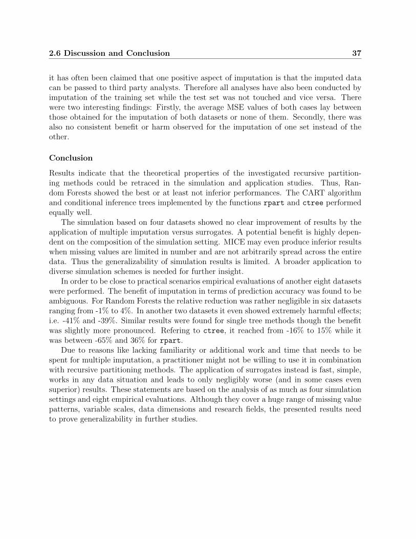
2.6 Discussion and Conclusion 37
it has often been claimed that one positive aspect of imputation is that the imputed datacan be passed to third party analysts. Therefore all analyses have also been conducted byimputation of the training set while the test set was not touched and vice versa. Therewere two interesting findings: Firstly, the average MSE values of both cases lay betweenthose obtained for the imputation of both datasets or none of them. Secondly, there wasalso no consistent benefit or harm observed for the imputation of one set instead of theother.
Conclusion
Results indicate that the theoretical properties of the investigated recursive partition-ing methods could be retraced in the simulation and application studies. Thus, Ran-dom Forests showed the best or at least not inferior performances. The CART algorithmand conditional inference trees implemented by the functions rpart and ctree performedequally well.
The simulation based on four datasets showed no clear improvement of results by theapplication of multiple imputation versus surrogates. A potential benefit is highly depen-dent on the composition of the simulation setting. MICE may even produce inferior resultswhen missing values are limited in number and are not arbitrarily spread across the entiredata. Thus the generalizability of simulation results is limited. A broader application todiverse simulation schemes is needed for further insight.
In order to be close to practical scenarios empirical evaluations of another eight datasetswere performed. The benefit of imputation in terms of prediction accuracy was found to beambiguous. For Random Forests the relative reduction was rather negligible in six datasetsranging from -1% to 4%. In another two datasets it even showed extremely harmful effects;i.e. -41% and -39%. Similar results were found for single tree methods though the benefitwas slightly more pronounced. Refering to ctree, it reached from -16% to 15% while itwas between -65% and 36% for rpart.
Due to reasons like lacking familiarity or additional work and time that needs to bespent for multiple imputation, a practitioner might not be willing to use it in combinationwith recursive partitioning methods. The application of surrogates instead is fast, simple,works in any data situation and leads to only negligibly worse (and in some cases evensuperior) results. These statements are based on the analysis of as much as four simulationsettings and eight empirical evaluations. Although they cover a huge range of missing valuepatterns, variable scales, data dimensions and research fields, the presented results needto prove generalizability in further studies.

38 2. Predictive Accuracy for Data with Missing Values

Chapter 3
A new Variable Importance Measurefor Missing Data
3.1 Research Motivation and Contribution
A highly valued feature of Random Forests, which is in the main focus of this chapter, isthe assessment of a variable’s relevance by means of importance measures. Unfortunately,there is no suggestion on how to compute such measures in the presence of missing values.Existing methods can not be used as there are evident violations against their most basicprinciples if applied straightforward. Hence one of the most appreciated properties ofRandom Forests, namely its ability to handle missing values, gets lost for the computationof importance measures. This chapter presents a solution to this pitfall by the introductionof a new variable importance measure that:
• retains the widely appreciated qualities of existing variable importance measures;
• is applicable to any kind of data, whether it does or does not contain missing values;
• is robust against different kinds of missing data generating processes;
• shows good variable ranking properties;
• meets sensible requirements;
• incorporates the full information provided by the entire data (i.e. without any needfor restrictions like complete case analysis);
• can deal with missing values in an intuitive and straightforward way.
The properties of the new method are investigated in an extensive simulation study. Twodata evaluations show the practicability of the new method in real life situations. Theyalso indicate that the new approach may provide a more sensible variable ranking than thewidespread complete case approach. The new proposal and corresponding investigationsof this chapter have been accepted for publication (Hapfelmeier et al., 2012b).

40 3. A new Variable Importance Measure for Missing Data
3.2 New Proposal
3.2.1 Definition
A new approach is suggested here in order to provide a straightforward and intuitive wayof dealing with missing values in the computation of a Random Forest variable importancemeasure. The construction of the new measure closely sticks to existing methodology whileit deviates from the original permutation accuracy importance (section 1.2.2) only in one– yet one substantial – step.
In the original permutation accuracy importance, the OOB values of a predictor variableof interested are randomly permuted to simulate the null-hypothesis H0 : Y,Z⊥Xj (cf.equation (1.3)). This mechanism destroys the relation of the predictor variable to theresponse and the remaining variable space. If the OOB accuracy drops substantially as aresult, the variable is termed to be of relevance. However, it is not clear how to proceedin the presence of missing values. In particular, it is not clear how conclusions about theimportance of a variable can be drawn from the permutation approach when surrogate splitsare used for the computation of the OOB accuracy but are not part of the permutationscheme. A simple extension of the permutation scheme to cover the surrogate variablesdoes not solve this issue but leads to additional undesirable effects; e.g. the importanceof all variables that are involved in the permutation would somehow be admixed. For thisproblem, a simple but efficient solution is suggested in the following.
The main idea of the new proposal is the following: Instead of permuting the OOBvalues of a variable (that may be missing), the corresponding observations are randomlyallocated to one of the child nodes if the split of their parent node is conducted in thevariable of interest. This procedure detaches any decision from the raw values of thevariable, and therefore circumvents any problems associated with the occurrence of missingvalues and the application of surrogate splits for the computation of the OOB accuracy.
The rest of the computation procedure, however, is not affected by this “trick”: In thefirst step of the computation one proceeds as normal by recording the OOB accuracy of atree (using all surrogate splits, which can be considered as an implicit imputation of themissing values). In a second step, the OOB accuracy is again recomputed by randomlyassigning OOB observations that were originally split in the variable of interest to thecorresponding child nodes.
Formally introducing a binary random variable D, that indicates the decision for oneof the child nodes, the probability of being sent to the left (D = 0) or to the right (D = 1)child node respectively is given by Pk(D = 0) and Pk(D = 1) = 1− Pk(D = 0) for a nodek. The random allocation of the OOB observations, just like the random permutation ofthe OOB values of a predictor variable Xj itself in the original permutation importance,mimics the null hypothesis that the assignment of observations to nodes does not dependon this particular predictor variable any more. Under the null-hypothesis, the probabilityto end up in a specific child node of node k is
Pk(D|Xj) = Pk(D).

3.2 New Proposal 41
Therefore it does not matter whether values of Xj are missing or not, as it is not used forthe decision of how to further process an observation.
For the practical computation of the prediction accuracy, the probability Pk(D = 0) isreplaced by its empirical estimator, the relative frequency:
pk(D = 0) = nk,left/nk
where nk,left and nk are the number of observations that were originally sent to the leftchild node and were present in parent node k, respectively. In contrast to the originalpermutation importance measure presented in section 1.2.2, the computation of the newmeasure consists of the following steps, highlighting the essential difference in step 2:
Compute the OOB accuracy of a tree.1.
Randomly assign each OOB observation with pk(D = 0) to thechild nodes of a node k that uses Xj for its primary split.2.
Recompute the OOB accuracy of the tree following step 2.3.
Compute the difference between the original and recomputed OOB accuracy.4.
Repeat step 1 to 4 for each tree.5.
The overall importance score is given by the average difference.6.
A corresponding implementation is given by the function varimp() in the R package partysince version 1.0-0.
3.2.2 Requirements
The characteristics of the proposed importance measure needed to be explored while italso had to follow some requirements. Therefore several properties were supposed to beclose to those of the original permutation importance measure like the fact that correlatedvariables obtain higher importances than uncorrelated ones in an unconditional assessment.Others were still to be investigated like the effect of different correlation structures (thatdetermine the quality and amount of surrogate variables), schemes of missingness, theamount of missing values and so forth.
In order to rate the performance of the newly suggested approach a list of requirementsthat should be met by a sensible variable importance measure designed for dealing withmissing values was formulated:
• (R1) When there are no missing values, the measure should provide the same variableimportance ranking as the original permutation importance measure.

42 3. A new Variable Importance Measure for Missing Data
• (R2) The importance of a variable is not supposed to artificially increase, but todecrease with an increasing amount of missing values (because the variable losesinformation, cf. Strobl et al., 2007a).
• (R3) Like the original permutation importance (that is a marginal importance in thesense of Strobl et al., 2008), the importance of a variable is supposed to increase withan increasing correlation to other influential predictor variables.
• (R4) The importance ranking of variables not containing missing values is supposedto stay unaffected by the amount of missing values in other variables. This is onlyrequired within groups of equally correlated variables as differences in correlationdirectly affect variable importances and therefore may well change the ranking.
• (R5) The importance of influential variables is supposed to be higher than the impor-tance of non-influential variables. This should hold for equally correlated variableswith equal amounts of missing values – considering that both facts influence the im-portance of a variable. For example a non-influential variable which does not containmissing values and is correlated with influential variables can achieve a higher impor-tance than an isolated influential variable containing missing values (cf. Strobl et al.,2008). In any case, the lowest importance should always be assigned to non-influentialvariables that are uncorrelated with any other influential variables.
In order to investigate these requirements and shed light on further characteristics of thenewly suggested approach, an extensive simulation study – as described in the followingsections – was set up.
3.3 Studies
3.3.1 Simulation Studies
There are several factors that need to be varied in the simulation setting, in particularthe amount of missing values, correlation strength, the number of correlated variables(termed block size in the following), variable influence and different missing data generatingprocesses. A detailed explanation of the setup is given in the following.
• Influence of predictor variables
The proposed importance measure is supposed to be applicable in both classificationand regression problems. Thus, the simulated data contained a categorical (binary)and a continuous response. In both cases the coefficients β, that were used to produce20 variables in the data generating model described below, are:
β = (4, 4, 3, 4, 3, 4, 3, 4, 3, 0, 0, 2, 2, 0, 0, 0, 0, 0, 0, 0)>

3.3 Studies 43
The idea of this setup was that a repeated choice of the same values for β enablesa direct comparison of importances of variables which are, by construction, equallyinfluential. The different β values are crossed with the other experimental factorsto allow an evaluation of differences and provide reference values for each setting.In addition, the non-influential variables with β = 0 help to investigate possibleundesired effects and serve as a baseline.
• Data generating models
A continuous response was modeled by means of a linear model:
y = x>β + ε with ε ∼ N(0, .5).
The binary response was drawn from a Bernoulli distribution B(1, π) while π wasassessed by means of a logistic model
π = P (Y = 1|X = x) =ex>β
1 + ex>β.
The variable set x itself contains 100 observations drawn from a multivariate normaldistribution with mean vector ~µ = 0 and covariance matrix Σ:
• Correlation
Σ =
1 r r 0 0 0 0 0 0 0 0 0 · · · 0r 1 r 0 0 0 0 0 0 0 0 0 · · · 0r r 1 0 0 0 0 0 0 0 0 0 · · · 00 0 0 1 r 0 0 0 0 0 0 0 · · · 00 0 0 r 1 0 0 0 0 0 0 0 · · · 00 0 0 0 0 1 r 0 0 0 0 0 · · · 00 0 0 0 0 r 1 0 0 0 0 0 · · · 00 0 0 0 0 0 0 1 r r r 0 · · · 00 0 0 0 0 0 0 r 1 r r 0 · · · 00 0 0 0 0 0 0 r r 1 r 0 · · · 00 0 0 0 0 0 0 r r r 1 0 · · · 00 0 0 0 0 0 0 0 0 0 0 1 · · · 0...
......
......
......
......
......
.... . . 0
0 0 0 0 0 0 0 0 0 0 0 0 0 1
As the variances of each variable are chosen to be 1, the covariance equals the corre-lation in this special case. The strength of correlation was varied by setting r to 0, .3,.6 and .9. The structure of the 20× 20 dimensional covariance matrix Σ reveals thatthere are four blocks of correlated variables of various sizes, each of them consistingof 3, 2, 2 and 4 variables, respectively. Thus it was possible to investigate the effectthat the strength and extent of the correlation had on the importance measure.

44 3. A new Variable Importance Measure for Missing Data
• Missing values
In analogy to the simulation setting of Rieger et al. (2010), who investigate theperformance of Random Forests on missing data, several MCAR and MAR schemeswere implemented to induce missing values. In addition, a further MNAR settingwas investigated. In each scheme, a given fraction m of observed values is replacedby missing values for selected variables. As the amount of missing values is of majorconcern in the simulation experiments, m takes the values 0%, 10%, 20% and 30%.
In a MAR setting, the probability for missing values in a variable depends on thevalues of another variable. In the MNAR scheme this probability is determined bya variables own values. Accordingly, each variable containing missing values has tobe linked to at least one other variable or itself. Table 3.1 lists the correspondingrelations.
contains missing values determines missing values(MCAR, MAR & MNAR) (MAR) (MNAR)X2 X3 X2
X4 X5 X4
X8 X9 X8
X10 X11 X10
X12 X13 X12
X14 X15 X14
Table 3.1: List of variables that contain missing values and variables that determine theprobability of a missing value.
The schemes to produce missing values are:
– MCAR: Values are randomly replaced by missing values.
– MAR(rank): The probability of a value to be replaced by a missing value riseswith the rank the same observation has in the determining variable.
– MAR(median): The probability of a value to be replaced by a missing value is 9times higher for observations whose value in the determining variable is locatedabove the corresponding median.
– MAR(upper): Those observations with the highest values of the determiningvariable are replaced by missing values.
– MAR(margins): Those observations with the highest and lowest values of thedetermining variable are replaced by missing values.
– MNAR(upper): The highest values of a variable are set missing.
The findings of Little and Rubin (2002) showed that usual sample estimates, forexample in linear regression, stay unaffected by the MCAR scheme. However, Strobl

3.3 Studies 45
et al. (2007a) outlined that in classification and regression trees even MCAR mayinduce a systematic bias, that may be carried forward to Random Forests based onbiased split selections. Therefore, in the following simulation study, one MCAR, fourMAR and one MNAR process to generate missing values are investigated to shedlight on the sensitivity of the proposed method to these schemes.
A schematic illustration of β summarizes all factors varied in the simulation design below.Correlated blocks of variables are enumerated by roman figures and separated by ’|’. Boldfigures indicate variables that contain missing values:
β = (4,4, 3︸ ︷︷ ︸I
| 4, 3︸︷︷︸II
| 4, 3︸︷︷︸III
|4, 3,0, 0︸ ︷︷ ︸IV
| 2︸︷︷︸V
| 2︸︷︷︸VI
| 0︸︷︷︸VII
| 0︸︷︷︸VIII
| 0︸︷︷︸IX
| 0︸︷︷︸X
| 0︸︷︷︸XI
| 0︸︷︷︸XII
| 0︸︷︷︸XIII
)>
In summary, there are 2 response types, 6 missing value generating processes, 4 fractionsof missing values and 4 correlation strengths, summing up to as much as 192 differentsimulation settings. Variable importances were recorded by repeating each setting 1000times. The corresponding R-Code is given in the appendix B.3.1.
3.3.2 Empirical Evaluation
In addition to the extensive simulation study, two well known data sets were used toshow the applicability of the new approach in real life situations. These are The PimaIndians Diabetes Dataset and the Mammal Sleep Data as presented in section 2.4.2. Bothwere chosen to provide a varying number of missing values in several variables. The totalnumber of variables equals 8 and 9 to allow for an easy and clear comparison of importancemeasures.
Besides the examination of the newly suggested approach, the original permutationimportance measure was applied, too. For the latter, the still popular complete caseanalysis approach was used, for which observations that contain missing values are entirelyomitted before the Random Forest is fit. Finally the ranking of variable importanceswithin each approach was compared and discussed. The corresponding R-Code is given inthe appendix B.3.2.
3.3.3 Implementation
The analyses of this chapter were again performed with the R system for statistical com-puting (R Development Core Team, 2011, version 2.14.1). The function cforest() of theparty package (Hothorn et al., 2008, version 1.0-0) was used as an unbiased implementa-tion of Random Forests. The settings for the simulation studies were chosen to result ina computation of ntree = 50 trees and maxsurrogate = 3 surrogate splits in each node.The number of randomly selected variables serving as candidates for splits was set to bemtry = 8. Sticking to the default setting mincriterion = 0 there were no restrictions con-cerning the significance of a split. Trees were grown until terminal nodes contained less than
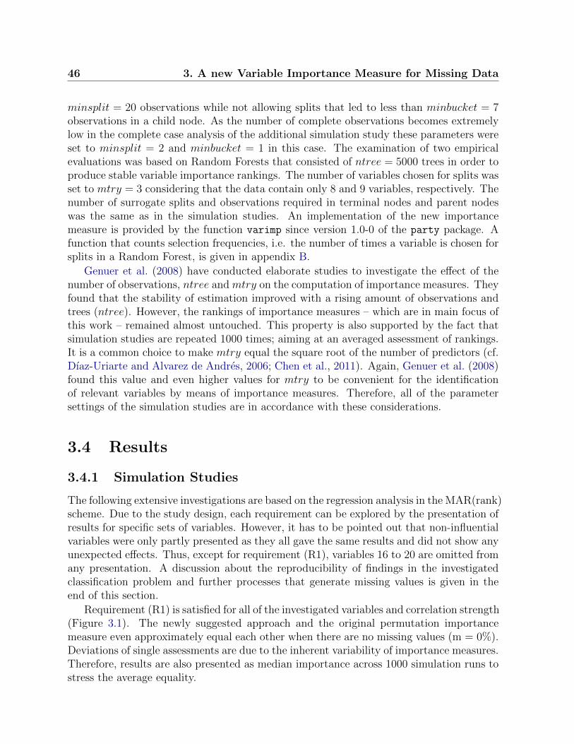
46 3. A new Variable Importance Measure for Missing Data
minsplit = 20 observations while not allowing splits that led to less than minbucket = 7observations in a child node. As the number of complete observations becomes extremelylow in the complete case analysis of the additional simulation study these parameters wereset to minsplit = 2 and minbucket = 1 in this case. The examination of two empiricalevaluations was based on Random Forests that consisted of ntree = 5000 trees in order toproduce stable variable importance rankings. The number of variables chosen for splits wasset to mtry = 3 considering that the data contain only 8 and 9 variables, respectively. Thenumber of surrogate splits and observations required in terminal nodes and parent nodeswas the same as in the simulation studies. An implementation of the new importancemeasure is provided by the function varimp since version 1.0-0 of the party package. Afunction that counts selection frequencies, i.e. the number of times a variable is chosen forsplits in a Random Forest, is given in appendix B.
Genuer et al. (2008) have conducted elaborate studies to investigate the effect of thenumber of observations, ntree and mtry on the computation of importance measures. Theyfound that the stability of estimation improved with a rising amount of observations andtrees (ntree). However, the rankings of importance measures – which are in main focus ofthis work – remained almost untouched. This property is also supported by the fact thatsimulation studies are repeated 1000 times; aiming at an averaged assessment of rankings.It is a common choice to make mtry equal the square root of the number of predictors (cf.Dıaz-Uriarte and Alvarez de Andres, 2006; Chen et al., 2011). Again, Genuer et al. (2008)found this value and even higher values for mtry to be convenient for the identificationof relevant variables by means of importance measures. Therefore, all of the parametersettings of the simulation studies are in accordance with these considerations.
3.4 Results
3.4.1 Simulation Studies
The following extensive investigations are based on the regression analysis in the MAR(rank)scheme. Due to the study design, each requirement can be explored by the presentation ofresults for specific sets of variables. However, it has to be pointed out that non-influentialvariables were only partly presented as they all gave the same results and did not show anyunexpected effects. Thus, except for requirement (R1), variables 16 to 20 are omitted fromany presentation. A discussion about the reproducibility of findings in the investigatedclassification problem and further processes that generate missing values is given in theend of this section.
Requirement (R1) is satisfied for all of the investigated variables and correlation strength(Figure 3.1). The newly suggested approach and the original permutation importancemeasure even approximately equal each other when there are no missing values (m = 0%).Deviations of single assessments are due to the inherent variability of importance measures.Therefore, results are also presented as median importance across 1000 simulation runs tostress the average equality.

3.4 Results 47
●
●
●
●●
●
●
●●
●
●●●
●●
● ●●
●●
●●
●
●●
●
●
●
●
●
●
●
●
●●●
●●●
●
●
●
●
●
●●●
●●
●●
●
●
●●
●
●●
●
●●●●●
●
●
●
●
●
●
●●●●
●●
●
●
●●
●●
●
●
●
●
●
●
●
●
●
●
●
●
●
●●
●●●●
●
●● ●
●●
●
●●
●
●
●
●
●
●●
●
●
●
●
●
●
●●
●
●
●●●●●
●
●
●
●
●●
●●●
●
●
●●●●●●●●
●
●
●●●
●●●● ●
●
●●
●
●
●
●●
●●
●
●●
●●●
●
●
●
●
●
●●●
●●
●
●
●●
●●●
●●
●
●●●● ●●
●
●
●
●●
●●●
●●
●
●
●
●●
●
●●
●●
●
●●
●
●
●●
●
●
●● ●
●
●●
●●●
●
●
●
●
●●●●
●●
●
●
●
●
●
●
●
● ●●●
●●
●
●●
●
●
●
●
●
●
●
●
●
●●
●
●
●
●
●●
●
●
●●●
● ●
●
●
●
●
●
●●
●
●
●
●
●
●
●
● ●
●
●
●
●
●●●
●●
●
●
●
●
●
●●●
●
●
●
●
●●●
●●
●
●
●●
● ●●
●●
●●●
●
●●●●●
●● ●
●●
●
●●
●●
●
●●
●
●
●
● ●
●
●
●●
●
●●
●●
●
●
●●●●
●●●
●●●
●●
●
●
●
●
●●
●●
●
●●●●
●
●● ●●
●
●●
●
●●
●
●
●
●●
●
●
●
●●
●●
●
●
●●●
●●
●
● ●
●
●
●
●
●
●
●●●
●
●
●
●●
●●●●
●
● ●
●
●●●
●
●
●
●
●
●
●
●
●
●●●
●
● ●
●
●
●
●●
●●●
●
●●
●
●●
●●
●
●●
●●
●
●●●
●●●
●
●
●
●●●● ●
●
●
●●
●
●●●
●
●●
●
●●
●●
●
●
●
●
●
●
●
●●●
● ●
●
●●
●
●
●
●
●●●
●
●
●
●
●●●
●
●
●●
●
●●●●●
●●
●●●●●●
●
●
●●●
●●
●●
●
●
●●
●
●
●
●
●
●
●
●●●
●
●●
●●
●
●
●
●
●●●●
●
●●
●●
●
●
●
●
●●
●●
●
●
●
●
●
●
●
●●●
●●●
●●
●●
●●
●●
●
●●
●
●
●
●●
●●
●
●
●
●
●●
●
●●●
●
●
●
●
●
●●●
●
●
●●
●
●●
●●●●
●
●●
●●
●
●●
●●●●
●
●
●
●●
●● ●●
●
●●
●
●
●●
●●●●●●
●●●
●
●
●●
●
●●
●●
●●
●
●
●
●●●
●
●
●
●
●
●●●
●
●●●●●
●●●●●●
●
●●
●●
●
●
●●
●
●
●
●
●●
●●●●
●●
●
●●●
●
●●
●●
●
●
●
●
●●
●
●●●●
●
●●●
●●
●
●
●
●●
●
●●
●
●●
●●
●
●●
● ●●●
●
●
●
●
●●
●
●
●
● ●●●
●
●●●●
●●
●
●
●
●
●
●
●
●
●●●
●
●●
●
●●●
●
● ●●
●●
●
●●●
●
●
●
●●
●
●●●●
●●
●●
●●
●●●●
●
●●
●●
●
●
●●
●
●
●●
●●
●
●●●●●●
●
●
●
●●●
●
●
●
●
●
●●
●●●
●
●
●
●
●
●
●●●●●●●
●
●●
●
●
●
●
●
●
●●
●
●●
●●
●
●
●
●●
●
●●●●●
●
●
●●●●
●
●
●●
●
●●
●
●
●
●
●●
●
●
●●
●●
●●
0 10 20 30 40 50 60 70
0
10
20
30
40
50
60
70
0 10 20 30 40 50 60 70
0
10
20
30
40
50
60
70
●●
●
●
●
●
●
●
●●●●●●●●●●●●
●●
●●●
●
●●
●●●●●●●●●●●●
●●
●
●●
●●
●●
●●●●●●●●●●●
●●
●
●●●●●●
●●●●●●●●●●●
New
App
roac
h
● ●● ●● ●● ● ●●● ●● ●● ●●●● ●●● ●● ●●●●● ●● ●● ●●●● ●●● ●●● ●●● ●● ● ●● ●●● ●●● ●●
●
●●●●
●
●●
●
●
●
●
●
●
●
●
●
●
●●
●
●●●
●●
●
●●
●●●
●
●
●
●●●●●
●
●
●
●●●
●
●
●●
●
●
●
●●
●●
●●
●
●
●
●
Original Permutation Importance
Figure 3.1: Comparison of the new approach and the original permutation importance.Left: Median importance measures across 1000 simulation runs for all variables and cor-relations when there is no missing data (m = 0%). Right: Distribution of values observedin 1000 simulation runs for the example of variable 5 (r = 0.6).
Requirement (R2) is met as the importance of variables decreases the more missingvalues they contain (Figure 3.2). This holds for all variables and correlation strengths(Figure A.1 in appendix A.2).
Requirement (R3) holds as correlations with influential variables induce higher impor-tances (Figure 3.3). This is true for all variables and fractions of missing values (FigureA.1 in appendix A.2; A comparison of blocks I and II shows that block size is anotherfactor that affects variable importance. However, non-influential variables, given in blockIV, do not contribute to this effect.).
The effects of correlation and missing values appear to be interacting (see block I inFigure 3.4): Although all variable importances rise with a rising strength of correlation,the importance of variable 2 drops in relation to the variables of the same block when the
Coef. = 4Block = IV
0% 10% 20% 30%m =
0
10
20
30
Var. 8
r =
.6
Coef. = 0Block = IV
0% 10% 20% 30%
Var. 10
Figure 3.2: Variable importance of variables 8 and 10 for a correlation of r = .6 and m =0%, 10%, 20%, 30% missing values. Boxplots of variables with missing values are coloredgrey. Outliers are omitted from illustration for clarity.

48 3. A new Variable Importance Measure for Missing Data
Var. 3
.0 .3 .6 .9r =
Coef. = 3Block = I
0
20
40
60
80
100
120
m =
30%
Var. 5
.0 .3 .6 .9
Coef. = 3Block = II
Var. 9
.0 .3 .6 .9
Coef. = 3Block = IV
Figure 3.3: Variable importances of variables 3, 5 and 9 for correlations of r = 0, .3, .6, .9.Outliers are omitted from illustration for clarity.
amount of missing values increases. An investigation of selection frequencies – i.e. thenumber of times a variable is chosen for splits in a Random Forest (displayed as horizontallines) – reveals that it is replaced by other variables in the tree building process. Thiseffect follows a simple rule: the more similar the information of variables becomes due toan increased correlation, and the more information a variable is lacking because of missingvalues, the more often it will be replaced by others.
Requirement (R4) is satisfied as the ranking of fully observed variables from the sameblock stays unaffected by the amount of missing values in other variables (Figure 3.4).Note that between blocks the variable rankings may change: The importance of variable5 increases as it is able to replace variable 4 that contains missing values. It rises abovevariable 7 with the same (and for strong correlations and many missing values even abovevariable 6 with a higher) influence on the response. Another question emerging from thefact that variables may replace others in a tree is if this also holds for isolated blocksthat are not correlated with any variables that contain missing values. Figure 3.5 showsthat this is almost not the case as selection frequencies and variable importances stay ona certain level for block III compared to block II). This finding even partly extends (R4)which demands stable rankings for fully observed variables only within blocks, not acrossblocks.
Requirement (R5) is met as the importance of influential variables is higher than fornon-influential variables (Figure 3.6). This holds for variables with and without missingvalues, but not necessarily for comparisons between the two cases. Importances of influ-ential variables may drop below those of non-influential ones if the former contain missingvalues and the latter are part of a correlated block with influential variables. An example isgiven by block IV: Variable 8 shows a higher importance than variable 10 (both containingmissing values) and variable 9 shows a higher importance than variable 11 (both withoutmissing values). However, the importance of the influential variable 8 drops below thatof the non-influential variable 11, as the former contains missing values and the latter iscorrelated to variable 9. The importance of variable 11 even rises above that of influentialvariables contained in other blocks (e.g. variable 13). However, the lowest importance

3.4 Results 49
020406080
100120
m = 0%
r =
.0
0
20
39
58
78
m = 30%
4 4 3 4 3 4 3Coef.
1 2 3 4 5 6 7Var.
I I I II II III IIIBlock
020406080
100120
r =
.9
4 4 3 4 3 4 31 2 3 4 5 6 7I I I II II III III
0
20
39
58
78
Figure 3.4: Variable importances (left axis) of variables 1–7 (Block I, II, III) for correlationsof r = 0, .9 and fractions of missing values m = 0%, 30%. Boxplots of variables that containmissing values are colored grey. Horizontal lines indicate selection frequencies (right axis).Vertical dashed lines indicate correspondance to the same block. Outliers are omitted fromillustration for clarity.
0
10
20
30
40
m = 0%
r =
.6
0
15
30
44
59
m = 30%
4 3 4 3Coef.
4 5 6 7Var.
II II III IIIBlock
0
10
20
30
40
r =
.9
4 3 4 34 5 6 7II II III III
0
15
30
44
59
Figure 3.5: Variable importances (left axis) of variables 4–7 (Blocks II, III) for correlationsof r = .6, .9 and fractions of missing values m = 0%, 30%. Boxplots of variables that containmissing values are colored grey. Horizontal lines indicate selection frequencies (right axis).Vertical dashed lines indicate correspondance to the same block. Outliers are omitted fromillustration for clarity.

50 3. A new Variable Importance Measure for Missing Data
0
10
20
30
40
m = 20%
r =
.6
m = 30%
4 3 0 0 2 2 0 0Coef.
8 9 10 11 12 13 14 15Var.
IV IV IV IV V VI VII VIIIBlock
0
10
20
30
40
r =
.9
4 3 0 0 2 2 0 08 9 10 11 12 13 14 15IV IV IV IV V VI VII VIII
Figure 3.6: Variable importances of block IV–VIII for correlations of r = .6, .9 and fractionsof missing values m = 20%, 30%. Boxplots of variables that contain missing values arecolored grey. Vertical dashed lines indicate correspondance to the same block. Outliers areomitted from illustration for clarity.
should always be assigned to non-influential variables that are uncorrelated with any otherinfluential variables. This claim is supported by the examples of variable 14 and 15.
In conclusion, factors like the occurrence of missing values, the number and influence ofcorrelated variables as well as the correlation strength, can positively affect the importanceof variables. However, these are properties to be expected from a marginal variable im-portance measure when dealing with variables that lose information due to missing values,yet are correlated to other variables that can “take over for them”.
Results of the entire simulation setting for the regression problem are displayed in Figure3.7 for a broad overview. The results show the same properties that were already pointedout for the specific settings above. An additional comparison of results for all schemes usedto produce missing values (MCAR, MAR(rank), MAR(median), MAR(upper), MAR(mar-gins) and MNAR(upper)) is given by Figure 3.8. For the purpose of clarity it concentrateson the case of r = .6 and m = 20%. None of the schemes shows any noticeable differences;all findings of the previous analyses in the MAR(rank) setting can be retraced in eachscheme. In conclusion, the proposed approach shows the same properties for a wide rangeof MCAR, MAR and MNAR missing data schemes. Likewise, results for the classificationproblem show the same properties (Figure A.3 in the appendix A.2) and thus are notdiscussed in detail to omit redundancy.
3.4.2 Empirical Evaluation
Figure 3.9 shows the results observed for the two data evaluations. Both datasets were an-alyzed in two ways: By applying the new approach to the full data set and by applying the

3.4 Results 51
0
20
40
60
80
100
120
m = 0%
r =
.0
m = 10% m = 20%
0
20
39
58
78
m = 30%
0
20
40
60
80
100
120
r =
.3
0
20
39
58
78
0
20
40
60
80
100
120
r =
.6
0
20
39
58
78
4 4 3 4 3 4 3 4 3 0 0 2 2 0 0Coef.1 2 3 4 5 6 7 8 9 10 11 12 13 14 15Var.I I I II II III III IV IV IV IV V VI VII VIIIBlock
0
20
40
60
80
100
120
r =
.9
4 4 3 4 3 4 3 4 3 0 0 2 2 0 01 2 3 4 5 6 7 8 9 10 11 12 13 14 15I I I II II III III IV IV IV IV V VI VII VIII
4 4 3 4 3 4 3 4 3 0 0 2 2 0 01 2 3 4 5 6 7 8 9 10 11 12 13 14 15I I I II II III III IV IV IV IV V VI VII VIII
4 4 3 4 3 4 3 4 3 0 0 2 2 0 01 2 3 4 5 6 7 8 9 10 11 12 13 14 15I I I II II III III IV IV IV IV V VI VII VIII
0
20
39
58
78
Figure 3.7: Variable importances (left axis) of block I–VIII for correlations of r = 0, .3, .6,.9 and fractions of missing values m = 0%, 10%, 20%, 30% in the MAR(rank) setting ofthe regression problem. Boxplots of variables that contain missing values are colored grey.Horizontal lines indicate selection frequencies (right axis). Vertical dashed lines indicatecorrespondance to the same block. Outliers are omitted from illustration for clarity.

52 3. A new Variable Importance Measure for Missing Data
4 4 3 4 3 4 3 4 3 0 0 2 2 0 0Coef.
1 2 3 4 5 6 7 8 9 10 11 12 13 14 15Var.
I I I II II III III IV IV IV IV V VI VII VIIIBlock
0
20
40
60
80
100
0
17
34
50
67
m = 20%
r =
.6
(a) MCAR
4 4 3 4 3 4 3 4 3 0 0 2 2 0 0Coef.
1 2 3 4 5 6 7 8 9 10 11 12 13 14 15Var.
I I I II II III III IV IV IV IV V VI VII VIIIBlock
0
20
40
60
80
0
18
36
55
73
m = 20%
r =
.6
(b) MAR(rank)
4 4 3 4 3 4 3 4 3 0 0 2 2 0 0Coef.
1 2 3 4 5 6 7 8 9 10 11 12 13 14 15Var.
I I I II II III III IV IV IV IV V VI VII VIIIBlock
0
20
40
60
80
100
0
20
40
60
80
m = 20%
r =
.6
(c) MAR(median)
4 4 3 4 3 4 3 4 3 0 0 2 2 0 0Coef.
1 2 3 4 5 6 7 8 9 10 11 12 13 14 15Var.
I I I II II III III IV IV IV IV V VI VII VIIIBlock
0
20
40
60
80
100
0
18
36
55
73
m = 20%
r =
.6
(d) MAR(upper)
4 4 3 4 3 4 3 4 3 0 0 2 2 0 0Coef.
1 2 3 4 5 6 7 8 9 10 11 12 13 14 15Var.
I I I II II III III IV IV IV IV V VI VII VIIIBlock
0
20
40
60
80
100
0
18
35
52
70
m = 20%
r =
.6
(e) MAR(margins)
4 4 3 4 3 4 3 4 3 0 0 2 2 0 0Coef.
1 2 3 4 5 6 7 8 9 10 11 12 13 14 15Var.
I I I II II III III IV IV IV IV V VI VII VIIIBlock
0
20
40
60
80
100
0
17
34
52
69
m = 20%
r =
.6
(f) MNAR(upper)
Figure 3.8: Variable importances (left axis) of variables 1–15 for a correlation of r = .6and a fraction of missing values m = 20% in the regression problem. Boxplots of variablesthat contain missing values are colored grey. Horizontal lines indicate selection frequencies(right axis). Vertical dashed lines indicate correspondance to the same block. Outliers areomitted from illustration for clarity.

3.4 Results 53
num.preg gluc bloodpres skin insulin bmi pedigree age
Original Perm. Imp.New Approach
Pima Indian Diabetes
0
0.03
0.06
0.09
0
0.03
0.06
0.09
4
8
1 2
65 3
7
5
8
1 2 3
7
46
0% 0.7% 4.6% 29.6% 48.7% 1.4% 0% 0%m =
BrainWgt NonD Dream Sleep Span Gest Pred Exp Danger
Mammal Sleep
0
2500
5000
7500
0
21000
42000
630009
6
1
4
5
8
2
7
3
9
5
34 6
8
2
7
1
0% 22.6% 19.4% 6.5% 6.5% 6.5% 0% 0% 0%m =
Figure 3.9: Variable Importances for the Pima Indians and the Mammal Sleep Data. Blackand grey bars correspond to the original permutation importance measure (complete caseanalysis; left axis) and the new approach (right axis), respectively. Heights of bars werematched in relation to the maximally observed importance of each approach. Figures abovebars indicate ranks within methods. The fraction of missing values per variable is givenby m.
original permutation importance measure in a complete case analysis, where observationswith missing values are excluded from analysis.
In the Pima Indians Diabetes Data the ranking of predictor variables shows severe dif-ferences between methods: The new approach assigns a higher importance to the variablesBMI, number of pregnancies and the diabetes pedigree function. It downgrades the vari-ables age and 2-Hour serum insulin. The strongest and weakest variables, however, plasmaglucose concentration, diastolic blood pressure and triceps skin fold thickness are rankedequally. Similar findings can be observed for the Mammal Sleep Data. The variables slowwave sleep (‘NonD’ = ‘nondreaming’), dreaming sleep, maximum life span and the overalldanger index are ranked differently.
A plausible reason for these differences is that complete case analysis can induce a biaswhen observations are not MCAR. This is well-known, yet complete case analysis is still fre-

54 3. A new Variable Importance Measure for Missing Data
quently applied in practice. Results show that differences do not directly (or solely) dependon whether or not a variable contains missing values. Complete case analysis can modifythe entire importance ranking just because information is omitted when observations areexcluded from the analysis.
To illustrate one possible scenario that can lead to a change in the variable ranking whencomplete case analysis is applied to data that is not MCAR, another small simulation wasconducted. Given a pair of binary variables (U, V ) the response Y follows the distribution:
Y ∼
N(2, 1) if (u, v) = (1, 0)
N(0, 1) if (u, v) = (0, 0) or (u, v) = (1, 1)
N(−2, 1) if (u, v) = (0, 1)
The relative frequencies of class 0 and class 1 in U and V are 80% and 20%, respectively.They are not correlated. Missing values are induced into V dependent on the highest valuesof Y which resembles the MAR(upper) scheme. To produce stable results the simulationis based on 5,000 observations and Random Forests growing 5,000 trees. According to ourexpectation Figure 3.10a displays the same importance for both variables when there areno missing values in the data. In Figure 3.10b a fraction of 30% of V is set missing. Thenew approach is able to incorporate the entire data into the computation of the importancemeasures and assigns a reduced importance to V while U remains of high relevance. Thisfinding again meets our expectations. In a complete case analysis however, U suffers theloss of its explanatory power although it does not contain any missing values at all. It isnot even correlated to V. The explanation of this effect is quite simple: The highest valuesof Y which cause the missing values in V are most frequently related to u = 1. Deletingthese observations in a complete case analysis makes U mainly consist of class 0. As aconsequence it loses its discriminatory power. This example demonstrates how a completecase analysis can distort the ranking of variable importances when the missingness schemeis not MCAR. The new approach follows a much more sensible way of producing importancemeasures in any situation. Corresponding, more elaborate investigations of this issue aregiven in the following chapters 4 and 6.
3.5 Discussion and Conclusion
In summary, the simulation results have shown that all requirements that were previouslyformulated were fulfilled by the newly suggested importance measure for different types ofMCAR, MAR and MNAR missing data. Most importantly: In the absence of missing val-ues, both the original permutation importance measure and the newly suggested approachproduce similar results. The importance of variables containing missing values does notartificially increase but decreases with the number of missing values and the respectivedecrease of information. Moreover, in the presence of correlation, the measure shows allproperties that are to be expected from a marginal variable importance measure.
A particularly interesting effect is that with regard to the variable selection frequen-cies, variables with increasing numbers of missing values are increasingly replaced by fully

3.5 Discussion and Conclusion 55
U V
0.0
0.2
0.4
0.6
0.8
1.0
1.2
(a) No missing values
U V
0
0.31
0.62
0.93
0
0.44
0.87
1.31
Original Perm. Imp.New Approach
(b) 30% missing values in V
Figure 3.10: Variable importances of U and V computed by the original permutationimportance measure (black bars; left axes) and the new approach (grey bars; right axis).Case (a) is based on the entire data without any missing values. In case (b) 30% of variableV are set missing. A complete case analysis is used to compute the original permutationimportance (black) while the new approach is able to process the entire data (grey).
observed variables that are correlated with them: the complete variables “take over” forthose with missing values within a group of correlated ones. Similar findings about the’...competition of correlated variables for selection into a tree...’ have already been outlinedby Nicodemus et al. (2010). In this sense, the effects of correlation and missing values areinteracting. This is an intuitive property, since both affect the amount of information avariable retains.
What is important to note here is that, besides effects of the correlation on the permu-tation importance that were already pointed out by Strobl et al. (2008), in the presenceof missing values the correlation is also linked to the quality of surrogate variables. Theexact role that surrogate variables play for the variable importance is still ambiguous: Onone hand they help to reconstitute missing information, but on the other hand they alsocompete for the selection in the tree. However, the selection frequencies displayed in theresults indicate that the latter effect is stronger.
Besides the findings for the simulation analysis the new approach also appears wellsuited to deal with missing values in the evaluation study: There were some profounddifferences between the variable ranking suggested by the new approach and a completecase analysis. As the latter is known to produce biased results in many situations (e.g.,Janssen et al., 2009, 2010) this strongly indicates that the omission of observations withmissing values has induced artifacts because the values were not missing at random. Resultsof corresponding simulation studies support this claim.
The advantage of the new approach proposed in this work is that it incorporates the fullinformation provided by the data. Moreover, it reconstitutes one of the most appreciatedproperties of recursive partitioning methods, namely their ability to deal with missingvalues. The rationale of the approach is not to undo the influence missing values have onthe information carried by a variable, but to reflect the remaining information that the

56 3. A new Variable Importance Measure for Missing Data
variable retains with the respective values missing. Accordingly, the resulting importancerankings do not only depend on the amount of missing values but also on the quality andavailability of surrogate variables.

Chapter 4
Variable Importance with MissingData
4.1 Research Motivation and Contribution
A new variable importance measure that is able to deal with missing values has been intro-duced in chapter 3. However, there are also alternative solutions like imputation methodsand complete case analysis that enable the computation of the permutation importancemeasure in such cases. Therefore an extensive simulation study, that involves variousmissing data generating processes, is conducted in this chapter to explore and compare theability of
• complete case analysis,
• multiple imputation and
• the new importance measure
to produce reliable estimates of a variable’s relevance. Both, regression and classificationproblems are explored. In addition, the predictive accuracy of Random Forests that arebased on each of these approaches is investigated for a simulated test dataset. The latterissue has already been explored in chapter 2: comparisons of models fit with and withoutimputation of missing values showed only negligible differences. By contrast, the followingstudy focuses on the assessment of a variables importance measure. As a result the abilityto produce reliable estimates differs between approaches. Findings and recommendations:Complete case analysis should not be applied as it may inappropriately penalize variablesthat were completely observed. The new importance measure is much more capable ofreflecting decreased information exclusively for variables with missing values and shouldtherefore be used to evaluate actual data situations. By contrast, multiple imputationallows for an estimation of importances one would potentially observe in complete datasituations. The investigations of this chapter have been published as a technical report inHapfelmeier et al. (2012a).

58 4. Variable Importance with Missing Data
4.2 Simulation Studies
There are several factors of potential influence that needed to be explored in the simulationstudy. Therefore the amount of missing values, correlation schemes, variable strength anddifferent processes to generate missing values were of particular interest. The setup closelyresembles the one given in section 3.3.1. However, there are essential differences as listedin the following:
• Influence of predictor variables
The simulated data again contained both, a classification and a regression problem.Therefore, a categorical (binary) and a continuous response were created in depen-dence of six variables with coefficients β:
β = (1, 1, 0, 0, 1, 0)>.
Repeated values for β make it possible to compare importances of variables whichare, by construction, equally influential but show different correlations and differentfractions of missing values. In addition, the non-influential variables with β = 0 helpto investigate possible undesired effects and serve as a baseline.
• Correlation
Σ =
1 0.3 0.3 0.3 0 0
0.3 1 0.3 0.3 0 00.3 0.3 1 0.3 0 00.3 0.3 0.3 1 0 0
0 0 0 0 1 00 0 0 0 0 1
As the variances of each variable are chosen to be 1, the covariance equals the cor-relation in this special case. The structure of the covariance matrix Σ reveals thatthere is a block of four correlated variables and two uncorrelated ones.
• Missing values
Several MCAR, MAR and MNAR processes to create missing values were imple-mented. For each scheme, a given fraction m ∈ {0.0, 0.1, 0.2, 0.3} of values is set miss-ing for the variables X2, X4 and X5 (cf. Table 4.1). The number of observations thatcontain at least one missing value is given by 1−(1−%missing)nvariables . Thus, a datasetthat contains three variables with 30% missing values includes 1− (1−0.3)3 = 65.7%incomplete observations on average. This seems to be a rather huge amount rarelyseen for real life data. Nevertheless, this way m comprises a wide range of pos-sible scenarios. The schemes to produce missing values were MCAR, MAR(rank),MAR(median), MAR(upper), MAR(margins) and MNAR(upper).

4.3 Results 59
contains missing values determines missing values(MCAR, MAR & MNAR) (MAR) (MNAR)X2 X1 X2
X4 X2 X4
X5 X6 X5
Table 4.1: List of variables that contain missing values and determine the probability ofmissing values.
• Validation
An independent test dataset served the purpose to evaluate the predictive accuracyof a Random Forest. It was created the same way as the training data thoughit contained 5000 observations and was completely observed. The accuracy wasassessed by the mean squared error (MSE) which equals the misclassification errorrate (MER) in classification problems.
• Implementation
The implementation of the simulation was similar to the one described in section3.3.3: The function cforest() of the party package (Hothorn et al., 2008, ver-sion 1.0-0) was used with settings ntree = 50, mtry = 3, maxsurrogate = 3,mincriterion = 0, minsplit = 20 and minbucket = 7. MICE was again appliedby the function mice() of the mice package (van Buuren and Groothuis-Oudshoorn,2010, version 2.11) to produce five imputed datasets with defaultMethod = c(”norm”,”logreg”, ”polyreg”). Corresponding R-Code is given in section B.4.
In summary, there were 2 response types investigated for 6 processes to generate and 3procedures to handle 4 different fractions of missing values. This sums up to 144 simulationsettings. The simulation was repeated 1000 times.
4.3 Results
The following investigations are based on the classification analysis. Results for the regres-sion problem are presented as supplementary material in section A.3 (Figure A.4) as theyshowed similar properties.
A general finding which holds for each analysis accentuates the well-known fact thatunconditional permutation importance measures rate the relevance of correlated variableshigher than that of uncorrelated ones with the same coefficients (Strobl et al., 2008).This becomes evident by the example of variables 1, 2 and 5. Although they are of equalstrength the latter is assigned a lower relevance as it is uncorrelated to any other predictor;in some research fields this effect is appreciated to uncover relations and interactions amongvariables (cf. Nicodemus et al., 2010; Altmann et al., 2010). Also, there were no artificialeffects observed for the non-influential variable 6 in any analysis setting.

60 4. Variable Importance with Missing Data
MCAR
0.000.010.020.030.040.050.06 MAR(rank)
m = 0.0 0.1 0.2 0.3
MAR(median)
MAR(upper)
0.000.010.020.030.040.050.06
2 2 0 0 2 01 2 3 4 5 6
Coef.Var.
MAR(margins)
2 2 0 0 2 01 2 3 4 5 6
MNAR(upper)
2 2 0 0 2 01 2 3 4 5 6
impo
rtan
ce
Figure 4.1: Median variable importance observed for the new importance measure in theclassification problem (m = % of missing values in X2, X4 and X5).
Findings for the new variable importance measure which is able to implicitly deal withmissing values are displayed by Figure 4.1. According to expectations, the importance ofvariables 2, 4 and 5 decreased as they contained a rising amount of missing values. Itis interesting to note that meanwhile the importance of variable 1 rose, although it doesnot seem to be directly affected. However, the findings of chapter 3 showed that thisgain of relevance is justified: variables that are correlated and therefore provide similarinformation replace each other in a Random Forest when some of the information gets lostdue to missing values. Accordingly, variable 1 takes over for variable 2 which results in anincreased selection frequency of variable 1 in the tree building process. In conclusion, thisapproach is allowed to be affected by the occurrence of missing values as it mirrors thesituation at hand, i.e. the relevance a variable takes in a Random Forest considering of theinformation it actually provides. The new importance measure appeared to be well suitedfor any of the missing data generating processes as results did not differ substantially.
Results for the complete case analysis – given by Figure 4.2 – showed undesired effects.A rising amount of missing values lead to a decreased importance of the completely ob-served variable 1. This might partly be explained by the general loss of information assome observations are discarded from analysis. However, the importance of variable 1 isnot supposed to drop below that of variable 2 which is of equal strength yet contains themissing values. Unfortunately, this latter effect can be observed for every missing datagenerating process, except for MNAR(upper). It is most pronounced for MAR(upper) andMAR(margins). There is no rational justification for this property as variable 1 actuallyretains its information while other variables lose it. A proper evaluation of a variable’srelevance is supposed to reflect this fact. Considering this vulnerability of complete caseanalysis to different missing data generating processes it should not be used for the assess-ment of importance measures when there are missing data.

4.3 Results 61
MCAR
0.000.010.020.030.040.050.06 MAR(rank)
m = 0.0 0.1 0.2 0.3
MAR(median)
MAR(upper)
0.000.010.020.030.040.050.06
2 2 0 0 2 01 2 3 4 5 6
Coef.Var.
MAR(margins)
2 2 0 0 2 01 2 3 4 5 6
MNAR(upper)
2 2 0 0 2 01 2 3 4 5 6
impo
rtan
ce
Figure 4.2: Median variable importance observed for the complete case analysis in theclassification problem (m = % of missing values in X2, X4 and X5).
An examination of Figure 4.3 reveals that multiple imputation, with as few as fiveimputed data sets, is a convenient way to maintain and recover the importance of variablesthat would have been observed if there were no missing data at all. This equally held forvariables that contained missing values and those which were completely observed; none oftheir importances was arbitrarily decreased or increased. Even the importance of variable5, which is only related to the outcome and therefore is associated with a rather weakimputation model, remained unaffected by the amount of missing values. The example ofvariable 4 shows that the imputation of non-influential variables did not induce artificialimportances. All missing data generating processes showed these advantageous properties,except for the MNAR(upper) setting.
The prediction error produced by each approach for the independent test sample isdisplayed in Figure 4.4. For multiple imputation the prediction accuracy only slightly de-creases with a rising amount of missing values. This effect is more pronounced for RandomForests that use surrogate splits; though there are only minor differences to multiple im-putation (Rieger et al., 2010; Hapfelmeier et al., 2011, for similar findings). Complete caseanalysis appears to be much worse and leads to very high errors with a rising fraction ofmissing values. Missing data generating processes give comparable results within each ap-proach. However, there is one exception for the MNAR setting that always causes the worstresults. A corresponding evaluation of the regression problem is given as supplementarymaterial in section A.3 (Figure A.5).

62 4. Variable Importance with Missing Data
MCAR
0.000.010.020.030.040.050.06 MAR(rank)
m = 0.0 0.1 0.2 0.3
MAR(median)
MAR(upper)
0.000.010.020.030.040.050.06
2 2 0 0 2 01 2 3 4 5 6
Coef.Var.
MAR(margins)
2 2 0 0 2 01 2 3 4 5 6
MNAR(upper)
2 2 0 0 2 01 2 3 4 5 6
impo
rtan
ce
Figure 4.3: Median variable importance observed for the imputed data in the classificationproblem (m = % of missing values in X2, X4 and X5).
4.4 Conclusion
The ability of a new importance measure, complete case analysis and a multiple impu-tation approach to produce reasonable estimates for a variable’s importance in RandomForests has been investigated for data that contain missing values. Therefore, an extensivesimulation study that employed several MCAR, MAR and MNAR processes to generatemissing values has been conducted. There are some clear recommendations for application:Inappropriate results have been found for the complete case analysis in the MAR settings;it penalized the importance of variables that were completely observed in an arbitrary way.As a consequence, the sequence of importances was not able to reflect the true relevanceof variables any more. This approach is not recommended for application. By contrast thenew importance measure was able to express the loss of information exclusively for vari-ables that contained missing values. Therefore, it should be used to describe the relevanceof a variable under consideration of its actual information. In some cases one might preferto investigate the relevance a variable would have taken if there had been no missing val-ues. Multiple imputation appeared to serve this purpose very well except for the MNARsetting. An additional evaluation of prediction accuracy revealed that Random Forestsbased on multiple imputed data were mostly unaffected by the occurrence of missing val-ues. Results were only slightly worse when surrogate splits were used to process missingvalues. Complete case analysis lead to models with the lowest prediction strength.

4.4 Conclusion 63
●●●●
●
●
●●●●●●●● ●
●●●
●
●
●
●●●●●●● ●●
●●
●
●
●●●●
●
●
● ●
●●
●
●
●●
●●
●●●●
●
●
●
●
●●●●● ●
●●●
●
●●●
●●●
●
●
●
●●●●●
●
●●
●●●●
●●●●●●●●●
●●● ●
●●●
●
●
●
●
●●●●●
●●
●
●●
●
●●●●●
●
●●
●●
●●
●●
●
●●
●
●●●●
●
●
●
●
●
●
●
●
●
●
●
●
●●
●
●
●●
●
●
●
●
●
●●●●●●●●●●●●●●●●●●●●●●●●●●●●●●●●●●●●●●●●●●●●●●●●●●●●●●●●●●●●●●●●●●●●●●●●●●●●●●●●●●●●●●●●●●●●●●●●●●●●●●●
0.25
0.3
0.35
0.4
0.45MCAR
new measure complete caseimputation
●●●●
●
●
●●●●●●●●
●●
●
●●●●●●●●
●●●●●●
●●
●●●
●
●●
●
●●
●
●●●
●
●
●●●●
●
●
●
●
●●●●● ●●●
●
●
●
●●●
●
●●● ●
●
●●●●●●●●
●●
●●●●●●●●●●●●●●●
●●● ●
●●●
●
●
●
●
●●●●●
●●●●●●
●
●
●
●●
●●
●
●●
●
●
●
●
●
●
●●●●●
●●
●
●
●
●
●
●
●●
●
●
●
●
●
●
●
●
●
●●
●●
●
●●
●
●●●●●●●●●●●●●●●●●●●●●●●●●●●●●●●●●●●●●●●●●●●●●●●●●●●●●●●●●●●●●●●●●●●●●●●●●●●●●●●●●●●●●●●●●●●●●●●●●●●●
0.25
0.3
0.35
0.4
0.45MAR(rank)
●●●●
●
●
●●●●●●●●
●●●●
●
●●●●
●●
●
●
●●●
●
●
●●●
●●●●●●●
●
●
●●●●
●
●
●
●
●●●●● ●
●●
●
●●●●● ●
●●●●●
●●●●●●●
●
●●●
●
●●●●
●●●●
●
●
●
●
●●●●●
●●
●
●
●
●●●●
●
●
●
●●●
●
●
●
●
●
●
●●
●
●
●
●
●●●●●
●
●
●
●
●
●
●
●
●
●
●
●
●
●
●●
●
●
●
●
●
●●●●
●●
●
●
0.25
0.3
0.35
0.4
0.45MAR(median)
●●●●
●
●
●●●●●●●●
●
●
●
●
●
●●●
●●●●●●●●●●
●
●
●●●
●
●●●●
●
●
●●●●
●●●●
●
●
●
●
●●●●● ●
●●
●●
●
●
●●●●
●
●●●●●●
●
●●
●
●●
●●●●
●
●●●●
●●
●
●●●●●●
●
●●●●
●
●
●
●
●●●●●
●●
●
●●
●●●●●
●
●
●
●
●
●
●
●
●●
●
●
●
●●
●
●
●
●●
●●
●●
●●
●
●●●
●
●
●●
●
●●
●
●
●
●
●
●
●
●
●
●
●
●●
●
●
●
●
●●
●
●●
●
●
●●
●
●
●●
0.25
0.3
0.35
0.4
0.45MAR(upper)
●●●●
●
●
●●●●●●●●
●●●
●●
●
●●●●●
●
●●●●
●
●●
●●
●●●●
●
●
●●●●●●
●●●●●●●●●●●
●
●●●●
●
●
●
●
●●●●●
●●●
●
●●●
●
●●●● ●●●●
●
●●●●●
●
●●●
●
●●●●
●
●●●
●
●
●●●●●
●
●●●●
●
●
●
●
●●●●●
●
●
●
●
●
●
●●●●●●●●
●
●●
●
●●●
●
●
●
●
●
●●●
●
●
●●
●
●
●
●●
●●
●
●
●●●
●
●●
●●●
●
●●
●
●
●
●
0.25
0.3
0.35
0.4
0.45MAR(margins)
●●●●
●
●
●●●●●●●●
●●●●
●●
●
●
●●●●●●●●
●●
●
●●●●
●
●●●●
●
●●●●
●●●●●●●●●
●
●
●●
●●●●
●
●
●
●
●●●●● ●●●
●
●●●●●●●●●●
●●
●
●●●●
●
●●●●
●
●●
●●●●
●●
●
●●●●●
●
●●
●●●●
●
●
●
●
●●●●●
●
●
●●
●
●●
●
●●
●
●
●
●
●
●●
●●
●
●
●
●●
●
●
●
●●
●●
●
●●
●
●
●
●●●●●●●
●●●●●●●●●●●●●●●
●
●●●●●●●
●
●●●
●
●●●●●●●●●●
●
●●●●●●●●●●
●●●●●●
●●●●●●●●●●●●
●
0.25
0.3
0.35
0.4
0.45MNAR(upper)
.0 .1 .2 .3 .0 .1 .2 .3 .0 .1 .2 .3m =
MS
E
Figure 4.4: MSE observed for the classification problem (m = % of missing values in X2,X4 and X5).

64 4. Variable Importance with Missing Data

Chapter 5
A new Variable Selection Method
5.1 Research Motivation and Contribution
The application of variable selection mainly pursues two objectives: an improved predic-tion accuracy and the identification of relevant variables. Several approaches for variableselection have been proposed to combine and intensify these qualities (e.g. Dıaz-Uriarteand Alvarez de Andres, 2006; Rodenburg et al., 2008; Sandri and Zuccolotto, 2006; Tanget al., 2009; Yang and Gu, 2009); a summary of various selection methods and related pub-lications is provided by Archer and Kimes (2008). However, the definition of the expression‘relevance’ is strongly influenced by the research field the analytical question emerges from.For example, in the field of genome-wide association studies (GWAS) or microarray anal-ysis, variable selection is used to uncover noticeable expression levels, influential genesand genes which are functionally related to the latter. Following this definition, variableswhich themselves are informative and variables which are non-informative but correlatedto informative ones are termed to be of relevance. The identification of such variablesis also supported by the application of variable importance measures that are sensitive to(cor-)relations between variables. For instance, measures like the permutation accuracy im-portance are well suited to detect relations and interactions among predictors (Nicodemuset al., 2010; Altmann et al., 2010); therefore it will be used by the new variable selectionmethod and throughout the following investigations.
Alternatively, researchers might intend to solely aim at the identification of informativevariables. The application of conditional importance measures could prove beneficial insuch a case, and should be the subject of future research. In conclusion, it is still controver-sially discussed whether correlation should contribute to the importance and relevance ofa predictor (section 1.2.2). However, recent proposals of importance measures (cf. Stroblet al., 2008) have provided the means to investigate data in either way and researchersare free to decide which kind of definition is more suitable for their respective researchquestion.
Yang and Gu (2009); Zhou et al. (2010) show that the predictive power of a RandomForest may benefit from variable selection. Others like Altmann et al. (2010); Dıaz-Uriarte

66 5. A new Variable Selection Method
and Alvarez de Andres (2006); Svetnik et al. (2004) claim that the opposite might betrue and that any approach should at least maintain a certain prediction accuracy whenvariables are rejected.
An extensive review of the corresponding literature showed that existing variable selec-tion approaches are closely related to each other, yet differ in essential conceptual aspects.It also led to the development of a new variable selection approach which is based onthe well known and established statistical framework of permutation tests. A comparisonwith another eight popular variable selection methods in three extensive simulation studiesand four empirical evaluations indicated that the new approach is able to outperform itscompetitors as it:
• can be used to control the test-wise and family-wise error rate;
• provides a higher power to distinguish relevant from non-relevant variables, based ona clear, application-dependent, definition of ‘relevance’;
• achieves the highest fraction of relevant variables among selected variables;
• leads to models that belong to the very best performing ones;
• is equally applicable to regression and classification problems.
In contrast to the popular stepwise variable selection for regression models this work focuseson the detection of all relevant variables – even though they may be highly correlated. Also,the information of such variables is not necessarily unique and might just as well be omittedfor prediction purposes. However, there is no need to create a sparse prediction model inorder to prevent overfitting. Random Forests implicitly deal with this issue as they arefitted to random subsets of the data and perform splits in random subsets of the variablespace. Quite the contrary, variable selection might even harm their performance whentoo much information is left out. Therefore, the main focus is put on the selection of allvariables which are of relevance and to simultaneously improve or at least maintain theprediction accuracy that can be achieved without any selection. Both of these goals wereexplored for a new approach which stands on solid theoretical grounds. Note that it cangenerally be applied to any kind of Random Forest algorithm without any restrictions.The new variable selection method and corresponding investigations of this chapter havebeen published in (Hapfelmeier and Ulm, 2012).
5.2 Variable Selection
Various variable selection approaches have been proposed for application in different re-search fields. A work of Guyon and Elisseeff (2003) provides an overview of general findingsand methodologies. Some of these ideas, like the permutation of variables or the applica-tion of cross-validation, are summarized in the following discussion about variable selectionwith Random Forests.

5.2 Variable Selection 67
An investigation of the corresponding literature makes clear that the basic element ofvariable selection is given by importance measures. They are used by all approaches –which therefore can be allocated to the family of embedded variable selection methods (cf.Abeel et al., 2010; Guyon and Elisseeff, 2003), to guide the decision of whether a variableshould be included in or rejected from the model. However, there are also many differencesconcerning the number of rejection or inclusion steps, the fraction of variables rejectedper step, the (re-)calculation of variable importances, the kind of importance measure, themethod to assess prediction accuracy, the application of sampling methods, forward orbackward selection and the stopping criterion.
A very prominent difference can be used to distinguish two major classes. One is torepeatedly fit models to the data in order to determine the best performing one in termsof prediction accuracy. Related methods are henceforth called ‘performance-based ap-proaches’. A second kind applies a permutation test framework to estimate the significanceof variable importances. These methods are henceforth termed ‘test-based approaches’.The following sections will further discuss and explain the most popular representativeswhich are also used in the simulation and application studies.
5.2.1 Performance-based Approaches
Performance-based approaches are popular and widely used in many research fields. Al-though there is some diversity, most of the existing methods only differ in minor aspectswhile they share the same methodological scheme. The following listing presents and dis-cusses well-established representatives of these methods:
• Svetnik et al. (2004) produce several orderings of variables by the computation ofimportance measures on each training set of a 5-fold cross-validation. The error ofthe corresponding test sets is recorded while the number of variables used to builda Random Forest is halved along the orderings. The procedure is repeated 20 timesto ‘smooth out’ the variability and the minimum averaged error is used to determinethe optimal number of variables. The final model is now fit to this optimal numberof most relevant variables, i.e. with the highest importance measures, in the entiredataset.
Svetnik et al. (2004) repeatedly emphasize that there are two dangers that lead tooverfitting. The first one is given by the recalculation of importance measures aftereach variable rejection step. In a simulation study this ‘recursive’ approach is shownto be inferior to the ‘non-recursive’ approach which computes the variable impor-tances only once using the entire variable set. The second risk arises when the OOBerror is used for evaluation purposes instead of cross-validation. The explanation isthat the observed OOB errors are related to the sequence of variable importances asthe latter were computed on the entire data or on the OOB observations. Conse-quently the independence of the model fit and evaluation is violated.

68 5. A new Variable Selection Method
• Jiang et al. (2004) introduce a method in which they claim to combine the unsuper-vised ‘gene shaving’ approach (cf. Hastie et al., 2000) and the supervised RandomForests. They follow a very similar concept to Svetnik et al. (2004) though they donot repeat the algorithm several times. There are three major differences: Firstlythey act against the warnings about overfitting as they use the OOB error. Secondly,they recalculate the variable importances after each rejection step. And thirdly, twodata sets are actually used to determine the minimal error. A Random Forest is fit toeach of the datasets and the OOB error is recorded. An application of the RandomForests to the datasets they were not fit to produces another, independent assessmentof the prediction error. The aggregation of the OOB errors and the prediction errorsleads to the final decision of the optimal number of variables. The incorporation ofindependent prediction errors, instead of OOB errors only, might result in a variableselection which is more robust to overfitting.
• Dıaz-Uriarte and Alvarez de Andres (2006) present an approach which is again verysimilar to the ones suggested by Jiang et al. (2004) and Svetnik et al. (2004). Ituses the OOB error and computes variable importances only once. The best modelis chosen to be the smallest one with an error rate within u standard errors of thebest performing model. Setting u = 1 equals the ‘one-standard-error’ rule (‘1 s.e.’rule) known from works about classification trees (cf. Breiman et al., 1984; Hastieet al., 2009). The authors are well aware of the fact that the OOB error mightlead to overfitting. Therefore, the error is investigated in an additional simulationstudy by the .632+ estimator (cf. Efron and Tibshirani, 1997). By contrast to thefindings of Svetnik et al. (2004) no overfitting was detected in this analysis. Ina concluding remark the authors state that their approach returns small sets ofuncorrelated variables which are able to retain predictive performance.
• Genuer et al. (2010b) repeatedly (e.g. 50 times) fit Random Forests to the data andrecord the resulting variable importances. The averaged values are used to producean ordering of variables. Along this sequence Random Forests are repeatedly fit toan increasing number of variables (e.g. another 50 times). An application of the 1s.e. rule to the average of the observed OOB errors leads to the determination ofthe best model. The authors call this first step the “variable selection procedure forinterpretation” meant to “find important variables highly related to the response forinterpretation purpose”. In a second step they propose another method, the “variableselection procedure for prediction”, which further reduces the selected variable setand is supposed to achieve a better prediction accuracy. Therefore a threshold iscomputed by averaging the error decreases observed at each inclusion of a variableafter step one. This threshold is supposed to reflect the “average variation obtainedby adding noisy variables”. Now, again following the initial sequence a variableis only selected if the error gain of the corresponding Random Forests exceeds thethreshold. Interesting applications of this approach exist in the fields of brain statedecoding or malaria infectiousness (cf. Genuer et al., 2011; Genuer et al., 2010a).

5.2 Variable Selection 69
A summary of the corresponding computational steps is given by the following pseudo-code.The possibility to abstract all methods in a single pseudo-code highlights the similarity ofapproaches:
Assess (a) the OOB error or (b) a cross-validated error of the Random Forest.1.
Compute the importance measures of variables.2.
Reject a fraction of least important variables and refit the Random Forest.3.
Assess (a) the OOB error or (b) a cross-validated error of the Random Forest.4.
Return to (a) step 2. or (b) step 3. until no further variables can be rejected.5.
Choose the model with (a) the lowest error or (b) the sparsest model withan error within a specified number of standard deviations to the lowest error(e.g. according to the 1 s.e. rule).
6.
Often the preceding steps are based on averaged findings to achieve higherstability. Therefore, steps 1. to 5. can optionally be repeated separately,in conjunction and within cross-validation runs.
7.
An example of application is given by Zhou et al. (2010) who use the method suggestedby Svetnik et al. (2004). However, they follow a recommendation of Dıaz-Uriarte and Al-varez de Andres (2006) as they investigate a different kind of variable importance measurebased on proximity. Another interesting application is given by the work of Chehata et al.(2009). The authors use the method of Dıaz-Uriarte and Alvarez de Andres (2006) to selectmulti-echo and full-waveform lidar features for the classification of urban scenes.
There are many new and innovative proposals of alternative methods. These are brieflypresented here though they are not further investigated as they are not commonly used orrepresent special applications in specific research fields. Still it is worthwhile to list themin order to highlight the variety of ongoing developments: Sandri and Zuccolotto (2006)suggest the computation of four different kinds of importance measures for each variable.The distance to a corresponding four-dimensional centroid determined by the importancevectors of all variables is meant to reflect the relevance of a variable. Noise variablesare supposed to cluster together and therefore have a strong impact on the position ofthe centroid. Thus, distant observations which exceed a specified threshold, are meantto represent relevant variables. Yang and Gu (2009) propose a method in the field ofGWAS which is able to deal with thousands of single-nucleotide polymorphisms (SNPs).Therefore, Random Forests are fit to changing subsets of SNPs and global importances aredetermined. This procedure was shown to outperform Random Forests fit to the entire datain terms of power to detect relevant SNPs. A similar approach is presented by Schwarz et al.

70 5. A new Variable Selection Method
(2007) who also suggest to fit Random Forests to subsets of variables. Afterwards averagedimportances are used to determine a ranking of variables. Along this ranking, the RandomForest that generates a local minimum for the OOB error is selected. Another very simplebut widely applicable approach is proposed by Strobl et al. (2009). They suggest to assessthe random variability of non-informative variables by the range of observed, negativeimportance measures. Only variables with a positive importance that exceeds this rangeare termed informative and supposed to be subject of further exploratory investigations.
5.2.2 Test-based Approaches
Altmann et al. (2010) present a method that uses a permutation test framework to pro-duce unbiased importance measures (cf. Strobl et al., 2007b). In addition, the approachoffers the opportunity to perform variable selection: In a first step the importance mea-sures of variables are recorded. In a second step the response variable is permuted severaltimes. Each time a new Random Forest is fit to the data which now contains the permutedresponse vector. The corresponding importance measures are used to determine their em-pirical distribution under the condition that the relation between predictors and outcomeis destroyed by permutation. In combination with the original importance measures as-sessed in the initial step, a p-value can be assigned to each variable. Variable selection cannow be performed by the rejection of variables with a p-value above a certain threshold,e.g. > 0.05. The authors also claim that this approach distinguishes informative fromnon-informative variables, improves prediction accuracy and selects correlated variablesin groups which is a major advantage to identify functionally related genes in microarrayexperiments.
An almost identical approach has already been introduced earlier by Rodenburg et al.(2008) whereas these authors directly aim at the introduction of a variable selection ap-proach. They repeat the procedure several times and combine the selected variables ina final set. Another related work of Wang et al. (2010) is based on a different kind ofimportance measure called the ‘maximal conditional chi-square importance’ to identifyrelevant SNPs in GWAS. Following the same research goal Tang et al. (2009) simultane-ously permute entire sets of SNPs which belong to the same gene. This method is closelyrelated to the approach of Altmann et al. (2010) as permuting the response vector equalsa permutation of the largest group of variables available, which is the entire set.

5.2 Variable Selection 71
Due to their similarities the approaches can again be summarized by pseudo-code:
Compute any kind of importance measure using the original data.1.
Permute groups of variables (up to all variables available) several timesto assess the empirical distributions of importance measures when therelation to the response – and the remaining variables – is destroyed.
2.
Assess the p-value for each variable by means of the empiricaldistributions and the original importance measures.3.
Select the variables with a p-value below a certain threshold, e.g. ≤ 0.05.4.
The concept of significance tests for variable importance measures has already been intro-duced by Breiman and Cutler (2008). However Strobl and Zeileis (2008) revealed that thepower of such tests depends on the number of trees in the Random Forest. Consequentlythey state that due to “alarming statistical properties ... any statement of significancemade with this test is nullified”. Likewise, for the approaches presented in this section,conclusions about the significance of importance measures have to be drawn with care. Itis highly ambiguous what kind of hypothesis is investigated by the corresponding tests.An exploration of properties on the grounds of a permutation test framework is given inthe following section. It reveals apparent shortcomings which lead to the introduction ofa new approach that supports an improved interpretability and is based on sound theory.
5.2.3 New Method
The following section contains a discussion about an adequate permutation test for variableimportance measures. There are obvious similarities to section 1.2.2 as the construction ofthe permutation accuracy importance is based on the same framework. By contrast, per-mutation is used for hypothesis testing here. This demands for a new detailed explorationof its statistical properties and the effects of an improper application.
Rationale
To identify the most relevant and informative variables from a set of candidates one maypose the question: “Which variables are related to the outcome?” A formulation in mathe-matical terms transforms this question into a null-hypothesis of independence between theresponse Y and a variable Xj, (j = 1, . . . , v):
H0 : Y ⊥ Xj,
whereXj comes from the v-dimensional vector X = (X1, . . . , Xv). A variable which violatesthis hypothesis is termed to be relevant. Whether information against it is present in thedata can be assessed in a permutation test framework (see Efron and Tibshirani, 1994;

72 5. A new Variable Selection Method
Good, 2005, 2000, for further insight in basic principles). Therefore Xj is permuted todestroy its relation to Y . The data created this way are used to refit the Random Forestand to recalculate the variable importance. Values observed across several repetitions ofthe permutation are used to reflect the empirical distribution of importance measures underthe null-hypothesis. Finally, the location and likelihood of the original importance measurewithin this distribution can be used to judge its concordance with the null-hypothesis andto produce a p-value.
However, it is well known that the permutation of Xj does not only destroy its relationto Y but also to the remaining variable space Z = X\Xj (cf. Strobl et al., 2008). Thereforea non-informative variable can still show an increased variable importance if it is relatedto an informative one. The correct question which truly fits to the permutation schemenow extends to: “Which variables are related to some other or to the outcome?” Areformulation of the corresponding hypothesis is
H0 : Y,Z ⊥ Xj. (5.1)
In many research fields like the analysis of GWAS or microarray data this is a desirableproperty as relations among variables are of major interest; by contrast, this hypothesismight not always agree with the research question of interest, e.g. when correlation shouldnot be a relevant factor for variable selection (cf. discussions of section 5.1). An exampleemerging from the field of ecology is given by Cutler et al. (2007).
Based on these considerations it is unclear which information is provided by the per-mutation scheme proposed by Altmann et al. (2010) and Tang et al. (2009). These au-thors suggest to simultaneously permute multidimensional vectors (i.e. groups) of variablesX∗ ⊆ X which destroys the relation of each of these variables to the outcome and alsoto variables Z∗ = X \X∗ which themselves are not part of the permutation scheme. Theresulting empirical distributions do not reflect H0 (5.1) but a null-hypothesis which, for allvariables X∗ within the mutual permutation, postulates independence of the outcome Yand the variables Z∗:
H∗0 : Y,Z∗ ⊥ X∗. (5.2)
As a consequence evaluations of the original importance measures within the empiricaldistributions under H∗0 (5.2) can not be used to draw conclusions about the significance ofa single variable Xj.
Another point of concern is that the significance of each variable is tested independently.This way only the test-wise error rate (TWER = probability of a null-hypothesis to befalsely rejected) can be controlled at a threshold α (e.g. α = 0.05). However, the procedureobviously leads to a multiple testing problem. Therefore it is advisable to apply a correctionmethod that helps to control the family-wise error rate (FWER). A simple but effectivemethod is given by the Bonferroni-Adjustment which is suggested for the new approach.Hereby the probability of at least one false rejection among a set of true null-hypothesesis bounded by α (Hastie et al., 2009). Likewise any correction method to handle themultiple testing problem can be applied. This also includes methods which control the false

5.2 Variable Selection 73
discovery rate (FDR) instead of the FWER (e.g. the Benjamini-Hochberg or Benjamini-Yekutieli procedures; cf. Benjamini and Hochberg, 1995; Benjamini and Yekutieli, 2001,for details).
Implementation
Following these considerations we introduce a method which rates the relation between avariable and the outcome and other variables, i.e. its relevance according to H0 (5.1), ona sound theoretical permutation test framework. The new approach differs in slight butessential adaptions from the test-based approaches (differences are highlighted):
Compute any kind of importance measure using the original data.1.
Permute each variable separately and several times to assess theempirical distribution of its importance measure under H0 (5.1).2.
Assess the p-value for each variable by means of the empiricaldistributions and the original importance measures.3.
Select the variables with a p-value below a certain threshold;optionally with Bonferroni-Adjustment (or any other methodthat controls the FWER or FDR).
4.
This way, as a single variable Xj is permuted, it is assured that the distribution of im-portance measures is simulated under the null-hypothesis of interest, namely H0 (5.1). Apermutation of the response Y , as a special case for the simultaneous permutation of sev-eral variables when X∗ = X, follows H∗0 (5.2) which can not validly reflect the significanceof single variables Xj.
In the following simulation studies (section 5.4.1 and 5.4.1) approaches basing on H∗0(5.2) only achieve an inferior power to detect relevant variables. A closer examinationof results led to a simple explanation: A permutation of the response Y destroys anyrelation to the entire variable space X. As a consequence, Random Forests are forced touse any of such non-informative variables to build a model and will frequently allocate animportance score of a certain size to them. By contrast, Random Forests are still ableto select informative variables if only a single variable of interest is permuted under H0
(5.1). Accordingly, this permuted variable will not be able to contribute to the RandomForest and will therefore only achieve very low importance scores, instead. For this reason,the resulting upper percentiles, which represent the critical values of the correspondingpermutation tests, of the empirical distribution obtained under H0 (5.1) are probably lowerthan the ones under H∗0 (5.2). This results in a higher power to detect relevant variablesfor the new approach. A short yet explicit example of these properties is given by Figure5.1 for the relevant variable X1 in the case of a regression problem: y = x1 +x2 +x3 +x4 +e,
e ∼ N(0, 0.5), xjiid∼ N(0, 1).

74 5. A new Variable Selection Method
−0.06 −0.04 −0.02 0.00 0.02 0.04 0.06
020406080
100H0
H0*
Variable importance measured after permutation
Den
sity
c
Figure 5.1: Kernel density estimation of importance measures obtained for X1 after per-mutation following H0 and H∗0 . Vertical lines indicate the respective 95% percentiles, i.e.the critical values of one-sided permutation tests on 5% significance levels. For instance:An initial importance taking a value of c would lead to a significant test result under H0
and a non-significant result under H∗0 .
The necessity of a re-computation of Random Forests and variable importances aftereach permutation of a predictor variable makes this approach computationally demand-ing. Yet, after an expensive and even more time-consuming data collection phase e.g.of microarray data, the main focus should be put on a meaningful selection and not onthe expenditure of time. In addition, Altmann et al. (2010) already outlined that theentire process might be parallelized on multiple cores of a system to significantly reducecomputation time.
5.3 Studies
The new method is compared with the approaches introduced in section 5.2 in terms ofprediction accuracy and even more importantly, the ability to distinguish relevant fromnon-relevant variables. Three simulation studies were conducted. The first two are used toexplore theoretical properties while the third one represents an application to an artificialdataset. In addition, the performance of each method was assessed by four empiricalevaluations.
5.3.1 Simulation Studies
The first simulation study (Study I) explores the TWER and FWER of the approaches.For both, an error is defined to be the selection of a non-relevant variable, which is non-informative and not correlated to any informative one. By definition, the new approachesare to control the TWER and FWER at a specified level (e.g. α ≤ 0.05).
The second simulation setting (Study II) is meant to shed light on the power of theapproaches to identify relevant variables and to distinguish them from non-relevant ones.According to H0 (5.1) there are two aspects that might affect this ability and that need tobe checked for: the predictive strength of a variable and the correlation between variables.

5.3 Studies 75
A third simulation setting (Study III) represents the more specific case of an applicationto a simulated, artificial dataset. It includes a broad assemblage of relevant and non-relevant variables, in total there are 20, with differing correlation schemes. This way theproperties of each method can be examined in an extensive but known lineup of settings.This time, next to selection frequencies, focus was also put on prediction accuracy. Asit might not always improve when variable selection is applied to Random Forests (Dıaz-Uriarte and Alvarez de Andres, 2006) a baseline is given by the performance of a RandomForest using the entire variable set.
The variable selection methods are investigated in classification and regression prob-lems. Therefore a categorical (binary) and a continuous outcome are created for Studies I,II and III. The continuous outcome is modeled by means of a linear model
y = x>β + ε with ε ∼ N(0, 1)
while values of the binary outcome follow a Bernoulli distribution B(1, π). The parameterπ was modeled by means of a logistic model
π = P (Y = 1|X = x) =ex>β
1 + ex>β.
The variable set x itself contains 100 observations drawn from a multivariate normal distri-bution with mean vector ~µ = 0 and covariance matrix Σ. As the variances of each variableare chosen to be 1, the covariance equals the correlation in this special case.
For Study I,
ΣI =
1 0 0 0 00 1 0 0 00 0 1 0 00 0 0 1 00 0 0 0 1
and βI = (0, 0, 0, 0, 0)>.
This makes five non-relevant (non-informative and uncorrelated) variables. A selectionof these variables is rated as an error with reference to the TWER and FWER. Theuncorrelated structure of variables assures the stochastic independence of permutationtests conducted by the new approaches. This way their ability to control the TWER andFWER can be validly investigated.
In Study II,
ΣII =
1 0 0 0 0 00 1 0 .7 0 00 0 1 0 .7 00 .7 0 1 0 00 0 .7 0 1 00 0 0 0 0 1
and βII = (s, s, s, 1, 0, 0)>.

76 5. A new Variable Selection Method
With s ∈ {0, 0.1, 0.2, ..., 1} one is able to investigate how an increasing strength of apredictive variable affects selection frequencies. In combination with ΣII this effect can beobserved for variables that are uncorrelated, correlated with an informative variable andcorrelated with a non-informative variable.
For study III,
ΣIII =
1 0 0 0 0 0 0 0 0 0 0 0 0 0 · · · 00 1 0 0 0 0 0 0 0 0 0 0 0 0 · · · 00 0 1 0 0 0 0 0 0 0 0 0 0 0 · · · 00 0 0 1 .7 .7 0 0 0 0 0 0 0 0 · · · 00 0 0 .7 1 .7 0 0 0 0 0 0 0 0 · · · 00 0 0 .7 .7 1 0 0 0 0 0 0 0 0 · · · 00 0 0 0 0 0 1 .7 .7 .7 .7 0 0 0 · · · 00 0 0 0 0 0 .7 1 .7 .7 .7 0 0 0 · · · 00 0 0 0 0 0 .7 .7 1 .7 .7 0 0 0 · · · 00 0 0 0 0 0 .7 .7 .7 1 .7 0 0 0 · · · 00 0 0 0 0 0 .7 .7 .7 .7 1 0 0 0 · · · 00 0 0 0 0 0 0 0 0 0 0 1 .7 0 · · · 00 0 0 0 0 0 0 0 0 0 0 .7 1 0 · · · 00 0 0 0 0 0 0 0 0 0 0 0 0 1 · · · 0...
......
......
......
......
......
......
.... . .
...0 0 0 0 0 0 0 0 0 0 0 0 0 0 · · · 1
and
βIII = (3, 2, 1, 3, 2, 1, 3, 2, 1, 0, · · · , 0)>.
The structure of ΣIII reveals that the 20 variables are assembled in correlated blocksof different sizes; while it equals the identity matrix for variables 14 – 20. The first threeinformative variables are not correlated at all. They are compared to a triplet of informativevariables which is of the same strength but is correlated. The next block of variables isidentical but contains two additional non-informative – yet, due to correlation, relevant –variables. These are followed by two non-relevant variables which are correlated to eachother and another seven, non-informative and uncorrelated variables. The combinationof different prediction strength and correlation schemes is supposed to answer questionsabout the influence of these factors on selection frequencies.
Variable selection was repeated in 5000 simulation runs for study I and 1000 simulationruns for study II and III. In each run and study, the data were made up of 100 observations.For validation purposes an independent dataset consisting of 5000 observations was createdonce in study III. It was used to measure the prediction strength of a Random Forest bythe MSE which equals the misclassification error rate (MER) in classification problems.The corresponding R-Code is given in the appendix B.5.2.
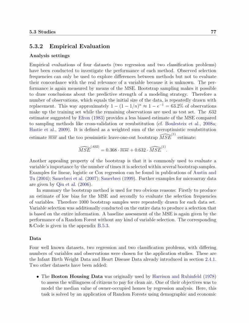
5.3 Studies 77
5.3.2 Empirical Evaluation
Analysis settings
Empirical evaluations of four datasets (two regression and two classification problems)have been conducted to investigate the performance of each method. Observed selectionfrequencies can only be used to explore differences between methods but not to evaluatetheir concordance with the real relevance of a variable because it is unknown. The per-formance is again measured by means of the MSE. Bootstrap sampling makes it possibleto draw conclusions about the predictive strength of a modeling strategy. Therefore anumber of observations, which equals the initial size of the data, is repeatedly drawn withreplacement. This way approximately 1 − (1 − 1/n)n ≈ 1 − e−1 = 63.2% of observationsmake up the training set while the remaining observations are used as test set. The .632estimator suggested by Efron (1983) provides a less biased estimate of the MSE comparedto sampling methods like cross-validation or resubstitution (cf. Boulesteix et al., 2008a;Hastie et al., 2009). It is defined as a weighted sum of the overoptimistic resubstitution
estimate mse and the too pessimistic leave-one-out bootstrap MSE(1)
estimate:
MSE(.632)
= 0.368 ·mse+ 0.632 · MSE(1).
Another appealing property of the bootstrap is that it is commonly used to evaluate avariable’s importance by the number of times it is selected within several bootstrap samples.Examples for linear, logistic or Cox regression can be found in publications of Austin andTu (2004); Sauerbrei et al. (2007); Sauerbrei (1999). Further examples for microarray dataare given by Qiu et al. (2006).
In summary the bootstrap method is used for two obvious reasons: Firstly to producean estimate of low bias for the MSE and secondly to evaluate the selection frequenciesof variables. Therefore 1000 bootstrap samples were repeatedly drawn for each data set.Variable selection was additionally conducted on the entire data to produce a selection thatis based on the entire information. A baseline assessment of the MSE is again given by theperformance of a Random Forest without any kind of variable selection. The correspondingR-Code is given in the appendix B.5.3.
Data
Four well known datasets, two regression and two classification problems, with differingnumbers of variables and observations were chosen for the application studies. These arethe Infant Birth Weight Data and Heart Disease Data already introduced in section 2.4.1.Two other datasets have been added:
• The Boston Housing Data was originally used by Harrison and Rubinfeld (1978)to assess the willingness of citizens to pay for clean air. One of their objectives was tomodel the median value of owner-occupied homes by regression analysis. Here, thistask is solved by an application of Random Forests using demographic and economic

78 5. A new Variable Selection Method
factors (e.g. crime rate, proportion of land over 25,000 sq. ft., proportion of non-retailbusiness acres per town, a Charles River dummy variable, nitric oxides concentration,average number of rooms per dwelling, proportion of owner-occupied units built priorto 1940, weighted distances to five Boston employment centres, index of accessibilityto radial highways, full-value property-tax rate, pupil-teacher ratio, a factor for theproportion of blacks in the town and the fraction of lower status of the population).The data consists of 506 observations and 13 independent variables.
• The Parkinson’s Disease Detection Dataset contains voice recordings of severalhealthy people and people suffering from Parkinson’s disease. Little et al. (2007)originally used it to investigate new feature extraction and speech analysis methodsfor general voice disorders. The distinction of healthy and diseased people creates aclassification problem which is meant to be solved by the aid of several biomedicalvoice measurements. In total there are 22 independent variables measured on 195observations.
A summary of data characteristics is given in table 5.1. Except for the Infant Birth WeightData which was taken from the R package MASS, the data are provided by the open sourceUCI Machine Learning Repository (Frank and Asuncion, 2010).
Data # obs. # var.regression Birthweight 189 9
B. Housing 506 13classification Heart 270 13
Parkinson 195 22
Table 5.1: Characteristics of data used in the application studies.
5.3.3 Implementation
Analyses of this chapter were again performed with the R system for statistical computing(R Development Core Team, 2011, version 2.14.1). The computation of unbiased RandomForests based on a conditional inference framework is provided by the function cforest()
which is part of the package party (Hothorn et al., 2008, version 1.0-0). Each RandomForest contained ntree = 100 trees. The number of randomly selected candidate variablesfor splits ntry was chosen to be the square root of available variables, following the recom-mendation of Dıaz-Uriarte and Alvarez de Andres (2006). Sticking to the default settingmincriterion = 0, there were no restrictions concerning the significance of a split. Treeswere grown until terminal nodes contained less than minsplit = 20 observations while childnodes had to contain at least minbucket = 7 observations.

5.4 Results 79
5.3.4 Settings of Variable Selection Approaches
The variable selection methods presented in section 5.2 were implemented as R-functions(corresponding codes are given in the appendix B.5.1). Although the instructions of authorswere closely followed, a minor adjustment was made for the performance-based approaches.The rejection of a certain fraction of variables was reduced to one variable in each stepin order to investigate a finer grid. Another adaption, which deviates from the originaldefinitions but is felt to be a major improvement, is that performance-based approacheswere empowered to select no variables at all. Therefore the prediction of such a null-modelis simply given by the majority vote of classes (for binary outcomes) or the mean outcome(for continuous outcomes). The resulting MSE is compared to the performance of RandomForests at different variable selection stages. Within the algorithm it technically representsone of the MSE values that can be chosen to be optimal e.g. according to the 1 s.e. rule.
For test-based approaches tests were conducted in a one-sided manner as only valueson the right margin of the empirical distribution of importance measures (i.e. high valuesas opposed to low or negative values) provide evidence against the null-hypothesis of anon-relevant variable.
The performance-based approaches have originally been constructed for classificationproblems only. Consequently, the discussion and presentation of results focus on suchdata. Technically, they are applicable to regression problems, too. However, in such casesonly the 0 s.e. rule is executed to stick close to the original definitions. In principle, andthis is subject to further research, Breiman et al. (1984) already suggested an adaption ofthe 1 s.e. rule for regression analysis. In addition there have been proposals of advancedcross-validation to select optimal models in linear regression analysis (Shao, 1993; Zhang,1993). If adapted to the performance-based variable selection approaches, such methodscould prove beneficial to reduce type-I errors, i.e. lessen the selection of non-relevantvariables. Likewise, the s.e. rule could serve as a kind of tuning parameter for this purpose.Furthermore, the test-based approaches can easily be modified to potentially control forthe TWER and FWER in the same manner as the new proposal.
A summary of all variable selection methods and specific settings is given in Table 5.2.It also contains a list of labels which will be used to name the methods in the following.The algorithms themselves are presented in section 5.2.
5.4 Results
5.4.1 Simulation Studies
Study I
Study I was designed to explore the TWER and FWER of the variable selection approachesfor non-relevant variables. Table 5.3 shows that the approaches NAP, NAP.B and ALT areable to control the TWER of 5%. NAP.B meets the expectations and even controls theFWER due to the application of the Bonferroni-Adjustment. Although other approaches
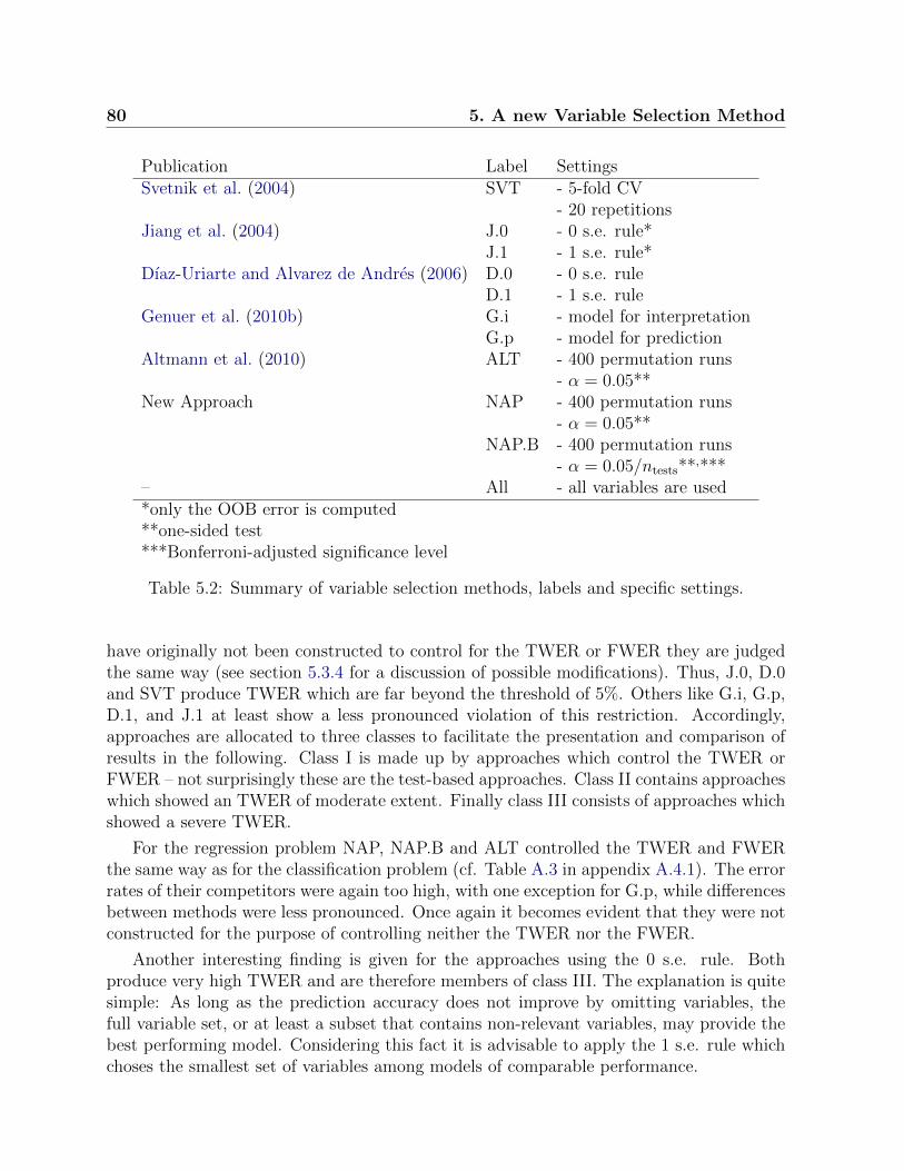
80 5. A new Variable Selection Method
Publication Label SettingsSvetnik et al. (2004) SVT - 5-fold CV
- 20 repetitionsJiang et al. (2004) J.0 - 0 s.e. rule*
J.1 - 1 s.e. rule*Dıaz-Uriarte and Alvarez de Andres (2006) D.0 - 0 s.e. rule
D.1 - 1 s.e. ruleGenuer et al. (2010b) G.i - model for interpretation
G.p - model for predictionAltmann et al. (2010) ALT - 400 permutation runs
- α = 0.05**New Approach NAP - 400 permutation runs
- α = 0.05**NAP.B - 400 permutation runs
- α = 0.05/ntests**,***– All - all variables are used*only the OOB error is computed**one-sided test***Bonferroni-adjusted significance level
Table 5.2: Summary of variable selection methods, labels and specific settings.
have originally not been constructed to control for the TWER or FWER they are judgedthe same way (see section 5.3.4 for a discussion of possible modifications). Thus, J.0, D.0and SVT produce TWER which are far beyond the threshold of 5%. Others like G.i, G.p,D.1, and J.1 at least show a less pronounced violation of this restriction. Accordingly,approaches are allocated to three classes to facilitate the presentation and comparison ofresults in the following. Class I is made up by approaches which control the TWER orFWER – not surprisingly these are the test-based approaches. Class II contains approacheswhich showed an TWER of moderate extent. Finally class III consists of approaches whichshowed a severe TWER.
For the regression problem NAP, NAP.B and ALT controlled the TWER and FWERthe same way as for the classification problem (cf. Table A.3 in appendix A.4.1). The errorrates of their competitors were again too high, with one exception for G.p, while differencesbetween methods were less pronounced. Once again it becomes evident that they were notconstructed for the purpose of controlling neither the TWER nor the FWER.
Another interesting finding is given for the approaches using the 0 s.e. rule. Bothproduce very high TWER and are therefore members of class III. The explanation is quitesimple: As long as the prediction accuracy does not improve by omitting variables, thefull variable set, or at least a subset that contains non-relevant variables, may provide thebest performing model. Considering this fact it is advisable to apply the 1 s.e. rule whichchoses the smallest set of variables among models of comparable performance.

5.4 Results 81
TWER FWER Classvar. 1 var. 2 var. 3 var. 4 var. 5
NAP.B 1.0% 0.8% 0.7% 1.2% 0.9% 4.4% INAP 5.1% 5.0% 4.9% 5.7% 5.3% 22.7% IALT 5.3% 4.7% 5.0% 5.2% 5.2% 23.3% IG.p 9.2% 9.1% 8.6% 9.9% 9.4% 40.6% IID.1 13.9% 14.8% 14.4% 15.1% 14.9% 49.7% IIJ.1 14.1% 14.8% 14.8% 15.2% 15.1% 54.0% IIG.i 18.7% 19.1% 18.4% 20.0% 19.7% 64.2% IIJ.0 29.1% 28.5% 28.7% 29.8% 29.9% 79.7% IIID.0 29.1% 29.3% 29.7% 29.5% 30.6% 75.7% IIISVT 29.7% 29.6% 29.1% 29.8% 30.2% 58.9% III
Table 5.3: TWER and FWER for 5000 simulation runs of the classification problem instudy I. Approaches are ranked and allocated to classes I, II and III according to theirmean TWER.
Study II
Study II was designed to investigate the power of the approaches to discriminate relevantfrom non-relevant variables. Results are shown by Figure 5.2 which displays the observedselection frequencies against a rising strength s of the predictor variables. For a clearpresentation, classes are subsumed by gray areas which range from the lowest to highestvalues observed for the corresponding approaches. The evident discrepancy of classesconfirms the definition found in study I. A more detailed view and discussion of eachapproach is given in the appendix A.4.1.
An examination of selection frequencies for the non-relevant variable 6, and variables1, 3, and 5 when s = 0, makes it clear that approaches of class III heavily exceed theTWER of 5% (which is indicated by a horizontal line in the plots). Accordingly, it is notsurprising that they also show a high power to detect the relevant variables 1, 2, 3, 4 and5 (when s > 0). However, this comes at the cost of a high TWER. It is also interestingto note that for some of the approaches, the selection frequency of the relevant variable 4even drops with a rising strength of variables 1, 2 and 3. The new approaches NAP andNAP.B show competitive and in some cases even superior results though they control theTWER, or even the FWER in the case of NAP.B.
Results for class II (+ ALT) indicate that these approaches are much more capableto control the TWER. However, in the majority of cases they are outperformed by NAPand NAP.B which show a much higher power to select the relevant variables. The newapproaches also seem to be the only ones which are able to detect variable 5, which is non-informative yet relevant as it is correlated to the informative variable 3. They also showa constant selection frequency for variable 4 – independent of the amount and strength ofinformative variables.

82 5. A new Variable Selection Method
0
200
400
600
800
1000
variable 1
NAPNAP.B
upper: class IIIlower: class II (+ ALT)
variable 2
0
200
400
600
800
1000
sele
ctio
n fr
eque
ncy
variable 3 variable 4
0
200
400
600
800
1000
0 0.1 0.2 0.3 0.4 0.5 0.6 0.7 0.8 0.9 1s =
variable 5
0 0.1 0.2 0.3 0.4 0.5 0.6 0.7 0.8 0.9 1
variable 6
Figure 5.2: Plot of selection frequencies in 1000 simulation runs of the classification problemof study II. Results are shown in dependence of predictor strength as determined by βII =(s, s, s, 1, 0, 0)>. There are no relations except for pairwise correlations (r = 0.7) betweenvariable 2 and 4 as well as 3 and 5. Class III and II (+ ALT) are represented by gray areaswhich range from the lowest to highest values observed for the corresponding approaches.The horizontal line represents a 5% TWER. [Relevant Variables: var. 4 & var. 1, 2, 3, 5for s > 0; Informative Variables: var. 4 & var. 1, 2, 3 for s > 0]

5.4 Results 83
Results for the regression problem show a clear superiority of the new approacheswhich is even more demonstrative than in the classification problem (cf. Figure A.7 in theappendix A.4.1). NAP and NAP.B once again outperform their competitors in terms ofdiscriminatory power.
Study III
Figure 5.3 displays results for variables 1–15 of study III (the non-relevant variables 16–20were omitted from the illustration for redundancy). The presentation is again grouped byclass and a more detailed discussion of each approach is given in appendix A.4.1. As ageneral finding, it is interesting to note that variables of correlated blocks (var. 4–11) showhigher selection frequencies than uncorrelated variables (var. 1–3), even though the formermight be non-informative (var. 10–11). This is due to the sensitivity of unconditionalimportance measures to relations between variables (cf. Strobl et al., 2008).
An investigation of selection frequencies for variables 12-15 makes clear that approachesof class III again select non-relevant variables far too often – confirming the results of studiesI and II. Despite this increased TWER they are not able to outperform NAP and in mostcases even the opposite is true when it comes to the identification of the relevant variables1–11. Even NAP.B, which by definition is much more conservative, is able to keep up withthese approaches in some cases. All methods of class II (+ ALT) produce a TWER ofabout 5% and therefore also agree with the findings of Study II. A comparison reveals aclear superiority of NAP and NAP.B in terms of the ability to identify relevant variables.
It is also interesting to note that a precise interpretation of equation (5.1) suggeststhat even a relation between non-informative variables could theoretically provide evidenceagainst H0. However, this is not a grave issue as in practice the computation of importancemeasures underlying the hypothesis tests is only affected by relations of variables to theresponse, whether they are direct or achieved via correlation. Therefore, NAP and NAP.Bdid not select the correlated and non-informative variables 12 and 13. This is a desirableproperty as it perfectly matches the definition of non-relevance (cf. section 5.1) whichdemands that a relevant variable is either informative itself or correlated to an informativeone.
Once again, results demonstrate that the new approaches show a high power to distin-guish relevant from non-relevant variables among approaches which either tend to selectany kind of variable (class III), not matter their relevance, or are too weak to detect relevantvariables (class II).
Boxplots of the observed MSE values show that among all variable selection approaches,NAP performs best while NAP.B is in the sixth position. However, it has to be pointedout that all results up to and including NAP.B are on a comparable level. Results alsounderline the well known fact that the prediction accuracy of Random Forests does notnecessarily benefit from variable selection: the Random Forest which was build withoutany selection performs best.
In a perfect scenario all of the selected variables are relevant while the non-relevantones are rejected. An additional illustration of mean selection frequencies investigates this

84 5. A new Variable Selection Method
property. The second best performing approach SVT selected 10.7 variables on average.Among those, 9 variables were of relevance. This makes a difference of 1.7 (16%) selectedbut non-relevant variables. Results for D.0 and J.0 are even worse. NAP only selects 9.2variables but as much as 8.8 relevant ones. This makes a difference of 0.4 (4%) while theabsolute amount of selected relevant variables is almost as high as for SVT (8.8 vs. 9).Thus for the selection of an equal number of relevant variables NAP produces less falsepositive detections. These values are even lower for NAP.B and ALT (0.1 and 0; 2% and0%), although the absolute amount of detected relevant variables is lower (6.5 and 6.7).In conclusion NAP and NAP.B show a high efficiency as the fraction of relevant variablesamong a set of selected variables is high. NAP is also more effective as the absoluteamount of detected relevant variables is high, too. Meanwhile they are able to produce acomparable MSE while other approaches are less efficient and less effective.
In the regression problem the new approaches NAP and NAP.B outperform their com-petitors even more clearly (see Figure A.9 in appendix A.4.1). They show the highestpower to detect relevant variables, produce the lowest median MSE (even lower than fora Random Forest without any variable selection) and show effectivenesses and efficienciesthat range among the highest.
5.4.2 Empirical Evaluation
A summary of results found for the empirical evaluation is given by Table 5.4. It revealsthat the new variable selection approaches, compared to eight competitors, are consistentlyranked among the best performing ones. In some instances they are even able to beat theperformance of a Random Forest that uses no variable selection. It is also remarkable thatmethods of class II and III show alternating performance rankings while they can clearlybe differentiated from class I which achieves better results throughout.
The number of selected variables for each classification and regression problem differsbetween methods. A comparison of performances makes clear that an increased or de-creased set of variables is not necessarily associated with prediction accuracy. Likewise,it is not possible to rate the quality or correctness of selections as the true relevance ofvariables is unknown for real data (section 5.4.1 for similar evaluations). However, thenumber of times a variable is selected across all bootstrap runs may at least be taken asan indicator for its importance and the stability of its selection (cf. Table A.4 in appendixA.4.2). Considering the achieved performances, NAP and NAP.B seem to be well suitedto select variables which are of predictive relevance.
5.5 Discussion and Conclusion
An extensive review of literature about variable selection using Random Forests led tothe proposal of a new approach. It was basically invented within a permutation testframework to meet important theoretical properties. In addition, three simulation studiesshowed further appealing properties: Firstly, the new approach makes it possible to control

5.5 Discussion and Conclusion 85
sele
lctio
n fr
eque
ncy
0
200
400
600
800
1000
3 2 1 (3 2 1) (3 2 1 0 0) (0 0) 0 01 2 3 4 5 6 7 8 9 10 11 12 13 14 15variable =
coefficient =
(a)
NAPNAP.B
upper: class IIIlower: class II (+ ALT)
●●
●
●
●●●
●
●
●●●●
●
●●●● ●
●●
●
●
●
●
●
●●
●
●
●●●●
●●
●
●●●●
●
●
●
●
●
●
●●
●
●
●●
●
●
●●
●
●
●
●
●●
●●
●
●
●
●
●
●
●
●
●
●●
●
●●
●
●●●●●
●●●●
●
●
●
●
●
●
●
●
●
●
●
●
●●
●
●
●●
●
●
●
●
●
●
●●
●
●●
●●●
●●●●
●●
●●●
●
●
●
●
●●
●
●
●●
●●
●
●
●
●●
●
●●●●●●
●●●●●●
●●
●●●●●
●●●●●●
●
●●●●
●
●
●●●●●●
●
●●
●
●●
●●
●●
●
●●
●
●●●●
●
●●
●●●●
●
●
●
●●
●●
●
●
All NAP SVT D.0 ALT J.0 NAP.B G.i D.1 J.1 G.p
0.10
0.15
0.20
0.25
0.30
0.35
0.40
0.45
MS
E
(b)
0.188 0.192 0.194 0.201 0.202 0.202 0.204 0.215 0.218 0.221 0.251med. =
All NAP SVT D.0 ALT J.0 NAP.B G.i D.1 J.1 G.p
mea
n se
lect
ion
freq
uenc
y
0
5
10
15
20
(c)
20
9.210.7 10.7
6.7
10.1
6.54.7 5 4.3
2.4
11
8.8 98.2
6.77.7
6.44.7 4.7 4.2
2.4
9
7 7.3 6.85.6
6.45.4
4.3 4.2 3.82.2
var. selected # relevant # informative
Figure 5.3: (a) Selection frequencies of variables 1–15 in 1000 simulation runs of the clas-sification problem of study III. Class III and II (+ ALT) are represented by gray areaswhich range from the lowest to highest values observed for the corresponding approaches.The horizontal line represents a 5% TWER. Brackets indicate correlated variables. (b)Boxplots of the observed MSE aranged in increasing order of median values. (c) Mean se-lection frequency of variables and an additional information about the amount of relevantand informative variables among them. Reference values are indicated by horizontal lines.[Relevant Variables: var. 1 – 11; Informative Variables: var. 1 – 9]

86 5. A new Variable Selection Method
Rank 1 2 3 4 5 6 7 8 9 10 11
Birthweight NAP.B NAP ALT G.p G.i SVT All D.0 J.0class I I I II II III III III
MSE(1)
0.208 0.213 0.209 0.209 0.209 0.210 0.227 0.315 0.309var. selected 5.80 7.25 4.99 1.00 1.22 1.09 9.00 5.18 5.01
mse 0.166 0.169 0.192 0.203 0.203 0.203 0.191 0.272 0.319var. selected 5 5 3 1 1 1 9 5 5
MSE(.632)
0.193 0.197 0.203 0.207 0.207 0.207 0.214 0.299 0.312
B. Housing ALT NAP.B NAP All SVT G.i G.p D.0 J.0class I I I III II II III III
MSE(1)
16.31 16.61 16.70 16.79 20.22 20.05 20.10 27.30 26.71var. selected 9.39 12.56 12.83 13.00 2.78 2.63 2.09 9.01 8.81
mse 10.78 10.33 10.91 11.63 11.86 14.94 14.95 15.79 18.15var. selected 7 13 13 13 3 2 2 7 10
MSE(.632)
14.27 14.30 14.57 14.89 17.14 18.17 18.20 23.07 23.56
Heart All NAP NAP.B ALT SVT D.0 G.i J.1 D.1 J.0 G.pclass I I I III III II II II III II
MSE(1)
0.173 0.175 0.177 0.180 0.175 0.177 0.181 0.181 0.182 0.177 0.248var. selected 13.00 11.44 9.94 7.54 10.42 9.79 5.19 5.78 5.99 9.53 1.99
mse 0.100 0.118 0.122 0.126 0.137 0.137 0.137 0.137 0.137 0.170 0.237var. selected 13 10 8 7 11 3 3 3 3 4 1
MSE(.632)
0.146 0.154 0.157 0.160 0.161 0.162 0.165 0.165 0.165 0.174 0.244
Parkinson NAP All NAP.B ALT J.0 D.0 SVT J.1 G.i D.1 G.pclass I I I III III III II II II II
MSE(1)
0.152 0.153 0.152 0.152 0.150 0.151 0.155 0.152 0.153 0.155 0.162var. selected 19.16 22.00 13.54 9.83 11.27 12.74 11.26 4.92 5.53 5.77 1.94
mse 0.092 0.097 0.103 0.108 0.113 0.113 0.108 0.133 0.133 0.133 0.133var. selected 14 22 10 5 19 14 14 1 1 1 1
MSE(.632)
0.130 0.133 0.134 0.136 0.136 0.137 0.138 0.145 0.146 0.147 0.152
Table 5.4: Bootstrap-, resubstitution- and .632 estimators for the MSE of the investigated
methods arranged in order of decreasing performance (assessed by MSE(.632)
) for eachdatasset. In addition, the average number of selected variables in the bootstrap runs andfor a single fit on the entire dataset are given.
the TWER and FWER. Secondly, it showed a higher power to distinguish relevant fromnon-relevant variables compared to common approaches. This finding was also confirmedin a simulated data application. Thirdly, it achieved the highest ratio of relevant to selectedvariables. Corresponding Random Forests produced MSE values which were comparable tothe best performing models. Within an application to four datasets the two versions of thenew approach always ranked among the best three (out of eleven) performing approaches interms of MSE. Moreover, it is equally applicable to regression and classification problems.
Despite the clear superiority of the new approach which was observed in this work, thebenefit of its application, in terms of prediction accuracy and especially for the selectionof relevant variables, has to be further investigated. Additional simulation studies andempirical evaluations, possibly emerging from research fields in which these approachesare commonly used (e.g. microarray analysis, GWAS), are needed for further insight.Investigations should be intensified to further explore the effects of correlation strength,block size, interactions, type of importance measure, definition of ‘relevance’ and kind ofalpha adjustment. Analyses also need to be extended to high-dimensional data.

Chapter 6
Variable Selection with Missing Data
6.1 Research Motivation and Contribution
Variable selection has been suggested for Random Forests to enhance data prediction andinterpretation (cf. chapter 5). However, its basic element, i.e. variable importance mea-sures, can not be computed in a straightforward manner when there are missing data(chapter 3). Possible solutions that still enable variable selection despite the occurrence ofmissing values are
• complete case analysis,
• multiple imputation and
• the new importance measure.
These have been used in combination with two variable selection methods:
• NAP and
• D.1,
representing the conceptual classes of test-based and performance-based approaches, re-spectively (section 5.3.4). An extensive simulation study that involves various missing datagenerating processes is conducted to explore their ability to discriminate relevant from non-relevant variables. In addition, the predictive accuracy of resulting models is investigatedfor a simulated test dataset (see chapter 2 and 4 for similar studies). Both regression andclassification problems are explored. Findings and recommendations: Complete case anal-ysis should not be applied as it leads to inaccurate variable selection and models with theworst prediction accuracy. Multiple imputation is a good means to select variables thatwould be of relevance in fully observed data. It produced the best prediction accuracy.By contrast, the application of the new importance measure causes a selection of variablesthat reflects the actual data situation, i.e. that takes the occurrence of missing values intoaccount. Its error was only negligibly worse compared to imputation.

88 6. Variable Selection with Missing Data
6.2 Simulation Studies
An extensive simulation study was set up to explore which of complete case analysis, mul-tiple imputation by MICE and the new importance measure is most capable of supportingvariable selection. Therefore the NAP and D.1 approaches, as representatives of test-basedand performance-based methods, have been chosen to investigate their quality to distin-guish relevant from non-relevant variables. Two additional investigations will focus on thepredictive accuracy of Random Forests in a simulated test dataset and the ability of selec-tion methods to control the TWER. Factors like the amount of missing values, correlationschemes, variable strength and different missing data generating processes are of majorinterest as they potentially influence variable selection. The setup of the simulation studyresembles the ones given in chapter 3 and 4. Essential differences are presented in thefollowing:
• Influence of predictor variables
The simulated data contained both a classification and a regression problem. There-fore, a categorical (binary) and a continuous response were created in dependence ofsix variables with coefficients β:
β = (1, 1, 0, 1, 1, 0)>.
Repeated values for β make it possible to compare selection frequencies of variableswhich are, by construction, equally important but show different correlations andcontain different amounts of missing values. In addition, the non-influential variableswith β = 0 help to investigate possible undesired effects, serve as a baseline and areused to check for the ability to control the TWER.
• Correlation
Σ =
1 0.3 0.3 0 0 0
0.3 1 0.3 0 0 00.3 0.3 1 0 0 0
0 0 0 1 0 00 0 0 0 1 00 0 0 0 0 1
As the variances of each variable are chosen to be 1, the covariance equals the cor-relation in this special case. The structure of the covariance matrix Σ reveals thatthere are two blocks of three correlated and three uncorrelated variables.
• Missing values
Several missing data generating processes that follow MCAR, MAR and MNARschemes were employed. For each, a given fraction m ∈ {0.0, 0.1, 0.2, 0.3} of values isset missing in variables X2 and X5 (cf. Table 6.1). Therefore, the average percentageof observations that contain at least one missing value is 1− (1−%missing)nvariables =

6.3 Results 89
contains missing values determines missing values(MCAR, MAR & MNAR) (MAR) (MNAR)X2 X1 X2
X5 X4 X5
Table 6.1: List of variables that contain missing values and determine the probability ofmissing values.
1−(1−0.3)2 = 51% in case of m = 0.3. This is an amount not unlikely to be observedin real life data which makes m span a wide range of possible scenarios. The schemesto produce missing values were MCAR, MAR(rank), MAR(median), MAR(upper),MAR(margins) and MNAR(upper).
• Validation
An independent test dataset of 5000 observations was constructed the same way,though it did not contain missing values, for an evaluation of predictive accuracy.The latter was assessed by the mean squared error (MSE) which equals the misclas-sification error rate (MER) in classification problems.
• Implementation
The implementation of the simulation almost equals the one of chapter 4 except forthe fact that Random Forests contained more trees: ntree = 100. CorrespondingR-Code is given in section B.6.
In summary, there were 2 variable selection methods and 2 response types investigated for6 processes to generate and 3 procedures to handle 4 different fractions of missing values.This sums up to 288 simulation settings. Each of them was repeated 1000 times.
6.3 Results
The following discussion presents results for the classification problem. Similar findingsfor the regression problem are given as supplementary material in section A.5 (cf. FigureA.10)
Variable selection frequencies displayed in Figure 6.1 stress that the test-based ap-proach performs better than the performance-based approach. The former selects relevantvariables (including variable 3 which is non-informative, yet correlated to informative vari-ables) more often, independent of the amount of missing values. With reference to thenon-relevant variable 6, both approaches control for the TWER. As expected, the selectionfrequencies of variables 2 and 5 drop as they contain a rising amount of missing values.Meanwhile variables 1 and 4 are chosen more frequently by the performance-based ap-proach. This can be seen as the attempt to replace variables with missing information byother predictors (see chapter 3). The same effect can not be observed for the test-based

90 6. Variable Selection with Missing Data
● ● ● ● ● ● ● ●
● ● ● ●
● ● ● ● ●●
●●
● ● ● ●0200400600800
1000
.0 .1 .2 .3 .0 .1 .2 .3 .0 .1 .2 .3 .0 .1 .2 .3 .0 .1 .2 .3 .0 .1 .2 .3m =
MC
AR
● test−based ( performance−based (● contains missings) contains missings)
● ● ● ● ● ● ● ●
● ● ● ●
● ● ● ● ●●
● ●
● ● ● ●0200400600800
1000
MA
R(r
ank)
● ● ● ● ● ● ● ●
● ● ● ●
● ● ● ● ● ●● ●
● ● ● ●0200400600800
1000
MA
R(m
edia
n)
● ● ● ● ● ● ● ●
● ● ● ●
● ● ● ● ● ● ● ●
● ● ● ●0200400600800
1000
MA
R(u
pper
)
● ● ● ● ● ● ●●
● ● ● ●
● ● ● ● ● ● ● ●
● ● ● ●0200400600800
1000
MA
R(m
argi
ns)
● ● ● ● ●●
●●
● ● ● ●
● ● ● ● ●
●●
●
● ● ● ●0200400600800
1000
1 2 3 4 5 6variable
MN
AR
(upp
er)
sele
ctio
n fr
eque
ncy
Figure 6.1: Variable selection frequencies observed for the new importance measure. Thehorizontal dashed line illustrates a TWER of 5% (m = % of missing values in X2 and X5).
approach which already shows higher and rather stable selection frequencies for these fullyobserved variables. There are minor differences between variables 1 and 4, though they areof the same strength. This is due to the fact that unconditional permutation importancemeasures, which underly the applied selection methods, rate the relevance of correlatedvariables higher than for uncorrelated ones (Strobl et al., 2008). In conclusion, there areno apparent differences between the missing data generating processes. The applicationof the new importance measure for variable selection can be recommended whenever theobjective is to describe the data situation at hand; i.e. under consideration of the relevancea variable can take with all of its missing values.
In the complete case analysis (illustrated by Figure 6.2) the performance-based ap-proach is again outperformed by the test-based approach, while both control for the TWER.However, there are some general findings that question the quality of complete case anal-ysis. Thus, selection frequencies of the informative variables 1 and 4 drop with a risingfraction of missing values in variables 2 and 5. One might argue that this is caused bythe general loss of information induced by complete case analysis. However, in some cases(e.g. MAR(margins)) this effect is carried to extremes as variables 1 and 4 are even lessfrequently selected than variables 2 and 5, while the latter are the ones that actually lostpart of their information. There is no rational justification for this undesirable propertywhich is present for any missing data generating process. Consequently, complete caseanalysis is not recommended for application as selection methods might not be capable ofdetecting variables of true relevance.

6.3 Results 91
● ●●
●
● ●●
●
● ● ● ●
●●
●●
●●
●●
● ● ● ●0200400600800
1000
.0 .1 .2 .3 .0 .1 .2 .3 .0 .1 .2 .3 .0 .1 .2 .3 .0 .1 .2 .3 .0 .1 .2 .3m =
MC
AR
● test−based ( performance−based (● contains missings) contains missings)
● ●●
●
● ●●
●
● ● ● ●
●●
●●
●●
●●
● ● ● ●0200400600800
1000
MA
R(r
ank)
● ●●
●
● ●●
●
● ● ● ●
●●
●●
●●
●●
● ● ● ●0200400600800
1000
MA
R(m
edia
n)
●
●
●
●
●●
●
●
● ● ● ●
●
●
●
●
● ●●
●
● ● ● ●0200400600800
1000
MA
R(u
pper
)
●
●
●
●
●●
●●
● ● ● ●
●
●
●●
● ● ●●
● ● ● ●0200400600800
1000
MA
R(m
argi
ns)
● ●●
●
●
●
●
●● ● ● ●
● ●●
●
●
●
●
●
● ● ● ●0200400600800
1000
1 2 3 4 5 6variable
MN
AR
(upp
er)
sele
ctio
n fr
eque
ncy
Figure 6.2: Variable selection frequencies observed for the complete case analysis. Thehorizontal dashed line illustrates a TWER of 5% (m = % of missing values in X2 and X5).
Results for the application of multiple imputation are given by Figure 6.3. Again, theyreflect the superiority of the test-based approach to the performance-based approach, whileboth of them control the TWER. Furthermore, imputation leads to rather stable selectionfrequencies of variables, independent of the amount of missing values. However, a slightdecrease can still be observed for variables 2 and 5 as they lose information. This holds foreach missing data generating process except for MNAR(upper). It is interesting to notethat results for the latter resemble those of Figure 6.1. Thus, the occurrence of missingvalues and the associated loss of information seems to directly affect selection frequencieswhen missing values can not be appropriately imputed. Nevertheless, multiple imputationappears to be a well suited means of selecting variables according to the relevance theywould have if the data were fully observed.
Prediction errors observed for the independent test sample are displayed by Figure 6.4.They confirm the superiority of the test-based approach to the performance-based approachin terms of predictive accuracy. This holds independent of the approach to handle missingvalues, the amount of missing values and the process to generate missing values. The lowestMSE, which is almost stable for any fraction of missing values, was found for models fit toimputed data. Variable selection that is based on the new importance measure producedmodels that performed only slightly worse (see chapter 2 and 4 for corresponding findings).For this procedure the error increased with an increasing number of missing values. Thisproperty intensifies for the complete case analysis which clearly produced the worst resultsfor increased fractions of missing values. Similar findings about the predictive accuracy of
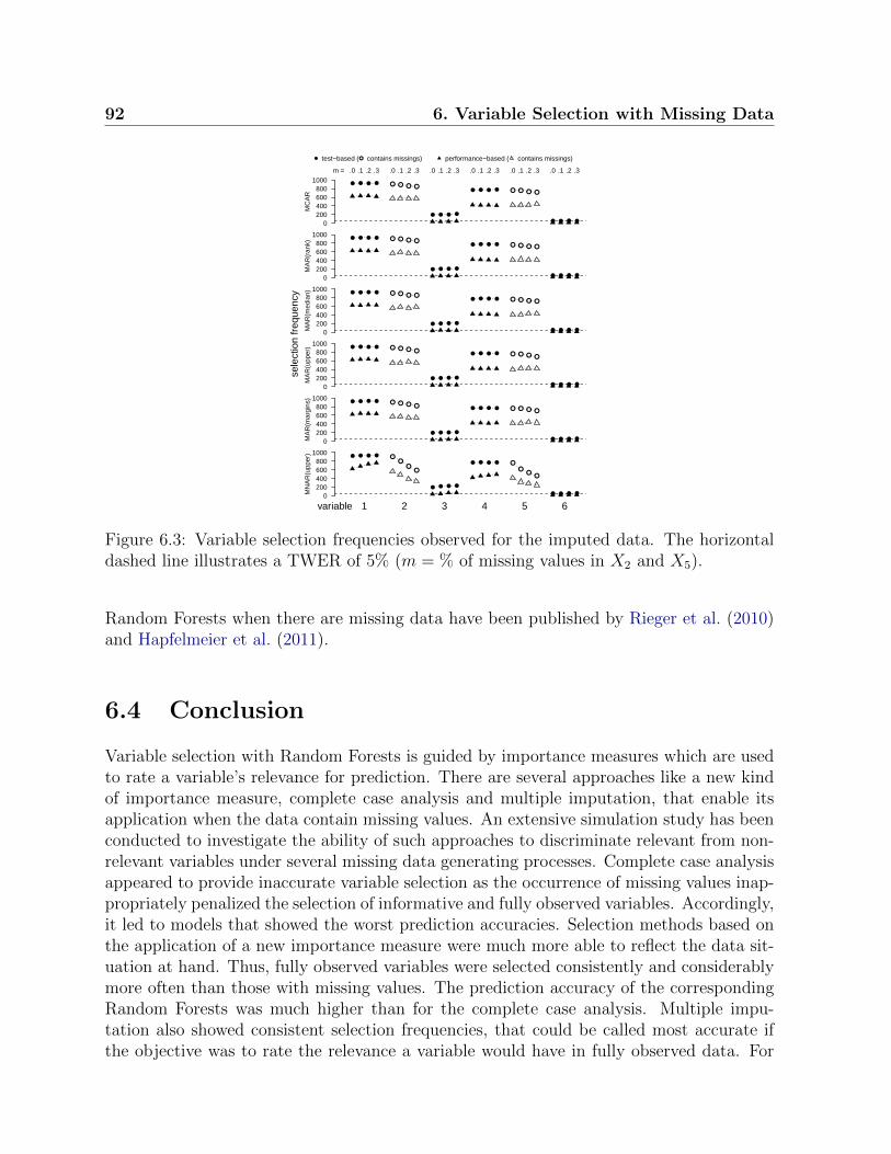
92 6. Variable Selection with Missing Data
● ● ● ● ● ● ● ●
● ● ● ●
● ● ● ● ● ● ● ●
● ● ● ●0200400600800
1000
.0 .1 .2 .3 .0 .1 .2 .3 .0 .1 .2 .3 .0 .1 .2 .3 .0 .1 .2 .3 .0 .1 .2 .3m =
MC
AR
● test−based ( performance−based (● contains missings) contains missings)
● ● ● ● ● ● ● ●
● ● ● ●
● ● ● ● ● ● ● ●
● ● ● ●0200400600800
1000
MA
R(r
ank)
● ● ● ● ● ● ● ●
● ● ● ●
● ● ● ● ● ● ● ●
● ● ● ●0200400600800
1000
MA
R(m
edia
n)
● ● ● ● ● ● ● ●
● ● ● ●
● ● ● ● ● ● ● ●
● ● ● ●0200400600800
1000
MA
R(u
pper
)
● ● ● ● ● ● ● ●
● ● ● ●
● ● ● ● ● ● ● ●
● ● ● ●0200400600800
1000
MA
R(m
argi
ns)
● ● ● ● ●●
●●
● ● ● ●
● ● ● ● ●●
●●
● ● ● ●0200400600800
1000
1 2 3 4 5 6variable
MN
AR
(upp
er)
sele
ctio
n fr
eque
ncy
Figure 6.3: Variable selection frequencies observed for the imputed data. The horizontaldashed line illustrates a TWER of 5% (m = % of missing values in X2 and X5).
Random Forests when there are missing data have been published by Rieger et al. (2010)and Hapfelmeier et al. (2011).
6.4 Conclusion
Variable selection with Random Forests is guided by importance measures which are usedto rate a variable’s relevance for prediction. There are several approaches like a new kindof importance measure, complete case analysis and multiple imputation, that enable itsapplication when the data contain missing values. An extensive simulation study has beenconducted to investigate the ability of such approaches to discriminate relevant from non-relevant variables under several missing data generating processes. Complete case analysisappeared to provide inaccurate variable selection as the occurrence of missing values inap-propriately penalized the selection of informative and fully observed variables. Accordingly,it led to models that showed the worst prediction accuracies. Selection methods based onthe application of a new importance measure were much more able to reflect the data sit-uation at hand. Thus, fully observed variables were selected consistently and considerablymore often than those with missing values. The prediction accuracy of the correspondingRandom Forests was much higher than for the complete case analysis. Multiple impu-tation also showed consistent selection frequencies, that could be called most accurate ifthe objective was to rate the relevance a variable would have in fully observed data. For

6.4 Conclusion 93
0.200.250.300.350.400.45
MCAR
new measure imputation complete case
test−based performance−based
0.200.250.300.350.400.45
MAR(rank)
0.200.250.300.350.400.45
MAR(median)
0.200.250.300.350.400.45
MAR(upper)
0.200.250.300.350.400.45
MAR(margins)
0.200.250.300.350.400.45
MNAR(upper)
.0 .1 .2 .3 .0 .1 .2 .3 .0 .1 .2 .3m =
MS
E
Figure 6.4: MSE observed for the independent test sample. Outliers are not displayed forclarity (m = % of missing values in X2 and X5).
any simulation setting and any approach to handle missing values, the test-based variableselection method performed better than the performance-based approach.
There is a clear recommendation for the application of approaches: One should not usecomplete case analysis because of inaccurate selection properties. Approaches that baseon the new kind of importance measure should be used if one is interested in a selectionof variables that reflects their relevance under consideration of the given information. Bycontrast, imputation methods are best used for the selection of variables that would be ofrelevance in the hypothetical scenario of fully observed data.

94 Outlook

Outlook
The assessment of predictive accuracy has been performed for the newly introduced variableimportance, complete case analysis and multiple imputation in chapter 2, 4 and 6. However,investigations need to be expanded:
• A concluding discussion in section 2.3.2 already presents some recent and ongoingdevelopments of imputation methods. This diversity of approaches should be takeninto account for future research.
• Despite elaborate simulation settings and extensive empirical evaluations the findingsneed to prove generalisability in further investigations.
A new variable importance measure for Random Forests with missing data is proposedin chapter 3. Although it meets all postulated requirements and shows some appealingcharacteristics the corresponding discussions have shown that there is still room for furtherdevelopments and investigations:
• A conditional variable importance measure that can handle missing data is to bedeveloped. Strobl et al. (2008) introduced a conditional version of the permutationaccuracy importance measure that more closely resembles the behavior of partialcorrelation or regression coefficients. Yet, non-conditional importance measures, towhich the one proposed in chapter 3 belongs to, are often appreciated for theirsensitivity to correlations and hence for their ability to uncover relations betweenvariables (see chapter 5 for further discussions of this matter). However, in someresearch fields a conditional assessment might be preferred which raises the task ofenhancing the current method to a measure that, besides its property to handlemissing values, is conditional.
Chapter 5 presents an extensive investigation of a new variable selection procedure forRandom Forests. Despite its appealing properties and power to distinguish relevant fromnon-relevant variables, future research and further developments are proposed to enhanceits applicability:
• As the permutation steps of the proposed test-based variable selection algorithm areindependent from each other they can be parallelized on multiple cores of a systemto significantly reduce computation time (see Altmann et al., 2010, for an earliersuggestion of this procedure). In future work this benefit can be checked for andrealized by an according implementation.

96 Outlook
• In section 5.3.4 it has been pointed out that the performance-based approaches haveoriginally been suggested for classification problems only. Thus, corresponding defi-nitions of the 1 s.e. rule are not applicable to regression problems. However, Breimanet al. (1984) already suggested an adaption of the 1 s.e. rule which will be imple-mented for further performance evaluations in regression analysis.
• The application of variable selection with Random Forests is particularly popular inthe field of microarray data analysis (Dıaz-Uriarte and Alvarez de Andres, 2006; Jianget al., 2004; Rodenburg et al., 2008; Zhou et al., 2010). Many of the presented meth-ods were originally designed for this special data case which is characterized by a lowratio of observations to predictors. Accordingly, the properties and competitivenessof the new approach should be reassessed in this special research field.
• There are several aspects like correlation strength, block size, interactions, type of im-portance measure, definition of ‘relevance’ and kind of alpha adjustment that shouldbe the object of further, intensified investigations as to examine their effect on theperformance of variable selection approaches.
• Despite a possible parallelization of the new algorithm, the computation time is ex-pected to be exceptionally high in the case of thousands or tens of thousands ofpredictors. For the analysis of microarray data, this is a well known problem facedby many methods. It becomes even more challenging as more and more geneticinformation is made available with ongoing research, e.g. in GWAS. A proposed so-lution is to reduce the information transfered to the new approach by a preliminaryselection step. Therefore a suggestion of Strobl et al. (2009) is followed: all variableswith an importance which lies within the random variability of non-relevant variables(determined by the range of negative importance measures) are rejected. This waythe amount of variables passed to the new approach is supposed to be significantlyreduced. Especially in the case of microarray data, which can contain lots of redun-dant information, the computational time is expected to decrease substantially dueto this very fast and easy preliminary selection step. Corresponding experience hasalready been published in Yahya et al. (2011).
• The new variable selection approaches proposed in this work are based on an un-conditional importance measure (Strobl et al., 2008, for a definition of conditionaland unconditional measures). For this reason non-informative variables which arerelated to informative ones are found to be of relevance and possibly selected by theapproaches. However, this might also be seen as an undesired property. Future re-search is meant to explore variable selection that is based on a conditional importancemeasure. In this manner, the question of whether the selection can be restricted toinformative variables is meant to be answered, too.

Appendix A
Supplementary Material
A.1 Chapter 2
A.1.1 Simulation Studies
Table A.1 contains an extensive listing of results for the simulation studies presented insection 2.5.
Table A.1: Summary of mean MSE values, mean absolute (abs. imp. = MSESur. −MSEMICE) and mean relative improvement (rel. imp. = MSESur.−MSEMICE
MSESur.) obtained by using
multiple imputation and surrogates. Missing values were induced completely at randominto data that was originally fully observed. Two imputation schemes are distinguished.For one of them all variables and for another one only one third of variables is partlyset missing. Please note that the mean relative improvement is given by the mean ofimprovements across simulation runs. It can not simply be computed by using the meanMSE values in the formula given here (as the mean of ratios does not equal the ratio ofmeans).
missing Surrogates MICE abs. imp. rel. imp.Data Type # Var. % Values Mean SD Mean SD Mean SD Mean SD
Classi- H. Survival forest 0% 0.27 0.05 0.27 0.05fication 3 10% 0.28 0.05 0.27 0.05 0.01 0.03 0.03 0.12
20% 0.29 0.05 0.27 0.05 0.02 0.04 0.05 0.1430% 0.28 0.05 0.27 0.06 0.01 0.04 0.04 0.1540% 0.28 0.06 0.27 0.05 0.00 0.05 0.00 0.18
1 10% 0.27 0.05 0.27 0.05 0.00 0.02 0.00 0.0820% 0.27 0.05 0.27 0.05 0.00 0.03 0.00 0.1030% 0.27 0.05 0.27 0.05 0.00 0.03 0.00 0.1140% 0.27 0.05 0.27 0.05 0.00 0.03 0.00 0.12
ctree 0% 0.28 0.05 0.28 0.053 10% 0.28 0.06 0.28 0.05 0.00 0.04 -0.01 0.18
20% 0.27 0.06 0.27 0.05 0.00 0.05 -0.02 0.1830% 0.27 0.06 0.27 0.06 0.00 0.05 -0.01 0.1640% 0.27 0.06 0.27 0.05 0.00 0.05 -0.02 0.19
1 10% 0.28 0.05 0.28 0.05 0.00 0.03 -0.01 0.1020% 0.28 0.05 0.28 0.05 0.00 0.03 -0.01 0.1030% 0.27 0.05 0.28 0.05 0.00 0.03 -0.02 0.1140% 0.28 0.05 0.28 0.05 0.00 0.03 -0.01 0.11
rpart 0% 0.28 0.05 0.28 0.053 10% 0.28 0.06 0.28 0.05 0.00 0.04 0.00 0.15
20% 0.28 0.05 0.28 0.05 0.00 0.04 -0.01 0.1630% 0.28 0.05 0.28 0.06 0.00 0.04 -0.01 0.1740% 0.28 0.05 0.28 0.05 0.00 0.04 -0.02 0.17
1 10% 0.28 0.05 0.28 0.05 0.00 0.03 0.00 0.1220% 0.28 0.05 0.28 0.05 0.00 0.04 0.00 0.13

98 A. Supplementary Material
30% 0.28 0.05 0.28 0.05 0.00 0.04 -0.01 0.1540% 0.28 0.05 0.28 0.05 0.01 0.04 0.01 0.15
Heart forest 0% 0.17 0.05 0.17 0.0512 10% 0.19 0.05 0.18 0.05 0.00 0.03 0.00 0.19
20% 0.20 0.05 0.20 0.05 0.00 0.04 0.00 0.2230% 0.23 0.06 0.22 0.06 0.01 0.05 0.04 0.2340% 0.26 0.06 0.23 0.06 0.02 0.06 0.07 0.24
4 10% 0.18 0.05 0.18 0.05 0.00 0.03 -0.02 0.1720% 0.18 0.05 0.18 0.05 0.00 0.03 -0.04 0.2230% 0.19 0.05 0.19 0.05 0.00 0.04 -0.03 0.2440% 0.19 0.05 0.19 0.05 0.00 0.04 -0.05 0.25
ctree 0% 0.24 0.06 0.24 0.0612 10% 0.27 0.06 0.24 0.06 0.03 0.06 0.07 0.23
20% 0.30 0.06 0.25 0.06 0.05 0.07 0.15 0.2230% 0.33 0.07 0.26 0.06 0.07 0.07 0.19 0.2240% 0.35 0.07 0.27 0.06 0.09 0.08 0.22 0.22
4 10% 0.25 0.06 0.25 0.06 0.00 0.04 0.00 0.1920% 0.25 0.06 0.25 0.06 0.00 0.05 0.00 0.2330% 0.25 0.06 0.25 0.06 0.01 0.05 -0.01 0.2540% 0.25 0.06 0.25 0.06 0.00 0.06 -0.02 0.25
rpart 0% 0.22 0.06 0.22 0.0612 10% 0.23 0.06 0.21 0.06 0.02 0.05 0.06 0.26
20% 0.25 0.06 0.23 0.06 0.03 0.06 0.08 0.2530% 0.28 0.06 0.24 0.06 0.04 0.07 0.12 0.2440% 0.30 0.06 0.25 0.06 0.04 0.07 0.13 0.24
4 10% 0.22 0.06 0.21 0.06 0.01 0.04 0.02 0.2020% 0.22 0.06 0.22 0.06 0.01 0.05 0.00 0.2530% 0.23 0.06 0.22 0.06 0.01 0.05 0.02 0.2540% 0.23 0.06 0.22 0.06 0.00 0.06 -0.01 0.27
Regres- Fertility forest 0% 123.88 59.39 123.88 59.39sion 5 10% 128.72 60.77 125.91 60.10 2.81 16.36 0.01 0.15
20% 128.74 62.13 124.19 60.00 4.55 22.13 0.01 0.2030% 152.36 74.58 122.91 61.76 29.44 30.91 0.17 0.2340% 160.17 80.29 129.33 69.28 30.84 34.39 0.16 0.24
2 10% 122.58 58.97 122.49 58.95 0.09 10.96 0.00 0.1120% 123.29 64.43 123.25 62.17 0.03 16.67 -0.02 0.1730% 122.71 58.84 122.31 58.52 0.40 23.08 -0.02 0.2440% 130.65 65.59 129.37 63.44 1.28 27.08 -0.02 0.25
ctree 0% 125.50 72.64 125.50 72.645 10% 143.59 71.67 118.73 66.97 24.85 48.13 0.12 0.41
20% 151.47 73.84 116.20 63.06 35.27 52.43 0.18 0.3730% 151.47 72.91 116.20 61.87 35.27 49.96 0.19 0.3440% 163.68 82.91 125.79 72.49 37.89 52.84 0.18 0.35
2 10% 127.61 69.47 121.11 69.15 6.49 32.18 0.01 0.3820% 129.85 70.76 121.92 70.21 7.93 34.76 0.02 0.3530% 126.32 65.43 119.44 65.11 6.88 37.05 0.01 0.3840% 135.95 72.54 125.19 70.03 10.77 42.25 0.04 0.35
rpart 0% 128.08 67.24 128.08 67.245 10% 131.89 67.47 117.00 64.73 14.89 47.04 0.06 0.37
20% 129.09 67.36 113.72 64.43 15.37 50.17 0.05 0.4530% 134.35 70.86 113.24 60.85 21.11 50.21 0.09 0.4140% 143.20 82.27 120.70 71.32 22.50 51.87 0.06 0.43
2 10% 127.62 64.68 120.97 67.30 6.65 35.78 0.01 0.5420% 129.00 66.68 119.53 64.42 9.46 40.08 0.02 0.4530% 120.61 60.19 114.85 60.16 5.76 39.03 -0.01 0.4440% 131.61 65.26 124.85 66.33 6.76 42.09 0.00 0.45
Birthweight forest 0% 457232 95500 457232 955008 10% 480114 98110 468505 96912 11610 22990 0.02 0.05
20% 496568 99652 479233 96640 17335 31472 0.03 0.0730% 513674 106290 500251 103400 13423 38018 0.02 0.0840% 523973 106809 511407 102216 12565 39898 0.02 0.08
3 10% 461966 97094 460541 97183 1426 12439 0.00 0.0320% 468606 97316 466447 95369 2160 20850 0.00 0.0530% 477325 100949 473842 99294 3483 24978 0.01 0.0540% 482337 98226 481618 97479 719 29519 0.00 0.06
ctree 0% 521135 102026 521135 1020268 10% 541681 106881 510502 101726 31179 44007 0.05 0.08
20% 550504 108030 511162 103410 39343 54991 0.07 0.1030% 557568 113516 526071 107761 31497 55300 0.05 0.1040% 558431 112739 530738 106455 27692 58479 0.04 0.10
3 10% 524473 105341 514840 104686 9634 32771 0.02 0.0620% 528372 104142 516334 102509 12038 38736 0.02 0.0730% 531124 104639 516274 102125 14850 43622 0.02 0.0840% 535775 105253 523234 103125 12541 49098 0.02 0.09
rpart 0% 530248 117622 530248 1176228 10% 537710 117599 507510 106833 30200 67410 0.05 0.13
20% 545339 119787 514642 104013 30697 80091 0.04 0.1530% 558719 124351 530830 111282 27889 84234 0.04 0.1540% 564695 122945 536551 107390 28144 86001 0.03 0.15
3 10% 529680 115061 511419 108543 18261 54492 0.03 0.1020% 533993 120503 512754 109923 21239 66603 0.03 0.1230% 544904 123811 516096 112904 28808 72635 0.04 0.1340% 545331 120782 518021 110371 27310 76905 0.04 0.15

A.2 Chapter 3 99
A.1.2 Empirical Evaluation
Table A.2 gives an extensive listing of results for the application studies of section 2.5.
Surrogates MICE abs. imp. rel. imp.Data Type Mean SD Mean SD Mean SD Mean SD
Classi- Hepatitis forest 0.18 0.07 0.18 0.06 0.00 0.02 -0.01 0.20fication ctree 0.22 0.07 0.22 0.07 0.00 0.06 -0.04 0.35
rpart 0.22 0.07 0.21 0.07 0.01 0.06 0.01 0.30Mammo forest 0.21 0.03 0.20 0.03 0.01 0.01 0.04 0.06
ctree 0.22 0.03 0.21 0.03 0.01 0.02 0.03 0.07rpart 0.21 0.03 0.21 0.03 0.00 0.01 0.00 0.07
Pima forest 0.24 0.03 0.24 0.03 0 0.01 0.00 0.05ctree 0.26 0.03 0.25 0.03 0 0.02 0.01 0.06rpart 0.25 0.03 0.25 0.03 0 0.02 0.00 0.10
Ozone forest 0.06 0.01 0.09 0.03 -0.02 0.03 -0.39 0.49ctree 0.07 0.01 0.06 0.01 0.01 0.01 0.10 0.12rpart 0.07 0.01 0.06 0.01 0.00 0.01 0.00 0.12
Regres- Airquality forest 55.52 12.73 53.19 13.17 2.34 6.23 0.04 0.11sion ctree 65.65 15.42 55.37 13.57 10.28 9.98 0.15 0.14
rpart 66.80 14.95 56.16 14.26 10.64 10.81 0.15 0.15El Nino forest 0.45 0.13 0.61 0.27 -0.16 0.25 -0.41 0.58
ctree 0.61 0.26 0.62 0.27 -0.01 0.33 -0.16 0.63rpart 1.35 0.36 0.81 0.27 0.54 0.40 0.36 0.25
CHAIN forest 136.43 14.11 135.24 14.27 1.19 2.10 0.01 0.02ctree 143.56 14.00 141.35 14.15 2.21 4.79 0.02 0.03rpart 146.55 16.76 141.00 15.20 5.55 8.18 0.04 0.05
Sleep forest 486943.26 1032618.19 485402.09 1032126.12 1541.17 7874.01 0.01 0.12ctree 517357.24 958954.63 517330.69 958864.23 26.55 1928.41 0.00 0.00rpart 548506.76 946491.05 554341.03 946373.04 -5834.27 39446.44 -0.65 7.06
Table A.2: Summary of mean MSE values, mean absolute (abs. imp. = MSESur. −MSEMICE) and mean relative improvement (rel. imp. = MSESur.−MSEMICE
MSESur.) obtained by using
multiple imputation and surrogates within 1000 MCCV runs for the data that originallyincludes missing values. Please note that the mean relative improvement is given by themean of improvements across simulation runs. It can not simply be computed by usingthe mean MSE values in the formula given here (as the mean of ratios does not equal theratio of means).
A.2 Chapter 3
Figure A.1 displays the importances of all variables that contain missing values (i.e., vari-ables 2, 4, 8, 10, 12 and 14) for different fractions of missing values and correlation strength.Requirement (R2), claiming that the importance should not increase but decrease withan increasing amount of missing values, is met for all combinations of influential, non-influential, correlated and uncorrelated variables. The apparent difference of importancemeasures between variable 2 and variable 4 – though both of them have a coefficient of thesame magnitude – is due to their correspondence to blocks of different size (cf. discussionsabout requirement (R3))
An investigation of Figure A.2 reveals that requirement (R3), that correlations withinfluential variables induce higher importance values, is also met. This claim holds for allcombinations of influential and non-influential variables with different fractions of missingvalues (represented by blocks I, II and IV). However, the effect is less pronounced forvariables 4 and 8. Also, for variables which do not contain missing values (e.g. variables1, 3, 5, 9 and 11) the importance is rising with a rising number of missing values in

100 A. Supplementary Material
Coef. = 4Block = I
0
20
40
60
80
100
Var. 2
r =
.6
Coef. = 4Block = II
Var. 4
Coef. = 4Block = IV
Var. 8
Coef. = 0Block = IV
Var. 10
Coef. = 2Block = V
Var. 12
Coef. = 0Block = VII
Var. 14
Coef. = 4Block = I
0% 10% 20% 30%m =
0
20
40
60
80
100
r =
.9
Coef. = 4Block = II
0% 10% 20% 30%
Coef. = 4Block = IV
0% 10% 20% 30%
Coef. = 0Block = IV
0% 10% 20% 30%
Coef. = 2Block = V
0% 10% 20% 30%
Coef. = 0Block = VII
0% 10% 20% 30%
Figure A.1: Variable importance of variables 2, 4, 8, 10, 12, 14 – that contain missingvalues when m > 0% – for correlations r = .6, .9 and fractions of missing values m =0%, 10%, 20%, 30%. Boxplots of variables that contain missing values are colored grey.Outliers are omitted from illustration for clarity.
other variables. Both effects occur because with a rising correlation and a rising numberof missing values variables are replaced by others (cf. section 3.4.1 for correspondingdiscussions).
Block sizes – i.e., the number of variables that are correlated with each other – isanother factor that strongly influences importance measures. A comparison of blocks Ito II clearly shows that an increasing block size makes importances rise. However, thisstatement is only true for blocks containing influential variables. Non-influential variablesdo not induce this effect, as can be seen by the example of block IV compared to blockII. This investigation also shows that the importance of non-influential variables benefitsfrom the correlation to influential variables while the reverse is not true.
Figure A.3 presents results for the simulated classification problem and therefore cor-responds to Figure 3.7 in section 3.4.1.
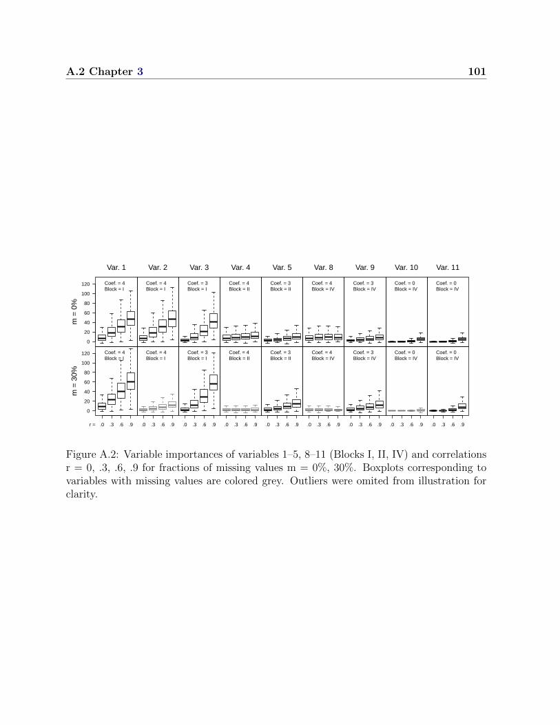
A.2 Chapter 3 101
Var. 1
Coef. = 4Block = I
0
20
40
60
80
100
120
m =
0%
Var. 2
Coef. = 4Block = I
Var. 3
Coef. = 3Block = I
Var. 4
Coef. = 4Block = II
Var. 5
Coef. = 3Block = II
Var. 8
Coef. = 4Block = IV
Var. 9
Coef. = 3Block = IV
Var. 10
Coef. = 0Block = IV
Var. 11
Coef. = 0Block = IV
.0 .3 .6 .9r =
Coef. = 4Block = I
0
20
40
60
80
100
120
m =
30%
.0 .3 .6 .9
Coef. = 4Block = I
.0 .3 .6 .9
Coef. = 3Block = I
.0 .3 .6 .9
Coef. = 4Block = II
.0 .3 .6 .9
Coef. = 3Block = II
.0 .3 .6 .9
Coef. = 4Block = IV
.0 .3 .6 .9
Coef. = 3Block = IV
.0 .3 .6 .9
Coef. = 0Block = IV
.0 .3 .6 .9
Coef. = 0Block = IV
Figure A.2: Variable importances of variables 1–5, 8–11 (Blocks I, II, IV) and correlationsr = 0, .3, .6, .9 for fractions of missing values m = 0%, 30%. Boxplots corresponding tovariables with missing values are colored grey. Outliers were omited from illustration forclarity.

102 A. Supplementary Material
0.00
0.02
0.04
0.06
0.08
0.10
0.12
m = 0%
r =
.0
m = 10% m = 20%
0
15
30
46
61
m = 30%
0.00
0.02
0.04
0.06
0.08
0.10
0.12
r =
.3
0
15
30
46
61
0.00
0.02
0.04
0.06
0.08
0.10
0.12
r =
.6
0
15
30
46
61
4 4 3 4 3 4 3 4 3 0 0 2 2 0 0Coef.1 2 3 4 5 6 7 8 9 10 11 12 13 14 15Var.I I I II II III III IV IV IV IV V VI VII VIIIBlock
0.00
0.02
0.04
0.06
0.08
0.10
0.12
r =
.9
4 4 3 4 3 4 3 4 3 0 0 2 2 0 01 2 3 4 5 6 7 8 9 10 11 12 13 14 15I I I II II III III IV IV IV IV V VI VII VIII
4 4 3 4 3 4 3 4 3 0 0 2 2 0 01 2 3 4 5 6 7 8 9 10 11 12 13 14 15I I I II II III III IV IV IV IV V VI VII VIII
4 4 3 4 3 4 3 4 3 0 0 2 2 0 01 2 3 4 5 6 7 8 9 10 11 12 13 14 15I I I II II III III IV IV IV IV V VI VII VIII
0
15
30
46
61
Figure A.3: Variable importances (left axis) of block I–VIII and correlations r = 0, .3, .6,.9 for fractions of missing values m = 0%, 10%, 20%, 30% in the MAR(rank) setting andclassification problem. Boxplots of variables that contain missing values are colored grey.Horizontal lines indicate selection frequencies (right axis). Vertical dashed lines indicatecorrespondance to the same block. Outliers are omitted from illustration for clarity.

A.3 Chapter 4 103
A.3 Chapter 4
Figure A.4 displays median importance measures observed for the regression problem.
MCAR
0.0
0.5
1.0
1.5
2.0
2.5 MAR(rank)
m = 0.0 0.1 0.2 0.3
MAR(median)
MAR(upper)
0.0
0.5
1.0
1.5
2.0
2.5
2 2 0 0 2 01 2 3 4 5 6
Coef.Var.
MAR(margins)
2 2 0 0 2 01 2 3 4 5 6
MNAR(upper)
2 2 0 0 2 01 2 3 4 5 6
impo
rtan
ce
(a) new importance measure
MCAR
0.0
0.5
1.0
1.5 MAR(rank)
m = 0.0 0.1 0.2 0.3
MAR(median)
MAR(upper)
0.0
0.5
1.0
1.5
2 2 0 0 2 01 2 3 4 5 6
Coef.Var.
MAR(margins)
2 2 0 0 2 01 2 3 4 5 6
MNAR(upper)
2 2 0 0 2 01 2 3 4 5 6
impo
rtan
ce
(b) complete case analysis
MCAR
0.0
0.5
1.0
1.5 MAR(rank)
m = 0.0 0.1 0.2 0.3
MAR(median)
MAR(upper)
0.0
0.5
1.0
1.5
2 2 0 0 2 01 2 3 4 5 6
Coef.Var.
MAR(margins)
2 2 0 0 2 01 2 3 4 5 6
MNAR(upper)
2 2 0 0 2 01 2 3 4 5 6
impo
rtan
ce
(c) multiple imputation
Figure A.4: Median variable importance observed for the regression problem (m = % ofmissing values in X2, X4 and X5).
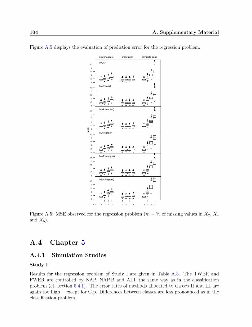
104 A. Supplementary Material
Figure A.5 displays the evaluation of prediction error for the regression problem.
●●●●
●●●●●● ●
●
●●●●●●
●●●●●●●
●●●●●
●●●●●●●●●● ●●
●
●
●
●●●●●●●
●●●●●●●●●●
●●
●
●●●●●● ●●●
●●●●●●●
●●
●●
●
●●
●
●
●
●
●
●
●●
●
●●●
●●●
●
●●●●●●●●●●●●●●●●●
●
●●●●●
●
●●
●●●
●●●●
●●
●●●●●●●●●●●●●●●
●
●
●●●
●
●
●●
●●●
●
●
●●●●●
●●
●●●●●●
●
●●●
1
1.5
2
2.5
3
3.5MCAR
new measure complete caseimputation
●●●●
●●●●●●
●●●●●
●
●
●●
●
●
●●●
●●
●
●
●
●●●●●●●●●●
●●●●●●●
●●●●●● ●
●●●
●●●
●●
●●●●●●●
●
●●●
●
●●●●●●●●●●
●●
●
●●●●●
●●●●●●●●●●●
●
●
●
●
●
●●
●●
●
●●
●
●●●
●
●
●
●
●
●
●
●
●
●
●
●
●●
●
●
●●
●●●●●●●
●
●
●
●●●●
●
●
●
●●●●●●
●
●●
●
●
●
●
●
●
●●●
●
●●
●●●●●
●
●
1
1.5
2
2.5
3
3.5MAR(rank)
●●●●
●●●●●● ●
●
●●●
●●●
●●●●●
●●
●
●●
●
●
●●●●●●●●●●
●●●
●
●●●●●●●●
●●●●●●●●● ●●
●●●●
●●●●●●●●●●
●
●
●
●●●
●●●
●
●●●●
●
●●●●
●
●●
●
●
●
●
●
●
●
●
●
●
●
●
●
●
●
●
●
●
●
●●
●
●
●●●
●
●
●
●
●●
●
●
●
●●
●
●●
●
●●
●●
●
●
●
●
●
●
●●●
●
●
●●
●
●
●●
●
●
●
1
1.5
2
2.5
3
3.5MAR(median)
●●●●
●●●●●●
●●●●●●●
●●●●●●●●
●
●
●
●●
●●●●●●●●●●
●●●●
●
●●●●●
●●●
●●●●●●●●●
●●●● ●●●●
●
●●●●●●●●●●●●●●
●●
●
●●
●
●
●●●●●●●●
●●
●●
●
●
●●
●
●
●
●
●
●
●
●
●●
●
●
●●
●
●●
●
●
●
1
1.5
2
2.5
3
3.5MAR(upper)
●●●●
●●●●●● ●●
●●●●●●●●●
●●
●●
●●
●
●●
●●●●
●
●●
●●●●●●
●●●●●●●●●●
●●●●●●●●●●
●●●●●●●●●●●
●●●●●●●●●●● ●●●
●●●●●●●
●
●
●●●●
●
●●●
●
●
●●●●
●
●●
●●●●●●●●●
●
●
●●●●
●●
●
●
●
●●
●
●●●
●
●
●
●
●
●●●●
●
●
●●
●●
●●●●●●
●
●
●
●
1
1.5
2
2.5
3
3.5MAR(margins)
●●●●
●●●●●●
●
●
●●●●●
●●
●●●
●●
●●●
●
●
●
●●
●●●●●●●●●● ●●
●
●●●●●●● ●●●●●
●●●●●●●
●●●●●●●
●●
●●●●
●
●●●●●●
●●●●●●●●●●
●●●●●●●●
●
●
●
●●
●●
●●
●●
●●
●
●
●
●
●●●
●
●
●
●
●●
●
●
●
●
●
●
●
1
1.5
2
2.5
3
3.5MNAR(upper)
.0 .1 .2 .3 .0 .1 .2 .3 .0 .1 .2 .3m =
MS
E
Figure A.5: MSE observed for the regression problem (m = % of missing values in X2, X4
and X5).
A.4 Chapter 5
A.4.1 Simulation Studies
Study I
Results for the regression problem of Study I are given in Table A.3. The TWER andFWER are controlled by NAP, NAP.B and ALT the same way as in the classificationproblem (cf. section 5.4.1). The error rates of methods allocated to classes II and III areagain too high – except for G.p. Differences between classes are less pronounced as in theclassification problem.

A.4 Chapter 5 105
TWER FWER Classvar. 1 var. 2 var. 3 var. 4 var. 5
NAP.B 1.0% 0.8% 1.0% 1.1% 1.1% 4.8% INAP 5.2% 4.7% 5.5% 5.4% 4.8% 22.6% IALT 4.8% 5.1% 5.4% 5.2% 5.1% 23.4% IG.p 1.2% 1.5% 2.0% 1.4% 1.6% 6.2% IID.1 13.6% 13.6% 14.6% 13.7% 13.6% 27.9% IIJ.1 13.7% 13.9% 14.1% 14.4% 13.9% 29.3% IIG.i 10.2% 9.9% 10.5% 10.7% 10.5% 25.0% IIJ.0 13.7% 13.9% 14.1% 14.4% 13.9% 29.3% IIID.0 13.6% 13.6% 14.6% 13.7% 13.6% 27.9% IIISVT 20.0% 19.9% 20.5% 20.1% 20.0% 25.3% III
Table A.3: TWER and FWER for 5000 simulation runs of the regression problem instudy I. Approaches are ranked and allocated to classes according to the results of theclassification problem.
Study II
The following contains – in addition to the findings and conclusions already presented insection 5.4.1 – an extensive discussion of the performance of single approaches in StudyII. For an improved clarity of presentation, Figure A.6 consists of two columns separatingapproaches which produce low to moderate TWER (class I and II) from those which showedan extremely increased TWER (class III). The new approaches are compared against eachof them.
The left column of Figure A.6 displays results for J.0, D.0 and SVT. The horizontal graylines indicate a selection frequency of 50 which is expected to be reached when the TWERof a non-relevant variable equals 5%. An examination of results for variable 6 makes clearthat J.0, D.0 and SVT select this non-relevant variable far too often. The same holds forvariable 1, 3 and 5 which are also of no relevance when s = 0. Consequently it is notsurprising that these approaches – besides this tendency to select non-relevant variables– also show a high power to detect relevant ones. Thus, variables 1, 2 and 3 for s > 0as well as variable 4 and variable 5 (which is correlated to the informative variable 3) arefrequently selected by these approaches. SVT slightly outperforms J.0 and D.0 as it showsfewer false discoveries and a higher power as s increases. It is also interesting to note thatthe selection frequency of the relevant variable 4 even drops for J.0 and D.0 with a risingrelevance of variables 1, 2 and 3 (s > 0). In summary the approaches seem to be capableto detect relevant variables with a high power. However, this is not a big achievement asit comes at the cost of a high TWER. More surprisingly the new approaches NAP andNAP.B show competitive and in some cases even superior results though they control theTWER – or even the FWER (which holds for NAP.B). The latter property is shown byselection frequencies of variable 6 as well as variables 1, 3 and 5 when s = 0. In terms

106 A. Supplementary Material
of informative variables NAP is even able to outperform its competitors (c.f. variable 2and 4) while it is not inferior in any other case. Even the by definition more conservativeNAP.B shows competitive results when s increases.
The right column of Figure A.6 displays results for J.1, D.1, ALT, G.i and G.p. Aninvestigation of selection frequencies of variable 6 as well as variables 1, 3 and 5 when s = 0makes clear that the approaches – except for a slight violation by G.i – do not exceed thethreshold TWER (gray line). In regard of the relevant variables 1, 2, 3, 4 and 5 (s > 0) theapproaches NAP, NAP.B, ALT and G.i clearly perform best – though there is always one ofthe latter two that shows inferior results for some of the variables. NAP.B is only slightlyinferior to NAP. It often outperforms or compares to ALT and G.i though it is expectedto be more conservative (as it is the only approach that controls the FWER). NAP – andNAP.B for larger values of s – are the only approaches which are able to detect variable5 which is of relevance as it is correlated to the informative variable 3. J.1, D.1 and G.pshow inferior results throughout. For these approaches and G.i the selection frequency ofthe informative variable 4 even decreases with a rising strength of variables 1, 2 and 3(s > 0); while it stays constant for approaches of class I (i.e. NAP, NAP.B and ALT).
NAP shows the highest power and clearly outperforms ALT – which is of major interestas both methods only slightly differ, yet in a substantial aspect of the permutation scheme.A discussion in section 5.2.3 already outlined that this is because the empirical distributionof importances of relevant variables has higher upper percentiles under H∗0 (5.2) – followedby ALT – than under H0 (5.1) – followed by NAP. Therefore NAP is able to reject thenull-hypothesis for relevant variables, that initially have an importance score of a certainmagnitude, more often.
Results for the regression problem are similar, yet they stress the superiority of thenew approaches even stronger (cf. Figure A.7). NAP and NAP.B clearly outperform theircompetitors as they show the highest discriminatory power in this case.
Study III
In relation to section 5.4.1 a much more detailed illustration of the results for each approachin study III is given by Figure A.8. A comparison to the approaches G.i, G.p, J.1, D.1and ALT reveals a clear superiority of NAP and NAP.B in terms of the ability to identifyrelevant variables. In analogy to the findings of Study II the only approach which is ableto keep up – now in a setting of a simulated data set – is ALT. However, it is outperformedby NAP – which it resembles the most (cf. section 5.2.3 for a discussion about the reasonsbehind this superiority of NAP) – and only compares to NAP.B though the latter is – bydefinition – much more conservative as it uses the Bonferroni-Adjustment. A comparisonto J.0, D.0 and SVT reveals that these approaches again produce error rates far beyondthe 5% level. Still they are not able to clearly outperform NAP and NAP.B, especially forhigher values of s.
The superiority of the new approaches becomes even more evident in the regressionproblem (cf. Figure A.9): they show the highest power to detect relevant variables, the

A.4 Chapter 5 107
0
200
400
600
800
1000
sel.
freq
.
NAPJ.0SVT
NAP.BD.0
var. 1
NAPJ.1G.pG.i
NAP.BD.1ALT
0
200
400
600
800
1000
sel.
freq
.
var. 2
0
200
400
600
800
1000
sel.
freq
.
var. 3
0
200
400
600
800
1000
sel.
freq
.
var. 4
0
200
400
600
800
1000
sel.
freq
.
var. 5
0
200
400
600
800
1000
0 0.1 0.2 0.3 0.4 0.5 0.6 0.7 0.8 0.9 1s =
sel.
freq
.
0 0.1 0.2 0.3 0.4 0.5 0.6 0.7 0.8 0.9 1
var. 6
Figure A.6: Plot of selection frequencies in 1000 simulation runs of the classification prob-lem of study II. Results are shown in dependence of predictor strength as determined byβII = (s, s, s, 1, 0, 0)>. There are no relations except for pairwise correlations (r = 0.7)between variable 2 and 4 as well as 3 and 5. Comparisons of the new approaches to classIII and II (+ ALT) are given in the left and right column, respectively. The horizontal linerepresents a 5% TWER. [Relevant Variables: var. 4 & var. 1 – 3, 5 for s > 0; InformativeVariables: var. 4 & var. 1 – 3 for s > 0]
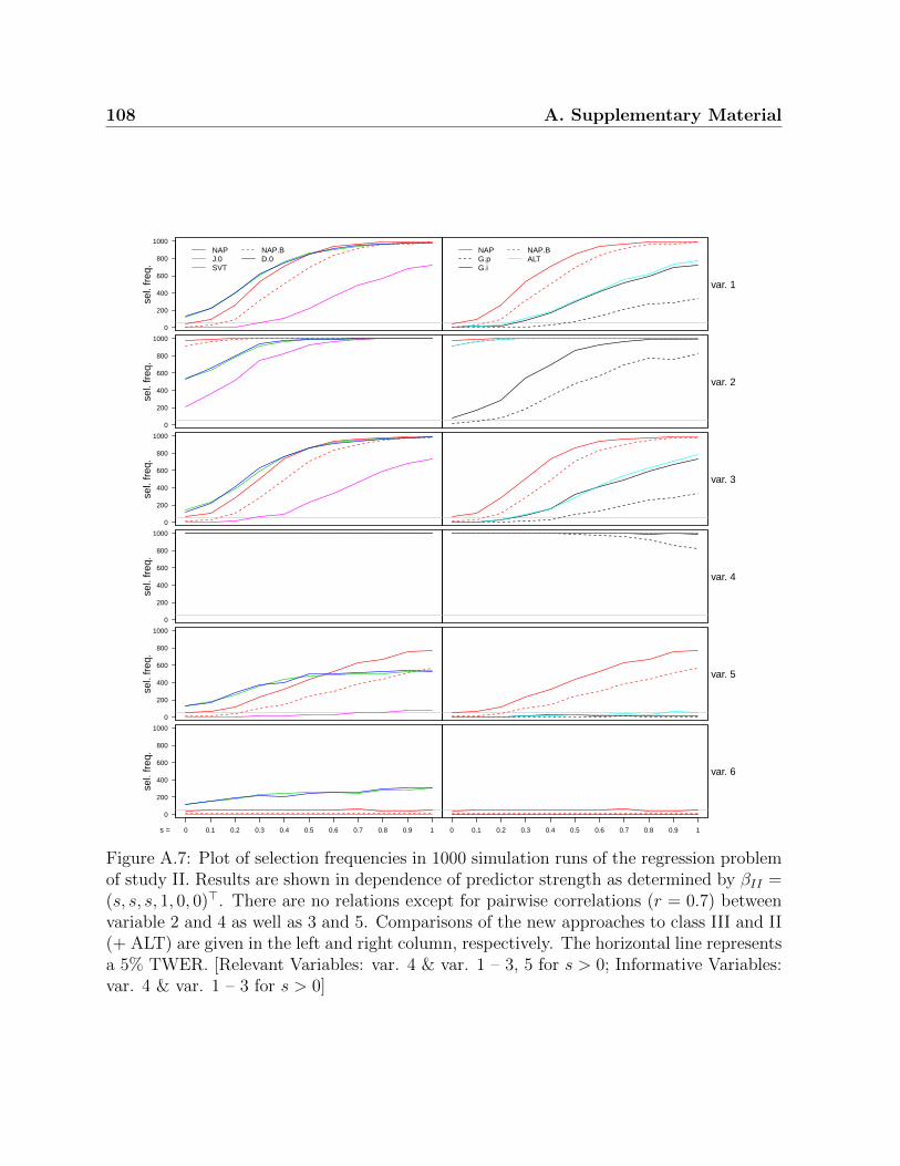
108 A. Supplementary Material
0
200
400
600
800
1000
sel.
freq
.
NAPJ.0SVT
NAP.BD.0
var. 1
NAPG.pG.i
NAP.BALT
0
200
400
600
800
1000
sel.
freq
.
var. 2
0
200
400
600
800
1000
sel.
freq
.
var. 3
0
200
400
600
800
1000
sel.
freq
.
var. 4
0
200
400
600
800
1000
sel.
freq
.
var. 5
0
200
400
600
800
1000
0 0.1 0.2 0.3 0.4 0.5 0.6 0.7 0.8 0.9 1s =
sel.
freq
.
0 0.1 0.2 0.3 0.4 0.5 0.6 0.7 0.8 0.9 1
var. 6
Figure A.7: Plot of selection frequencies in 1000 simulation runs of the regression problemof study II. Results are shown in dependence of predictor strength as determined by βII =(s, s, s, 1, 0, 0)>. There are no relations except for pairwise correlations (r = 0.7) betweenvariable 2 and 4 as well as 3 and 5. Comparisons of the new approaches to class III and II(+ ALT) are given in the left and right column, respectively. The horizontal line representsa 5% TWER. [Relevant Variables: var. 4 & var. 1 – 3, 5 for s > 0; Informative Variables:var. 4 & var. 1 – 3 for s > 0]

A.4 Chapter 5 109
sel.
freq
.
0
200
400
600
800
1000
3 2 1 (3 2 1) (3 2 1 0 0) (0 0) 0 01 2 3 4 5 6 7 8 9 10 11 12 13 14 15var. =
coef. =
(a)
NAPNAP.BJ.0D.0SVT
sel.
freq
.
0
200
400
600
800
1000
3 2 1 (3 2 1) (3 2 1 0 0) (0 0) 0 01 2 3 4 5 6 7 8 9 10 11 12 13 14 15var. =
coef. =
(b)
NAPNAP.BG.iG.pJ.1D.1ALT
●●●
●
●●●
●
●●●●●●●●●● ●
●●●●
●●
●
●●
●●●●●●●●●●●●●
●●
●●
●
●●●
●
●
●●●●
●●
●
●
●●●●
●●
●●
●
●
●
●
●
●
●●●
●
●●●●●●●●●●●●
●
●
●
●
●
●
●
●
●
●
●
●
●●
●
●
●●
●
●●
●
●
●●●
●
●●●●●●●●●
●●
●●●
●
●
●
●
●●
●
●●●
●●●
●●
●●
●
●●●●●●
●●●●●●
●●
●●●●●
●●●●●●
●
●●●●●
●
●●●●●●
●
●●●●●
●●●●
●
●●●●●●●●●●
●●●●
●
●
●
●●
●●●
●
All NAP SVT D.0 ALT J.0 NAP.B G.i D.1 J.1 G.p
0.10
0.15
0.20
0.25
0.30
0.35
0.40
0.45
MS
E
(c)
0.188 0.192 0.194 0.201 0.202 0.202 0.204 0.215 0.218 0.221 0.251med. =
All NAP SVT D.0 ALT J.0 NAP.B G.i D.1 J.1 G.p
mea
n se
l. fr
eq.
0
5
10
15
20
(d)
20
9.210.7 10.7
6.7
10.1
6.54.7 5 4.3
2.4
118.8 9 8.2
6.7 7.76.4
4.7 4.7 4.22.4
97 7.3 6.8
5.6 6.4 5.44.3 4.2 3.8
2.2
var. selected # relevant # informative
Figure A.8: Selection frequencies of variables 1-15 in 1000 simulation runs of the classifi-cation problem of study III. The new approaches are compared to class III (a) and classII (+ ALT) (b). The horizontal grey line represents a 5% TWER. Brackets indicate corre-lated variables. (c) Boxplots of the observed MSE aranged in increasing order of medianvalues. (d) Mean selection frequency of variables and an additional information about theamount of relevant and informative variables among them. Reference values are indicatedby horizontal lines. [Relevant Variables: var. 1 – 11; Informative Variables: var. 1 – 9]

110 A. Supplementary Material
sel.
freq
.
0
200
400
600
800
1000
3 2 1 (3 2 1) (3 2 1 0 0) (0 0) 0 01 2 3 4 5 6 7 8 9 10 11 12 13 14 15var. =
coef. =
(a)
NAPNAP.BG.iG.pJ.0D.0ALTSVT
●●
●●●
●●●●●●●●●
● ●●
●●●●●●●●
●
●●●●●●●●
●
●
●●●
●
●●
●●●
●●
●●●●●
●
●●●
●
●
●
●
●●●●●
●
●●●●●●●●●●●●
●
●
●●
●●
●●●
●
●●
●●
●
●
●
●
●●●
●
●
●
●●●
●●
●
●
●
●
●●●
●
●●●
●
●
●
●●
●
●
●
●
●
●
●
●
●
●●
●
●●●●●
●
●●
●
●
●●
●
●
●
●
●
●
●
●
●
●
●●
●
●
●
●
●
●
●
●
●
●
●●
●
●
●
●
●
●●
●●
●
●
●
●●
●
●●●
●●
●
●●
●
●
●
●
●
●
●
●●
●
●
●●
●
●●
●
●
●●●
●
●
●
●
●●
●
●
●
●
NAP NAP.B ALT All SVT G.i J.1 D.1 G.p
20
30
40
50
60
MS
E
(b)
29.62 29.63 29.84 30.5 32.9 33.11 33.89 34.13 34.82med. =
NAP NAP.B ALT All SVT G.i J.1 D.1 G.p
mea
n se
l. fr
eq.
0
5
10
15
20
(c)10.2
8.8 8.2
20
7.3
4.3
8.6 8.9
2.7
9.88.8 8.2
11
7.3
4.3
7.7 8
2.7
7.87 6.5
9
6.1
4.1
6.5 6.7
2.6
var. selected # relevant # informative
Figure A.9: Selection frequencies of variables 1-15 in 1000 simulation runs of the regressionproblem of study III. The new approaches are compared to class III (a) and class II (+ALT) (b). The horizontal grey line represents a 5% TWER. Brackets indicate correlatedvariables. (c) Boxplots of the observed MSE aranged in increasing order of median values.(d) Mean selection frequency of variables and an additional information about the amountof relevant and informative variables among them. Reference values are indicated byhorizontal lines. [Relevant Variables: var. 1 – 11; Informative Variables: var. 1 – 9]
lowest median MSE and the highest effectiveness while the efficiencies are among thehighest, too.
A.4.2 Empirical Evaluation
In addition to the findings of section 5.4.2 Table A.4 contains the selection frequencies ofvariables which were observed for the empirical evaluation within 1000 bootstrap runs.

A.4 Chapter 5 111
Variable NAP NAP.B G.i G.p J.0 J.1 D.0 D.1 ALT SVT
Birthweight low 1000 1000 1000 1000 1000 1000 1000 1000age 907 553 7 0 658 612 255 3lwt 990 922 214 1 920 924 783 72
race 967 861 0 0 791 826 759 10smoke 987 917 0 0 808 839 836 5
ptl 576 323 0 0 47 98 274 0ht 353 208 0 0 26 34 175 0ui 975 883 0 0 654 731 875 1
ftv 498 137 0 0 102 112 30 0
B. Housing CRIM 1000 1000 135 14 979 957 999 107ZN 969 860 0 0 65 105 73 0
INDUS 1000 1000 69 1 813 910 996 224CHAS 859 698 0 0 43 50 169 0NOX 1000 1000 226 57 958 970 997 92
RM 1000 1000 1000 999 1000 1000 1000 1000AGE 1000 1000 0 0 636 657 648 0DIS 1000 1000 1 0 757 745 699 2
RAD 1000 1000 0 0 405 411 515 0TAX 1000 1000 5 0 862 853 997 29
PTRATIO 1000 1000 191 18 909 955 1000 326B 1000 1000 0 0 385 397 298 0
LSTAT 1000 1000 1000 1000 1000 1000 1000 1000
Heart age 917 724 83 5 628 161 672 182 253 761sex 993 932 233 25 768 306 825 358 647 882cp 1000 999 985 448 991 944 995 954 994 999
trestbps 765 435 50 1 486 96 501 95 62 586chol 761 452 68 2 544 128 547 107 83 663fbs 296 90 1 0 183 12 201 13 1 175
restecg 725 423 50 3 525 121 515 122 97 582thalach 1000 997 464 119 878 531 902 587 905 958
exang 995 977 361 59 849 476 875 504 843 932oldpeak 999 996 609 192 908 682 948 708 959 972
slope 984 917 310 44 777 366 810 391 701 907ca 1000 1000 991 450 998 984 998 985 1000 1000
thal 1000 1000 982 643 996 977 997 987 1000 999
Parkinson MDVP.Fo.Hz. 995 950 681 147 863 577 887 558 922 845MDVP.Fhi.Hz. 962 708 241 15 634 277 629 222 451 506MDVP.Flo.Hz. 966 745 212 29 565 159 657 242 554 585MDVP.Jitter... 572 98 0 0 140 3 206 15 9 187
MDVP.Jitter.Abs. 940 653 55 5 401 59 529 113 369 408MDVP.RAP 595 167 5 0 177 15 242 25 28 212MDVP.PPQ 599 138 1 0 153 6 208 24 13 207Jitter.DDP 590 183 11 0 187 17 248 33 33 231
MDVP.Shimmer 991 897 353 34 649 242 752 322 759 645MDVP.Shimmer.dB. 923 590 80 0 390 73 513 131 376 436
Shimmer.APQ3 965 702 121 2 540 160 617 189 402 484Shimmer.APQ5 964 754 188 11 498 129 643 236 534 536
MDVP.APQ 988 907 326 33 594 189 744 334 670 661Shimmer.DDA 973 738 153 9 592 194 636 202 452 522
NHR 455 86 5 0 128 4 155 15 4 146HNR 931 598 112 15 493 125 567 160 244 454
RPDE 888 464 63 4 463 158 508 129 183 393DFA 847 378 67 4 399 77 435 108 224 336
spread1 1000 1000 957 880 992 982 977 916 1000 994spread2 995 980 632 140 810 439 879 595 951 861
D2 955 759 349 62 623 253 688 325 617 576PPE 1000 1000 898 541 936 760 967 857 1000 988
Table A.4: Summary of variable selection frequencies observed for 1000 bootstrap runs ofthe empirical evaluation.

112 A. Supplementary Material
A.5 Chapter 6
Results for the regression problem are presented in Figure A.10. They underline the find-ings for the classification problem. The 0 s.e. rule was executed for the performance-basedapproach. As a consequence, its TWER and selection frequencies are increased.
● ● ● ● ● ● ● ●
● ● ● ●
● ● ● ● ● ● ● ●
● ● ● ●0200400600800
1000
.0 .1 .2 .3 .0 .1 .2 .3 .0 .1 .2 .3 .0 .1 .2 .3 .0 .1 .2 .3 .0 .1 .2 .3m =
MC
AR
● test−based ( performance−based (● contains missings) contains missings)
● ● ● ● ● ● ● ●
● ● ● ●
● ● ● ● ● ● ●●
● ● ● ●0200400600800
1000
MA
R(r
ank)
● ● ● ● ● ● ● ●
● ● ● ●
● ● ● ● ● ● ● ●
● ● ● ●0200400600800
1000
MA
R(m
edia
n)
● ● ● ● ● ● ● ●
● ● ● ●
● ● ● ● ● ● ● ●
● ● ● ●0200400600800
1000
MA
R(u
pper
)
● ● ● ● ● ● ● ●
● ● ● ●
● ● ● ● ● ● ● ●
● ● ● ●0200400600800
1000
MA
R(m
argi
ns)
● ● ● ● ● ● ●●
● ● ● ●
● ● ● ● ● ●●
●
● ● ● ●0200400600800
1000
1 2 3 4 5 6variable
MN
AR
(upp
er)
sele
ctio
n fr
eque
ncy
(a) new importance measure
● ● ● ● ● ● ● ●
● ● ● ●
● ● ●●
● ● ●●
● ● ● ●0200400600800
1000
.0 .1 .2 .3 .0 .1 .2 .3 .0 .1 .2 .3 .0 .1 .2 .3 .0 .1 .2 .3 .0 .1 .2 .3m =
MC
AR
● test−based ( performance−based (● contains missings) contains missings)
● ● ● ● ● ● ● ●
● ● ● ●
● ● ●●
● ● ●●
● ● ● ●0200400600800
1000
MA
R(r
ank)
● ● ● ● ● ● ● ●
● ● ● ●
● ● ●
●
● ● ●●
● ● ● ●0200400600800
1000
MA
R(m
edia
n)● ● ●
●● ● ● ●
●● ● ●
● ●●
●
● ● ● ●
● ● ● ●0200400600800
1000M
AR
(upp
er)
● ●●
●
● ● ● ●
●● ● ●
● ●
●
●
● ● ● ●
● ● ● ●0200400600800
1000
MA
R(m
argi
ns)
● ● ● ● ● ● ●●
●●
● ●
● ● ● ●● ●
●
●
● ● ● ●0200400600800
1000
1 2 3 4 5 6variable
MN
AR
(upp
er)
sele
ctio
n fr
eque
ncy
(b) complete case analysis
● ● ● ● ● ● ● ●
● ● ● ●
● ● ● ● ● ● ● ●
● ● ● ●0200400600800
1000
.0 .1 .2 .3 .0 .1 .2 .3 .0 .1 .2 .3 .0 .1 .2 .3 .0 .1 .2 .3 .0 .1 .2 .3m =
MC
AR
● test−based ( performance−based (● contains missings) contains missings)
● ● ● ● ● ● ● ●
● ● ● ●
● ● ● ● ● ● ● ●
● ● ● ●0200400600800
1000
MA
R(r
ank)
● ● ● ● ● ● ● ●
● ● ● ●
● ● ● ● ● ● ● ●
● ● ● ●0200400600800
1000
MA
R(m
edia
n)
● ● ● ● ● ● ● ●
● ● ● ●
● ● ● ● ● ● ● ●
● ● ● ●0200400600800
1000
MA
R(u
pper
)
● ● ● ● ● ● ● ●
● ● ● ●
● ● ● ● ● ● ● ●
● ● ● ●0200400600800
1000
MA
R(m
argi
ns)
● ● ● ● ● ● ● ●
● ● ● ●
● ● ● ● ● ● ●●
● ● ● ●0200400600800
1000
1 2 3 4 5 6variable
MN
AR
(upp
er)
sele
ctio
n fr
eque
ncy
(c) multiple imputation
1
2
3
4
5
6 MCAR
new measure imputation complete case
test−based performance−based
1
2
3
4
5
6 MAR(rank)
1
2
3
4
5
6 MAR(median)
1
2
3
4
5
6 MAR(upper)
1
2
3
4
5
6 MAR(margins)
1
2
3
4
5
6 MNAR(upper)
.0 .1 .2 .3 .0 .1 .2 .3 .0 .1 .2 .3m =
MS
E
(d) MSE
Figure A.10: Variable selection frequencies and MSE observed for the regression problem(m = % of missing values in X2 and X5).

Appendix B
R-Code
All of this works computations are operable by the following Code using R (version 2.14.1).General functions used throughout the studies are:
# Function to count selection frequencies of variables in Random Forests
count <- function(forest, inames = NULL) {
# forest: object of class "RandomForest" created by the function cforest()
# inames: names of variables to be assessed (defaults to NULL, using all variables)
if (is.null(inames) && extends(class(forest), "RandomForest"))
inames <- names(forest@data@get("input"))
resultvec <- rep(0, length(inames))
myfunc <- function(x, inames, resultvec) {
names(x) <- c("nodeID", "weights", "criterion", "terminal", "psplit",
"ssplits", "prediction", "left", "right")
names(x$criterion) <- c("statistic", "criterion", "maxcriterion")
if (!x$terminal) {
resultvec[x$psplit[[1]]] <- resultvec[x$psplit[[1]]] + 1
resultvec <- myfunc(x$left, inames = inames, resultvec = resultvec)
resultvec <- myfunc(x$right, inames = inames, resultvec = resultvec)
}
return(resultvec)
}
for (k in 1:length(forest@ensemble)) {
resultvec <- myfunc(forest@ensemble[[k]], inames, resultvec)
}
names(resultvec) <- inames
return(resultvec)
}
environment(count) <- environment(varimp)
# Function to simulate data
create.dat <- function(coefs = c(0, 0, 0, 0, 0), n = 100,
sigma = NULL, regression = T, error = 1) {
# coefs: coefficients; n: number of observations; sigma: covariance matrix
# regression: TRUE produces a regression problem, FALSE a classification problem
# error: error added to outcome in case of a regression problem
if (is.null(sigma)) sigma <- diag(length(coefs)) # initialize sigma

114 B. R-Code
if (length(coefs) != nrow(sigma)) stop("dimension of coefs and sigma differs")
dat <- rmvnorm(n, sigma = sigma) # create covariates
x.beta <- dat %*% coefs
dat <- as.data.frame(dat)
if (regression == T) dat$response <- x.beta + rnorm(n, 0, error) # create the response
else dat$response <- as.factor(rbinom(n, 1, exp(x.beta) / (1 + exp(x.beta))))
return(dat)
}
# Function to induce missing values into a data set
with.missings <- function(data, mis.var, ind.var, m) {
# data: data meant to contain missing values
# mis.var: names of variables to be partly set missing
# ind.var: variables that induce the missing values
# m * 10: fraction of missing values in %
X <- lapply(1:6, function(x) data) # for 6 missing data generating processes
n <- nrow(data)
for (k in mis.var) {
ind <- ind.var[mis.var == k]
# induce missing values MCAR
is.na(X[[1]][,k])[sample(1:n, m * .1 * n)] <- TRUE
# induce missing values MAR(rank)
is.na(X[[2]][,k])[sample(1:n, m * .1 * n, prob = rank(X[[2]][,ind]) / sum(1:n))] <- TRUE
# induce missing values MAR(median)
is.na(X[[3]][,k])[sample(1:n, m * .1 * n, prob = ifelse(X[[3]][,
ind] >= median(X[[3]][,ind]), .9, .1))] <- TRUE
# induce missing values MAR(upper)
is.na(X[[4]][,k])[X[[4]][,ind] >= sort(X[[4]][,ind], T)[m * .1 * n]] <- TRUE
# induce missing values MAR(margins)
is.na(X[[5]][,k])[X[[5]][,ind] >= sort(X[[5]][,ind], T)[m * .1 * n / 2] |
X[[5]][,ind] <= sort(X[[5]][,ind])[m * .1 * n / 2]] <- TRUE
# induce missing values MNAR(upper)
is.na(X[[6]][,k])[X[[6]][,k] >= sort(X[[6]][,k], T)[m * .1 * n]] <- TRUE
}
return(X)
}
B.1 Chapter 1
The following code gives a short summary of how to create and display trees and RandomForests. Further functionalities are given by manuals of the packages party and rpart.Also, steps to create figures and views can be taken from any R-Code textbook and are notpresented here.
set.seed(290875) # set a random seed for reproducibility of results
# load the airquality data and reject observations with missing response
airq <- subset(airquality, !is.na(Ozone))

B.2 Chapter 2 115
library(party) # load required package ‘party’ version 1.0-0
airct <- ctree(Ozone ~ ., data = airq, # create a tree with 3 surrogates
controls = ctree_control(maxsurrogate = 3))
airct # display it
plot(airct) # and plot it
library(rpart) # load required package ‘rpart’ version 3.1-52
aircart <- rpart(Ozone ~ ., data = airq) # create a CART like tree
printcp(aircart) # assess the cross-validated error for different tree sizes
aircart.pruned <- prune(aircart, cp = 0.08) # prune the tree to the optimal size
plot(aircart.pruned); text(aircart.pruned) # plot the tree
aircf <- cforest(Ozone ~ ., data = airq) # create a Random Forest
count(aircf) # apply the count() function
airq2 <- na.omit(airquality) # create a complete case version of the data
aircf2 <- cforest(Ozone ~ ., data = airq2) # and a corresponding Random Forest
# compute the permutation importance measure and its conditional version
varimp(aircf2, pre1.0_0 = T); varimp(aircf2, conditional = T)
B.2 Chapter 2
B.2.1 Simulation Studies
R-Code used for the simulation studies by the example of Haberman’s Survival Data (otherdatasets were processed the same way):
# load required packages
library(party) # version 1.0-0
library(mice) # version 2.11
library(rpart) # version 3.1-52
# define the predictors used in the imputation models
predmat <- matrix(1, ncol = 4, nrow = 4); diag(predmat) <- 0; predmat[, 4] <- 0
repetitions <- 1000 # there were 1000 MCCV runs
# create matrices that take the observed MSE values for Random Forests, conditional
# inference trees (=tree) and CART (=oldtree). "with" = imputation was used
mse.without.forest <- mse.with.forest <- mse.without.tree <- mse.with.tree <-
mse.without.oldtree <- mse.with.oldtree <- matrix(NA, nrow = 4, ncol = repetitions,
dimnames = list(seq(.1, .4, .1), 1:repetitions))
# load the data
dat <- read.table("your_local_directory/haberman.txt", sep = ",")
names(dat) <- c("age", "year", "nodes", "surv")
dat$surv <- as.factor(dat$surv)
for (j in 1:4) { # there are four fractions of missing values
for (i in 1:repetitions) { # and 1000 repetitions
misdat <- dat

116 B. R-Code
miss <- sapply(1:3, function(x) sample(1:nrow(misdat), round(nrow(misdat)* 0.1 * j)))
for (k in 1:3) {is.na(misdat[miss[, k], k]) <- T}
### when only 1/3 of variables should contain missing values, use instead:
#miss <- sample(1:nrow(misdat), round(nrow(misdat)* 0.1 * j))
#is.na(misdat[miss, sample(1:3, 1)]) <- T
# samples are drawn to build the training and test data
samp <- sample(1:nrow(misdat), round(nrow(misdat) * .8), replace = F)
dat.train <- misdat[samp, ]; dat.test <- misdat[-samp, ]
# use MICE to impute the data
test.mi <- mice(dat.test, printFlag = F, defaultMethod = c("norm", "logreg", "polyreg"),
predictorMatrix = predmat)
train.mi <- mice(dat.train, printFlag = F, defaultMethod = c("norm", "logreg", "polyreg"))
# compute the MSE values without imputation
forest <- cforest(surv ~ ., data = dat.train, controls =
cforest_unbiased(maxsurrogate = min(3, ncol(dat) - 2)))
mse.without.forest[j, i] <- mean((as.numeric(dat.test$surv) -
as.numeric(Predict(forest, newdata = dat.test)))^2)
tree <- ctree(surv ~ ., data = dat.train, controls =
ctree_control(maxsurrogate = min(3, ncol(dat) - 2)))
mse.without.tree[j, i] <- mean((as.numeric(dat.test$surv) -
as.numeric(predict(tree, newdata = dat.test)))^2)
oldtree <- rpart(surv ~ ., data = dat.train)
mse.without.oldtree[j, i] <- mean((as.numeric(dat.test$surv) -
round(predict(oldtree, newdata = dat.test)[, "2"]) - 1)^2)
# compute the MSE values with imputation
mse.with.forest[j, i] <- mean((as.numeric(dat.test$surv) - round(rowMeans(sapply(1:5,
function(x) {mi.forest <- cforest(surv ~ .,
data = complete(train.mi, action = x), controls =
cforest_unbiased(maxsurrogate = min(3, ncol(dat) - 2)));
return(rowMeans(sapply(1:5, function(y)
as.numeric(Predict(mi.forest, newdata = complete(test.mi,
action = y))))))}))))^2)
mse.with.tree[j, i] <- mean((as.numeric(dat.test$surv) - round(rowMeans(sapply(1:5,
function(x) {mi.forest <- ctree(surv ~ ., data =
complete(train.mi, action = x), controls =
ctree_control(maxsurrogate = min(3, ncol(dat) - 2)));
return(rowMeans(sapply(1:5, function(y)
as.numeric(predict(mi.forest, newdata =
complete(test.mi, action = y))))))}))))^2)
mse.with.oldtree[j, i] <- mean((as.numeric(dat.test$surv) - round(rowMeans(sapply(1:5,
function(x) {mi.forest <- rpart(surv ~ ., data =
complete(train.mi, action = x));
return(rowMeans(sapply(1:5, function(y)
round(predict(mi.forest, newdata = complete(test.mi,
action = y))[, "2"]))))}))) - 1)^2)
}
}

B.2 Chapter 2 117
B.2.2 Empirical Evaluation
R-Code used for the application studies by the example of the Hepatitis Dataset (otherdatasets were processed the same way):
# load required packages
library(party) # version 1.0-0
library(mice) # version 2.11
library(rpart) # version 3.1-52
# define the predictors used in the imputation models
predmat <- matrix(1, ncol = 20, nrow = 20); diag(predmat) <- 0; predmat[, 1] <- 0
repetitions <- 1000 # there were 1000 MCCV runs
# create matrices that take the observed MSE values for Random Forests, conditional
# inference trees (=tree) and CART (=oldtree). "with" means that imputation was used
mse.ohne.forest <- mse.mit.forest <- mse.ohne.tree <- mse.mit.tree <-
mse.ohne.oldtree <- mse.mit.oldtree <- rep(NA, repetitions)
# load the data
dat <- read.table("your_local_directory/hepatitis.txt", sep = ",", na.strings = "?")
names(dat) <- c("status", "age", "sex", "steroid", "antivirals", "fatigue",
"malaise", "anorexia", "liver", "livfirm", "spleen",
"spiders", "ascites", "varices", "bilirubin", "alk", "sgot",
"albumin", "protime", "histology")
dat$status <- as.factor(dat$status)
for (i in 1:repetitions) { # there are 1000 repetitions
# samples are drawn to build the training and test data
samp <- sample(1:nrow(dat), round(nrow(dat) * .8), replace = F)
dat.train <- dat[samp, ]; dat.test <- dat[-samp, ]
# use MICE to impute the data
train.mi <- mice(dat.train, printFlag = F, defaultMethod = c("norm", "logreg", "polyreg"))
test.mi <- mice(dat.test, printFlag = F, defaultMethod = c("norm", "logreg", "polyreg"),
predictorMatrix = predmat)
# compute the MSE values without imputation
mse.ohne.forest[i] <- mean((as.numeric(dat.test$status) - as.numeric(Predict(cforest(
status ~ ., data = dat.train, controls =
cforest_unbiased(maxsurrogate = 3)), newdata = dat.test)))^2)
tree <- ctree(status ~ ., data = dat.train, controls = ctree_control(maxsurrogate = 3))
mse.ohne.tree[i] <- mean((as.numeric(dat.test$status) - as.numeric(predict(tree,
newdata = dat.test)))^2)
oldtree <- rpart(status ~ ., data = dat.train)
mse.ohne.oldtree[i] <- mean((as.numeric(dat.test$status) - round(predict(oldtree,
newdata = dat.test)[, "2"]) - 1)^2)
# compute the MSE values with imputation
mse.mit.forest[i] <- mean((as.numeric(dat.test$status) - round(rowMeans(sapply(1:5,
function(x) {mi.forest <- cforest(status ~ ., data =
complete(train.mi, action = x), controls =
cforest_unbiased(maxsurrogate = 3)); return(rowMeans(
sapply(1:5, function(y) as.numeric(Predict(mi.forest,
newdata = complete(test.mi, action = y))))))}))))^2)

118 B. R-Code
mse.mit.tree[i] <- mean((as.numeric(dat.test$status) - round(rowMeans(sapply(1:5,
function(x) {mi.forest <- ctree(status ~ ., data =
complete(train.mi, action = x), controls =
ctree_control(maxsurrogate = 3)); return(rowMeans(
sapply(1:5, function(y) as.numeric(predict(mi.forest,
newdata = complete(test.mi, action = y))))))}))))^2)
mse.mit.oldtree[i] <- mean((as.numeric(dat.test$status) - round(rowMeans(sapply(
1:5, function(x) {mi.forest <- rpart(status ~ ., data =
complete(train.mi, action = x)); return(rowMeans(sapply(
1:5, function(y) round(predict(mi.forest, newdata =
complete(test.mi, action = y))[, "2"]))))}))) - 1)^2)
}
B.3 Chapter 3
B.3.1 Simulation Studies
R-Code used for the simulation study:
# load required packages
library("party"); attach(asNamespace("party")) # version 1.0-0
library(mvtnorm) # version 0.9-9992
library(mice) # version 2.11
# create a list of covariance matrices for each correlation strength
sig <- lapply(1:4, function(x) {r <- c(0,.3,.6,.9)[x]; y <- diag(20);
y[1:3, 1:3] <- r; y[4:5, 4:5] <- r; y[6:7, 6:7] <- r;
y[8:11, 8:11] <- r; diag(y) <- 1; return(y)})
# create lists that contain arrays used to collect the results of 20 variables for 4
# fractions of missing values, 4 correlation strength and 6 missing data generating
# processes in 1000 simulation runs. The common importance measure (‘old’), the new
# approach (‘new’) and selection frequencies (‘count’) are recorded for the
# regression (‘reg’) and classification (‘clas’) problem.
reg.old <- clas.old <- reg.new <- clas.new <- reg.count <- clas.count <-
lapply(1:6, function(y) lapply(1:4, function(x) array(dim = c(1000, 20, 4))))
set.seed(1234) # set a random seed for reproducibility of results
# 1000 simulation runs start here
for (i in 1:1000) {
for (r in 1:4) { # there are 4 correlation strength
dat <- as.data.frame(rmvnorm(100, sigma = sig[[r]])) # create the data
x.beta <- with(dat, 4 * V1 + 4 * V2 + 3 * V3 + 4 * V4 + 3 * V5 +
4 * V6 + 3 * V7 + 4 * V8 + 3 * V9 + 2 * V12 + 2 * V13
dat$y.reg <- x.beta + rnorm(100, 0, .5)
dat$y.clas <- rbinom(100, 1, exp(x.beta) / (1 + exp(x.beta)))
for (m in 1:4) { # there are 4 fractions of missing values
# the data is replicated for each of 6 missing data generating process
dat.mis <- with.missings(dat, c("V2", "V4", "V8", "V10", "V12", "V14"),
c("V3", "V5", "V9", "V11", "V13", "V15"), m - 1)

B.3 Chapter 3 119
for (j in 1:6) { # compute results for 6 missing data generating processes
# create random forests and compute importances and selection frequencies
forest.reg <- cforest(as.formula(paste("y.reg", paste("V", 1:20, sep = "",
collapse = " + "), sep = " ~ ")), data = dat.mis[[j]],
controls = cforest_unbiased(mtry = 8, ntree = 50,
maxsurrogate = 3))
forest.clas <- cforest(as.formula(paste("y.clas", paste("V", 1:20, sep = "",
collapse = " + "), sep = " ~ ")), data = dat.mis[[j]],
controls = cforest_unbiased(mtry = 8, ntree = 50,
maxsurrogate = 3))
reg.new[[j]][[r]][i, , m] <- varimp(forest.reg)
clas.new[[j]][[r]][i, , m] <- varimp(forest.clas)
reg.count[[j]][[r]][i, , m] <- count(forest.reg)
clas.count[[j]][[r]][i, , m] <- count(forest.clas)
if (m == 1) {
reg.old[[j]][[r]][i, , m] <- varimp(forest.reg, pre1.0_0 = TRUE)
clas.old[[j]][[r]][i, , m] <- varimp(forest.clas, pre1.0_0 = TRUE)
}}}
}
}
B.3.2 Empirical Evaluation
R-Code used for the empirical evaluation:
# load required package
library("party"); attach(asNamespace("party")) # version 1.0-0
# load the pima indians diabetes data as provided by the UCI repository
pima <- read.table("your_local_directory/pima_data.txt", sep = ",")
names(pima) <- c("num.preg", "gluc", "bloodpres", "skin", "insulin",
"bmi", "pedigree", "age", "diabetes")
pima$diabetes <- as.factor(pima$diabetes) # prepare the data
is.na(pima$gluc[pima$gluc == 0]) <- T # and define the missing values
is.na(pima$bloodpres[pima$bloodpres == 0]) <- T
is.na(pima$skin[pima$skin == 0]) <- T; is.na(pima$bmi[pima$bmi == 0]) <- T
is.na(pima$insulin[pima$insulin == 0]) <- T
# load the mammal sleep data
slep <- read.table("your_local_directory/sleep_data.txt", header = T)
set.seed(5) # set a random seed for reproducibility of results
# create forests of 5000 trees for the pima data and the sleep data
forest.pima.new <- cforest(diabetes ~ ., controls = cforest_unbiased(mtry = 3,
maxsurrogate = 3, ntree = 5000), data = pima)
forest.sleep.new <- cforest(BodyWgt ~ ., controls = cforest_unbiased(mtry = 3,
maxsurrogate = 3, ntree = 5000), data = slep)
# create a forest of 5000 trees for a complete case versions of the data
forest.pima.old <- cforest(diabetes ~ ., controls = cforest_unbiased(mtry = 3,
maxsurrogate = 3, ntree = 5000), data = na.omit(pima))
forest.sleep.old <- cforest(BodyWgt ~ ., controls = cforest_unbiased(mtry = 3,

120 B. R-Code
maxsurrogate = 3, ntree = 5000), data = na.omit(slep))
# compute the corresponding variable importances by the new approach
pima.new <- varimp(forest.pima.new); sleep.new <- varimp(forest.sleep.new)
pima.old <- varimp(forest.pima.old, pre1.0_0 = T)
sleep.old <- varimp(forest.sleep.old, pre1.0_0 = T)
# Additional simulation study
# create the response Y and predictors U and V
U <- sample(rep(1:0, times = c(1000, 4000)))
V <- sample(rep(0:1, times = c(4000, 1000)))
Y <- rep(NA, 5000)
Y[U == 1] <- rnorm(sum(U == 1), 2, 1); Y[V == 1] <- rnorm(sum(V == 1), -2, 1)
Y[U == 0 & V == 0] <- rnorm(sum(U == 0 & V == 0), 0, 1)
Y[U == 1 & V == 1] <- rnorm(sum(U == 1 & V == 1), 0, 1)
# induce missing values (MAR(upper)) in V
V2 <- V; is.na(V2)[which(Y >= quantile(Y, .7))] <- TRUE
# fit a Random Forest to the complete data
fullfor <- cforest(Y ~ U + V, controls = cforest_unbiased(mtry = 2, ntree = 5000))
fullimp <- varimp(fullfor, pre1.0_0 = T); fullimp # compute variable importances
# recompute the Random Forest in a complete case analysis
misfor <- cforest(Y ~ ., data = na.omit(as.data.frame(cbind(Y, U, V2))),
controls = cforest_unbiased(mtry = 2, ntree = 5000))
misimp <- varimp(misfor, pre1.0_0 = T); misimp # recompute the variable importance
# recompute the Random Forest using the entire data
misfor2 <- cforest(Y ~ U + V2, controls = cforest_unbiased(mtry = 2,
ntree = 5000, maxsurrogate = 1))
newimp <- varimp(misfor2); newimp # apply the new approach
B.4 Chapter 4
R-Code used for the simulation studies:
# load required packages
library("party"); attach(asNamespace("party")) # version 1.0-0
library(mvtnorm) # version 0.9-9992
library(mice) # version 2.11
# create covariance matrix
sig <- matrix(c( 1, 0.3, 0.3, 0.3, 0, 0,
0.3, 1, 0.3, 0.3, 0, 0,
0.3, 0.3, 1, 0.3, 0, 0,
0.3, 0.3, 0.3, 1, 0, 0,
0, 0, 0, 0, 1, 0,
0, 0, 0, 0, 0, 1), ncol = 6, byrow = T)
# create a list of arrays to collect results for 6 variables, 4 fractions of
# missing values and 6 missing data generating processes in 1000 simulation runs

B.4 Chapter 4 121
mylist <- lapply(1:6, function(x) array(dim = c(1000, 6, 4)))
# create lists which contain importance measures for the new approach (‘new’),
# complete case analysis (‘cc’) and multiple imputation (‘imp’) in a
# classification (‘.c’) and regression problem (‘.r’)
new.c <- cc.c <- imp.c <- new.r <- cc.r <- imp.r <- mylist
# create arrays that contain the corresponding MSE values
new.err.c <- cc.err.c <- imp.err.c <-
new.err.r <- cc.err.r <- imp.err.r <- array(NA, c(1000, 4, 6))
set.seed(1234) # set a random seed for reproducibility of results
# create the test data
test.dat <- as.data.frame(rmvnorm(5000, sigma = sig))
x.beta <- 1 * test.dat$V1 + 1 * test.dat$V2 + 1 * test.dat$V5
test.dat$y.reg <- x.beta + rnorm(5000, 0, .5)
test.dat$y.clas <- as.factor(rbinom(5000, 1, exp(x.beta) / (1 + exp(x.beta))))
# 1000 simulation runs start here
for (i in 1:1000) {
dat <- as.data.frame(rmvnorm(100, sigma = sig)) # simulate the data
x.beta <- 1 * dat$V1 + 1 * dat$V2 + 1 * dat$V5
dat$y.reg <- x.beta + rnorm(100, 0, .5)
dat$y.clas <- as.factor(rbinom(100, 1, exp(x.beta) / (1 + exp(x.beta))))
for (m in 1:4) { # there are 4 fractions of missing values
dat.mis <- with.missings(dat, c("V2", "V4", "V5"), c("V1", "V3", "V6"), m - 1)
for (j in 1:6) { # there are 6 missing data generating processes
# create Random Forests without imputation
for.reg <- cforest(y.reg ~ V1 + V2 + V3 + V4 + V5 + V6, data = dat.mis[[j]],
controls = cforest_unbiased(mtry = 3, ntree = 50, maxsurrogate = 3))
for.clas <- cforest(y.clas ~ V1 + V2 + V3 + V4 + V5 + V6, data = dat.mis[[j]],
controls = cforest_unbiased(mtry = 3, ntree = 50, maxsurrogate = 3))
# compute variable importances and MSE
new.c[[j]][i, , m] <- varimp(for.clas)
new.r[[j]][i, , m] <- varimp(for.reg)
new.err.c[i, m, j] <- mean((as.numeric(test.dat$y.clas) -
as.numeric(predict(for.clas, newdata = test.dat)))^2)
new.err.r[i, m, j] <- mean((test.dat$y.reg - predict(for.reg, newdata = test.dat))^2)
# create Random Forests in a complete case analysis
cc.reg <- cforest(y.reg ~ V1 + V2 + V3 + V4 + V5 + V6, data = na.omit(dat.mis[[j]]),
controls = cforest_unbiased(mtry = 3, ntree = 50, maxsurrogate = 3))
cc.clas <- cforest(y.clas ~ V1 + V2 + V3 + V4 + V5 + V6, data = na.omit(dat.mis[[j]]),
controls = cforest_unbiased(mtry = 3, ntree = 50, maxsurrogate = 3))
# compute variable importances and MSE
cc.c[[j]][i, , m] <- varimp(cc.clas, pre1.0_0 = T)
cc.r[[j]][i, , m] <- varimp(cc.reg, pre1.0_0 = T)
cc.err.c[i, m, j] <- mean((as.numeric(test.dat$y.clas) -
as.numeric(predict(cc.clas, newdata = test.dat)))^2)
cc.err.r[i, m, j] <- mean((test.dat$y.reg - predict(cc.reg, newdata = test.dat))^2)
# create Random Forests with imputation when there is missing data
if (m > 1) {

122 B. R-Code
imp.dat <- mice(dat.mis[[j]], printFlag = F,
defaultMethod = c("norm", "logreg", "polyreg"))
imp.reg <- lapply(1:5, function(x) cforest(y.reg ~ V1 + V2 + V3 + V4 + V5 + V6,
data = complete(imp.dat, action = x), controls =
cforest_unbiased(mtry = 3, ntree = 50, maxsurrogate = 3)))
imp.clas <- lapply(1:5, function(x) cforest(y.clas ~ V1 + V2 + V3 + V4 + V5 + V6,
data = complete(imp.dat, action = x), controls =
cforest_unbiased(mtry = 3, ntree = 50, maxsurrogate = 3)))
# compute variable importances and MSE
imp.r[[j]][i, , m] <- rowMeans(sapply(imp.reg, function(x) varimp(x, pre1.0_0 = T)))
imp.c[[j]][i, , m] <- rowMeans(sapply(imp.clas, function(x) varimp(x, pre1.0_0 = T)))
imp.err.c[i, m, j] <- mean(sapply(imp.clas, function(x)
mean((as.numeric(test.dat$y.clas) -
as.numeric(predict(x, newdata = test.dat)))^2)))
imp.err.r[i, m, j] <- mean(sapply(imp.reg, function(x)
mean((test.dat$y.reg - predict(x, newdata = test.dat))^2)))}
if (m == 1) {
imp.r[[j]][i, , m] <- cc.r[[j]][i, , m]
imp.c[[j]][i, , m] <- cc.c[[j]][i, , m]
imp.err.c[i, m, j] <- cc.err.c[i, m, j]
imp.err.r[i, m, j] <- cc.err.r[i, m, j]
}}}
}
B.5 Chapter 5
B.5.1 Functions to perform Variable Selection
R-Code used to implement the variable selection methods of section 5.3.4:
# load required packages
library("party"); attach(asNamespace("party")) # version 1.0-0
####################################
### The NAP and NAP.b approaches ###
####################################
NAP <- function(Y, X, nperm = 100, ntree = 50, alpha = 0.05) {
# Y: response vector
# X: matrix or data frame containing the predictors
# nperm: number of permutations
# ntree: number of trees contained in a Random Forest
# alpha: alpha level for permutation tests
# RETURNS: selected variables, a corresponding Random Forest and the
# OOB-error with and without Bonferroni-Adjustment
mtry <- ceiling(sqrt(ncol(X))) # automatically set mtry to sqrt(p)
dat <- cbind(Y, X) # create the data
names(dat) <- c("response", paste("V", 1:ncol(X), sep = ""))
forest <- cforest(response ~ ., data = dat, # fit a Random Forest
controls = cforest_unbiased(mtry = mtry, ntree = ntree))
obs.varimp <- varimp(forest, pre1.0_0 = T) # compute initial importances

B.5 Chapter 5 123
selection <- names(obs.varimp)
# create a matrix that contains the variable importances after permutation
perm.mat <- matrix(NA, ncol = length(selection), nrow = nperm,
dimnames = list(1:nperm, selection))
for (j in selection) { # repeat the computational steps for each variable
perm.dat <- dat # perm.dat will be the data after permutation
for (i in 1:nperm) { # do nperm permutations
perm.dat[, j] <- sample(perm.dat[, j]) # permute each variable
perm.forest <- cforest(response ~ ., data = perm.dat, # recompute the forest
controls = cforest_unbiased(mtry = mtry, ntree = ntree))
perm.mat[i, j] <- varimp(perm.forest, pre1.0_0 = T)[j]}} # recompute importances
p.vals <- sapply(selection, function(x) sum(perm.mat[, x] # compute p-values
>= obs.varimp[x]) / nperm)
p.vals.bonf <- p.vals * length(p.vals) # p-values with Bonferroni-Adjustment
if (any(p.vals < alpha)) { # keep significant variables
selection <- names(p.vals)[which(p.vals < alpha)]
mtry <- ceiling(sqrt(length(selection)))
forest <- cforest(as.formula(paste("response", paste(selection,
collapse = " + "), sep = " ~ ")), data = dat,
controls = cforest_unbiased(mtry = mtry, ntree = ntree))}
if (any(p.vals.bonf < alpha)) { # keep significant variables (Bonferroni)
selection.bonf <- names(p.vals.bonf)[which(p.vals.bonf < alpha)]
mtry <- ceiling(sqrt(length(selection.bonf)))
forest.bonf <- cforest(as.formula(paste("response", paste(selection.bonf,
collapse = " + "), sep = " ~ ")), data = dat,
controls = cforest_unbiased(mtry = mtry, ntree = ntree))}
if (!any(p.vals < alpha)) { # if there are not significant variables
selection <- c(); forest <- c()}
if (!any(p.vals.bonf < alpha)) { # if there are not significant variables
selection.bonf <- c(); forest.bonf <- c()}
oob.error <- ifelse(length(selection) != 0, mean((as.numeric(as.character(Y)) -
as.numeric(as.character(predict(forest, OOB = T))))^2),
mean((as.numeric(as.character(Y)) - ifelse(all(Y %in% 0:1),
round(mean(as.numeric(as.character(Y)))), mean(Y)))^2))
oob.error.bonf <- ifelse(length(selection.bonf) != 0,
mean((as.numeric(as.character(Y)) -
as.numeric(as.character(predict(forest.bonf, OOB = T))))^2),
mean((as.numeric(as.character(Y)) - ifelse(all(Y %in% 0:1),
round(mean(as.numeric(as.character(Y)))), mean(Y)))^2))
return(list("selection" = selection, "forest" = forest, "oob.error" = oob.error,
"selection.bonf" = selection.bonf, "forest.bonf" = forest.bonf,
"oob.error.bonf" = oob.error.bonf))
}
########################
### The ALT approach ###
########################
ALT <- function(Y, X, nperm = 100, ntree = 50, alpha = 0.05) {
# Y: response vector
# X: matrix or data frame containing the predictors
# nperm: number of permutations

124 B. R-Code
# ntree: number of trees contained in a Random Forest
# alpha: alpha level for permutation tests
# RETURNS: selected variables, a corresponding Random Forest and OOB-error
mtry <- ceiling(sqrt(ncol(X))) # automatically set mtry to sqrt(p)
dat <- cbind(Y, X) # create the data
names(dat) <- c("response", paste("V", 1:ncol(X), sep = ""))
forest <- cforest(response ~ ., data = dat, # fit a forest
controls = cforest_unbiased(mtry = mtry, ntree = ntree))
obs.varimp <- varimp(forest, pre1.0_0 = T) # compute initial importances
selection <- names(obs.varimp)
# create a matrix that contains the variable importances after permutation
perm.mat <- matrix(NA, ncol = length(selection), nrow = nperm,
dimnames = list(1:nperm, selection))
perm.dat <- dat # perm.dat will be the data after permutation
for (i in 1:nperm) { # do nperm permutations
perm.dat[, "response"] <- sample(perm.dat[, "response"]) # permute the response
perm.forest <- cforest(response ~ ., data = perm.dat, # recompute the forests
controls = cforest_unbiased(mtry = mtry, ntree = ntree))
perm.mat[i, ] <- varimp(perm.forest, pre1.0_0 = T)} # recompute variable importances
p.vals <- sapply(selection, function(x) sum(perm.mat[, x] # compute p-values
>= obs.varimp[x]) / nperm)
if (any(p.vals < alpha)) { # keep significant variables
selection <- names(p.vals)[which(p.vals < alpha)]
mtry <- ceiling(sqrt(length(selection)))
forest <- cforest(as.formula(paste("response", paste(selection,
collapse = " + "), sep = " ~ ")), data = dat,
controls = cforest_unbiased(mtry = mtry, ntree = ntree))}
if (!any(p.vals < alpha)) { # if there are not significant variables
selection <- c(); forest <- c()}
oob.error <- ifelse(length(selection) != 0, mean((as.numeric(as.character(Y)) -
as.numeric(as.character(predict(forest, OOB = T))))^2),
mean((as.numeric(as.character(Y)) - ifelse(all(Y %in% 0:1),
round(mean(as.numeric(as.character(Y)))), mean(Y)))^2))
return(list("selection" = selection, "forest" = forest, "oob.error" = oob.error))
}
############################################
### The J.0, J.1, D.0 and D.1 approaches ###
############################################
Diaz <- function(Y, X, recompute = F, ntree = 3000) {
# Y: response vector
# X: matrix or data frame containing the predictors
# recompute: should the variable importances be recomputed after each
# regection step? TRUE produces J.0 and J.1
# ntree: number of trees contained in a Random Forest
# RETURNS: selected variables, a corresponding Random Forest and OOB-error
# for the 0 s.e. and 1 s.e. rule
mtry <- ceiling(sqrt(ncol(X))) # automatically set mtry to sqrt(p)
dat <- cbind(Y, X) # create the data
names(dat) <- c("response", paste("V", 1:ncol(X), sep = ""))
forest <- cforest(response ~ ., data = dat, # fit a forest

B.5 Chapter 5 125
controls = cforest_unbiased(mtry = mtry, ntree = ntree))
selections <- list() # a list that contains the sequence of selected variables
selections[[ncol(X)]] <- names(sort(varimp(forest, pre1.0_0 = T), decreasing = T))
errors <- c()
for (i in ncol(X):1) { # take backward rejection steps
mtry <- ceiling(sqrt(i)) # set mtry to sqrt() of remaining variables
forest <- cforest(as.formula(paste("response", paste(selections[[i]],
collapse = " + "), sep = " ~ ")), data = dat, # fit forest
controls = cforest_unbiased(mtry = mtry, ntree = ntree))
errors[i] <- mean((as.numeric(as.character(Y)) - # compute the OOB-error
as.numeric(as.character(predict(forest, OOB = T))))^2)
# define the next set of variables
if (recompute == F & i > 1) selections[[i - 1]] <- selections[[i]][-i]
if (recompute == T & i > 1) selections[[i - 1]] <- names(sort(varimp(forest,
pre1.0_0 = T), decreasing = T))[-i]}
# compute the error expected when no predictor is used at all
errors <- c(mean((as.numeric(as.character(Y)) - ifelse(all(Y %in% 0:1),
round(mean(as.numeric(as.character(Y)))), mean(Y)))^2), errors)
# define the number of variables determined by the 0 s.e. and 1 s.e. rule
optimum.number.0se <- which.min(errors)
optimum.number.1se <- which(errors <= min(errors) + 1 * ifelse(all(Y %in% 0:1),
sqrt(min(errors) * (1 - min(errors)) / nrow(X)), 0))[1]
# compute the corresponding Random Forests and OOB-errors
if (optimum.number.0se == 1) {forest.0se <- c(); selection.0se <- c()}
if (optimum.number.1se == 1) {forest.1se <- c(); selection.1se <- c()}
if (optimum.number.0se != 1) {
selection.0se <- selections[[optimum.number.0se - 1]]
forest.0se <- cforest(as.formula(paste("response", paste(selection.0se,
collapse = " + "), sep = " ~ ")), data = dat,
controls = cforest_unbiased(mtry = mtry, ntree = ntree))}
if (optimum.number.1se != 1) {
selection.1se <- selections[[optimum.number.1se - 1]]
forest.1se <- cforest(as.formula(paste("response", paste(selection.1se,
collapse = " + "), sep = " ~ ")), data = dat,
controls = cforest_unbiased(mtry = mtry, ntree = ntree))}
oob.error.0se <- errors[optimum.number.0se]
oob.error.1se <- errors[optimum.number.1se]
return(list("selection.0se" = selection.0se, "forest.0se" = forest.0se,
"oob.error.0se" = oob.error.0se, "selection.1se" = selection.1se,
"forest.1se" = forest.1se, "oob.error.1se" = oob.error.1se))
}
########################
### The SVT approach ###
########################
SVT <- function(Y, X, ntree = 50, folds = 5, repetitions = 20) {
# Y: response vector
# X: matrix or data frame containing the predictors
# ntree: number of trees contained in a Random Forest
# folds: determines ’folds’-fold cross validation
# repetitions: the results of ’repetitons’ repetitons should be aggregated

126 B. R-Code
# RETURNS: selected variables, a corresponding Random Forest and OOB-error
mtry <- ceiling(sqrt(ncol(X))) # automatically set mtry to sqrt(p)
dat <- cbind(Y, X) # create the data
names(dat) <- c("response", paste("V", 1:ncol(X), sep = ""))
forest <- cforest(response ~ ., data = dat, # fit a Random Forest
controls = cforest_unbiased(mtry = mtry, ntree = ntree))
final.imps <- names(sort(varimp(forest, pre1.0_0 = T), decreasing = T)) # final sequence
errors <- array(NA, dim = c(repetitions, ncol(X) + 1, folds))
for (x in 1:repetitions) { # repeatedly produce results of several...
samps <- sample(rep(1:folds, length = nrow(X)))
for (k in 1:folds) { # ...crossvalidations
train <- dat[samps != k, ]; test <- dat[samps == k, ] # train and test data
forest <- cforest(response ~ ., data = train, # fit a Random Forest
controls = cforest_unbiased(mtry = mtry, ntree = ntree))
selection <- names(sort(varimp(forest, pre1.0_0 = T), decreasing = T))
for (i in ncol(X):1) { # do backward rejection steps
mtry <- min(mtry, ceiling(sqrt(i)))
forest <- cforest(as.formula(paste("response", paste(selection[1:i],
collapse = " + "), sep = " ~ ")), data = train,
controls = cforest_unbiased(mtry = mtry, ntree = ntree))
errors[x, i + 1, k] <- mean((as.numeric(as.character(test$response)) -
as.numeric(as.character(predict(forest, newdata = test))))^2)}
errors[x, 1, k] <- mean((as.numeric(as.character(test$response)) -
ifelse(all(Y %in% 0:1), round(mean(as.numeric(
as.character(train$response)))), mean(train$response)))^2)}}
mean.errors <- sapply(1:(ncol(X) + 1), function(x) mean(errors[, x, ]))
optimum.number <- which.min(mean.errors) # optimal number of variables
if (optimum.number == 1) { # determine the final forest, selection and OBB-error
forest <- c(); selection <- c()}
if (optimum.number != 1) {
selection <- final.imps[1:(optimum.number - 1)]
forest <- cforest(as.formula(paste("response", paste(selection,
collapse = " + "), sep = " ~ ")), data = dat,
controls = cforest_unbiased(mtry = mtry, ntree = ntree))}
error <- mean.errors[optimum.number]
return(list("selection" = selection, "forest" = forest, "error" = error))
}
##################################
### The G.i and G.p approaches ###
##################################
Gen <- function(Y, X, ntree = 50, se.rule = 1, repetitions = 50) {
# Y: response vector
# X: matrix or data frame containing the predictors
# ntree: number of trees contained in a Random Forest
# se.rule: kind of s.e. rule used; e.g. = 1 equals the 1 s.e. rule
# repetitions: the results of ’repetitons’ repetitons should be aggregated
# RETURNS: selected variables, a corresponding Random Forest and OOB-error
mtry <- ceiling(sqrt(ncol(X))) # automatically set mtry to sqrt(p)
dat <- cbind(Y, X) # create the data
names(dat) <- c("response", paste("V", 1:ncol(X), sep = ""))

B.5 Chapter 5 127
rankings <- matrix(NA, nrow = repetitions, ncol = ncol(X),
dimnames = list(1:repetitions, names(dat)[-1]))
for (i in 1:repetitions) { # repeatedly assess ranking of variable importances
forest <- cforest(response ~ ., data = dat,
controls = cforest_unbiased(mtry = mtry, ntree = ntree))
rankings[i, ] <- varimp(forest, pre1.0_0 = T)}
selection <- names(sort(colMeans(rankings), decreasing = T))
errors <- matrix(NA, nrow = repetitions, ncol = ncol(X) + 1)
for (i in 1:ncol(X)) { # do forward selection steps based on the ranking
mtry <- min(mtry, ceiling(sqrt(i)))
for (j in 1:repetitions) { # also repeat the computation of OOB-errors
forest <- cforest(as.formula(paste("response", paste(selection[1:i],
collapse = " + "), sep = " ~ ")), data = dat,
controls = cforest_unbiased(mtry = mtry, ntree = ntree))
errors[j, i + 1] <- mean((as.numeric(as.character(Y)) -
as.numeric(as.character(predict(forest, OOB = T))))^2)}}
errors[, 1] <- mean((as.numeric(as.character(Y)) - # error with no predictors
ifelse(all(Y %in% 0:1), round(mean(as.numeric(as.character(Y)))), mean(Y)))^2)
mean.errors <- colMeans(errors); sd.errors <- apply(errors, 2, sd)
optimum.number <- which(mean.errors <= # optimal number using the s.e. rule
min(mean.errors) + se.rule * sd.errors[which.min(mean.errors)])[1]
if (optimum.number == 1) { # determine the model for interpretation
selection.int <- c(); forest.int <- c()}
if (optimum.number != 1) {
selection.int <- selection[1:(optimum.number - 1)]
forest.int <- cforest(as.formula(paste("response", paste(selection.int,
collapse = " + "), sep = " ~ ")), data = dat,
controls = cforest_unbiased(mtry = mtry, ntree = ntree))}
# determine the threshold to be exceeded for inclusion into the prediction model
steps <- sapply(2:(ncol(X) + 1), function(x) mean.errors[x - 1] - mean.errors[x])
threshold <- sum(abs(steps[optimum.number:length(steps)])) /
((ncol(X) + 1) - optimum.number)
best <- which(steps <= threshold)[1] # optimal size for the prediction model
if (best == 1) {selection.pred <- c(); forest.pred <- c()}
if (best != 1) {selection.pred <- selection[1:(best - 1)]
forest.pred <- cforest(as.formula(paste("response", paste(selection.pred,
collapse = " + "), sep = " ~ ")), data = dat,
controls = cforest_unbiased(mtry = mtry, ntree = ntree))}
oob.error.int <- mean.errors[optimum.number]; oob.error.pred <- mean.errors[best]
return(list("selection.int" = selection.int, "selection.pred" = selection.pred,
"forest.int" = forest.int, "forest.pred" = forest.pred,
"oob.error.int" = oob.error.int, "oob.error.pred" = oob.error.pred))
}
B.5.2 Simulation Studies
Study I
R-Code used for simulation study I:
# load required packages

128 B. R-Code
library("party"); attach(asNamespace("party")) # version 1.0-0
library(mvtnorm) # version 0.9-9992
myfunc <- function(reg = F) { # function to apply variable selection to the data
Sigma <- diag(5) # define sigma and produce the data
dat.mod <- create.dat(c(0,0,0,0,0), n = 100, sigma = Sigma, regression = reg)
# apply each method with the specified settings and save selection frequencies
N <- NAP(dat.mod$response, dat.mod[, which(names(dat.mod) != "response")],
nperm = 400, ntree = 100, alpha = 0.05)
Nap <- N$selection; Nap.b <- N$selection.bonf
G <- Gen(dat.mod$response, dat.mod[, which(names(dat.mod) != "response")],
ntree = 100, se.rule = 1, repetitions = 50)
G.i <- G$selection.int; G.p <- G$selection.pred
J <- Diaz(dat.mod$response, dat.mod[, which(names(dat.mod) != "response")],
recompute = T, ntree = 100)
J.0 <- J$selection.0se; J.1 <- J$selection.1se
D <- Diaz(dat.mod$response, dat.mod[, which(names(dat.mod) != "response")],
recompute = F, ntree = 100)
D.0 <- D$selection.0se; D.1 <- D$selection.1se
Alt <- ALT(dat.mod$response, dat.mod[, which(names(dat.mod) != "response")],
nperm = 400, ntree = 100, alpha = 0.05)$selection
svt <- SVT(dat.mod$response, dat.mod[, which(names(dat.mod) != "response")],
ntree = 100, folds = 5, repetitions = 20)$selection
return(list(NAP = Nap, NAP.B = Nap.b, G.i = G.i, G.p = G.p, J.0 = J.0, J.1 = J.1,
D.0 = D.0, D.1 = D.1, ALT = Alt, SVT = svt))
}
set.seed(65) # set random seed for reproducibility of results
result.reg <- lapply(1:5000, function(x) myfunc(reg = T)) # regression
result.clas <- lapply(1:5000, function(x) myfunc(reg = F)) # classification
Study II
R-Code used for simulation study II (set regression = T in the function create.dat()
to produce results for the regression problem):
# load required packages
library("party"); attach(asNamespace("party")) # version 1.0-0
library(mvtnorm) # version 0.9-9992
myfunc <- function(x) { # function to apply variable selection to the data
Nap <- Nap.b <- G.i <- G.p <- J.0 <- J.1 <-
D.0 <- D.1 <- Alt <- svt <- vector("list", length = 11)
# create the covariance matrix
Sigma <- diag(6); Sigma[2, 4] <- Sigma[4, 2] <- .7; Sigma[3, 5] <- Sigma[5, 3] <- .7
for (s in seq(0, 1, .1)) { # vary the strength of coefficients
dat.mod <- create.dat(c(s, s, s, 1, 0, 0), n = 100, sigma = Sigma, regression = F)
# apply each method with the specified settings and save the selection frequencies
N <- NAP(dat.mod$response, dat.mod[, which(names(dat.mod) != "response")],
nperm = 400, ntree = 100, alpha = 0.05)

B.5 Chapter 5 129
Nap[[which(seq(0, 1, .1) == s)]] <- N$selection
Nap.b[[which(seq(0, 1, .1) == s)]] <- N$selection.bonf
G <- Gen(dat.mod$response, dat.mod[, which(names(dat.mod) != "response")],
ntree = 100, se.rule = 1, repetitions = 50)
G.i[[which(seq(0, 1, .1) == s)]] <- G$selection.int
G.p[[which(seq(0, 1, .1) == s)]] <- G$selection.pred
J <- Diaz(dat.mod$response, dat.mod[, which(names(dat.mod) != "response")],
recompute = T, ntree = 100)
J.0[[which(seq(0, 1, .1) == s)]] <- J$selection.0se
J.1[[which(seq(0, 1, .1) == s)]] <- J$selection.1se
D <- Diaz(dat.mod$response, dat.mod[, which(names(dat.mod) != "response")],
recompute = F, ntree = 100)
D.0[[which(seq(0, 1, .1) == s)]] <- D$selection.0se
D.1[[which(seq(0, 1, .1) == s)]] <- D$selection.1se
Alt[[which(seq(0, 1, .1) == s)]] <-
ALT(dat.mod$response, dat.mod[, which(names(dat.mod) != "response")],
nperm = 400, ntree = 100, alpha = 0.05)$selection
svt[[which(seq(0, 1, .1) == s)]] <-
SVT(dat.mod$response, dat.mod[, which(names(dat.mod) != "response")],
ntree = 100, folds = 5, repetitions = 20)$selection
}
return(list(NAP = Nap, NAP.B = Nap.b, G.i = G.i, G.p = G.p, J.0 = J.0, J.1 = J.1,
D.0 = D.0, D.1 = D.1, ALT = Alt, SVT = svt))
}
set.seed(1234) # set random seed for reproducibility of results
result <- lapply(1:1000, function(x) myfunc(x = x))
Study III
R-Code used for simulation study III (set regression = T in the function create.dat()
to produce results for the regression problem):
# load required packages
library("party"); attach(asNamespace("party")) # version 1.0-0
library(mvtnorm) # version 0.9-9992
sigma <- diag(20); sigma[4:6, 4:6] <- .7 # create the covariance matrix
sigma[7:11, 7:11] <- .7; sigma[12:13, 12:13] <- .7; diag(sigma) <- 1
# function to assess selection frequencies and prediction errors
myfunc <- function(dat.test, sigma) {
dat.mod <- create.dat(coefs = c(3,2,1,3,2,1,3,2,1,0,0,0,0,0,0,0,0,0,0,0),
n = 100, sigma = sigma, regression = F)
# apply each method and save selection frequencies and prediction errors
N <- NAP(dat.mod$response, dat.mod[, which(names(dat.mod) != "response")],
nperm = 400, ntree = 100, alpha = 0.05)
Nap <- N$selection; Nap.b <- N$selection.bonf
Nap.error <- mean((as.numeric(dat.test$response) -
as.numeric(predict(N$forest, newdata = dat.test)))^2)
Nap.b.error <- mean((as.numeric(dat.test$response) -

130 B. R-Code
as.numeric(predict(N$forest.bonf, newdata = dat.test)))^2)
G <- Gen(dat.mod$response, dat.mod[, which(names(dat.mod) != "response")],
ntree = 100, se.rule = 1, repetitions = 50)
G.i <- G$selection.int; G.p <- G$selection.pred
G.i.error <- mean((as.numeric(dat.test$response) -
as.numeric(predict(G$forest.int, newdata = dat.test)))^2)
G.p.error <- mean((as.numeric(dat.test$response) -
as.numeric(predict(G$forest.pred, newdata = dat.test)))^2)
J <- Diaz(dat.mod$response, dat.mod[, which(names(dat.mod) != "response")],
recompute = T, ntree = 100)
J.0 <- J$selection.0se; J.1 <- J$selection.1se
J.0.error <- mean((as.numeric(dat.test$response) -
as.numeric(predict(J$forest.0se, newdata = dat.test)))^2)
J.1.error <- mean((as.numeric(dat.test$response) -
as.numeric(predict(J$forest.1se, newdata = dat.test)))^2)
D <- Diaz(dat.mod$response, dat.mod[, which(names(dat.mod) != "response")],
recompute = F, ntree = 100)
D.0 <- D$selection.0se; D.1 <- D$selection.1se
D.0.error <- mean((as.numeric(dat.test$response) -
as.numeric(predict(D$forest.0se, newdata = dat.test)))^2)
D.1.error <- mean((as.numeric(dat.test$response) -
as.numeric(predict(D$forest.1se, newdata = dat.test)))^2)
A <- ALT(dat.mod$response, dat.mod[, which(names(dat.mod) != "response")],
nperm = 400, ntree = 100, alpha = 0.05)
Alt <- A$selection
Alt.error <- mean((as.numeric(dat.test$response) -
as.numeric(predict(A$forest, newdata = dat.test)))^2)
S <- SVT(dat.mod$response, dat.mod[, which(names(dat.mod) != "response")],
ntree = 100, folds = 5, repetitions = 20)
svt <- S$selection
svt.error <- mean((as.numeric(dat.test$response) -
as.numeric(predict(S$forest, newdata = dat.test)))^2)
Fo <- cforest(response ~ ., data = dat.mod, controls = cforest_unbiased(mtry =
ceiling(sqrt(ncol(dat.mod) - 1)), ntree = 100))
error <- mean((as.numeric(dat.test$response) -
as.numeric(predict(Fo, newdata = dat.test)))^2)
return(list(NAP = Nap, NAP.error = Nap.error, NAP.B = Nap.b, NAP.B.error = Nap.b.error,
G.i = G.i, G.p = G.p, G.i.error = G.i.error, G.p.error = G.p.error,
J.0 = J.0, J.0.error = J.0.error, J.1 = J.1, J.1.error = J.1.error,
D.0 = D.0, D.0.error = D.0.error, D.1 = D.1, D.1.error = D.1.error,
ALT = Alt, ALT.error = Alt.error, SVT = svt, SVT.error = svt.error, error.full = error))
}
set.seed(1234) # set random seed for reproducibility of results
# this is the data used for validation
mydat.test <- create.dat(coefs = c(3,2,1,3,2,1,3,2,1,0,0,0,0,0,0,0,0,0,0,0),
n = 5000, sigma = sigma, regression = F)
result <- lapply(1:1000, function(x) myfunc(dat.test = mydat.test, sigma = sigma))

B.5 Chapter 5 131
B.5.3 Empirical Evaluation
R-Code used for the empirical evaluation of the Infant Birth Weight Data (other datasetswere processed the same way):
# load required packages
library("party"); attach(asNamespace("party")) # version 1.0-0
library(MASS) # version 7.3-17
dat <- birthwt # initialize the data
names(dat) <- c(paste("V", 1:9, sep = ""), "bwt")
# function to assess selection frequencies and prediction errors
myfunc <- function(data) {
samp <- sample(1:nrow(data), nrow(data), replace = T) # sampling step
dat.mod <- data[samp, ]; dat.test <- data[-samp, ] # test and training data
# apply each method and save the selection frequencies and prediction errors
N <- NAP(dat.mod$bwt, dat.mod[, which(names(dat.mod) != "bwt")],
nperm = 400, ntree = 100, alpha = 0.05)
Nap <- N$selection; Nap.b <- N$selection.bonf
Nap.error <- mean((as.numeric(dat.test$bwt) -
as.numeric(predict(N$forest, newdata = dat.test)))^2)
Nap.b.error <- mean((as.numeric(dat.test$bwt) -
as.numeric(predict(N$forest.bonf, newdata = dat.test)))^2)
G <- Gen(dat.mod$bwt, dat.mod[, which(names(dat.mod) != "bwt")],
ntree = 100, se.rule = 1, repetitions = 50)
G.i <- G$selection.int; G.p <- G$selection.pred
G.i.error <- mean((as.numeric(dat.test$bwt) -
as.numeric(predict(G$forest.int, newdata = dat.test)))^2)
G.p.error <- mean((as.numeric(dat.test$bwt) -
as.numeric(predict(G$forest.pred, newdata = dat.test)))^2)
J <- Diaz(dat.mod$bwt, dat.mod[, which(names(dat.mod) != "bwt")], recompute = T,
ntree = 100)
J.0 <- J$selection.0se; J.1 <- J$selection.1se
J.0.error <- mean((as.numeric(dat.test$bwt) -
as.numeric(predict(J$forest.0se, newdata = dat.test)))^2)
J.1.error <- mean((as.numeric(dat.test$bwt) -
as.numeric(predict(J$forest.1se, newdata = dat.test)))^2)
D <- Diaz(dat.mod$bwt, dat.mod[, which(names(dat.mod) != "bwt")], recompute = F,
ntree = 100)
D.0 <- D$selection.0se; D.1 <- D$selection.1se
D.0.error <- mean((as.numeric(dat.test$bwt) -
as.numeric(predict(D$forest.0se, newdata = dat.test)))^2)
D.1.error <- mean((as.numeric(dat.test$bwt) -
as.numeric(predict(D$forest.1se, newdata = dat.test)))^2)
A <- ALT(dat.mod$bwt, dat.mod[, which(names(dat.mod) != "bwt")], nperm = 400,
ntree = 100, alpha = 0.05)
Alt <- A$selection
Alt.error <- mean((as.numeric(dat.test$bwt) -
as.numeric(predict(A$forest, newdata = dat.test)))^2)
S <- SVT(dat.mod$bwt, dat.mod[, which(names(dat.mod) != "bwt")],
ntree = 100, folds = 5, repetitions = 20)

132 B. R-Code
svt <- S$selection
svt.error <- mean((as.numeric(dat.test$bwt) -
as.numeric(predict(S$forest, newdata = dat.test)))^2)
error.all <- mean((as.numeric(dat.test$bwt) - as.numeric(predict(
cforest(bwt ~ ., data = dat.mod, controls = cforest_unbiased(mtry =
ceiling(sqrt(ncol(dat.mod) - 1)), ntree = 100)), newdata = dat.test)))^2)
return(list(NAP = Nap, NAP.error = Nap.error, NAP.B = Nap.b, NAP.B.error = Nap.b.error,
G.i = G.i, G.p = G.p, G.i.error = G.i.error, G.p.error = G.p.error,
J.0 = J.0, J.0.error = J.0.error, J.1 = J.1, J.1.error = J.1.error,
D.0 = D.0, D.0.error = D.0.error, D.1 = D.1, D.1.error = D.1.error,
ALT = Alt, ALT.error = Alt.error, SVT = svt, SVT.error = svt.error, error.all = error.all))
}
set.seed(1234) # set random seed for reproducibility of results
result <- lapply(1:1000, function(x) myfunc(data = dat))
B.6 Chapter 6
R-Code used for the simulation studies of chapter 6:
# load required packages
library("party"); attach(asNamespace("party")) # version 1.0-0
library(mvtnorm) # version 0.9-9992
library(mice) # version 2.11
sig <- matrix(c( 1, 0.3, 0.3, 0, 0, 0, # create covariance matrix
0.3, 1, 0.3, 0, 0, 0,
0.3, 0.3, 1, 0, 0, 0,
0, 0, 0, 1, 0, 0,
0, 0, 0, 0, 1, 0,
0, 0, 0, 0, 0, 1), ncol = 6, byrow = T)
# function used for the simulation analysis
myfunc <- function(dat.test, sigma) {
# dat.test: data frame used for the assessment of a models error
# sigma: covariance matrix used to build the training data
dat.train <- create.dat(n = 100, sigma = sigma, regression = F) # training data
dat.mis <- lapply(1, function(x) dat.train)
# lists that will contain the variable selections and corresponding errors
# of the test-based (‘TB’) and performance-based (‘PB’) approaches
TB <- PB <- lapply(1:6, function(x) array(0, dim = c(6, 4, 3),
dimnames = list(paste("V", 1:6, sep = ""),
0:3, c("sur", "cc", "imp"))))
TB.error <- PB.error <- lapply(1:6, function(x) matrix(0, nrow = 3,
ncol = 4, dimnames = list(c("sur", "cc", "imp"), 0:3)))
for (m in 1:4) { # induce 4 fractions of missing values
dat.mis <- with.missings(dat, c("V2", "V5"), c("V1", "V4"), m - 1)
for (j in 1:length(dat.mis)) { # there are 6 missing data generating processes
train.response <- dat.mis[[j]]$response
mean.response <- ifelse(all(train.response %in% 0:1), round(mean(

B.6 Chapter 6 133
as.numeric(train.response))), mean(train.response))
test.response <- as.numeric(dat.test$response)
input <- which(names(dat.train) != "response")
errorfunc <- function(a, b) {mean((a - as.numeric(predict(b, newdata = dat.test)))^2)}
# perform variable selection
Tb <- NAP(train.response, dat.mis[[j]][, input], nperm = 100, ntree = 100, alpha = 0.05)
TB[[j]][Tb$selection, m, 1] <- ifelse(is.null(Tb$selection), 0, 1)
TB.error[[j]][1, m] <- ifelse(is.null(Tb$selection), mean((test.response -
mean.response)^2), errorfunc(test.response, Tb$forest))
Pb <- Diaz(train.response, dat.mis[[j]][, input], ntree = 100)
PB[[j]][Pb$selection, m, 1] <- ifelse(is.null(Pb$selection.1se), 0, 1)
PB.error[[j]][1, m] <- ifelse(is.null(Pb$selection.1se), mean((test.response -
mean.response)^2), errorfunc(test.response, Pb$forest))
if (m > 1) { # perform variable selection with a complete case analysis
Tb <- NAP(na.omit(dat.mis[[j]])$response, na.omit(dat.mis[[j]])[, input],
nperm = 100, ntree = 100, alpha = 0.05)
TB[[j]][Tb$selection, m, 2] <- ifelse(is.null(Tb$selection), 0, 1)
TB.error[[j]][2, m] <- ifelse(is.null(Tb$selection), mean((test.response -
mean.response)^2), errorfunc(test.response, Tb$forest))
Pb <- Diaz(na.omit(dat.mis[[j]])$response, na.omit(dat.mis[[j]])[, input], ntree = 100)
PB[[j]][Pb$selection.1se, m, 2] <- ifelse(is.null(Pb$selection.1se), 0, 1)
PB.error[[j]][2, m] <- ifelse(is.null(Pb$selection.1se), mean((test.response -
mean.response)^2), errorfunc(test.response, Pb$forest))
# perform variable selection with multiple imputation
imp.dat <- mice(dat.mis[[j]], printFlag = F, defaultMethod = c("norm", "logreg", "polyreg"))
Tb <- lapply(1:5, function(x) NAP(complete(imp.dat, action = x)$response,
complete(imp.dat, action = x)[, input], nperm = 100, ntree = 100, alpha = 0.05))
TB[[j]][, m, 3] <- rowSums(sapply(Tb, function(x) table(x$selection)[paste("V", 1:6,
sep = "")]), na.rm = T) / 5
TB.error[[j]][3, m] <- mean(sapply(Tb, function(x) { if (!is.null(x$selection)) {
errorfunc(test.response, x$forest)}
else mean((test.response - mean.response)^2)}))
Pb <- lapply(1:5, function(x) Diaz(complete(imp.dat, action = x)$response,
complete(imp.dat, action = x)[, input], ntree = 100))
PB[[j]][, m, 3] <- rowSums(sapply(Pb, function(x) table(x$selection)[paste("V",
1:6, sep = "")]), na.rm = T) / 5
PB.error[[j]][3, m] <- mean(sapply(Pb, function(x) { if (!is.null(x$selection)) {
errorfunc(test.response, x$forest)}
else mean((test.response - mean.response)^2)}))
}}}
for (j in 1:6) { # processes do not differ when there are no missing values
TB[[j]][, 1, ] <- TB[[1]][, 1, 1]; TB.error[[j]][, 1] <- TB.error[[1]][1, 1]
PB[[j]][, 1, ] <- PB[[1]][, 1, 1]; PB.error[[j]][, 1] <- PB.error[[1]][1, 1]
}
return(list(Test.Based = TB, Test.Based.error = TB.error, Data.Driven = PB,
Data.Driven.error = PB.error))
}
set.seed(1234) # set a random seed for reproducibility of results
mydat.test <- create.dat(n = 5000, sigma = sig, regression = F) # create the test data
result <- lapply(1:1000, function(x) myfunc(dat.test = mydat.test, sigma = sig))

134 B. R-Code

Bibliography
T. Abeel, T. Helleputte, Y. Van de Peer, P. Dupont, and Y. Saeys. Robust biomarkeridentification for cancer diagnosis with ensemble feature selection methods. Bioin-formatics, 26(3):392–398, 2010. doi: 10.1093/bioinformatics/btp630. URL http:
//bioinformatics.oxfordjournals.org/content/26/3/392.abstract.
T. Allison and D. V. Cicchetti. Sleep in mammals: ecological and constitutional cor-relates. Science, 194(4266):732–734, 1976. doi: 10.1126/science.982039. URL http:
//www.sciencemag.org/cgi/content/abstract/194/4266/732.
A. Altmann, L. Tolosi, O. Sander, and T. Lengauer. Permutation importance: a cor-rected feature importance measure. Bioinformatics, 26(10):1340–1347, 2010. ISSN1367-4811. doi: 10.1093/bioinformatics/btq134. URL http://dx.doi.org/10.1093/
bioinformatics/btq134.
K. Archer and R. Kimes. Empirical characterization of random forest variable impor-tance measures. Computational Statistics & Data Analysis, 52(4):2249–2260, 2008.ISSN 01679473. doi: 10.1016/j.csda.2007.08.015. URL http://dx.doi.org/10.1016/
j.csda.2007.08.015.
P. C. Austin and J. V. Tu. Bootstrap methods for developing predictive models. The Amer-ican Statistician, 58(2):131–137, 2004. ISSN 0003-1305. doi: 10.1198/0003130043277.URL http://www.jstor.org/stable/27643521.
R. A. Becker. S: An Interactive Environment for Data Analysis and Graphics (His Com-petencies for Teaching; V. 3). Chapman & Hall/CRC, 1984.
Y. Benjamini and Y. Hochberg. Controlling the False Discovery Rate: A Practical andPowerful Approach to Multiple Testing. Journal of the Royal Statistical Society. SeriesB (Methodological), 57(1):289–300, 1995. ISSN 00359246. doi: 10.2307/2346101. URLhttp://dx.doi.org/10.2307/2346101.
Y. Benjamini and D. Yekutieli. The Control of the False Discovery Rate in Multiple Testingunder Dependency. The Annals of Statistics, 29(4):1165–1188, 2001. ISSN 00905364.doi: 10.2307/2674075. URL http://dx.doi.org/10.2307/2674075.

136 BIBLIOGRAPHY
G. Biau, L. Devroye, and G. Lugosi. Consistency of Random Forests and Other AveragingClassifiers. Journal of Machine Learning Research, 9:2015–2033, 2008. URL http:
//www.jmlr.org/papers/volume9/biau08a/biau08a.pdf.
M. Bland. An Introduction to Medical Statistics (Oxford Medical Publications). OxfordUniversity Press, USA, 2000. ISBN 0192632698. URL http://www.worldcat.org/
isbn/0192632698.
A.-L. Boulesteix, C. Strobl, T. Augustin, and M. Daumer. Evaluating microarray-basedclassifiers: An overview. Cancer Informatics, 6:77–97, 2008a.
A.-L. Boulesteix, C. Strobl, T. Augustin, and M. Daumer. Evaluating microarray-basedclassifiers: An overview. Canc Informat, 6:77–97, 2008b.
L. Breiman. Bagging predictors. Machine Learning, 24(2):123–140, 1996. doi: 10.1023/A:1018054314350. URL http://dx.doi.org/10.1023/A:1018054314350.
L. Breiman. Random forests. Machine Learning, 45(1):5–32, 2001. ISSN 08856125. doi:10.1023/A:1010933404324. URL http://dx.doi.org/10.1023/A:1010933404324.
L. Breiman and A. Cutler. Random forests. http://www.stat.berkeley.edu/users/breiman/RandomForests/cc home.htm, 2008. (accessed 03.02.2012).
L. Breiman, J. Friedman, C. J. Stone, and R. A. Olshen. Classification and Re-gression Trees. Chapman & Hall/CRC, 1 edition, 1984. ISBN 0412048418. URLhttp://www.amazon.ca/exec/obidos/redirect?tag=citeulike09-20&path=
ASIN/0412048418.
P. Buhlmann and B. Yu. Analyzing bagging. Annals of Statistics, 30(4):927–961, 2002.
L. F. Burgette and J. P. Reiter. Multiple imputation for missing data via sequential regres-sion trees. American Journal of Epidemiology, 172(9):1070–1076, 2010. doi: 10.1093/aje/kwq260. URL http://aje.oxfordjournals.org/content/172/9/1070.abstract.
J. M. Chambers. Graphical Methods for Data Analysis (Statistics). Chapman & Hall/CRC,1983. ISBN 0412052717. URL http://www.worldcat.org/isbn/0412052717.
N. Chehata, L. Guo, and C. Mallet. Airborne lidar feature se-lection for urban classification using random forests. Scanning,XXXVIII(c):207–212, 2009. URL http://www.mendeley.com/research/
airborne-lidar-feature-selection-urban-classification-using-random-forests/.
X. Chen, M. Wang, and H. Zhang. The use of classification trees for bioinformatics. WileyInterdisciplinary Reviews: Data Mining and Knowledge Discovery, 1(1):55–63, 2011.ISSN 1942-4795. doi: 10.1002/widm.14. URL http://dx.doi.org/10.1002/widm.14.

BIBLIOGRAPHY 137
D. R. Cutler, T. C. Edwards, K. H. Beard, A. Cutler, K. T. Hess, J. Gibson, andJ. J. Lawler. Random forests for classification in ecology. Ecology, 88(11):2783–2792,2007. doi: 10.1890/07-0539.1. URL http://www.esajournals.org/doi/abs/10.1890/
07-0539.1.
R. Dıaz-Uriarte and S. Alvarez de Andres. Gene selection and classification of microarraydata using random forest. BMC Bioinformatics, 7(1):3, 2006. ISSN 1471-2105. doi:10.1186/1471-2105-7-3. URL http://www.biomedcentral.com/1471-2105/7/3.
A. Dobra and J. Gehrke. Bias correction in classification tree construction. In C. E. Brodleyand A. P. Danyluk, editors, Proceedings of the Eighteenth International Conference onMachine Learning (ICML 2001), Williams College, Williamstown, MA, USA, pages 90–97. Morgan Kaufmann, 2001.
B. Efron. Estimating the Error Rate of a Prediction Rule: Improvement on Cross-Validation. Journal of the American Statistical Association, 78(382):316–331, 1983. ISSN01621459. doi: 10.2307/2288636. URL http://dx.doi.org/10.2307/2288636.
B. Efron and R. Tibshirani. An Introduction to the Bootstrap (Chapman & Hall/CRCMonographs on Statistics & Applied Probability). Chapman and Hall/CRC, 1 edition,1994. ISBN 0412042312. URL http://www.worldcat.org/isbn/0412042312.
B. Efron and R. Tibshirani. Improvements on Cross-Validation: The .632+ BootstrapMethod. Journal of the American Statistical Association, 92(438):548–560, 1997. ISSN01621459. doi: 10.2307/2965703. URL http://dx.doi.org/10.2307/2965703.
M. Elter, R. Schulz-Wendtland, and T. Wittenberg. The prediction of breast cancer biopsyoutcomes using two cad approaches that both emphasize an intelligible decision process.Medical Physics, 34(11):4164–4172, 2007. doi: 10.1118/1.2786864. URL http://link.
aip.org/link/?MPH/34/4164/1.
A. Farhangfar, L. Kurgan, and J. Dy. Impact of imputation of missing values on classifica-tion error for discrete data. Pattern Recogn., 41(12):3692–3705, 2008. ISSN 0031-3203.doi: http://dx.doi.org/10.1016/j.patcog.2008.05.019.
A. J. Feelders. Handling missing data in trees: Surrogate splits or statistical imputation. InPKDD ’99: Proceedings of the Third European Conference on Principles of Data Miningand Knowledge Discovery, pages 329–334, London, UK, 1999. Springer-Verlag. ISBN3-540-66490-4.
A. Frank and A. Asuncion. UCI machine learning repository, 2010. URL http://archive.
ics.uci.edu/ml.
R. Genuer. Risk bounds for purely uniformly random forests. Rapport de recherche RR-7318, INRIA, 2010. URL http://hal.inria.fr/inria-00492231/en/.

138 BIBLIOGRAPHY
R. Genuer, J.-M. Poggi, and C. Tuleau. Random Forests: some methodological in-sights. Rapport de recherche RR-6729, INRIA, 2008. URL http://hal.inria.fr/
inria-00340725/en/.
R. Genuer, V. Michel, E. Eger, and B. Thirion. Random forests based feature selectionfor decoding fmri data. In Proceedings Compstat 2010, number 267, pages 1 – 8, 2010a.Paris, France.
R. Genuer, J.-M. Poggi, and C. Tuleau-Malot. Variable selection using random forests.Pattern Recognition Letters, 31(14):2225 – 2236, 2010b. ISSN 0167-8655. doi: DOI:10.1016/j.patrec.2010.03.014. URL http://www.sciencedirect.com/science/article/
B6V15-4YNC1M2-2/2/933ac5ac7bf3d118fbaa2313fe369439.
R. Genuer, I. Morlais, and W. Toussile. Gametocytes infectiousness to mosquitoes: variableselection using random forests, and zero inflated models. Research Report RR-7497,INRIA, 2011. URL http://hal.inria.fr/inria-00550980/en/.
P. Good. Permutation Tests: A Practical Guide to Resampling Methods for Testing Hy-potheses. Springer, 2nd edition, 2000. ISBN 038798898X. URL http://www.worldcat.
org/isbn/038798898X.
P. Good. Introduction to Statistics through Resampling Methods and R/S-Plus. Wiley-Interscience, New York, 2005. ISBN 0471715751.
R. H. H. Groenwold, A. R. T. Donders, K. C. B. Roes, F. E. Harrell, and K. G. M.Moons. Dealing with missing outcome data in randomized trials and observational stud-ies. American Journal of Epidemiology, 175(3):210–217, 2012. doi: 10.1093/aje/kwr302.URL http://aje.oxfordjournals.org/content/175/3/210.abstract.
I. Guyon and A. Elisseeff. An introduction to variable and feature selection. J. Mach. Learn.Res., 3:1157–1182, 2003. ISSN 1532-4435. URL http://portal.acm.org/citation.
cfm?id=944919.944968.
S. J. Haberman. Generalized residuals for log-linear models. In Proceedings of the 9thInternational Biometrics Conference, pages 104–122, 1976.
A. Hapfelmeier and A. Horsch. Image feature evaluation in two new mammography cadprototypes. International Journal of Computer Assisted Radiology and Surgery, 6:721–735, 2011. ISSN 1861-6410. URL http://dx.doi.org/10.1007/s11548-011-0549-5.10.1007/s11548-011-0549-5.
A. Hapfelmeier and K. Ulm. A new variable selection approach using random forests.Computational Statistics & Data Analysis, (0):–, 2012. ISSN 0167-9473. doi: 10.1016/j.csda.2012.09.020. URL http://www.sciencedirect.com/science/article/
pii/S0167947312003490?v=s5.

BIBLIOGRAPHY 139
A. Hapfelmeier, T. Hothorn, and K. Ulm. Recursive partitioning on incomplete datausing surrogate decisions and multiple imputation. Computational Statistics & DataAnalysis, (0):–, 2011. ISSN 0167-9473. doi: 10.1016/j.csda.2011.09.024. URL http:
//www.sciencedirect.com/science/article/pii/S0167947311003550.
A. Hapfelmeier, T. Hothorn, and K. Ulm. Random forest variable importance with missingdata. 2012a. URL http://epub.ub.uni-muenchen.de/12757/.
A. Hapfelmeier, T. Hothorn, K. Ulm, and C. Strobl. A new variable importance measurefor random forests with missing data. Accepted by Statistics and Computing, 2012b.
O. Harel and X.-H. Zhou. Multiple imputation: review of theory, implementation andsoftware. Statistics in Medicine, 26(16):3057–3077, 2007.
D. J. Harrison and D. L. Rubinfeld. Hedonic housing prices and the demand for cleanair. Journal of Environmental Economics and Management, 5(1):81–102, 1978. URLhttp://ideas.repec.org/a/eee/jeeman/v5y1978i1p81-102.html.
T. Hastie, R. Tibshirani, M. Eisen, A. Alizadeh, R. Levy, L. Staudt, W. Chan, D. Botstein,and P. Brown. ’Gene shaving’ as a method for identifying distinct sets of genes withsimilar expression patterns. Genome Biology, 1(2):research0003.1–research0003.21, 2000.ISSN 1465-6906. doi: 10.1186/gb-2000-1-2-research0003. URL http://dx.doi.org/10.
1186/gb-2000-1-2-research0003.
T. Hastie, R. Tibshirani, and J. Friedman. The Elements of Statistical learning. Springer,corrected edition, 2009.
Y. He, A. M. Zaslavsky, M. B. Landrum, D. P. Harrington, and P. Catalano. Multipleimputation in a large-scale complex survey: a practical guide. Statistical Methods inMedical Research, 2009. doi: 10.1177/0962280208101273. URL http://smm.sagepub.
com/cgi/content/abstract/0962280208101273v1.
S. G. Hilsenbeck and G. M. Clark. Practical p-value adjustment for optimally selectedcutpoints. Statistics in Medicine, 15(1):103–112, 1996.
N. J. Horton and K. P. Kleinman. Much ado about nothing: A comparison of missingdata methods and software to fit incomplete data regression models. The AmericanStatistician, 61(1):79–90, 2007. ISSN 0003-1305. doi: 10.1198/000313007X172556. URLhttp://dx.doi.org/10.1198/000313007X172556.
T. Hothorn, K. Hornik, and A. Zeileis. Unbiased recursive partitioning: A conditionalinference framework. Journal of Computational and Graphical Statistics, 15(3):651–674,2006. doi: 10.1198/106186006X133933. URL http://pubs.amstat.org/doi/abs/10.
1198/106186006X133933.

140 BIBLIOGRAPHY
T. Hothorn, K. Hornik, C. Strobl, and A. Zeileis. party: A laboratory for recursivepart(y)itioning., 2008. URL http://CRAN.R-project.org/package=party. R pack-age version 0.9-9993.
K. J. Janssen, Y. Vergouwe, A. R. Donders, F. E. Harrell, Q. Chen, D. E. Grobbee, andK. G. Moons. Dealing with missing predictor values when applying clinical predic-tion models. Clinical chemistry, 55(5):994–1001, 2009. ISSN 1530-8561. doi: 10.1373/clinchem.2008.115345. URL http://dx.doi.org/10.1373/clinchem.2008.115345.
K. J. Janssen, A. R. Donders, F. E. Harrell, Y. Vergouwe, Q. Chen, D. E. Grobbee, andK. G. Moons. Missing covariate data in medical research: to impute is better than toignore. Journal of clinical epidemiology, 63(7):721–727, 2010. ISSN 1878-5921. doi:10.1016/j.jclinepi.2009.12.008. URL http://dx.doi.org/10.1016/j.jclinepi.2009.
12.008.
H. Jiang, Y. Deng, H.-S. Chen, L. Tao, Q. Sha, J. Chen, C.-J. Tsai, and S. Zhang.Joint analysis of two microarray gene-expression data sets to select lung adenocar-cinoma marker genes. BMC Bioinformatics, 5(1):81, 2004. ISSN 1471-2105. doi:10.1186/1471-2105-5-81. URL http://www.biomedcentral.com/1471-2105/5/81.
H. Kim and W. Loh. Classification trees with unbiased multiway splits. Journal of theAmerican Statistical Association, 96:589–604, 2001.
M. A. Klebanoff and S. R. Cole. Use of multiple imputation in the epidemiologic literature.American journal of epidemiology, 168(4):355–357, 2008. ISSN 1476-6256. doi: 10.1093/aje/kwn071. URL http://dx.doi.org/10.1093/aje/kwn071.
B. Lausen, W. Sauerbrei, and M. Schumacher. Classification and regression trees (cart)used for the exploration of prognostic factors measured on different scales. In P. Dirschedland R. Ostermann, editors, Computational Statistics, pages 483–496. Physica-Verlag,Heidelberg, 1994.
A. Liaw and M. Wiener. Classification and regression by randomforest. R News, 2(3):18–22, 2002. URL http://CRAN.R-project.org/doc/Rnews/.
Y. Lin and Y. Jeon. Random forests and adaptive nearest neighbors. Journal of theAmerican Statistical Association, 101(474):578–590, 2006.
M. Little, P. McSharry, S. Roberts, D. Costello, and I. Moroz. Exploiting nonlinear re-currence and fractal scaling properties for voice disorder detection. BioMedical Engi-neering OnLine, 6(1):23, 2007. ISSN 1475-925X. doi: 10.1186/1475-925X-6-23. URLhttp://www.biomedical-engineering-online.com/content/6/1/23.
R. J. A. Little and D. B. Rubin. Statistical Analysis with Missing Data, Second Edition.Wiley-Interscience, 2 edition, 2002. ISBN 0471183865. URL http://www.worldcat.
org/isbn/0471183865.

BIBLIOGRAPHY 141
K. Lunetta, B. L. Hayward, J. Segal, and P. Van Eerdewegh. Screening large-scale associa-tion study data: exploiting interactions using random forests. BMC Genetics, 5(1), 2004.doi: 10.1186/1471-2156-5-32. URL http://dx.doi.org/10.1186/1471-2156-5-32.
P. Messeri, G. Lee, D. M. Abramson, A. Aidala, M. A. Chiasson, and D. J. Jessop. An-tiretroviral therapy and declining aids mortality in new york city. J Medical Care, 4:512–521, 2003.
F. Mosteller and J. W. Tukey. Data analysis and regression: a second course in statistics.Addison-Wesley Pub. Co., 1977.
K. Nicodemus. Letter to the editor: On the stability and ranking of predictors fromrandom forest variable importance measures. Briefings in Bioinformatics, 2011. doi:doi:10.1093/bib/bbr016.
K. Nicodemus, J. Malley, C. Strobl, and A. Ziegler. The behaviour of random forestpermutation-based variable importance measures under predictor correlation. BMCBioinformatics, 11(1):110, 2010. ISSN 1471-2105. doi: 10.1186/1471-2105-11-110. URLhttp://dx.doi.org/10.1186/1471-2105-11-110.
R. K. Pearson. The problem of disguised missing data. SIGKDD Explor. Newsl., 8(1):83–92, 2006. ISSN 1931-0145. doi: http://doi.acm.org/10.1145/1147234.1147247.
X. Qiu, Y. Xiao, A. Gordon, and A. Yakovlev. Assessing stability of gene selection inmicroarray data analysis. BMC Bioinformatics, 7(1), 2006. doi: http://dx.doi.org/10.1186/1471-2105-7-50. URL http://dx.doi.org/10.1186/1471-2105-7-50.
J. R. Quinlan. C4.5: Programs for Machine Learning (Morgan Kaufmann Series inMachine Learning). Morgan Kaufmann, 1 edition, 1993. ISBN 1558602380. URLhttp://www.worldcat.org/isbn/1558602380.
R Development Core Team. R: A Language and Environment for Statistical Computing.R Foundation for Statistical Computing, Vienna, Austria, 2011. URL http://www.
R-project.org/. ISBN 3-900051-07-0.
A. Rieger, T. Hothorn, and C. Strobl. Random forests with missing values in the covariates,2010. URL http://epub.ub.uni-muenchen.de/11481/.
B. Ripley. tree: Classification and regression trees, 2011. URL http://CRAN.R-project.
org/package=tree. R package version 1.0-29.
W. Rodenburg, A. G. Heidema, J. M. A. Boer, I. M. J. Bovee-Oudenhoven, E. J. M.Feskens, E. C. M. Mariman, and J. Keijer. A framework to identify physiologicalresponses in microarray-based gene expression studies: selection and interpretationof biologically relevant genes. Physiological Genomics, 33(1):78–90, 2008. doi: 10.1152/physiolgenomics.00167.2007. URL http://physiolgenomics.physiology.org/
content/33/1/78.abstract.

142 BIBLIOGRAPHY
D. B. Rubin. Inference and missing data. Biometrika, 63(3):581–592, 1976. doi:10.1093/biomet/63.3.581. URL http://biomet.oxfordjournals.org/cgi/content/
abstract/63/3/581.
D. B. Rubin. Multiple Imputation for Nonresponse in Surveys. J. Wiley & Sons, NewYork., 1987.
D. B. Rubin. Multiple imputation after 18+ years. Journal of the American StatisticalAssociation, 91(434):473–489, 1996. ISSN 01621459. URL http://www.jstor.org/
stable/2291635.
M. Sandri and P. Zuccolotto. Variable selection using random forests. In S. Zani, A. Cerioli,M. Riani, and M. Vichi, editors, Data Analysis, Classification and the Forward Search,Studies in Classification, Data Analysis, and Knowledge Organization, pages 263–270.Springer Berlin Heidelberg, 2006. ISBN 978-3-540-35978-4. URL http://dx.doi.org/
10.1007/3-540-35978-8_30. 10.1007/3-540-35978-8 30.
W. Sauerbrei. The use of resampling methods to simplify regression models in medicalstatistics. Journal of the Royal Statistical Society. Series C (Applied Statistics), 48(3):313–329, 1999. ISSN 00359254. doi: 10.2307/2680827. URL http://dx.doi.org/10.
2307/2680827.
W. Sauerbrei, P. Royston, and H. Binder. Selection of important variables and deter-mination of functional form for continuous predictors in multivariable model building.Statistics in medicine, 26(30):5512–5528, 2007. ISSN 0277-6715. doi: 10.1002/sim.3148.URL http://dx.doi.org/10.1002/sim.3148.
J. L. Schafer. Analysis of incomplete multivariate data. Chapman & Hall, 1997.
J. L. Schafer and J. W. Graham. Missing data: our view of the state of the art. PsycholMethods, 7(2):147–177, 2002.
D. Schwarz, S. Szymczak, A. Ziegler, and I. Konig. Picking single-nucleotide polymor-phisms in forests. BMC Proceedings, 1(Suppl 1):S59, 2007. ISSN 1753-6561. URLhttp://www.biomedcentral.com/1753-6561/1/S1/S59.
J. Shao. Linear Model Selection by Cross-Validation. Journal of the American StatisticalAssociation, 88(422):486–494, 1993. ISSN 01621459. doi: 10.2307/2290328. URL http:
//dx.doi.org/10.2307/2290328.
D. J. Stekhoven and P. Buhlmann. Missforest - nonparametric missing value impu-tation for mixed-type data. Bioinformatics, 2011. doi: 10.1093/bioinformatics/btr597. URL http://bioinformatics.oxfordjournals.org/content/early/2011/
10/28/bioinformatics.btr597.abstract.
H. Strasser and C. Weber. On the asymptotic theory of permutation statistics. Mathemat-ical Methods of Statistics, 2, 1999.

BIBLIOGRAPHY 143
C. Strobl and A. Zeileis. Danger: High power! ? exploring the statistical properties of a testfor random forest variable importance, 2008. URL http://epub.ub.uni-muenchen.de/
2111/.
C. Strobl, A.-L. Boulesteix, and T. Augustin. Unbiased split selection for classificationtrees based on the gini index. Computational Statistics & Data Analysis, 52(1):483–501,2007a. ISSN 01679473. doi: 10.1016/j.csda.2006.12.030. URL http://dx.doi.org/10.
1016/j.csda.2006.12.030.
C. Strobl, A.-L. Boulesteix, A. Zeileis, and T. Hothorn. Bias in random forest vari-able importance measures: Illustrations, sources and a solution. BMC Bioinformat-ics, 8(1):25, 2007b. ISSN 1471-2105. doi: 10.1186/1471-2105-8-25. URL http:
//www.biomedcentral.com/1471-2105/8/25.
C. Strobl, A.-L. Boulesteix, A. Zeileis, and T. Hothorn. Bias in random forest variableimportance measures: Illustrations, sources and a solution. BMC Bioinformatics, 8(1):25+, 2007c. ISSN 1471-2105. doi: 10.1186/1471-2105-8-25. URL http://dx.doi.org/
10.1186/1471-2105-8-25.
C. Strobl, A.-L. Boulesteix, T. Kneib, T. Augustin, and A. Zeileis. Conditional variableimportance for random forests. BMC Bioinformatics, 9(1):307+, 2008. ISSN 1471-2105.doi: 10.1186/1471-2105-9-307. URL http://dx.doi.org/10.1186/1471-2105-9-307.
C. Strobl, J. Malley, and G. Tutz. An introduction to recursive partitioning: Rationale, ap-plication, and characteristics of classification and regression trees, bagging, and randomforests. Psychological Methods, 14(4):323–348, 2009.
V. Svetnik, A. Liaw, C. Tong, and T. Wang. Application of breiman’s random forestto modeling structure-activity relationships of pharmaceutical molecules. In F. Roli,J. Kittler, and T. Windeatt, editors, Multiple Classifier Systems, volume 3077 of LectureNotes in Computer Science, pages 334–343. Springer Berlin / Heidelberg, 2004. URLhttp://dx.doi.org/10.1007/978-3-540-25966-4_33. 10.1007/978-3-540-25966-4 33.
R. Tang, J. Sinnwell, J. Li, D. Rider, M. de Andrade, and J. Biernacka. Identificationof genes and haplotypes that predict rheumatoid arthritis using random forests. BMCProceedings, 3(Suppl 7):S68, 2009. ISSN 1753-6561. URL http://www.biomedcentral.
com/1753-6561/3/S7/S68.
M. Templ, A. Kowarik, and P. Filzmoser. Iterative stepwise regression imputation usingstandard and robust methods. Computational Statistics & Data Analysis, 55(10):2793– 2806, 2011. ISSN 0167-9473. doi: 10.1016/j.csda.2011.04.012. URL http://www.
sciencedirect.com/science/article/pii/S0167947311001411.
T. M. Therneau, B. Atkinson, and B. Ripley. rpart: Recursive Partitioning, 2011. URLhttp://CRAN.R-project.org/package=rpart. R package version 3.1-49.

144 BIBLIOGRAPHY
S. van Buuren. Multiple imputation of discrete and continuous data by fully conditionalspecification. Statistical Methods in Medical Research, 16(3):219–242, 2007. doi: 10.1177/0962280206074463. URL http://smm.sagepub.com/cgi/content/abstract/16/
3/219.
S. van Buuren and K. Groothuis-Oudshoorn. Mice: Multivariate imputation by chainedequations in r. Journal of Statistical Software, in press:01–68, 2010.
S. van Buuren, J. P. L. Brand, C. G. M. Groothuis-Oudshoorn, and D. B. Rubin. Fullyconditional specification in multivariate imputation. Journal of Statistical Computationand Simulation, 76(12):1049–1064, 2006.
W. N. Venables and B. D. Ripley. Modern Applied Statistics with S. Springer, New York,USA, 4th edition, 2003. ISBN 0387954570. URL http://www.worldcat.org/isbn/
0387954570.
M. Wang, X. Chen, and H. Zhang. Maximal conditional chi-square importance in randomforests. Bioinformatics, 26(6):831–837, 2010. doi: 10.1093/bioinformatics/btq038. URLhttp://bioinformatics.oxfordjournals.org/content/26/6/831.abstract.
A. White and W. Liu. Bias in information based measures in decision tree induction.Machine Learning, 15(3):321–329, 1994.
I. R. White, P. Royston, and A. M. Wood. Multiple imputation using chained equations:Issues and guidance for practice. Statistics in Medicine, 30(4):377–399, 2011. ISSN1097-0258. doi: 10.1002/sim.4067. URL http://dx.doi.org/10.1002/sim.4067.
W. B. Yahya, K. Ulm, L. Fahrmeir, and A. Hapfelmeier. k-ss: a sequential feature selectionand prediction method in microarray study. International Journal of Artificial Intelli-gence, 6(S11):19–47, 2011. ISSN 0974-0635. URL http://www.ceserp.com/cp-jour/
index.php?journal=ijai&page=article&op=view&path%5B%5D=932.
W. Yang and C. C. Gu. Selection of important variables by statistical learning in genome-wide association analysis. BMC Proceedings, 3(Suppl 7):S70, 2009. ISSN 1753-6561.URL http://www.biomedcentral.com/1753-6561/3/S7/S70.
P. Zhang. Model selection via multifold cross validation. Annals of Statistics, 21(1):299–313, 1993. URL http://www.jstor.org/stable/3035592.
Q. Zhou, W. Hong, L. Luo, and F. Yang. Gene selection using random forest and proximitydifferences criterion on dna microarray data. JCIT, 5(6):161–170, 2010.