Analysis of Functional MRI Time-Serieskarl/Analysis of functional MRI time-series.pdf · + Human...

+ Human Brain Mapping 1:153-171(1994) +

Analysis of Functional MRI Time-Series

K.J. Friston, P. Jezzard, and R. Turner

The Neurosciences Institute, La Jolla, California (K.J.F.) and Laboratory of Cardiac Energetics, NHLBI, NIH, Bethesda, Ma ryland (P. J., R.T.)

+ + Abstract: A method for detecting significant and regionally specific correlations between sensory input and the brain's physiological response, as measured with functional magnetic resonance imaging (MRI), is presented in this paper. The method involves testing for correlations between sensory input and the hemodynamic response after convolving the sensory input with an estimate of the hernodynamic response function. This estimate is obtained without reference to any assumed input. To lend the approach statistical validity, it is brought into the framework of statistical parametric mapping by using a measure of cross-correlations between sensory input and hemodynamic response that is valid in the presence of intrinsic autocorrelations. These autocorrelations are necessarily present, due to the hemodynamic response function or temporal point spread function.

Key words: functional MRI, time-series, statistical parametric mapping, significance, visual, cross-

B 1994 Wiley-Liss, Inc.

correlations, autocorrelations

+ +

INTRODUCTION

This article is about the analysis of functional magnetic resonance imaging (MRI) data obtained during activation studies of the human brain. The problem addressed is how to identify regionally specific and significant correlations between a time-dependent sensorimotor or cognitive parameter and measured changes in neurophysiology [Bandettini et al., 1993; Friston et al., 1993al. This problem has a number of well-established solutions in position emission tomog- raphy (PET) functional imaging, in which activation studies are almost universally analyzed using some form of statistical parametric mapping [Friston et al., 19901. However, some special issues need to be considered when dealing with MRI data.

Received for publication September 9, 1993; revision accepted January 18,1994. Address reprint requests to K.J. Friston at his present address: MRC Cyclotron Unit, Hammersmith Hospital, DuCane Road, London W12 OHS, England.

Statistical parametric maps (SPMs) are images whose voxel values are distributed, under the null hypothesis, according to some known probability density function. The null hypothesis is usually that there are no significant activations or correlations between sensorimotor parameters and central physiology. SPMs are treated as smooth multidimensional statistical processes and thresholded such that the probability of acquiring an activated region by chance (over the entire SPM) is suitably small (e.g., 0.05). The methods for determining the appropriate threshold have only recently been developed [Friston et al., 1991; Worsley et al., 19921.

Two fundamental aspects of MRI data that bear directly on detecting significant correlations are:

The hemodynamic response to sensory input (evoked changes in neuronal activity) is transient, delayed, and dispersed in time. Because the sampling interval of some MRI techniques is typically much shorter than the time- constants of hemodynamic changes, the resulting time-series can show substantial autocorrelation.

o 1994 Wiley-Liss, Inc.

4 Friston et al. 4

Transient aspects of the hernodynamic response

The transient nature of the hemodynamic response is usually attributed to a physiological uncoupling of regional cerebral perfusion and oxygen metabolism [Fox et al., 19881. The result is a time-dependent (but uncharacterized) change in the relative amounts of venous oxy- and deoxy-hemoglobin. Due to the differ- ential magnetic susceptibility of oxy- and deoxy- hemoglobin, a transient change in intravoxel dephas- ing is observed. This change subtends the measured signal [Kwong et al., 1992; Ogawa et al., 1992; Bandet- tini et al., 1992). The physiological mechanisms that mediate between neuronal activity and physiology at the level of perfusion and cerebral metabolism, are known to have time-constants in the millisecond (ms) to seconds (s) range. In vivo optical imaging of microcirculatory events in the visual cortex of monkeys suggests the following sequence of activity- dependent changes:

eter and hemodynamic response, the sensory parameter must first be subject to the same delay and dispersion as that mediating between neuronal activity and hemodynamics. More formally, the correlation of interest is between the MRI time-series and the sensory input convolved with the hemodynamic response function. This is the first observation on which the proposed approach is predicated.

Stationary aspects of the hernodynamic response

Due to the dispersive nature of the response function, the hemodynamics at any voxel will be inher- ently smooth or autocorrelated in time. This autocorrelation will be evident even in the absence of evoked changes in neuronal activity. One can think of hemodynamics as the result of convolving a neuronal process with an effective hernodynamic response function, where the neuronal process comprises evoked transients and intrinsic activity. In mathematical terms, this can be modeled as:

200-400 ms after the onset of neuronal activity, highly localized oxygen delivery occurs, followed 300-400 ms later by an increase in blood volume. After 1,000 ms, a substantial rise in oxyhemoglobin is seen [Frostig et al., 19901.

MRI data concur with this latter observation, suggest- ing a rise in relative oxyhemoglobin that is maximal after 4-10 s [Bandettini, 19931. The delay and dispersion associated with the hemodynamic response to the onset of neuronal activity is, therefore, substantial when compared with the sampling interval typical of fast [e.g., echo-planar imaging, (EPI)] MRI times-series (100 ms-5 s). This is important because the correlations between evoked changes in neuronal activity and measured hemodynamics will be displaced and dispersed (smeared) in time. Simply correlating a sensory parameter (reflecting input at a neuronal level) with the hemodynamic response will miss significant cross- correlations that are distributed in time according to the delay and dispersion of the hernodynamic response function.

For example, if the delay rendered a sinusoidal sensory input and the hernodynamic response out of phase by ~ / 2 , the correlation would be zero. The hemodynamic response function can be thought of as a temporal point spread function that not only smooths sensory input but also applies a shift in time. In other words, these functions describe the physiological response to a point (delta function or impulse) input, if one were able to present such a stimulus. Clearly, to assess the true "correlation" between a sensory param-

(1) x(t) = A{E(v) + ~ ( t ) )

where x(t) is the observed signal at a particular time (t), A{.} is a convolution operator modeling the effect of the response function, E(V) is the evoked neuronal transient as a function of time from stimulus onset (v), and z(t) is an uncorrelated neuronal process represent- ing fast intrinsic neuronal dynamics. The reason for characterizing the intrinsic component in this way comes from the observation that autocorrelations in neuronal dynamics are most substantial in the 10- 100-ms range [Aertsen and Preissl, 1991; Nelson et al., 19921 and are, therefore, very fast compared with hemodynamics. Clearly, if neural dynamics showed slower autocorrelations, the effective hernodynamic response would embody some elements attributable to these slow neuronal changes. This model highlights the fact that observed autocorrelations have at least two components: an evoked component due to the convolved neuronal transient that is phase-locked to the stimulus or task onset, and intrinsic autocorrelations that result from intrinsic neuronal activity.

To the extent that the above model is true, the autocorrelations and response function are directly related. In particular, when no evoked changes in neuronal activity occur (or any components phase- locked to stimulus onset have been removed), the intrinsic autocorrelations can be used to determine the response function. The relationship (between intrinsic autocorrelations and the effective response function) furnishes a way of estimating the response function

+ Analysis of Functional MRI Time-Series +

directly from the physiological data that avoids any assumptions about the input or evoked neuronal activity. This is the second tenet on which the proposed approach is based and is important because it ensures that no bias exists when testing these assumptions post hoc.

Finally, temporal smoothness or autocorrelations are important from the point of view of detecting significant correlations between the input and observed response. Even if no neuronal response is evoked, the presence of intrinsic autocorrelations will increase the probability of a spurious and high correlation coefficient. This follows from the fact that the effective degrees of freedom associated with a measured correlation will be smaller than the number of time points or scans. In simple terms, for two time-series of fixed length, the probability of obtaining a high correlation coefficient, by chance, increases with smoothness. When assessing the significance of cross-correlations between two time-series, it is therefore necessary to account explic- itly for the autocorrelations expected under the null hypothesis (in this case the intrinsic autocorrelations). This is the third tenet of our approach.

The stationariness of the intrinsic autocorrelations (and implicitly the response function) referred to above are in time. Stationariness in time does not imply stationariness in space. In other words, it is possible for the response function and the autocorrela- tive behavior of hemodynamics to vary from region to region, or voxel to voxel.

The relationship between intrinsic autocorrelations (both spatial and temporal) and the effective degrees of freedom is a general one and affects the analysis of all functional imaging data, using any form of statistical parametric mapping. In what follows, this theme occurs twice-in deriving a statistical quotient, which tests for significant temporal cross-correlations in the presence of intrinsic autocorrelations; and thresholding the resulting statistical parametric maps, which are spatially autocorrelated.

We present below: the theoretical aspects of assessing the significance of correlations between sensory (cognitive or motor) parameters and hemodynamic responses measured with MRI an application to real data, and an evaluation of the hemodynamic response function used in the preceding two subsections.

THEORY

The objective of the described approach is to produce a statistical parametric map that can be thresh-

olded to identify significant correlations between a given input parameter and regional hemodynamics. This requires a statistical parameter that tests the significance of the above correlation, and a technique for thresholding the SPM that renders the probability of identifying a significant region by chance suitably small (e.g., 0.05). The latter techniques have already been established in the context of functional imaging, using the theory of stationary Gaussian processes with known or measurable autocorrelation [Friston et al., 19911. The problem, therefore, reduces to defining a statistic that tests for the presence of significant cross- correlations in the presence of intrinsic autocorrelations.

The following relies on the theory of stationary stochastic processes and, in particular, their representation in the frequency domain. The interested reader will find an excellent review of the important standard results (a number of which are used below) in Cox and Miller [1980, pp. 309-3371. Covariance refers to the average or expectation of the product of two processes x and y (E{x(t) . y(t)}), after normalization to zero- mean. Correlations refer to the same thing but when the processes are normalized to unit variance. Correla- tions can be thought of as normalized covariances. Cross-correlation pXy(7) and cross-covariancefunctions yxy(~) are functions that represent the magnitude of correlation or covariance as a function of the temporal displacement T (lag) between the processes x(t) and y(t) (E(x(t) . y(t + T ) } ) . Autocorrelation and autocovariance functions, pXx(7) and yxx(~), are simply the correlations or covariances of a process with itself at some time T later (E{x(t) . x(t + T ) ) ) . Clearly yxx(0) is the variance of x(t).

Hernodynamic response function

In what follows, the expressions are in continuous time and assume that real fh4RI time-series are reasonably approximated by continuous space-time processes. Let the observed MRI time-series, at any point in the brain, be modeled by a function of time x(t) and let a time-dependent sensorimotor or cognitive parameter of interest be similarly modeled by c(t). We will refer to this parameter as the contrast. In analyses of (co-)variance, the contrast is used to test for a specific profile of time-dependent changes. Both here and in general, the contrast has zero-mean and unit variance. The effects of delay and dispersion of the hemodynamic response are modeled by a convolution operator A( .], e.g.:

A{c(t)} = c(t - T ) . h(T) dT.

+ 155 +

+ Friston et al. +

The function h(T] is the (impulse) response function and has an equivalent representation in frequency space (o = 2~r f where f is frequency) called the transfer function H(w): The transfer function is simply the Fourier transform of the response function h(T]. The particular form of h{T} reflects our assumptions (or knowledge) about the effective hemodynamic response function. It is a function of delay T . The average or expected delay is simply the expectation associated with h[T]. Similarly, the dispersion is the variance of h [ ~ ] . In the following, we assume a Poisson form for h { ~ ] :

The Poisson distribution is a parsimonious choice because its mean and variance are equal and are defined by a single parameter A. Keep in mind that the values of T in Equation 3 are real positive integers. In what follows, T has units of seconds. (If the repeat time is not an integer valued number of seconds, then Equation 3 could be replaced by a y-distribution with appropriate moments.) It is, of course, possible to use forms of h(T] that do not assume a relationship between delay and dispersion (see Discussion). We will validate the choice of a Poisson form in a subsequent section.

To account for the effects of delay and dispersion on the cross-correlations between x(t) and c(t), we apply A{.] to c(t) and examine the correlation between x(t) and h(c(t)]. The contrast c(t) convolved with the hemodynamic response function h ( T } represents a new contrast, which has been corrected for delay and dispersive effects, and will be referred to as y(t). The (power) spectral density of y(t) [gy(o)] is simply related to the spectral density of c(t) [g,(o)] and the transfer function H(o) [Cox and Miller, 19801:

way product of the spectral densities of c(t), h(7), and x(t). The spectral density of x(t), under the null hypothesis of no evoked neuronal activity, is specified by the intrinsic autocorrelations. Given that these spectral densities are either known or can be estimated, the distribution of yXy(7), under the null hypothesis, can be determined. These arguments are now presented more formally.

The cross-covariance between the MRI time-series x(t) and the convolved contrast y(t) will itself be a stationary stochastic process with zero-mean. Further- more, because yXy(7) is obtained by convolving x(t) with y(t), yXy(7) represents a weighted sum of x(t) and, by central limit theorem, will tend to a Gaussian distribution [this assumption is only strictly true when c(t) has non-zero values over an interval that is large compared with the width of yXx(7)]. The variance of Y x y ( 4 is:

(5)

where gxy(o) is the cross-spectral density of processes x(t) and y(t) [Cox and Miller, 19801. gxy(w) can be interpreted as the second-order probabilistic characteristics (variance) of the orthogonal process sxy(o), in the frequency domain, that is equivalent to y x y ( ~ ) in the time domain, where (cf. Parseval's theorem):

and

where * denotes complex conjugate and sx(w) and sy(o) are the spectral representations of processes x(t) and y(t).

Let [u] = u.u*. Now if s,(w) and s,(w) are independent {equivalently ifxft) and y( t ) are independent):

Testing for significant cross-correlations in the presence of intrinsic autocorrelations

In this subsection, we observe that yx,(0), the covariance of interest, has approximately a Gaussian distribution. The variance of this distribution (over many realizations at one voxel or many voxels in one realization) is the same as the variance of yXy(7) over time T . The variance of yXy(7) is its spectral density, integrated over frequencies. Because yXy(7) is eff ec- tively the contrast, convolved with the response function, convolved with the MRI time-series, its spectral density, under the null hypothesis, is simply the three-

[cf. Theorem 6F in Grimmett and Welsh, 19861. Equa- tion 7 expresses the fact that the cross-spectral density is the product of the densities of the two underlying processes, given that they are independent (i.e., no systematic phase relationship exists). Combining Equa- tions 5 and 7:


Equation 8 expresses the variance of the cross- covariance function as an integral (sum) over all frequencies. The variance at each frequency, under the null hypothesis, is the product of the variances (spectral densities) of the underlying processes.

The stationariness of yXy(.) implies that the variance of yXy(7) is not a function of time and, therefore, V(yxy(0)] (over multiple realizations) = V{yx,(~)} (over time). So, the quotient:

will, under the null hypothesis, have (roughly) a Gaussian distribution of unit variance and zero-mean. This is also called the z-score. A statistical parametric map of ((0) is referred to as a SPMjz}. c(0) can be thought of as the correlafion between x(t) and y(t) times the square root of the effective degrees of freedom (v).

To compute v, one needs to estimate gy(o) and gx(o). The estimation of gy(o) is straightforward. However, the estimation of gx(w) due to intrinsic autocorrelations [gx(w) under the null hypothesis] requires a little more thought.

Estimating g,(w), gx(w), and the hemodynamic response function h(T)

Clearly, if c(t) and h(7) were sufficiently well be- haved, gy(w) could be determined analytically as in Equation 4 [using g,(o) and H(o)]. However, in prac- tice it is considerably easier simply to compute the spectral density of y(t) [after convolving c(t) with h ( ~ ) ] using fast Fourier transforms, and thereby estimate g,(w) directly.

The estimation of gx(o), the spectral density of the MRI time-series, under the null hypothesis, is more problematic, given that the short and noisy time-series that are typically available, and that the null hypothesis is (hopefully) seldom true and the autocorrelations (and spectral densities) of x(t) will contain both evoked and intrinsic components. To obtain an estimate of gx(w), under fhe null hypofhesis, it is necessary to discount evoked contributions. This is simply achieved by removing components that are phase-locked to the stimulus onset. In our work, this is done by analyzing the time-series from one stimulus-cycle minus the time-series from another, namely, the phase-shifted

differences. A.related device, called the ”shift predictor,” is found in the analysis of separable neuronal spike- trains recorded with multiunit electrodes. The shift predictor is used to remove the confounding effect of stimulus-locked firing, when assessing the CYOSS-

correlations between two units. In the present case, we wish to remove confounding stimulus-locked effects on estimated autocorrelations. In the following xp(t) will refer to the difference in ( p ) phase-shifted MRI time-series. From Equations 1 and 2,

where q is the stimulus or task period (or cycle length), and p is an integer greater than 0. Because z(t) is modeled as an uncorrelated stochastic process (innovation), the spectral and auto-correlative properties of xp(t) correspond to those of x(t) in the absence of evoked transients. Equivalently, under the null hypothesis, Pxx(.> = P x p x p b ) and gx(w>/varlx(t)l = g x p ( 4 /

var{xp(t)l. Although it is possible to estimate g x p ( o ) by subject-

ing xp(t) to Fourier transformation, we use the following expedient method. If one assumes that the intrinsic autocorrelations [pxpxp(h)] can be modeled by a Gaussian autocorrelation function of the form:

then:

[Cox and Miller, 19801. The constants of proportional- ity implicit in Equation 11 cancel in Equation 9 and do not affect v. The parameter ut reflects the intrinsic smoothness of x(t) and is estimated in a computationally efficient way using the equality:

ut = var(x,(t)] . [2 var{d~,/dt]j-*/~. (12)

This relationship follows from Equation 11 and the standard result: V[dx/dt} = -Y;~:(O) [Cox and Miller, 19801. Refer to Friston et al. [1991] for a more thorough discussion. Whatever phase-shifting strategy is used, xp(t) will always be shorter than x(t). From a practical point of view, this means that the low-frequency components of gx(w) cannot be estimated directly. Modeling gx(o) with a Gaussian (or any other) distribution provides for an estimate of these low components.

+ 157 +

Friston et al.

A process with autocovariance given by Equation 11 is obtained by convolving a random uncorrelated process with a Gaussian point spread function of parameter ut. If one were to assume (see Equation 10) that the MRI time-series were a result of convolving an unknown but uncorrelated underlying neuronal process with the temporal point spread function h(T), then the estimate of ut also specifies A (the delay or dispersion). This follows from the fact that the Gauss- ian and Poisson functions are very similar for large values of A (they are identical in the limit) where:

The empirically derived value of ut, based on the data set described below, was 0.92 scan. This corresponds to a delay and dispersion (A) of 7.69 s, which falls comfortably in the reported ranges [Bandettini, 19931. There is no direct information about delay (as opposed to dispersion) in ut. The reason that our hemodynamic response function can be entirely specified by ut depends on the Poisson assumption implicit in Equation 3.

To summarize this section: A single parameter ut can be estimated from the ratio of the variances of the time-series and its derivative. This parameter (temporal smoothness) not only provides an efficient and complete estimate of the spectral density of the time- series (assuming the density is Gaussian), but it can also be used to fix the parameter of the response function (assuming the function is Poisson). This single parameter is all that one needs to estimate, in calculating the effective degrees of freedom (v) for the correlation of interest.

Thresholding the SPM[z)

The final stage of analysis involves identifying a threshold that protects against experiment-wise false positives. The key thing to note is that, due to the spatial autocorrelations in the SPM(z], the number of voxels expected to be above threshold (u) is far more than the number of regions (or maxima) above threshold. Because we are concerned with activated regions (connected subsets of the total excursion set = t(0) 2 u) and not voxels, a Bonferroni correction is not appropriate (a Bonferroni correction is based on the expected number of voxels). Current approaches [Friston et al., 1991; Worsley et al., 19921 use the fact that the relationship between the probability of getting at least one region above u (P) and the expected number of regions (or maxima) (k), tends to equality as u gets

very large. The expected number of maxima depends on the threshold (u), smoothness (us), and size of the SPM (S). For an SPM{z] of D dimensions:

[Hasofer, 1978; Adler and Hasofer, 19811. us is the spatial smoothness of the SPM and is estimated according to Equation 12, but using partial derivatives in space over rows and columns. The appropriate threshold is chosen such that P = 0.05. Refer to Friston et al. (19911 for a derivation of an equivalent equation (directly in terms of regions) in the context of functional imaging. A related approach based on the Euler characteristic has also been devised [Worsley et al., 19921. It is, of course, acceptable to present SPMs thresholded without this correction for multiple nonindependent comparisons. In this case, the SPM is referred to as “descriptive,” and an uncorrected one- tailed threshold of P = 0.001 is usually recommended (i.e., 3.09 for SPM{z]). Thresholding and interpreting SPMs comprise, a branch of spatial statisks that is receiving a lot of attention. The thresholding described in this paper represents a simple and established approach, but is not necessarily the most powerful. Refer to Friston et al. [in press] for a more current analysis.

The theories presented above used processes in continuous time and relied on a number of approxima- tions (usually exact in the limit). To assess the robust- ness of the expressions presented here, we applied the results to a simulated MRI data set.

Validation using simulated data

The parameters of the simulated data were chosen to correspond to the real MRI data analyzed in the next section. Sixty images of 32 X 32 voxels were created by convolving an uncorrelated random number field with a three-dimensional Gaussian kernel of parameter 1.4 voxels, within the images, and 0.9 over time. The data were phase-shifted and subtracted, assuming a stimulus-cycle period of 20 scans. In the example presented here, and in those below, the differences between all possible pairs of stimulus- cycles were analyzed and the results averaged over all pairs. According to Equation 12, the estimate of temporal smoothness was 0.905 scan and compares well with the expected value of 0.9. Assuming a repeat time of 3 s, these simulated data would have a temporal smoothness (crJ of 2.71 s. This degree of smoothness would be produced by a temporal point spread function of

158


Poisson parameter 7.37 s. ((7) was computed, according to Equation 9, for all voxels, using a square-wave contrast c(t) period of 20 scans (10 scans ”on” and 10 scans ”off’) and a Poisson response function with X = 7.37 s. The resulting distribution of { ( T ) was determined by pooling across voxels and lag (.). This simulated distribution was compared with the theoretically predicted Gaussian distribution.

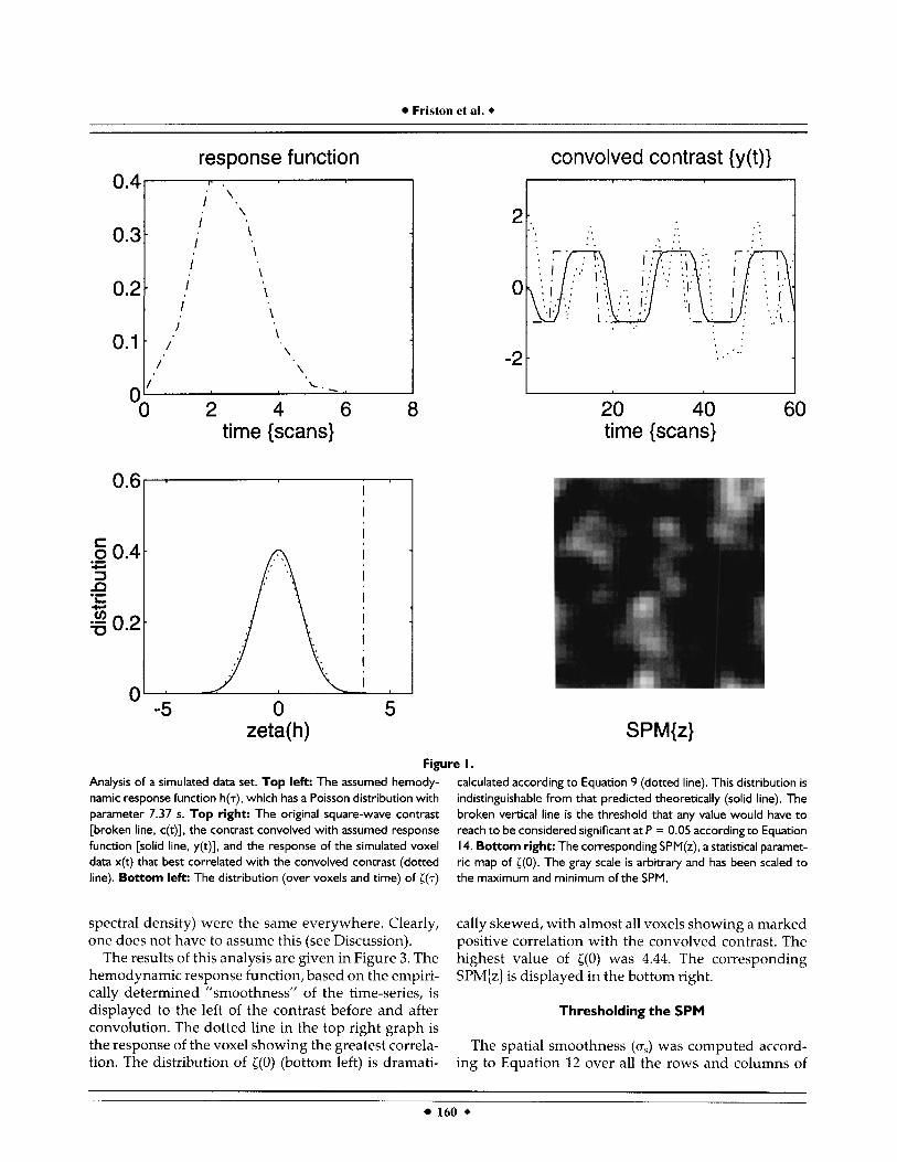
The results of this simulation are shown in Figure 1. The response function is shown (top left) with the resulting contrast before [c(t)] and after [y(t)] convolution with h(.) (top right). The agreement between the empirical and theoretical distributions of ((7) is clearly evident (lower left). The corresponding SPM{z] of {(O) is shown in the lower right. The highest value of ((0) obtained in this realization was 3.57. The time-series from the corresponding voxel is displayed with the contrasts (dotted line, top right). These high values (and apparent “following” of the contrast) can easily occur by chance and should not be overinterpreted in real data. No value exceeded the corrected threshold (broken vertical line, bottom left), which was 3.79 according to Equation 14 and the post hoc estimate of spatial smoothness (Equation 12). This estimated spatial smoothness (averaged over both dimensions) was 1.45 voxels and compares favorably with the expected value of 1.4 voxels.

ANALYSIS OF MRI TIME-SERIES

Data acquisition

The data used to illustrate the method were a time-series of 64 gradient-echo EPI single coronal slices (5 mm thick, 64 x 64 voxels) through the calcarine sulcus and extrastriate areas. Images were obtained every 3 s from a single subject using a 4.0-T whole body system, fitted with a small (27-cm diam- eter) z-gradient coil (TE 25 ms, acquisition time 41 ms). Photic stimulation (at 16 Hz) was provided by goggles fitted with light-emitting diodes. The stimulation was off for the first ten scans (30 s), on for the second ten, off for the third, and so on. Images were reconstructed without phase correction. The data were interpolated from 64 x 64 voxels to 128 x 128 voxels. Each voxel thus represented 1.25 x 1.25 x 5 mm of cerebral tissue.

Data preprocessing

Image manipulations and data analysis were performed in Matlab (Mathworks Inc., Sherborn, MD). The first four scans were removed to avoid magnetic saturation effects. The scans were corrected for (slight)

subject movement using nonlinear minimization and a computationally efficient cubic interpolation algorithm [Keys, 19811. Images were translated and rotated to minimize the sum of squares between each of the 64 images and their average (both scaled to the same mean intensity) using the Levenberg-Marquardt method [More, 19771. Only the 36 x 60 voxel subparti- tions (of the original images) containing the brain were subject to further analysis. All the time-series, for each voxel, were normalized to a mean of zero and convolved, in the time domain, with a Gaussian filter (full width at half maximum = 1.5 voxels) to suppress thermal noise.

Computing ((0)

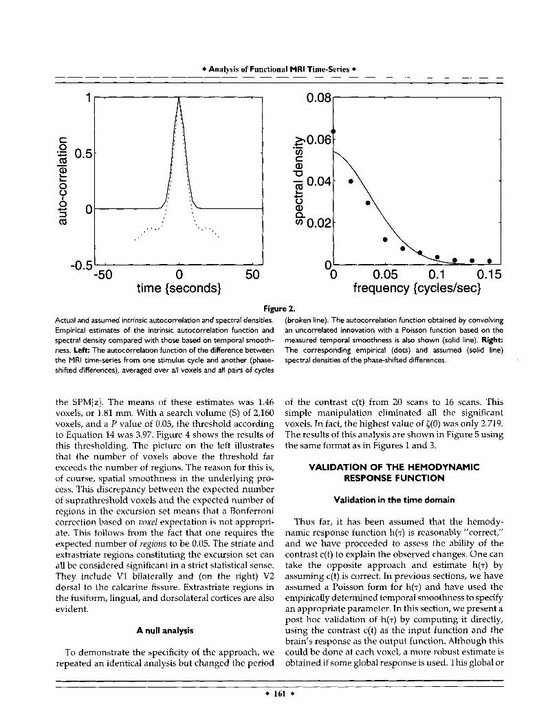
The real data were treated in an identical fashion to the simulated data. The temporal smoothness (a7) was estimated using Equation 12 to be 0.92, as mentioned above. This estimate was the mean over all intracere- bra1 voxels and corresponded to a value of 7.69 s for A, the parameter of our assumed Poisson response function h(7). To demonstrate that modeling intrinsic autocorrelations with a Gaussian form is reasonable, the empirical intrinsic autocorrelation functions and corresponding spectral density [gx(w)] are shown in Figure 2. These functions were obtained by averaging estimates over the differences between all pairs of 20 scan stimulation periods (phase-shifted differences). The data were windowed with a Hanning function before being subject to Fourier transform. The solid lines in Figure 2 correspond to the autocorrelations (and spectral density) that would be obtained by convolving an uncorrelated innovation with a Poisson function of parameter 7.69 s. The determination of the appropriate Poisson parameter does not require computation of either the autocorrelation function or spectral density, but uses the variance of the first derivatives as in Equation 12. These data are presented only to validate the Gaussian approximation

The contrast c(t) used in this example was, again, a square-wave that was positive during photic stimulation and negative otherwise. c(t) had zero-mean and unit variance. The measured correlation between y(t) and the MRI time-series x(t) was computed for all voxels and scaled by ,/u according to Equation 9 to produce ((0). Jv was 4.58, corresponding to 21 effective degrees of freedom. In other words, one accrues a “degree of freedom” every 2.85 scans. The reason v is the same for all voxels is that we assumed that the response function and intrinsic autocorrelations (and

for gx(0).

+ 159 +

Friston et al. +

0.4

0.3

0.2

0.1

n "0

0.6

c

3 P

.- o 0.4 c,

.- L c,

$0.2

response function I' . ' \ I .

I I

I

I

\

\

\

\

\ \ I

J \ \ /

/ \

2 4 time {scans}

I

-5 0

convolved contrast {y(t)}

-* t I . . . . .. . .

time {scans}

0 5 zeta(h) SPM{z)

Figure I. Analysis of a simulated data set. Top left: The assumed hemodynamic response function h($, which has a Poisson distribution with parameter 7.37 s. Top right: The original square-wave contrast [broken line, c(t)], the contrast convolved with assumed response function [solid line, y(t)], and the response of the simulated voxel data x(t) that best correlated with the convolved contrast (dotted line). Bottom left: The distribution (over voxels and time) of [ ( T )

calculated according to Equation 9 (dotted line). This distribution is indistinguishable from that predicted theoretically (solid line). The broken vertical line is the threshold that any value would have to reach to be considered significant at P = 0.05 according to Equation 14. Bottom right: The corresponding SPM(z), a statistical parametric map of ((0). The gray scale is arbitrary and has been scaled to the maximum and minimum of the SPM.

spectral density) were the same everywhere. Clearly, one does not have to assume this (see Discussion).

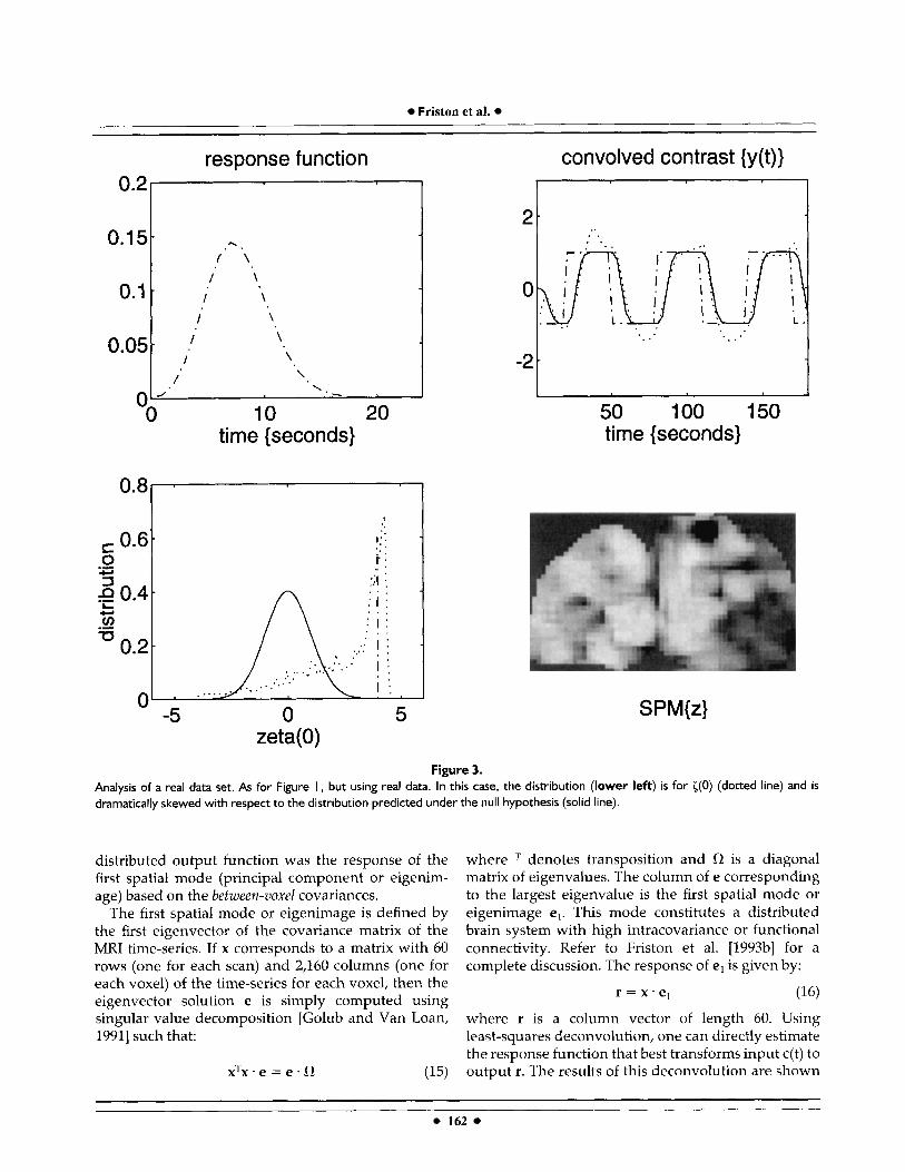
The results of this analysis are given in Figure 3. The hemodynamic response function, based on the empirically determined "smoothness" of the time-series, is displayed to the left of the contrast before and after convolution. The dotted line in the top right graph is the response of the voxel showing the greatest correlation. The distribution of ( (0) (bottom left) is dramati-

cally skewed, with almost all voxels showing a marked positive correlation with the convolved contrast. The highest value of i(0) was 4.44. The corresponding SPM{z] is displayed in the bottom right.

Thresholding the SPM

The spatial smoothness (a,) was computed according to Equation 12 over all the rows and columns of

160 +


time {seconds} frequency { c ycl es/sec} Figure 2.

Actual and assumed intrinsic autocorrelation and spectral densities. Empirical estimates of the intrinsic autocorrelation function and spectral density compared with those based on temporal smoothness. Left: The autocorrelation function of the difference between the MRI time-series from one stimulus cycle and another (phase- shifted differences), averaged over all voxels and all pairs of cycles

the SPM{z]. The means of these estimates was 1.46 voxels, or 1.81 mm. With a search volume (S) of 2,160 voxels, and a P value of 0.05, the threshold according to Equation 14 was 3.97. Figure 4 shows the results of this thresholding. The picture on the left illustrates that the number of voxels above the threshold far exceeds the number of regions. The reason for this is, of course, spatial smoothness in the underlying process. This discrepancy between the expected number of suprathreshold voxels and the expected number of regions in the excursion set means that a Bonferroni correction based on voxel expectation is not appropriate. This follows from the fact that one requires the expected number of regions to be 0.05. The striate and extrastriate regions constituting the excursion set can all be considered significant in a strict statistical sense. They include V1 bilaterally and (on the right) V2 dorsal to the calcarine fissure. Extrastriate regions in the fusiform, lingual, and dorsolateral cortices are also evident.

A null analysis

To demonstrate the specificity of the approach, we repeated an identical analysis but changed the period

(broken line). The autocorrelation function obtained by convolving an uncorrelated innovation with a Poisson function based on the measured temporal smoothness is also shown (solid line). Right: The corresponding empirical (dots) and assumed (solid line) spectral densities of the phase-shifted differences.

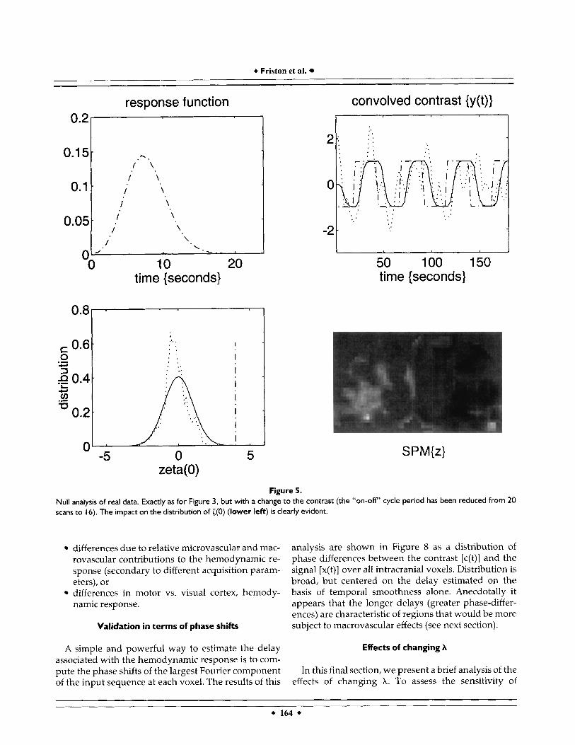
of the contrast c(t) from 20 scans to 16 scans. This simple manipulation eliminated all the significant voxels. In fact, the highest value of {(O) was only 2.719. The results of this analysis are shown in Figure 5 using the same format as in Figures 1 and 3.

VALIDATION OF THE HEMODYNAMIC RESPONSE FUNCTION

Validation in the time domain

Thus far, it has been assumed that the hemodynamic response function h(7) is reasonably “correct,” and we have proceeded to assess the ability of the contrast c(t) to explain the observed changes. One can take the opposite approach and estimate h(7) by assuming c(t) is correct. In previous sections, we have assumed a Poisson form for h(7) and have used the empirically determined temporal smoothness to specify an appropriate parameter. In this section, we present a post hoc validation of h(7) by computing it directly, using the contrast c(t) as the input function and the brain’s response as the output function. Although this could be done at each voxel, a more robust estimate is obtained if some global response is used. This global or

Friston et al.

response function convolved contrast (y(t)}

o.05i / ,__I \ /

'.-

10 20 0' 0

time {seconds}

0.8

C 0.6 0 S .- w

g 0.4

0.2 e L +-' cn

-5 0 5 0, ' .

50 100 150 time (seconds}

SPM{z} zeta(0)

Figure 3. Analysis of a real data set. As for Figure I, but using real data. In this case, the distribution (lower left) is for ((0) (dotted line) and is dramatically skewed with respect to the distribution predicted under the iiull hypothesis (solid line).

distributed output function was the response of the first spatial mode (principal component or eigenimage) based on the between-voxel covariances.

The first spatial mode or eigenimage is defined by the first eigenvector of the covariance matrix of the MRI time-series. If x corresponds to a matrix with 60 rows (one for each scan) and 2,160 columns (one for each voxel) of the time-series for each voxel, then the eigenvector solution e is simply computed using singular value decomposition [Golub and Van Loan, 19911 such that:

xTx .e = e . R (15)

where denotes transposition and R is a diagonal matrix of eigenvalues. The column of e corresponding to the largest eigenvalue is the first spatial mode or eigenimage el. This mode constitutes a distributed brain system with high intracovariance or functional connectivity. Refer to Friston et al. [1993b] for a complete discussion. The response of el is given by:

r = x ' e , (16) where r is a column vector of length 60. Using least-squares deconvolution, one can directly estimate the response function that best transforms input c(t) to output r. The results of this deconvolution are shown

162


signficiant covariances

Figure 4. Thresholding the SPM[z]. Left: The SPM(z) from Figure 3 is presented as a surface rendering, with the corrected threshold (corrected for multiple nonindependent comparisons according to Equation 14). Right: The resulting “excursion set” is highlighted and includes V I and several extrastriate regions according to the atlas of Talairach and Tournoux [ 19881.

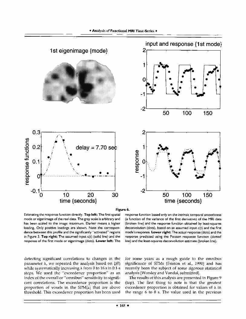
in Figure 6, where the ”memory” of the convolution has been restricted to ten scans. The first eigenimage or mode (top left) reveals high loadings in the same areas identified by the more conventional (hypothesis- led) analysis of the previous sections. The corresponding response is shown with the contrast (top right). The results of the least-squares deconvolution (dots) agree remarkably with the hemodynamic response function based only on the temporal autocorrelations (broken line). The predicted and actual responses of the first mode are compared in the lower right. The predicted time courses are simply the contrast convolved with h(7) (broken line) and the empirically determined response function (solid line). It is apparent that the empirical response function has a slightly more protracted tail, with some hint of biphasic structure. One might conjecture that this feature may reflect macrovascular effects as remote regions are drained.

Validation in the frequency domain

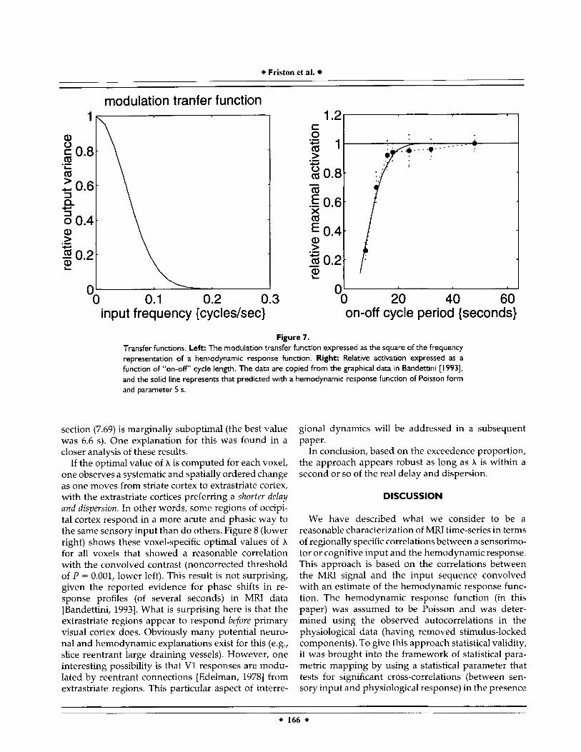
The hemodynamic response function “behaves es- sentially as a low-pass filter in the detection of neuronal firing” [Bandettini, 19931. In other words, higher- frequency inputs are more severely attenuated than low-frequency inputs. The dependency of output variance on input frequency is captured by the (squared) transfer function 1H(w) I seen in Figure 7

(left). This example is for a Poisson parameter of 5 s and demonstrates the downwards modulation of output variance with increasing frequency of a periodic input. For example, the variance of a periodic input at 0.1 cycles/s (a stimulus cycle length of 10 s) is attenuated to about 20 percent. The hemodynamic response function can provide quite a powerful prediction of the brain’s capacity to follow a periodic stimulus when presented at increasing frequencies. Bandettini et al. have examined this phenomenon using fast, self- paced, sequential finger-thumb opposition at different on-off switching frequencies, ranging from period lengths of 50 s (e.g./ 25 s of finger opposition and 25 at rest) to 2 s. The data reported in Bandettini [1993] are in terms of relative activation or amplitude of response. These data are in excellent agreement with theoretical predictions based on a Poisson hemodynamic response function (Fig. 7, left). The theoretical values were derived by simply convolving a square- wave contrast of appropriate frequency with a Pois- son response function (parameter 5 s) and taking the maximum amplitude difference. The Poisson parameter used here (5 s) is smaller than that calculated on the basis of our photic stimulation data and may reflect a number of differences, including:

differences in the neuronal response to varying task conditions

+ Friston et al.

0.2

0.1 5

0.1

0.05-

-

2 - . A .

- i \

( \

I \

I \

0

\

-2 1 .’ \ \

- . ‘. /

n.’

0.8

c 0.6 0 3 .- +

L 0.4- + a m .- 0.2

0-

50 100 150 time {seconds}

... , I

I I I 1 I

I I

a , , . . . . .. . *.

-

. .

-

‘

SPM{z}

Figure 5. Null analysis of real data. Exactly as for Figure 3, but with a change to the contrast (the “on-off’ cycle period has been reduced from 20 scans to 16). The impact on the distribution of ((0) (lower left) is clearly evident.

differences due to relative microvascular and macrovascular contributions to the hemodynamic response (secondary to different acquisition parameters), or differences in motor vs. visual cortex, hemodynamic response.

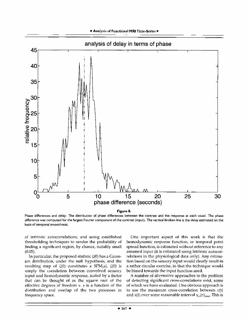
analysis are shown in Figure 8 as a distribution of phase differences between the contrast [c(t)J and the signal [x(t)] over all intracranial voxels. Distribution is broad, but centered on the delay estimated on the basis of temporal smoothness alone. Anecdotally it appears that the longer delays (greater phase-differences) are characteristic of regions that would be more subject to macrovascular effects (see next section). Validation in terms of phase shifts

A simple and powerful way to estimate the delay associated with the hemodynamic response is to compute the phase shifts of the largest Fourier component of the input sequence at each voxel. The results of this

Effects of changing h

In this final section, we present a brief analysis of the effects of changing X. To assess the sensitivity of

+ 164 +


1 -

0 -

-1

0.2

’= 0.2

Q) 0.1

v) c 0 0 c S

v) c

+

% . -* 0 . . e.5 . . . . . . . . . + .

” 0 0 . . .p -! -

0 v)

2

1 st eigenimage {mode}

/. \ i ’ t

I ’\. delay = 7.70 se

.I‘ \ \. . I

I \ . / \

‘. . . r------ . . . . . . . . . . . . . . . . . . . . . *..-..

Estimating the response function directly. Top left: The first spatial mode or eigenimage of the real data. The gray scale is arbitrary and has been scaled to the image maximum. Darker means a higher loading. Only positive loadings are shown. Note the correspon- dence between this profile and the significantly “activated” regions in Figure 3. Top right: The assumed input c(t) (solid line) and the response of the first mode or eigenimage (dots). Lower left: The

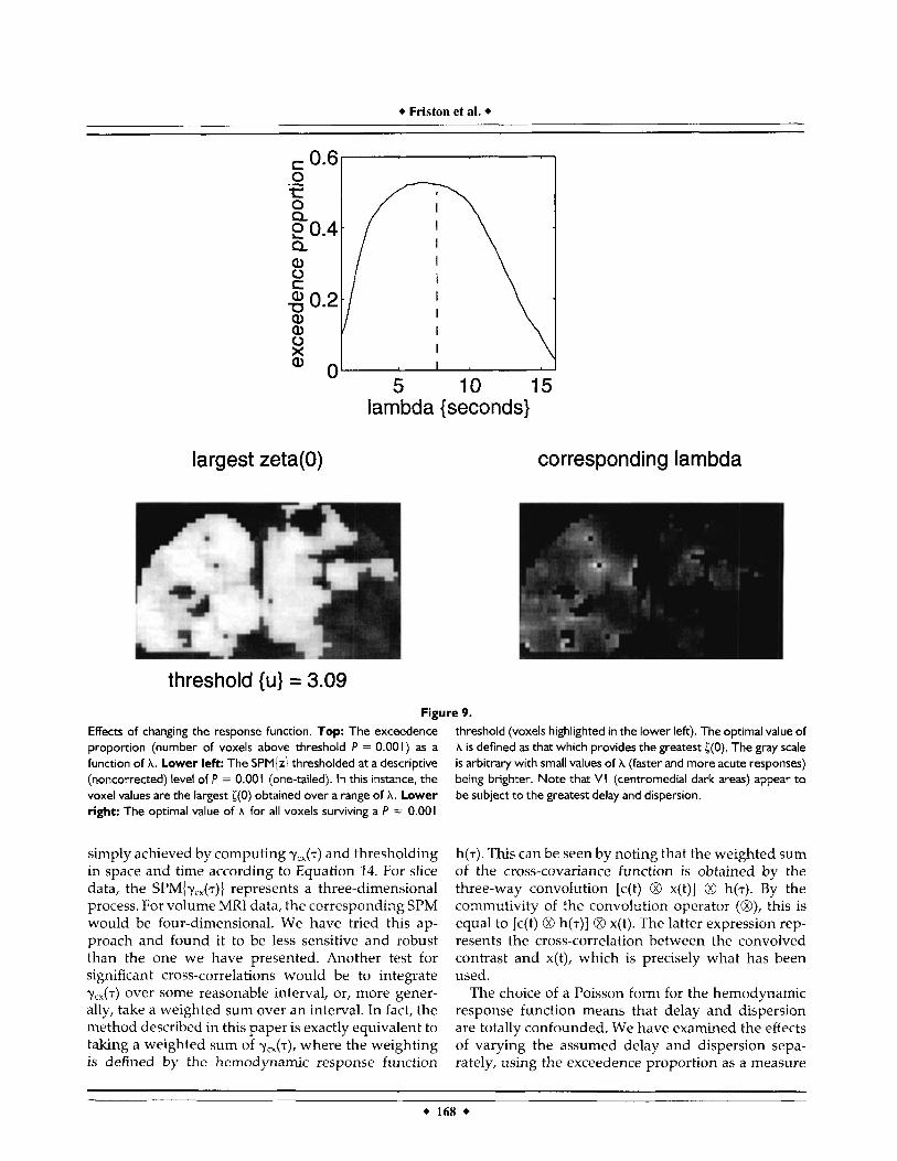
detecting significant correlations to changes in the parameter A, we repeated the analysis based on {(O) while systematically increasing A from 0 to 16 s in 0.1-s steps. We used the “exceedence proportion” as an index of the overall or ”omnibus” sensitivity to significant correlations. The exceedence proportion is the proportion of voxels in the SPM{z} that are above threshold. This exceedence proportion has been used

input and response (1st mode}

21---1

-21 50 100 150

-2’ I 50 100 150 time (seconds}

0 10 20 30 time {seconds}

-0.1 ‘ Figure 6.

+ 165

response function based only on the intrinsic temporal smoothness (a function of the variance of the first derivative) of the MRI data (broken line) and the response function obtained by least-squares deconvolution (dots), based on an assumed input c(t) and the first mode’s response. Lower right: The actual response (dots) and the response predicted using the Poisson response function (dotted line) and the least-squares deconvolution estimate (broken line).

for some years as a rough guide to the omnibus significance of SPMs [Friston et a]., 19901 and has recently been the subject of some rigorous statistical analysis [Worsley and Vandal, submitted].

The results of this analysis are presented in Figure 9 (top). The first thing to note is that the greatest exceedence proportion is obtained for values of A in the range 6 to 8 s. The value used in the previous

6 Friston et al.

modulation tranfer function 1.21 1

-0 input frequency { cycles/sec} on-off cycle period {seconds}

Figure 7. Transfer functions. Left: The modulation transfer function expressed as the square of the frequency representation of a hernodynamic response function. Right: Relative activation expressed as a function of “on-off’ cycle length. The data are copied from the graphical data in Bandettini [ 19931, and the solid line represents that predicted with a hernodynamic response function of Poisson form and parameter 5 s.

section (7.69) is marginally suboptimal (the best value was 6.6 s). One explanation for this was found in a closer analysis of these results.

If the optimal value of A is computed for each voxel, one observes a systematic and spatially ordered change as one moves from striate cortex to extrastriate cortex, with the extrastriate cortices preferring a shorter delay and dispersion. In other words, some regions of occipi- tal cortex respond in a more acute and phasic way to the same sensory input than do others. Figure 8 (lower right) shows these voxel-specific optimal values of A for all voxels that showed a reasonable correlation with the convolved contrast (noncorrected threshold of P = 0.001, lower left). This result is not surprising, given the reported evidence for phase shifts in response profiles (of several seconds) in MRI data [Bandettini, 19931. What is surprising here is that the extrastriate regions appear to respond before primary visual cortex does. Obviously many potential neuronal and hemodynamic explanations exist for this (e.g., slice reentrant large draining vessels). However, one interesting possibility is that V1 responses are modu- lated by reentrant connections [Edelman, 19781 from extrastriate regions. This particular aspect of interre-

gional dynamics will be addressed in a subsequent paper.

In conclusion, based on the exceedence proportion, the approach appears robust as long as A is within a second or so of the real delay and dispersion.

DISCUSSION

We have described what we consider to be a reasonable characterization of MRI time-series in terms of regionally specific correlations between a sensorimotor or cognitive input and the hemodynamic response. This approach is based on the correlations between the MRI signal and the input sequence convolved with an estimate of the hemodynamic response function. The hemodynamic response function (in this paper) was assumed to be Poisson and was determined using the observed autocorrelations in the physiological data (having removed stimulus-locked components). To give this approach statistical validity, it was brought into the framework of statistical parametric mapping by using a statistical parameter that tests for significant cross-correlations (between sensory input and physiological response) in the presence


analysis of delay in terms of phase 45 I I I I I I

I 1 I

I I

I

I I I I I 1

40

35

30

-

-

- r 0 c a u 25- 2 .- > 20-

15-

10-

5-

Y-

a ca Q)

w

+

I I I

I I I

I

I I n. I I

I \

-0 5 10 15 20 25 30 phase difference (seconds)

Figure 8. Phase differences and delay. The distribution of phase differences between the contrast and the response at each voxel. The phase difference was computed for the largest Fourier component of the contrast (input). The vertical broken line is the delay estimated on the basis of temporal smoothness.

of intrinsic autocorrelations; and using established thresholding techniques to render the probability of finding a significant region, by dhance, suitably small (0.05).

In particular, the proposed statistic ((0) has a Gauss- ian distribution, under the null hypothesis, and the resulting map of <(O) constitutes a SPM{z). c(O) is simply the correlation between convolved sensory input and hemodynamic response, scaled by a factor that can be thought of as the square root of the effective degrees of freedom w. w is a function of the distribution and overlap of the two processes in frequency space.

One important aspect of this work is that the hemodynamic response function, or temporal point spread function, is estimated without reference to any assumed input (it is estimated using intrinsic autocorrelations in the physiological data only). Any estimation based on the sensory input would clearly result in a rather circular exercise, in that the technique would be biased towards the input function used.

A number of alternative approaches to the problem of detecting significant cross-correlations exist, some of which we have evaluated. One obvious approach is to use the maximum cross-correlation between c(t) and x(t) over some reasonable interval Y J T ) , , , ~ ~ . This is

167

+ Friston et al. +

0.6 0 I= 0 Q

Q a, 0 c

a, Q) 0 X

.-

9 0.4

$0.2

a n

I a rg es t zeta (0)

5 10 15 U

lambda (seconds}

threshold {u} = 3.09 Figure 9.

Effects of changing the response function. Top: The exceedence proportion (number of voxels above threshold P = 0.001) as a function of A. Lower left The SPM(z) thresholded at a descriptive (noncorrected) level of P = 0.001 (one-tailed). In this instance, the voxel values are the largest ((0) obtained over a range of A. Lower right: The optimal value of A for all voxels surviving a P = 0.001

simply achieved by computing y,,(~) and thresholding in space and time according to Equation 14. For slice data, the SPM{y,,(7)) represents a three-dimensional process. For volume MRI data, the corresponding SPM would be four-dimensional. We have tried this approach and found it to be less sensitive and robust than the one we have presented. Another test for significant cross-correlations would be to integrate y,,(~) over some reasonable interval, or, more gener- ally, take a weighted sum over an interval. In fact, the method described in this paper is exactly equivalent to taking a weighted sum of ycx(7), where the weighting is defined by the hemodynamic response function

corresponding lambda

threshold (voxels highlighted in the lower left). The optimal value of A is defined as that which provides the greatest ((0). The gray scale is arbitrary with small values of A (faster and more acute responses) being brighter. Note that VI (centrornedial dark areas) appear to be subject to the greatest delay and dispersion.

h(7). This can be seen by noting that the weighted sum of the cros~-covariance function is obtained by the three-way convolution [c(t) O x(t)] 0 h(7). By the commutivity of the convolution operator (O), this is equal to [c(t) O h ( ~ ) ] 0 x(t). The latter expression represents the cross-correlation between the convolved contrast and x(t), which is precisely what has been used.

The choice of a Poisson form for the hemodynamic response function means that delay and dispersion are totally confounded. We have examined the effects of varying the assumed delay and dispersion sepa- rately, using the exceedence proportion as a measure

+ 168 +


of omnibus sensitivity. In these analyses, we used the y-distribution, which has two parameters and allows the independent manipulation of mean and variance. We did not report the results of this analysis because they did not contribute any significant insight. In general, the exceedence proportion showed exactly the same dependence on delay as for the Poisson form. The dependence on dispersion was much less marked. We could have used a Gaussian response function and set the delay equal to dispersion (for large values of A, this and the Poisson function are the same). The aesthetic advantage of the Poisson function is that it only exists for positive lag (7).

Obviously, there are many variants on the details we have presented here. The central tenets of the approach are:

Regonal specific associations are assessed between neuronal activity and a stimulus or task parameter in terms of correlations. The appropriate correlation is between the observed hemodynamic response and the hypoth- esized input, which has been convolved with a response function. The response function is specified without reference to an assumed input. Care is taken to ensure that, in the absence of any response, intrinsic temporal and spatial autocorrelations do not subtend spurious correlations (i.e., the experiment-wise false-positive rate is main- tained at a suitably low level).

Within these constraints, a number of variants deserve mention. First, in the analysis above, it was assumed that the response function and intrinsic autocorrelations were the same for all voxels. An identical analysis performed in parallel for each voxel would allow for regional variation in the response function. Our analyses (see last section) suggest that these regional variations can be substantial. This extension would certainly increase sensitivity, but would require long time-series, to ensure robust estimates of the intrinsic spectral density gx(o). A second variant would involve estimating the response function on the basis of independent data; for example, a second study or dividing the same study into two sections and using the SVD or PCA approach and least-squares deconvolution (Haxby J, personal communication).

Although we used temporal smoothness to estimate both the intrinsic spectral density of the MRI signal and the response function, it is important to note that the first application is mandatory; the second is not. Any response function will, under the null hypothesis, render the distribution of {(O) Gaussian. Despite the fact that sensitivity to real change will be optimized

when the dispersion or variance of the response function "matches" the intrinsic autocorrelations, no statistical requirement exists for this matching to be implemented. In other words, the response function is a personal choice. Complicated biphasic response functions are attractive in the sense that they are capable of modeling the "undershoot" effect. How- ever, the data did not suggest that this extension was justified in the examples above.

One particular constraint imposed by a Poisson form is that delay and dispersion are yoked. This may be inappropriate for some data, and this constraint should not be considered a cornerstone of the proposed method. One particular fallacy of linkmg the delay and dispersion is revealed when considering the effect of temporal smoothing of the data to increase signal to noise. Here, the underlying response function will be subject to this smoothing; and its effective dispersion will increase. This would be correctly de- tected and modeled by post hoc estimates of smoothness. However, the "correct" delay will not have changed. In some instances, it may be best to fix the response function to some appropriate delay and allow its variance to be dictated by uf (e.g., using the y-distribution).

In the method presented, the impact of thermal noise was suppressed by temporal smoothing at a data preprocessing stage. With longer time-series, it may be possible to adopt a more formal approach by segregat- ing the data into an uncorrelated white (or Raleigh) noise and a physiological autocorrelated process. Many linear devices exist for this sort of analysis (e.g., autoregressive and moving average models). How- ever, they are usually not considered in the context of very short time-series.

Correlations or categories?

The principle of correlating sensorial or behavioral parameters with cerebral excitation has a long history in neuroscience, from the days of Goltz and Ferrier [ e g , Ferrier, 1875; Goltz, 1881; Phillips et al., 19841 to modern-day approaches that use exogenous stimulation, e.g., magneto-simulation or endogenous activity (PET and MRI). Correlations in microelectrode record- ing and functional imaging data have received special attention recently, as they are a possible index of functional and effective connectivity [Gerstein and Perkel, 1969; Friston et al., 1993133.

Although a fundamental equivalence exists between testing for specific time-dependent changes with contrasts in analysis of (co-)variance of PET data and correlating a time-dependent parameter with

+ 169 +

+ Friston et al. +

MRI data (refer to Friston et al. [1993a] for a concrete illustration of this point), it is important to acknowl- edge the differences: MRI data represent time-series that lend themselves directly to signal processing. For example, in this paper, using a few standard results from the theory of stochastic processes, one can solve the problem of detecting cross-correlations in the presence of autocorrelations and avoid what could have been a discursive and dense statistical analysis.

This paper has focused exclusively on correlations for detecting significant activations. An alternative, found in the recent functional MRI literature, is to categorize the MRI time-series into activation and baseline scans and express the mean difference in some form. Researchers have had profound reservations about this approach related to the observation that the residual MRI signal around the mean for each stimulus-cycle is not normally distributed [Baker J, personal communication]. The analysis presented in this paper concurs with these reservations. Although the residual variability about the convolved contrast y(t) is normally distributed, the probability that it will be similarly distributed about a horizontal line run- ning from stimulus onset to offset is low. The MRI time-series reflects a true dynamic response to an input, characterized by its response function. To pre- tend that this response following stimulus onset constitutes a single category is not really tenable. The proper way to categorize these time-series conceptu- ally is in terms of offset from stimulus onset. For example, the set of first scans after stimulus onset is a different category from the set of second scans following stimulus onset. The residuals about the means of these categories will be normally distributed. The convolved contrast implicitly assumes the latter form of categorization because only these scans have the same values of y(t).

Implicit in phase-shifting (as a tool to estimate intrinsic autocorrelations) is the requirement that stimulus cycles are continuously repeated. A fundamental point to be made here is: If implementation of intrasubject signal averaging in its broadest sense is the goal, then multiple presentations of the same stimulus-cycle are obligatory (the more the better). This places significant constraints on experimental design. The key theme, again, is that the object that is averaged is a complete stimulus-cycle, not repeated scans within a cycle. A failure to recognize this will sacrifice all the rich nonlinear information about an evoked neuronal and hemodynamic transient for the apparent ease of simple categorical comparisons. Ironically, this non-

linearity invalidates a parametric approach to averaging scans from the same stimulus-cycle (see above).

In the context of MRI data, correlational approaches offer many advantages over alternative approaches. One key issue is that the correlation between sensory input and hemodynamics will not be sensitive to any artifact that is orthogonal (independent) to the input. These artifacts include movement artifacts and low- frequency aliasing artifacts due to an interaction between the repeat time and cardiac, respiratory, and heart rate variability cycles. The proposed approach has the following interesting feature regarding movement artifacts. Because the effect of movement on signal is not subject to delay or dispersion (whereas the effect of evoked neuronal activity is), convolving the contrast with a hemodynamic response function will render the correlations insensitive to movement associated with changing stimuli or tasks.

In conclusion, we hope to have presented some reasonable solutions to a relatively simple problem- how to identify regionally specific correlations between sensory, cognitive, or behavioral parameters and cerebral physiology measured with functional MRI.

ACKNOWLEDGMENTS

We wish to thank Jack Belliveau, John Baker, Jim Haxby, and Nick Lange for helpful discussions about these issues. The work by K.J.F. was performed as part of the Institute Fellows in Theoretical Neurobiology research program at The Neurosciences Institute, which is supported by the Neurosciences Research Foundation. The Foundation receives major support for this research from the J.D. and C.T. MacArthur Foundation and the Lucille P. Markey Charitable Trust. K.J.F. was a W.M. Keck Foundation Fellow.

REFERENCES

Adler RJ, Hasofer AM (1981): The Geometry of Random Fields. New York: John Wiley & Sons.

Aertsen A, Preissl H (1991): Dynamics of activity and connectivity in physiological neuronal networks. In: Schuster HG (ed): Non Linear Dynamics and Neuronal Networks. New York: VCIH Publishers, pp 281-302.

Bandettini PA (1993): MRI studies of brain activation: Temporal characteristics. In: Functional MRI of the Brain. Berkely: Society of Magnetic Resonance in Medicine, California, p 143-151.

Bandettini PA, Wong EC, Hinks RS, Tikofsky RS, Hyde JS (1992): Time course EPI of human brain function during task activation. Magn Reson Med 25:390-397.

Bandettini PA, Jesmanowicz A, Wong EC, Hyde JS (1993) Processing strategies for time course data sets in functional MRI of the human brain. Magn Reson Med 30:161-173.

- + 170 +


Cox DR, Miller HD (1980): The theory of stochastic processes. New York: Chapman and Hall.

Edelman GM (1978): Group selection and phasic reentrant signal- ing: A theory of higher brain function. In: Edelman GM, Mountcastle VB (eds): The Mindful Brain. Cambridge: MIT Press, pp 55-100.

Ferrier D (1875): Experiments on the brain of monkeys. Proc R SOC Lond, 23:409-430.

Fox PT, Raichle ME, Mintum MA, Dence C (1988): Nonoxidative glucose consumption during focal physiologic neural activity. Science 24 1 : 462.

Friston KJ, Frith CD, Liddle PF, Dolan RJ, Lammertsma AA, Frackowiak RSJ (1990): The relationship between global and local changes in PET scans. J Cereb Blood Flow Metab 10:458- 466.

Friston KJ, Frith CD, Liddle PF, Frackowiak RSJ (1991): Comparing functional (PET) images: The assessment of significant change. J Cereb Blood Flow Metab 11690-699.

Friston KJ, Jezzard P, Frackowiak RSJ, Turner R (1993a): Characteriz- ing focal and distributed physiological changes with MRI and PET. In: Functional MRI of the Brain-Syllabus. Berkely: Society of Magnetic Resonance in Medicine, California, pp 207-216.

Friston KJ, Frith CD, Liddle PF, Frackowiak RSJ (1993b): Functional connectivity: The principal component analysis of large (PET) data sets. J Cereb Blood Flow Metab 13:5-14.

Friston KJ, Worsley KJ, Frackowiak RSJ, Mazziotta JC, Evans AC (in press): Assessing the significance of focal activations using their spatial extent. Human Brain Mapping.

Frostig RD, Lieke RR, Ts’o DY, Grindvald A (1990): Cortical functional architecture and local coupling between neuronal activity and the microcirculation revealed by in vivo high resolution optical imaging of intrinsic signals. Proc Natl Acad Sci USA

Gerstein GL, Perkel DH (1969): Simultaneously recorded trains of action potentials: Analysis and functional interpretation. Science 164: 828-830,

876082-6086.

Goltz F (1881): In: MacCormac W (ed): Transactions of the 7th International Medical Congress, Vol. 1. London: Kolkmann, pp 218-228.

Golub GH, Van Loan CF (1991): Matrix computations, 2nd ed. Baltimore: The Johns Hopkins University Press, pp 241-248.

Grimmett G, Welsh D (1986): Probability and Introduction. Oxford: Clarendon Press.

Hasofer AM (1978): Upcrossings of random fields. Suppl Adv Appl Prob 10:1421.

Keys RG (1981): Cubic convolution interpolation for digital image processing. IEEE Trans Acoust Speech Signal Process 29:1153- 1160.

Kwong KK, Belliveau JW, Cheder DA, Goldberg IE, Weisskoff RM, Poncelet BP, Kennedy DN, Hoppel BE, Cohen MS, Turner R, Cheng HM, Brady TJ, Rosen BR (1992): Dynamic magnetic resonance imaging of human brain activity during primary sensory stimulation. Proc Natl Acad Sci USA 89:5675-5679.

More JJ (1977): The Levenberg-Marquardt algorithm: Implementa- tion and Theory. In: Watson GA (ed): Numerical Analysis. Lecture Notes in Mathematics 630. Berlin: Springer-Verlag, pp 105-116.

Nelson JI, Salin PA, Munk MHJ, Arzi M, Bullier J (1992): Spatial and temporal coherence in cortico-cortical connections: A cross- correlation study in areas 17 and 18 in the cat. Visual Neurosci 9:21-37.

Ogawa S, Tank DW, Menon R, Ellermann JM, Kim SG, Merkle H, Ugurbil K (1992): Intrinsic signal changes accompanying sensory stimulation: Functional brain mapping with magnetic resonance imaging. Proc Natl Acad Sci USA 89:5951-5955.

Phillips CG, Zeki S, Barlow HB (1984): Localization of function in the cerebral cortex: Past, present and future. Brain 107:327-361.

Talairach P, Tournoux J (1988): A Stereotactic Coplanar Atlas of the Human Brain. Stuttgart: Thieme.

Worsley KJ, Vandal (submitted): Tests for changes in random fields with applications to medical images.

Worsley KJ, Evans AC, Marrett S, Neelin P (1992): A three- dimensional statistical analysis for rCBF activation studies in human brain. J Cereb Blood Flow Metab 12:900-918.

+ 171 +

Analysis of Functional MRI Time-Serieskarl/Analysis of functional MRI time-series.pdf · + Human...

Documents

Transcript of Analysis of Functional MRI Time-Serieskarl/Analysis of functional MRI time-series.pdf · + Human...