Analysis of flows and prediction of CH10 airfoil for ...

Advances in Aircraft and Spacecraft Science, Vol. 8, No. 2 (2021) 87-109

DOI: https://doi.org/10.12989/aas.2021.8.2.087 87

Copyright © 2021 Techno-Press, Ltd.

http://www.techno-press.org/?journal=aas&subpage=7 ISSN: 2287-528X (Print), 2287-5271 (Online)

Analysis of flows and prediction of CH10 airfoil for unmanned arial vehicle wing design

Abdul Aabid1,2, Liyana Nabilah Binti Khairulaman2a and Sher Afghan Khan2b

1Department of Engineering Management, College of Engineering, Prince Sultan University, P.O. Box 66833, Riyadh 11586, Saudi Arabia

2Department of Mechanical Engineering, Faculty of Engineering, International Islamic University Malaysia, 53100, Kuala Lumpur, Malaysia

(Received March 28, 2020, Revised November 27, 2020, Accepted December 2, 2020)

Abstract. The unmanned aerial vehicle (UAV) is becoming popular from last two decades and it has been utilizing in enormous applications such as aerial monitoring, military purposes, rescue missions, etc. Hence, the present work focused on the design of the UAV wing considering the CH10 airfoil. In this paper, the computational fluid dynamic analysis on CH10 cambered airfoil has been conducted to achieve the preliminary results on the aerodynamic lift and drag coefficients. The airfoil has a chord length of 1 meter and has been subjected to low Reynolds numbers of 500 000, which is the standard operating Reynolds number for UAV wing design. The C-type fluid domain has been constructed at 30C upstream and downstream of the airfoil to initialize the boundary conditions. The angle of attack ranging from 0° to 14° with the increment of 2° has been done by changing the direction of the freestream velocity. The aerodynamic characteristics have been numerically computed using Spallart-Allmaras and Transient SST models. The aerodynamic coefficients achieved by these two models have been validated based on the XFOIL data. The contours of static pressure and velocity magnitude at 0°, 5°, 10°, and 12°

angle of attack have been portrayed. The static pressure distribution around the airfoil has been visually observed to analyze its influence on the aerodynamic coefficients. The velocity magnitude relation to the static pressure distribution has been approved based on Bernoulli’s equation such that increasing velocity magnitude has decreased the static pressure. The present results show that the Transient SST model has shown better flow prediction for an airfoil subjected to low Reynolds number flow.

Keywords: airfoil; CH10; NACA 2412; CFD simulation; aerodynamics, UAV; FVM; ANSYS

1. Introduction

The growing interest in designing a high performance unmanned aerial vehicle (UAV) has

triggered a debate on which type of airfoil should be used to meet the mission expectations. The

high lift with low operating Reynolds number airfoils is the most preferred; however, with various

choices and selections, it has been almost inconclusive to select one airfoil that could fit into the

Corresponding author, Ph.D., Post-Doctoral Fellow, E-mail: [email protected],

[email protected] aGraduate Student, E-mail: [email protected] bPh.D., Professor, E-mail : [email protected]

Abdul Aabid, Liyana Nabilah Binti Khairulaman and Sher Afghan Khan

Fig. 1 CH10 airfoil plot (Khan et al. 2018)

problem. The only parameter that can be used to make the decision is based on the UAV

application itself. One of the successful experiments that have been conducted in 2018 is

emphasized the humanitarian application (Khan et al. 2018). Where the remote-controlled UAV is

used to drop 1.36078 kg (3-lb) of payload at an altitude of 30.48 m (100 ft) above the ground

without compromising the stability. The cambered CH10 (smoothed) airfoil (Fig. 1) has been used

in this study to construct the wing structure for the UAV. The nobility of the experiment has given

an idea to investigate the fluid dynamics of the airfoil.

The cambered CH10 airfoil has been analysed based on the flow field and pressure distribution

over the airfoil surfaces to deduct the lift coefficient, drag coefficient, and velocity magnitude. The

previous works related to CH10 airfoil has been reviewed to strengthen the fundamental

knowledge of its nature and to be determined as references for the methodology. The

computational fluid dynamics (CFD) has been used to compute these airfoil properties by applying

mathematical modelling and numerical simulation through the finite volume method (FVM). The

FVM will be conducted by using ANSYS Fluent software to simulate the fluid dynamics around

the airfoil. Finally, the results from simulation have been discussed to be analysed and

benchmarked based on the present work. The critical comments on the results will be made in the

discussions to improve the understanding of fluid dynamics.

The objective of this paper, the modelling of the cambered CH10 airfoil is done in ANSYS

Fluent with the assumption such that the free stream velocity, V∞ passed through the two-

dimensional (2D) shape of the airfoil. The boundary conditions of the fluid domain are set such

that the flow at the front of the airfoil is called upstream (or ‘inlet’) flow, and the flow after the

airfoil is called downstream (or ‘outlet’) flow. The upper line of the geometry is set as the ‘top

wall,’ and the lower edge of the geometry is set as the ‘bottom wall.’ The mesh that is constructed

must be a structural, Quadrilateral mesh. Since the perimeter of the airfoil is a high-stress area,

thus, the mesh generated should be high as well. Validation of present CFD results by selecting the

NACA 2412 airfoil due to the availability of experimental data. To obtain the preliminary results

an aerodynamic lift and drag coefficient, pressure distribution, and velocity magnitude of CH10

airfoil was considered.

2. Literature review

The literature survey has been classified based on CFD work, Reynolds number, and UAV’s,

which are closely related to the present problem. Other few studies also highlighted which gives an

idea of the investigation of the present work.

The CFD is a well-known predictive tool providing a cost-effective simulation of physical

phenomena (Rizvi 2017) and heat transfer (Sagat et al. 2012). The physical aspects of the fluid

flow around the airfoil, such as shock waves, slip surfaces, boundary layers, and turbulence of an

88


airfoil, can be understandable with the aid of CFD simulation. It simplifies the liquid or gas flow

problem around/within a specified model by solving the governing equations. The governing

equations are the conservation of mass, momentum, and energy (Lomax et al. 2013) by using the

discretization method through the grid or mesh generation process. Besides being a cost-effective

method to solve the formulated engineering problems, CFD also gains its reputation for accuracy

as it could achieve a close agreement to the experimental results (Kandwal and Singh 2012). These

physical phenomena will be simulated based on the numerical methods of modified partial

differential equations. CFD simulation is widely used in the aerospace study as it has it could

predict the surface pressures, skin friction, lift and drag at the angle of attack below stall with high

accuracy. Besides, CFD simulation is much preferable compared to the experimental method due

to the high cost of the experimental setup and the time-constraint. Therefore, the results obtained

will be much faster and accurate compared to a series of lab tests.

On the other hand, the range of low Reynolds number is identified between 104 and 106

(Lissaman 1983). From 102 to 104 is the range of Reynolds number for the insects and small model

airplanes where the characteristics of the laminar flow are described. The airfoil performance

within this range is relatively low but gradually increases with increasing Reynolds number. From

105 to 106 is the range for the sizeable radio-controlled model aircraft, foot-launched ultralight,

man-carrying hanggliders, and the human-powered aircraft (Carmichael 2018). The UAV’s wing

is often designed to be operated between this range of Reynolds number to obtain a high lift-to-

drag ratio. Therefore, a high-lift low Reynolds number is best chosen to achieve the objective. A

high lift coefficient is desirably required to reduce the size of the lifting surface. However, at a

lower Reynolds number, the airfoil is affected mainly by the viscosity that causes high drag, thus,

limiting the airfoil from achieving a high lift coefficient. Therefore, increasing the Reynolds

number is necessary to improve airfoil effectiveness. The performance transition usually takes

place at a critical Reynolds number of 70 000, where drastic improvement of smooth airfoil

performance is vividly observed in Fig. 2. The performance transition of the smooth airfoil takes

place within the range of Reynolds number between 105 to 106 as there is a sudden increment of

maximum lift-to-drag ratio. Compared to a rough or turbulent airfoil, the airfoil performance is

increased only slightly with increasing Reynolds number.

Next, UAV or usually known as a drone (Reza et al. 2016), has received enormous attention

due to its multi-purpose capability in case of an emergency. It has enormous applications in

surveillance and defense, including the detection of illegal imports, electronic intelligence, and

forest fire detection (Khan et al. 2018). It also finds application in recon and rescue missions and

hence resulting in the production of 11 000 UAV worldwide (Reddy et al. 2016). UAV has been

designed for a specific performance such that it could withstand some amount of payload, lower

stall speed, lower aircraft noise generation, short take-off, and landing distance (Premkartikkumar

et al. 2018, Selig and Guglielmo 2008). These performance criteria can be obtained by using an

improved high lift and low Reynolds number airfoil. The lift to drag ratio, endurance, airfoil

thickness, pitching moment, stall characteristics, and flow reaction to surface roughness have been

examined independently to design the UAV. Moreover, there is an ongoing effort in designing a

much affordable and easily serviced UAV without compromising its performance (Cerra and Katz

2008). In such cases, the NACA0012 airfoil was used to design a finite wing in order to

investigate the different angles of attaching at low Reynold’s number (Eftekhari and Al-Obaidi

2019).

The growing interest in designing a high-performance UAV has triggered a debate, which type

of airfoil should be used to meet the expectations. An airfoil is a 2D shape where it is made up of

89


Fig. 2 The effectiveness of rough and smooth airfoil with Reynolds number (Lissaman 1983)

an infinite identical span-wise location and flow (Ives et al. 2018). High lift with low operating

Reynolds number airfoils are the most preferred; however, with various choices and selections, it

is almost inconclusive to deduct one airfoil that could fit into the mission requirement. Recently,

the smooth-cambered CH10 airfoil has triggered the aerodynamicists’ interest in the applicability

of the airfoil on the UAV wing due to its cambered nature that enables the generation of lift force

at zero degree angle of attack (Kharati-koopaee and Fallahzadeh-abarghooee 2018). Researchers

have conducted studies on the flow field over airfoil either experimentally or numerically at low

Reynolds number within the range of 104 and 106 (Lissaman 1983).

Mermer et al. (2015) have conducted a numerical analysis over a High Altitude Long

Endurance (HALE) UAV that is meant to be operated at an altitude of 14 km with an operating

Reynolds number range between 8x105 and 1.5x106 by using solar power. The CH10 airfoil is

designed by having a maximum thickness to chord ratio of 12.8%. The flow has been analyzed at

the angle of attack in the range 50 to 200 with increasing altitude to study the effect of the Reynolds

number on the aerodynamic coefficient. It is found that increasing the Reynolds number caused the

maximum efficiency of the airfoil. At sea-level, where the Reynolds number is 1.5x106, the

maximum efficiency was 210. As the altitude increases at 14 km with the Reynolds number of

0.814x106, the maximum efficiency decreases to 166. However, the maximum lift coefficient is

observed to be stable at approximately 2.00 at the angle of attack in the range of 10 degrees to 11

degrees. Besides, Baldock and Mokhtarzadeh-Dehghan (2006) have proved that the CH10 airfoil

was the best choice in the HALE concept since it has better aerodynamic efficiency at Reynolds

number of 500 000 at 00 until 40 angles of attack compared to Eppler 193 and Lissaman 7769

airfoils. However, the method used to analyze the compressible viscous flow over the CH10 airfoil

for the HALE application concept was not based on the finite volume method where there is no

geometry modeling, grid computation, and turbulent model used since the aerodynamics

coefficients are solely obtained using XFOIL software.

Salazar-Jimenes et al. (2018) have also numerically analyzed the flow over a new cambered

airfoil called Pinefoil created from the interpolation between S1223 airfoil and CH10 airfoil for the

Cenzotle UAV wing’s implementation to lift the lifting not more than 10 kg. These airfoils are the

high-lift low Reynolds number airfoil, where the operating Reynolds numbers are between the

range of 3x105 and 4x105. The numerical simulation used is the ANSYS Fluent software, where

90


the analysis is executed over the C-type, 2D fluid domain surrounded the interpolated wing at the

variation of 00 until 150 angles of attack between 12 m/s and 16 m/s by using the Spallart-Allmaras

turbulence model. The Pinefoil airfoil is analyzed by considering the viscous effects to achieve the

approximations of the coefficients. It is found that the airfoil has a better performance at a flying

speed of 16 m/s where Cl increases slightly, and Cd decreases. The maximum lift and drag

coefficient obtained is 1.90 and 0.065, respectively, at the angle of attack of 120. There is room for

improvement, such as increasing the speed and operating Reynolds number, although the current

operating conditions are satisfactory. This study shows that the applicability of CH10 airfoil as the

UAV’s wing design; however, the results obtained from this study do not consider CH10 airfoil as

a sole design of the wing. Thus, this paper aims to compensate for the gap.

Grabis and Agarwal (2019) focused on the systematic nature of a particular front wing of a

Formula SAE. At multiple angles of attack, five selected high lift, single element airfoils were

studied. A final analysis aims to integrate the single airfoil into the configuration of a two-element

airfoil. The study provides new insight into the transient growth behavior of low Reynolds number

and high angle of attack airfoil-ground flow systems, leading to a deeper understanding of small

insects and micro aerial vehicles’ ground-effect aerodynamics (He et al. 2019). The drag

coefficient, separation, dynamic stall, and productive work have been computed by Mamouri et al.

(2019). In a 2D unsteady-state flow sector, the simulation was done. Hysteresis graphs suggest that

airfoils S822 and SD7062, which have a delay in flow separation, have a nearly lower drag

coefficient. Three NACA airfoils were used for aerodynamic efficiency cataloging at Reynolds

numbers 500, 1000, and 2000, with attack angles varying from 0° to 50° (Menon and Mittal 2020).

The CFD analysis on NACA 2412 airfoil subjected to low Reynolds number flow has often

been conducted due to the availability of experimental data. These experimental data have been

used to validate the numerical lift and drag coefficients obtained from the computational results.

Gowda (2019) has computed the flow over NACA 2412 airfoil at Reynolds number of 2x106 by

using a pressure-based solver and k-omega SST turbulence model with the assumption of steady

flow. He has incorporated structured mesh on the fluid domain to solve the flow conditions.

Merryisha and Rajendran (2019) have conducted a study of the flow over NACA 2412 airfoil at

Reynolds number of 4.7x105, where the fluid domain of 10C has been constructed. The Spallart-

Allmaras turbulence modeling has been used to obtain the numerical lift coefficients. It has been

found that the Spallart-Allmaras turbulence modelling has the closest agreement to the

experimental data compared to k-epsilon and k-omega SST turbulence models with the highest

percentage error of 19% at 14° angle of attack, where the airfoil has reached the stall. However,

Velkova et al. (2016) have found that the Spallart-Allmaras turbulence model has a poor prediction

of the drag coefficient. Therefore, appropriate turbulence or transition model must be chosen to

obtain the accuracy of the drag coefficient besides considering the mesh density applied over the

fluid domain surrounding the airfoil.

3. Definition of problem

The ANSYS fluent analysis has been used to create a fluid domain surrounding the NACA

2412 (Kharulaman et al. 2019) and CH10 airfoils. In the design modeler (Gowda 2019, Madhanraj

and Shah 2019), the 2D shape of the airfoils has been created by importing the coordinates from

the UIUC airfoil database in the DAT file format. The concept surfaces from edges tools obligation

create a closed surface of the airfoil was performed. The unit used was in meter (m), and the chord

91


(a) (b)

Fig. 3 Fluid domain of (a) NACA 2412 airfoil (b) CH10 airfoil

length was approximately 1 m. In this work, modeling has been performed for the maximum

thickness of the NACA 2412 airfoil was 12% at 30% chord, while the maximum camber was 2%

at 40% chord. Whereas the maximum thickness of the CH10 airfoil was 12.8% at 30.6% chord,

while the maximum camber was 10.2% at 49.3% chord. To initialize the boundary conditions, the

C-style fluid domain is constructed to enclose the surrounding airfoils (Eleni et al. 2012, Liu and

Qin 2014, Ives et al. 2018). At the X-Y plane, the fluid domain for NACA 2412 and CH10 airfoil

have been built at 30C to avoid reverse flow problems during the computation process (Zorkipli

and Razak 2017, Šidlof 2016). Fig. 3 displays the fluid domain of NACA 2412 (Fig. 3(a)) and

CH10 airfoil (Fig. 3(b)).

4. Finite volume method

The finite volume method (FVM) is the method of numerical discretization of the fluid domain

into finite volumes. Every finite volume consists of governing equations of flow variables that are

required to be solved (Jeong and Seong 2014, Petrova 2012). The FVM is the most recommended

to solve CFD problems since it has better performance in computation time and memory (Molina-

Aiz et al. 2010; Park et al. 2010). Besides, the FVM solver is readily available where the solver is

much user-friendly compared to the others, such as ANSYS Fluent (Botti et al. 2018). Numerous

studies have been conducted using this method where the accuracy has been proven (Sayed et al.

2012, Sogukpinar and Bozkurt, 2018).

4.1 Geometry and modelling

The block-structured method has been implemented by creating a multiblock or smaller sub-

domains for greater control over mesh sizing (Corrêa and Barcelos 2013, Patel et al. 2015m

Sadrehaghighi, 2019). Therefore, the lines were drawn vertically at the leading edge of the airfoil

and horizontally along the chord of the airfoil. These lines are drawn vertically and horizontally

across the fluid domain. All three lines drawn have been selected to projection of four multiblock

domains onto the fluid domain, as can be seen in Fig. 4 and the zoom view shows the type of

92


airfoils which has been used inside the fluid domain. The material of the fluid domain is changed

from solid to fluid to simulate the fluid flow around the airfoils.

Fig. 4 Two-dimensional finite volume model

Fig. 5 Structured mesh of the fluid domain for NACA 2412 airfoil

Fig. 6 Structured mesh of the fluid domain for CH10 airfoil

93


Fig. 7 Boundary conditions and face meshing

4.2 Meshing and boundary conditions

For the mesh generation, the structured mesh with similar elements and nodes (Khan et al.

2019) has been applied over the whole domain by using the quadrilateral method in the face

meshing option. The structured mesh has been chosen over the unstructured mesh as it was able to

achieve the most desirable results (Cook and Oakes 1982, Manni et al. 2016). Moreover, being

able to predict the viscous effects accurately the mesh density has been increased towards the

airfoil to achieve better accuracy for the computational results. Hence, the edge sizing with the

number of divisions of 100 (Ahmed et al. 2013, Islam et al. 1980) with the bias factor tool to

increase the mesh density towards the airfoil to achieve accurate results for the aerodynamic

coefficients.

The wall y+ is the nondimensional distance similar to the local Reynolds number used to

determine the mesh density near the wall of the low Reynolds number airfoil (Salim and Cheah

2009, Myers and Walters 2005). This parameter is crucial to be considered for mesh generation as

it solves the shear stress in the viscous boundary layer to compute the drag coefficient (Zhang et

al. 2018). In order to achieve an accurate drag coefficient, it has been recommended to obtain the

fine mesh such that wall y+ ≈ 1 (El Gharbi et al. 2011), which has been successfully achieved for

the flow computation. Thus, the number of nodes and elements generated for NACA 2412 airfoil

were 40 501 and 40 100, respectively, while the number of nodes and elements generated for

CH10 airfoil were 40 400 and 40 000, respectively. Figs. 5 and 6 shows the mesh model of NACA

2412 and CH 10 airfoil, respectively.

The boundary conditions have been applied onto the four borders of the fluid domain such that

the front, upper and lower part of the fluid domain has been defined as an inlet for uniform

distribution of the incoming free stream velocity. The back of the airfoil has been defined as an

outlet where the freestream velocity of fluid flow exited the domain, and the airfoil has been

defined as the airfoil wall to initialize the no-slip condition. Fig. 7 shows the applied boundary

conditions in the finite volume model. To achieve the aerodynamics coefficient at different angles

of attack, the angle of attack of the airfoil can be varied by varying the direction of the freestream

velocity entering the inlet of the fluid domain (Forster and White 2014). This method is

94


advantageous as it only requires a single mesh. The resultant lift force has been produced by the

decomposition of the force’s components in the vector direction such that,

𝐿 = 𝐿′ 𝑐𝑜𝑠(𝛼) − 𝐷′ 𝑠𝑖𝑛(𝛼) (1)

𝐷 = 𝐿′ 𝑠𝑖𝑛(𝛼) − 𝐷′ 𝑐𝑜𝑠(𝛼) (2)

5. Turbulence modelling

In CFD, there are three Reynolds-Average Navier Stokes (RANS) turbulence models that have

been used frequently for low-Reynolds number flow in aerodynamic applications (Catalano and

Tognaccini 2010, Tang et al. 2008) which were Spalart-Allmaras, SST k-omega with low

Reynolds number correction (Morgado 2016) and Realizable k-epsilon (Abid 1993, Sagmo et al.

2016). All three turbulence models have specific flow applications based on their advantages and

disadvantages.

5.1 Spalart Allamaras

The Spalart-Allmaras is a one-equation turbulence model that has been used to obtain

turbulence viscosity. It can also be used explicitly for the wall-bounded flow of low Reynolds

number airfoil flow analysis (Leary 2010, Velkova et al. 2016). Being a one-equation model, it has

provided simplicity in solving complex flows with the least computational time and cost compared

to two or three-equation models. Moreover, many types of research have used the Spalart-

Allmaras turbulence model to solve the flow problems and have proven its accuracy either with the

comparison of experimental data besides being able to achieve stable and functional convergence

(Eftekhari and Al-obaidi 2019, Merryisha and Rajendran 2019). Although it could achieve

acceptable results for boundary layer simulations, especially when the flow is subjected to adverse

pressure gradient, the Spalart-Allmaras turbulence model has not been able to solve the flow

subjected to shear flow accurately, separated flow, and decaying turbulence. The transport equation

was shown as follows

𝜕

𝜕𝑡(𝜌ṽ) +

𝜕

𝜕𝑥𝑖

(𝜌ṽ𝑢𝑖) = 𝐺𝑣 +1

𝜎𝑖𝑗[

𝜕

𝜕𝑥𝑖((𝜇 + 𝜌ṽ)

𝜕ṽ

𝜕𝑥𝑖) + 𝐶𝑏2

(𝜕ṽ

𝜕𝑥𝑖)

2

] − 𝑌𝑣 + 𝑆𝑖𝑗 (3)

𝐺𝑣 is turbulent viscosity production and 𝑌𝑣 is the turbulent viscosity reduction. 𝜎𝑖𝑗 and 𝑆𝑖𝑗

are constant where 𝑣 is the molecular kinematic viscosity similar to turbulent kinetic energy and

𝑆𝑖𝑗 is a user-defined source term.

5.2 SST k-omega with low Reynolds number corrections

The k-omega SST is a two-equation eddy-viscosity turbulence model that has a combination

between k-epsilon and standard k-omega model. The k-omega has been used to compute the flow

within the boundaries of the model. As the flow travels beyond the model, the k-omega model is

switched to the k-epsilon model. This model’s ability to provide a certain amount of flow

separation is caused by a strong adverse pressure gradient; thus, SST k-omega is said to be

analogous to Spalart-Allamaras turbulence mode. For the solution of the low-Reynolds number

95


flow, the low-Reynolds number correction has been considered due to its accuracy in solving the

flow. The low-Reynolds number correction modifies the 𝛼∗ the coefficient that damps the

turbulent viscosity such that,

𝛼∗ = 𝛼∗∞ (

𝛼∗0 + 𝑅𝑒𝑡/𝑅𝑘

1 + 𝑅𝑒𝑡/𝑅𝑘) (4)

where

𝑅𝑒𝑡 =𝜌𝑘

𝜇𝜔 (5)

where 𝑅𝑘 = 6

𝛼∗0 =

𝛽𝑖

3 (6)

where 𝛽𝑖 = 0.072.

5.3 Realizable k-epsilon

The realizable k-epsilon is the nonlinear model of k-epsilon itself. The realizable k-epsilon

changes the turbulent viscosity expression and the rate of dissipation of the kinetic energy equation

of the standard κ-ε model since the turbulence does not always instantaneously adapted while

flowing through the fluid domain. Therefore, the non-linear realizable κ-ε model allows lagging in

turbulence, thus, disturbing the production and dissipation balance. The accuracy in the

aerodynamics coefficient and the amount of separation flow of the realizable k-epsilon turbulence

model is depending on the fine mesh of the domain.

6. Flow specifications

The flow specifications are done for incompressible and compressible flow at the Mach number

of 0.095 and 0.4, respectively. Both flow conditions have used the pressure-based solver due to the

flexibility as the solver can solve the fluid dynamics problems at the entire range of Mach numbers

(Yang and Dudley 2017) while saving the computational time five times better than the density-

based solver (Heinrich and Schwarze 2016). Therefore, Semi-Implicit Method for Pressure-Linked

Equation (SIMPLE) pressure velocity coupling is used for the solution controls to connect

between pressure and velocity fields (Ebrahimi et al. 2018, Shen et al. 2014). For the initialization

part, the no-slip condition is applied onto the airfoil as the flow passed the airfoil’s surface has

brought to rest due to energy lost to the viscous dissipation (Abdullah et al. 2018). Furthermore,

the no-slip condition has ensured that there were no tangential or normal velocity components that

existed on the airfoil’s surface (Bitencourt et al. 2011). The outlet of the fluid domain is initialized

as the pressure outlet with the assumption of the ambient atmospheric conditions (Petinrin and

Onoja, 2017). The residual equations for all turbulence models have been monitored to be

converged at 1x10-7 to achieve the desired accuracy.

6.1 Incompressible flow

The incompressible flow condition has been applied to CH10 airfoil for the incompressible

96


Table 1 Boundary conditions for incompressible flow analysis

Solution Method

Solver Type

Pressure-Based Solver

Steady

Absolute Velocity Formulation

2D Planar

Materials Air (ρ = 1.2256 kg/m3)

Operating Conditions Pressure = 101 325 Pa

Temperature = 288 K

Boundary Conditions

Inlet Velocity Inlet, V = 7.35 m/s

Airfoil Wall No-slip

Outlet Pressure Outlet

Gauge Pressure = 0 Pa

Solution Controls Pressure Velocity Coupling

SIMPLE

Pressure Discretization PRESTO

Momentum Second-Order Upwind Scheme

Initialization Inlet

Force Monitors Lift, Drag and Quarter-Chord Pitching Moment Coefficients

Reference Values Inlet Values

Table 2 Boundary conditions for compressible flow analysis

Solution Method

Solver Type

Pressure-Based Solver

Steady

Absolute Velocity Formulation

2D Planar

Materials

Ideal Gas, Cp = 1006.43 J/Kg °K

Thermal Conductivity (K) = 0.242 W/m °K

Viscosity, µ = 1.78x10-05

Operating Conditions Pressure = 101 325 Pa

Boundary Conditions

Inlet

Pressure Far-Field

Gauge Pressure = 0 Pa

Mach Number = 0.4

Turbulent-Viscosity Ratio = 10

Temperature = 288 K

Airfoil Wall No-Slip

Outlet Pressure Outlet

Gauge Pressure = 0 pa

Solution Controls Pressure Velocity Coupling

SIMPLE

Pressure Discretization PRESTO

Momentum Second-Order Upwind Scheme

Initialization Inlet Values

Force Monitors Lift, Drag, and Quarter-Chord Pitching Moment Coefficients

Reference Values Inlet Values

97


flow analysis. The density of the fluid has been kept constant, ρ = 1.225 kg/m3, and the operating

Reynolds number was 500 000, which was equivalent to Mach number of 0.02 and velocity of

7.35 m/s. The incompressible flow analysis model made was as per Table 1.

6.2 Compressible flow

The compressible flow condition has been applied for further analysis. The density of the fluid

was variable and not a constant as in the previous case where the flow was incompressible, and the

Mach number is set above 0.3, which is the limiting value of the incompressible Mach number.

The operating Reynolds number of 9.2x106 was equivalent to the Mach number of 0.4 and

freestream velocity of 136.03 m/s. The pressure is set to be 101325 Pa since a positive non-zero

pressure boundary condition must be applied when using the ideal gas law for density. By default,

the turbulence intensity has been chosen to be between the range of 1% to 5% and the turbulent-

viscosity ratio to be 10 (Lopes, 2016). The far-field boundary condition has been applied at the

outlet of the fluid domain to accelerate the steady-state solution by minimizing the spurious

oscillating wave while solving the compressible flow model analysis (Bayliss and Turkel 1982).

The simulation for the incompressible and compressible flow of CH10 airfoil has been run until it

reached convergence (Akhtar et al. 2019). The compressible flow analysis model made was as per

Table 2.

7. Results and discussions

For the first, the mesh independence study has shown in this section and next the method is

validated with the experimental results considering the NACA 2412 airfoil. Also, this section has

presented and discussed the lift coefficient, drag coefficient, static pressure contour, and velocity

magnitude contour of CH10 airfoil subjected at a low Reynolds number of 500 000. The lift and

drag coefficients have been analyzed at a range angle of attack of 0° until 14° with a 2° increment.

The contours have been analyzed the angle of attack of 0°, 5°, 10°, and 12° to predict the flow

conditions before, during, and after stall has been reached.

7.1 Mesh independence study

Three types of mesh are implemented to conduct the independent mesh study to achieve more

accurate results (Sahu and Patnaik 2011, Saraf et al. 2017). The CH10 airfoil at 00 angles of attack

is chosen where the incompressible flow has been solved by using the Spalart-Allmaras turbulence

model for mesh study. The mesh generated on the fluid domain is varied at three different numbers

of elements and the number of nodes by varying the number of divisions at 50, 100, and 150, and

the CPU run-time is taken for every simulation. The numerical result on the 𝐶𝑙 achieved is then

compared with the experimental results for the validation purpose. The percentage error is

calculated to observe the accuracy of the numerical results based on the different number of

elements and the number of nodes. Based on Table 3, the accuracy has been reduced as the number

of divisions increased. Therefore, the number of divisions of 100 has been chosen over the others

to ensure mesh suitability to be applied for all types of turbulence models. Furthermore, it has also

been proven that the accuracy of the numerical simulation was able to be achieved at a low number

of elements (Arif et al. 2019).

98


Table 3 Mesh independent study considerations

Number of

Divisions

Number of

Elements

Number of

Nodes

CPU Run

Time

Computational

Result, 𝑪𝒍

XFOIL result,

𝑪𝒍

Percentage

error

50 14 800 15 096 300 s 1.22 1.22 0%

100 39 800 40 198 600 s 1.21 1.22 0.69%

150 74 700 75 198 900 s 1.19 1.22 2.46%

7.2 Method validation

There was no finite volume method has been done to analyze the flow around the CH10 airfoil.

Therefore, the NACA 2412 airfoil has been chosen to conduct the study by using the Transient

SST and Spallart-Allmaras turbulence models. The numerical lift and drag coefficients of NACA

2412 airfoil have been validated with respect to the experimental lift coefficient at 0° angle of

attack, where the Reynolds number was 2.2x106 (Seethararn et al. 2019). As can be seen from

Figs. 8 and 9, it has been found that both turbulence models have a close agreement in the

numerical lift coefficient to the experimental result. However, both models were not able to predict

the stall angle of attack, where it was supposed to be at 14° according to the experimental result.

The highest lift coefficient achieved by both models was 1.38 at a 16° angle of attack.

The Spallart-Allmaras turbulence model has a higher percentage error in obtaining the drag

coefficient compared to the Transient SST model at 8° of the angle of attack. The lowest

percentage of drag overprediction was approximate 18% at a 12° angle of attack. The Spallart-

Allmaras turbulence model assumed a complete turbulent flow over the airfoil, thus, computing

more considerable wall shear stress that has been contributed to a higher drag coefficient. The

Transient SST model assumed a transition from laminar flow to turbulent flow at a chord length of

the airfoil obtaining a lower drag coefficient compared to the Spallart-Allmaras turbulence model.

Therefore, the Transient SST model has been chosen to compute the aerodynamic coefficients of

CH10 airfoil at Reynolds number of 500 000 at a different angle of attack.

7.3 Aerodynamic coefficients prediction

The aerodynamic lift and drag coefficients are computed by CFD simulation and have been

compared with the open-source, standalone airfoil analysis tool named XFOIL for validation and

accuracy purposes. The XFOIL is a programming tool for the analysis of subsonic airfoil (Ziemer

and Stenz 2012). The coordinates are imported in a text file with x- and y-coordinate to form the

2D CH10 airfoil (Lafountain et al. 2012). The flow conditions in XFOIL have been defined

similarly to the flow conditions in CFD; thus, the low transient setting has been used to achieve

transitional flow at a point of the chord length of the airfoil. Therefore, the transient setting of

Ncrit of 1 has been chosen. The iteration of 1 000 000 has been set to plot lift coefficient at 0° until

14° angles of attack with a 2° increment. As the iteration has been converged, the graphs of the

aerodynamic coefficients against the angle of attack (degree) have been plotted.

The lift coefficient predicted by the Spallart-Allmaras and Transient SST models has been

observed to have the same increasing trend (Fig. 10). The Transient SST model has a closer agreement to XFOIL compared to the Spallart-Allmaras model.

99


Fig. 8 The lift coefficient against the angle of attack (degree) of NACA 2412 airfoil

Fig. 9 The drag coefficient against the angle of attack (degree) of NACA 2412 airfoil

Fig. 10 The lift coefficient against the angle of attack (degree) of CH10 airfoil

-2 0 2 4 6 8 10 12 14 16 18

0.0

0.2

0.4

0.6

0.8

1.0

1.2

1.4

1.6 Experiment

Transition SST

Spallart A.

Lift C

oe

ffic

ien

t

Angle of Attack (Degree)

-2 0 2 4 6 8 10 12 14 16 18

0.00

0.01

0.02

0.03

0.04

0.05 Experiment

Transition SST

Spallart A.

Dra

g C

oeffic

ient


-2 0 2 4 6 8 10 12 14 16 18

1.0

1.2

1.4

1.6

1.8

2.0

2.2 XFOIL

Transition SST

Spallart A.

Lift C

oeffic

ient


100


Fig. 11 The drag coefficient against the angle of attack (degree) of CH10 airfoil

The transient SST model’s least percentage error has been identified at a 4° angle of attack by

1.17%, while the Spallart-Allmaras turbulence model’s least percentage error has been identified

at 12° by 0.87%. However, both models unable to predict the stall angle of attack as the lift

coefficient kept increasing beyond 10° and 14°, the lift coefficient has been massively deviated by

10% for Spallart-Allmaras and 32% for Transient SST models. Both models were not able to

predict the stall angle of attack due to the inability to predict the effect of a curvature surface on

the boundary layer. The newly developed curvature-sensitive SST k-ω-v2 model has been approved

to be able to predict the stall angle of attack accurately. However, the model has not yet been

incorporated into ANSYS Fluent flow solver. Thus, the user-defined function (UDF) can be used

instead by loading the C programming language into ANSYS Fluent.

The drag coefficient of Spallart-Allmaras and Transient SST has been observed to have the

same increasing trend to the XFOIL as well (Fig. 11). Similar to the lift coefficient, the Transient

SST model has been identified to have the least percentage error compared to the Spallart-

Allmaras turbulence model. At 4°, the percentage error was the highest for both models, where the

Transient SST deviated from XFOIL by 41.84% while the Spallart-Allmaras model deviated from

XFOIL by 101.54%. The flow assumption at Reynolds number of 500 000 was a transition; thus,

the overprediction of the drag coefficient done by the Spallart-Allmaras turbulence model occurred

due to the assumption of complete turbulent flow that increases the wall shear stress. Nonetheless,

the results obtained were sufficient for preliminary flow analysis. Therefore, the Transient SST

turbulence model has been appropriately chosen to compute the aerodynamic drag of CH10 airfoil

at low transition Reynolds number.

7.4 Incompressible and compressible flow comparison

The contours for static pressure and velocity magnitude have been compared for incompressible flow at Reynolds number of 500 000 and compressible flow at Reynolds number

of 9 200 000. The angle of attack has been varied at 0°, 5°, 10°, and 15° to predict the flow

conditions before, during, and after the stall has been reached. The Mach number contour has also

been provided to analyze the Mach number distribution over the airfoil. The static pressure for

-2 0 2 4 6 8 10 12 14 16

0.00

0.02

0.04

0.06

0.08

0.10 XFOIL

Transition SST

Spallart A.

Dra

g C

oeffic

ient


101


Fig. 12 Lift coefficient vs. angle of attack (degree) for incompressible and compressible flow

Fig. 13 The static pressure of incompressible flows at (a) 0°, (b) 5°, (c) 10° and (d) 12°

incompressible flow reached a minimum at the upper surface of the airfoil -45 Pa at 0°, -60 Pa at

5°, -70 Pa at 10°, and -90 Pa at 12°. These minimum pressure points have moved towards the

leading edge of the airfoil as the angle of attack increased. The maximum static pressure at the

lower surface of the airfoil has reached 13.95 Pa at 0°, 15.79 Pa at 5°, 14.21 Pa at 10°, and 11.05

Pa at 12°. The significant difference in pressure distribution from the upper and lower surfaces has

led to the generation of lift force in an upward direction.

-2 0 2 4 6 8 10 12 14 16 18

1.2

1.4

1.6

1.8

2.0

2.2

2.4

Cl


Incompressible

Compressible

102


Fig. 14 The static pressure of compressible flows at (a) 0°, (b) 5°, (c) 10° and (d) 12°

Fig. 15 The velocity magnitude of incompressible flow at (a) 0°, (b) 5°, (c) 10° and (d) 12°

103


Fig. 16 The velocity magnitude of compressible flows at (a) 0°, (b) 5°, (c) 10° and (d) 12°

The maximum lift coefficient achieved by the airfoil was at 10°. However, the static pressure

has been decreasing after the airfoil has reached the stall at 10°, thus, explaining the sudden

downward trend in the lift coefficient, as seen in Fig. 12. The static pressure continued (Figs. 13

and 14) to reduce after stall, and there has been no recovery in the lift coefficient.

From Bernoulli’s equation, the pressure and square of velocity were inversely proportional.

Therefore, increasing the velocity magnitude at the upper surface of the airfoil has caused the

static pressure to be decreased where the same theory applied at the lower surface of the airfoil as

well. These differences can be seen in Figs. 15 and 16. There was a massive difference in static

pressure distribution over the airfoil incompressible flow compared to the compressible flow. At

the upper surface of the airfoil, the minimum static pressure has reached -13 kPa at 0°, -24 kPa at

5°, -30 kPa at 10° and 12°. At the lower surface of the airfoil, the maximum static pressure has

reached 3894.74 Pa at 0°, 4631.58 Pa at 5°, 3684.21 Pa at 10° and 12°. At 0°, the lift coefficient

obtained incompressible flow was more substantial compared to compressible flow at a 10.71%

difference.

Moreover, the airfoil reached a stall at a higher angle of attack, incompressible flow at 12° as

compared to stall at a 10° angle of attack compressible flow. These differences can be explained by

the implementation of higher freestream velocity at 136.03 m/s as compared to incompressible

flow at only 7.35 m/s. Although the airfoil achieved a triumph in flow characteristics while flying

compressible flow, care must be taken as the airfoil has almost reached critical Mach number at

only 0° angle of attack as observed at 0.5% chord length. The critical Mach number is the value of

Mach number in the freestream at which the airfoil has been achieved Mach number of 1. From

104


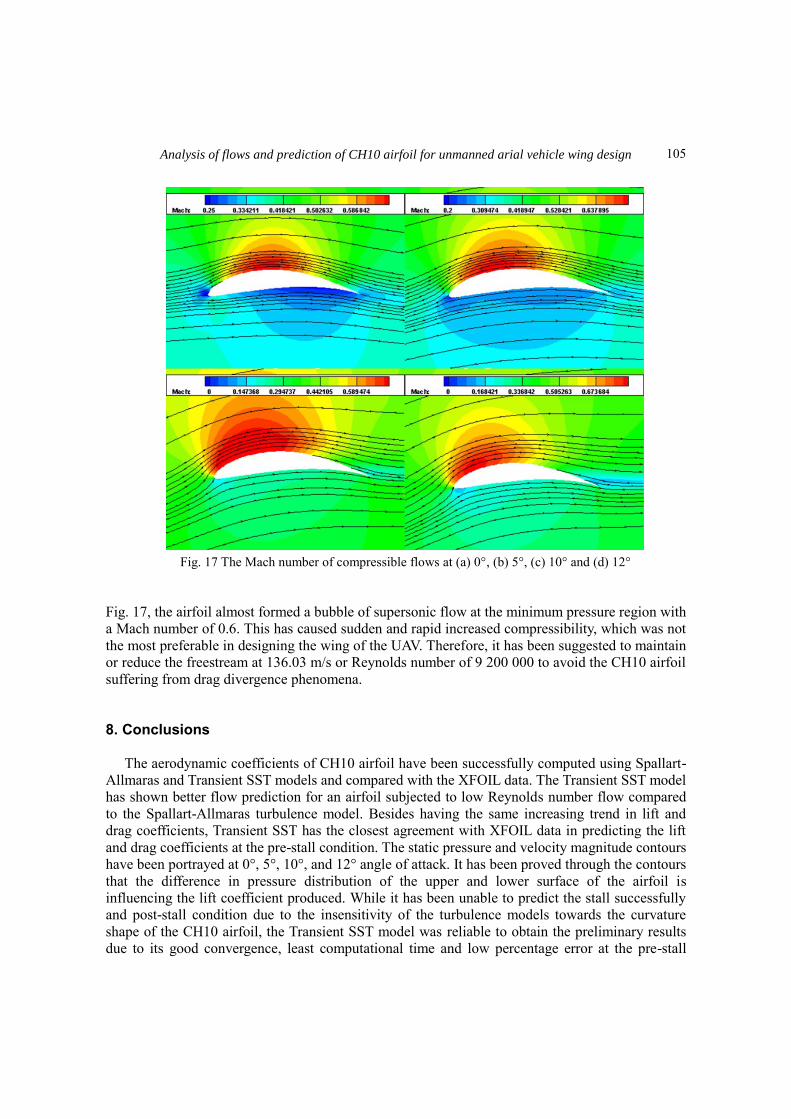
Fig. 17 The Mach number of compressible flows at (a) 0°, (b) 5°, (c) 10° and (d) 12°

Fig. 17, the airfoil almost formed a bubble of supersonic flow at the minimum pressure region with

a Mach number of 0.6. This has caused sudden and rapid increased compressibility, which was not

the most preferable in designing the wing of the UAV. Therefore, it has been suggested to maintain

or reduce the freestream at 136.03 m/s or Reynolds number of 9 200 000 to avoid the CH10 airfoil

suffering from drag divergence phenomena.

8. Conclusions

The aerodynamic coefficients of CH10 airfoil have been successfully computed using Spallart-

Allmaras and Transient SST models and compared with the XFOIL data. The Transient SST model

has shown better flow prediction for an airfoil subjected to low Reynolds number flow compared

to the Spallart-Allmaras turbulence model. Besides having the same increasing trend in lift and

drag coefficients, Transient SST has the closest agreement with XFOIL data in predicting the lift

and drag coefficients at the pre-stall condition. The static pressure and velocity magnitude contours

have been portrayed at 0°, 5°, 10°, and 12° angle of attack. It has been proved through the contours

that the difference in pressure distribution of the upper and lower surface of the airfoil is

influencing the lift coefficient produced. While it has been unable to predict the stall successfully

and post-stall condition due to the insensitivity of the turbulence models towards the curvature

shape of the CH10 airfoil, the Transient SST model was reliable to obtain the preliminary results

due to its good convergence, least computational time and low percentage error at the pre-stall

105


conditions. For recommendations, a newly developed curvature-sensitive SST k-ω-v2 turbulence

model can be used to predict the stall accurately. The user-defined function can be implemented by

using the C programming language and incorporated into ANSYS Fluent software.

References

Abdullah, A., Roslan, A.A. and Omar, Z. (2018), “Comparative study of turbulent incompressible flow past

naca airfoils”, ARPN J. Eng. Appl. Sci., 13(21), 8527-8530.

Abid, R. (1993), “Evaluation of two-equation turbulence models for predicting transitional flows”, Int. J.

Eng. Sci., 31(6), 831-840.

Ahmed, T., Amin, M.T. and Islam, S.M.R. (2013), “Computational Study of Flow around a NACA 0012

wing flapped at different flap angles with varying mach numbers”, Global J. Res. Eng., 13(4), 5-15.

Akhtar, M. N., Bakar, E. A., Aabid, A. and Khan, S.A. (2019), “Numerical simulations of a CD nozzle and

the influence of the duct length”, Int. J. Innov. Technol. Explor. Eng., 8(9S2), 622-630.

Arif, M., Mohamed, R., Guven, U. and Yadav, R. (2019), “Flow separation control of NACA-2412 airfoil

with bio-inspired nose”, Aircr. Eng. Aerosp. Tec., 7, 1058-1066.

https://doi.org/10.1108/AEAT-06-2018-0175

Baldock, N. and Mokhtarzadeh-Dehghan, M.R. (2006), “A study of solar-powered, high-altitude unmanned

aerial vehicles”, Aircr. Eng. Aerosp. Tec., 78(3), 187-193. https://doi.org/10.1108/17488840610663648.

Bayliss, A. and Turkel, E. (1982), “Far-field boundary conditions for compressible flows”, J. Comput. Phys.,

48(2), 182-199. https://doi.org/10.1016/0021-9991(82)90046-8.

Bitencourt, L.O., Pogorzelski, G., Freitas, R.M. and Azevedo, J.L.F. (2011), “A CFD-based analysis of the

14-Bis aircraft aerodynamics and stability”, J. Aerosp. Technol. Manage., 3(2), 137-146.

https://doi.org/10.5028/jatm.2011.03021711

Botti, L., Paliwal, N., Conti, P., Antiga, L. and Meng, H. (2018), “Modeling hemodynamics in intracranial

aneurysms: Comparing the accuracy of CFD solvers based on finite element and finite volume schemes”,

Int. J. Numer. Meth. Biomed. Eng., 34(9), 1-13. https://doi.org/10.1002/cnm.3111.

Carmichael, B.H. (2018), Low Reynolds Number Airfoil Survey, 3336.

Catalano, P. and Tognaccini, R. (2010), “Turbulence modeling for low-Reynolds-number flows”, AIAA J.,

48(8), 1673-1685. https://doi.org/10.2514/1.J050067.

Cerra, D.F. and Katz, J. (2008), “Design of a high-lift, thick airfoil for unmanned aerial vehicle

applications”, J. Aircraft, 45(5), 1789-1793. https://doi.org/10.2514/1.36924.

Cook, W.A. and Oakes, W.R. (1982), “A survey of unstructured mesh generation technology”, Comput.

Mech. Eng., 67-72.

Ebrahimi, A., Hajipour, M. and Ghamkhar, K. (2018), “Dual-position excitation technique in flow control

over an airfoil at low speeds”, Int. J. Numer. Meth. Heat Fluid Flow.

https://doi.org/10.1108/HFF-05-2018-0195

Eftekhari, S. and Al-obaidi, A.S M. (2019), “Investigation of a NACA 0012 finite wing aerodynamics at low

Reynold’ s numbers and 0° to 90° angle of attack”, J. Aerosp. Technol. Manage., 11, 1-11.

https://doi.org/10.5028/jatm.v11.1023

El Gharbi, N., Absi, R., Benzaoui, A. and Bennacer, R. (2011), “An improved near-wall treatment for

turbulent channel flows”, Int. J. Comput. Fluid Dyn., 25(1), 41-46.

https://doi.org/10.1080/10618562.2011.554832

Eleni, D.C., Athanasios, T.I. and Dionissios, M.P. (2012), “Evaluation of the turbulence models for the

simulation of the flow over a National Advisory Committee for Aeronautics (NACA) 0012 Airfoil”, J.

Mech. Eng. Res., 4(3), 100-111. https://doi.org/10.5897/JMER11.074,

Forster, K.J. and White, T.R. (2014), “Numerical investigation into vortex generators on heavily cambered

wings”, AIAA J., 52(5), 1059-1071. https://doi.org/10.2514/1.J052529.

Gowda, A.S. (2019), “Comparison of aerodynamic performance of NACA 4412 and 2412 using

106


computational approach”, Int. J. Eng. Trends Technol., 67(4), 73-75.

Grabis, Michael M., and Ramesh K. Agarwal. (2019), “Computational fluid dynamics analysis of inverted

multi-element airfoils in ground effect”, Proceedings of the AIAA Scitech 2019 Forum, San Diego,

California, U.S.A., January.

He, W., Pérez, J.M., Yu, P. and Li, L.K. (2019), “Non-modal stability analysis of low-Re separated flow

around a NACA 4415 airfoil in ground effect”, Aerosp. Sci. Technol., 92, 269-279.

https://doi.org/10.1016/j.ast.2019.06.007.

Heinrich, M. and Schwarze, R. (2016), “Density-based solver for all Mach number flows”, Progress

Comput. Fluid Dyn., 16(5), 271-280.

Islam, M.T., Arefin, A.M.E., Masud, M. and Mourshed, M. (1980), “The effect of Reynolds number on the

performance of a modified NACA 2412 airfoil”, Proceedings of the International Conference on

Mechanical Engineering.

Ives, R., Keir, A.S., Bassey, E. and Hamad, F.A. (2018), “Investigation of the flow around an aircraft wing of

Section NACA 2412 utilizing ANSYS fluent”, Proceedings of the Aerospace Europe CEAS 2017

Conference, Bucharest, Romania, October.

Jeong, W. and Seong, J. (2014), “Comparison of effects on technical variances of computational fluid

dynamics (CFD) software based on finite element and finite volume methods”, Int. J. Mech. Sci., 78, 19-

26. https://doi.org/10.1016/j.ijmecsci.2013.10.017.

Kandwal, S. and Singh, S. (2012), “Computational fluid dynamics study of fluid flow and aerodynamic

forces on an airfoil”, Int. J. Eng. Res. Technol., 1(7), 1-8.

Khan, S.A., Aabid, A., Ghasi, F.A.M., Al-Robaian, A.A. and Alsagri, A S. (2019), “Analysis of area ratio in a

CD nozzle with suddenly expanded duct using CFD method”, CFD Lett., 11(5), 61-71.

Kharati-koopaee, M. and Fallahzadeh-abarghooee, M. (2018), “Effect of corrugated skins on the

aerodynamic performance of the cambered airfoils”, Eng. Comput., 35(3), 1567-1582.

https://doi.org/10.1108/EC-08-2017-0302.

Kharulaman, L., Aabid, A., Ahmed, F., Mehaboobali, G. and Khan, S.A. (2019), “Research on flows for

NACA 2412 airfoil using computational fluid dynamics method”, Int. J. Eng. Adv. Technol., 9(1), 5450-

5456. https://doi.org/10.35940/ijeat.A3085.109119.

Lafountain, C., Cohen, K. and Abdallah, S. (2012), “Use of XFOIL in the design of camber-controlled

morphing UAVs”, Comput. Appl. Eng. Ed., 20, 673-680. https://doi.org/10.1002/cae.20437.

Leary, J. (2010), “Mini-project report computational fluid dynamics analysis of a low-cost wind turbine”,

University of Sheffield, Sheffield, U.K. Lissaman, P.B.S. (1983), “Low-Reynolds-number-airfoils”, Ann. Rev. Fluid Mech., 15, 223-239.

https://doi.org/10.1146/annurev.fl.15.010183.001255.

Liu, S. and Qin, N. (2014), “Modeling roughness effects for transitional low Reynolds number aerofoil

flows”, J. Aerosp. Eng., 229(2), 280-289. https://doi.org/10.1177/0954410014530875.

Lomax, H., Pulliam, T.H. and Zingg, D.W. (2013), Fundamentals of Computational Fluid Dynamics,

Springer Science& Business Media.

Lopes, A.M.G. (2016), “A 2D software system for expedite analysis of CFD problems in complex

geometries”, Comput. Appl. Eng. Ed., 24(1), 27-38. https://doi.org/10.1002/cae.21668.

Madhanraj, V.R. and Shah, D.A. (2019), “CFD analysis of NACA 2421 aerofoil at several angles of attack”,

J. Aeronaut. Aerosp. Eng., 8(1), 1-4.

Manni, L., Nishino, T. and Delafin, P. (2016), “Numerical study of airfoil stall cells using a very wide

computational domain”, Comput. Fluids, 140, 260-269. https://doi.org/10.1016/j.compfluid.2016.09.023.

Mamouri, A.R., Lakzian, E. and Khoshnevis, A. B. (2019), “Entropy analysis of pitching airfoil for offshore

wind turbines in the dynamic stall condition”, Ocean Eng., 187, 106229.

https://doi.org/10.1016/j.oceaneng.2019.106229.

Menon, K. and Mittal, R. (2020), “Aerodynamic characteristics of canonical airfoils at low Reynolds

numbers”, AIAA J., 58(2), 977-980. https://doi.org/10.2514/1.J058969.

Mermer, E., Koker, A., Kurtulus, D. F., Yilmaz, E. and Uzay, T. (2015), “Design and performance of wing

configurations for high altitude solar powered unmanned”, Proceedings of the Ankara International

107


Aerospace Conference, Ankara, Turkey, September.

Merryisha, S. and Rajendran, P. (2019), CFD Validation of NACA 2412 Airfoil.

Molina-Aiz, F.D., Fatnassi, H., Boulard, T., Roy, J.C. and Valera, D.L. (2010), “Comparison of finite

element and finite volume methods for simulation of natural ventilation in greenhouses”, Comput.

Electron. Agricult., 72(2), 69-86. https://doi.org/10.1016/j.compag.2010.03.002.

Morgado, J. (2016), “XFOIL vs. CFD performance predictions for high lift low Reynolds number airfoils”,

Aerosp. Sci. Technol., 52, 207-214. https://doi.org/10.1016/j.ast.2016.02.031

Myers, S.H. and Walters, D.K. (2005), “A one-dimensional subgrid near wall treatment for turbulent flow

CFD simulation”, Proceedings of the International Mechanical Engineering Congress and Exposition,

Orlando, Florida, U.S.A., November.

Corrêa, P.C.P. and Barcelos, M.N.D. (2013), “Numerical simulation of airfoils applied to UAVs”, Therm.

Eng., 13(1), 9-12. https://doi.org/10.5380/reterm.v13i1.62058.

Park, J., Seol, Y., Cordier, F. and Noh, J. (2010), “A smoke visualization model for capturing surface-like

features”, Comput. Graphics, 29(8), 2352-2362. https://doi.org/10.1111/j.1467-8659.2010.01719.x.

Patel, K.S., Patel, S.B., Patel, U.B. and Ahuja, P.A.P. (2015), “CFD analysis of an aerofoil”, Int. J. Eng. Res.,

3(3), 154-158. https://doi.org/10.17950/ijer/v3s3/305.

Petinrin, M.O. and Onoja, V.A. (2017), “Computational study of aerodynamic flow over NACA 4412

airfoil”, British J. Appl. Sci. Technol., 21(3), 1-11. https://doi.org/10.9734/BJAST/2017/31893

Petrova, R. (2012). Finite Volume Method – Powerful Means of Engineering Design, InTech, Rijeka,

Croatia.

Premkartikkumar, S.R., Ashok, V., Bhabhra, A.R. and Beladiya, A. (2018), “Design and analysis of a new

airfoil for RC aircrafts and UAVs”, Int. J. Mech. Eng. Technol., 9(4), 52-60.

Reddy, K., Sri, B., Aneesh, P., Bhanu, K. and Natarajan, M. (2016), “Design analysis of solar-powered

unmanned aerial vehicle”, J. Aerosp. Technol. Manage., 8(4), 397-407.

https://doi.org/10.5028/jatm.v8i4.666.

Reza, M.M.S., Mahmood, S.A. and Iqbal, A. (2016), “Performance analysis and comparison of high lift

airfoil for low-speed unmanned aerial vehicle”, Proceedings of the International Conference on

Mechanical, Industrial and Energy Engineering 2016, Bangladesh, December.

Rizvi, Z.A. (2017), “A study to understand differential equations applied to aerodynamics using CFD

technique”, Int. J. Sci. Eng. Res., 8(2), 16-19.

Sadrehaghighi, I. (2019). Mesh Generation in CFD.

Sagat, C., Mane, P. and Gawali, B.S. (2012), “Experimental and CFD analysis of airfoil at low Reynolds

number”, Int. J. Mech. Eng. Robotics Res., 1(3), 277-283.

Sagmo, K.F., Bartl, J. and Saetran, L. (2016), “Numerical simulations of the NREL S826 airfoil Numerical

simulations of the NREL S826 airfoil”, J. Phys. Conf. Ser., 1-9.

https://doi.org/10.1088/1742-6596/753/8/082036.

Sahu, R. and Patnaik, B.S.V. (2011), “CFD simulation of momentum injection control past a streamlined

body”, Int. J. Numer. Meth. Heat Fluid Flow, 21(8), 980-1001.

https://doi.org/10.1108/09615531111177750.

Salazar-Jimenes, G., Lopez-Aguilar, H.A., Gomez, J.A., Chazao-Zaharias, A., Duerte-Moller, A. and Perez-

Hernandez, A. (2018), “Blended wing CFD analysis: Aerodynamic”, Int. J. Math. Comput. Simul., 12, 33-

43.

Salim, M.S. and Cheah, S.C. (2009), “Wall y+ strategy for dealing with wall-bounded turbulent flows”,

Proceedings of the International MultiConference of Engineers and Computer Scientists, Hong Kong,

March.

Saraf, A.K., Singh, M.P. and Chouhan, T.E.J.S. (2017), “Aerodynamics analysis of NACA 0012 airfoil using

CFD”, Int. J. Mech. Prod. Eng., 5(12), 21-25.

Sayed, M.A., Kandil, H.A. and Shaltot, A. (2012), “Aerodynamic analysis of different wind-turbine blade

profiles using finite-volume method”, Energ. Convers. Manage., 64, 541-550.

https://doi.org/10.1016/j.enconman.2012.05.030.

Seetharam, H.C., Rodgers, E.J. and Wentz Jr, W.H. (2019), “Experimental studies of flow separation of the

108


NACA 2412 airfoil at low speeds”, NASA-CR-197497, NASA Langley Research Center.

Selig, M.S. and Guglielmo, J.J. (2008), “High-lift low Reynolds number airfoil design”, J. Aircraft, 34(1),

72-79. https://doi.org/10.2514/2.2137.

Shen, C., Sun, F. and Xia, X. (2014), “Implementation of density-based solver for all speeds in the

framework of openFOAM”, Comput. Phys. Commun., 185(10), 2730-2741.

https://doi.org/10.1016/j.cpc.2014.06.009.

Sher Afghan Khan, Aabid, A. and Baig, M.A.A. (2018), “Design and fabrication of unmanned arial vehicle

for multi-mission tasks”, Int. J. Mech. Prod. Eng. Res. Develop., 8(4), 475-484.

https://doi.org/10.24247/ijmperdaug201849.

Šidlof, P. (2016), “CFD simulation of flow-induced vibration of an elastically supported airfoil”,

Proceedings of the Experimental Fluid Mechanics 2015, Prague, Czech Republic, November.

Sogukpinar, H. and Bozkurt, I. (2018), “Implementation of different turbulence models to find the proper

model to estimate the aerodynamic properties of airfoils”, AIP Conf. Proc., 1935, 020003.

https://doi.org/10.1063/1.5025957.

Tang, L., Introduction, I. and Algorithm, N. (2008), “Reynolds-averaged Navier-Stokes simulations of low-

Reynolds-number airfoil aerodynamics”, J. Aircraft, 45(3), 848-856. https://doi.org/10.2514/1.21995.

Velkova, C., Calderon, F. M., Branger, T. and Soulier, C. (2016), “The impact of different turbulence models

at ansys fluent over the aerodynamic characteristics of ultra-light wing airfoil NACA 2412 airfoil”, Days

Mech., 1-5.

Yang, H.Q. and Dudley, J. (2017), “High-order pressure-based solver for aeroacoustic simulations high-

order pressure-based Solver for aeroacoustics simulations”, Proceedings of the 19th AIAA/CEAS

Aeroacoustics Conference, Berlin, Germany, May.

Zhang, C., Sanjosé, M. and Moreau, S. (2018), “Improvement of the near wall treatment in large Eddy

simulation for aeroacoustic applications”, Proceedings of the 2018 AIAA/CEAS Aeroacoustics Conference,

Atlanta, Georgia, U.S.A., June.

Ziemer, S. and Stenz, G. (2012), “The case for open source software in aeronautics”, Aircr. Eng. Aerosp.

Tec., 84(3), 133-139. https://doi.org/10.1108/00022661211221987

Zorkipli, M.K.H.M. and Razak, N.A. (2017), “Simulation of aeroelastic system with aerodynamic

nonlinearity”, Proceedings of the International Conference on Vibration, Sound and System Dynamics,

Kuala Lumpur, Malaysia, August.

EC

109

Analysis of flows and prediction of CH10 airfoil for ...

Documents

Transcript of Analysis of flows and prediction of CH10 airfoil for ...