Analysis of Flow in a 3D Chamber and a 2D Spray Nozzle to ...
185
University of South Florida Scholar Commons Graduate eses and Dissertations Graduate School 11-8-2004 Analysis of Flow in a 3D Chamber and a 2D Spray Nozzle to Approximate the Exiting Jet Free Surface Chin Tung Hong University of South Florida Follow this and additional works at: hps://scholarcommons.usf.edu/etd Part of the American Studies Commons is esis is brought to you for free and open access by the Graduate School at Scholar Commons. It has been accepted for inclusion in Graduate eses and Dissertations by an authorized administrator of Scholar Commons. For more information, please contact [email protected]. Scholar Commons Citation Hong, Chin Tung, "Analysis of Flow in a 3D Chamber and a 2D Spray Nozzle to Approximate the Exiting Jet Free Surface" (2004). Graduate eses and Dissertations. hps://scholarcommons.usf.edu/etd/1083
Transcript of Analysis of Flow in a 3D Chamber and a 2D Spray Nozzle to ...
University of South FloridaScholar Commons
Graduate Theses and Dissertations Graduate School
11-8-2004
Analysis of Flow in a 3D Chamber and a 2D SprayNozzle to Approximate the Exiting Jet Free SurfaceChin Tung HongUniversity of South Florida
Follow this and additional works at: https://scholarcommons.usf.edu/etd
Part of the American Studies Commons
This Thesis is brought to you for free and open access by the Graduate School at Scholar Commons. It has been accepted for inclusion in GraduateTheses and Dissertations by an authorized administrator of Scholar Commons. For more information, please contact [email protected].
Scholar Commons CitationHong, Chin Tung, "Analysis of Flow in a 3D Chamber and a 2D Spray Nozzle to Approximate the Exiting Jet Free Surface" (2004).Graduate Theses and Dissertations.https://scholarcommons.usf.edu/etd/1083
1
Analysis of Flow in a 3D Chamber and a 2D Spray Nozzle
to Approximate the Exiting Jet Free Surface
by
Chin Tung Hong
A thesis submitted in partial fulfillment of the requirements for the degree of
Master of Science in Mechanical Engineering Department of Mechanical Engineering
College of Engineering University of South Florida
Major Professor: Muhammad M. Rahman, Ph.D. Thomas Eason, Ph.D. Autar K. Kaw, Ph.D.
Date of Approval: November 8th, 2004
Keywords: spray cooling, cone angle, mixing length, liquid-gas interface, atomizer
© Copyright 2004, Chin Tung Hong
2
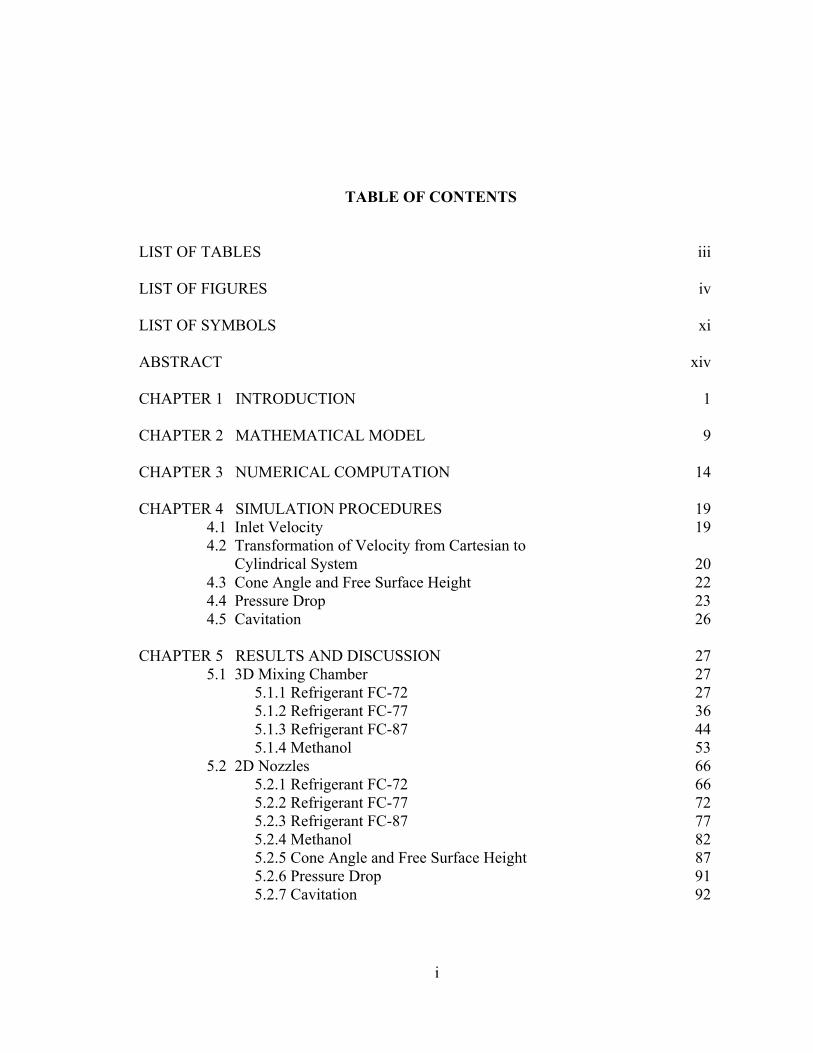
TABLE OF CONTENTS
LIST OF TABLES iii
LIST OF FIGURES iv
LIST OF SYMBOLS xi
ABSTRACT xiv
CHAPTER 1 INTRODUCTION 1
CHAPTER 2 MATHEMATICAL MODEL 9
CHAPTER 3 NUMERICAL COMPUTATION 14
CHAPTER 4 SIMULATION PROCEDURES 19
4.1 Inlet Velocity 19
4.2 Transformation of Velocity from Cartesian to Cylindrical System 20
4.3 Cone Angle and Free Surface Height 22 4.4 Pressure Drop 23 4.5 Cavitation 26
CHAPTER 5 RESULTS AND DISCUSSION 27 5.1 3D Mixing Chamber 27 5.1.1 Refrigerant FC-72 27 5.1.2 Refrigerant FC-77 36 5.1.3 Refrigerant FC-87 44 5.1.4 Methanol 53 5.2 2D Nozzles 66 5.2.1 Refrigerant FC-72 66 5.2.2 Refrigerant FC-77 72 5.2.3 Refrigerant FC-87 77 5.2.4 Methanol 82 5.2.5 Cone Angle and Free Surface Height 87 5.2.6 Pressure Drop 91 5.2.7 Cavitation 92
i
ii
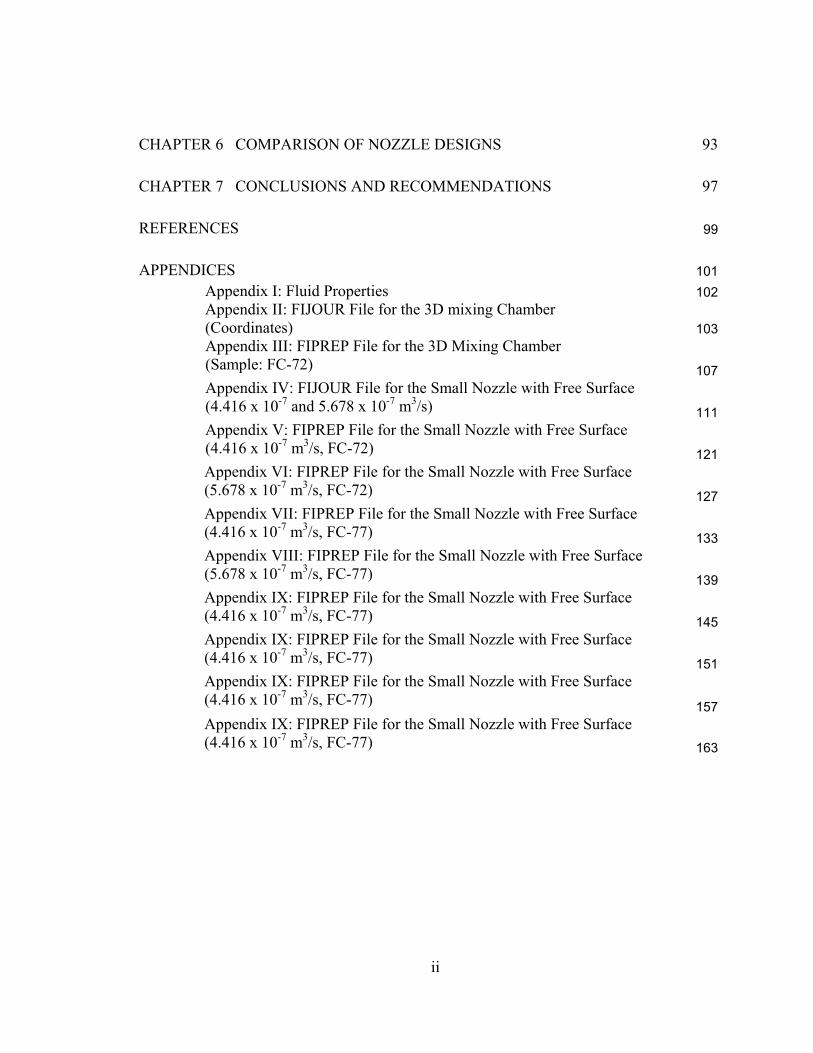
CHAPTER 6 COMPARISON OF NOZZLE DESIGNS 93
CHAPTER 7 CONCLUSIONS AND RECOMMENDATIONS 97
REFERENCES 99
APPENDICES 101 Appendix I: Fluid Properties 102
Appendix II: FIJOUR File for the 3D mixing Chamber (Coordinates) 103
Appendix III: FIPREP File for the 3D Mixing Chamber (Sample: FC-72) 107
Appendix IV: FIJOUR File for the Small Nozzle with Free Surface (4.416 x 10⁻⁷ and 5.678 x 10⁻⁷ m3/s) 111
Appendix V: FIPREP File for the Small Nozzle with Free Surface (4.416 x 10⁻⁷ m3/s, FC-72) 121
Appendix VI: FIPREP File for the Small Nozzle with Free Surface (5.678 x 10⁻⁷ m3/s, FC-72) 127
Appendix VII: FIPREP File for the Small Nozzle with Free Surface (4.416 x 10⁻⁷ m3/s, FC-77) 133
Appendix VIII: FIPREP File for the Small Nozzle with Free Surface (5.678 x 10⁻⁷ m3/s, FC-77) 139
Appendix IX: FIPREP File for the Small Nozzle with Free Surface (4.416 x 10⁻⁷ m3/s, FC-77) 145
Appendix IX: FIPREP File for the Small Nozzle with Free Surface (4.416 x 10⁻⁷ m3/s, FC-77) 151
Appendix IX: FIPREP File for the Small Nozzle with Free Surface (4.416 x 10⁻⁷ m3/s, FC-77) 157
Appendix IX: FIPREP File for the Small Nozzle with Free Surface (4.416 x 10⁻⁷ m3/s, FC-77) 163

iii
LIST OF TABLES
Table 1: Inlet velocity for different volumetric flow rates. 9 Table 2: The boundary conditions applied to the 3D chamber model. 12 Table 3:
The initial conditions and boundary conditions applied to the 2D spray nozzle model. 13
Table 4: Physical properties of working fluids in this analysis. 13 Table 5: Results of velocity transformation in four different axes. 22
Table 6: Cone angle and free surface height for each working fluid at various flow rates. 87
Table 7:
Cone angle, free surface height, and Reynolds number at the nozzle outlet for each working fluid (Q = 4.416 x 10⁻⁷ m3/s). 88
Table 8:
Cone angle, free surface height, and Reynolds number at the nozzle outlet for each working fluid (Q = 5.678 x 10⁻⁷ m3/s). 88
Table 9: Comparison of the working fluids pressure drop calculated using
Bernoulli’s equation and FIDAP simulation (Q= 4.416 x 10⁻⁷m3/s). 91
Table 10: 91
Comparison of the working fluids pressure drop calculated using Bernoulli’s equation and FIDAP simulation (Q= 5.678 x 10⁻⁷m3/s).
92 Table 11: Cavitation number of various refrigerants at different Reynolds numbers.
Table 12:
Cone angle and free surface height for each working fluid at various flow rates of the nozzle with outer slot radius 4.43 x 10⁻⁴ m. 96
iv
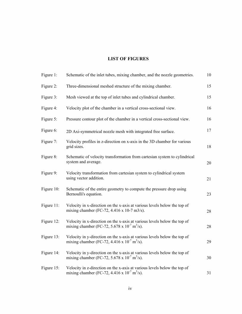
LIST OF FIGURES
Figure 1: 10
Schematic of the inlet tubes, mixing chamber, and the nozzle geometries.
Figure 2: Three-dimensional meshed structure of the mixing chamber. 15 Figure 3: Mesh viewed at the top of inlet tubes and cylindrical chamber. 15 Figure 4: Velocity plot of the chamber in a vertical cross-sectional view. 16 Figure 5: 16
Pressure contour plot of the chamber in a vertical cross-sectional view.
Figure 6: 2D Axi-symmetrical nozzle mesh with integrated free surface. 17
18
Figure 7:
Velocity profiles in z-direction on x-axis in the 3D chamber for various grid sizes.
Figure 8: 20
Schematic of velocity transformation from cartesian system to cylindrical system and average.
Figure 9: 21
Velocity transformation from cartesian system to cylindrical system using vector addition.
Figure 10:
23
Schematic of the entire geometry to compute the pressure drop using Bernoulli's equation.
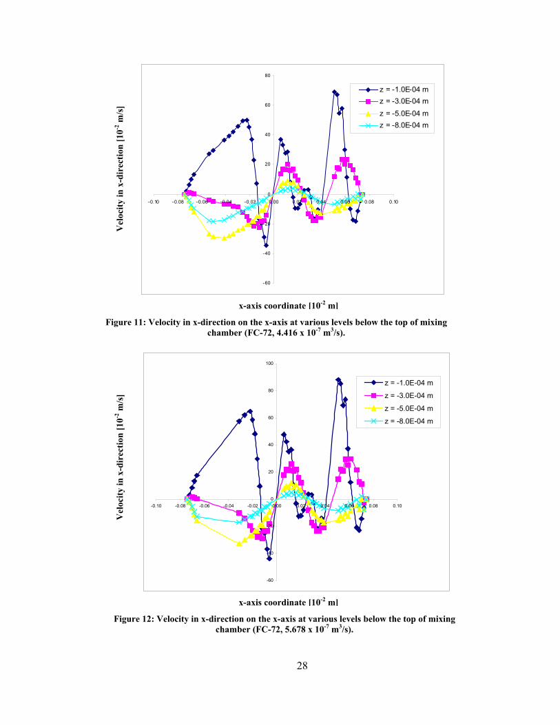
Figure 11: 28
Velocity in x-direction on the x-axis at various levels below the top of mixing chamber (FC-72, 4.416 x 10⁻⁷ m3/s).
Figure 12:
28
Velocity in x-direction on the x-axis at various levels below the top of mixing chamber (FC-72, 5.678 x 10⁻⁷ m3/s).
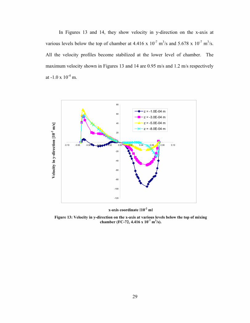
Figure 13:
29
Velocity in y-direction on the x-axis at various levels below the top of mixing chamber (FC-72, 4.416 x 10⁻⁷ m3/s).
Figure 14:
30
Velocity in y-direction on the x-axis at various levels below the top of mixing chamber (FC-72, 5.678 x 10⁻⁷ m3/s).
Figure 15:
Velocity in z-direction on the x-axis at various levels below the top of mixing chamber (FC-72, 4.416 x 10⁻⁷ m3/s).
31
v
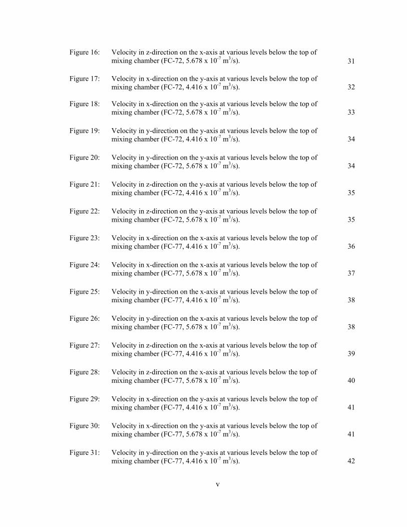
Figure 16: 31
Velocity in z-direction on the x-axis at various levels below the top of mixing chamber (FC-72, 5.678 x 10⁻⁷ m3/s).
Figure 17:
32
Velocity in x-direction on the y-axis at various levels below the top of mixing chamber (FC-72, 4.416 x 10⁻⁷ m3/s).
Figure 18:
33
Velocity in x-direction on the y-axis at various levels below the top of mixing chamber (FC-72, 5.678 x 10⁻⁷ m3/s).
Figure 19:
34
Velocity in y-direction on the y-axis at various levels below the top of mixing chamber (FC-72, 4.416 x 10⁻⁷ m3/s).
Figure 20:
34
Velocity in y-direction on the y-axis at various levels below the top of mixing chamber (FC-72, 5.678 x 10⁻⁷ m3/s).
Figure 21:
35
Velocity in z-direction on the y-axis at various levels below the top of mixing chamber (FC-72, 4.416 x 10⁻⁷ m3/s).
Figure 22:
35
Velocity in z-direction on the y-axis at various levels below the top of mixing chamber (FC-72, 5.678 x 10⁻⁷ m3/s).
Figure 23:
36
Velocity in x-direction on the x-axis at various levels below the top of mixing chamber (FC-77, 4.416 x 10⁻⁷ m3/s).
Figure 24:
37
Velocity in x-direction on the x-axis at various levels below the top of mixing chamber (FC-77, 5.678 x 10⁻⁷ m3/s).
Figure 25:
38
Velocity in y-direction on the x-axis at various levels below the top of mixing chamber (FC-77, 4.416 x 10⁻⁷ m3/s).
Figure 26:
38
Velocity in y-direction on the x-axis at various levels below the top of mixing chamber (FC-77, 5.678 x 10⁻⁷ m3/s).
Figure 27:
39
Velocity in z-direction on the x-axis at various levels below the top of mixing chamber (FC-77, 4.416 x 10⁻⁷ m3/s).
Figure 28:
40
Velocity in z-direction on the x-axis at various levels below the top of mixing chamber (FC-77, 5.678 x 10⁻⁷ m3/s).
Figure 29:
41
Velocity in x-direction on the y-axis at various levels below the top of mixing chamber (FC-77, 4.416 x 10⁻⁷ m3/s).
Figure 30:
41
Velocity in x-direction on the y-axis at various levels below the top of mixing chamber (FC-77, 5.678 x 10⁻⁷ m3/s).
Figure 31:
42
Velocity in y-direction on the y-axis at various levels below the top of mixing chamber (FC-77, 4.416 x 10⁻⁷ m3/s).
vi
Figure 32:
Velocity in y-direction on the y-axis at various levels below the top of mixing chamber (FC-77, 5.678 x 10⁻⁷ m3/s). 42
Figure 33: 43
Velocity in z-direction on the y-axis at various levels below the top of mixing chamber (FC-77, 4.416 x 10⁻⁷ m3/s).
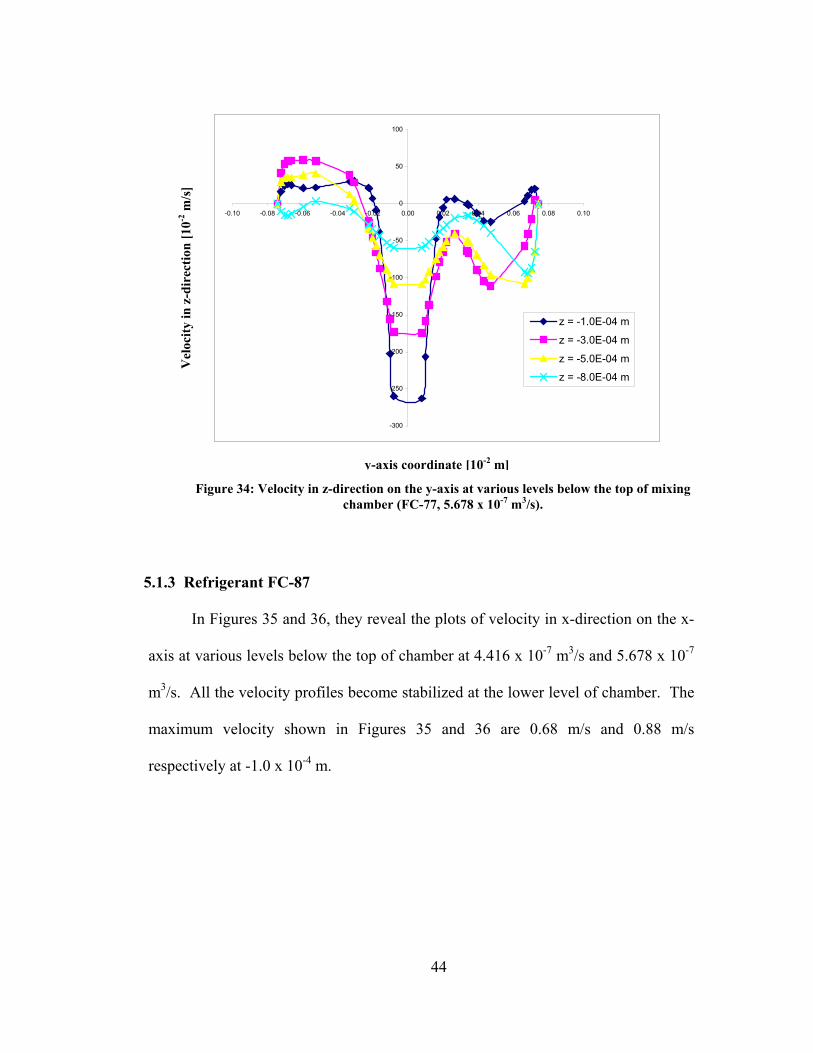
Figure 34:
44
Velocity in z-direction on the y-axis at various levels below the top of mixing chamber (FC-77, 5.678 x 10⁻⁷ m3/s).
Figure 35:
45
Velocity in x-direction on the x-axis at various levels below the top of mixing chamber (FC-87, 4.416 x 10⁻⁷ m3/s).
Figure 36:
45
Velocity in x-direction on the x-axis at various levels below the top of mixing chamber (FC-87, 5.678 x 10⁻⁷ m3/s).
Figure 37:
46
Velocity in y-direction on the x-axis at various levels below the top of mixing chamber (FC-87, 4.416 x 10⁻⁷ m3/s).
Figure 38:
47
Velocity in y-direction on the x-axis at various levels below the top of mixing chamber (FC-87, 5.678 x 10⁻⁷ m3/s).
Figure 39:
48
Velocity in z-direction on the x-axis at various levels below the top of mixing chamber (FC-87, 4.416 x 10⁻⁷ m3/s).
Figure 40:
48
Velocity in z-direction on the x-axis at various levels below the top of mixing chamber (FC-87, 5.678 x 10⁻⁷ m3/s).
Figure 41:
49
Velocity in x-direction on the y-axis at various levels below the top of mixing chamber (FC-87, 4.416 x 10⁻⁷ m3/s).
Figure 42:
50
Velocity in x-direction on the y-axis at various levels below the top of mixing chamber (FC-87, 5.678 x 10⁻⁷ m3/s).
Figure 43:
51
Velocity in y-direction on the y-axis at various levels below the top of mixing chamber (FC-87, 4.416 x 10⁻⁷ m3/s).
Figure 44:
51
Velocity in y-direction on the y-axis at various levels below the top of mixing chamber (FC-87, 5.678 x 10⁻⁷ m3/s).
Figure 45:
52
Velocity in z-direction on the y-axis at various levels below the top of mixing chamber (FC-87, 4.416 x 10⁻⁷ m3/s).
Figure 46:
52
Velocity in z-direction on the y-axis at various levels below the top of mixing chamber (FC-87, 5.678 x 10⁻⁷ m3/s).
Figure 47:
53
Velocity in x-direction on the x-axis at various levels below the top of mixing chamber (Methanol, 4.416 x 10⁻⁷ m3/s).
vii
Figure 48: 54
Velocity in x-direction on the x-axis at various levels below the top of mixing chamber (Methanol, 5.678 x 10⁻⁷ m3/s).
55
Figure 49: Velocity in y-direction on the x-axis at various levels below the top of mixing chamber (Methanol, 4.416 x 10⁻⁷ m3/s).
Figure 50:
55
Velocity in y-direction on the x-axis at various levels below the top of mixing chamber (Methanol, 5.678 x 10⁻⁷ m3/s).
Figure 51:
56
Velocity in z-direction on the x-axis at various levels below the top of mixing chamber (Methanol, 4.416 x 10⁻⁷ m3/s).
Figure 52:
56
Velocity in z-direction on the x-axis at various levels below the top of mixing chamber (Methanol, 5.678 x 10⁻⁷ m3/s).
Figure 53:
57
Velocity in x-direction on the y-axis at various levels below the top of mixing chamber (Methanol, 4.416 x 10⁻⁷ m3/s).
Figure 54:
58
Velocity in x-direction on the y-axis at various levels below the top of mixing chamber (Methanol, 5.678 x 10⁻⁷ m3/s).
Figure 55:
59
Velocity in y-direction on the y-axis at various levels below the top of mixing chamber (Methanol, 4.416 x 10⁻⁷ m3/s).
Figure 56:
59
Velocity in y-direction on the y-axis at various levels below the top of mixing chamber (Methanol, 5.678 x 10⁻⁷ m3/s).
Figure 57:
60
Velocity in z-direction on the y-axis at various levels below the top of mixing chamber (Methanol, 4.416 x 10⁻⁷ m3/s).
Figure 58:
60
Velocity in z-direction on the y-axis at various levels below the top of mixing chamber (Methanol, 5.678 x 10⁻⁷ m3/s).
Figure 59:
62
Cross-sectional velocity plot at 8.0 x 10⁻⁴ m below the top of chamber to show the circulation of FC-72 (Q = 4.416 x 10⁻⁷ m3/s) in clockwise direction.
Figure 60:
62
Cross-sectional velocity plot at 8.0 x 10⁻⁴ m below the top of chamber to show the circulation of FC-72 (Q = 5.678 x 10⁻⁷ m3/s) in clockwise direction.
Figure 61:
63
Cross-sectional velocity plot at 8.0 x 10⁻⁴ m below the top of chamber to show the circulation of FC-77 (Q = 4.416 x 10⁻⁷ m3/s) in clockwise direction.
Figure 62: Cross-sectional velocity plot at 8.0 x 10⁻⁴ m below the top of chamber to show the circulation of FC-77 (Q = 5.678 x 10⁻⁷ m3/s) in clockwise direction. 63
viii
Figure 63: Cross-sectional velocity plot at 8.0 x 10⁻⁴ m below the top of chamber to show the circulation of FC-87 (Q = 4.416 x 10⁻⁷ m3/s) in clockwise direction. 64
Figure 64:
64
Cross-sectional velocity plot at 8.0 x 10⁻⁴ m below the top of chamber to show the circulation of FC-87 (Q = 5.678 x 10⁻⁷ m3/s) in clockwise direction.
65
Figure 65: Cross-sectional velocity plot at 8.0 x 10⁻⁴ m below the top of chamber to show the circulation of Methanol (Q = 4.416 x 10⁻⁷ m3/s) in clockwise direction.
Figure 66:
65
Cross-sectional velocity plot at 8.0 x 10⁻⁴ m below the top of chamber to show the circulation of Methanol (Q = 5.678 x 10⁻⁷ m3/s) in clockwise direction.
Figure 67: Velocity vector plot for FC-72 (Q = 4.416 x 10⁻⁷ m3/s).Units are cm/s. 66
Figure 68: 67
Pressure contour plot for FC-72 (Q = 4.416 x 10⁻⁷ m3/s). Units are gm/cm s2 (x101 Pa).
Figure 69: Streamline contour plot for FC-72 (Q = 4.416 x 10⁻⁷ m3/s). 68 Figure 70: Velocity vector plot for FC-72 (Q = 5.678 x 10⁻⁷ m3/s).Units are cm/s. 69
Figure 71: 70
Pressure contour plot for FC-72 (Q = 5.678 x 10⁻⁷ m3/s). Units are gm/cm s2 (x101 Pa).
Figure 72: Streamline contour plot for FC-72 (Q = 5.678 x 10⁻⁷ m3/s). 70 Figure 73: Free surface profile for FC-72 at various flow rates. 71 Figure 74: Magnified free surface profile for FC-72 at various flow rates. 71 Figure 75: Velocity vector plot for FC-77 (Q = 4.416 x 10⁻⁷ m3/s).Units are cm/s. 72
Figure 76: 73
Pressure contour plot for FC-77 (Q = 4.416 x 10⁻⁷ m3/s). Units are gm/cm s2 (x101 Pa).
Figure 77: Streamline contour plot for FC-77 (Q = 4.416 x 10⁻⁷ m3/s). 73 Figure 78: Velocity vector plot for FC-77 (Q = 5.678 x 10⁻⁷ m3/s).Units are cm/s. 74
Figure 79: Pressure contour plot for FC-77 (Q = 5.678 x 10⁻⁷ m3/s). Units are gm/cm s2 (x101 Pa).
75
ix
Figure 80: Streamline contour plot for FC-77 (Q = 5.678 x 10⁻⁷ m3/s). 75 Figure 81: Free surface profile for FC-77 at various flow rates. 76 Figure 82: Magnified free surface profile for FC-77 at various flow rates.
76
Figure 83: Velocity vector plot for FC-87 (Q = 4.416 x 10⁻⁷ m3/s).Units are cm/s. 77
Figure 84: 78
Pressure contour plot for FC-87 (Q = 4.416 x 10⁻⁷ m3/s). Units are gm/cm s2 (x101 Pa).
Figure 85: Streamline contour plot for FC-87 (Q = 4.416 x 10⁻⁷ m3/s). 78
Figure 86: Velocity vector plot for FC-87 (Q = 5.678 x 10⁻⁷ m3/s).Units are cm/s. 79
Figure 87: 80
Pressure contour plot for FC-87 (Q = 5.678 x 10⁻⁷ m3/s). Units are gm/cm s2 (x101 Pa).
Figure 88: Streamline contour plot for FC-87 (Q = 5.678 x 10⁻⁷ m3/s). 80 Figure 89: Free surface profile for FC-87 at various flow rates. 81 Figure 90: Magnified free surface profile for FC-87 at various flow rates. 81 Figure 91: Velocity vector plot for Methanol (Q = 4.416 x 10⁻⁷ m3/s).Units are cm/s. 82
Figure 92: 83
Pressure contour plot for Methanol (Q = 4.416 x 10⁻⁷ m3/s). Units are gm/cm s2 (x101 Pa).
Figure 93: Streamline contour plot for Methanol (Q = 4.416 x 10⁻⁷ m3/s). 83 Figure 94: Velocity vector plot for Methanol (Q = 5.678 x 10⁻⁷ m3/s).Units are cm/s. 84
Figure 95:
85
Pressure contour plot for Methanol (Q = 5.678 x 10⁻⁷ m3/s). Units are gm/cm s2 (x101 Pa).
Figure 96: Streamline contour plot for Methanol (Q = 5.678 x 10⁻⁷ m3/s). 85 Figure 97: Free surface profile for Methanol at various flow rates. 86
Figure 98: Magnified free surface profile for Methanol at various flow rates. 86 Figure 99: Free surface profile for various fluids (Q=4.416 x 10⁻⁷ m3/s). 88
x
Figure 100: 89
Magnified free surface profile for various fluids (Q=4.416 x 10⁻⁷ m3/s).
Figure 101: Free surface profile for various fluids (Q=5.678 x 10⁻⁷ m3/s). 89 Figure 102: Magnified free surface profile for various fluids (Q=5.678 x 10⁻⁷ m3/s).
90
Figure 103: 93
Schematic of the nozzle geometry with outer slot radius 4.43 x 10⁻⁴ m.
Figure 104:
94
Magnified free surface profiles comparison for FC-72 with two different nozzle designs (Q=4.416 x 10⁻⁷ m3/s).
Figure 105:
94
Magnified free surface profiles comparison for FC-87 with two different nozzle designs (Q=4.416 x 10⁻⁷ m3/s).
Figure 106:
95
Magnified free surface profiles comparison for Methanol with two different nozzle designs (Q=4.416 x 10⁻⁷ m3/s).
Figure 107:
95
Magnified free surface profiles comparison for FC-72 with two different nozzle designs (Q=5.678 x 10⁻⁷ m3/s).
96 Figure 108:
Magnified free surface profiles comparison for Methanol with two different nozzle designs (Q=5.678 x 10⁻⁷ m3/s).
xi
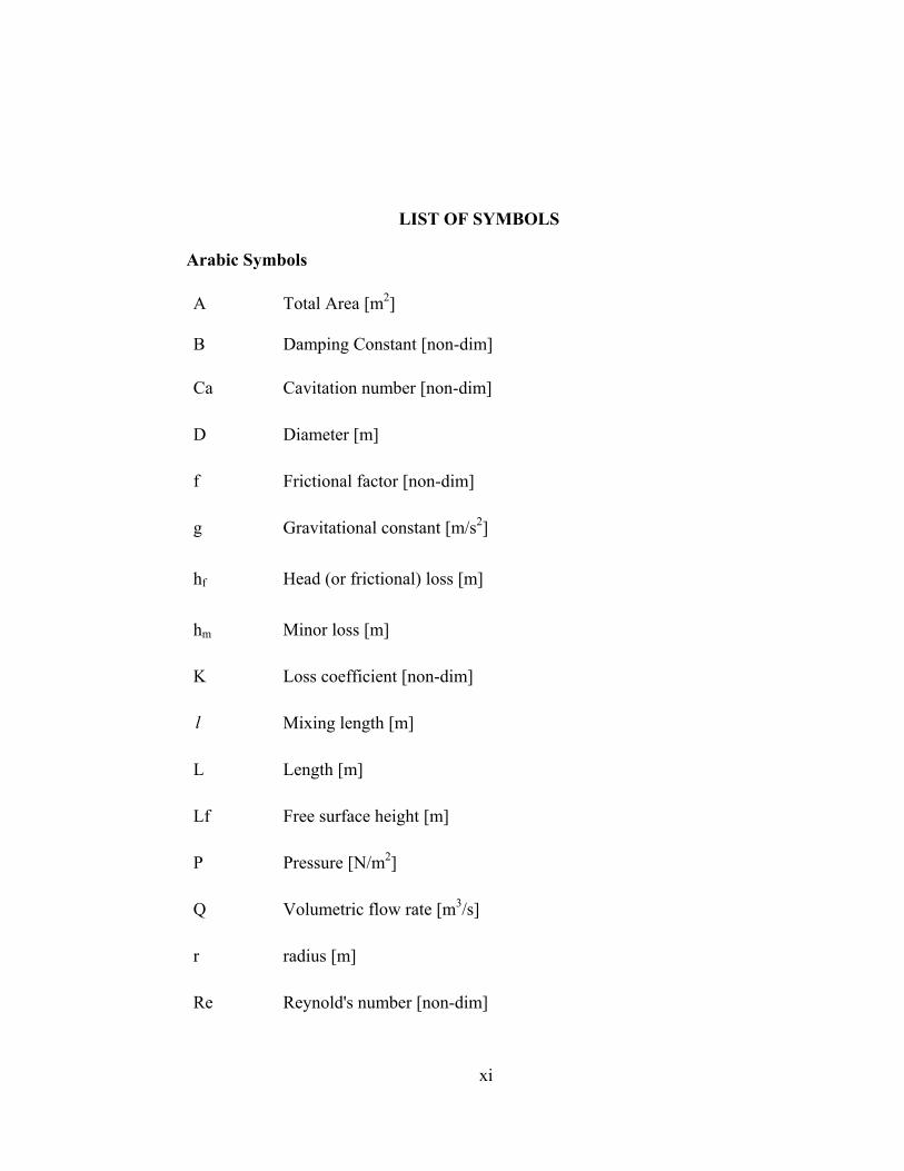
LIST OF SYMBOLS
Arabic Symbols A Total Area [m2] B Damping Constant [non-dim] Ca Cavitation number [non-dim] D Diameter [m] f Frictional factor [non-dim] g Gravitational constant [m/s2] hf Head (or frictional) loss [m] hm Minor loss [m] K Loss coefficient [non-dim] l Mixing length [m] L Length [m] Lf Free surface height [m] P Pressure [N/m2] Q Volumetric flow rate [m3/s] r radius [m] Re Reynold's number [non-dim]
xii
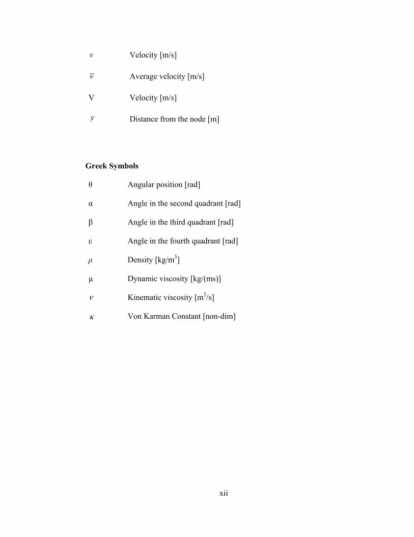
v Velocity [m/s] v Average velocity [m/s] V Velocity [m/s] y Distance from the node [m]
Greek Symbols θ Angular position [rad] α Angle in the second quadrant [rad] β Angle in the third quadrant [rad] ε Angle in the fourth quadrant [rad] ρ Density [kg/m3] µ Dynamic viscosity [kg/(ms)] ν Kinematic viscosity [m2/s] κ Von Karman Constant [non-dim]

xiii
Subscripts be Beveled outlet gc Gradual contraction n Normal direction r Radial direction t Turbulent x X-direction y Y-direction
z Axial or z-direction min Minimum sat Saturated θ, theta Circumferential

xiv
ANALYSIS OF FLOW IN A 3D CHAMBER AND A 2D SPRAY NOZZLE TO APPROXIMATE THE EXITING JET FREE SURFACE
Chin Tung Hong
ABSTRACT
The purpose of this investigation is to analyze the flow pattern of cooling
fluids in the 3D “twister-effect” mixing chamber and to approximate the free surface
behaviors exiting the 2D spray nozzle. The cone angle and free surface height
located at the end of the free surface are two significant factors to determine the
spraying area on a heated plane. This process is a reasonable representation of many
industrial cooling application. The whole system consists of 4 inlet tubes connected
to the top of the mixing chamber, and the spray nozzle is located under the chamber.
Four different refrigerants, like FC-72, FC-77, FC-87 and methanol were used for the
turbulent flow simulations. According to different fluid properties, the cone angle,
free surface, pressure drop and Reynolds number can be investigated at different
flow rates. First, at a certain volumetric flow rates, the velocities in x, y, z
directions were found on the positive x-axis (0 degree), y-axis (90 degrees), negative
x-axis (180 degrees) and y-axis (270 degrees) at 8.0 x 10⁻⁴ m below the top of
chamber. After the transformations, the interpolated and averaged radial,
circumferential and axial velocities were used in the 2D nozzle simulations. Finally,
the cone angle, the radial locations of the free surface and the pressure drop were
obtained in each scenario. As the results, higher volumetric flow rate produced
xv
higher free surface height and cone angle. Also, FC-87 created the highest free
surface height and cone angle among all four working fluids in both volumetric flow
rates. It means that FC-87 can produce the largest spraying area on the heated
surface. Fluctuation, spinning and eddy circulation can be found in the velocity plot
because of the turbulent flow syndromes. When comparing two different nozzle
designs, it was found that the nozzle without mixing chamber gave a larger cone
angle and free surface height. Alternatively, the design in this investigation produced
a relatively narrow jet concentrated to the stagnation zone.
xvi
CHAPTER 1
INTRODUCTION
Jet impingement or spray cooling is commonly used throughout the industry
for heat transfer applications, and also commonly studied by researchers because of
the high heat transfer rates that are achievable. It is used in a variety of applications
from the metal sheet industry to cooling of laser and electronic equipment. Also it is
frequently used in plastic film manufacturing, surface drying processes for paper,
cooling of fission and fusion components, and combustion walls and turbine blades
cooling. Micro spray cooling is also a new technology that may improve the cooling
efficiency of communications platforms installed on the unmanned aircraft and the
performance of the electronic drives for electric cars and train motors. Spray cooling
allows transistors to be driven harder and produce more power. Spray cooling also
enables chips to survive in harsh environments that would otherwise cause them to
fail.
Spray nozzle plays a very important role in the cooling of electronics.
Cooling electronic circuit integration is a vital part in maintaining the efficiency and
reliability of the circuitry. Undesirably high temperatures can severely strain the
operational safety and effectiveness of the electronics. Micro spray cooling
concentrates the spray to the hottest areas on a chip. Targeting the hottest areas on
the chip not only improves the heat removal capability but also minimizes the amount
1

2
of liquid required, making it more efficient from a system standpoint. To prevent the
cooling substance from affecting the electronics, the manufacturers coated the top
surface of silicon die with Parylene-C, a truly conformal polymer coating with
excellent dielectric properties. The polymer covers the sidewalls, trenches, and other
exposed surfaces on the chip.
At present, most of the electronic components are cooled by the heat sinks
attached to them and by blowing air with fans. Unfortunately, this technique does
not allow removing very high power without the heat sinks size becoming bulky or
the fan becoming too large. Conventionally, heat sinks and heat pipes touched down
on the chip were mechanically held to the chip surface. The heat, produced
uniformly over the postage stamp size surface area, diffused across the interface.
The interface produced significant temperature difference between the chip and the
heat sink. An even bigger limitation of direct air-cooling appears when dealing with
high heat fluxes, which are common since the chip’s size is becoming smaller by the
day. Because reliability and speed of any chip depend on the working temperature,
which is normally up to 120 degrees Celsius, new techniques are needed to improve
the heat removed per unit surface area and volume. However, before determining
the heat transfer properties of the system, it is important to determine the geometry
of the jet spray exiting the chamber and nozzle.
Prediction of nozzle performance for design and analysis is critical in helping
designers to meet effective and inexpensive performance. A set of design rules is
based on the experimentation with variable parameters of height, nozzle diameter,
and nozzle spacing in the submillmeter range. It can be used to develop an efficient
3
and economical heat exchanger that will meet present and future integrated circuit
microchip cooling requirements. The researchers mainly considered its ability to
transfer heat from the chip surface to a transport medium, usually air, and also the
medium’s heat capacity. A high-speed cool gas directly impinges on the hot surface
through MEMS nozzle or slot array, and penetrates deep into the boundary layer to
form a sharp temperature gradient. For instance, the cone angle of a particular spray
would be an important number to determine. A larger cone angle means that the
spray would be covering a greater surface area, and thus cooling a larger portion of
the electronics. Another important factor is how wide the spray becomes after it
exits the nozzle, or the radial height of the free surface. In addition, a greater radial
height produces more film surface area for the cooling purpose. A larger radial
height and cone angle of the free surface is beneficial, because this would indicate
that a greater fraction of the electronics would be cooled. This is significant for
efficiency, and consequently, the cost of the design.
The researchers recognized that a future microchip with multiple
functionalities would have some areas of high heat, low heat and no heat. Targeted
spray cooling is essential to avoid pooling. Using the re-engineered inkjet heads, the
researchers are able to target coolant spray to precise areas of the chip. The
mechanism sprays a measured amount of dielectric liquid coolant onto the chip
according to its heat level. The device controls the distribution, flow rate and
velocity of the liquid in much the same way inkjet printers control the placement of
ink on a printed page. The liquid vaporizes on impact, cooling the chip, and the
4
vapor is then passed through a heat exchanger and pumped back into a reservoir that
feeds the spray device.
One well-known method is phase-change cooling. Such phase change,
utilizing latent heat of vaporization of the liquid, removes significant heat flux.
However, as the pooled liquid changes phase, vapor bubbles form that adhere to the
wall of the chip. Also, the bubbles form really quickly in the dielectric fluids. At a
certain point on a tiny chip, a bubble will form on the hottest spots. If a bubble sits
on top, it becomes an insulator. At that point, heat transfer through the bubbles is
greatly limited, and the chip wall temperature quickly exceeds specifications. Laser
diodes, that are used greatly in nowadays communication applications, are very high
heat density sources, and it requires this type of cooling to maintain high working
efficiency.
It has been recognized that the nozzle design may affect the change in
geometry of the exiting spray. Jeng et al. (1998) performed experiments on 15
different nozzle geometries with four different flow rates and used the Arbitrary-
Langrangian-Eulerian (ALE) method to calculate the position of the free surface.
The finite element predictions were in good agreement with their experiments. They
concluded that the geometry of the nozzle had a significant effect on the parameters
of the exiting free surface that they were investigating.
Dumouchel et al. (1993) proposed that the nozzle geometry plays a major role
in the nozzle performance. They also applied numerical analysis to the velocity field
throughout a swirl spray nozzle, and more specifically, at the nozzle orifice. What
they found was that the conical liquid sheet produced at the nozzle’s orifice was
5
mainly dependent on the shape of the nozzle. Also an agreement with this statement
is Sakman et al. (2000). They studied the length-to-diameter ratio of the swirl
chamber and orifice, stating that an increase in the length-to-diameter ratio for both
the swirl chamber and orifice resulted in a decrease in the cone angle. However, an
increase in the length-to-diameter ratio for the swirl chamber produced an increase in
film thickness; an increase in the length-to-diameter ratio for the orifice resulted in a
decrease in the film thickness.
Miller and Ellis (2000) investigated spray nozzles for agricultural uses, mainly
focusing on spray characteristics and droplet size. They concluded that the
interaction between the physical properties of the spray liquid and the characteristics
of the spray formed was a function of the nozzle design. While some of the changes
in spray formation could be related to the dynamic surface tension of the spray
liquid, there was evidence to show that there were other physical parameters that
influenced spray formation. Som and Biswas (1986) agreed, stating that the
pertinent governing parameters regarding the spray dispersion included the liquid
velocity, liquid viscosity, liquid surface tension, the density of the ambient
atmosphere, as well as the geometrical dimensions of the nozzle.
Some other investigations were performed that observed the effect some
parameters had on the free surface position and the cone angle of the fluid exiting the
nozzle. Datta and Som (2000) studied ways to provide theoretical predictions of the
cone angle produced by swirl spray pressure nozzles using numerical computations
of the flow. They realized that an increase in the fluid flow rate created a sharp
increase in the cone angle of the fluid exiting the swirl nozzle. Rothe and Block
6
(1977) examined the effect that the pressure of the ambient environment to which the
fluid is being sprayed had on the shape of the liquid sheet. Their work, which agrees
with many other studies, found that an increase in ambient pressure and nozzle
pressure drop created an increase in contraction of the liquid sheet emanating from
the nozzle. However, an increase in nozzle diameter aided in decreasing the amount
of contraction.
Gavaises and Arcoumanis (2001) state that an accurate estimation of the
nozzle flow exit conditions are significant in the calculation of sprays ejected from
the nozzle. Therefore, it is important to know the conditions at the location where
the fluid exits the nozzle in order to truthfully predict the position of the free surface,
as well as other interesting variables. After the free surface of the fluid has been
modeled correctly, the heat transfer potential can then be evaluated. Ciofalo et al.
(1999) performed experiments with full cone swirl atomizers onto a heated wall.
They confirmed that the heat transfer coefficient and maximum heat flux was
dependent of the mass flux of the spray, as well as the droplet velocity.
Fabbri et al. (2003) concluded that the local heat transfer decreases sharply as
one moves radially outward from the stagnation region to the periphery. Also, the
major conclusions are that the jet impingement flow can be divided in four regions.
Region 1 is the stagnation zone where it was found that the thickness of the
hydrodynamic and thermal boundary layers is constant. In the second region, both
boundary layers are developing and none have reached the free surface. Region 3 is
characterized by the face that the hydrodynamic boundary layer has reached the free
surface, whereas the thermal boundary layer is still thinner than the film thickness.
7
Finally in region 4, both boundary layers have reached the free surface of the liquid
film.
Recently, attention has been focused on circular arrays of free surface micro
jets. The jet Reynolds number is the mostly concerned parameter. Micro
impinging jets can be highly efficient, found by Wu et al. (1999), when compared to
existing macro impinging-jet microelectronics packages. As the transistor density
and/or the number of transistors on a standard-sized chip increases in IC’s, the power
dissipation also increases. It is therefore necessary to investigate better thermal
cooling methods for future chip cooling. A more efficient micro heat exchanger
should be invented, as micro jets can be placed much closer to the hot surface than
conventional macro jets. The goal of their work was then to study micro impinging
jet cooling, focusing on experimentation with variable parameters of height, nozzle
diameter, and nozzle spacing in the sub-millimeter range. It is found that a micro
impinging jet can provide effective cooling. Higher driving pressure gives better
cooling, but lower efficiency. This tradeoff should be considered when using
MEMS impinging-jet heat exchangers.
Objectives
The objectives of this investigation are shown as the following:
1. To approximate the flow pattern of some refrigerants, such as FC-72, FC-77, FC-
87, and Methanol in this specially designed “twister-effect” mixing chamber and
spray nozzle.

8
2. To understand the relationship among cone angle, free surface height, pressure
drop, Reynolds number created in this nozzle with mixing chamber, and the fluid
properties.
3. To compare the results of the nozzle design in this investigation and one from
another.
9
CHAPTER 2
MATHEMATICAL MODEL
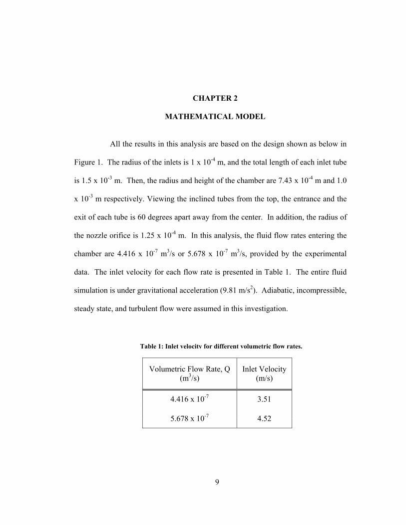
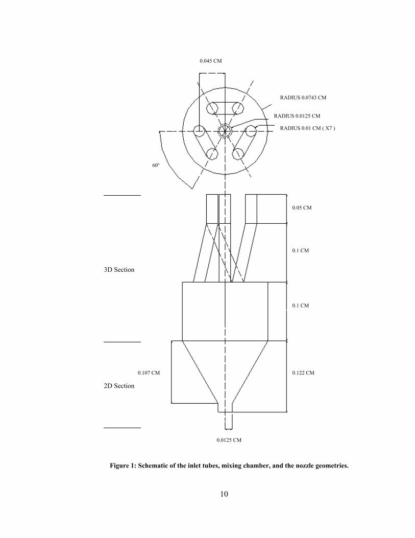
All the results in this analysis are based on the design shown as below in
Figure 1. The radius of the inlets is 1 x 10⁻⁴ m, and the total length of each inlet tube
is 1.5 x 10⁻³ m. Then, the radius and height of the chamber are 7.43 x 10⁻⁴ m and 1.0
x 10-3 m respectively. Viewing the inclined tubes from the top, the entrance and the
exit of each tube is 60 degrees apart away from the center. In addition, the radius of
the nozzle orifice is 1.25 x 10⁻⁴ m. In this analysis, the fluid flow rates entering the
chamber are 4.416 x 10⁻⁷ m3/s or 5.678 x 10⁻⁷ m3/s, provided by the experimental
data. The inlet velocity for each flow rate is presented in Table 1. The entire fluid
simulation is under gravitational acceleration (9.81 m/s2). Adiabatic, incompressible,
steady state, and turbulent flow were assumed in this investigation.
Volumetric Flow Rate, Q (m3/s)
Inlet Velocity (m/s)
4.416 x 10⁻⁷ 3.51
5.678 x 10⁻⁷ 4.52
Table 1: Inlet velocity for different volumetric flow rates.
10
Figure 1: Schematic of the inlet tubes, mixing chamber, and the nozzle geometries.
RADIUS 0.0743 CM
RADIUS 0.0125 CM
RADIUS 0.01 CM ( X7 )
0.045 CM
60°
0.05 CM
0.1 CM
0.1 CM
0.122 CM
0.0125 CM
0.107 CM
3D Section
2D Section
11
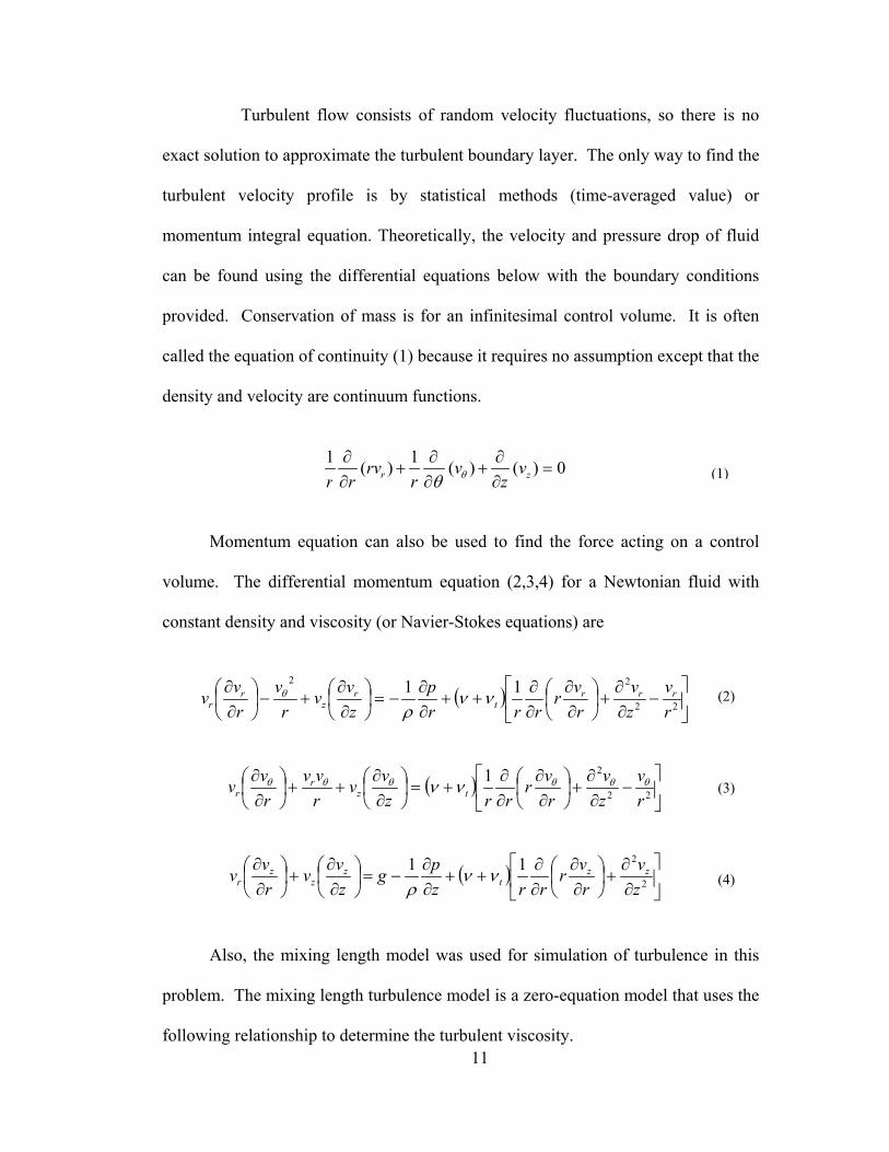
Turbulent flow consists of random velocity fluctuations, so there is no
exact solution to approximate the turbulent boundary layer. The only way to find the
turbulent velocity profile is by statistical methods (time-averaged value) or
momentum integral equation. Theoretically, the velocity and pressure drop of fluid
can be found using the differential equations below with the boundary conditions
provided. Conservation of mass is for an infinitesimal control volume. It is often
called the equation of continuity (1) because it requires no assumption except that the
density and velocity are continuum functions.
0)()(1)(1=
∂∂
+∂∂
+∂∂
zr vz
vr
rvrr θθ
Momentum equation can also be used to find the force acting on a control
volume. The differential momentum equation (2,3,4) for a Newtonian fluid with
constant density and viscosity (or Navier-Stokes equations) are
( )
−
∂∂
+
∂∂
∂∂
++∂∂
−=
∂∂
+−
∂∂
22
22 11rv
zv
rvr
rrrp
zvv
rv
rvv rrr
tr
zr
r ννρ
θ
( )
−
∂∂
+
∂∂
∂∂
+=
∂∂
++
∂∂
22
21rv
zv
rvr
rrzvv
rvv
rvv tz
rr
θθθθθθ νν
( )
∂∂
+
∂∂
∂∂
++∂∂
−=
∂∂
+
∂∂
2
211zv
rvr
rrzpg
zvv
rvv zz
tz
zz
r ννρ
Also, the mixing length model was used for simulation of turbulence in this
problem. The mixing length turbulence model is a zero-equation model that uses the
following relationship to determine the turbulent viscosity.
(1)
(2)
(3)
(4)
12
rvvl r
rt ∂∂⋅⋅= 2ν
−−⋅⋅=
+
By
yl nn exp1κ
where κ is the Von Karman constant (κ = 0.4), yn is the normal distance from the
node to the wall yn+ is a scale used to non-dimensionalize the problem, and B is the
damping constant. The Van Driest damping factor is located within the brackets [ ].
ν
*vyy nn
⋅=+
where v* is the friction velocity.
By applying the boundary conditions given in Tables 2 and 3 and the
assumption to the above mathematical models, the equation of continuity and
Navier-Stokes equations can be simplified. Also, the fluid properties in Table 4 can
also be used for the same purpose.
Location Boundary Conditions Inlets Velocity at the inlet depends on the volumetric flow rate.
Inlet walls Velocity is set to be zero. (Vx = Vy = Vz = 0) Top of the chamber Velocity is set to be zero. (Vx = Vy = Vz = 0)
Chamber wall Velocity is set to be zero. (Vx = Vy = Vz = 0)
Chamber outlet
All the velocities on each of the four axes resulted from the 3D simulation will be linearly interpolated and averaged, and they will then be used as the initial conditions and boundary conditions at the inlet of 2D nozzle.
(5)
(6)
(7)
Table 2: The boundary conditions applied to the 3D chamber model.
13
Location Initial Conditions and Boundary Conditions
Nozzle inlet Velocity at the inlet depends on the results at the 3D chamber outlet.
Nozzle wall Velocity is set to be zero. (Vr = Vtheta = Vz = 0) Axis of symmetry Radial velocity is set to be zero. (Vr = 0)
Refrigerants Type of Chemicals
Density [kg/m3]
Viscosity [kg/m-s]
Surface Tension [N/m]
FC-72 Fluorocarbon 1680 6.4 x 10⁻⁴ 0.01
FC-77 Fluorocarbon 1780 1.424 x 10⁻³ 0.015 FC-87 Fluorocarbon 1630 4.53 x 10⁻⁴ 0.0095
Methanol Hydrocarbon 785.5 5.5 x 10⁻⁴ 0.0222
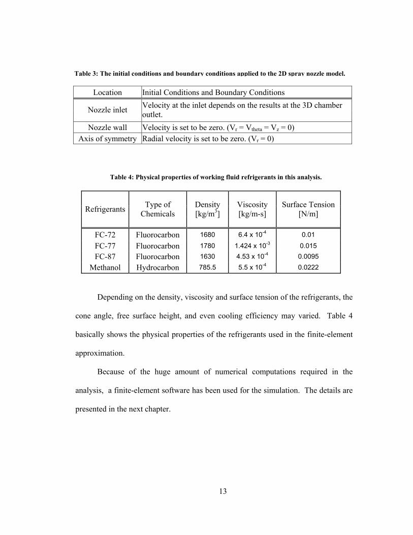
Depending on the density, viscosity and surface tension of the refrigerants, the
cone angle, free surface height, and even cooling efficiency may varied. Table 4
basically shows the physical properties of the refrigerants used in the finite-element
approximation.
Because of the huge amount of numerical computations required in the
analysis, a finite-element software has been used for the simulation. The details are
presented in the next chapter.
Table 3: The initial conditions and boundary conditions applied to the 2D spray nozzle model.
Table 4: Physical properties of working fluid refrigerants in this analysis.

14
CHAPTER 3
NUMERICAL COMPUTATION
Since the entire simulation requires tremendous amount of quadrilateral
elements, it is divided into a 3D mixing chamber portion and 2D axi-symmetrical
nozzle portion. They were both constructed and solved by a finite-element software
named FIDAP. During the production of this 3D mesh, boundary edges were applied
to guarantee the fine quality of mesh on each boundary surface. Pave and map
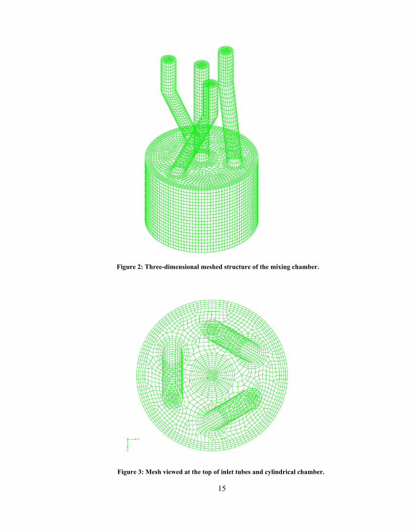
meshing method were used to construct the 3D chamber as shown in Figure 2 and
Figure 3. To achieve the higher accuracy in the 3D simulation, the number of
element was increased as much as the server can possibly handle. Segregated
method and steady state turbulent assumptions have been chosen to solve this 3D
chamber problem for the limited memory storage provided and short simulation
period. Eventually, some results were obtained as shown in Figures 4 and 5. Next,
the 2D nozzle was made by map meshing method because of its simple geometric
structure. Newton-Raphson was found to be the best method solving a 2D mixing
length turbulent free surface problem. In this case, the problem was set to be
transient as the change in free surface can be examined in each time step. Moreover,
to ensure the accuracy of computation at the dynamic regions, the 2D mesh, shown
in Figure 6, has been integrated by increasing the amount of element in where the
free surface started and ended. The grid size of the 2D mesh is 30 x 142.
15
Figure 2: Three-dimensional meshed structure of the mixing chamber.
Figure 3: Mesh viewed at the top of inlet tubes and cylindrical chamber.
16
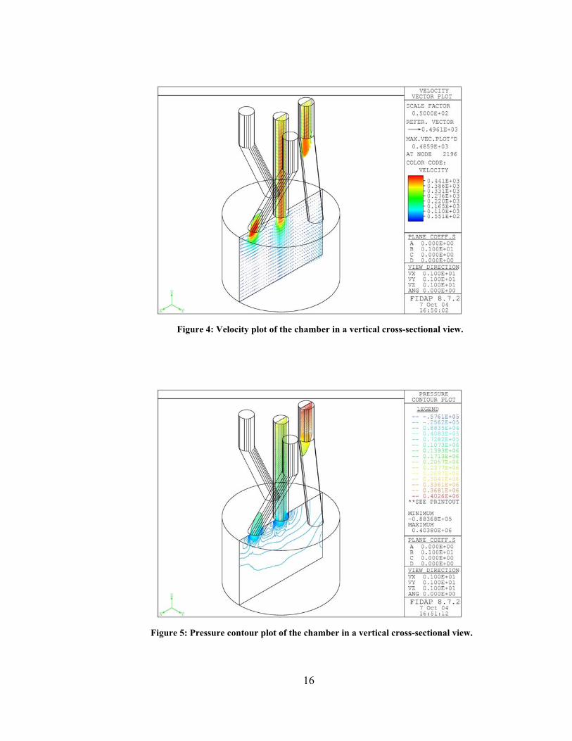
Figure 4: Velocity plot of the chamber in a vertical cross-sectional view.
Figure 5: Pressure contour plot of the chamber in a vertical cross-sectional view.
17
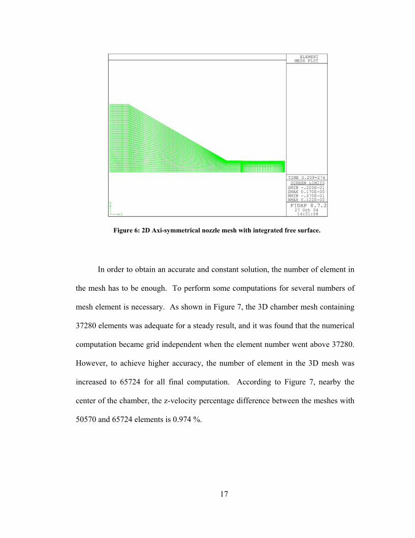
In order to obtain an accurate and constant solution, the number of element in
the mesh has to be enough. To perform some computations for several numbers of
mesh element is necessary. As shown in Figure 7, the 3D chamber mesh containing
37280 elements was adequate for a steady result, and it was found that the numerical
computation became grid independent when the element number went above 37280.
However, to achieve higher accuracy, the number of element in the 3D mesh was
increased to 65724 for all final computation. According to Figure 7, nearby the
center of the chamber, the z-velocity percentage difference between the meshes with
50570 and 65724 elements is 0.974 %.
Figure 6: 2D Axi-symmetrical nozzle mesh with integrated free surface.
18
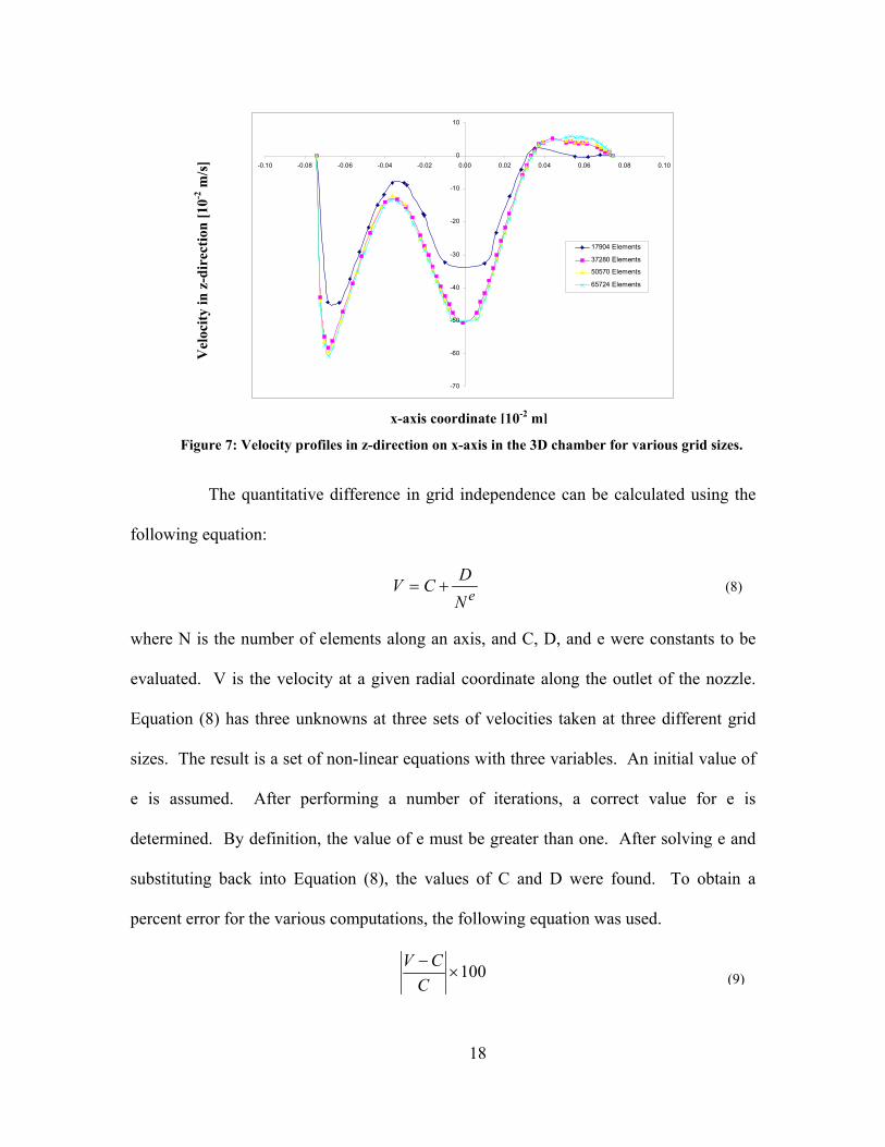
The quantitative difference in grid independence can be calculated using the
following equation:
eNDCV += (8)
where N is the number of elements along an axis, and C, D, and e were constants to be
evaluated. V is the velocity at a given radial coordinate along the outlet of the nozzle.
Equation (8) has three unknowns at three sets of velocities taken at three different grid
sizes. The result is a set of non-linear equations with three variables. An initial value of
e is assumed. After performing a number of iterations, a correct value for e is
determined. By definition, the value of e must be greater than one. After solving e and
substituting back into Equation (8), the values of C and D were found. To obtain a
percent error for the various computations, the following equation was used.
100×−C
CV
-70
-60
-50
-40
-30
-20
-10
0
10
-0.10 -0.08 -0.06 -0.04 -0.02 0.00 0.02 0.04 0.06 0.08 0.10
17904 Elements
37280 Elements
50570 Elements
65724 Elements
x-axis coordinate [10-2 m]
Figure 7: Velocity profiles in z-direction on x-axis in the 3D chamber for various grid sizes.
Vel
ocity
in z
-dir
ectio
n [1
0-2 m
/s]
(9)
19
CHAPTER 4
SIMULATION PROCEDURES
Before start working on this analysis, some preparations are needed to provide
enough information for the finite-element simulation. Also, manipulation of result
data is very important. As seen below, the simulation procedures are described in
detailed.
4.1 Inlet Velocity
To calculate the inlet velocity Vinlet, the cross-sectional area of all inlets is
needed.
)3( inclinedcentralinlet AAVQ +⋅=
where Q is the fluid volumetric flow rate.
There are four refrigerants (FC-72, FC-77, FC-87, and Methanol) at two
different flow rates (4.416 x 10⁻⁷ m3/s and 5.678 x 10⁻⁷ m3/s) in this work. After
providing the fluid properties and inlet velocity (see Appendix III), the 3D chamber
simulation was run until it reached steady state. Based on the Cartesian coordinate
system, the fluid sectional velocity was then obtained in four axial directions (+x, +y,
-x, and –y) only at 0.02 cm above the chamber exit and was then transferred to the
2D simulation (see Appendices IV to XII).
(10)
20
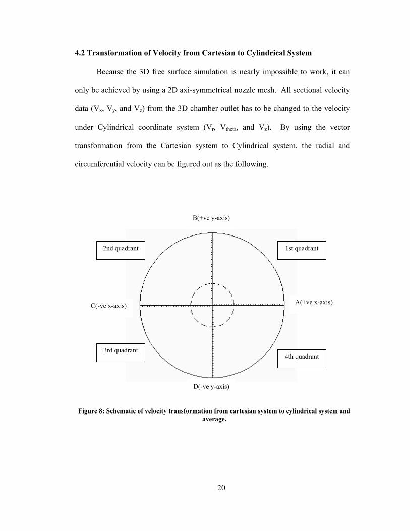
4.2 Transformation of Velocity from Cartesian to Cylindrical System
Because the 3D free surface simulation is nearly impossible to work, it can
only be achieved by using a 2D axi-symmetrical nozzle mesh. All sectional velocity
data (Vx, Vy, and Vz) from the 3D chamber outlet has to be changed to the velocity
under Cylindrical coordinate system (Vr, Vtheta, and Vz). By using the vector
transformation from the Cartesian system to Cylindrical system, the radial and
circumferential velocity can be figured out as the following.
1st quadrant 2nd quadrant
3rd quadrant 4th quadrant
B(+ve y-axis)
A(+ve x-axis)C(-ve x-axis)
D(-ve y-axis)
Figure 8: Schematic of velocity transformation from cartesian system to cylindrical system and average.
21
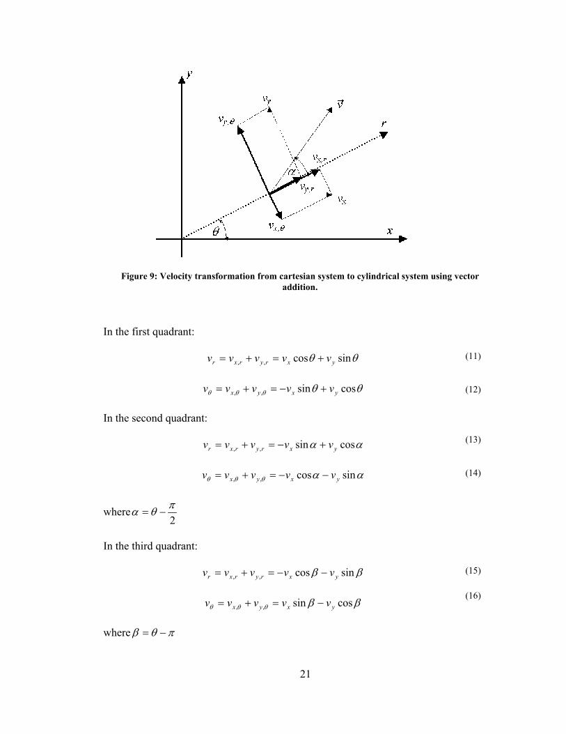
In the first quadrant:
θθ sincos,, yxryrxr vvvvv +=+=
θθθθθ cossin,, yxyx vvvvv +−=+=
In the second quadrant:
αα cossin,, yxryrxr vvvvv +−=+=
ααθθθ sincos,, yxyx vvvvv −−=+=
where2πθα −=
In the third quadrant:
ββ sincos,, yxryrxr vvvvv −−=+=
ββθθθ cossin,, yxyx vvvvv −=+=
where πθβ −=
Figure 9: Velocity transformation from cartesian system to cylindrical system using vector addition.
(11)
(12)
(13)
(14)
(15)
(16)
22
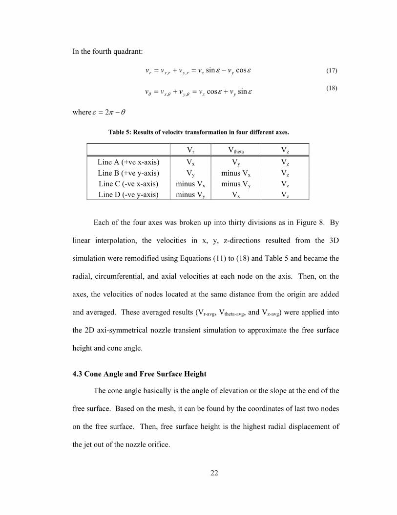
In the fourth quadrant:
εε cossin,, yxryrxr vvvvv −=+=
εεθθθ sincos,, yxyx vvvvv +=+=
where θπε −= 2
Vr Vtheta Vz Line A (+ve x-axis) Vx Vy Vz Line B (+ve y-axis) Vy minus Vx Vz Line C (-ve x-axis) minus Vx minus Vy Vz Line D (-ve y-axis) minus Vy Vx Vz
Each of the four axes was broken up into thirty divisions as in Figure 8. By
linear interpolation, the velocities in x, y, z-directions resulted from the 3D
simulation were remodified using Equations (11) to (18) and Table 5 and became the
radial, circumferential, and axial velocities at each node on the axis. Then, on the
axes, the velocities of nodes located at the same distance from the origin are added
and averaged. These averaged results (Vr-avg, Vtheta-avg, and Vz-avg) were applied into
the 2D axi-symmetrical nozzle transient simulation to approximate the free surface
height and cone angle.
4.3 Cone Angle and Free Surface Height
The cone angle basically is the angle of elevation or the slope at the end of the
free surface. Based on the mesh, it can be found by the coordinates of last two nodes
on the free surface. Then, free surface height is the highest radial displacement of
the jet out of the nozzle orifice.
Table 5: Results of velocity transformation in four different axes.
(17)
(18)

23
4.4 Pressure Drop
The pressure drop between the inlets above the mixing chamber and the outlet
of the nozzle is also important in this jet impingement analysis. The finite-element
software provided the pressure difference after the simulation. Nevertheless, the
pressure difference can be calculated by using Bernoulli’s Equations (22), (24), (27),
and (29). It was assumed that it was constant flow rate in the whole fluid simulation.
The nozzle was made of new stainless steel material that has 0.002 mm as the
roughness height. Because of the high inlet velocity, the flow was considered as
turbulent for the Bernoulli’s equation.
Figure 10: Schematic of the entire geometry to compute the pressure drop by Bernoulli’s equation.
Location A (1.5 x 10⁻³ m)
inlet
Location 1 (1.0 x 10⁻³ m)
Location 2 (0 m)
reference point
Location 3 (-1.0 x 10⁻³ m)
Location 4 (-1.7 x 10⁻³ m)
outlet
24
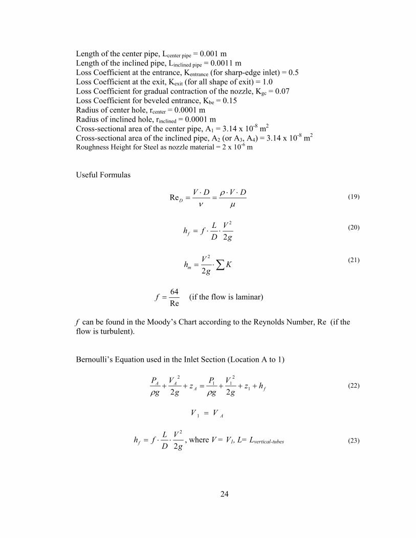
Length of the center pipe, Lcenter pipe = 0.001 m Length of the inclined pipe, Linclined pipe = 0.0011 m Loss Coefficient at the entrance, Kentrance (for sharp-edge inlet) = 0.5 Loss Coefficient at the exit, Kexit (for all shape of exit) = 1.0 Loss Coefficient for gradual contraction of the nozzle, Kgc = 0.07 Loss Coefficient for beveled entrance, Kbe = 0.15 Radius of center hole, rcenter = 0.0001 m Radius of inclined hole, rinclined = 0.0001 m Cross-sectional area of the center pipe, A1 = 3.14 x 10⁻⁸ m2 Cross-sectional area of the inclined pipe, A2 (or A3, A4) = 3.14 x 10⁻⁸ m2
Roughness Height for Steel as nozzle material = 2 x 10⁻⁶ m
Useful Formulas
µρ
νDVDV
D⋅⋅
=⋅
=Re
gV
DLfhf 2
2
⋅⋅=
∑⋅= Kg
Vhm 2
2
Re64
=f (if the flow is laminar)
f can be found in the Moody’s Chart according to the Reynolds Number, Re (if the flow is turbulent). Bernoulli’s Equation used in the Inlet Section (Location A to 1)
fAAA hz
gV
gP
zg
Vg
P+++=++ 1
211
2
22 ρρ
AVV =1
gV
DLfhf 2
2
⋅⋅= , where V = V1, L= Lvertical-tubes
(19)
(20)
(21)
(22)
(23)

25
Bernoulli’s Equation used in the Inlet Section (Location 1 to 2)
mf hhzg
Vg
Pz
gV
gP
++++=++ 2
222
1
211
22 ρρ
21 VV =
gV
DLfhf 2
2
⋅⋅= , where V = V1, L= Lcenter-tube or Linclined-tube
)(2
2
exitentrancem KKg
Vh +⋅= , where V = V1
Bernoulli’s Equation used in the Inlet Section (Location 2 to 3)
fhzg
Vg
Pz
gV
gP
+++=++ 3
233
2
222
22 ρρ
32 VV =
gV
DLfhf 2
2
⋅⋅= , where V = V2, L = height of the chamber (=1.07x10 -3 m)
Bernoulli’s Equation used in the Inlet Section (Location 3 to 4)
mf hhzg
Vg
Pz
gV
gP
++++=++ 4
244
3
233
22 ρρ
33 A
QV = , where A3 is the cross-sectional area of the nozzle at Location 3 (= 1.734 x 10⁻⁶m2)
44 A
QV = , where A4 is the cross-sectional area of the nozzle at Location 4 (= 4.909 x 10⁻⁸m2)
21 fff hhh +=
gV
DLfh f 2
2
1 ⋅⋅= , where2
43 VVV
+= ,
243 DD
D+
= ,
(24)
(25)
(26)
(27)
(28)
(29)
(30)
(31)
26
L = Lnozzle-inclined section = 0.00107 m
g
VDLfh f 2
2
2 ⋅⋅= , where V = V4 , and L = Lnozzle- outlet- section = 0.00015 m
)(2
2
exitbegcm KKKg
Vh ++⋅= , where V = V4
4.5 Cavitation
Cavitation occurs if the liquid pressure falls below the saturation pressure for
that particular fluid. The fluid evaporates at the boundary surface ,and the tiny
bubbles becomes a thin gas layer. It may eventually erode and destroy the system, or
prevent the heat conduction process across the boundary surface. The cavitation
number is found by Equation (34). Once it goes negative, cavitation takes place.
2
min
5.0 Vpp
Ca sat
⋅⋅−
=ρ
(32)
(33)
(34)
27
CHAPTER 5
RESULTS AND DISCUSSION
After the description of simulation procedures, in this chapter, the results and
discussion are presented in section 5.5 for the 3D mixing chamber and section 5.6 for
the 2D nozzle.
5.1 3D Mixing Chamber
In this section, the velocity distribution can be seen inside the 3D chamber.
For each particular fluid, the flow pattern in the chamber at each level under a certain
flow rate are presented in Figures 11 to 58. All the plots are based on the results on
the x, y, z-axis at various levels below the top of the mixing chamber. Also,
obviously there is a change between the velocity ranges created by two different flow
rates.
5.1.1 Refrigerant FC-72
In Figures 11 and 12, they reveal the plots of velocity in x-direction on the x-
axis at various levels below the top of chamber at 4.416 x 10⁻⁷ m3/s and 5.678 x 10⁻⁷
m3/s. All the velocity profiles become stabilized at the lower level of chamber. The
maximum velocity shown in Figures 11 and 12 are 0.69 m/s and 0.88 m/s
respectively at -1.0 x 10⁻⁴ m.
28
-60
-40
-20
0
20
40
60
80
-0.10 -0.08 -0.06 -0.04 -0.02 0.00 0.02 0.04 0.06 0.08 0.10
z = -1.0E-04 mz = -3.0E-04 mz = -5.0E-04 mz = -8.0E-04 m
-60
-40
-20
0
20
40
60
80
100
-0.10 -0.08 -0.06 -0.04 -0.02 0.00 0.02 0.04 0.06 0.08 0.10
z = -1.0E-04 m
z = -3.0E-04 m
z = -5.0E-04 m
z = -8.0E-04 m
x-axis coordinate [10-2 m]
Figure 11: Velocity in x-direction on the x-axis at various levels below the top of mixing chamber (FC-72, 4.416 x 10⁻⁷ m3/s).
Vel
ocity
in x
-dir
ectio
n [1
0-2 m
/s]
x-axis coordinate [10-2 m]
Figure 12: Velocity in x-direction on the x-axis at various levels below the top of mixing chamber (FC-72, 5.678 x 10⁻⁷ m3/s).
Vel
ocity
in x
-dir
ectio
n [1
0-2 m
/s]
29
In Figures 13 and 14, they show velocity in y-direction on the x-axis at
various levels below the top of chamber at 4.416 x 10⁻⁷ m3/s and 5.678 x 10⁻⁷ m3/s.
All the velocity profiles become stabilized at the lower level of chamber. The
maximum velocity shown in Figures 13 and 14 are 0.95 m/s and 1.2 m/s respectively
at -1.0 x 10⁻⁴ m.
-120
-100
-80
-60
-40
-20
0
20
40
60
80
-0.10 -0.08 -0.06 -0.04 -0.02 0.00 0.02 0.04 0.06 0.08 0.10
z = -1.0E-04 m
z = -3.0E-04 m
z = -5.0E-04 m
z = -8.0E-04 m
Figure 13: Velocity in y-direction on the x-axis at various levels below the top of mixing chamber (FC-72, 4.416 x 10⁻⁷ m3/s).
x-axis coordinate [10-2 m]
Vel
ocity
in y
-dir
ectio
n [1
0-2 m
/s]

30
Then, in Figures 15 and 16, they reveal the plots of velocity in z-direction on
the x-axis at various levels below the top of chamber at 4.416 x 10⁻⁷ m3/s and 5.678 x
10-7 m3/s. All the velocity profiles become stabilized at the lower level of chamber.
The maximum velocity shown in Figures 15 and 16 are 2.64 m/s and 3.40 m/s
respectively at -1.0 x 10⁻⁴ m.
-150
-100
-50
0
50
100
150
-0.10 -0.08 -0.06 -0.04 -0.02 0.00 0.02 0.04 0.06 0.08 0.10
z = -1.0E-04 m
z = -3.0E-04 m
z = -5.0E-04 m
z = -8.0E-04 m
Figure 14: Velocity in y-direction on the x-axis at various levels below the top of mixing chamber (FC-72, 5.678 x 10⁻⁷ m3/s).
x-axis coordinate [10-2 m]
Vel
ocity
in y
-dir
ectio
n [1
0-2 m
/s]
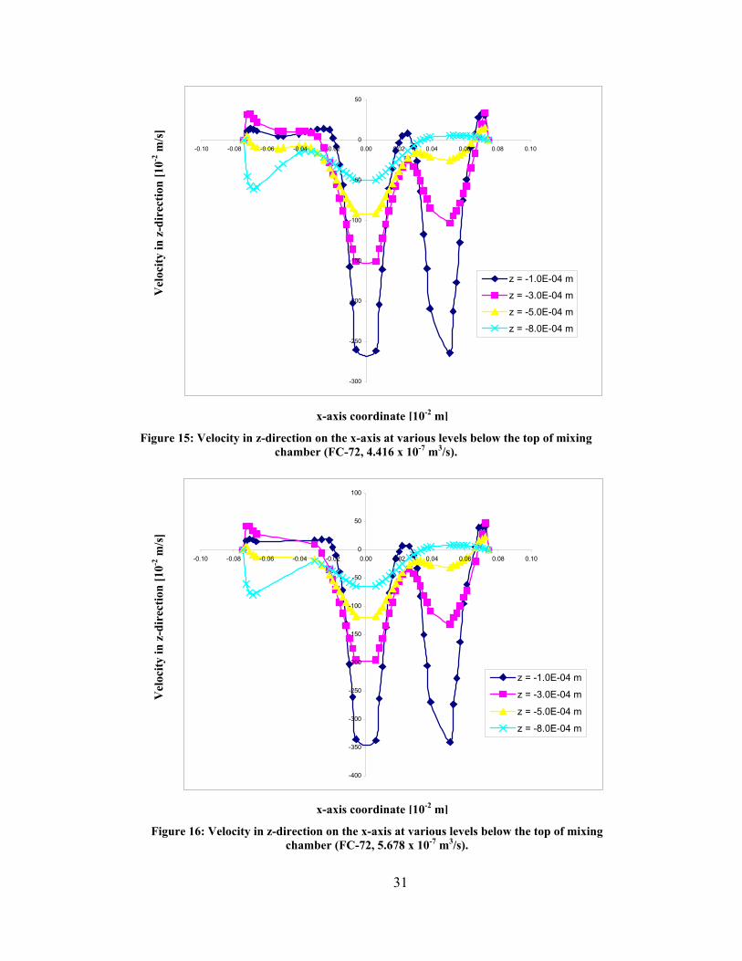
31
-300
-250
-200
-150
-100
-50
0
50
-0.10 -0.08 -0.06 -0.04 -0.02 0.00 0.02 0.04 0.06 0.08 0.10
z = -1.0E-04 m
z = -3.0E-04 m
z = -5.0E-04 m
z = -8.0E-04 m
-400
-350
-300
-250
-200
-150
-100
-50
0
50
100
-0.10 -0.08 -0.06 -0.04 -0.02 0.00 0.02 0.04 0.06 0.08 0.10
z = -1.0E-04 m
z = -3.0E-04 m
z = -5.0E-04 m
z = -8.0E-04 m
x-axis coordinate [10-2 m]
Figure 15: Velocity in z-direction on the x-axis at various levels below the top of mixing chamber (FC-72, 4.416 x 10⁻⁷ m3/s).
Vel
ocity
in z
-dir
ectio
n [1
0-2 m
/s]
x-axis coordinate [10-2 m]
Figure 16: Velocity in z-direction on the x-axis at various levels below the top of mixing chamber (FC-72, 5.678 x 10⁻⁷ m3/s).
Vel
ocity
in z
-dir
ectio
n [1
0-2 m
/s]
32
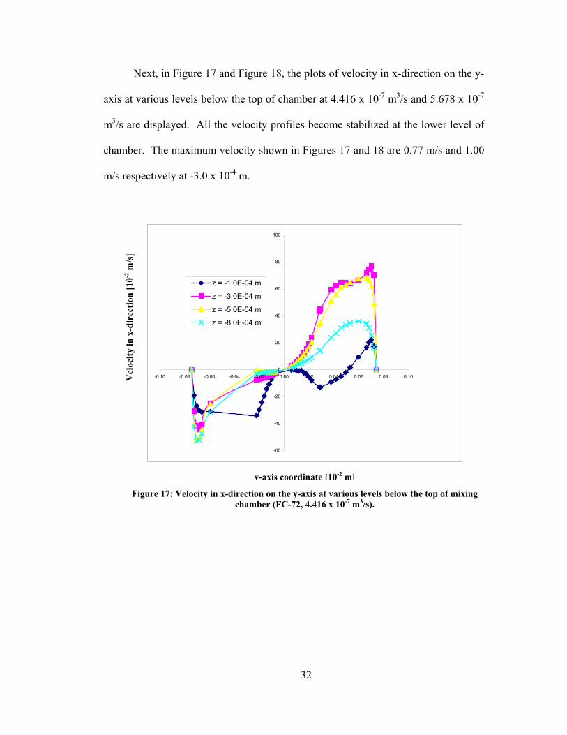
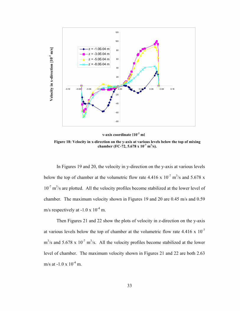
Next, in Figure 17 and Figure 18, the plots of velocity in x-direction on the y-
axis at various levels below the top of chamber at 4.416 x 10⁻⁷ m3/s and 5.678 x 10⁻⁷
m3/s are displayed. All the velocity profiles become stabilized at the lower level of
chamber. The maximum velocity shown in Figures 17 and 18 are 0.77 m/s and 1.00
m/s respectively at -3.0 x 10⁻⁴ m.
-60
-40
-20
0
20
40
60
80
100
-0.10 -0.08 -0.06 -0.04 -0.02 0.00 0.02 0.04 0.06 0.08 0.10
z = -1.0E-04 m
z = -3.0E-04 m
z = -5.0E-04 m
z = -8.0E-04 m
Figure 17: Velocity in x-direction on the y-axis at various levels below the top of mixing
chamber (FC-72, 4.416 x 10⁻⁷ m3/s).
y-axis coordinate [10-2 m]
Vel
ocity
in x
-dir
ectio
n [1
0-2 m
/s]
33
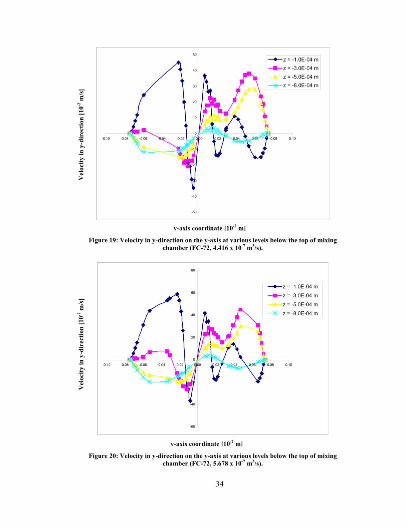
In Figures 19 and 20, the velocity in y-direction on the y-axis at various levels
below the top of chamber at the volumetric flow rate 4.416 x 10⁻⁷ m3/s and 5.678 x
10-7 m3/s are plotted. All the velocity profiles become stabilized at the lower level of
chamber. The maximum velocity shown in Figures 19 and 20 are 0.45 m/s and 0.59
m/s respectively at -1.0 x 10⁻⁴ m.
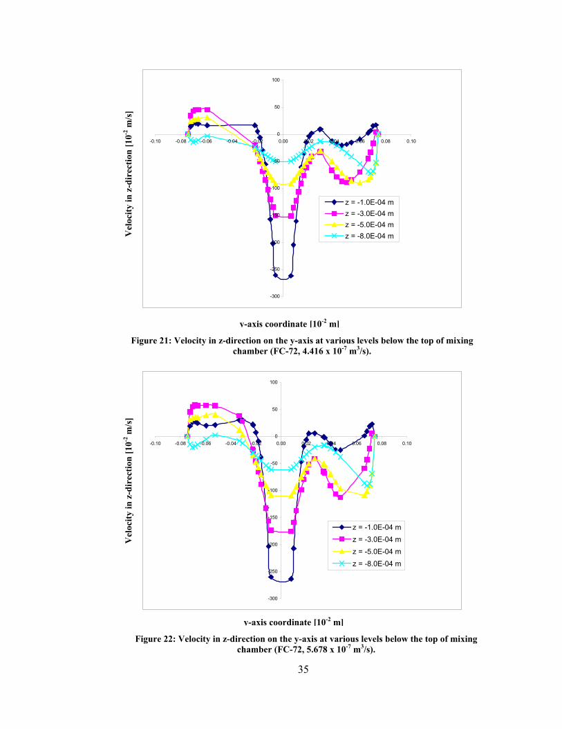
Then Figures 21 and 22 show the plots of velocity in z-direction on the y-axis
at various levels below the top of chamber at the volumetric flow rate 4.416 x 10⁻⁷
m3/s and 5.678 x 10⁻⁷ m3/s. All the velocity profiles become stabilized at the lower
level of chamber. The maximum velocity shown in Figures 21 and 22 are both 2.63
m/s at -1.0 x 10⁻⁴ m.
-80
-60
-40
-20
0
20
40
60
80
100
120
-0.10 -0.08 -0.06 -0.04 -0.02 0.00 0.02 0.04 0.06 0.08 0.10
z = -1.0E-04 mz = -3.0E-04 mz = -5.0E-04 mz = -8.0E-04 m
y-axis coordinate [10-2 m]
Figure 18: Velocity in x-direction on the y-axis at various levels below the top of mixing chamber (FC-72, 5.678 x 10⁻⁷ m3/s).
Vel
ocity
in x
-dir
ectio
n [1
0-2 m
/s]
34
-50
-40
-30
-20
-10
0
10
20
30
40
50
-0.10 -0.08 -0.06 -0.04 -0.02 0.00 0.02 0.04 0.06 0.08 0.10
z = -1.0E-04 mz = -3.0E-04 mz = -5.0E-04 mz = -8.0E-04 m
-60
-40
-20
0
20
40
60
80
-0.10 -0.08 -0.06 -0.04 -0.02 0.00 0.02 0.04 0.06 0.08 0.10
z = -1.0E-04 m
z = -3.0E-04 m
z = -5.0E-04 m
z = -8.0E-04 m
y-axis coordinate [10-2 m]
Vel
ocity
in y
-dir
ectio
n [1
0-2 m
/s]
Figure 19: Velocity in y-direction on the y-axis at various levels below the top of mixing chamber (FC-72, 4.416 x 10⁻⁷ m3/s).
y-axis coordinate [10-2 m]
Vel
ocity
in y
-dir
ectio
n [1
0-2 m
/s]
Figure 20: Velocity in y-direction on the y-axis at various levels below the top of mixing chamber (FC-72, 5.678 x 10⁻⁷ m3/s).
35
-300
-250
-200
-150
-100
-50
0
50
100
-0.10 -0.08 -0.06 -0.04 -0.02 0.00 0.02 0.04 0.06 0.08 0.10
z = -1.0E-04 mz = -3.0E-04 mz = -5.0E-04 mz = -8.0E-04 m
-300
-250
-200
-150
-100
-50
0
50
100
-0.10 -0.08 -0.06 -0.04 -0.02 0.00 0.02 0.04 0.06 0.08 0.10
z = -1.0E-04 mz = -3.0E-04 mz = -5.0E-04 mz = -8.0E-04 m
y-axis coordinate [10-2 m]
Vel
ocity
in z
-dir
ectio
n [1
0-2 m
/s]
Figure 21: Velocity in z-direction on the y-axis at various levels below the top of mixing chamber (FC-72, 4.416 x 10⁻⁷ m3/s).
y-axis coordinate [10-2 m]
Figure 22: Velocity in z-direction on the y-axis at various levels below the top of mixing chamber (FC-72, 5.678 x 10⁻⁷ m3/s).
Vel
ocity
in z
-dir
ectio
n [1
0-2 m
/s]
36
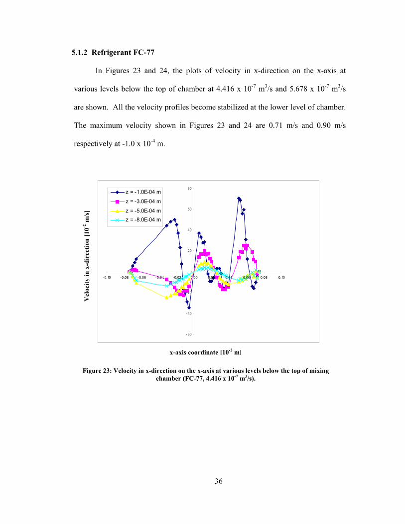
5.1.2 Refrigerant FC-77
In Figures 23 and 24, the plots of velocity in x-direction on the x-axis at
various levels below the top of chamber at 4.416 x 10⁻⁷ m3/s and 5.678 x 10⁻⁷ m3/s
are shown. All the velocity profiles become stabilized at the lower level of chamber.
The maximum velocity shown in Figures 23 and 24 are 0.71 m/s and 0.90 m/s
respectively at -1.0 x 10⁻⁴ m.
-60
-40
-20
0
20
40
60
80
-0.10 -0.08 -0.06 -0.04 -0.02 0.00 0.02 0.04 0.06 0.08 0.10
z = -1.0E-04 m
z = -3.0E-04 m
z = -5.0E-04 mz = -8.0E-04 m
Figure 23: Velocity in x-direction on the x-axis at various levels below the top of mixingchamber (FC-77, 4.416 x 10⁻⁷ m3/s).
x-axis coordinate [10-2 m]
Vel
ocity
in x
-dir
ectio
n [1
0-2 m
/s]
37
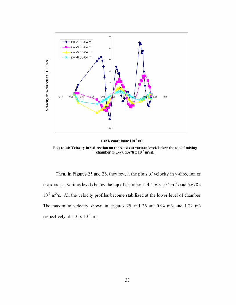
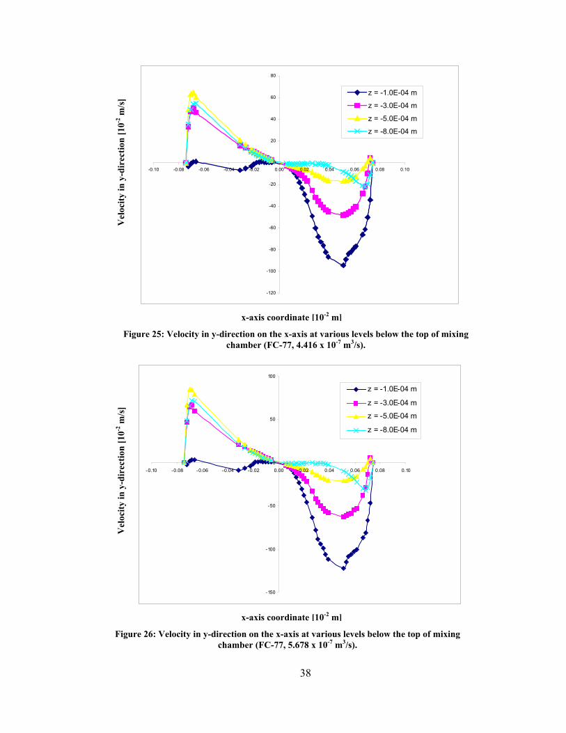
Then, in Figures 25 and 26, they reveal the plots of velocity in y-direction on
the x-axis at various levels below the top of chamber at 4.416 x 10⁻⁷ m3/s and 5.678 x
10-7 m3/s. All the velocity profiles become stabilized at the lower level of chamber.
The maximum velocity shown in Figures 25 and 26 are 0.94 m/s and 1.22 m/s
respectively at -1.0 x 10⁻⁴ m.
-60
-40
-20
0
20
40
60
80
100
-0.10 -0.08 -0.06 -0.04 -0.02 0.00 0.02 0.04 0.06 0.08 0.10
z = -1.0E-04 mz = -3.0E-04 mz = -5.0E-04 mz = -8.0E-04 m
Figure 24: Velocity in x-direction on the x-axis at various levels below the top of mixing chamber (FC-77, 5.678 x 10⁻⁷ m3/s).
x-axis coordinate [10-2 m]
Vel
ocity
in x
-dir
ectio
n [1
0-2 m
/s]
38
-120
-100
-80
-60
-40
-20
0
20
40
60
80
-0.10 -0.08 -0.06 -0.04 -0.02 0.00 0.02 0.04 0.06 0.08 0.10
z = -1.0E-04 m
z = -3.0E-04 m
z = -5.0E-04 m
z = -8.0E-04 m
-150
-100
-50
0
50
100
-0.10 -0.08 -0.06 -0.04 -0.02 0.00 0.02 0.04 0.06 0.08 0.10
z = -1.0E-04 m
z = -3.0E-04 m
z = -5.0E-04 m
z = -8.0E-04 m
x-axis coordinate [10-2 m]
Figure 25: Velocity in y-direction on the x-axis at various levels below the top of mixing chamber (FC-77, 4.416 x 10⁻⁷ m3/s).
Vel
ocity
in y
-dir
ectio
n [1
0-2 m
/s]
x-axis coordinate [10-2 m]
Figure 26: Velocity in y-direction on the x-axis at various levels below the top of mixing chamber (FC-77, 5.678 x 10⁻⁷ m3/s).
Vel
ocity
in y
-dir
ectio
n [1
0-2 m
/s]
39
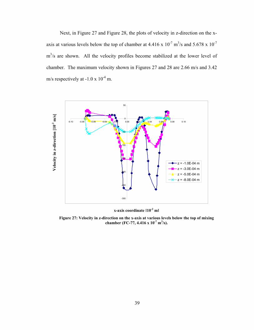
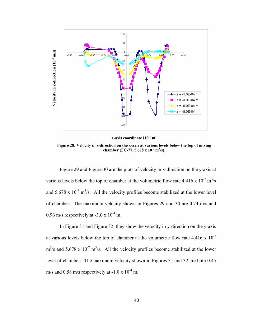
Next, in Figure 27 and Figure 28, the plots of velocity in z-direction on the x-
axis at various levels below the top of chamber at 4.416 x 10⁻⁷ m3/s and 5.678 x 10⁻⁷
m3/s are shown. All the velocity profiles become stabilized at the lower level of
chamber. The maximum velocity shown in Figures 27 and 28 are 2.66 m/s and 3.42
m/s respectively at -1.0 x 10⁻⁴ m.
-300
-250
-200
-150
-100
-50
0
50
-0.10 -0.08 -0.06 -0.04 -0.02 0.00 0.02 0.04 0.06 0.08 0.10
z = -1.0E-04 mz = -3.0E-04 mz = -5.0E-04 mz = -8.0E-04 m
Figure 27: Velocity in z-direction on the x-axis at various levels below the top of mixing
chamber (FC-77, 4.416 x 10⁻⁷ m3/s).
x-axis coordinate [10-2 m]
Vel
ocity
in z
-dir
ectio
n [1
0-2 m
/s]
40
Figure 29 and Figure 30 are the plots of velocity in x-direction on the y-axis at
various levels below the top of chamber at the volumetric flow rate 4.416 x 10⁻⁷ m3/s
and 5.678 x 10⁻⁷ m3/s. All the velocity profiles become stabilized at the lower level
of chamber. The maximum velocity shown in Figures 29 and 30 are 0.74 m/s and
0.96 m/s respectively at -3.0 x 10⁻⁴ m.
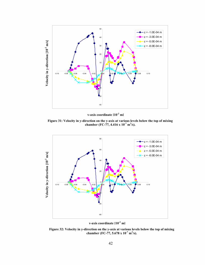
In Figure 31 and Figure 32, they show the velocity in y-direction on the y-axis
at various levels below the top of chamber at the volumetric flow rate 4.416 x 10⁻⁷
m3/s and 5.678 x 10⁻⁷ m3/s. All the velocity profiles become stabilized at the lower
level of chamber. The maximum velocity shown in Figures 31 and 32 are both 0.45
m/s and 0.58 m/s respectively at -1.0 x 10⁻⁴ m.
-400
-350
-300
-250
-200
-150
-100
-50
0
50
100
-0.10 -0.08 -0.06 -0.04 -0.02 0.00 0.02 0.04 0.06 0.08 0.10
z = -1.0E-04 m
z = -3.0E-04 m
z = -5.0E-04 m
z = -8.0E-04 m
x-axis coordinate [10-2 m]
Figure 28: Velocity in z-direction on the x-axis at various levels below the top of mixing chamber (FC-77, 5.678 x 10⁻⁷ m3/s).
Vel
ocity
in z
-dir
ectio
n [1
0-2 m
/s]

41
-60
-40
-20
0
20
40
60
80
-0.10 -0.08 -0.06 -0.04 -0.02 0.00 0.02 0.04 0.06 0.08 0.10
z = -1.0E-04 m
z = -3.0E-04 m
z = -5.0E-04 m
z = -8.0E-04 m
-80
-60
-40
-20
0
20
40
60
80
100
120
-0.10 -0.08 -0.06 -0.04 -0.02 0.00 0.02 0.04 0.06 0.08 0.10
z = -1.0E-04 m
z = -3.0E-04 m
z = -5.0E-04 m
z = -8.0E-04 m
y-axis coordinate [10-2 m]
Vel
ocity
in x
-dir
ectio
n [1
0-2 m
/s]
Figure 29: Velocity in x-direction on the y-axis at various levels below the top of mixing chamber (FC-77, 4.416 x 10⁻⁷ m3/s).
y-axis coordinate [10-2 m]
Vel
ocity
in x
-dir
ectio
n [1
0-2 m
/s]
Figure 30: Velocity in x-direction on the y-axis at various levels below the top of mixing chamber (FC-77, 5.678 x 10⁻⁷ m3/s).
42
-40
-30
-20
-10
0
10
20
30
40
50
-0.10 -0.08 -0.06 -0.04 -0.02 0.00 0.02 0.04 0.06 0.08 0.10
z = -1.0E-04 m
z = -3.0E-04 m
z = -5.0E-04 m
z = -8.0E-04 m
-60
-40
-20
0
20
40
60
80
-0.10 -0.08 -0.06 -0.04 -0.02 0.00 0.02 0.04 0.06 0.08 0.10
z = -1.0E-04 m
z = -3.0E-04 m
z = -5.0E-04 m
z = -8.0E-04 m
y-axis coordinate [10-2 m]
Vel
ocity
in y
-dir
ectio
n [1
0-2 m
/s]
Figure 31: Velocity in y-direction on the y-axis at various levels below the top of mixing chamber (FC-77, 4.416 x 10⁻⁷ m3/s).
y-axis coordinate [10-2 m]
Figure 32: Velocity in y-direction on the y-axis at various levels below the top of mixing chamber (FC-77, 5.678 x 10⁻⁷ m3/s).
Vel
ocity
in y
-dir
ectio
n [1
0-2 m
/s]
43
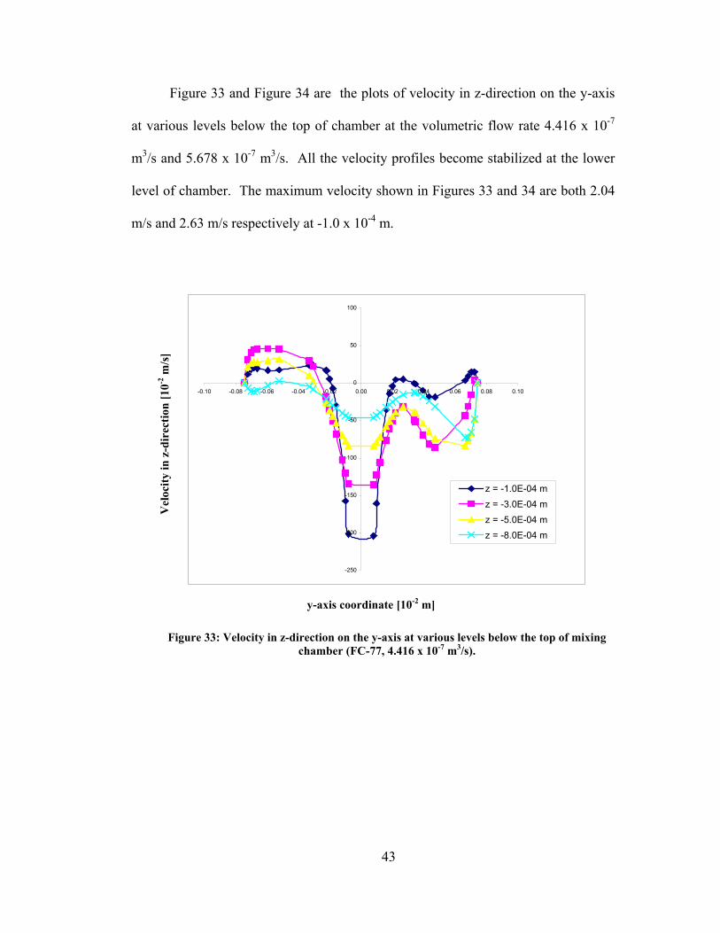
Figure 33 and Figure 34 are the plots of velocity in z-direction on the y-axis
at various levels below the top of chamber at the volumetric flow rate 4.416 x 10⁻⁷
m3/s and 5.678 x 10⁻⁷ m3/s. All the velocity profiles become stabilized at the lower
level of chamber. The maximum velocity shown in Figures 33 and 34 are both 2.04
m/s and 2.63 m/s respectively at -1.0 x 10⁻⁴ m.
-250
-200
-150
-100
-50
0
50
100
-0.10 -0.08 -0.06 -0.04 -0.02 0.00 0.02 0.04 0.06 0.08 0.10
z = -1.0E-04 mz = -3.0E-04 mz = -5.0E-04 mz = -8.0E-04 m
y-axis coordinate [10-2 m]
Vel
ocity
in z
-dir
ectio
n [1
0-2 m
/s]
Figure 33: Velocity in z-direction on the y-axis at various levels below the top of mixing chamber (FC-77, 4.416 x 10⁻⁷ m3/s).
44
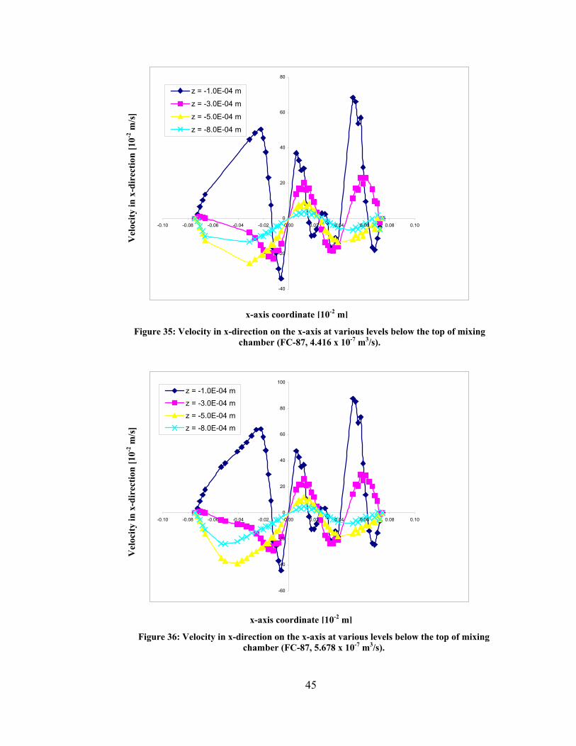
5.1.3 Refrigerant FC-87
In Figures 35 and 36, they reveal the plots of velocity in x-direction on the x-
axis at various levels below the top of chamber at 4.416 x 10⁻⁷ m3/s and 5.678 x 10⁻⁷
m3/s. All the velocity profiles become stabilized at the lower level of chamber. The
maximum velocity shown in Figures 35 and 36 are 0.68 m/s and 0.88 m/s
respectively at -1.0 x 10⁻⁴ m.
-300
-250
-200
-150
-100
-50
0
50
100
-0.10 -0.08 -0.06 -0.04 -0.02 0.00 0.02 0.04 0.06 0.08 0.10
z = -1.0E-04 m
z = -3.0E-04 m
z = -5.0E-04 m
z = -8.0E-04 m
y-axis coordinate [10-2 m]
Figure 34: Velocity in z-direction on the y-axis at various levels below the top of mixing chamber (FC-77, 5.678 x 10⁻⁷ m3/s).
Vel
ocity
in z
-dir
ectio
n [1
0-2 m
/s]
45
-40
-20
0
20
40
60
80
-0.10 -0.08 -0.06 -0.04 -0.02 0.00 0.02 0.04 0.06 0.08 0.10
z = -1.0E-04 m
z = -3.0E-04 m
z = -5.0E-04 m
z = -8.0E-04 m
-60
-40
-20
0
20
40
60
80
100
-0.10 -0.08 -0.06 -0.04 -0.02 0.00 0.02 0.04 0.06 0.08 0.10
z = -1.0E-04 mz = -3.0E-04 mz = -5.0E-04 mz = -8.0E-04 m
x-axis coordinate [10-2 m]
Vel
ocity
in x
-dir
ectio
n [1
0-2 m
/s]
Figure 35: Velocity in x-direction on the x-axis at various levels below the top of mixing chamber (FC-87, 4.416 x 10⁻⁷ m3/s).
x-axis coordinate [10-2 m]
Figure 36: Velocity in x-direction on the x-axis at various levels below the top of mixing chamber (FC-87, 5.678 x 10⁻⁷ m3/s).
Vel
ocity
in x
-dir
ectio
n [1
0-2 m
/s]
46
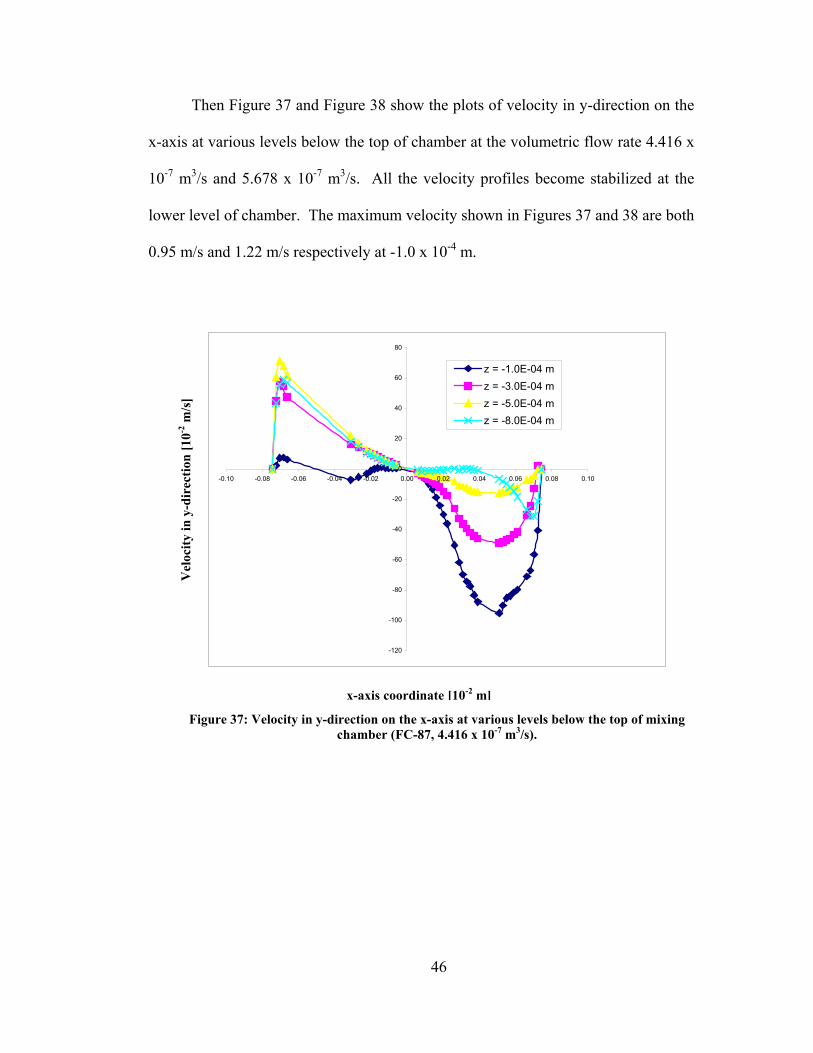
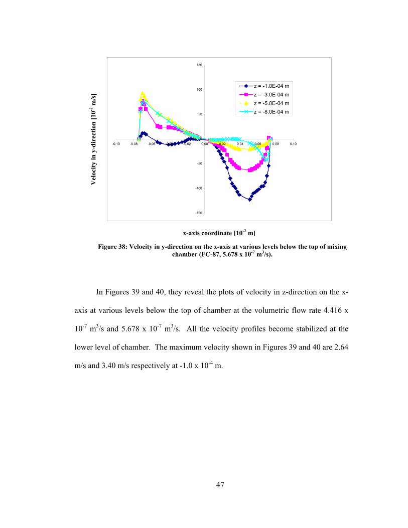
Then Figure 37 and Figure 38 show the plots of velocity in y-direction on the
x-axis at various levels below the top of chamber at the volumetric flow rate 4.416 x
10-7 m3/s and 5.678 x 10⁻⁷ m3/s. All the velocity profiles become stabilized at the
lower level of chamber. The maximum velocity shown in Figures 37 and 38 are both
0.95 m/s and 1.22 m/s respectively at -1.0 x 10⁻⁴ m.
-120
-100
-80
-60
-40
-20
0
20
40
60
80
-0.10 -0.08 -0.06 -0.04 -0.02 0.00 0.02 0.04 0.06 0.08 0.10
z = -1.0E-04 mz = -3.0E-04 mz = -5.0E-04 mz = -8.0E-04 m
x-axis coordinate [10-2 m]
Vel
ocity
in y
-dir
ectio
n [1
0-2 m
/s]
Figure 37: Velocity in y-direction on the x-axis at various levels below the top of mixing chamber (FC-87, 4.416 x 10⁻⁷ m3/s).
47
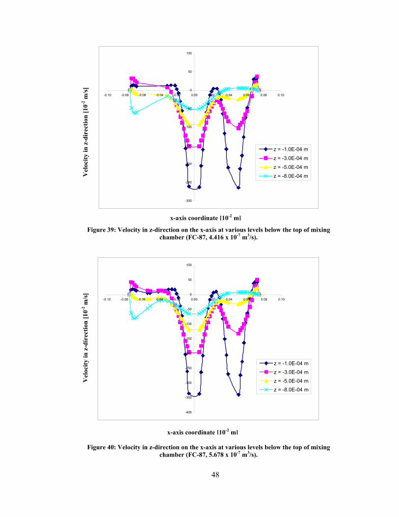
In Figures 39 and 40, they reveal the plots of velocity in z-direction on the x-
axis at various levels below the top of chamber at the volumetric flow rate 4.416 x
10-7 m3/s and 5.678 x 10⁻⁷ m3/s. All the velocity profiles become stabilized at the
lower level of chamber. The maximum velocity shown in Figures 39 and 40 are 2.64
m/s and 3.40 m/s respectively at -1.0 x 10⁻⁴ m.
-150
-100
-50
0
50
100
150
-0.10 -0.08 -0.06 -0.04 -0.02 0.00 0.02 0.04 0.06 0.08 0.10
z = -1.0E-04 mz = -3.0E-04 mz = -5.0E-04 mz = -8.0E-04 m
x-axis coordinate [10-2 m]
Figure 38: Velocity in y-direction on the x-axis at various levels below the top of mixing chamber (FC-87, 5.678 x 10⁻⁷ m3/s).
Vel
ocity
in y
-dir
ectio
n [1
0-2 m
/s]
48
-300
-250
-200
-150
-100
-50
0
50
100
-0.10 -0.08 -0.06 -0.04 -0.02 0.00 0.02 0.04 0.06 0.08 0.10
z = -1.0E-04 m
z = -3.0E-04 m
z = -5.0E-04 m
z = -8.0E-04 m
-400
-350
-300
-250
-200
-150
-100
-50
0
50
100
-0.10 -0.08 -0.06 -0.04 -0.02 0.00 0.02 0.04 0.06 0.08 0.10
z = -1.0E-04 m
z = -3.0E-04 m
z = -5.0E-04 m
z = -8.0E-04 m
x-axis coordinate [10-2 m]
Vel
ocity
in z
-dir
ectio
n [1
0-2 m
/s]
Figure 39: Velocity in z-direction on the x-axis at various levels below the top of mixing chamber (FC-87, 4.416 x 10⁻⁷ m3/s).
x-axis coordinate [10-2 m]
Vel
ocity
in z
-dir
ectio
n [1
0-2 m
/s]
Figure 40: Velocity in z-direction on the x-axis at various levels below the top of mixing chamber (FC-87, 5.678 x 10⁻⁷ m3/s).
49
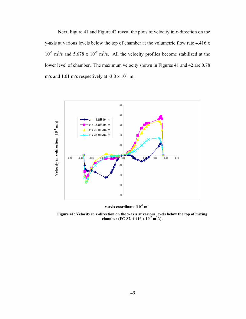
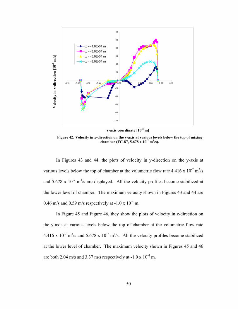
Next, Figure 41 and Figure 42 reveal the plots of velocity in x-direction on the
y-axis at various levels below the top of chamber at the volumetric flow rate 4.416 x
10-7 m3/s and 5.678 x 10⁻⁷ m3/s. All the velocity profiles become stabilized at the
lower level of chamber. The maximum velocity shown in Figures 41 and 42 are 0.78
m/s and 1.01 m/s respectively at -3.0 x 10⁻⁴ m.
-80
-60
-40
-20
0
20
40
60
80
100
-0.10 -0.08 -0.06 -0.04 -0.02 0.00 0.02 0.04 0.06 0.08 0.10
z = -1.0E-04 mz = -3.0E-04 mz = -5.0E-04 mz = -8.0E-04 m
y-axis coordinate [10-2 m]
Vel
ocity
in x
-dir
ectio
n [1
0-2 m
/s]
Figure 41: Velocity in x-direction on the y-axis at various levels below the top of mixing chamber (FC-87, 4.416 x 10⁻⁷ m3/s).
50
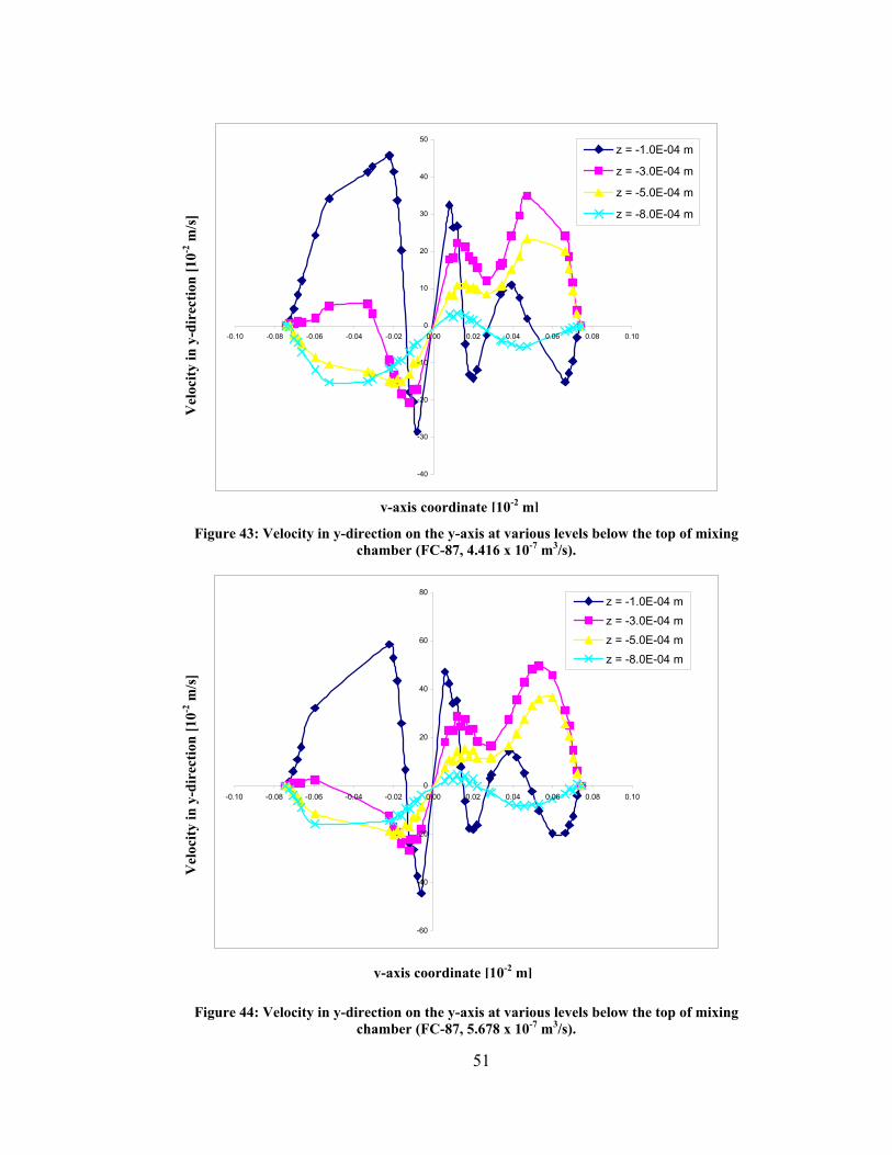
In Figures 43 and 44, the plots of velocity in y-direction on the y-axis at
various levels below the top of chamber at the volumetric flow rate 4.416 x 10⁻⁷ m3/s
and 5.678 x 10⁻⁷ m3/s are displayed. All the velocity profiles become stabilized at
the lower level of chamber. The maximum velocity shown in Figures 43 and 44 are
0.46 m/s and 0.59 m/s respectively at -1.0 x 10⁻⁴ m.
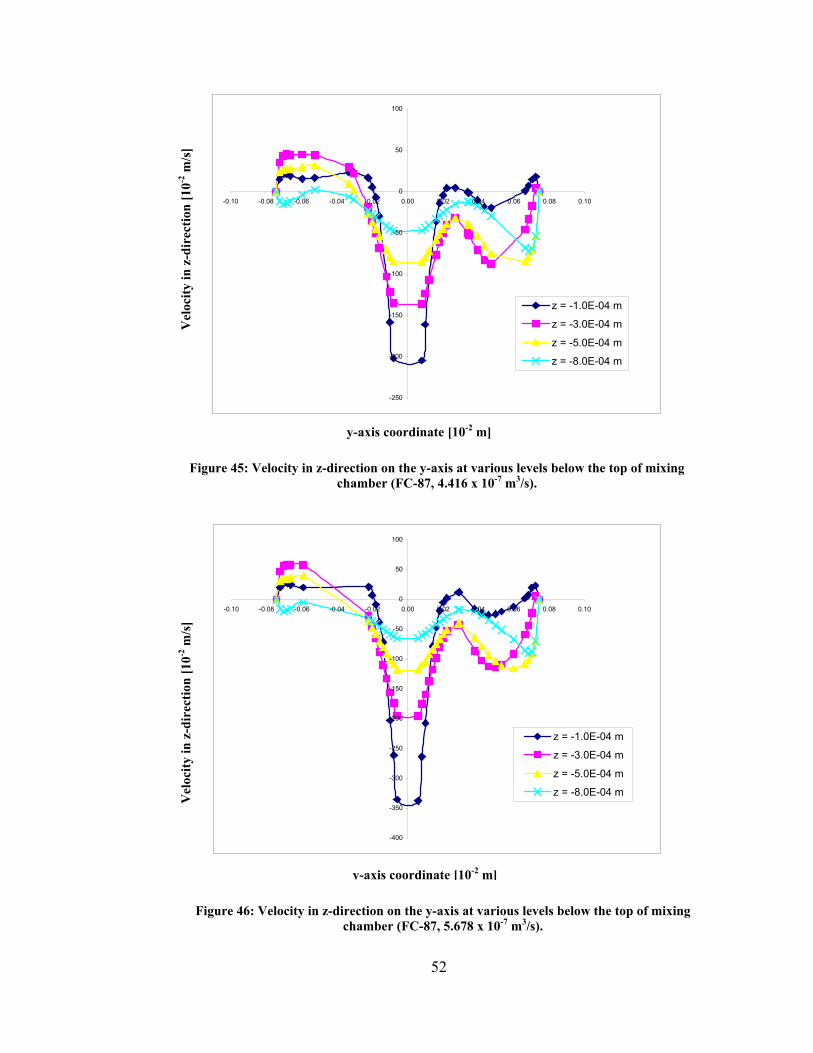
In Figure 45 and Figure 46, they show the plots of velocity in z-direction on
the y-axis at various levels below the top of chamber at the volumetric flow rate
4.416 x 10⁻⁷ m3/s and 5.678 x 10⁻⁷ m3/s. All the velocity profiles become stabilized
at the lower level of chamber. The maximum velocity shown in Figures 45 and 46
are both 2.04 m/s and 3.37 m/s respectively at -1.0 x 10⁻⁴ m.
-100
-80
-60
-40
-20
0
20
40
60
80
100
120
-0.10 -0.08 -0.06 -0.04 -0.02 0.00 0.02 0.04 0.06 0.08 0.10
z = -1.0E-04 mz = -3.0E-04 mz = -5.0E-04 mz = -8.0E-04 m
y-axis coordinate [10-2 m]
Figure 42: Velocity in x-direction on the y-axis at various levels below the top of mixing chamber (FC-87, 5.678 x 10⁻⁷ m3/s).
Vel
ocity
in x
-dir
ectio
n [1
0-2 m
/s]
51
-40
-30
-20
-10
0
10
20
30
40
50
-0.10 -0.08 -0.06 -0.04 -0.02 0.00 0.02 0.04 0.06 0.08 0.10
z = -1.0E-04 m
z = -3.0E-04 m
z = -5.0E-04 m
z = -8.0E-04 m
-60
-40
-20
0
20
40
60
80
-0.10 -0.08 -0.06 -0.04 -0.02 0.00 0.02 0.04 0.06 0.08 0.10
z = -1.0E-04 mz = -3.0E-04 mz = -5.0E-04 mz = -8.0E-04 m
y-axis coordinate [10-2 m]
Vel
ocity
in y
-dir
ectio
n [1
0-2 m
/s]
Figure 43: Velocity in y-direction on the y-axis at various levels below the top of mixing chamber (FC-87, 4.416 x 10⁻⁷ m3/s).
y-axis coordinate [10-2 m]
Vel
ocity
in y
-dir
ectio
n [1
0-2 m
/s]
Figure 44: Velocity in y-direction on the y-axis at various levels below the top of mixing chamber (FC-87, 5.678 x 10⁻⁷ m3/s).
52
-250
-200
-150
-100
-50
0
50
100
-0.10 -0.08 -0.06 -0.04 -0.02 0.00 0.02 0.04 0.06 0.08 0.10
z = -1.0E-04 m
z = -3.0E-04 m
z = -5.0E-04 m
z = -8.0E-04 m
-400
-350
-300
-250
-200
-150
-100
-50
0
50
100
-0.10 -0.08 -0.06 -0.04 -0.02 0.00 0.02 0.04 0.06 0.08 0.10
z = -1.0E-04 m
z = -3.0E-04 m
z = -5.0E-04 m
z = -8.0E-04 m
y-axis coordinate [10-2 m]
Vel
ocity
in z
-dir
ectio
n [1
0-2 m
/s]
Figure 45: Velocity in z-direction on the y-axis at various levels below the top of mixing chamber (FC-87, 4.416 x 10⁻⁷ m3/s).
y-axis coordinate [10-2 m]
Figure 46: Velocity in z-direction on the y-axis at various levels below the top of mixing chamber (FC-87, 5.678 x 10⁻⁷ m3/s).
Vel
ocity
in z
-dir
ectio
n [1
0-2 m
/s]
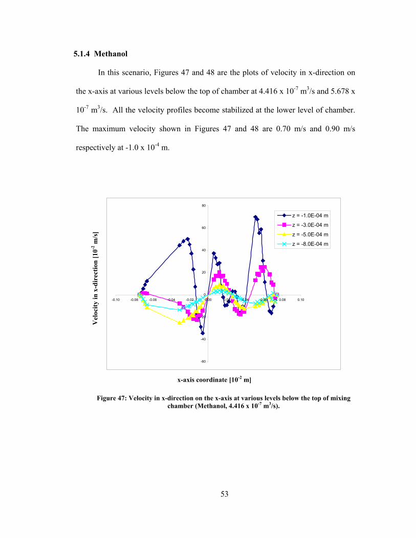
53
5.1.4 Methanol
In this scenario, Figures 47 and 48 are the plots of velocity in x-direction on
the x-axis at various levels below the top of chamber at 4.416 x 10⁻⁷ m3/s and 5.678 x
10-7 m3/s. All the velocity profiles become stabilized at the lower level of chamber.
The maximum velocity shown in Figures 47 and 48 are 0.70 m/s and 0.90 m/s
respectively at -1.0 x 10⁻⁴ m.
-60
-40
-20
0
20
40
60
80
-0.10 -0.08 -0.06 -0.04 -0.02 0.00 0.02 0.04 0.06 0.08 0.10
z = -1.0E-04 m
z = -3.0E-04 m
z = -5.0E-04 m
z = -8.0E-04 m
x-axis coordinate [10-2 m]
Vel
ocity
in x
-dir
ectio
n [1
0-2 m
/s]
Figure 47: Velocity in x-direction on the x-axis at various levels below the top of mixing chamber (Methanol, 4.416 x 10⁻⁷ m3/s).
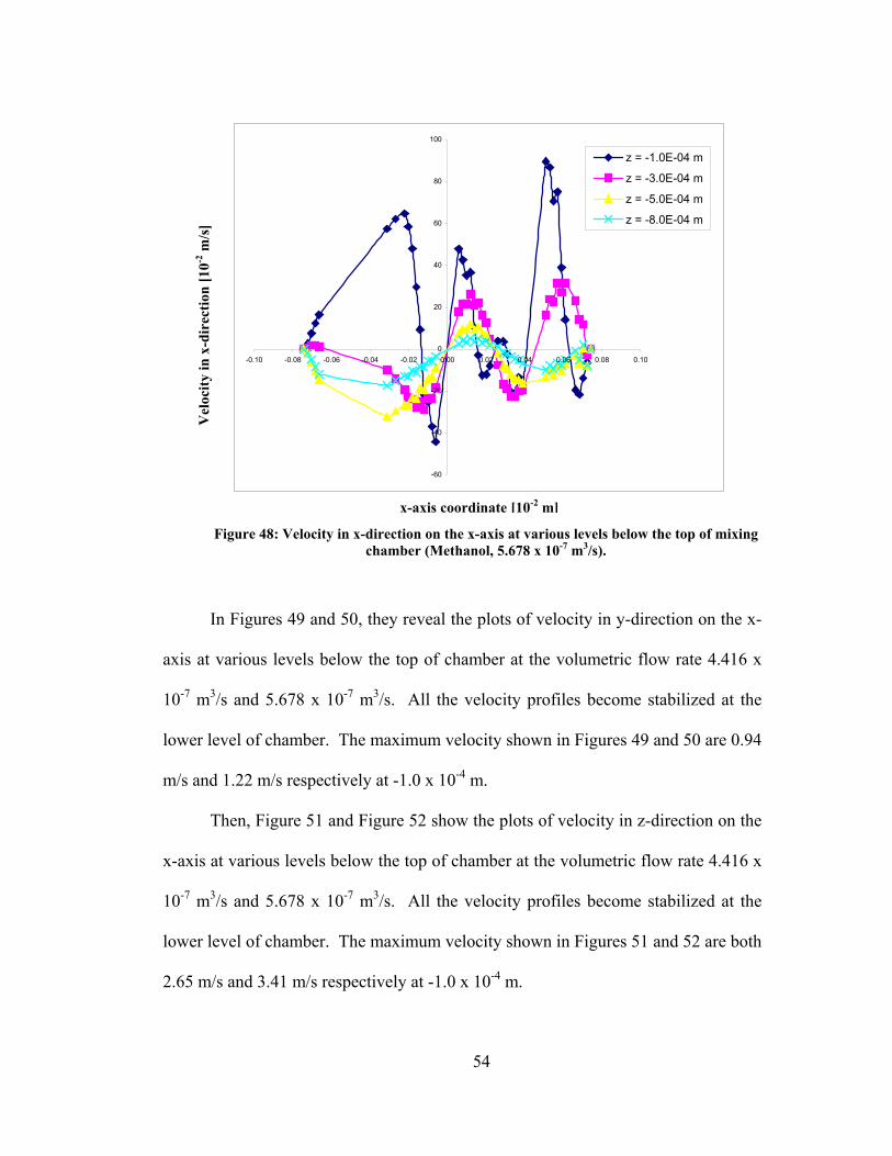
54
In Figures 49 and 50, they reveal the plots of velocity in y-direction on the x-
axis at various levels below the top of chamber at the volumetric flow rate 4.416 x
10-7 m3/s and 5.678 x 10⁻⁷ m3/s. All the velocity profiles become stabilized at the
lower level of chamber. The maximum velocity shown in Figures 49 and 50 are 0.94
m/s and 1.22 m/s respectively at -1.0 x 10⁻⁴ m.
Then, Figure 51 and Figure 52 show the plots of velocity in z-direction on the
x-axis at various levels below the top of chamber at the volumetric flow rate 4.416 x
10-7 m3/s and 5.678 x 10⁻⁷ m3/s. All the velocity profiles become stabilized at the
lower level of chamber. The maximum velocity shown in Figures 51 and 52 are both
2.65 m/s and 3.41 m/s respectively at -1.0 x 10⁻⁴ m.
-60
-40
-20
0
20
40
60
80
100
-0.10 -0.08 -0.06 -0.04 -0.02 0.00 0.02 0.04 0.06 0.08 0.10
z = -1.0E-04 m
z = -3.0E-04 m
z = -5.0E-04 m
z = -8.0E-04 m
x-axis coordinate [10-2 m]
Figure 48: Velocity in x-direction on the x-axis at various levels below the top of mixing chamber (Methanol, 5.678 x 10⁻⁷ m3/s).
Vel
ocity
in x
-dir
ectio
n [1
0-2 m
/s]

55
-120
-100
-80
-60
-40
-20
0
20
40
60
80
-0.10 -0.08 -0.06 -0.04 -0.02 0.00 0.02 0.04 0.06 0.08 0.10
z = -1.0E-04 m
z = -3.0E-04 m
z = -5.0E-04 m
z = -8.0E-04 m
-150
-100
-50
0
50
100
-0.10 -0.08 -0.06 -0.04 -0.02 0.00 0.02 0.04 0.06 0.08 0.10
z = -1.0E-04 mz = -3.0E-04 mz = -5.0E-04 mz = -8.0E-04 m
x-axis coordinate [10-2 m]
Vel
ocity
in y
-dir
ectio
n [1
0-2 m
/s]
Figure 49: Velocity in y-direction on the x-axis at various levels below the top of mixing chamber (Methanol, 4.416 x 10⁻⁷ m3/s).
x-axis coordinate [10-2 m]
Vel
ocity
in y
-dir
ectio
n [1
0-2 m
/s]
Figure 50: Velocity in y-direction on the x-axis at various levels below the top of mixing chamber (Methanol, 5.678 x 10⁻⁷ m3/s).
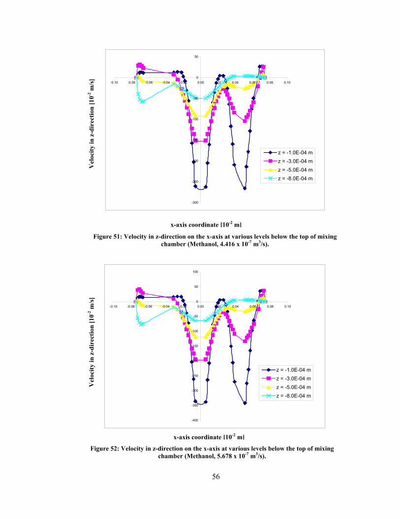
56
-300
-250
-200
-150
-100
-50
0
50
-0.10 -0.08 -0.06 -0.04 -0.02 0.00 0.02 0.04 0.06 0.08 0.10
z = -1.0E-04 mz = -3.0E-04 mz = -5.0E-04 mz = -8.0E-04 m
-400
-350
-300
-250
-200
-150
-100
-50
0
50
100
-0.10 -0.08 -0.06 -0.04 -0.02 0.00 0.02 0.04 0.06 0.08 0.10
z = -1.0E-04 mz = -3.0E-04 mz = -5.0E-04 mz = -8.0E-04 m
x-axis coordinate [10-2 m]
Vel
ocity
in z
-dir
ectio
n [1
0-2 m
/s]
Figure 51: Velocity in z-direction on the x-axis at various levels below the top of mixing chamber (Methanol, 4.416 x 10⁻⁷ m3/s).
x-axis coordinate [10-2 m]
Figure 52: Velocity in z-direction on the x-axis at various levels below the top of mixing chamber (Methanol, 5.678 x 10⁻⁷ m3/s).
Vel
ocity
in z
-dir
ectio
n [1
0-2 m
/s]

57
In Figures 53 and 54, they display the plots of velocity in x-direction on the y-
axis at various levels below the top of chamber at 4.416 x 10⁻⁷ m3/s and 5.678 x 10⁻⁷
m3/s. All the velocity profiles become stabilized at the lower level of chamber. The
maximum velocity shown in Figures 53 and 54 are 0.74 m/s and 0.97 m/s
respectively at -3.0 x 10⁻⁴ m.
-60
-40
-20
0
20
40
60
80
100
-0.10 -0.08 -0.06 -0.04 -0.02 0.00 0.02 0.04 0.06 0.08 0.10
z = -1.0E-04 mz = -3.0E-04 mz = -5.0E-04 mz = -8.0E-04 m
y-axis coordinate [10-2 m]
Vel
ocity
in x
-dir
ectio
n [1
0-2 m
/s]
Figure 53: Velocity in x-direction on the y-axis at various levels below the top of mixing chamber (Methanol, 4.416 x 10⁻⁷ m3/s).
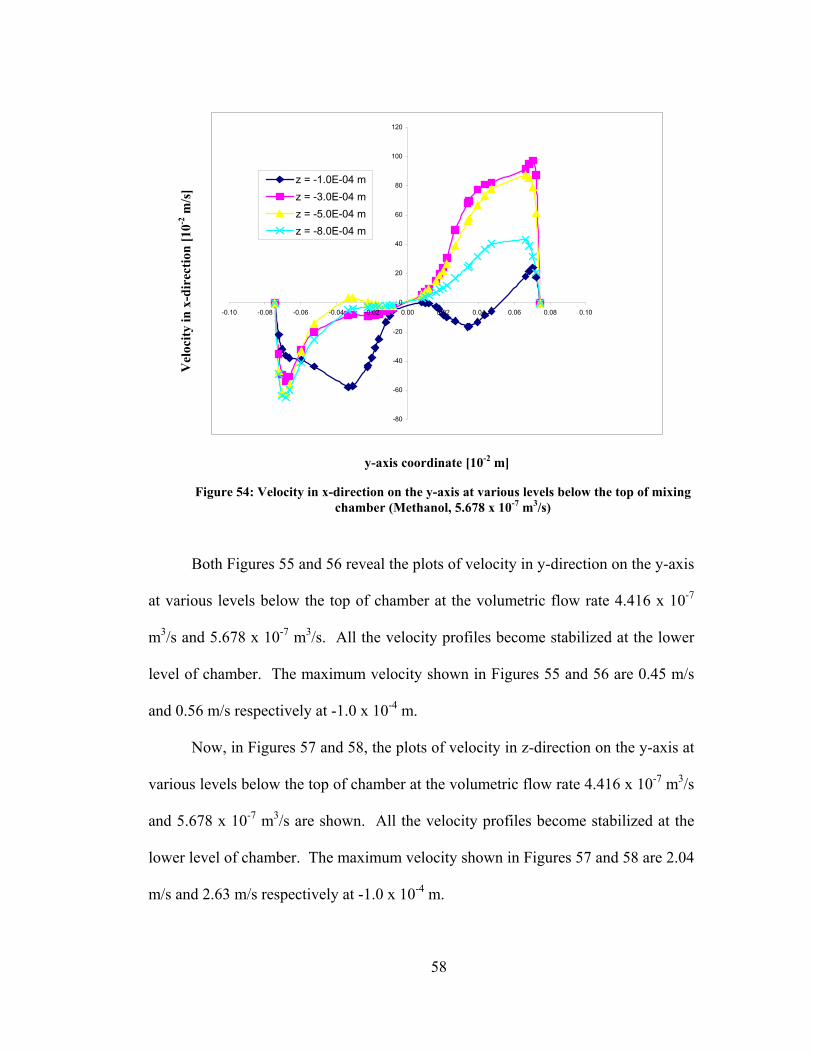
58
Both Figures 55 and 56 reveal the plots of velocity in y-direction on the y-axis
at various levels below the top of chamber at the volumetric flow rate 4.416 x 10⁻⁷
m3/s and 5.678 x 10⁻⁷ m3/s. All the velocity profiles become stabilized at the lower
level of chamber. The maximum velocity shown in Figures 55 and 56 are 0.45 m/s
and 0.56 m/s respectively at -1.0 x 10⁻⁴ m.
Now, in Figures 57 and 58, the plots of velocity in z-direction on the y-axis at
various levels below the top of chamber at the volumetric flow rate 4.416 x 10⁻⁷ m3/s
and 5.678 x 10⁻⁷ m3/s are shown. All the velocity profiles become stabilized at the
lower level of chamber. The maximum velocity shown in Figures 57 and 58 are 2.04
m/s and 2.63 m/s respectively at -1.0 x 10⁻⁴ m.
-80
-60
-40
-20
0
20
40
60
80
100
120
-0.10 -0.08 -0.06 -0.04 -0.02 0.00 0.02 0.04 0.06 0.08 0.10
z = -1.0E-04 mz = -3.0E-04 mz = -5.0E-04 mz = -8.0E-04 m
y-axis coordinate [10-2 m]
Figure 54: Velocity in x-direction on the y-axis at various levels below the top of mixing chamber (Methanol, 5.678 x 10⁻⁷ m3/s)
Vel
ocity
in x
-dir
ectio
n [1
0-2 m
/s]
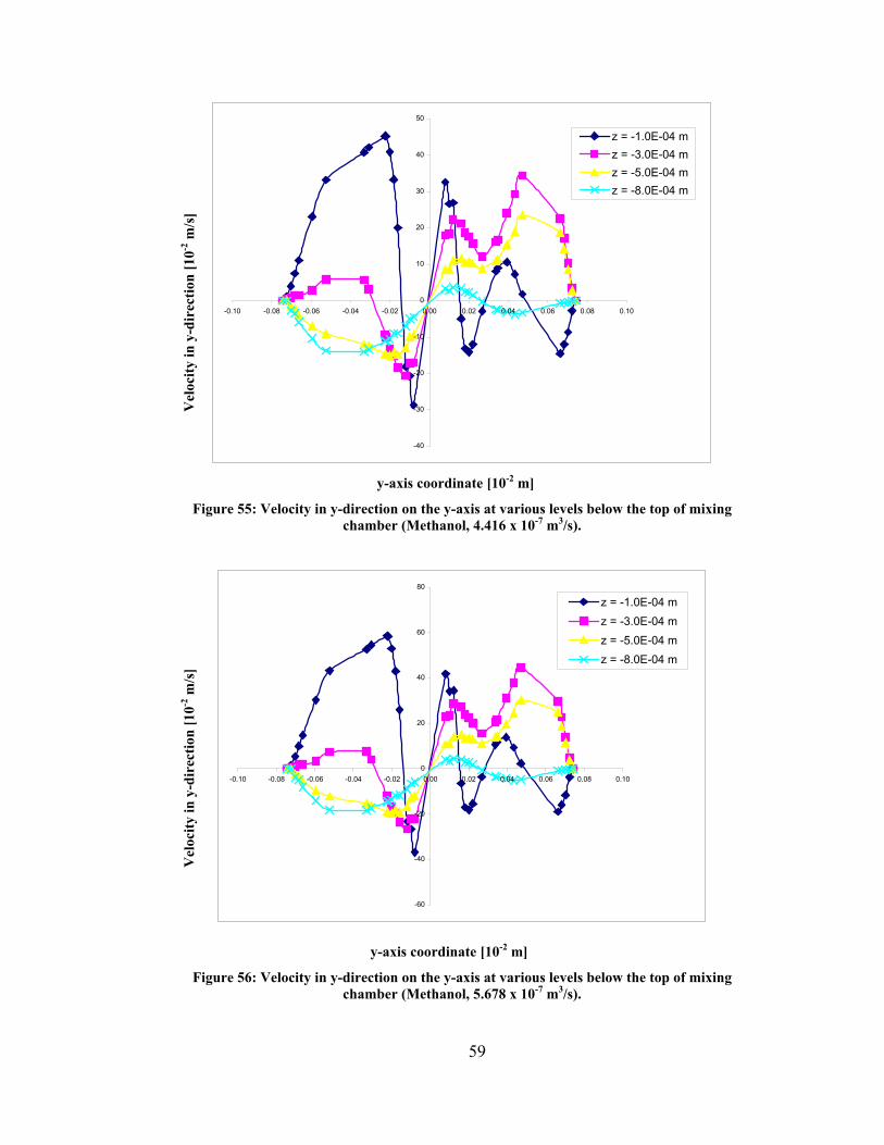
59
-40
-30
-20
-10
0
10
20
30
40
50
-0.10 -0.08 -0.06 -0.04 -0.02 0.00 0.02 0.04 0.06 0.08 0.10
z = -1.0E-04 mz = -3.0E-04 mz = -5.0E-04 mz = -8.0E-04 m
-60
-40
-20
0
20
40
60
80
-0.10 -0.08 -0.06 -0.04 -0.02 0.00 0.02 0.04 0.06 0.08 0.10
z = -1.0E-04 mz = -3.0E-04 mz = -5.0E-04 mz = -8.0E-04 m
y-axis coordinate [10-2 m]
Vel
ocity
in y
-dir
ectio
n [1
0-2 m
/s]
Figure 55: Velocity in y-direction on the y-axis at various levels below the top of mixing chamber (Methanol, 4.416 x 10⁻⁷ m3/s).
y-axis coordinate [10-2 m]
Vel
ocity
in y
-dir
ectio
n [1
0-2 m
/s]
Figure 56: Velocity in y-direction on the y-axis at various levels below the top of mixing chamber (Methanol, 5.678 x 10⁻⁷ m3/s).
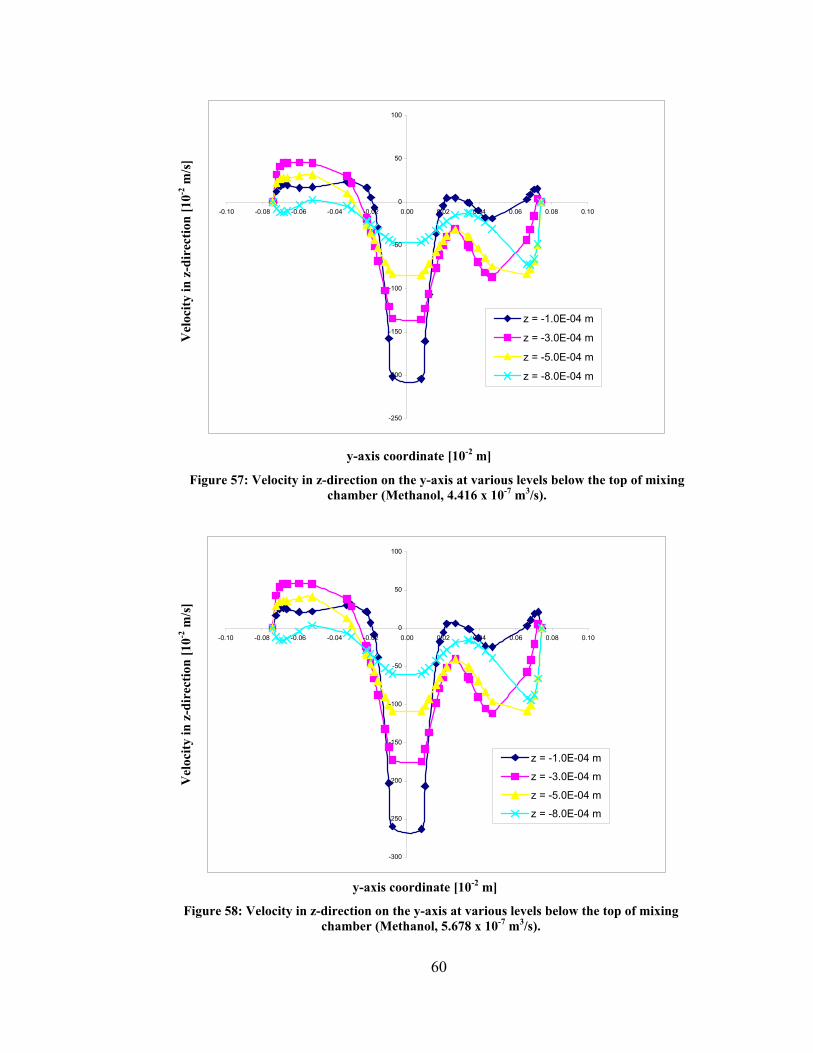
60
-250
-200
-150
-100
-50
0
50
100
-0.10 -0.08 -0.06 -0.04 -0.02 0.00 0.02 0.04 0.06 0.08 0.10
z = -1.0E-04 m
z = -3.0E-04 m
z = -5.0E-04 m
z = -8.0E-04 m
-300
-250
-200
-150
-100
-50
0
50
100
-0.10 -0.08 -0.06 -0.04 -0.02 0.00 0.02 0.04 0.06 0.08 0.10
z = -1.0E-04 m
z = -3.0E-04 m
z = -5.0E-04 m
z = -8.0E-04 m
y-axis coordinate [10-2 m]
Vel
ocity
in z
-dir
ectio
n [1
0-2 m
/s]
Figure 57: Velocity in z-direction on the y-axis at various levels below the top of mixing chamber (Methanol, 4.416 x 10⁻⁷ m3/s).
y-axis coordinate [10-2 m]
Figure 58: Velocity in z-direction on the y-axis at various levels below the top of mixing chamber (Methanol, 5.678 x 10⁻⁷ m3/s).
Vel
ocity
in z
-dir
ectio
n [1
0-2 m
/s]
61
Based on the results of the 3D simulation, the flow patterns for each working
fluid at different flow rates were nearly identical. First, the velocity of fluid flowing
inside the inlet tubes was much faster than its velocity in the chamber. Besides, the
pressure decreased gradually from the inlets to the chamber bottom. Obviously, the
velocities in x, y, and z directions increased when the volumetric flow rate increased.
Next, the velocity profiles in each direction became stabilized as the fluid eventually
approached the bottom of chamber. Also, there was a flow spinning in a clockwise
motion shown in Figure 59 to Figure 66.
After that, the velocities in x, y, z-directions were obtained, and they were all
transformed into radial, circumferential, and axial velocities. Since the transformed
velocities in each direction were not the same, they were then averaged and became
the average velocities in cylindrical system for the axi-symmetrical nozzle
simulations.
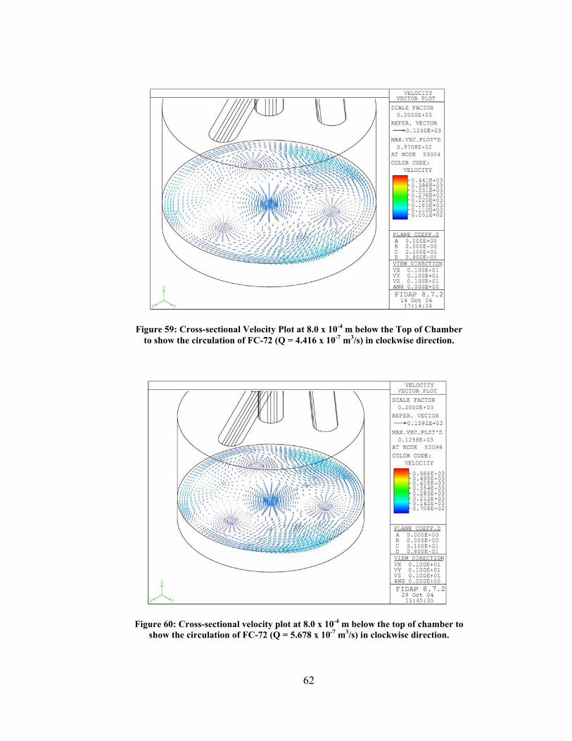
62
Figure 59: Cross-sectional Velocity Plot at 8.0 x 10⁻⁴ m below the Top of Chamber
to show the circulation of FC-72 (Q = 4.416 x 10⁻⁷ m3/s) in clockwise direction.
Figure 60: Cross-sectional velocity plot at 8.0 x 10⁻⁴ m below the top of chamber to
show the circulation of FC-72 (Q = 5.678 x 10⁻⁷ m3/s) in clockwise direction.

63
Figure 61: Cross-sectional velocity plot at 8.0 x 10⁻⁴ m below the top of chamber to show the circulation of FC-77 (Q = 4.416 x 10⁻⁷ m3/s) in clockwise direction.
Figure 62: Cross-sectional velocity plot at 8.0 x 10⁻⁴ m below the top of chamber to show the circulation of FC-77 (Q = 5.678 x 10⁻⁷ m3/s) in clockwise direction.

64
Figure 63: Cross-sectional velocity plot at 8.0 x 10⁻⁴ m below the top of chamber to show the circulation of FC-87 (Q = 4.416 x 10⁻⁷ m3/s) in clockwise direction.
Figure 64: Cross-sectional velocity plot at 8.0 x 10⁻⁴ m below the top of chamber to show the circulation of FC-87 (Q = 5.678 x 10⁻⁷ m3/s) in clockwise direction.
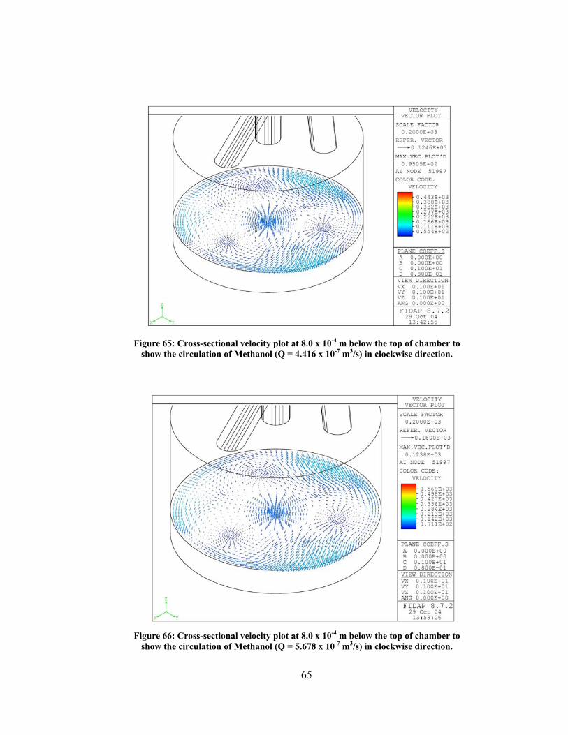
65
Figure 65: Cross-sectional velocity plot at 8.0 x 10⁻⁴ m below the top of chamber to show the circulation of Methanol (Q = 4.416 x 10⁻⁷ m3/s) in clockwise direction.
Figure 66: Cross-sectional velocity plot at 8.0 x 10⁻⁴ m below the top of chamber to show the circulation of Methanol (Q = 5.678 x 10⁻⁷ m3/s) in clockwise direction.
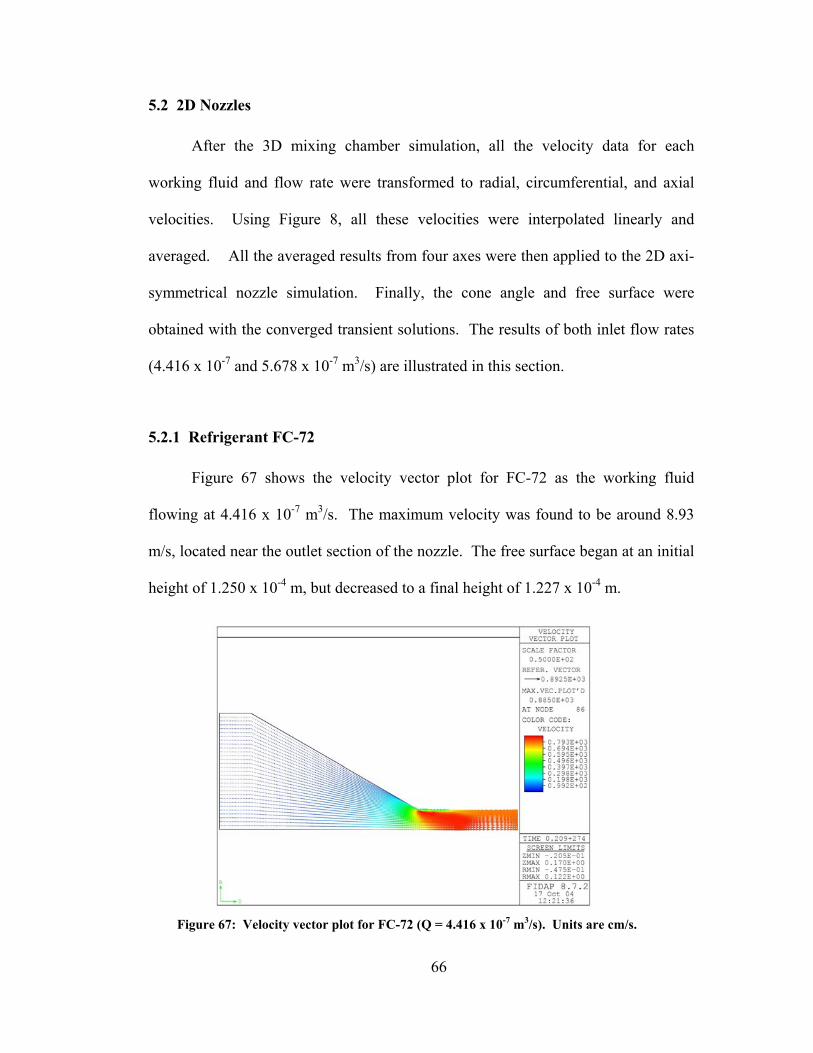
66
5.2 2D Nozzles
After the 3D mixing chamber simulation, all the velocity data for each
working fluid and flow rate were transformed to radial, circumferential, and axial
velocities. Using Figure 8, all these velocities were interpolated linearly and
averaged. All the averaged results from four axes were then applied to the 2D axi-
symmetrical nozzle simulation. Finally, the cone angle and free surface were
obtained with the converged transient solutions. The results of both inlet flow rates
(4.416 x 10⁻⁷ and 5.678 x 10⁻⁷ m3/s) are illustrated in this section.
5.2.1 Refrigerant FC-72
Figure 67 shows the velocity vector plot for FC-72 as the working fluid
flowing at 4.416 x 10⁻⁷ m3/s. The maximum velocity was found to be around 8.93
m/s, located near the outlet section of the nozzle. The free surface began at an initial
height of 1.250 x 10⁻⁴ m, but decreased to a final height of 1.227 x 10⁻⁴ m.
Figure 67: Velocity vector plot for FC-72 (Q = 4.416 x 10⁻⁷ m3/s). Units are cm/s.

67
Figure 68 and 69 show the pressure and streamline contour plots, respectively.
The maximum pressure within the nozzle was found to be 7.17 x 10⁴ Pa, while the
minimum pressure was -2.18 x 10⁴ Pa. The inlet-to-outlet pressure drop was
calculated to be about 7.20 x 10⁴ Pa. The streamline contour plot shows that most of
the fluid entering the outer slot flows along the nozzle wall toward the outlet, while
some of that fluid initially flowed toward the center of the nozzle. The fluid entering
closed to the center of nozzle flows slightly outward in the radial direction as it
moved toward the outlet.
Figure 68: Pressure contour plot for FC-72 (Q = 4.416 x 10⁻⁷ m3/s). Units are gm/cm s2
(x101 Pa).
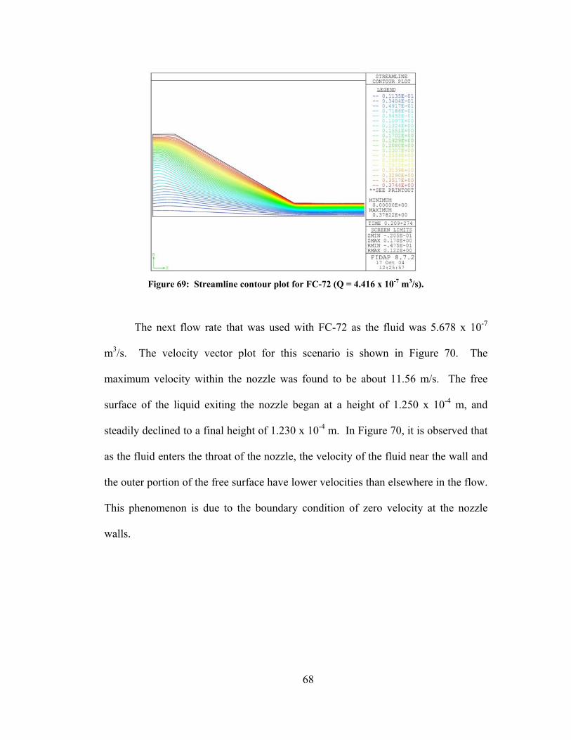
68
Figure 69: Streamline contour plot for FC-72 (Q = 4.416 x 10⁻⁷ m3/s).
The next flow rate that was used with FC-72 as the fluid was 5.678 x 10⁻⁷
m3/s. The velocity vector plot for this scenario is shown in Figure 70. The
maximum velocity within the nozzle was found to be about 11.56 m/s. The free
surface of the liquid exiting the nozzle began at a height of 1.250 x 10⁻⁴ m, and
steadily declined to a final height of 1.230 x 10⁻⁴ m. In Figure 70, it is observed that
as the fluid enters the throat of the nozzle, the velocity of the fluid near the wall and
the outer portion of the free surface have lower velocities than elsewhere in the flow.
This phenomenon is due to the boundary condition of zero velocity at the nozzle
walls.
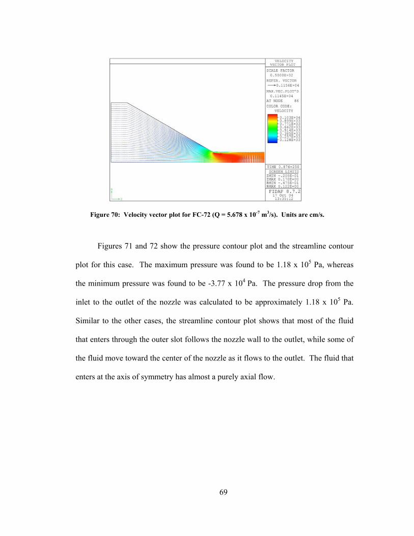
69
Figure 70: Velocity vector plot for FC-72 (Q = 5.678 x 10⁻⁷ m3/s). Units are cm/s.
Figures 71 and 72 show the pressure contour plot and the streamline contour
plot for this case. The maximum pressure was found to be 1.18 x 10⁵ Pa, whereas
the minimum pressure was found to be -3.77 x 10⁴ Pa. The pressure drop from the
inlet to the outlet of the nozzle was calculated to be approximately 1.18 x 10⁵ Pa.
Similar to the other cases, the streamline contour plot shows that most of the fluid
that enters through the outer slot follows the nozzle wall to the outlet, while some of
the fluid move toward the center of the nozzle as it flows to the outlet. The fluid that
enters at the axis of symmetry has almost a purely axial flow.

70
Figure 71: Pressure contour plot for FC-72 (Q = 5.678 x 10⁻⁷ m3/s). Units are gm/cm s2
(x101 Pa).
Figure 72: Streamline contour plot for FC-72 (Q = 5.678 x 10⁻⁷ m3/s).
Figure 73 and Figure 74 depict the profile of the free surface obtained when
the working fluid was FC-72. It was noted that the inlet flow rate had little effect on
the height of the free surface; however, 5.678 x 10⁻⁷ m3/s produced a slightly greater
height.
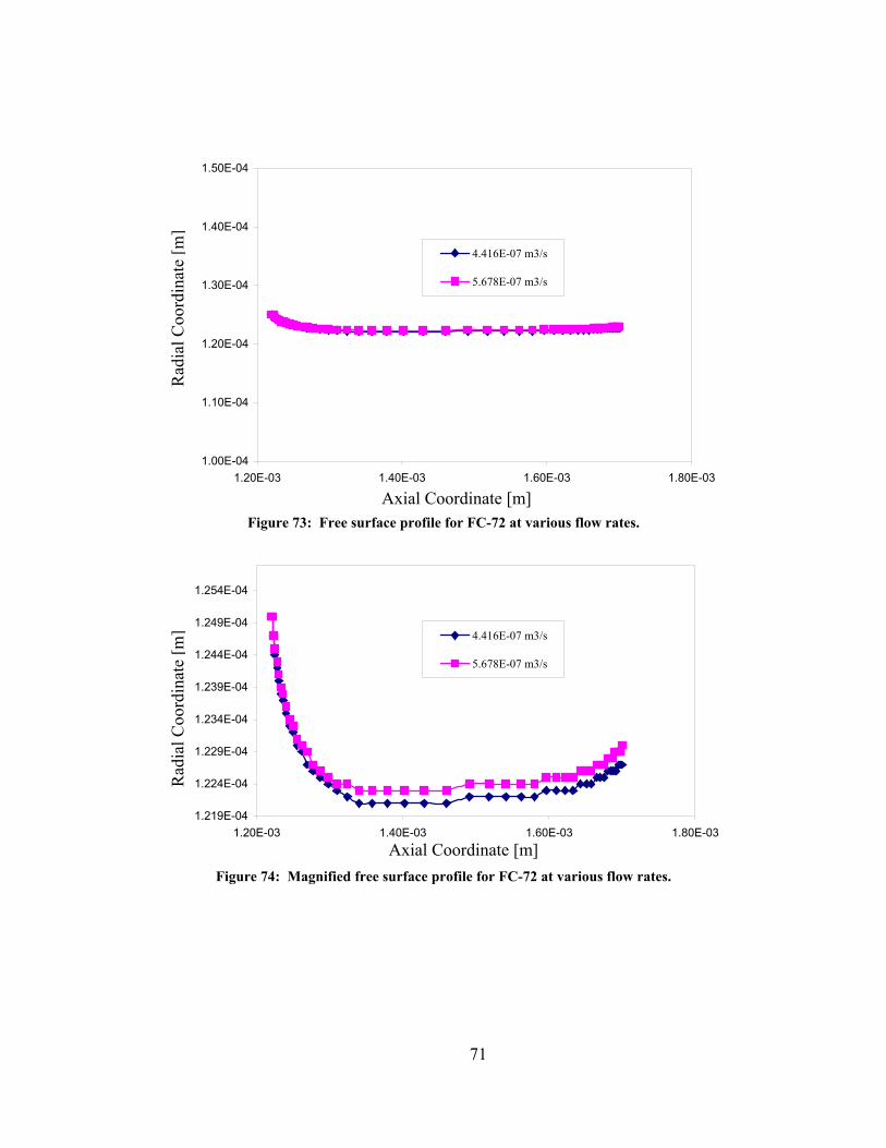
71
1.00E-04
1.10E-04
1.20E-04
1.30E-04
1.40E-04
1.50E-04
1.20E-03 1.40E-03 1.60E-03 1.80E-03
4.416E-07 m3/s
5.678E-07 m3/s
Figure 73: Free surface profile for FC-72 at various flow rates.
1.219E-04
1.224E-04
1.229E-04
1.234E-04
1.239E-04
1.244E-04
1.249E-04
1.254E-04
1.20E-03 1.40E-03 1.60E-03 1.80E-03
4.416E-07 m3/s
5.678E-07 m3/s
Figure 74: Magnified free surface profile for FC-72 at various flow rates.
Axial Coordinate [m]
Rad
ial C
oord
inat
e [m
]
Axial Coordinate [m]
Rad
ial C
oord
inat
e [m
]
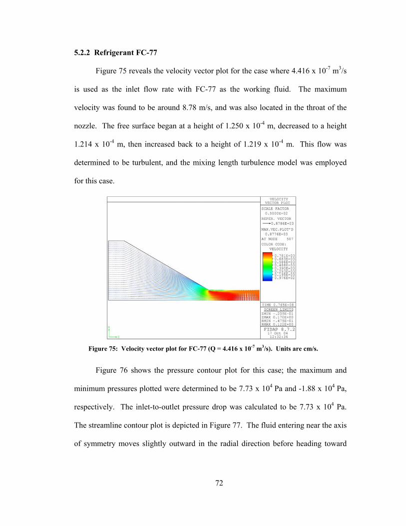
72
5.2.2 Refrigerant FC-77
Figure 75 reveals the velocity vector plot for the case where 4.416 x 10⁻⁷ m3/s
is used as the inlet flow rate with FC-77 as the working fluid. The maximum
velocity was found to be around 8.78 m/s, and was also located in the throat of the
nozzle. The free surface began at a height of 1.250 x 10⁻⁴ m, decreased to a height
1.214 x 10⁻⁴ m, then increased back to a height of 1.219 x 10⁻⁴ m. This flow was
determined to be turbulent, and the mixing length turbulence model was employed
for this case.
Figure 75: Velocity vector plot for FC-77 (Q = 4.416 x 10⁻⁷ m3/s). Units are cm/s.
Figure 76 shows the pressure contour plot for this case; the maximum and
minimum pressures plotted were determined to be 7.73 x 10⁴ Pa and -1.88 x 10⁴ Pa,
respectively. The inlet-to-outlet pressure drop was calculated to be 7.73 x 10⁴ Pa.
The streamline contour plot is depicted in Figure 77. The fluid entering near the axis
of symmetry moves slightly outward in the radial direction before heading toward

73
the outlet because the circumferential velocity increases from the center to the wall at
the nozzle inlet section.
Figure 76: Pressure contour plot for FC-77 (Q = 4.416 x 10⁻⁷ m3/s). Units are gm/cm s2
(x101 Pa).
Figure 77: Streamline contour plot for FC-77 (Q = 4.416 x 10⁻⁷ m3/s).
The velocity vector plot for FC-77 traveling at 5.678 x 10⁻⁷ m3/s is shown in
Figure 78. This was also found to be turbulent, and again, the mixing length
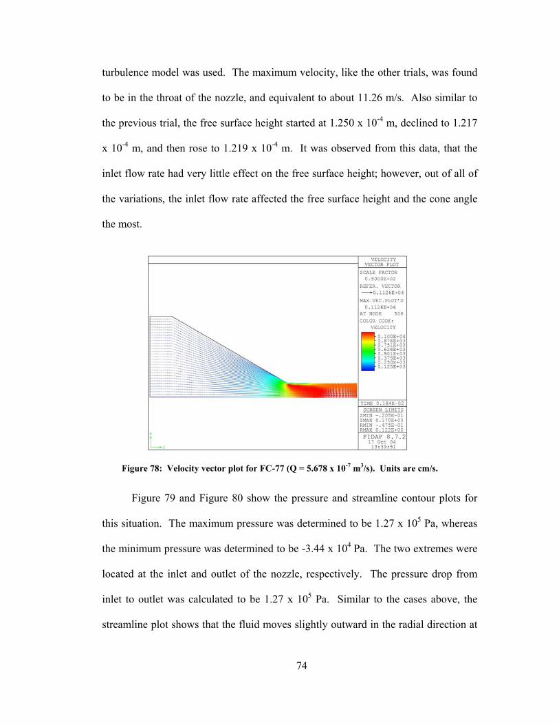
74
turbulence model was used. The maximum velocity, like the other trials, was found
to be in the throat of the nozzle, and equivalent to about 11.26 m/s. Also similar to
the previous trial, the free surface height started at 1.250 x 10⁻⁴ m, declined to 1.217
x 10-4 m, and then rose to 1.219 x 10⁻⁴ m. It was observed from this data, that the
inlet flow rate had very little effect on the free surface height; however, out of all of
the variations, the inlet flow rate affected the free surface height and the cone angle
the most.
Figure 78: Velocity vector plot for FC-77 (Q = 5.678 x 10⁻⁷ m3/s). Units are cm/s.
Figure 79 and Figure 80 show the pressure and streamline contour plots for
this situation. The maximum pressure was determined to be 1.27 x 10⁵ Pa, whereas
the minimum pressure was determined to be -3.44 x 10⁴ Pa. The two extremes were
located at the inlet and outlet of the nozzle, respectively. The pressure drop from
inlet to outlet was calculated to be 1.27 x 10⁵ Pa. Similar to the cases above, the
streamline plot shows that the fluid moves slightly outward in the radial direction at
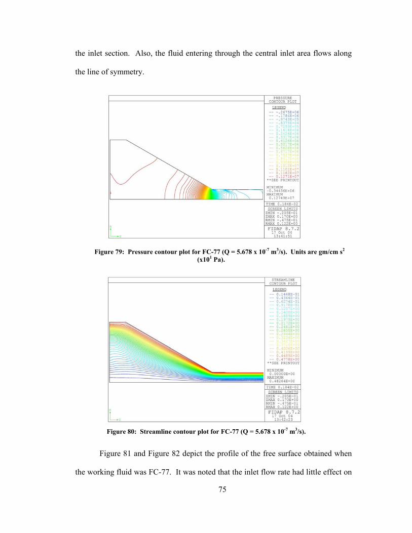
75
the inlet section. Also, the fluid entering through the central inlet area flows along
the line of symmetry.
Figure 79: Pressure contour plot for FC-77 (Q = 5.678 x 10⁻⁷ m3/s). Units are gm/cm s2
(x101 Pa).
Figure 80: Streamline contour plot for FC-77 (Q = 5.678 x 10⁻⁷ m3/s).
Figure 81 and Figure 82 depict the profile of the free surface obtained when
the working fluid was FC-77. It was noted that the inlet flow rate had little effect on
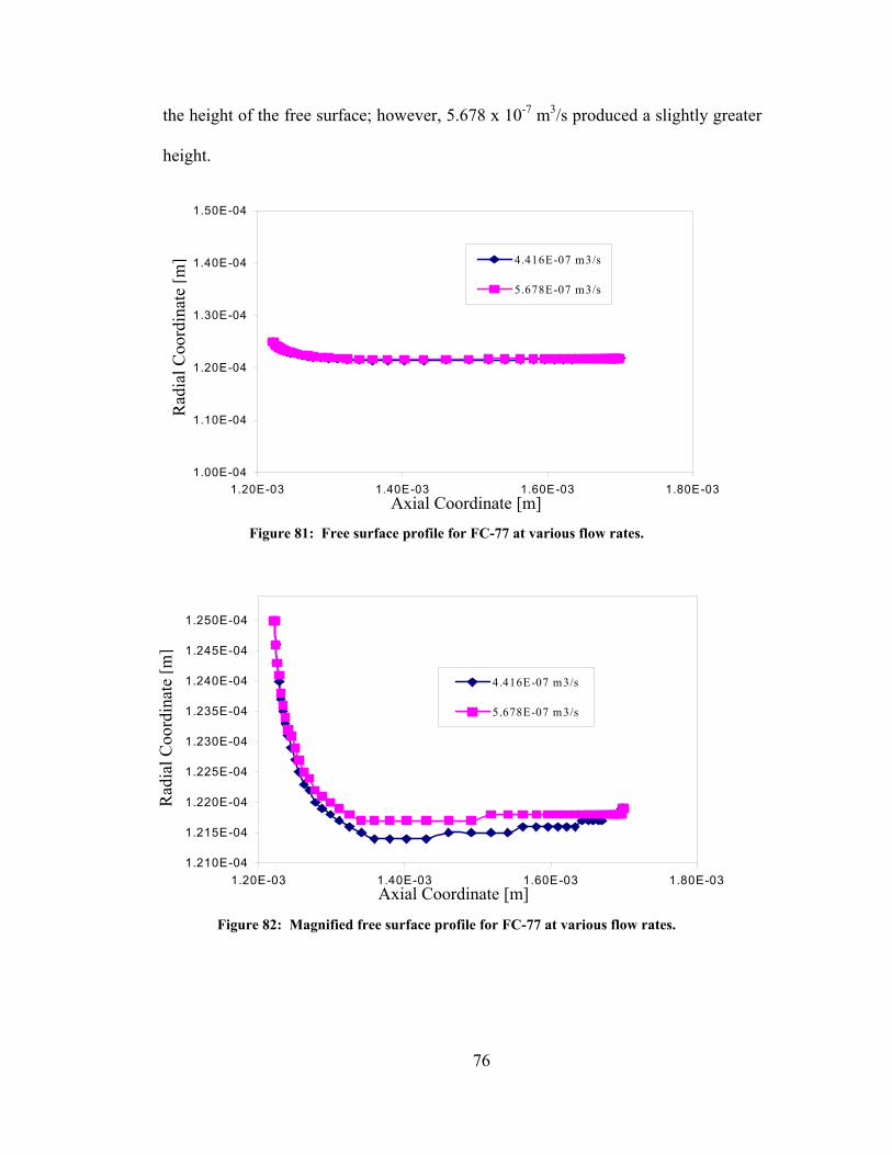
76
the height of the free surface; however, 5.678 x 10⁻⁷ m3/s produced a slightly greater
height.
1.00E-04
1.10E-04
1.20E-04
1.30E-04
1.40E-04
1.50E-04
1.20E-03 1.40E-03 1.60E-03 1.80E-03
4.416E-07 m3/s
5.678E-07 m3/s
Figure 81: Free surface profile for FC-77 at various flow rates.
1.210E-04
1.215E-04
1.220E-04
1.225E-04
1.230E-04
1.235E-04
1.240E-04
1.245E-04
1.250E-04
1.20E-03 1.40E-03 1.60E-03 1.80E-03
4.416E-07 m3/s
5.678E-07 m3/s
Figure 82: Magnified free surface profile for FC-77 at various flow rates.
Axial Coordinate [m]
Rad
ial C
oord
inat
e [m
]
Axial Coordinate [m]
Rad
ial C
oord
inat
e [m
]
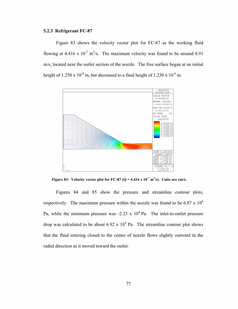
77
5.2.3 Refrigerant FC-87
Figure 83 shows the velocity vector plot for FC-87 as the working fluid
flowing at 4.416 x 10⁻⁷ m3/s. The maximum velocity was found to be around 8.91
m/s, located near the outlet section of the nozzle. The free surface began at an initial
height of 1.250 x 10⁻⁴ m, but decreased to a final height of 1.230 x 10⁻⁴ m.
Figure 83: Velocity vector plot for FC-87 (Q = 4.416 x 10⁻⁷ m3/s). Units are cm/s.
Figures 84 and 85 show the pressure and streamline contour plots,
respectively. The maximum pressure within the nozzle was found to be 6.87 x 10⁴
Pa, while the minimum pressure was -2.23 x 10⁴ Pa. The inlet-to-outlet pressure
drop was calculated to be about 6.92 x 10⁴ Pa. The streamline contour plot shows
that the fluid entering closed to the center of nozzle flows slightly outward in the
radial direction as it moved toward the outlet.

78
Figure 84: Pressure contour plot for FC-87 (Q = 4.416 x 10⁻⁷ m3/s). Units are gm/cm s2
(x101 Pa).
Figure 85: Streamline contour plot for FC-87 (Q = 4.416 x 10⁻⁷ m3/s).
The next flow rate that was used with FC-87 as the fluid was 5.678 x 10⁻⁷
m3/s. The velocity vector plot for this scenario is shown in Figure 86. The
maximum velocity within the nozzle was found to be about 11.49 m/s. The free
surface of the liquid exiting the nozzle began at a height of 1.250 x 10⁻⁴ m, steadily
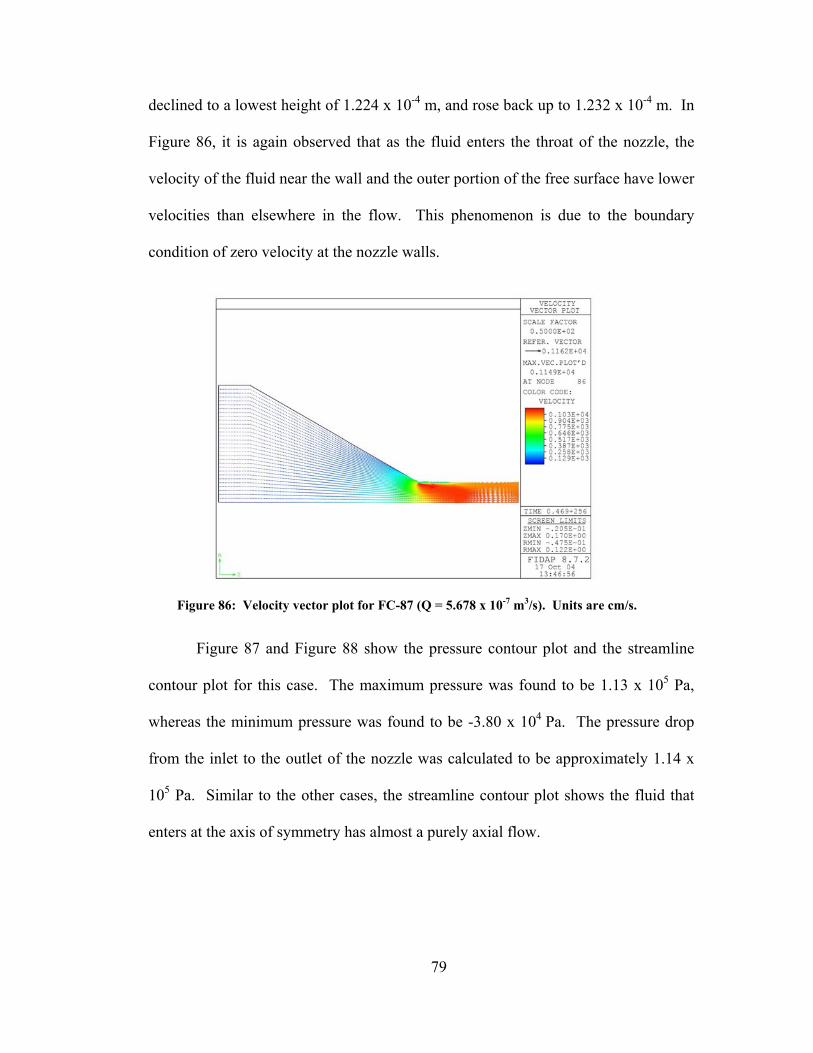
79
declined to a lowest height of 1.224 x 10⁻⁴ m, and rose back up to 1.232 x 10⁻⁴ m. In
Figure 86, it is again observed that as the fluid enters the throat of the nozzle, the
velocity of the fluid near the wall and the outer portion of the free surface have lower
velocities than elsewhere in the flow. This phenomenon is due to the boundary
condition of zero velocity at the nozzle walls.
Figure 86: Velocity vector plot for FC-87 (Q = 5.678 x 10⁻⁷ m3/s). Units are cm/s.
Figure 87 and Figure 88 show the pressure contour plot and the streamline
contour plot for this case. The maximum pressure was found to be 1.13 x 10⁵ Pa,
whereas the minimum pressure was found to be -3.80 x 10⁴ Pa. The pressure drop
from the inlet to the outlet of the nozzle was calculated to be approximately 1.14 x
105 Pa. Similar to the other cases, the streamline contour plot shows the fluid that
enters at the axis of symmetry has almost a purely axial flow.

80
Figure 87: Pressure contour plot for FC-87 (Q = 5.678 x 10⁻⁷ m3/s). Units are gm/cm s2
(x101 Pa).
Figure 88: Streamline contour plot for FC-87 (Q = 5.678 x 10⁻⁷ m3/s).
Figures 89 and 90 depict the profile of the free surface obtained when the
working fluid was FC-87. It was noted that the inlet flow rate had little effect on the
height of the free surface; however, 5.678 x 10⁻⁷ m3/s produced a slightly greater
height.
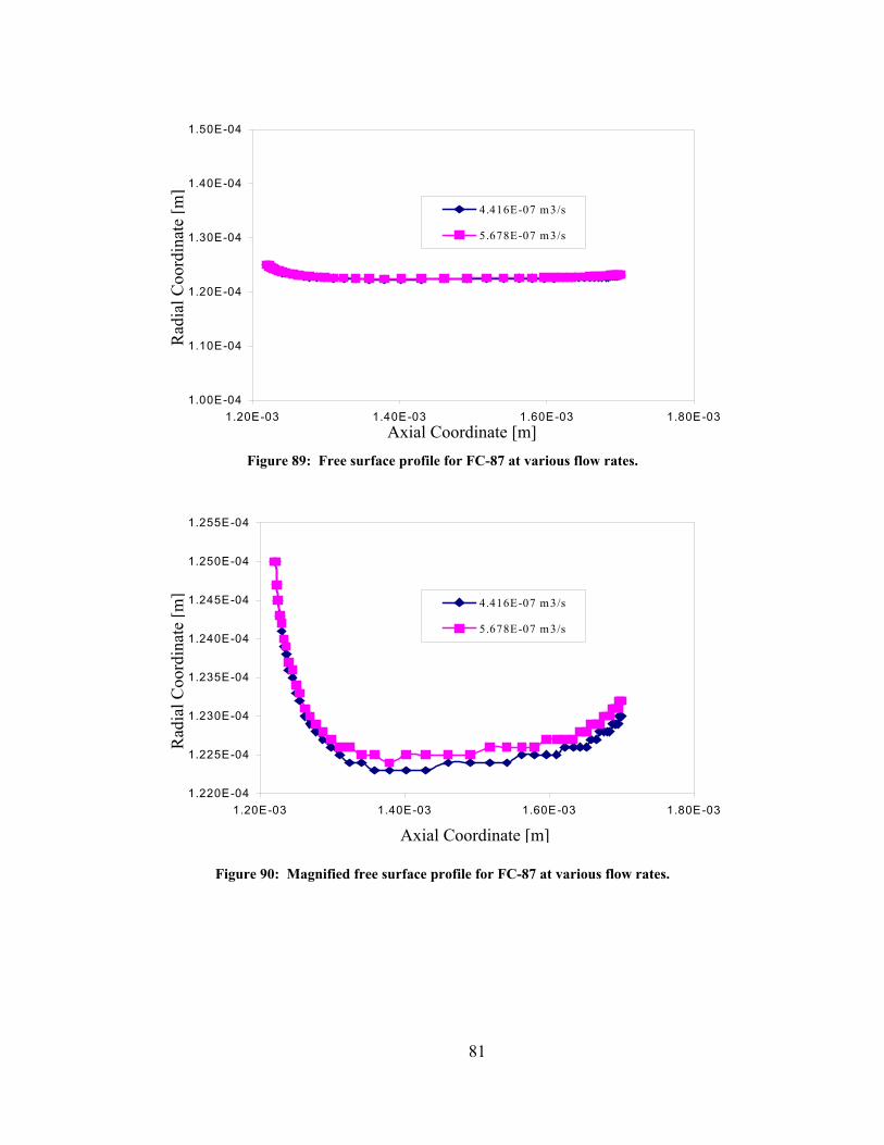
81
1.00E-04
1.10E-04
1.20E-04
1.30E-04
1.40E-04
1.50E-04
1.20E-03 1.40E-03 1.60E-03 1.80E-03
4.416E-07 m3/s
5.678E-07 m3/s
Figure 89: Free surface profile for FC-87 at various flow rates.
1.220E-04
1.225E-04
1.230E-04
1.235E-04
1.240E-04
1.245E-04
1.250E-04
1.255E-04
1.20E-03 1.40E-03 1.60E-03 1.80E-03
4.416E-07 m3/s
5.678E-07 m3/s
Figure 90: Magnified free surface profile for FC-87 at various flow rates.
Axial Coordinate [m]
Rad
ial C
oord
inat
e [m
]
Axial Coordinate [m]
Rad
ial C
oord
inat
e [m
]

82
5.2.4 Methanol
Figure 91 shows the velocity vector plot for Methanol as the working fluid
flowing at 4.416 x 10⁻⁷ m3/s. The maximum velocity was found to be around 8.78
m/s, located near the outlet section of the nozzle. The free surface began at an initial
height of 1.250 x 10⁻⁴ m, but decreased to a final height of 1.220 x 10⁻⁴ m.
Figure 91: Velocity vector plot for Methanol (Q = 4.416 x 10⁻⁷ m3/s). Units are cm/s.
Figures 92 and 93 show the pressure and streamline contour plots,
respectively. The maximum pressure within the nozzle was found to be 3.41 x 10⁴
Pa, while the minimum pressure was -8.71 x 10³ Pa. The inlet-to-outlet pressure
drop was calculated to be about 3.41 x 10⁴ Pa. The streamline contour plot also
shows the fluid entering closed to the center of nozzle flows slightly outward in the
radial direction as it moved toward the outlet.
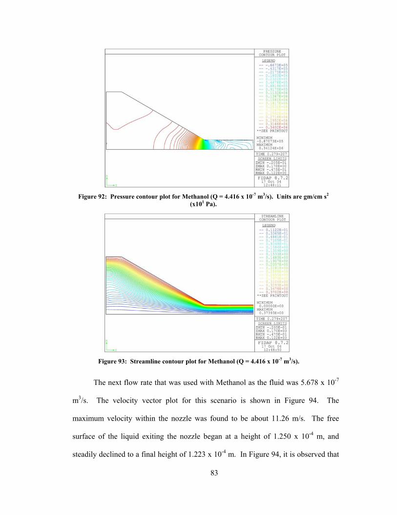
83
Figure 92: Pressure contour plot for Methanol (Q = 4.416 x 10⁻⁷ m3/s). Units are gm/cm s2
(x101 Pa).
Figure 93: Streamline contour plot for Methanol (Q = 4.416 x 10⁻⁷ m3/s).
The next flow rate that was used with Methanol as the fluid was 5.678 x 10⁻⁷
m3/s. The velocity vector plot for this scenario is shown in Figure 94. The
maximum velocity within the nozzle was found to be about 11.26 m/s. The free
surface of the liquid exiting the nozzle began at a height of 1.250 x 10⁻⁴ m, and
steadily declined to a final height of 1.223 x 10⁻⁴ m. In Figure 94, it is observed that
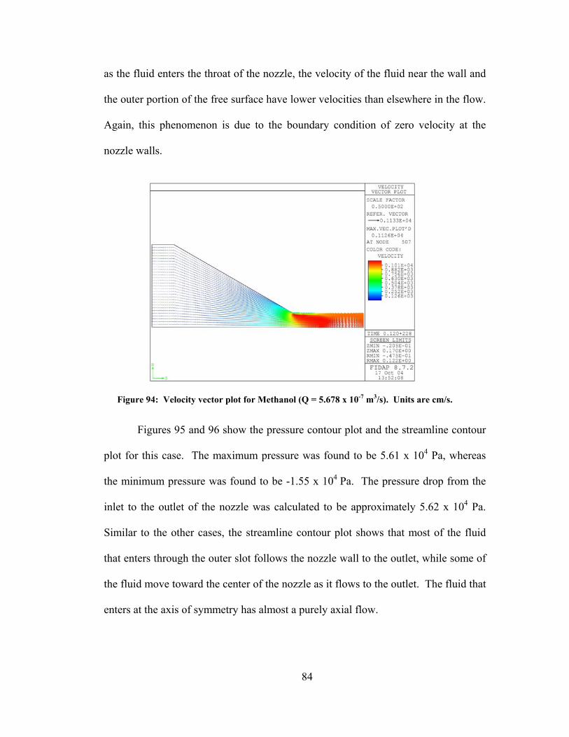
84
as the fluid enters the throat of the nozzle, the velocity of the fluid near the wall and
the outer portion of the free surface have lower velocities than elsewhere in the flow.
Again, this phenomenon is due to the boundary condition of zero velocity at the
nozzle walls.
Figure 94: Velocity vector plot for Methanol (Q = 5.678 x 10⁻⁷ m3/s). Units are cm/s.
Figures 95 and 96 show the pressure contour plot and the streamline contour
plot for this case. The maximum pressure was found to be 5.61 x 10⁴ Pa, whereas
the minimum pressure was found to be -1.55 x 10⁴ Pa. The pressure drop from the
inlet to the outlet of the nozzle was calculated to be approximately 5.62 x 10⁴ Pa.
Similar to the other cases, the streamline contour plot shows that most of the fluid
that enters through the outer slot follows the nozzle wall to the outlet, while some of
the fluid move toward the center of the nozzle as it flows to the outlet. The fluid that
enters at the axis of symmetry has almost a purely axial flow.

85
Figure 95: Pressure contour plot for Methanol (Q = 5.678 x 10⁻⁷ m3/s). Units are gm/cm s2
(x101 Pa).
Figure 96: Streamline contour plot for Methanol (Q = 5.678 x 10⁻⁷ m3/s).
Figures 97 and 98 depict the profile of the free surface obtained when the
working fluid was Methanol. It was noted that the inlet flow rate had little effect on
the height of the free surface; however, 5.678 x 10⁻⁷ m3/s produced a slightly greater
height.

86
1.00E -04
1.10E -04
1.20E -04
1.30E -04
1.40E -04
1.50E -04
1.20E-03 1.40E -03 1.60E-03 1.80E -03
4 .416E -07 m 3/s
5 .678E -07 m 3/s
Figure 97: Free surface profile for Methanol at various flow rates.
1.210E -04
1.215E -04
1.220E -04
1.225E -04
1.230E -04
1.235E -04
1.240E -04
1.245E -04
1.250E -04
1.255E -04
1.20E -03 1.40E -03 1.60E -03 1.80E -03
4 .416E -07 m 3/s
5 .678E -07 m 3/s
Figure 98: Magnified free surface profile for Methanol at various flow rates.
Axial Coordinate [m]
Rad
ial C
oord
inat
e [m
]
Axial Coordinate [m]
Rad
ial C
oord
inat
e [m
]
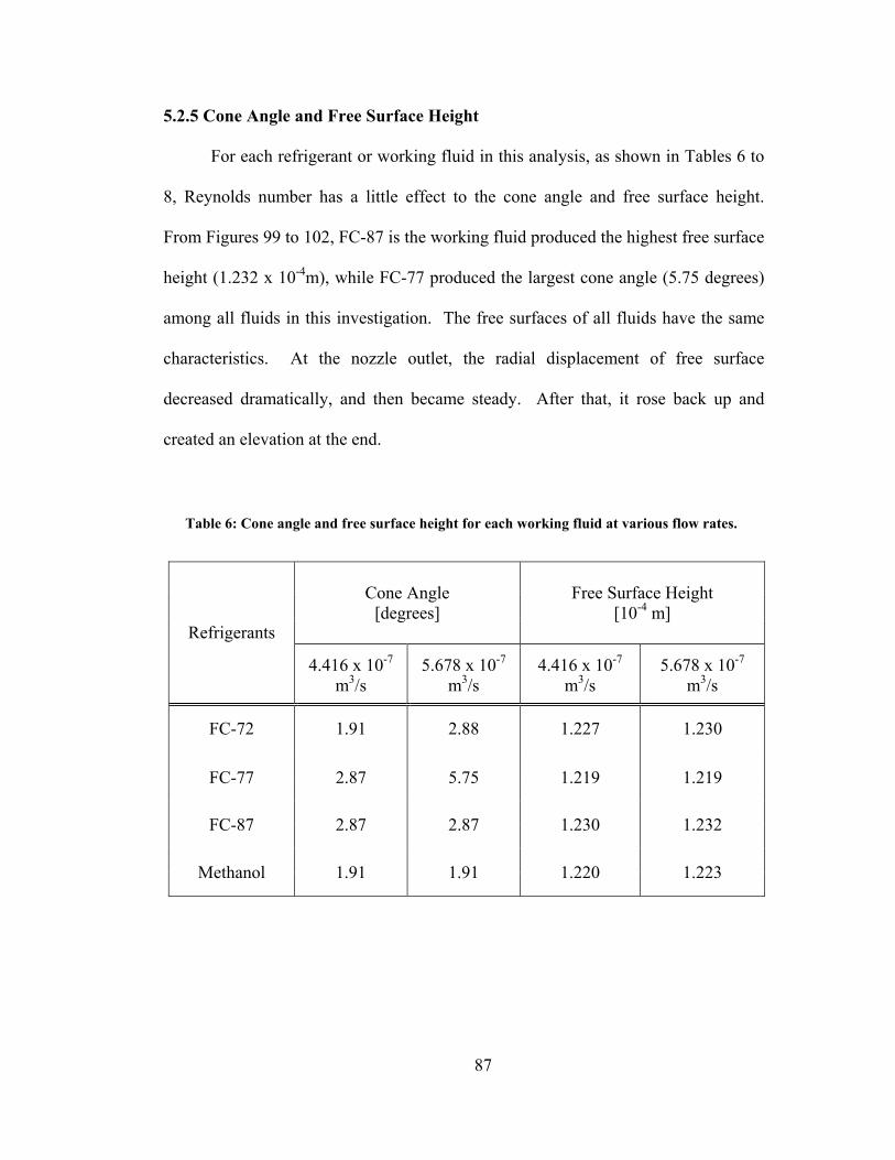
87
5.2.5 Cone Angle and Free Surface Height
For each refrigerant or working fluid in this analysis, as shown in Tables 6 to
8, Reynolds number has a little effect to the cone angle and free surface height.
From Figures 99 to 102, FC-87 is the working fluid produced the highest free surface
height (1.232 x 10⁻⁴m), while FC-77 produced the largest cone angle (5.75 degrees)
among all fluids in this investigation. The free surfaces of all fluids have the same
characteristics. At the nozzle outlet, the radial displacement of free surface
decreased dramatically, and then became steady. After that, it rose back up and
created an elevation at the end.
Cone Angle [degrees]
Free Surface Height [10-4 m]
Refrigerants
4.416 x 10⁻⁷
m3/s 5.678 x 10⁻⁷
m3/s 4.416 x 10⁻⁷
m3/s 5.678 x 10⁻⁷
m3/s
FC-72 1.91 2.88 1.227 1.230
FC-77 2.87 5.75 1.219 1.219
FC-87 2.87 2.87 1.230 1.232
Methanol 1.91 1.91 1.220 1.223
Table 6: Cone angle and free surface height for each working fluid at various flow rates.
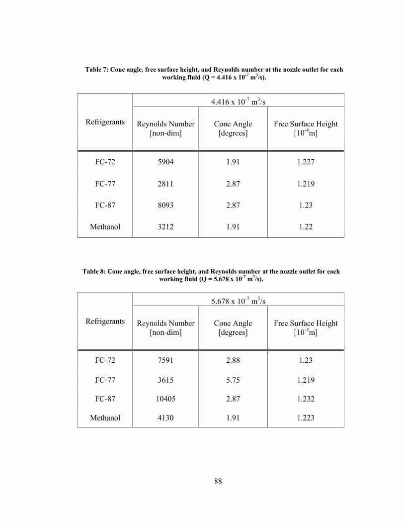
88
4.416 x 10⁻⁷ m3/s
Refrigerants Reynolds Number [non-dim]
Cone Angle [degrees]
Free Surface Height [10-4m]
FC-72 5904 1.91 1.227
FC-77 2811 2.87 1.219
FC-87 8093 2.87 1.23
Methanol 3212 1.91 1.22
5.678 x 10⁻⁷ m3/s
Refrigerants Reynolds Number [non-dim]
Cone Angle [degrees]
Free Surface Height [10-4m]
FC-72 7591 2.88 1.23
FC-77 3615 5.75 1.219
FC-87 10405 2.87 1.232
Methanol 4130 1.91 1.223
Table 7: Cone angle, free surface height, and Reynolds number at the nozzle outlet for each working fluid (Q = 4.416 x 10⁻⁷ m3/s).
Table 8: Cone angle, free surface height, and Reynolds number at the nozzle outlet for eachworking fluid (Q = 5.678 x 10⁻⁷ m3/s).
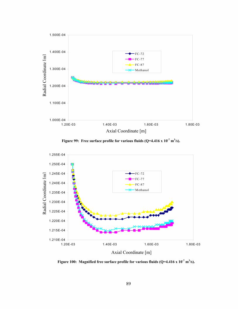
89
1.000E-04
1.100E-04
1.200E-04
1.300E-04
1.400E-04
1.500E-04
1.20E-03 1.40E-03 1.60E-03 1.80E-03
FC-72
FC-77
FC-87
M ethanol
1.210E-04
1.215E-04
1.220E-04
1.225E-04
1.230E-04
1.235E-04
1.240E-04
1.245E-04
1.250E-04
1.255E-04
1.20E-03 1.40E-03 1.60E-03 1.80E-03
FC-72
FC-77
FC-87
M ethanol
Axial Coordinate [m]
Rad
ial C
oord
inat
e [m
]
Figure 100: Magnified free surface profile for various fluids (Q=4.416 x 10⁻⁷ m3/s).
Figure 99: Free surface profile for various fluids (Q=4.416 x 10⁻⁷ m3/s).
Axial Coordinate [m]
Rad
ial C
oord
inat
e [m
]

90
1.000E-04
1.100E-04
1.200E-04
1.300E-04
1.400E-04
1.500E-04
1.20E-03 1.40E-03 1.60E-03 1.80E-03
FC-72FC-77FC-87M ethanol
1.215E-04
1.220E-04
1.225E-04
1.230E-04
1.235E-04
1.240E-04
1.245E-04
1.250E-04
1.255E-04
1.20E-03 1.40E-03 1.60E-03 1.80E-03
FC-72FC-77FC-87M ethanol
Figure 101: Free surface profile for various fluids (Q=5.678 x 10⁻⁷ m3/s).
Axial Coordinate [m]
Rad
ial C
oord
inat
e [m
]
Figure 102: Magnified free surface profile for various fluids (Q=5.678 x 10⁻⁷ m3/s).
Axial Coordinate [m]
Rad
ial C
oord
inat
e [m
]
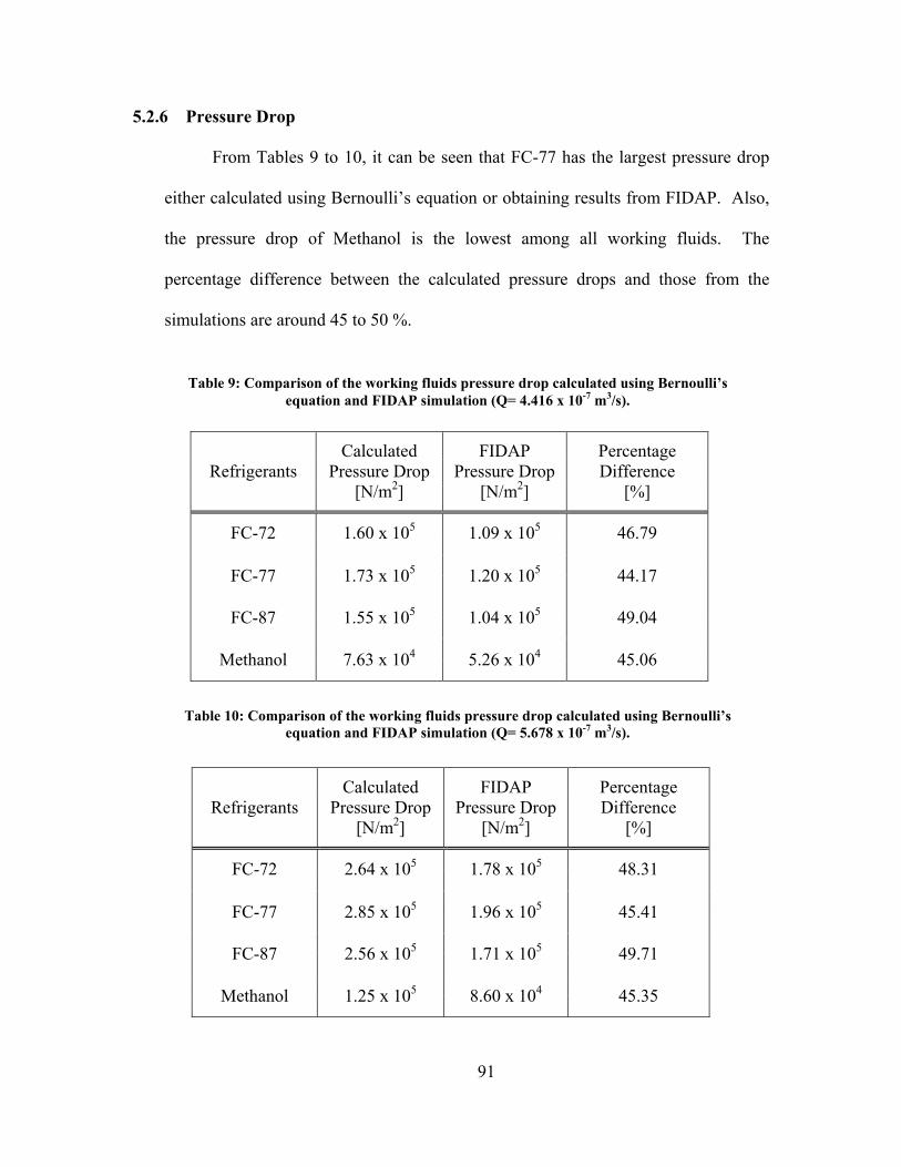
91
5.2.6 Pressure Drop
From Tables 9 to 10, it can be seen that FC-77 has the largest pressure drop
either calculated using Bernoulli’s equation or obtaining results from FIDAP. Also,
the pressure drop of Methanol is the lowest among all working fluids. The
percentage difference between the calculated pressure drops and those from the
simulations are around 45 to 50 %.
Refrigerants Calculated
Pressure Drop [N/m2]
FIDAP Pressure Drop
[N/m2]
Percentage Difference
[%]
FC-72 1.60 x 10⁵ 1.09 x 10⁵ 46.79
FC-77 1.73 x 10⁵ 1.20 x 10⁵ 44.17
FC-87 1.55 x 10⁵ 1.04 x 10⁵ 49.04
Methanol 7.63 x 10⁴ 5.26 x 10⁴ 45.06
Refrigerants Calculated
Pressure Drop [N/m2]
FIDAP Pressure Drop
[N/m2]
Percentage Difference
[%]
FC-72 2.64 x 10⁵ 1.78 x 10⁵ 48.31
FC-77 2.85 x 10⁵ 1.96 x 10⁵ 45.41
FC-87 2.56 x 10⁵ 1.71 x 10⁵ 49.71
Methanol 1.25 x 10⁵ 8.60 x 10⁴ 45.35
Table 9: Comparison of the working fluids pressure drop calculated using Bernoulli’s equation and FIDAP simulation (Q= 4.416 x 10⁻⁷ m3/s).
Table 10: Comparison of the working fluids pressure drop calculated using Bernoulli’s equation and FIDAP simulation (Q= 5.678 x 10⁻⁷ m3/s).

92
5.2.7 Cavitation
Cavitation happens when the liquid pressure falls below the saturation
pressure for that particular fluid. The fluid evaporates at the boundary surface, and
the tiny bubbles becomes a thin gas layer. It may eventually erode and destroy the
system, or prevent the heat conduction process across the boundary surface. Table
11 is the quantitative explanation to show whether the refrigerant creates cavitation
at flow rate either 4.416 x 10⁻⁷ or 5.678 x 10⁻⁷ m3/s in the nozzle. FC-72 and
methanol produced cavitation when the flow rate was 4.416 x 10⁻⁷ m3/s. Next, there
was a cavitation for FC-87 in both flow rates. On the other hand, FC-77 never
produced cavitation in both flow rate trials.
Saturation Pressure
Reynolds Number
Minimum Pressure
Pressure Difference
Cavitation Number
Psat Re Pmin Pmin - Psat Ca Refrigerants
[Pa] [non-dim] [Pa] [Pa] [non-dim] 5904 21800 -9100 -0.1339 FC-72 30900 7591 37700 6800 0.0606 2811 18800 13180 0.1830
FC-77 5620 3615 34400 28780 0.2420 8093 22300 -58800 -0.8915
FC-87 81100 10405 38000 -43100 -0.3957 3212 8710 -1290 -0.0406
Methanol 10000 4130 15500 5500 0.1048
Table 11: Cavitation number of various refrigerants at different Reynolds numbers.
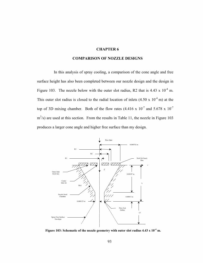
93
CHAPTER 6
COMPARISON OF NOZZLE DESIGNS
In this analysis of spray cooling, a comparison of the cone angle and free
surface height has also been completed between our nozzle design and the design in
Figure 103. The nozzle below with the outer slot radius, R2 that is 4.43 x 10⁻⁴ m.
This outer slot radius is closed to the radial location of inlets (4.50 x 10⁻⁴ m) at the
top of 3D mixing chamber. Both of the flow rates (4.416 x 10⁻⁷ and 5.678 x 10⁻⁷
m3/s) are used at this section. From the results in Table 11, the nozzle in Figure 103
produces a larger cone angle and higher free surface than my design.
R1 R2
R3 0.000743 m
0.00107 m
0.00015 m
L
0.000125 m
R(r)
Nozzle Swirl Chamber
Center Inlet Jet
Outer Inlet Swirl Jets
Swirl Jet Insert Disc
Flow Inlet
Flow Exit Orifice
Spray Free Surface Envelope
Lf
Z
r
Figure 103: Schematic of the nozzle geometry with outer slot radius 4.43 x 10⁻⁴ m.
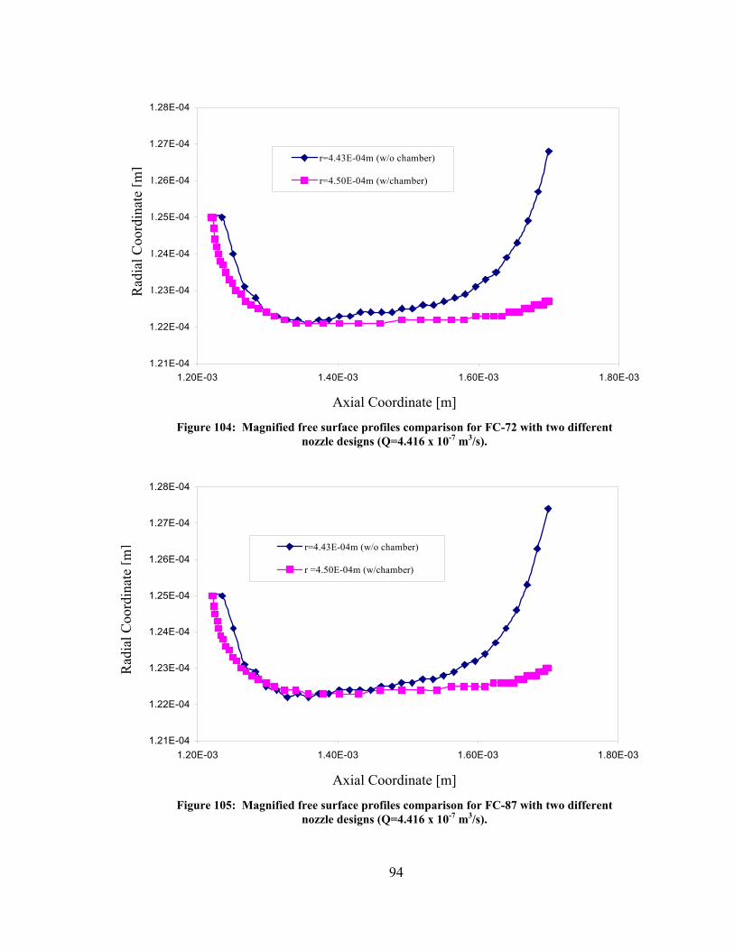
94
1.21E-04
1.22E-04
1.23E-04
1.24E-04
1.25E-04
1.26E-04
1.27E-04
1.28E-04
1.20E-03 1.40E-03 1.60E-03 1.80E-03
r=4.43E-04m (w/o chamber)
r=4.50E-04m (w/chamber)
1.21E-04
1.22E-04
1.23E-04
1.24E-04
1.25E-04
1.26E-04
1.27E-04
1.28E-04
1.20E-03 1.40E-03 1.60E-03 1.80E-03
r=4.43E-04m (w/o chamber)
r =4.50E-04m (w/chamber)
Axial Coordinate [m]
Figure 104: Magnified free surface profiles comparison for FC-72 with two different nozzle designs (Q=4.416 x 10⁻⁷ m3/s).
Rad
ial C
oord
inat
e [m
]
Figure 105: Magnified free surface profiles comparison for FC-87 with two different nozzle designs (Q=4.416 x 10⁻⁷ m3/s).
Axial Coordinate [m]
Rad
ial C
oord
inat
e [m
]
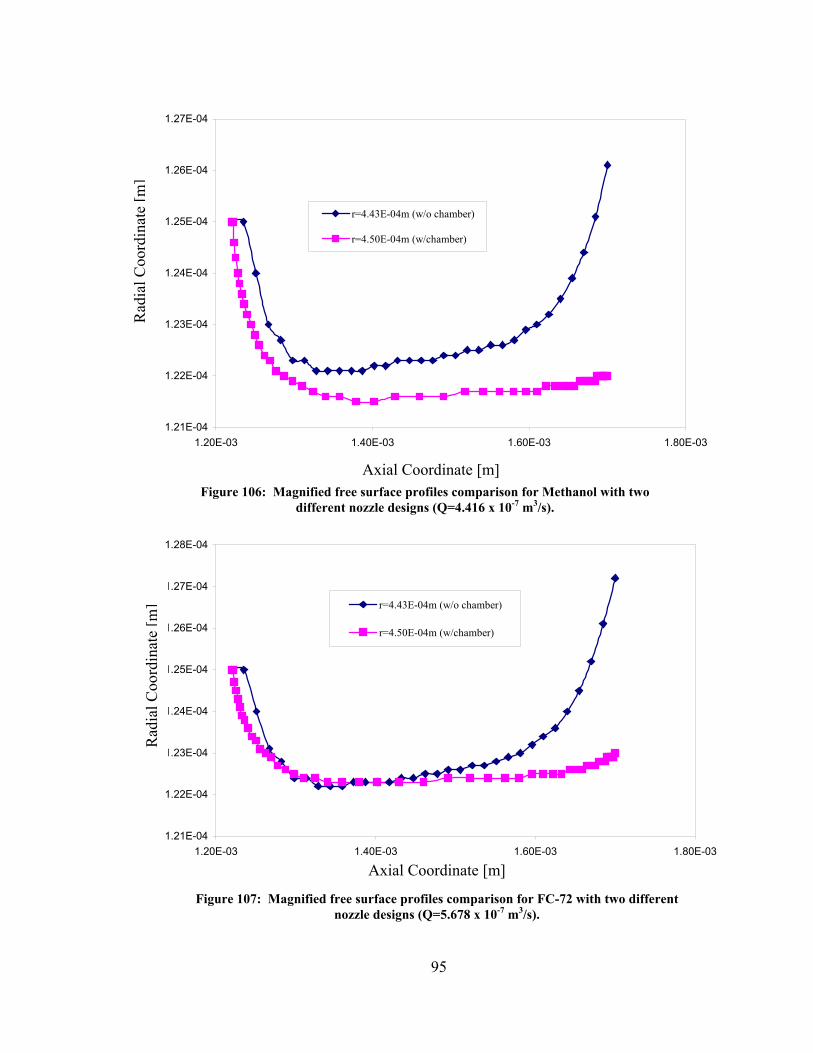
95
1.21E-04
1.22E-04
1.23E-04
1.24E-04
1.25E-04
1.26E-04
1.27E-04
1.20E-03 1.40E-03 1.60E-03 1.80E-03
r=4.43E-04m (w/o chamber)
r=4.50E-04m (w/chamber)
1.21E-04
1.22E-04
1.23E-04
1.24E-04
1.25E-04
1.26E-04
1.27E-04
1.28E-04
1.20E-03 1.40E-03 1.60E-03 1.80E-03
r=4.43E-04m (w/o chamber)
r=4.50E-04m (w/chamber)
Axial Coordinate [m]
Rad
ial C
oord
inat
e [m
]
Figure 106: Magnified free surface profiles comparison for Methanol with two different nozzle designs (Q=4.416 x 10⁻⁷ m3/s).
Axial Coordinate [m]
Figure 107: Magnified free surface profiles comparison for FC-72 with two different nozzle designs (Q=5.678 x 10⁻⁷ m3/s).
Rad
ial C
oord
inat
e [m
]
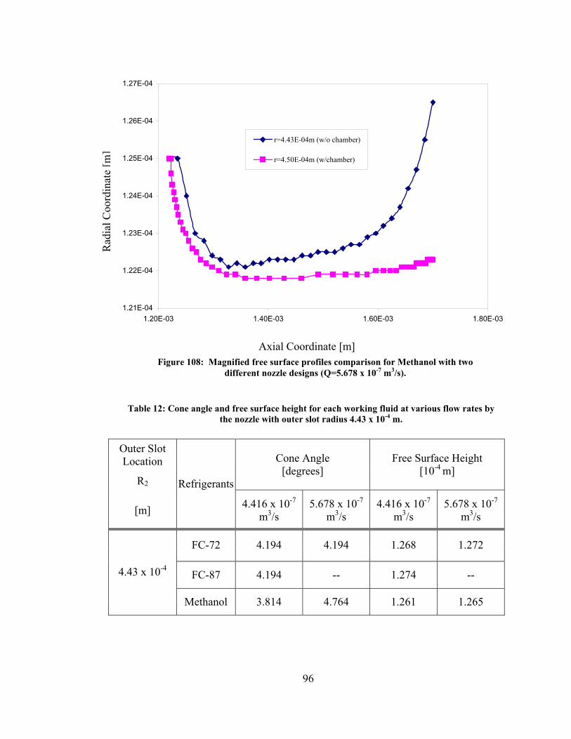
96
1.21E-04
1.22E-04
1.23E-04
1.24E-04
1.25E-04
1.26E-04
1.27E-04
1.20E-03 1.40E-03 1.60E-03 1.80E-03
r=4.43E-04m (w/o chamber)
r=4.50E-04m (w/chamber)
Outer Slot Location
R2
Cone Angle [degrees]
Free Surface Height [10-4 m]
[m]
Refrigerants
4.416 x 10⁻⁷ m3/s
5.678 x 10⁻⁷ m3/s
4.416 x 10⁻⁷ m3/s
5.678 x 10⁻⁷ m3/s
FC-72 4.194 4.194 1.268 1.272
FC-87 4.194 -- 1.274 -- 4.43 x 10⁻⁴
Methanol 3.814 4.764 1.261 1.265
Figure 108: Magnified free surface profiles comparison for Methanol with two different nozzle designs (Q=5.678 x 10⁻⁷ m3/s).
Axial Coordinate [m]
Rad
ial C
oord
inat
e [m
]
Table 12: Cone angle and free surface height for each working fluid at various flow rates by the nozzle with outer slot radius 4.43 x 10⁻⁴ m.
97
CHAPTER 7
CONCLUSIONS AND RECOMMENDATIONS
Based on the 3D and 2D simulations, the conclusion can be drawn as the following:
1. During the increase of volumetric flow rate, the velocities in radial,
circumferential, and axial directions inside the entire system are increased.
2. The fluid pressure decreases gradually from the inlets to the nozzle outlet.
3. The fluid flowing profiles get stabilized as the fluid approaches to the bottom of
chamber.
4. Disorder, efficient mixing, and vorticity can be obviously seen in the chamber
and nozzle, as the flow is turbulent.
5. According to the velocity plot inside the chamber, clockwise spinning and eddy
circulation of fluid can be found in the mixing chamber.
6. Cone angle and free surface height increase when the volumetric flow rates of
FC-72, FC-77, FC-87, and Methanol increase.
7. Among all working fluid in this analysis, FC-87 produces the highest free
surface height in both flow rates, while FC-77 has the lowest.
8. Calculated pressure drop is reasonably higher than the pressure drop found by
computer simulation because Bernoulli’s equation, which is for ideal flow,
ignores the effect created by shear and viscosity of the fluid.
98
9. In the comparison with our nozzle design, the nozzle without mixing chamber
produces larger cone angle and free surface height.
10. The results may be improved by increasing the amount of element in the mesh.
11. The mesh quality should be examined and improved.
12. More data may be obtained at the outlet of mixing chamber for the computation
of averaged radial, circumferential, and axial velocities.
13. More volumetric flow rate may be applied to the simulation.
99
REFERENCES
Burmeister, L.C., Convective Heat Transfer, Wiley, New York, 1993. Ciofalo, M., DiPiazza, I., Brucato, V., “Investigation of Cooling of Hot Walls by
Liquid Water Sprays,” International Journal of Heat and Mass Transfer, Vol. 42, No. 7, 1999, pp. 1157-1175.
Datta, A., and Som, S.K., “Numerical Prediction of Air Core Diameter Coefficient of
Discharge and Spray Cone Angle of a Swirl Spray Pressure Nozzle,” International Journal of Heat and Fluid Flow, Vol. 21, No. 4, 2000, pp. 412-419.
Dumouchel, C., Blook, M. I. G., Dimbrowski, N., Ingham, D. B., and Ledoux, M.,
“Viscous Flow in a Swirl Atomizer,” Chemical Engineering Science, Vol. 48, No. 1, 1993, pp. 81-87.
Gavaises, M., Arcoumanis, C., “Modeling of Sprays from High-Pressure Swirl
Atomizers,” International Journal of Engine Research, Vol. 2, No. 2, 2001, pp. 95-117.
Guarino, J.R., Manno, V.P., “Characterization of Laminar Jet Impingement Cooling
in Portable Computer Applications,” IEEE Transactions on Components and Packaging Technologies, Vol. 25, No. 3, September 2002.
Fabbri, M., Jiang, S., and Dhir, V.K., “Experimental Investigation of Single Phase
Micro Jets Impingement Cooling for Electronic Applications,” 2003 ASME Summer Conference Paper, pp. 1,4, and 7.
Jeng, S. M., Jog, M. A., and Benjamin, M. A., “Computation and Experimental
Study of Liquid Sheet Emanating from Simplex Fuel Nozzle,” AIAA Journal, Vol. 36, No. 2, 1998, pp. 201-207.
Miller, P.C.H., and Ellis, M.C., “Effects of Formulation of Spray Nozzle
Performance for Applications from Ground-Based Boom Sprayers,” Crop Protection, Vol. 19, No. 8-10, 2000, pp. 609-615.
Rothe, P.H., and Block, J.A., “Aerodynamic Behavior of Liquid Sprays,”
International Journal of Multiphase Flow, Vol. 3, No. 3, 1977, pp. 263-272.
100
Sakman, A. T., Jog, M. A., Jeng, S. M., and Benjamin, M. A., “Parametric Study of Simplex Fuel Nozzle Internal Flow and Performance,” AIAA Journal, Vol. 38, No. 7, 2000, pp. 1214-1218.
Som, S.K., and Biswas, G., “Dispersion of Spray from Swirl Nozzles,” Chemical
Engineering and Processing, Vol. 20, No. 4, 1986, pp. 191-200. Wang, E.N., Zhang, L., Jiang, L., Koo, J.M., Goodson, K.E., and Kenny, T.W.,”
Micromachined Jet Arrays for Liquid Impingement Cooling of VLSI Chips,” Mechanical Engineering, Stanford University, 2002.
White, Frank M. Fluid Mechanics: Fourth Edition, Boston, McGraw-Hill, 1999.
Wu, S., Mai, J., Tai, Y.C., and Ho, C.M.,”Micro Heat Exchanger by Using MEMS
Impinging Jets,” Electrical Engineering, California Institute of Technology, 1999.
101
APPENDICES
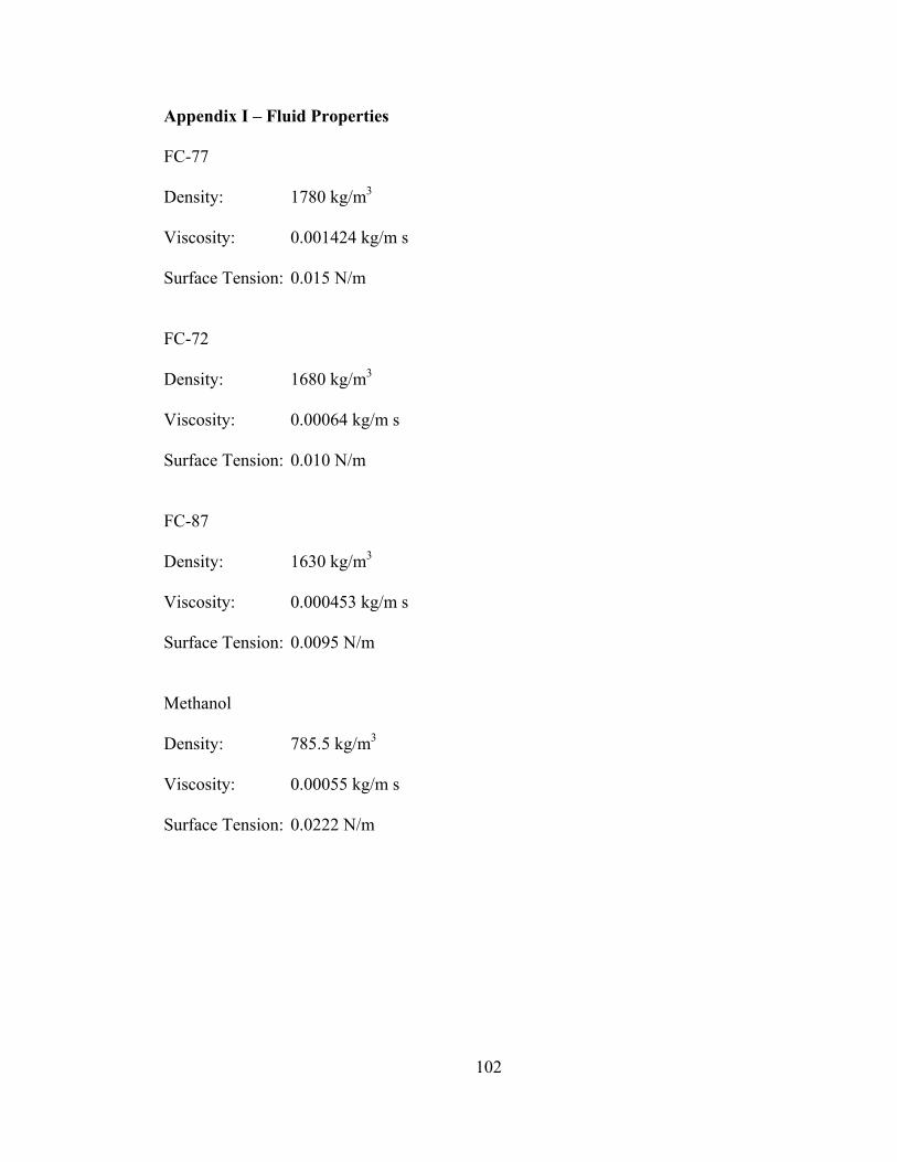
102
Appendix I – Fluid Properties
FC-77 Density: 1780 kg/m3 Viscosity: 0.001424 kg/m s Surface Tension: 0.015 N/m FC-72 Density: 1680 kg/m3 Viscosity: 0.00064 kg/m s Surface Tension: 0.010 N/m FC-87 Density: 1630 kg/m3 Viscosity: 0.000453 kg/m s Surface Tension: 0.0095 N/m Methanol Density: 785.5 kg/m3 Viscosity: 0.00055 kg/m s Surface Tension: 0.0222 N/m
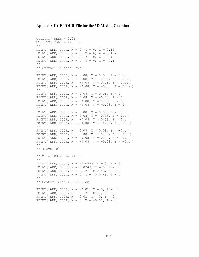
103
Appendix II: FIJOUR File for the 3D Mixing Chamber
UTILITY( SELE = 0.01 ) UTILITY( TOLE = 1e-06 ) // POINT( ADD, COOR, X = 0, Y = 0, Z = 0.15 ) POINT( ADD, COOR, X = 0, Y = 0, Z = 0.1 ) POINT( ADD, COOR, X = 0, Y = 0, Z = 0 ) POINT( ADD, COOR, X = 0, Y = 0, Z = -0.1 ) // // Surface on each Level // POINT( ADD, COOR, X = 0.08, Y = 0.08, Z = 0.15 ) POINT( ADD, COOR, X = 0.08, Y = -0.08, Z = 0.15 ) POINT( ADD, COOR, X = -0.08, Y = 0.08, Z = 0.15 ) POINT( ADD, COOR, X = -0.08, Y = -0.08, Z = 0.15 ) // POINT( ADD, COOR, X = 0.08, Y = 0.08, Z = 0 ) POINT( ADD, COOR, X = 0.08, Y = -0.08, Z = 0 ) POINT( ADD, COOR, X = -0.08, Y = 0.08, Z = 0 ) POINT( ADD, COOR, X = -0.08, Y = -0.08, Z = 0 ) // POINT( ADD, COOR, X = 0.08, Y = 0.08, Z = 0.1 ) POINT( ADD, COOR, X = 0.08, Y = -0.08, Z = 0.1 ) POINT( ADD, COOR, X = -0.08, Y = 0.08, Z = 0.1 ) POINT( ADD, COOR, X = -0.08, Y = -0.08, Z = 0.1 ) // POINT( ADD, COOR, X = 0.08, Y = 0.08, Z = -0.1 ) POINT( ADD, COOR, X = 0.08, Y = -0.08, Z = -0.1 ) POINT( ADD, COOR, X = -0.08, Y = 0.08, Z = -0.1 ) POINT( ADD, COOR, X = -0.08, Y = -0.08, Z = -0.1 ) // // (Level 0) // // Outer Edge (Level 0) // POINT( ADD, COOR, X = -0.0743, Y = 0, Z = 0 ) POINT( ADD, COOR, X = 0.0743, Y = 0, Z = 0 ) POINT( ADD, COOR, X = 0, Y = 0.0743, Z = 0 ) POINT( ADD, COOR, X = 0, Y = -0.0743, Z = 0 ) // // Center Inlet r = 0.01 cm // POINT( ADD, COOR, X = -0.01, Y = 0, Z = 0 ) POINT( ADD, COOR, X = 0, Y = 0.01, Z = 0 ) POINT( ADD, COOR, X = 0.01, Y = 0, Z = 0 ) POINT( ADD, COOR, X = 0, Y = -0.01, Z = 0 )
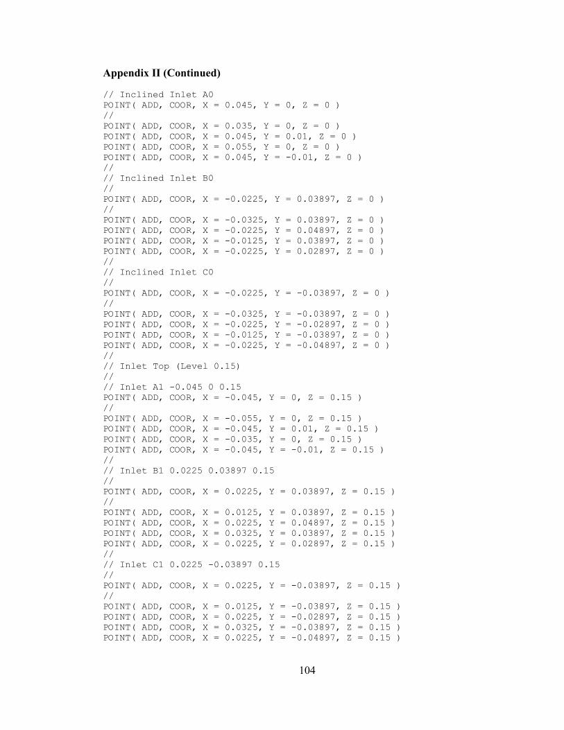
104
Appendix II (Continued)
// Inclined Inlet A0 POINT( ADD, COOR, X = 0.045, Y = 0, Z = 0 ) // POINT( ADD, COOR, X = 0.035, Y = 0, Z = 0 ) POINT( ADD, COOR, X = 0.045, Y = 0.01, Z = 0 ) POINT( ADD, COOR, X = 0.055, Y = 0, Z = 0 ) POINT( ADD, COOR, X = 0.045, Y = -0.01, Z = 0 ) // // Inclined Inlet B0 // POINT( ADD, COOR, X = -0.0225, Y = 0.03897, Z = 0 ) // POINT( ADD, COOR, X = -0.0325, Y = 0.03897, Z = 0 ) POINT( ADD, COOR, X = -0.0225, Y = 0.04897, Z = 0 ) POINT( ADD, COOR, X = -0.0125, Y = 0.03897, Z = 0 ) POINT( ADD, COOR, X = -0.0225, Y = 0.02897, Z = 0 ) // // Inclined Inlet C0 // POINT( ADD, COOR, X = -0.0225, Y = -0.03897, Z = 0 ) // POINT( ADD, COOR, X = -0.0325, Y = -0.03897, Z = 0 ) POINT( ADD, COOR, X = -0.0225, Y = -0.02897, Z = 0 ) POINT( ADD, COOR, X = -0.0125, Y = -0.03897, Z = 0 ) POINT( ADD, COOR, X = -0.0225, Y = -0.04897, Z = 0 ) // // Inlet Top (Level 0.15) // // Inlet A1 -0.045 0 0.15 POINT( ADD, COOR, X = -0.045, Y = 0, Z = 0.15 ) // POINT( ADD, COOR, X = -0.055, Y = 0, Z = 0.15 ) POINT( ADD, COOR, X = -0.045, Y = 0.01, Z = 0.15 ) POINT( ADD, COOR, X = -0.035, Y = 0, Z = 0.15 ) POINT( ADD, COOR, X = -0.045, Y = -0.01, Z = 0.15 ) // // Inlet B1 0.0225 0.03897 0.15 // POINT( ADD, COOR, X = 0.0225, Y = 0.03897, Z = 0.15 ) // POINT( ADD, COOR, X = 0.0125, Y = 0.03897, Z = 0.15 ) POINT( ADD, COOR, X = 0.0225, Y = 0.04897, Z = 0.15 ) POINT( ADD, COOR, X = 0.0325, Y = 0.03897, Z = 0.15 ) POINT( ADD, COOR, X = 0.0225, Y = 0.02897, Z = 0.15 ) // // Inlet C1 0.0225 -0.03897 0.15 // POINT( ADD, COOR, X = 0.0225, Y = -0.03897, Z = 0.15 ) // POINT( ADD, COOR, X = 0.0125, Y = -0.03897, Z = 0.15 ) POINT( ADD, COOR, X = 0.0225, Y = -0.02897, Z = 0.15 ) POINT( ADD, COOR, X = 0.0325, Y = -0.03897, Z = 0.15 ) POINT( ADD, COOR, X = 0.0225, Y = -0.04897, Z = 0.15 )
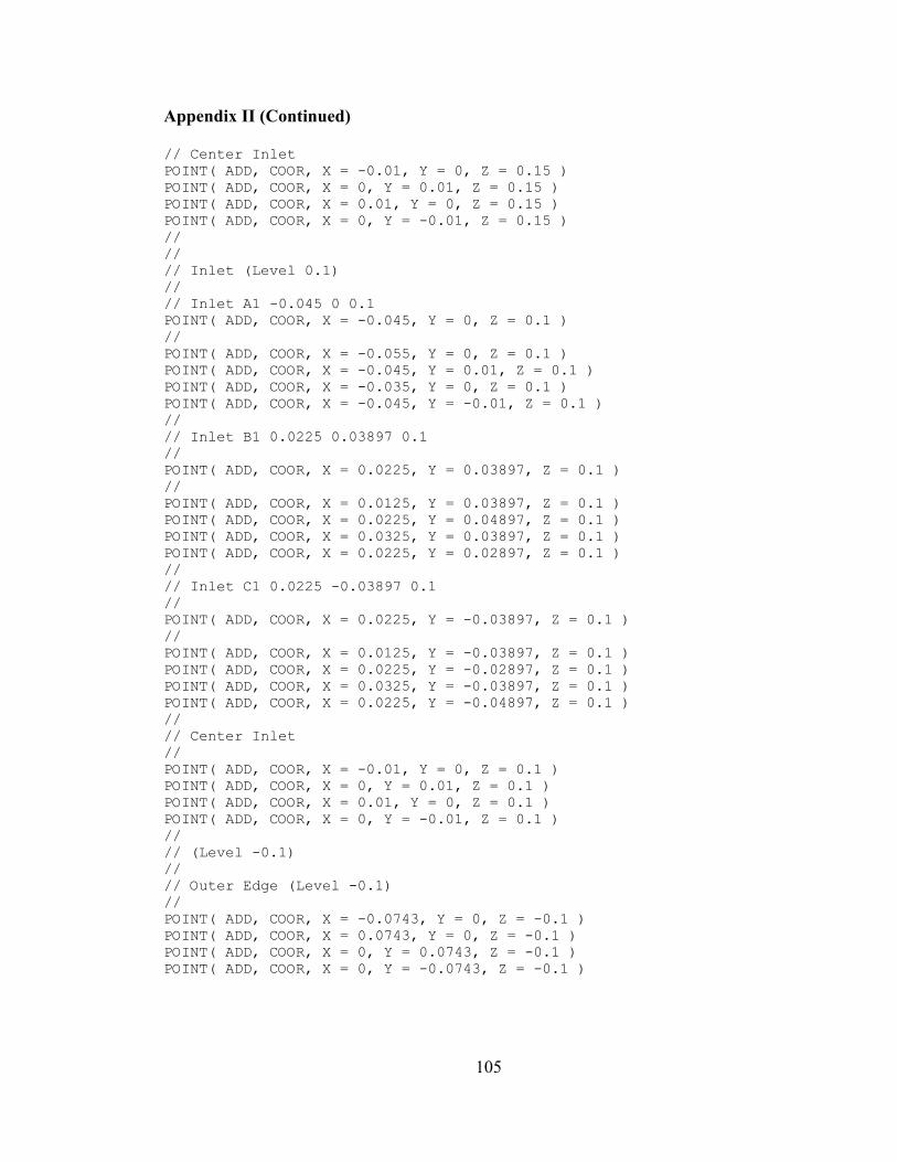
105
Appendix II (Continued) // Center Inlet POINT( ADD, COOR, X = -0.01, Y = 0, Z = 0.15 ) POINT( ADD, COOR, X = 0, Y = 0.01, Z = 0.15 ) POINT( ADD, COOR, X = 0.01, Y = 0, Z = 0.15 ) POINT( ADD, COOR, X = 0, Y = -0.01, Z = 0.15 ) // // // Inlet (Level 0.1) // // Inlet A1 -0.045 0 0.1 POINT( ADD, COOR, X = -0.045, Y = 0, Z = 0.1 ) // POINT( ADD, COOR, X = -0.055, Y = 0, Z = 0.1 ) POINT( ADD, COOR, X = -0.045, Y = 0.01, Z = 0.1 ) POINT( ADD, COOR, X = -0.035, Y = 0, Z = 0.1 ) POINT( ADD, COOR, X = -0.045, Y = -0.01, Z = 0.1 ) // // Inlet B1 0.0225 0.03897 0.1 // POINT( ADD, COOR, X = 0.0225, Y = 0.03897, Z = 0.1 ) // POINT( ADD, COOR, X = 0.0125, Y = 0.03897, Z = 0.1 ) POINT( ADD, COOR, X = 0.0225, Y = 0.04897, Z = 0.1 ) POINT( ADD, COOR, X = 0.0325, Y = 0.03897, Z = 0.1 ) POINT( ADD, COOR, X = 0.0225, Y = 0.02897, Z = 0.1 ) // // Inlet C1 0.0225 -0.03897 0.1 // POINT( ADD, COOR, X = 0.0225, Y = -0.03897, Z = 0.1 ) // POINT( ADD, COOR, X = 0.0125, Y = -0.03897, Z = 0.1 ) POINT( ADD, COOR, X = 0.0225, Y = -0.02897, Z = 0.1 ) POINT( ADD, COOR, X = 0.0325, Y = -0.03897, Z = 0.1 ) POINT( ADD, COOR, X = 0.0225, Y = -0.04897, Z = 0.1 ) // // Center Inlet // POINT( ADD, COOR, X = -0.01, Y = 0, Z = 0.1 ) POINT( ADD, COOR, X = 0, Y = 0.01, Z = 0.1 ) POINT( ADD, COOR, X = 0.01, Y = 0, Z = 0.1 ) POINT( ADD, COOR, X = 0, Y = -0.01, Z = 0.1 ) // // (Level -0.1) // // Outer Edge (Level -0.1) // POINT( ADD, COOR, X = -0.0743, Y = 0, Z = -0.1 ) POINT( ADD, COOR, X = 0.0743, Y = 0, Z = -0.1 ) POINT( ADD, COOR, X = 0, Y = 0.0743, Z = -0.1 ) POINT( ADD, COOR, X = 0, Y = -0.0743, Z = -0.1 )
106
Appendix II (Continued) // Center Inlet r = 0.01 cm // POINT( ADD, COOR, X = -0.01, Y = 0, Z = -0.1 ) POINT( ADD, COOR, X = 0, Y = 0.01, Z = -0.1 ) POINT( ADD, COOR, X = 0.01, Y = 0, Z = -0.1 ) POINT( ADD, COOR, X = 0, Y = -0.01, Z = -0.1 ) // // Inclined Inlet A2 // POINT( ADD, COOR, X = 0.045, Y = 0, Z = -0.1 ) // POINT( ADD, COOR, X = 0.035, Y = 0, Z = -0.1 ) POINT( ADD, COOR, X = 0.045, Y = 0.01, Z = -0.1 ) POINT( ADD, COOR, X = 0.055, Y = 0, Z = -0.1 ) POINT( ADD, COOR, X = 0.045, Y = -0.01, Z = -0.1 ) // // Inclined Inlet B2 // POINT( ADD, COOR, X = -0.0225, Y = 0.03897, Z = -0.1 ) // POINT( ADD, COOR, X = -0.0325, Y = 0.03897, Z = -0.1 ) POINT( ADD, COOR, X = -0.0225, Y = 0.04897, Z = -0.1 ) POINT( ADD, COOR, X = -0.0125, Y = 0.03897, Z = -0.1 ) POINT( ADD, COOR, X = -0.0225, Y = 0.02897, Z = -0.1 ) // // Inclined Inlet C2 // POINT( ADD, COOR, X = -0.0225, Y = -0.03897, Z = -0.1 ) // POINT( ADD, COOR, X = -0.0325, Y = -0.03897, Z = -0.1 ) POINT( ADD, COOR, X = -0.0225, Y = -0.02897, Z = -0.1 ) POINT( ADD, COOR, X = -0.0125, Y = -0.03897, Z = -0.1 ) POINT( ADD, COOR, X = -0.0225, Y = -0.04897, Z = -0.1 )
107
Appendix III: FIPREP File for the 3D Mixing Chamber (Sample:FC-72) FIPREP( ) // // DENSITY OF FC-72 DENSITY( ADD, SET = "fc-72", CONS = 1.68 ) // VISCOSITY OF FC-72 VISCOSITY( ADD, SET = "fc-72", CONS = 0.0064, MIXL ) // SURFACE TENSION OF FC-72 SURFACETENSION( ADD, SET = "fc-72", CONS = 10 ) // //GRAVITY BODYFORCE( ADD, CONS, FX = 0, FY = 0, FZ = -981 ) // DATAPRINT( ADD, CONT ) EXECUTION( ADD, NEWJ ) PRESSURE( ADD, MIXE = 1e-08, DISC ) PRINTOUT( ADD, NONE ) PROBLEM( ADD, 3-D, INCO, STEA, TURB, NONL, NEWT, MOME, ISOT, FIXE, SING ) SOLUTION( ADD, SEGR = 2000, KINE = 25, VELC = 0.001, CGS = 2000, CR = 2000, NCGC = 1e-06, SCGC = 1e-06, SCHA = 0 ) RENUMBER( ADD, PROF ) EDDYVISCOSITY( ADD, SPEZ ) OPTIONS( ADD, UPWI ) UPWINDING( ADD, STRE ) RELAXATION( HYBR ) 0.3, 0.3, 0.3, 0.5, 0, 0, 0, 0 // ENTITY( ADD, NAME = "fluid-01", FLUI, PROP = "fc-72" ) ENTITY( ADD, NAME = "fluid-02", FLUI, PROP = "fc-72" ) ENTITY( ADD, NAME = "fluid-03", FLUI, PROP = "fc-72" ) ENTITY( ADD, NAME = "fluid-04", FLUI, PROP = "fc-72" ) // ENTITY( ADD, NAME = "wall-c-01", WALL ) ENTITY( ADD, NAME = "wall-c-02", WALL ) ENTITY( ADD, NAME = "wall-c-03", WALL ) ENTITY( ADD, NAME = "wall-c-04", WALL ) ENTITY( ADD, NAME = "wall-c-05", WALL ) ENTITY( ADD, NAME = "wall-c-06", WALL ) ENTITY( ADD, NAME = "wall-c-07", WALL ) ENTITY( ADD, NAME = "wall-c-08", WALL ) // ENTITY( ADD, NAME = "wall-01-01", WALL ) ENTITY( ADD, NAME = "wall-01-02", WALL ) ENTITY( ADD, NAME = "wall-01-03", WALL ) ENTITY( ADD, NAME = "wall-01-04", WALL ) ENTITY( ADD, NAME = "wall-01-05", WALL ) ENTITY( ADD, NAME = "wall-01-06", WALL ) ENTITY( ADD, NAME = "wall-01-07", WALL ) ENTITY( ADD, NAME = "wall-01-08", WALL ) //
108
Appendix III (Continued) ENTITY( ADD, NAME = "wall-02-01", WALL ) ENTITY( ADD, NAME = "wall-02-02", WALL ) ENTITY( ADD, NAME = "wall-02-03", WALL ) ENTITY( ADD, NAME = "wall-02-04", WALL ) ENTITY( ADD, NAME = "wall-02-05", WALL ) ENTITY( ADD, NAME = "wall-02-06", WALL ) ENTITY( ADD, NAME = "wall-02-07", WALL ) ENTITY( ADD, NAME = "wall-02-08", WALL ) // ENTITY( ADD, NAME = "wall-03-01", WALL ) ENTITY( ADD, NAME = "wall-03-02", WALL ) ENTITY( ADD, NAME = "wall-03-03", WALL ) ENTITY( ADD, NAME = "wall-03-04", WALL ) ENTITY( ADD, NAME = "wall-03-05", WALL ) ENTITY( ADD, NAME = "wall-03-06", WALL ) ENTITY( ADD, NAME = "wall-03-07", WALL ) ENTITY( ADD, NAME = "wall-03-08", WALL ) // ENTITY( ADD, NAME = "inlet-c", PLOT ) ENTITY( ADD, NAME = "inlet-01", PLOT ) ENTITY( ADD, NAME = "inlet-02", PLOT ) ENTITY( ADD, NAME = "inlet-03", PLOT ) // ENTITY( ADD, NAME = "inlet-top-c", PLOT, ATTA = "fluid-02", NATT = "fluid-01" ) ENTITY( ADD, NAME = "inlet-top-01", PLOT, ATTA = "fluid-02", NATT = "fluid-01" ) ENTITY( ADD, NAME = "inlet-top-02", PLOT, ATTA = "fluid-02", NATT = "fluid-01" ) ENTITY( ADD, NAME = "inlet-top-03", PLOT, ATTA = "fluid-02", NATT = "fluid-01" ) // ENTITY( ADD, NAME = "top-c", PLOT, ATTA = "fluid-03", NATT = "fluid-04" ) ENTITY( ADD, NAME = "top-01", PLOT, ATTA = "fluid-03", NATT = "fluid-04" ) ENTITY( ADD, NAME = "top-02", PLOT, ATTA = "fluid-03", NATT = "fluid-04" ) ENTITY( ADD, NAME = "top-03", PLOT, ATTA = "fluid-03", NATT = "fluid-04" ) // ENTITY( ADD, NAME = "outlet-c", PLOT, ATTA = "fluid-03", NATT = "fluid-04" ) ENTITY( ADD, NAME = "outlet-01", PLOT, ATTA = "fluid-03", NATT = "fluid-04" ) ENTITY( ADD, NAME = "outlet-02", PLOT, ATTA = "fluid-03", NATT = "fluid-04" ) ENTITY( ADD, NAME = "outlet-03", PLOT, ATTA = "fluid-03", NATT = "fluid-04" ) ENTITY( ADD, NAME = "chamber-outlet", PLOT, ATTA = "fluid-04", NATT = "fluid-03" ) // ENTITY( ADD, NAME = "chamber-wall", WALL )
109
Appendix III (Continued) ENTITY( ADD, NAME = "chamber-top", PLOT, ATTA = "fluid-04", NATT = "fluid-03" ) ENTITY( ADD, NAME = "sc-01", PLOT, ATTA = "fluid-03", NATT = "fluid-04" ) ENTITY( ADD, NAME = "sc-02", PLOT, ATTA = "fluid-03", NATT = "fluid-04" ) ENTITY( ADD, NAME = "sc-03", PLOT, ATTA = "fluid-03", NATT = "fluid-04" ) ENTITY( ADD, NAME = "sc-04", PLOT, ATTA = "fluid-03", NATT = "fluid-04" ) // ENTITY( ADD, NAME = "s01-01", PLOT, ATTA = "fluid-03", NATT = "fluid-04" ) ENTITY( ADD, NAME = "s01-02", PLOT, ATTA = "fluid-03", NATT = "fluid-04" ) ENTITY( ADD, NAME = "s01-03", PLOT, ATTA = "fluid-03", NATT = "fluid-04" ) ENTITY( ADD, NAME = "s01-04", PLOT, ATTA = "fluid-03", NATT = "fluid-04" ) // ENTITY( ADD, NAME = "s02-01", PLOT, ATTA = "fluid-03", NATT = "fluid-04" ) ENTITY( ADD, NAME = "s02-02", PLOT, ATTA = "fluid-03", NATT = "fluid-04" ) ENTITY( ADD, NAME = "s02-03", PLOT, ATTA = "fluid-03", NATT = "fluid-04" ) ENTITY( ADD, NAME = "s02-04", PLOT, ATTA = "fluid-03", NATT = "fluid-04" ) // ENTITY( ADD, NAME = "s03-01", PLOT, ATTA = "fluid-03", NATT = "fluid-04" ) ENTITY( ADD, NAME = "s03-02", PLOT, ATTA = "fluid-03", NATT = "fluid-04" ) ENTITY( ADD, NAME = "s03-03", PLOT, ATTA = "fluid-03", NATT = "fluid-04" ) ENTITY( ADD, NAME = "s03-04", PLOT, ATTA = "fluid-03", NATT = "fluid-04" ) // //INLET VELOCITY IS –351, WHEN Q = 4.416 X 10⁻⁷ m3/s BCNODE( ADD, UZ, ENTI = "inlet-c", CONS = -351 ) BCNODE( ADD, UZ, ENTI = "inlet-01", CONS = -351 ) BCNODE( ADD, UZ, ENTI = "inlet-02", CONS = -351 ) BCNODE( ADD, UZ, ENTI = "inlet-03", CONS = -351 ) // //**INLET VELOCITY IS –452, WHEN Q = 5.678 X 10⁻⁷ m3/s** // BCNODE( ADD, VELO, ENTI = "wall-c-01", ZERO, X, Y, Z ) BCNODE( ADD, VELO, ENTI = "wall-c-02", ZERO, X, Y, Z ) BCNODE( ADD, VELO, ENTI = "wall-c-03", ZERO, X, Y, Z ) BCNODE( ADD, VELO, ENTI = "wall-c-04", ZERO, X, Y, Z ) BCNODE( ADD, VELO, ENTI = "wall-c-05", ZERO, X, Y, Z ) BCNODE( ADD, VELO, ENTI = "wall-c-06", ZERO, X, Y, Z ) BCNODE( ADD, VELO, ENTI = "wall-c-07", ZERO, X, Y, Z ) BCNODE( ADD, VELO, ENTI = "wall-c-08", ZERO, X, Y, Z )
110
Appendix III (Continued) BCNODE( ADD, VELO, ENTI = "wall-01-01", ZERO, X, Y, Z ) BCNODE( ADD, VELO, ENTI = "wall-01-02", ZERO, X, Y, Z ) BCNODE( ADD, VELO, ENTI = "wall-01-03", ZERO, X, Y, Z )
BCNODE( ADD, VELO, ENTI = "wall-01-04", ZERO, X, Y, Z ) BCNODE( ADD, VELO, ENTI = "wall-01-05", ZERO, X, Y, Z ) BCNODE( ADD, VELO, ENTI = "wall-01-06", ZERO, X, Y, Z ) BCNODE( ADD, VELO, ENTI = "wall-01-07", ZERO, X, Y, Z ) BCNODE( ADD, VELO, ENTI = "wall-01-08", ZERO, X, Y, Z ) // BCNODE( ADD, VELO, ENTI = "wall-02-01", ZERO, X, Y, Z ) BCNODE( ADD, VELO, ENTI = "wall-02-02", ZERO, X, Y, Z ) BCNODE( ADD, VELO, ENTI = "wall-02-03", ZERO, X, Y, Z ) BCNODE( ADD, VELO, ENTI = "wall-02-04", ZERO, X, Y, Z ) BCNODE( ADD, VELO, ENTI = "wall-02-05", ZERO, X, Y, Z ) BCNODE( ADD, VELO, ENTI = "wall-02-06", ZERO, X, Y, Z ) BCNODE( ADD, VELO, ENTI = "wall-02-07", ZERO, X, Y, Z ) BCNODE( ADD, VELO, ENTI = "wall-02-08", ZERO, X, Y, Z ) // BCNODE( ADD, VELO, ENTI = "wall-03-01", ZERO, X, Y, Z ) BCNODE( ADD, VELO, ENTI = "wall-03-02", ZERO, X, Y, Z ) BCNODE( ADD, VELO, ENTI = "wall-03-03", ZERO, X, Y, Z ) BCNODE( ADD, VELO, ENTI = "wall-03-04", ZERO, X, Y, Z ) BCNODE( ADD, VELO, ENTI = "wall-03-05", ZERO, X, Y, Z ) BCNODE( ADD, VELO, ENTI = "wall-03-06", ZERO, X, Y, Z ) BCNODE( ADD, VELO, ENTI = "wall-03-07", ZERO, X, Y, Z ) BCNODE( ADD, VELO, ENTI = "wall-03-08", ZERO, X, Y, Z ) // BCNODE( ADD, VELO, ENTI = "chamber-wall", ZERO, X, Y, Z ) BCNODE( ADD, VELO, ENTI = "chamber-top", ZERO, X, Y, Z ) // END( )
111
Appendix IV: FIJOUR File for the Small Nozzle with Free Surface (4.416 x 10⁻⁷ and 5.678 x 10⁻⁷ m3/s)
FI-GEN( ELEM = 1, POIN = 1, CURV = 1, SURF = 1, NODE = 0, MEDG = 1, MLOO = 1, MFAC = 1, BEDG = 1, SPAV = 1, MSHE = 1, MSOL = 1, COOR = 1, TOLE = 1e-07 ) WINDOW(CHANGE= 1, MATRIX ) 1.000000 0.000000 0.000000 0.000000 0.000000 1.000000 0.000000 0.000000 0.000000 0.000000 1.000000 0.000000 0.000000 0.000000 0.000000 1.000000 -10.00000 10.00000 -7.50000 7.50000 -7.50000 7.50000 WINDOW( CHAN = 1, MATR ) 1, 0, 0, 0 0, 1, 0, 0 0, 0, 1, 0 0, 0, 0, 1 -10, 10, -7.5, 7.5, -7.5, 7.5 UTILITY( SELE = 0.01 ) POINT( ADD, COOR, X = 0, Y = 0, Z = 0 ) POINT( ADD, COOR, X = 0.107, Y = 0, Z = 0 ) POINT( ADD, COOR, X = 0.122, Y = 0, Z = 0 ) POINT( ADD, COOR, X = 0.17, Y = 0, Z = 0 ) POINT( ADD, COOR, X = 0.17, Y = 0.0125, Z = 0 ) POINT( ADD, COOR, X = 0.122, Y = 0.0125, Z = 0 ) POINT( ADD, COOR, X = 0.107, Y = 0.0125, Z = 0 ) POINT( ADD, COOR, X = 0, Y = 0.0743, Z = 0 ) POINT( ADD, COOR, X = -0.02, Y = 0.0743, Z = 0 ) POINT( ADD, COOR, X = -0.02, Y = 0, Z = 0 ) WINDOW( CHAN = 1, MATR ) 1, 0, 0, 0 0, 1, 0, 0 0, 0, 1, 0 0, 0, 0, 1 -0.02475, 0.17475, -0.03766, 0.11196, -0.1995, 0.1995 45, 45, 45, 45 POINT( ADD, COOR, X = 0.17, Y = 0.0743, Z = 0 ) POINT( SELE, LOCA, WIND = 1 ) 0.0239163, 0.253114 / ID = 10 / ID = 10 0.0269058, 0.743398 / ID = 9 / ID = 9 CURVE( ADD, ORDE = 1 ) POINT( SELE, LOCA, WIND = 1 ) 0.0254111, 0.747384 / ID = 9 / ID = 9 0.124066, 0.75137 / ID = 8 / ID = 8 CURVE( ADD, ORDE = 1 ) POINT( SELE, LOCA, WIND = 1 )
112
Appendix IV (Continued) 0.125561, 0.745391 / ID = 8 / ID = 8 0.662182, 0.334828 / ID = 7 / ID = 7 CURVE( ADD, ORDE = 1 ) POINT( SELE, LOCA, WIND = 1 ) 0.659193, 0.332835 / ID = 7 / ID = 7 0.736921, 0.336821 / ID = 6 / ID = 6 CURVE( ADD, ORDE = 1 ) POINT( SELE, LOCA, WIND = 1 ) 0.736921, 0.328849 / ID = 6 / ID = 6 0.982063, 0.334828 / ID = 5 / ID = 5 CURVE( ADD, ORDE = 1 ) POINT( SELE, LOCA, WIND = 1 ) 0.979073, 0.332835 / ID = 5 / ID = 5 0.974589, 0.249128 / ID = 4 / ID = 4 CURVE( ADD, ORDE = 1 ) POINT( SELE, LOCA, WIND = 1 ) 0.977578, 0.247135 / ID = 4 / ID = 4 0.738416, 0.251121 / ID = 3 / ID = 3 CURVE( ADD, ORDE = 1 ) POINT( SELE, LOCA, WIND = 1 ) 0.733931, 0.245142 / ID = 3 / ID = 3 0.659193, 0.245142 / ID = 2 / ID = 2 CURVE( ADD, ORDE = 1 ) POINT( SELE, LOCA, WIND = 1 ) 0.659193, 0.249128 / ID = 2 / ID = 2 0.124066, 0.249128 / ID = 1 / ID = 1
113
Appendix IV (Continued) CURVE( ADD, ORDE = 1 ) POINT( SELE, LOCA, WIND = 1 ) 0.12855, 0.249128 / ID = 1 / ID = 1 0.0269058, 0.249128 / ID = 10 / ID = 10 CURVE( ADD, ORDE = 1 ) POINT( SELE, LOCA, WIND = 1 ) 0.125561, 0.251121 / ID = 1 / ID = 1 0.127055, 0.745391 / ID = 8 / ID = 8 CURVE( ADD, ORDE = 1 ) POINT( SELE, LOCA, WIND = 1 ) 0.660688, 0.247135 / ID = 2 / ID = 2 0.656203, 0.334828 / ID = 7 / ID = 7 CURVE( ADD, ORDE = 1 ) POINT( SELE, LOCA, WIND = 1 ) 0.735426, 0.255107 / ID = 3 / ID = 3 0.735426, 0.334828 / ID = 6 / ID = 6 CURVE( ADD, ORDE = 1 ) POINT( SELE, LOCA, WIND = 1 ) 0.0254111, 0.75137 / ID = 9 / ID = 9 0.977578, 0.753363 / ID = 11 / ID = 11 0.0269058, 0.251121 / ID = 10 / ID = 10 0.980568, 0.245142 / ID = 4 / ID = 4 SURFACE( ADD, POIN, ROWW = 2, NOAD ) CURVE( SELE, LOCA, WIND = 1 ) 0.0224215, 0.460389 / ID = 1 / ID = 1 MEDGE( ADD, SUCC, INTE = 30, RATI = 0, 2RAT = 0, PCEN = 0 ) CURVE( SELE, LOCA, WIND = 1 ) 0.124066, 0.442451
114
Appendix IV (Continued) / ID = 11 / ID = 11 MEDGE( ADD, SUCC, INTE = 30, RATI = 0, 2RAT = 0, PCEN = 0 ) CURVE( SELE, LOCA, WIND = 1 ) 0.659193, 0.292975 / ID = 12 / ID = 12 MEDGE( ADD, LSTF, INTE = 30, RATI = 0.05, 2RAT = 0, PCEN = 0 ) WINDOW( CHAN = 1, MATR ) 1, 0, 0, 0 0, 1, 0, 0 0, 0, 1, 0 0, 0, 0, 1 0.09453, 0.1172, -0.00068, 0.01661, -0.1995, 0.1995 45, 45, 45, 45 WINDOW( CHAN = 1, MATR ) 1, 0, 0, 0 0, 1, 0, 0 0, 0, 1, 0 0, 0, 0, 1 0.10514, 0.10863, 0.01093, 0.01359, -0.1995, 0.1995 45, 45, 45, 45 WINDOW( CHAN = 1, MATR ) 1, 0, 0, 0 0, 1, 0, 0 0, 0, 1, 0 0, 0, 0, 1 -0.02475, 0.17475, -0.03766, 0.11196, -0.1995, 0.1995 45, 45, 45, 45 CURVE( SELE, LOCA, WIND = 1 ) 0.733931, 0.294968 / ID = 13 / ID = 13 MEDGE( ADD, LSTF, INTE = 30, RATI = 0.05, 2RAT = 0, PCEN = 0 ) CURVE( SELE, LOCA, WIND = 1 ) 0.971599, 0.288989 / ID = 6 / ID = 6 MEDGE( ADD, LSTF, INTE = 30, RATI = 0.05, 2RAT = 0, PCEN = 0 ) WINDOW( CHAN = 1, MATR ) 1, 0, 0, 0 0, 1, 0, 0 0, 0, 1, 0 0, 0, 0, 1 0.15686, 0.18161, -0.00307, 0.01572, -0.1995, 0.1995 45, 45, 45, 45 WINDOW( CHAN = 1, MATR ) 1, 0, 0, 0 0, 1, 0, 0 0, 0, 1, 0 0, 0, 0, 1 -0.02475, 0.17475, -0.03766, 0.11196, -0.1995, 0.1995 45, 45, 45, 45 WINDOW( CHAN = 1, MATR )
115
Appendix IV (Continued) 1, 0, 0, 0 0, 1, 0, 0 0, 0, 1, 0 0, 0, 0, 1 0.1002, 0.1336, -0.00546, 0.01959, -0.1995, 0.1995 45, 45, 45, 45 WINDOW( CHAN = 1, MATR ) 1, 0, 0, 0 0, 1, 0, 0 0, 0, 1, 0 0, 0, 0, 1 -0.02475, 0.17475, -0.03766, 0.11196, -0.1995, 0.1995 45, 45, 45, 45 MEDGE( SELE, LOCA, WIND = 1 ) 0.977578, 0.292975 / ID = 5 / ID = 5 MEDGE( DELE ) CURVE( SELE, LOCA, WIND = 1 ) 0.974589, 0.296961 / ID = 6 / ID = 6 MEDGE( ADD, FRST, INTE = 30, RATI = 0.05, 2RAT = 0, PCEN = 0 ) WINDOW( CHAN = 1, MATR ) 1, 0, 0, 0 0, 1, 0, 0 0, 0, 1, 0 0, 0, 0, 1 0.16223, 0.17624, 0.00588, 0.01661, -0.1995, 0.1995 45, 45, 45, 45 WINDOW( CHAN = 1, MATR ) 1, 0, 0, 0 0, 1, 0, 0 0, 0, 1, 0 0, 0, 0, 1 -0.02475, 0.17475, -0.03766, 0.11196, -0.1995, 0.1995 45, 45, 45, 45 CURVE( SELE, LOCA, WIND = 1 ) 0.0612855, 0.75137 / ID = 2 / ID = 2 MEDGE( ADD, FRST, INTE = 20, RATI = 0.05, 2RAT = 0, PCEN = 0 ) MEDGE( SELE, LOCA, WIND = 1 ) 0.0792227, 0.753363 / ID = 6 / ID = 6 MEDGE( DELE ) CURVE( SELE, LOCA, WIND = 1 ) 0.0687593, 0.749377 / ID = 2 / ID = 2 MEDGE( ADD, SUCC, INTE = 20, RATI = 0, 2RAT = 0, PCEN = 0 ) CURVE( SELE, LOCA, WIND = 1 ) 0.064275, 0.251121
116
Appendix IV (Continued) / ID = 10 / ID = 10 MEDGE( ADD, SUCC, INTE = 20, RATI = 0, 2RAT = 0, PCEN = 0 ) CURVE( SELE, LOCA, WIND = 1 ) 0.367713, 0.558047 / ID = 3 / ID = 3 MEDGE( ADD, SUCC, INTE = 107, RATI = 0, 2RAT = 0, PCEN = 0 ) CURVE( SELE, LOCA, WIND = 1 ) 0.358744, 0.247135 / ID = 9 / ID = 9 MEDGE( ADD, SUCC, INTE = 107, RATI = 0, 2RAT = 0, PCEN = 0 ) CURVE( SELE, LOCA, WIND = 1 ) 0.693572, 0.336821 / ID = 4 / ID = 4 MEDGE( ADD, SUCC, INTE = 15, RATI = 0, 2RAT = 0, PCEN = 0 ) CURVE( SELE, LOCA, WIND = 1 ) 0.695067, 0.253114 / ID = 8 / ID = 8 MEDGE( ADD, SUCC, INTE = 15, RATI = 0, 2RAT = 0, PCEN = 0 ) CURVE( SELE, LOCA, WIND = 1 ) 0.786248, 0.340807 / ID = 5 / ID = 5 MEDGE( ADD, FRST, INTE = 48, RATI = 0.05, 2RAT = 0.05, PCEN = 0 ) CURVE( SELE, LOCA, WIND = 1 ) 0.823617, 0.247135 / ID = 7 / ID = 7 MEDGE( ADD, FRST, INTE = 48, RATI = 0.05, 2RAT = 0.05, PCEN = 0 ) WINDOW( CHAN = 1, MATR ) 1, 0, 0, 0 0, 1, 0, 0 0, 0, 1, 0 0, 0, 0, 1 0.10736, 0.13926, -0.00456, 0.01959, -0.1995, 0.1995 45, 45, 45, 45 WINDOW( CHAN = 1, MATR ) 1, 0, 0, 0 0, 1, 0, 0 0, 0, 1, 0 0, 0, 0, 1 -0.02475, 0.17475, -0.03766, 0.11196, -0.1995, 0.1995 45, 45, 45, 45 WINDOW( CHAN = 1, MATR ) 1, 0, 0, 0 0, 1, 0, 0 0, 0, 1, 0 0, 0, 0, 1 0.15298, 0.18131, -0.00307, 0.0184, -0.1995, 0.1995 45, 45, 45, 45
117
Appendix IV (Continued) WINDOW( CHAN = 1, MATR ) 1, 0, 0, 0 0, 1, 0, 0 0, 0, 1, 0 0, 0, 0, 1 -0.02475, 0.17475, -0.03766, 0.11196, -0.1995, 0.1995 45, 45, 45, 45 MEDGE( SELE, LOCA, WIND = 1 ) 0.0254111, 0.422521 / ID = 1 / ID = 1 ELEMENT( SETD, EDGE, NODE = 2 ) MEDGE( MESH, MAP, ENTI = "inlet" ) MEDGE( SELE, LOCA, WIND = 1 ) 0.0627803, 0.749377 / ID = 6 / ID = 6 MEDGE( MESH, MAP, ENTI = "wall" ) MEDGE( SELE, LOCA, WIND = 1 ) 0.245142, 0.657698 / ID = 8 / ID = 8 MEDGE( MESH, MAP, ENTI = "wall" ) MEDGE( SELE, LOCA, WIND = 1 ) 0.699552, 0.336821 / ID = 10 / ID = 10 MEDGE( MESH, MAP, ENTI = "wall" ) MEDGE( SELE, LOCA, WIND = 1 ) 0.853513, 0.334828 / ID = 12 / ID = 12 MEDGE( MESH, MAP, ENTI = "free" ) MEDGE( SELE, LOCA, WIND = 1 ) 0.974589, 0.290982 / ID = 5 / ID = 5 MEDGE( MESH, MAP, ENTI = "outlet" ) MEDGE( SELE, LOCA, WIND = 1 ) 0.0792227, 0.251121 / ID = 7 / ID = 7 MEDGE( MESH, MAP, ENTI = "axi-sym" ) MEDGE( SELE, LOCA, WIND = 1 ) 0.230194, 0.253114 / ID = 9 / ID = 9 MEDGE( MESH, MAP, ENTI = "axi-sym" ) MEDGE( SELE, LOCA, WIND = 1 ) 0.696562, 0.255107 / ID = 11 / ID = 11 MEDGE( MESH, MAP, ENTI = "axi-sym" ) MEDGE( SELE, LOCA, WIND = 1 )
118
Appendix IV (Continued) 0.822123, 0.253114 / ID = 13 / ID = 13 MEDGE( MESH, MAP, ENTI = "axi-sym" ) CURVE( SELE, LOCA, WIND = 1 ) 0.0269058, 0.49427 / ID = 1 / ID = 1 0.0747384, 0.749377 / ID = 2 / ID = 2 0.122571, 0.629796 / ID = 11 / ID = 11 0.0657698, 0.255107 / ID = 10 / ID = 10 MLOOP( ADD, MAP, VISI, NOSH, EDG1 = 1, EDG2 = 1, EDG3 = 1, EDG4 = 1 ) CURVE( SELE, LOCA, WIND = 1 ) 0.127055, 0.47434 / ID = 11 / ID = 11 0.276532, 0.633782 / ID = 3 / ID = 3 0.659193, 0.300947 / ID = 12 / ID = 12 0.523169, 0.243149 / ID = 9 / ID = 9 MLOOP( ADD, MAP, VISI, NOSH, EDG1 = 1, EDG2 = 1, EDG3 = 1, EDG4 = 1 ) CURVE( SELE, LOCA, WIND = 1 ) 0.659193, 0.30294 / ID = 12 / ID = 12 0.698057, 0.340807 / ID = 4 / ID = 4 0.735426, 0.300947 / ID = 13 / ID = 13 0.696562, 0.2571 / ID = 8 / ID = 8 MLOOP( ADD, MAP, VISI, NOSH, EDG1 = 1, EDG2 = 1, EDG3 = 1, EDG4 = 1 ) CURVE( SELE, LOCA, WIND = 1 ) 0.735426, 0.286996 / ID = 13 / ID = 13 0.799701, 0.332835
119
Appendix IV (Continued) / ID = 5 / ID = 5 0.977578, 0.30294 / ID = 6 / ID = 6 0.889387, 0.2571 / ID = 7 / ID = 7 MLOOP( ADD, MAP, VISI, NOSH, EDG1 = 1, EDG2 = 1, EDG3 = 1, EDG4 = 1 ) SURFACE( SELE, LOCA, WIND = 1 ) 0.500747, 0.619831 / ID = 1 / ID = 1 UTILITY( HIGH = 9 ) MLOOP( SELE, LOCA, WIND = 1 ) 0.124066, 0.562033 / ID = 1 / ID = 1 UTILITY( HIGH = 3 ) MFACE( ADD ) SURFACE( SELE, LOCA, WIND = 1 ) 0.499253, 0.62581 / ID = 1 / ID = 1 UTILITY( HIGH = 9 ) MLOOP( SELE, LOCA, WIND = 1 ) 0.659193, 0.296961 / ID = 2 / ID = 2 UTILITY( HIGH = 3 ) MFACE( ADD ) SURFACE( SELE, LOCA, WIND = 1 ) 0.499253, 0.615845 / ID = 1 / ID = 1 UTILITY( HIGH = 9 ) MLOOP( SELE, LOCA, WIND = 1 ) 0.698057, 0.330842 / ID = 3 / ID = 3 UTILITY( HIGH = 3 ) MFACE( ADD ) SURFACE( SELE, LOCA, WIND = 1 ) 0.497758, 0.585949 / ID = 1 / ID = 1 UTILITY( HIGH = 9 ) MLOOP( SELE, LOCA, WIND = 1 ) 0.846039, 0.334828 / ID = 4 / ID = 4 UTILITY( HIGH = 3 ) MFACE( ADD )

120
Appendix IV (Continued) MFACE( SELE, LOCA, WIND = 1 ) 0.119581, 0.552068 / ID = 1 / ID = 1 ELEMENT( SETD, QUAD, NODE = 4 ) MFACE( MESH, MAP, ENTI = "fluid" ) MFACE( SELE, LOCA, WIND = 1 ) 0.234679, 0.659691 / ID = 2 / ID = 2 MFACE( MESH, MAP, ENTI = "fluid" ) MFACE( SELE, LOCA, WIND = 1 ) 0.693572, 0.332835 / ID = 3 / ID = 3 MFACE( MESH, MAP, ENTI = "fluid" ) MFACE( SELE, LOCA, WIND = 1 ) 0.798206, 0.332835 / ID = 4 / ID = 4 MFACE( MESH, MAP, ENTI = "fluid" ) END( )

121
Appendix V: FIPREP File for the Small Nozzle with Free Surface (4.416 x 10⁻⁷ m3/s, FC-72) FIPREP( ) DENSITY( ADD, SET = "fc-72", CONS = 1.68 ) VISCOSITY( ADD, SET = "fc-72", CONS = 0.0064, MIXL ) SURFACETENSION( ADD, SET = "fc-72", CONS = 10 ) // PRESSURE( ADD, MIXE = 1e-16, DISC ) DATAPRINT( ADD, CONT ) EXECUTION( ADD, NEWJ ) PRINTOUT( ADD, NONE, BOUN ) PROBLEM( ADD, CYLI, INCO, TRAN, TURB, NONL, NEWT, MOME, ISOT, FREE, SING ) SOLUTION( ADD, N.R. = 80, KINE = 25, VELC = 0.0001, RESC = 0.01, SURF = 0.001 ) BODYFORCE( ADD, CONS, FZC = 981, FRC = 0, FTHE = 0 ) TIMEINTEGRATION( ADD, BACK, NSTE = 600, TSTA = 0, DT = 1e-07, VARI, WIND = 0.9, NOFI = 10 ) OPTIONS( ADD, UPWI ) UPWINDING( ADD, STRE ) RELAXATION( ) 0.6, 0.6, 0.6, 0, 0, 0.1 RENUMBER( ADD, PROF ) EDDYVISCOSITY( ADD, SPEZ ) POSTPROCESS( ADD, NBLO = 2, NOPT, NOPA ) 1, 200, 200 201, 600, 5 // ENTITY( ADD, NAME = "fluid", FLUI, PROP = "fc-72" ) ENTITY( ADD, NAME = "inlet", PLOT ) ENTITY( ADD, NAME = "outlet", PLOT ) ENTITY( ADD, NAME = "axi-sym", PLOT ) ENTITY( ADD, NAME = "wall", WALL ) ENTITY( ADD, NAME = "free", SURF, DEPT = 0, SPIN, STRA ) // BCNODE( ADD, URC, NODE = 1, CONS = 0 ) BCNODE( ADD, UTHE, NODE = 1, CONS = 0 ) BCNODE( ADD, UZC, NODE = 1, CONS = 49.68964 ) // BCNODE( ADD, URC, NODE = 3, CONS = 0.94431 ) BCNODE( ADD, UTHE, NODE = 3, CONS = -0.56976 ) BCNODE( ADD, UZC, NODE = 3, CONS = 20.62872 ) // BCNODE( ADD, URC, NODE = 4, CONS = 1.88863 ) BCNODE( ADD, UTHE, NODE = 4, CONS = -1.13952 ) BCNODE( ADD, UZC, NODE = 4, CONS = 41.25745 ) // BCNODE( ADD, URC, NODE = 5, CONS = 3.46882 ) BCNODE( ADD, UTHE, NODE = 5, CONS = -1.73082 ) BCNODE( ADD, UZC, NODE = 5, CONS = 47.44428 ) // BCNODE( ADD, URC, NODE = 6, CONS = 3.52389 ) BCNODE( ADD, UTHE, NODE = 6, CONS = -2.34216 ) BCNODE( ADD, UZC, NODE = 6, CONS = 44.18421 )

122
Appendix V (Continued) BCNODE( ADD, URC, NODE = 7, CONS = 5.21716 ) BCNODE( ADD, UTHE, NODE = 7, CONS = -2.98653 ) BCNODE( ADD, UZC, NODE = 7, CONS = 39.81574 ) // BCNODE( ADD, URC, NODE = 8, CONS = 5.20597 ) BCNODE( ADD, UTHE, NODE = 8, CONS = -3.65693 ) BCNODE( ADD, UZC, NODE = 8, CONS = 35.60161 ) // BCNODE( ADD, URC, NODE = 9, CONS = 5.58063 ) BCNODE( ADD, UTHE, NODE = 9, CONS = -4.35591 ) BCNODE( ADD, UZC, NODE = 9, CONS = 31.04352 ) // BCNODE( ADD, URC, NODE = 10, CONS = 6.42356 ) BCNODE( ADD, UTHE, NODE = 10, CONS = -5.13488 ) BCNODE( ADD, UZC, NODE = 10, CONS = 26.64832 ) // BCNODE( ADD, URC, NODE = 11, CONS = 5.62397 ) BCNODE( ADD, UTHE, NODE = 11, CONS = -5.95534 ) BCNODE( ADD, UZC, NODE = 11, CONS = 22.2078 ) // BCNODE( ADD, URC, NODE = 12, CONS = 5.72756 ) BCNODE( ADD, UTHE, NODE = 12, CONS = -7.34427 ) BCNODE( ADD, UZC, NODE = 12, CONS = 19.02035 ) // BCNODE( ADD, URC, NODE = 13, CONS = 5.48385 ) BCNODE( ADD, UTHE, NODE = 13, CONS = -8.75015 ) BCNODE( ADD, UZC, NODE = 13, CONS = 16.01264 ) // BCNODE( ADD, URC, NODE = 14, CONS = 5.15911 ) BCNODE( ADD, UTHE, NODE = 14, CONS = -10.19677 ) BCNODE( ADD, UZC, NODE = 14, CONS = 13.38975 ) // BCNODE( ADD, URC, NODE = 15, CONS = 5.05374 ) BCNODE( ADD, UTHE, NODE = 15, CONS = -11.92467 ) BCNODE( ADD, UZC, NODE = 15, CONS = 11.96041 ) // BCNODE( ADD, URC, NODE = 16, CONS = 4.77261 ) BCNODE( ADD, UTHE, NODE = 16, CONS = -13.68611 ) BCNODE( ADD, UZC, NODE = 16, CONS = 10.92775 ) // BCNODE( ADD, URC, NODE = 17, CONS = 4.56535 ) BCNODE( ADD, UTHE, NODE = 17, CONS = -15.56074 ) BCNODE( ADD, UZC, NODE = 17, CONS = 10.11604 ) // BCNODE( ADD, URC, NODE = 18, CONS = 4.4314 ) BCNODE( ADD, UTHE, NODE = 18, CONS = -17.3999 ) BCNODE( ADD, UZC, NODE = 18, CONS = 10.58209 ) // BCNODE( ADD, URC, NODE = 19, CONS = 4.49074 ) BCNODE( ADD, UTHE, NODE = 19, CONS = -19.32783 ) BCNODE( ADD, UZC, NODE = 19, CONS = 11.64568 ) // BCNODE( ADD, URC, NODE = 20, CONS = 4.49002 ) BCNODE( ADD, UTHE, NODE = 20, CONS = -21.33699 )
123
Appendix V (Continued) BCNODE( ADD, UZC, NODE = 20, CONS = 13.13784 ) // BCNODE( ADD, URC, NODE = 21, CONS = 4.53724 ) BCNODE( ADD, UTHE, NODE = 21, CONS = -23.18616 ) BCNODE( ADD, UZC, NODE = 21, CONS = 14.70284 ) // BCNODE( ADD, URC, NODE = 22, CONS = 4.62719 ) BCNODE( ADD, UTHE, NODE = 22, CONS = -24.89264 ) BCNODE( ADD, UZC, NODE = 22, CONS = 16.33282 ) // BCNODE( ADD, URC, NODE = 23, CONS = 4.78398 ) BCNODE( ADD, UTHE, NODE = 23, CONS = -26.6102 ) BCNODE( ADD, UZC, NODE = 23, CONS = 18.16162 ) // BCNODE( ADD, URC, NODE = 24, CONS = 4.64768 ) BCNODE( ADD, UTHE, NODE = 24, CONS = -28.44521 ) BCNODE( ADD, UZC, NODE = 24, CONS = 20.19784 ) // BCNODE( ADD, URC, NODE = 25, CONS = 4.78788 ) BCNODE( ADD, UTHE, NODE = 25, CONS = -30.42269 ) BCNODE( ADD, UZC, NODE = 25, CONS = 22.20482 ) // BCNODE( ADD, URC, NODE = 26, CONS = 4.43739 ) BCNODE( ADD, UTHE, NODE = 26, CONS = -32.59866 ) BCNODE( ADD, UZC, NODE = 26, CONS = 24.26073 ) // BCNODE( ADD, URC, NODE = 27, CONS = 4.05382 ) BCNODE( ADD, UTHE, NODE = 27, CONS = -35.62384 ) BCNODE( ADD, UZC, NODE = 27, CONS = 27.54981 ) // BCNODE( ADD, URC, NODE = 28, CONS = 3.33494 ) BCNODE( ADD, UTHE, NODE = 28, CONS = -38.73045 ) BCNODE( ADD, UZC, NODE = 28, CONS = 30.87673 ) // BCNODE( ADD, URC, NODE = 29, CONS = 2.84129 ) BCNODE( ADD, UTHE, NODE = 29, CONS = -41.62208 ) BCNODE( ADD, UZC, NODE = 29, CONS = 34.15707 ) // BCNODE( ADD, URC, NODE = 30, CONS = 1.76006 ) BCNODE( ADD, UTHE, NODE = 30, CONS = -41.34139 ) BCNODE( ADD, UZC, NODE = 30, CONS = 34.88655 ) // BCNODE( ADD, URC, NODE = 31, CONS = 0.29811 ) BCNODE( ADD, UTHE, NODE = 31, CONS = -32.28292 ) BCNODE( ADD, UZC, NODE = 31, CONS = 28.37171 ) // BCNODE( ADD, URC, NODE = 2, CONS = 0 ) BCNODE( ADD, UTHE, NODE = 2, CONS = 0 ) BCNODE( ADD, UZC, NODE = 2, CONS = 0 ) // BCNODE( ADD, VELO, ENTI = "wall", ZERO, X, Y, Z ) BCNODE( ADD, URC, ENTI = "axi-sym", ZERO, X, Y, Z ) // BCNODE( SURF, CONS = 0, NODE = 95 )
124
Appendix V (Continued) BCNODE( SURF, CONS = 0, NODE = 434 ) BCNODE( ADD, COOR, NODE = 95 ) BCNODE( ADD, COOR, NODE = 125 ) // ICNODE( ADD, URC, NODE = 1, CONS = 0 ) ICNODE( ADD, UTHE, NODE = 1, CONS = 0 ) ICNODE( ADD, UZC, NODE = 1, CONS = 49.68964 ) // ICNODE( ADD, URC, NODE = 3, CONS = 0.94431 ) ICNODE( ADD, UTHE, NODE = 3, CONS = -0.56976 ) ICNODE( ADD, UZC, NODE = 3, CONS = 20.62872 ) // ICNODE( ADD, URC, NODE = 4, CONS = 1.88863 ) ICNODE( ADD, UTHE, NODE = 4, CONS = -1.13952 ) ICNODE( ADD, UZC, NODE = 4, CONS = 41.25745 ) // ICNODE( ADD, URC, NODE = 5, CONS = 3.46882 ) ICNODE( ADD, UTHE, NODE = 5, CONS = -1.73082 ) ICNODE( ADD, UZC, NODE = 5, CONS = 47.44428 ) // ICNODE( ADD, URC, NODE = 6, CONS = 3.52389 ) ICNODE( ADD, UTHE, NODE = 6, CONS = -2.34216 ) ICNODE( ADD, UZC, NODE = 6, CONS = 44.18421 ) // ICNODE( ADD, URC, NODE = 7, CONS = 5.21716 ) ICNODE( ADD, UTHE, NODE = 7, CONS = -2.98653 ) ICNODE( ADD, UZC, NODE = 7, CONS = 39.81574 ) // ICNODE( ADD, URC, NODE = 8, CONS = 5.20597 ) ICNODE( ADD, UTHE, NODE = 8, CONS = -3.65693 ) ICNODE( ADD, UZC, NODE = 8, CONS = 35.60161 ) // ICNODE( ADD, URC, NODE = 9, CONS = 5.58063 ) ICNODE( ADD, UTHE, NODE = 9, CONS = -4.35591 ) ICNODE( ADD, UZC, NODE = 9, CONS = 31.04352 ) // ICNODE( ADD, URC, NODE = 10, CONS = 6.42356 ) ICNODE( ADD, UTHE, NODE = 10, CONS = -5.13488 ) ICNODE( ADD, UZC, NODE = 10, CONS = 26.64832 ) // ICNODE( ADD, URC, NODE = 11, CONS = 5.62397 ) ICNODE( ADD, UTHE, NODE = 11, CONS = -5.95534 ) ICNODE( ADD, UZC, NODE = 11, CONS = 22.2078 ) // ICNODE( ADD, URC, NODE = 12, CONS = 5.72756 ) ICNODE( ADD, UTHE, NODE = 12, CONS = -7.34427 ) ICNODE( ADD, UZC, NODE = 12, CONS = 19.02035 ) // ICNODE( ADD, URC, NODE = 13, CONS = 5.48385 ) ICNODE( ADD, UTHE, NODE = 13, CONS = -8.75015 ) ICNODE( ADD, UZC, NODE = 13, CONS = 16.01264 ) // ICNODE( ADD, URC, NODE = 14, CONS = 5.15911 ) ICNODE( ADD, UTHE, NODE = 14, CONS = -10.19677 )
125
Appendix V (Continued) ICNODE( ADD, UZC, NODE = 14, CONS = 13.38975 ) // ICNODE( ADD, URC, NODE = 15, CONS = 5.05374 ) ICNODE( ADD, UTHE, NODE = 15, CONS = -11.92467 ) ICNODE( ADD, UZC, NODE = 15, CONS = 11.96041 ) // ICNODE( ADD, URC, NODE = 16, CONS = 4.77261 ) ICNODE( ADD, UTHE, NODE = 16, CONS = -13.68611 ) ICNODE( ADD, UZC, NODE = 16, CONS = 10.92775 ) // ICNODE( ADD, URC, NODE = 17, CONS = 4.56535 ) ICNODE( ADD, UTHE, NODE = 17, CONS = -15.56074 ) ICNODE( ADD, UZC, NODE = 17, CONS = 10.11604 ) // ICNODE( ADD, URC, NODE = 18, CONS = 4.4314 ) ICNODE( ADD, UTHE, NODE = 18, CONS = -17.3999 ) ICNODE( ADD, UZC, NODE = 18, CONS = 10.58209 ) // ICNODE( ADD, URC, NODE = 19, CONS = 4.49074 ) ICNODE( ADD, UTHE, NODE = 19, CONS = -19.32783 ) ICNODE( ADD, UZC, NODE = 19, CONS = 11.64568 ) // ICNODE( ADD, URC, NODE = 20, CONS = 4.49002 ) ICNODE( ADD, UTHE, NODE = 20, CONS = -21.33699 ) ICNODE( ADD, UZC, NODE = 20, CONS = 13.13784 ) // ICNODE( ADD, URC, NODE = 21, CONS = 4.53724 ) ICNODE( ADD, UTHE, NODE = 21, CONS = -23.18616 ) ICNODE( ADD, UZC, NODE = 21, CONS = 14.70284 ) // ICNODE( ADD, URC, NODE = 22, CONS = 4.62719 ) ICNODE( ADD, UTHE, NODE = 22, CONS = -24.89264 ) ICNODE( ADD, UZC, NODE = 22, CONS = 16.33282 ) // ICNODE( ADD, URC, NODE = 23, CONS = 4.78398 ) ICNODE( ADD, UTHE, NODE = 23, CONS = -26.6102 ) ICNODE( ADD, UZC, NODE = 23, CONS = 18.16162 ) // ICNODE( ADD, URC, NODE = 24, CONS = 4.64768 ) ICNODE( ADD, UTHE, NODE = 24, CONS = -28.44521 ) ICNODE( ADD, UZC, NODE = 24, CONS = 20.19784 ) // ICNODE( ADD, URC, NODE = 25, CONS = 4.78788 ) ICNODE( ADD, UTHE, NODE = 25, CONS = -30.42269 ) ICNODE( ADD, UZC, NODE = 25, CONS = 22.20482 ) // ICNODE( ADD, URC, NODE = 26, CONS = 4.43739 ) ICNODE( ADD, UTHE, NODE = 26, CONS = -32.59866 ) ICNODE( ADD, UZC, NODE = 26, CONS = 24.26073 ) // ICNODE( ADD, URC, NODE = 27, CONS = 4.05382 ) ICNODE( ADD, UTHE, NODE = 27, CONS = -35.62384 ) ICNODE( ADD, UZC, NODE = 27, CONS = 27.54981 ) //

126
Appendix V (Continued) ICNODE( ADD, URC, NODE = 28, CONS = 3.33494 ) ICNODE( ADD, UTHE, NODE = 28, CONS = -38.73045 ) ICNODE( ADD, UZC, NODE = 28, CONS = 30.87673 ) // ICNODE( ADD, URC, NODE = 29, CONS = 2.84129 ) ICNODE( ADD, UTHE, NODE = 29, CONS = -41.62208 ) ICNODE( ADD, UZC, NODE = 29, CONS = 34.15707 ) // ICNODE( ADD, URC, NODE = 30, CONS = 1.76006 ) ICNODE( ADD, UTHE, NODE = 30, CONS = -41.34139 ) ICNODE( ADD, UZC, NODE = 30, CONS = 34.88655 ) // ICNODE( ADD, URC, NODE = 31, CONS = 0.29811 ) ICNODE( ADD, UTHE, NODE = 31, CONS = -32.28292 ) ICNODE( ADD, UZC, NODE = 31, CONS = 28.37171 ) // ICNODE( ADD, URC, NODE = 2, CONS = 0 ) ICNODE( ADD, UTHE, NODE = 2, CONS = 0 ) ICNODE( ADD, UZC, NODE = 2, CONS = 0 ) // ICNODE( ADD, VELO, ENTI = "wall", ZERO, X, Y, Z ) ICNODE( ADD, URC, ENTI = "axi-sym", ZERO, X, Y, Z ) END( )

127
Appendix VI: FIPREP File for the Small Nozzle with Free Surface (5.678 x 10⁻⁷ m3/s, FC-72) FIPREP( ) DENSITY( ADD, SET = "fc-72", CONS = 1.68 ) VISCOSITY( ADD, SET = "fc-72", CONS = 0.0064, MIXL ) SURFACETENSION( ADD, SET = "fc-72", CONS = 10 ) // PRESSURE( ADD, MIXE = 1e-16, DISC ) DATAPRINT( ADD, CONT ) EXECUTION( ADD, NEWJ ) PRINTOUT( ADD, NONE, BOUN ) PROBLEM( ADD, CYLI, INCO, TRAN, TURB, NONL, NEWT, MOME, ISOT, FREE, SING ) SOLUTION( ADD, N.R. = 80, KINE = 25, VELC = 0.0001, RESC = 0.01, SURF = 0.001 ) BODYFORCE( ADD, CONS, FZC = 981, FRC = 0, FTHE = 0 ) TIMEINTEGRATION( ADD, BACK, NSTE = 600, TSTA = 0, DT = 1e-07, VARI, WIND = 0.9, NOFI = 10 ) OPTIONS( ADD, UPWI ) UPWINDING( ADD, STRE ) RELAXATION( ) 0.6, 0.6, 0.6, 0, 0, 0.1 RENUMBER( ADD, PROF ) EDDYVISCOSITY( ADD, SPEZ ) POSTPROCESS( ADD, NBLO = 2, NOPT, NOPA ) 1, 200, 200 201, 600, 5 // ENTITY( ADD, NAME = "fluid", FLUI, PROP = "fc-72" ) ENTITY( ADD, NAME = "inlet", PLOT ) ENTITY( ADD, NAME = "outlet", PLOT ) ENTITY( ADD, NAME = "axi-sym", PLOT ) ENTITY( ADD, NAME = "wall", WALL ) ENTITY( ADD, NAME = "free", SURF, DEPT = 0, SPIN, STRA ) // BCNODE( ADD, URC, NODE = 1, CONS = 0 ) BCNODE( ADD, UTHE, NODE = 1, CONS = 0 ) BCNODE( ADD, UZC, NODE = 1, CONS = 62.65485 ) // BCNODE( ADD, URC, NODE = 3, CONS = 1.361 ) BCNODE( ADD, UTHE, NODE = 3, CONS = -0.72779 ) BCNODE( ADD, UZC, NODE = 3, CONS = 22.82843 ) // BCNODE( ADD, URC, NODE = 4, CONS = 2.722 ) BCNODE( ADD, UTHE, NODE = 4, CONS = -1.45557 ) BCNODE( ADD, UZC, NODE = 4, CONS = 45.65685 ) // BCNODE( ADD, URC, NODE = 5, CONS = 4.44517 ) BCNODE( ADD, UTHE, NODE = 5, CONS = -2.21825 ) BCNODE( ADD, UZC, NODE = 5, CONS = 59.08974 ) // BCNODE( ADD, URC, NODE = 6, CONS = 4.62449 ) BCNODE( ADD, UTHE, NODE = 6, CONS = -3.02287 ) BCNODE( ADD, UZC, NODE = 6, CONS = 57.43928 )
128
Appendix VI (Continued) BCNODE( ADD, URC, NODE = 7, CONS = 6.67544 ) BCNODE( ADD, UTHE, NODE = 7, CONS = -3.81945 ) BCNODE( ADD, UZC, NODE = 7, CONS = 51.78623 ) // BCNODE( ADD, URC, NODE = 8, CONS = 6.99527 ) BCNODE( ADD, UTHE, NODE = 8, CONS = -4.66305 ) BCNODE( ADD, UZC, NODE = 8, CONS = 46.2266 ) // BCNODE( ADD, URC, NODE = 9, CONS = 7.1904 ) BCNODE( ADD, UTHE, NODE = 9, CONS = -5.61362 ) BCNODE( ADD, UZC, NODE = 9, CONS = 40.32383 ) // BCNODE( ADD, URC, NODE = 10, CONS = 8.06577 ) BCNODE( ADD, UTHE, NODE = 10, CONS = -6.5426 ) BCNODE( ADD, UZC, NODE = 10, CONS = 34.59965 ) // BCNODE( ADD, URC, NODE = 11, CONS = 7.52835 ) BCNODE( ADD, UTHE, NODE = 11, CONS = -7.53253 ) BCNODE( ADD, UZC, NODE = 11, CONS = 28.78764 ) // BCNODE( ADD, URC, NODE = 12, CONS = 7.63101 ) BCNODE( ADD, UTHE, NODE = 12, CONS = -8.83656 ) BCNODE( ADD, UZC, NODE = 12, CONS = 23.65376 ) // BCNODE( ADD, URC, NODE = 13, CONS = 7.52023 ) BCNODE( ADD, UTHE, NODE = 13, CONS = -10.33336 ) BCNODE( ADD, UZC, NODE = 13, CONS = 18.84217 ) // BCNODE( ADD, URC, NODE = 14, CONS = 7.26479 ) BCNODE( ADD, UTHE, NODE = 14, CONS = -11.87913 ) BCNODE( ADD, UZC, NODE = 14, CONS = 15.17604 ) // BCNODE( ADD, URC, NODE = 15, CONS = 7.11926 ) BCNODE( ADD, UTHE, NODE = 15, CONS = -13.26154 ) BCNODE( ADD, UZC, NODE = 15, CONS = 12.58037 ) // BCNODE( ADD, URC, NODE = 16, CONS = 6.52001 ) BCNODE( ADD, UTHE, NODE = 16, CONS = -15.41647 ) BCNODE( ADD, UZC, NODE = 16, CONS = 11.94326 ) // BCNODE( ADD, URC, NODE = 17, CONS = 6.0807 ) BCNODE( ADD, UTHE, NODE = 17, CONS = -17.89999 ) BCNODE( ADD, UZC, NODE = 17, CONS = 12.59188 ) // BCNODE( ADD, URC, NODE = 18, CONS = 5.50781 ) BCNODE( ADD, UTHE, NODE = 18, CONS = -20.50235 ) BCNODE( ADD, UZC, NODE = 18, CONS = 13.68295 ) // BCNODE( ADD, URC, NODE = 19, CONS = 5.17638 ) BCNODE( ADD, UTHE, NODE = 19, CONS = -23.14653 ) BCNODE( ADD, UZC, NODE = 19, CONS = 15.31945 ) // BCNODE( ADD, URC, NODE = 20, CONS = 4.96087 ) BCNODE( ADD, UTHE, NODE = 20, CONS = -25.72643 )

129
Appendix VI (Continued) BCNODE( ADD, UZC, NODE = 20, CONS = 17.075 ) // BCNODE( ADD, URC, NODE = 21, CONS = 4.85869 ) BCNODE( ADD, UTHE, NODE = 21, CONS = -28.26402 ) BCNODE( ADD, UZC, NODE = 21, CONS = 18.98738 ) // BCNODE( ADD, URC, NODE = 22, CONS = 4.85992 ) BCNODE( ADD, UTHE, NODE = 22, CONS = -30.26417 ) BCNODE( ADD, UZC, NODE = 22, CONS = 21.04099 ) // BCNODE( ADD, URC, NODE = 23, CONS = 5.19398 ) BCNODE( ADD, UTHE, NODE = 23, CONS = -32.35916 ) BCNODE( ADD, UZC, NODE = 23, CONS = 23.13346 ) // BCNODE( ADD, URC, NODE = 24, CONS = 4.95843 ) BCNODE( ADD, UTHE, NODE = 24, CONS = -35.25145 ) BCNODE( ADD, UZC, NODE = 24, CONS = 26.28834 ) // BCNODE( ADD, URC, NODE = 25, CONS = 5.2396 ) BCNODE( ADD, UTHE, NODE = 25, CONS = -38.41067 ) BCNODE( ADD, UZC, NODE = 25, CONS = 29.53426 ) // BCNODE( ADD, URC, NODE = 26, CONS = 4.82357 ) BCNODE( ADD, UTHE, NODE = 26, CONS = -41.83582 ) BCNODE( ADD, UZC, NODE = 26, CONS = 32.81552 ) // BCNODE( ADD, URC, NODE = 27, CONS = 4.99691 ) BCNODE( ADD, UTHE, NODE = 27, CONS = -46.05391 ) BCNODE( ADD, UZC, NODE = 27, CONS = 36.47581 ) // BCNODE( ADD, URC, NODE = 28, CONS = 4.89695 ) BCNODE( ADD, UTHE, NODE = 28, CONS = -50.17309 ) BCNODE( ADD, UZC, NODE = 28, CONS = 40.20812 ) // BCNODE( ADD, URC, NODE = 29, CONS = 4.05724 ) BCNODE( ADD, UTHE, NODE = 29, CONS = -54.11514 ) BCNODE( ADD, UZC, NODE = 29, CONS = 43.89333 ) // BCNODE( ADD, URC, NODE = 30, CONS = 2.53412 ) BCNODE( ADD, UTHE, NODE = 30, CONS = -54.78068 ) BCNODE( ADD, UZC, NODE = 30, CONS = 45.37476 ) // BCNODE( ADD, URC, NODE = 31, CONS = -0.4527 ) BCNODE( ADD, UTHE, NODE = 31, CONS = -43.51621 ) BCNODE( ADD, UZC, NODE = 31, CONS = 37.5847 ) // BCNODE( ADD, URC, NODE = 2, CONS = 0 ) BCNODE( ADD, UTHE, NODE = 2, CONS = 0 ) BCNODE( ADD, UZC, NODE = 2, CONS = 0 ) // BCNODE( ADD, VELO, ENTI = "wall", ZERO, X, Y, Z ) BCNODE( ADD, URC, ENTI = "axi-sym", ZERO, X, Y, Z ) // BCNODE( SURF, CONS = 0, NODE = 95 )

130
Appendix VI (Continued)
BCNODE( SURF, CONS = 0, NODE = 434 ) BCNODE( ADD, COOR, NODE = 95 ) BCNODE( ADD, COOR, NODE = 125 ) // ICNODE( ADD, URC, NODE = 1, CONS = 0 ) ICNODE( ADD, UTHE, NODE = 1, CONS = 0 ) ICNODE( ADD, UZC, NODE = 1, CONS = 62.65485 ) // ICNODE( ADD, URC, NODE = 3, CONS = 1.361 ) ICNODE( ADD, UTHE, NODE = 3, CONS = -0.72779 ) ICNODE( ADD, UZC, NODE = 3, CONS = 22.82843 ) // ICNODE( ADD, URC, NODE = 4, CONS = 2.722 ) ICNODE( ADD, UTHE, NODE = 4, CONS = -1.45557 ) ICNODE( ADD, UZC, NODE = 4, CONS = 45.65685 ) // ICNODE( ADD, URC, NODE = 5, CONS = 4.44517 ) ICNODE( ADD, UTHE, NODE = 5, CONS = -2.21825 ) ICNODE( ADD, UZC, NODE = 5, CONS = 59.08974 ) // ICNODE( ADD, URC, NODE = 6, CONS = 4.62449 ) ICNODE( ADD, UTHE, NODE = 6, CONS = -3.02287 ) ICNODE( ADD, UZC, NODE = 6, CONS = 57.43928 ) // ICNODE( ADD, URC, NODE = 7, CONS = 6.67544 ) ICNODE( ADD, UTHE, NODE = 7, CONS = -3.81945 ) ICNODE( ADD, UZC, NODE = 7, CONS = 51.78623 ) // ICNODE( ADD, URC, NODE = 8, CONS = 6.99527 ) ICNODE( ADD, UTHE, NODE = 8, CONS = -4.66305 ) ICNODE( ADD, UZC, NODE = 8, CONS = 46.2266 ) // ICNODE( ADD, URC, NODE = 9, CONS = 7.1904 ) ICNODE( ADD, UTHE, NODE = 9, CONS = -5.61362 ) ICNODE( ADD, UZC, NODE = 9, CONS = 40.32383 ) // ICNODE( ADD, URC, NODE = 10, CONS = 8.06577 ) ICNODE( ADD, UTHE, NODE = 10, CONS = -6.5426 ) ICNODE( ADD, UZC, NODE = 10, CONS = 34.59965 ) // ICNODE( ADD, URC, NODE = 11, CONS = 7.52835 ) ICNODE( ADD, UTHE, NODE = 11, CONS = -7.53253 ) ICNODE( ADD, UZC, NODE = 11, CONS = 28.78764 ) // ICNODE( ADD, URC, NODE = 12, CONS = 7.63101 ) ICNODE( ADD, UTHE, NODE = 12, CONS = -8.83656 ) ICNODE( ADD, UZC, NODE = 12, CONS = 23.65376 ) // ICNODE( ADD, URC, NODE = 13, CONS = 7.52023 ) ICNODE( ADD, UTHE, NODE = 13, CONS = -10.33336 ) ICNODE( ADD, UZC, NODE = 13, CONS = 18.84217 ) // ICNODE( ADD, URC, NODE = 14, CONS = 7.26479 ) ICNODE( ADD, UTHE, NODE = 14, CONS = -11.87913 )
131
Appendix VI (Continued) ICNODE( ADD, UZC, NODE = 14, CONS = 15.17604 ) ICNODE( ADD, URC, NODE = 15, CONS = 7.11926 ) ICNODE( ADD, UTHE, NODE = 15, CONS = -13.26154 ) ICNODE( ADD, UZC, NODE = 15, CONS = 12.58037 ) // ICNODE( ADD, URC, NODE = 16, CONS = 6.52001 ) ICNODE( ADD, UTHE, NODE = 16, CONS = -15.41647 ) ICNODE( ADD, UZC, NODE = 16, CONS = 11.94326 ) // ICNODE( ADD, URC, NODE = 17, CONS = 6.0807 ) ICNODE( ADD, UTHE, NODE = 17, CONS = -17.89999 ) ICNODE( ADD, UZC, NODE = 17, CONS = 12.59188 ) // ICNODE( ADD, URC, NODE = 18, CONS = 5.50781 ) ICNODE( ADD, UTHE, NODE = 18, CONS = -20.50235 ) ICNODE( ADD, UZC, NODE = 18, CONS = 13.68295 ) // ICNODE( ADD, URC, NODE = 19, CONS = 5.17638 ) ICNODE( ADD, UTHE, NODE = 19, CONS = -23.14653 ) ICNODE( ADD, UZC, NODE = 19, CONS = 15.31945 ) // ICNODE( ADD, URC, NODE = 20, CONS = 4.96087 ) ICNODE( ADD, UTHE, NODE = 20, CONS = -25.72643 ) ICNODE( ADD, UZC, NODE = 20, CONS = 17.075 ) // ICNODE( ADD, URC, NODE = 21, CONS = 4.85869 ) ICNODE( ADD, UTHE, NODE = 21, CONS = -28.26402 ) ICNODE( ADD, UZC, NODE = 21, CONS = 18.98738 ) // ICNODE( ADD, URC, NODE = 22, CONS = 4.85992 ) ICNODE( ADD, UTHE, NODE = 22, CONS = -30.26417 ) ICNODE( ADD, UZC, NODE = 22, CONS = 21.04099 ) // ICNODE( ADD, URC, NODE = 23, CONS = 5.19398 ) ICNODE( ADD, UTHE, NODE = 23, CONS = -32.35916 ) ICNODE( ADD, UZC, NODE = 23, CONS = 23.13346 ) // ICNODE( ADD, URC, NODE = 24, CONS = 4.95843 ) ICNODE( ADD, UTHE, NODE = 24, CONS = -35.25145 ) ICNODE( ADD, UZC, NODE = 24, CONS = 26.28834 ) // ICNODE( ADD, URC, NODE = 25, CONS = 5.2396 ) ICNODE( ADD, UTHE, NODE = 25, CONS = -38.41067 ) ICNODE( ADD, UZC, NODE = 25, CONS = 29.53426 ) // ICNODE( ADD, URC, NODE = 26, CONS = 4.82357 ) ICNODE( ADD, UTHE, NODE = 26, CONS = -41.83582 ) ICNODE( ADD, UZC, NODE = 26, CONS = 32.81552 ) // ICNODE( ADD, URC, NODE = 27, CONS = 4.99691 ) ICNODE( ADD, UTHE, NODE = 27, CONS = -46.05391 ) ICNODE( ADD, UZC, NODE = 27, CONS = 36.47581 ) // ICNODE( ADD, URC, NODE = 28, CONS = 4.89695 )

132
Appendix VI (Continued) ICNODE( ADD, UTHE, NODE = 28, CONS = -50.17309 ) ICNODE( ADD, UZC, NODE = 28, CONS = 40.20812 ) // ICNODE( ADD, URC, NODE = 29, CONS = 4.05724 ) ICNODE( ADD, UTHE, NODE = 29, CONS = -54.11514 ) ICNODE( ADD, UZC, NODE = 29, CONS = 43.89333 ) // ICNODE( ADD, URC, NODE = 30, CONS = 2.53412 ) ICNODE( ADD, UTHE, NODE = 30, CONS = -54.78068 ) ICNODE( ADD, UZC, NODE = 30, CONS = 45.37476 ) // ICNODE( ADD, URC, NODE = 31, CONS = -0.4527 ) ICNODE( ADD, UTHE, NODE = 31, CONS = -43.51621 ) ICNODE( ADD, UZC, NODE = 31, CONS = 37.5847 ) // ICNODE( ADD, URC, NODE = 2, CONS = 0 ) ICNODE( ADD, UTHE, NODE = 2, CONS = 0 ) ICNODE( ADD, UZC, NODE = 2, CONS = 0 ) // ICNODE( ADD, VELO, ENTI = "wall", ZERO, X, Y, Z ) ICNODE( ADD, URC, ENTI = "axi-sym", ZERO, X, Y, Z ) // END( )
133
Appendix VII: FIPREP File for the Small Nozzle with Free Surface (4.416 x 10⁻⁷ m3/s, FC-77)
FIPREP( ) DENSITY( ADD, SET = "fc-77", CONS = 1.78 ) VISCOSITY( ADD, SET = "fc-77", CONS = 0.01424, MIXL ) SURFACETENSION( ADD, SET = "fc-77", CONS = 15 ) // PRESSURE( ADD, MIXE = 1e-16, DISC ) DATAPRINT( ADD, CONT ) EXECUTION( ADD, NEWJ ) PRINTOUT( ADD, NONE, BOUN ) PROBLEM( ADD, CYLI, INCO, TRAN, TURB, NONL, NEWT, MOME, ISOT, FREE, SING ) SOLUTION( ADD, N.R. = 80, KINE = 25, VELC = 0.0001, RESC = 0.01, SURF = 0.001 ) BODYFORCE( ADD, CONS, FZC = 981, FRC = 0, FTHE = 0 ) TIMEINTEGRATION( ADD, BACK, NSTE = 600, TSTA = 0, DT = 1e-07, VARI, WIND = 0.9, NOFI = 10 ) OPTIONS( ADD, UPWI ) UPWINDING( ADD, STRE ) RELAXATION( ) 0.6, 0.6, 0.6, 0, 0, 0.1 RENUMBER( ADD, PROF ) EDDYVISCOSITY( ADD, SPEZ ) POSTPROCESS( ADD, NBLO = 2, NOPT, NOPA ) 1, 200, 200 201, 600, 5 // ENTITY( ADD, NAME = "fluid", FLUI, PROP = "fc-77" ) ENTITY( ADD, NAME = "inlet", PLOT ) ENTITY( ADD, NAME = "outlet", PLOT ) ENTITY( ADD, NAME = "axi-sym", PLOT ) ENTITY( ADD, NAME = "wall", WALL ) ENTITY( ADD, NAME = "free", SURF, DEPT = 0, SPIN, STRA ) // BCNODE( ADD, URC, NODE = 1, CONS = 0 ) BCNODE( ADD, UTHE, NODE = 1, CONS = 0 ) BCNODE( ADD, UZC, NODE = 1, CONS = 47.19336 ) // BCNODE( ADD, URC, NODE = 3, CONS = 1.08732 ) BCNODE( ADD, UTHE, NODE = 3, CONS = -0.53563 ) BCNODE( ADD, UZC, NODE = 3, CONS = 17.19441 ) // BCNODE( ADD, URC, NODE = 4, CONS = 2.17465 ) BCNODE( ADD, UTHE, NODE = 4, CONS = -1.07127 ) BCNODE( ADD, UZC, NODE = 4, CONS = 34.38882 ) // BCNODE( ADD, URC, NODE = 5, CONS = 3.52669 ) BCNODE( ADD, UTHE, NODE = 5, CONS = -1.63022 ) BCNODE( ADD, UZC, NODE = 5, CONS = 44.52068 ) // BCNODE( ADD, URC, NODE = 6, CONS = 3.72529 ) BCNODE( ADD, UTHE, NODE = 6, CONS = -2.22102 ) BCNODE( ADD, UZC, NODE = 6, CONS = 43.30954 )
134
Appendix VII (Continued) BCNODE( ADD, URC, NODE = 7, CONS = 5.31261 ) BCNODE( ADD, UTHE, NODE = 7, CONS = -2.80722 ) BCNODE( ADD, UZC, NODE = 7, CONS = 39.04591 ) // BCNODE( ADD, URC, NODE = 8, CONS = 5.59452 ) BCNODE( ADD, UTHE, NODE = 8, CONS = -3.42835 ) BCNODE( ADD, UZC, NODE = 8, CONS = 34.83996 ) // BCNODE( ADD, URC, NODE = 9, CONS = 5.77731 ) BCNODE( ADD, UTHE, NODE = 9, CONS = -4.13563 ) BCNODE( ADD, UZC, NODE = 9, CONS = 30.35985 ) // BCNODE( ADD, URC, NODE = 10, CONS = 6.4748 ) BCNODE( ADD, UTHE, NODE = 10, CONS = -4.8297 ) BCNODE( ADD, UZC, NODE = 10, CONS = 26.00255 ) // BCNODE( ADD, URC, NODE = 11, CONS = 6.08714 ) BCNODE( ADD, UTHE, NODE = 11, CONS = -5.56654 ) BCNODE( ADD, UZC, NODE = 11, CONS = 21.58722 ) // BCNODE( ADD, URC, NODE = 12, CONS = 6.17664 ) BCNODE( ADD, UTHE, NODE = 12, CONS = -6.55613 ) BCNODE( ADD, UZC, NODE = 12, CONS = 17.6622 ) // BCNODE( ADD, URC, NODE = 13, CONS = 6.1046 ) BCNODE( ADD, UTHE, NODE = 13, CONS = -7.69538 ) BCNODE( ADD, UZC, NODE = 13, CONS = 13.98276 ) // BCNODE( ADD, URC, NODE = 14, CONS = 5.91907 ) BCNODE( ADD, UTHE, NODE = 14, CONS = -8.8751 ) BCNODE( ADD, UZC, NODE = 14, CONS = 11.17852 ) // BCNODE( ADD, URC, NODE = 15, CONS = 5.79201 ) BCNODE( ADD, UTHE, NODE = 15, CONS = -9.95338 ) BCNODE( ADD, UZC, NODE = 15, CONS = 9.18139 ) // BCNODE( ADD, URC, NODE = 16, CONS = 5.29163 ) BCNODE( ADD, UTHE, NODE = 16, CONS = -11.65498 ) BCNODE( ADD, UZC, NODE = 16, CONS = 8.71487 ) // BCNODE( ADD, URC, NODE = 17, CONS = 4.92335 ) BCNODE( ADD, UTHE, NODE = 17, CONS = -13.6164 ) BCNODE( ADD, UZC, NODE = 17, CONS = 9.33896 ) // BCNODE( ADD, URC, NODE = 18, CONS = 4.41826 ) BCNODE( ADD, UTHE, NODE = 18, CONS = -15.63676 ) BCNODE( ADD, UZC, NODE = 18, CONS = 10.32914 ) // BCNODE( ADD, URC, NODE = 19, CONS = 4.08265 ) BCNODE( ADD, UTHE, NODE = 19, CONS = -17.65407 ) BCNODE( ADD, UZC, NODE = 19, CONS = 11.78129 ) // BCNODE( ADD, URC, NODE = 20, CONS = 3.82908 ) BCNODE( ADD, UTHE, NODE = 20, CONS = -19.62029 )

135
Appendix VII (Continued) BCNODE( ADD, UZC, NODE = 20, CONS = 13.34846 ) // BCNODE( ADD, URC, NODE = 21, CONS = 3.6567 ) BCNODE( ADD, UTHE, NODE = 21, CONS = -21.55171 ) BCNODE( ADD, UZC, NODE = 21, CONS = 15.06358 ) // BCNODE( ADD, URC, NODE = 22, CONS = 3.47798 ) BCNODE( ADD, UTHE, NODE = 22, CONS = -23.06131 ) BCNODE( ADD, UZC, NODE = 22, CONS = 16.85193 ) // BCNODE( ADD, URC, NODE = 23, CONS = 3.56426 ) BCNODE( ADD, UTHE, NODE = 23, CONS = -24.60996 ) BCNODE( ADD, UZC, NODE = 23, CONS = 18.65726 ) // BCNODE( ADD, URC, NODE = 24, CONS = 3.2607 ) BCNODE( ADD, UTHE, NODE = 24, CONS = -26.69053 ) BCNODE( ADD, UZC, NODE = 24, CONS = 21.20417 ) // BCNODE( ADD, URC, NODE = 25, CONS = 3.384 ) BCNODE( ADD, UTHE, NODE = 25, CONS = -28.92644 ) BCNODE( ADD, UZC, NODE = 25, CONS = 23.78581 ) // BCNODE( ADD, URC, NODE = 26, CONS = 2.99219 ) BCNODE( ADD, UTHE, NODE = 26, CONS = -31.26015 ) BCNODE( ADD, UZC, NODE = 26, CONS = 26.35917 ) // BCNODE( ADD, URC, NODE = 27, CONS = 3.19456 ) BCNODE( ADD, UTHE, NODE = 27, CONS = -33.94675 ) BCNODE( ADD, UZC, NODE = 27, CONS = 29.07778 ) // BCNODE( ADD, URC, NODE = 28, CONS = 3.21875 ) BCNODE( ADD, UTHE, NODE = 28, CONS = -36.382 ) BCNODE( ADD, UZC, NODE = 28, CONS = 31.79309 ) // BCNODE( ADD, URC, NODE = 29, CONS = 2.64956 ) BCNODE( ADD, UTHE, NODE = 29, CONS = -38.22577 ) BCNODE( ADD, UZC, NODE = 29, CONS = 33.99281 ) // BCNODE( ADD, URC, NODE = 30, CONS = 1.53897 ) BCNODE( ADD, UTHE, NODE = 30, CONS = -36.02643 ) BCNODE( ADD, UZC, NODE = 30, CONS = 32.62016 ) // BCNODE( ADD, URC, NODE = 31, CONS = -0.45382 ) BCNODE( ADD, UTHE, NODE = 31, CONS = -26.0839 ) BCNODE( ADD, UZC, NODE = 31, CONS = 24.74999 ) // BCNODE( ADD, URC, NODE = 2, CONS = 0 ) BCNODE( ADD, UTHE, NODE = 2, CONS = 0 ) BCNODE( ADD, UZC, NODE = 2, CONS = 0 ) // BCNODE( ADD, VELO, ENTI = "wall", ZERO, X, Y, Z ) BCNODE( ADD, URC, ENTI = "axi-sym", ZERO, X, Y, Z ) // BCNODE( SURF, CONS = 0, NODE = 95 )
136
Appendix VII (Continued) BCNODE( SURF, CONS = 0, NODE = 434 ) BCNODE( ADD, COOR, NODE = 95 ) BCNODE( ADD, COOR, NODE = 125 ) // ICNODE( ADD, URC, NODE = 1, CONS = 0 ) ICNODE( ADD, UTHE, NODE = 1, CONS = 0 ) ICNODE( ADD, UZC, NODE = 1, CONS = 47.19336 ) // ICNODE( ADD, URC, NODE = 3, CONS = 1.08732 ) ICNODE( ADD, UTHE, NODE = 3, CONS = -0.53563 ) ICNODE( ADD, UZC, NODE = 3, CONS = 17.19441 ) // ICNODE( ADD, URC, NODE = 4, CONS = 2.17465 ) ICNODE( ADD, UTHE, NODE = 4, CONS = -1.07127 ) ICNODE( ADD, UZC, NODE = 4, CONS = 34.38882 ) // ICNODE( ADD, URC, NODE = 5, CONS = 3.52669 ) ICNODE( ADD, UTHE, NODE = 5, CONS = -1.63022 ) ICNODE( ADD, UZC, NODE = 5, CONS = 44.52068 ) // ICNODE( ADD, URC, NODE = 6, CONS = 3.72529 ) ICNODE( ADD, UTHE, NODE = 6, CONS = -2.22102 ) ICNODE( ADD, UZC, NODE = 6, CONS = 43.30954 ) // ICNODE( ADD, URC, NODE = 7, CONS = 5.31261 ) ICNODE( ADD, UTHE, NODE = 7, CONS = -2.80722 ) ICNODE( ADD, UZC, NODE = 7, CONS = 39.04591 ) // ICNODE( ADD, URC, NODE = 8, CONS = 5.59452 ) ICNODE( ADD, UTHE, NODE = 8, CONS = -3.42835 ) ICNODE( ADD, UZC, NODE = 8, CONS = 34.83996 ) // ICNODE( ADD, URC, NODE = 9, CONS = 5.77731 ) ICNODE( ADD, UTHE, NODE = 9, CONS = -4.13563 ) ICNODE( ADD, UZC, NODE = 9, CONS = 30.35985 ) // ICNODE( ADD, URC, NODE = 10, CONS = 6.4748 ) ICNODE( ADD, UTHE, NODE = 10, CONS = -4.8297 ) ICNODE( ADD, UZC, NODE = 10, CONS = 26.00255 ) // ICNODE( ADD, URC, NODE = 11, CONS = 6.08714 ) ICNODE( ADD, UTHE, NODE = 11, CONS = -5.56654 ) ICNODE( ADD, UZC, NODE = 11, CONS = 21.58722 ) // ICNODE( ADD, URC, NODE = 12, CONS = 6.17664 ) ICNODE( ADD, UTHE, NODE = 12, CONS = -6.55613 ) ICNODE( ADD, UZC, NODE = 12, CONS = 17.6622 ) // ICNODE( ADD, URC, NODE = 13, CONS = 6.1046 ) ICNODE( ADD, UTHE, NODE = 13, CONS = -7.69538 ) ICNODE( ADD, UZC, NODE = 13, CONS = 13.98276 ) // ICNODE( ADD, URC, NODE = 14, CONS = 5.91907 ) ICNODE( ADD, UTHE, NODE = 14, CONS = -8.8751 )

137
Appendix VII (Continued) ICNODE( ADD, UZC, NODE = 14, CONS = 11.17852 ) // ICNODE( ADD, URC, NODE = 15, CONS = 5.79201 ) ICNODE( ADD, UTHE, NODE = 15, CONS = -9.95338 ) ICNODE( ADD, UZC, NODE = 15, CONS = 9.18139 ) // ICNODE( ADD, URC, NODE = 16, CONS = 5.29163 ) ICNODE( ADD, UTHE, NODE = 16, CONS = -11.65498 ) ICNODE( ADD, UZC, NODE = 16, CONS = 8.71487 ) // ICNODE( ADD, URC, NODE = 17, CONS = 4.92335 ) ICNODE( ADD, UTHE, NODE = 17, CONS = -13.6164 ) ICNODE( ADD, UZC, NODE = 17, CONS = 9.33896 ) // ICNODE( ADD, URC, NODE = 18, CONS = 4.41826 ) ICNODE( ADD, UTHE, NODE = 18, CONS = -15.63676 ) ICNODE( ADD, UZC, NODE = 18, CONS = 10.32914 ) // ICNODE( ADD, URC, NODE = 19, CONS = 4.08265 ) ICNODE( ADD, UTHE, NODE = 19, CONS = -17.65407 ) ICNODE( ADD, UZC, NODE = 19, CONS = 11.78129 ) // ICNODE( ADD, URC, NODE = 20, CONS = 3.82908 ) ICNODE( ADD, UTHE, NODE = 20, CONS = -19.62029 ) ICNODE( ADD, UZC, NODE = 20, CONS = 13.34846 ) // ICNODE( ADD, URC, NODE = 21, CONS = 3.6567 ) ICNODE( ADD, UTHE, NODE = 21, CONS = -21.55171 ) ICNODE( ADD, UZC, NODE = 21, CONS = 15.06358 ) // ICNODE( ADD, URC, NODE = 22, CONS = 3.47798 ) ICNODE( ADD, UTHE, NODE = 22, CONS = -23.06131 ) ICNODE( ADD, UZC, NODE = 22, CONS = 16.85193 ) // ICNODE( ADD, URC, NODE = 23, CONS = 3.56426 ) ICNODE( ADD, UTHE, NODE = 23, CONS = -24.60996 ) ICNODE( ADD, UZC, NODE = 23, CONS = 18.65726 ) // ICNODE( ADD, URC, NODE = 24, CONS = 3.2607 ) ICNODE( ADD, UTHE, NODE = 24, CONS = -26.69053 ) ICNODE( ADD, UZC, NODE = 24, CONS = 21.20417 ) // ICNODE( ADD, URC, NODE = 25, CONS = 3.384 ) ICNODE( ADD, UTHE, NODE = 25, CONS = -28.92644 ) ICNODE( ADD, UZC, NODE = 25, CONS = 23.78581 ) // ICNODE( ADD, URC, NODE = 26, CONS = 2.99219 ) ICNODE( ADD, UTHE, NODE = 26, CONS = -31.26015 ) ICNODE( ADD, UZC, NODE = 26, CONS = 26.35917 ) // ICNODE( ADD, URC, NODE = 27, CONS = 3.19456 ) ICNODE( ADD, UTHE, NODE = 27, CONS = -33.94675 ) ICNODE( ADD, UZC, NODE = 27, CONS = 29.07778 ) //

138
Appendix VII (Continued) ICNODE( ADD, URC, NODE = 28, CONS = 3.21875 ) ICNODE( ADD, UTHE, NODE = 28, CONS = -36.382 ) ICNODE( ADD, UZC, NODE = 28, CONS = 31.79309 ) // ICNODE( ADD, URC, NODE = 29, CONS = 2.64956 ) ICNODE( ADD, UTHE, NODE = 29, CONS = -38.22577 ) ICNODE( ADD, UZC, NODE = 29, CONS = 33.99281 ) // ICNODE( ADD, URC, NODE = 30, CONS = 1.53897 ) ICNODE( ADD, UTHE, NODE = 30, CONS = -36.02643 ) ICNODE( ADD, UZC, NODE = 30, CONS = 32.62016 ) // ICNODE( ADD, URC, NODE = 31, CONS = -0.45382 ) ICNODE( ADD, UTHE, NODE = 31, CONS = -26.0839 ) ICNODE( ADD, UZC, NODE = 31, CONS = 24.74999 ) // ICNODE( ADD, URC, NODE = 2, CONS = 0 ) ICNODE( ADD, UTHE, NODE = 2, CONS = 0 ) ICNODE( ADD, UZC, NODE = 2, CONS = 0 ) // ICNODE( ADD, VELO, ENTI = "wall", ZERO, X, Y, Z ) ICNODE( ADD, URC, ENTI = "axi-sym", ZERO, X, Y, Z ) // END( )

139
Appendix VIII: FIPREP File for the Small Nozzle with Free Surface (5.678 x 10⁻⁷ m3/s, FC-77) FIPREP( ) DENSITY( ADD, SET = "fc-77", CONS = 1.78 ) VISCOSITY( ADD, SET = "fc-77", CONS = 0.01424, MIXL ) SURFACETENSION( ADD, SET = "fc-77", CONS = 15 ) // PRESSURE( ADD, MIXE = 1e-16, DISC ) DATAPRINT( ADD, CONT ) EXECUTION( ADD, NEWJ ) PRINTOUT( ADD, NONE, BOUN ) PROBLEM( ADD, CYLI, INCO, TRAN, TURB, NONL, NEWT, MOME, ISOT, FREE, SING ) SOLUTION( ADD, N.R. = 80, KINE = 25, VELC = 0.0001, RESC = 0.01, SURF = 0.001 ) BODYFORCE( ADD, CONS, FZC = 981, FRC = 0, FTHE = 0 ) TIMEINTEGRATION( ADD, BACK, NSTE = 600, TSTA = 0, DT = 1e-07, VARI, WIND = 0.9, NOFI = 10 ) OPTIONS( ADD, UPWI ) UPWINDING( ADD, STRE ) RELAXATION( ) 0.6, 0.6, 0.6, 0, 0, 0.1 RENUMBER( ADD, PROF ) EDDYVISCOSITY( ADD, SPEZ ) POSTPROCESS( ADD, NBLO = 2, NOPT, NOPA ) 1, 200, 200 201, 600, 5 // ENTITY( ADD, NAME = "fluid", FLUI, PROP = "fc-77" ) ENTITY( ADD, NAME = "inlet", PLOT ) ENTITY( ADD, NAME = "outlet", PLOT ) ENTITY( ADD, NAME = "axi-sym", PLOT ) ENTITY( ADD, NAME = "wall", WALL ) ENTITY( ADD, NAME = "free", SURF, DEPT = 0, SPIN, STRA ) // BCNODE( ADD, URC, NODE = 1, CONS = 0 ) BCNODE( ADD, UTHE, NODE = 1, CONS = 0 ) BCNODE( ADD, UZC, NODE = 1, CONS = 61.46608 ) // BCNODE( ADD, URC, NODE = 3, CONS = 1.38923 ) BCNODE( ADD, UTHE, NODE = 3, CONS = -0.69815 ) BCNODE( ADD, UZC, NODE = 3, CONS = 22.39484 ) // BCNODE( ADD, URC, NODE = 4, CONS = 2.77846 ) BCNODE( ADD, UTHE, NODE = 4, CONS = -1.39631 ) BCNODE( ADD, UZC, NODE = 4, CONS = 44.78969 ) // BCNODE( ADD, URC, NODE = 5, CONS = 4.51594 ) BCNODE( ADD, UTHE, NODE = 5, CONS = -2.12749 ) BCNODE( ADD, UZC, NODE = 5, CONS = 57.97758 ) // BCNODE( ADD, URC, NODE = 6, CONS = 4.74756 ) BCNODE( ADD, UTHE, NODE = 6, CONS = -2.90002 ) BCNODE( ADD, UZC, NODE = 6, CONS = 56.37952 )
140
Appendix VIII (Continued) BCNODE( ADD, URC, NODE = 7, CONS = 6.79597 ) BCNODE( ADD, UTHE, NODE = 7, CONS = -3.66347 ) BCNODE( ADD, UZC, NODE = 7, CONS = 50.81691 ) // BCNODE( ADD, URC, NODE = 8, CONS = 7.14607 ) BCNODE( ADD, UTHE, NODE = 8, CONS = -4.47245 ) BCNODE( ADD, UZC, NODE = 8, CONS = 45.33659 ) // BCNODE( ADD, URC, NODE = 9, CONS = 7.36961 ) BCNODE( ADD, UTHE, NODE = 9, CONS = -5.39415 ) BCNODE( ADD, UZC, NODE = 9, CONS = 39.50485 ) // BCNODE( ADD, URC, NODE = 10, CONS = 8.26038 ) BCNODE( ADD, UTHE, NODE = 10, CONS = -6.29716 ) BCNODE( ADD, UZC, NODE = 10, CONS = 33.83576 ) // BCNODE( ADD, URC, NODE = 11, CONS = 7.75489 ) BCNODE( ADD, UTHE, NODE = 11, CONS = -7.24336 ) BCNODE( ADD, UZC, NODE = 11, CONS = 28.09456 ) // BCNODE( ADD, URC, NODE = 12, CONS = 7.87079 ) BCNODE( ADD, UTHE, NODE = 12, CONS = -8.52651 ) BCNODE( ADD, UZC, NODE = 12, CONS = 22.98879 ) // BCNODE( ADD, URC, NODE = 13, CONS = 7.77814 ) BCNODE( ADD, UTHE, NODE = 13, CONS = -10.00076 ) BCNODE( ADD, UZC, NODE = 13, CONS = 18.20037 ) // BCNODE( ADD, URC, NODE = 14, CONS = 7.54143 ) BCNODE( ADD, UTHE, NODE = 14, CONS = -11.51883 ) BCNODE( ADD, UZC, NODE = 14, CONS = 14.54412 ) // BCNODE( ADD, URC, NODE = 15, CONS = 7.38675 ) BCNODE( ADD, UTHE, NODE = 15, CONS = -12.90445 ) BCNODE( ADD, UZC, NODE = 15, CONS = 11.93906 ) // BCNODE( ADD, URC, NODE = 16, CONS = 6.7616 ) BCNODE( ADD, UTHE, NODE = 16, CONS = -15.0828 ) BCNODE( ADD, UZC, NODE = 16, CONS = 11.31395 ) // BCNODE( ADD, URC, NODE = 17, CONS = 6.3059 ) BCNODE( ADD, UTHE, NODE = 17, CONS = -17.61089 ) BCNODE( ADD, UZC, NODE = 17, CONS = 12.06558 ) // BCNODE( ADD, URC, NODE = 18, CONS = 5.68535 ) BCNODE( ADD, UTHE, NODE = 18, CONS = -20.20623 ) BCNODE( ADD, UZC, NODE = 18, CONS = 13.29073 ) // BCNODE( ADD, URC, NODE = 19, CONS = 5.27988 ) BCNODE( ADD, UTHE, NODE = 19, CONS = -22.82784 ) BCNODE( ADD, UZC, NODE = 19, CONS = 15.09659 ) // BCNODE( ADD, URC, NODE = 20, CONS = 4.98541 ) BCNODE( ADD, UTHE, NODE = 20, CONS = -25.38318 )
141
Appendix VIII (Continued) BCNODE( ADD, UZC, NODE = 20, CONS = 17.04449 ) // BCNODE( ADD, URC, NODE = 21, CONS = 4.80042 ) BCNODE( ADD, UTHE, NODE = 21, CONS = -27.89366 ) BCNODE( ADD, UZC, NODE = 21, CONS = 19.17568 ) // BCNODE( ADD, URC, NODE = 22, CONS = 4.63737 ) BCNODE( ADD, UTHE, NODE = 22, CONS = -29.86397 ) BCNODE( ADD, UZC, NODE = 22, CONS = 21.44165 ) // BCNODE( ADD, URC, NODE = 23, CONS = 4.81106 ) BCNODE( ADD, UTHE, NODE = 23, CONS = -31.91627 ) BCNODE( ADD, UZC, NODE = 23, CONS = 23.73389 ) // BCNODE( ADD, URC, NODE = 24, CONS = 4.46516 ) BCNODE( ADD, UTHE, NODE = 24, CONS = -34.67404 ) BCNODE( ADD, UZC, NODE = 24, CONS = 27.02544 ) // BCNODE( ADD, URC, NODE = 25, CONS = 4.6563 ) BCNODE( ADD, UTHE, NODE = 25, CONS = -37.68634 ) BCNODE( ADD, UZC, NODE = 25, CONS = 30.37641 ) // BCNODE( ADD, URC, NODE = 26, CONS = 4.17992 ) BCNODE( ADD, UTHE, NODE = 26, CONS = -40.82009 ) BCNODE( ADD, UZC, NODE = 26, CONS = 33.73497 ) // BCNODE( ADD, URC, NODE = 27, CONS = 4.41656 ) BCNODE( ADD, UTHE, NODE = 27, CONS = -44.58921 ) BCNODE( ADD, UZC, NODE = 27, CONS = 37.34748 ) // BCNODE( ADD, URC, NODE = 28, CONS = 4.42043 ) BCNODE( ADD, UTHE, NODE = 28, CONS = -48.06489 ) BCNODE( ADD, UZC, NODE = 28, CONS = 40.97633 ) // BCNODE( ADD, URC, NODE = 29, CONS = 3.65784 ) BCNODE( ADD, UTHE, NODE = 29, CONS = -50.96504 ) BCNODE( ADD, UZC, NODE = 29, CONS = 44.15613 ) // BCNODE( ADD, URC, NODE = 30, CONS = 2.17363 ) BCNODE( ADD, UTHE, NODE = 30, CONS = -49.1287 ) BCNODE( ADD, UZC, NODE = 30, CONS = 43.39886 ) // BCNODE( ADD, URC, NODE = 31, CONS = -0.54621 ) BCNODE( ADD, UTHE, NODE = 31, CONS = -36.59103 ) BCNODE( ADD, UZC, NODE = 31, CONS = 33.82282 ) // BCNODE( ADD, URC, NODE = 2, CONS = 0 ) BCNODE( ADD, UTHE, NODE = 2, CONS = 0 ) BCNODE( ADD, UZC, NODE = 2, CONS = 0 ) // BCNODE( ADD, VELO, ENTI = "wall", ZERO, X, Y, Z ) BCNODE( ADD, URC, ENTI = "axi-sym", ZERO, X, Y, Z ) // BCNODE( SURF, CONS = 0, NODE = 95 )

142
Appendix VIII (Continued) BCNODE( SURF, CONS = 0, NODE = 434 ) BCNODE( ADD, COOR, NODE = 95 ) BCNODE( ADD, COOR, NODE = 125 ) // ICNODE( ADD, URC, NODE = 1, CONS = 0 ) ICNODE( ADD, UTHE, NODE = 1, CONS = 0 ) ICNODE( ADD, UZC, NODE = 1, CONS = 61.46608 ) // ICNODE( ADD, URC, NODE = 3, CONS = 1.38923 ) ICNODE( ADD, UTHE, NODE = 3, CONS = -0.69815 ) ICNODE( ADD, UZC, NODE = 3, CONS = 22.39484 ) // ICNODE( ADD, URC, NODE = 4, CONS = 2.77846 ) ICNODE( ADD, UTHE, NODE = 4, CONS = -1.39631 ) ICNODE( ADD, UZC, NODE = 4, CONS = 44.78969 ) // ICNODE( ADD, URC, NODE = 5, CONS = 4.51594 ) ICNODE( ADD, UTHE, NODE = 5, CONS = -2.12749 ) ICNODE( ADD, UZC, NODE = 5, CONS = 57.97758 ) // ICNODE( ADD, URC, NODE = 6, CONS = 4.74756 ) ICNODE( ADD, UTHE, NODE = 6, CONS = -2.90002 ) ICNODE( ADD, UZC, NODE = 6, CONS = 56.37952 ) // ICNODE( ADD, URC, NODE = 7, CONS = 6.79597 ) ICNODE( ADD, UTHE, NODE = 7, CONS = -3.66347 ) ICNODE( ADD, UZC, NODE = 7, CONS = 50.81691 ) // ICNODE( ADD, URC, NODE = 8, CONS = 7.14607 ) ICNODE( ADD, UTHE, NODE = 8, CONS = -4.47245 ) ICNODE( ADD, UZC, NODE = 8, CONS = 45.33659 ) // ICNODE( ADD, URC, NODE = 9, CONS = 7.36961 ) ICNODE( ADD, UTHE, NODE = 9, CONS = -5.39415 ) ICNODE( ADD, UZC, NODE = 9, CONS = 39.50485 ) // ICNODE( ADD, URC, NODE = 10, CONS = 8.26038 ) ICNODE( ADD, UTHE, NODE = 10, CONS = -6.29716 ) ICNODE( ADD, UZC, NODE = 10, CONS = 33.83576 ) // ICNODE( ADD, URC, NODE = 11, CONS = 7.75489 ) ICNODE( ADD, UTHE, NODE = 11, CONS = -7.24336 ) ICNODE( ADD, UZC, NODE = 11, CONS = 28.09456 ) // ICNODE( ADD, URC, NODE = 12, CONS = 7.87079 ) ICNODE( ADD, UTHE, NODE = 12, CONS = -8.52651 ) ICNODE( ADD, UZC, NODE = 12, CONS = 22.98879 ) // ICNODE( ADD, URC, NODE = 13, CONS = 7.77814 ) ICNODE( ADD, UTHE, NODE = 13, CONS = -10.00076 ) ICNODE( ADD, UZC, NODE = 13, CONS = 18.20037 ) // ICNODE( ADD, URC, NODE = 14, CONS = 7.54143 ) ICNODE( ADD, UTHE, NODE = 14, CONS = -11.51883 )
143
Appendix VIII (Continued) ICNODE( ADD, UZC, NODE = 14, CONS = 14.54412 ) // ICNODE( ADD, URC, NODE = 15, CONS = 7.38675 ) ICNODE( ADD, UTHE, NODE = 15, CONS = -12.90445 ) ICNODE( ADD, UZC, NODE = 15, CONS = 11.93906 ) // ICNODE( ADD, URC, NODE = 16, CONS = 6.7616 ) ICNODE( ADD, UTHE, NODE = 16, CONS = -15.0828 ) ICNODE( ADD, UZC, NODE = 16, CONS = 11.31395 ) // ICNODE( ADD, URC, NODE = 17, CONS = 6.3059 ) ICNODE( ADD, UTHE, NODE = 17, CONS = -17.61089 ) ICNODE( ADD, UZC, NODE = 17, CONS = 12.06558 ) // ICNODE( ADD, URC, NODE = 18, CONS = 5.68535 ) ICNODE( ADD, UTHE, NODE = 18, CONS = -20.20623 ) ICNODE( ADD, UZC, NODE = 18, CONS = 13.29073 ) // ICNODE( ADD, URC, NODE = 19, CONS = 5.27988 ) ICNODE( ADD, UTHE, NODE = 19, CONS = -22.82784 ) ICNODE( ADD, UZC, NODE = 19, CONS = 15.09659 ) // ICNODE( ADD, URC, NODE = 20, CONS = 4.98541 ) ICNODE( ADD, UTHE, NODE = 20, CONS = -25.38318 ) ICNODE( ADD, UZC, NODE = 20, CONS = 17.04449 ) // ICNODE( ADD, URC, NODE = 21, CONS = 4.80042 ) ICNODE( ADD, UTHE, NODE = 21, CONS = -27.89366 ) ICNODE( ADD, UZC, NODE = 21, CONS = 19.17568 ) // ICNODE( ADD, URC, NODE = 22, CONS = 4.63737 ) ICNODE( ADD, UTHE, NODE = 22, CONS = -29.86397 ) ICNODE( ADD, UZC, NODE = 22, CONS = 21.44165 ) // ICNODE( ADD, URC, NODE = 23, CONS = 4.81106 ) ICNODE( ADD, UTHE, NODE = 23, CONS = -31.91627 ) ICNODE( ADD, UZC, NODE = 23, CONS = 23.73389 ) // ICNODE( ADD, URC, NODE = 24, CONS = 4.46516 ) ICNODE( ADD, UTHE, NODE = 24, CONS = -34.67404 ) ICNODE( ADD, UZC, NODE = 24, CONS = 27.02544 ) // ICNODE( ADD, URC, NODE = 25, CONS = 4.6563 ) ICNODE( ADD, UTHE, NODE = 25, CONS = -37.68634 ) ICNODE( ADD, UZC, NODE = 25, CONS = 30.37641 ) // ICNODE( ADD, URC, NODE = 26, CONS = 4.17992 ) ICNODE( ADD, UTHE, NODE = 26, CONS = -40.82009 ) ICNODE( ADD, UZC, NODE = 26, CONS = 33.73497 ) // ICNODE( ADD, URC, NODE = 27, CONS = 4.41656 ) ICNODE( ADD, UTHE, NODE = 27, CONS = -44.58921 ) ICNODE( ADD, UZC, NODE = 27, CONS = 37.34748 ) //

144
Appendix VIII (Continued) ICNODE( ADD, URC, NODE = 28, CONS = 4.42043 ) ICNODE( ADD, UTHE, NODE = 28, CONS = -48.06489 ) ICNODE( ADD, UZC, NODE = 28, CONS = 40.97633 ) // ICNODE( ADD, URC, NODE = 29, CONS = 3.65784 ) ICNODE( ADD, UTHE, NODE = 29, CONS = -50.96504 ) ICNODE( ADD, UZC, NODE = 29, CONS = 44.15613 ) // ICNODE( ADD, URC, NODE = 30, CONS = 2.17363 ) ICNODE( ADD, UTHE, NODE = 30, CONS = -49.1287 ) ICNODE( ADD, UZC, NODE = 30, CONS = 43.39886 ) // ICNODE( ADD, URC, NODE = 31, CONS = -0.54621 ) ICNODE( ADD, UTHE, NODE = 31, CONS = -36.59103 ) ICNODE( ADD, UZC, NODE = 31, CONS = 33.82282 ) // ICNODE( ADD, URC, NODE = 2, CONS = 0 ) ICNODE( ADD, UTHE, NODE = 2, CONS = 0 ) ICNODE( ADD, UZC, NODE = 2, CONS = 0 ) // ICNODE( ADD, VELO, ENTI = "wall", ZERO, X, Y, Z ) ICNODE( ADD, URC, ENTI = "axi-sym", ZERO, X, Y, Z ) // END( )

145
Appendix IX: FIPREP File for the Small Nozzle with Free Surface (4.416 x 10⁻⁷ m3/s, FC-87) FIPREP( ) DENSITY( ADD, SET = "fc-87", CONS = 1.63 ) VISCOSITY( ADD, SET = "fc-87", CONS = 0.00453, MIXL ) SURFACETENSION( ADD, SET = "fc-87", CONS = 9.5 ) // PRESSURE( ADD, MIXE = 1e-16, DISC ) DATAPRINT( ADD, CONT ) EXECUTION( ADD, NEWJ ) PRINTOUT( ADD, NONE, BOUN ) PROBLEM( ADD, CYLI, INCO, TRAN, TURB, NONL, NEWT, MOME, ISOT, FREE, SING ) SOLUTION( ADD, N.R. = 80, KINE = 25, VELC = 0.0001, RESC = 0.01, SURF = 0.001 ) BODYFORCE( ADD, CONS, FZC = 981, FRC = 0, FTHE = 0 ) TIMEINTEGRATION( ADD, BACK, NSTE = 600, TSTA = 0, DT = 1e-07, VARI, WIND = 0.9, NOFI = 10 ) OPTIONS( ADD, UPWI ) UPWINDING( ADD, STRE ) RELAXATION( ) 0.6, 0.6, 0.6, 0, 0, 0.1 RENUMBER( ADD, PROF ) EDDYVISCOSITY( ADD, SPEZ ) POSTPROCESS( ADD, NBLO = 2, NOPT, NOPA ) 1, 200, 200 201, 600, 5 // ENTITY( ADD, NAME = "fluid", FLUI, PROP = "fc-87" ) ENTITY( ADD, NAME = "inlet", PLOT ) ENTITY( ADD, NAME = "outlet", PLOT ) ENTITY( ADD, NAME = "axi-sym", PLOT ) ENTITY( ADD, NAME = "wall", WALL ) ENTITY( ADD, NAME = "free", SURF, DEPT = 0, SPIN, STRA ) // BCNODE( ADD, URC, NODE = 1, CONS = 0 ) BCNODE( ADD, UTHE, NODE = 1, CONS = 0 ) BCNODE( ADD, UZC, NODE = 1, CONS = 48.76409 ) // BCNODE( ADD, URC, NODE = 3, CONS = 1.05741 ) BCNODE( ADD, UTHE, NODE = 3, CONS = -0.56415 ) BCNODE( ADD, UZC, NODE = 3, CONS = 17.76712 ) // BCNODE( ADD, URC, NODE = 4, CONS = 2.11483 ) BCNODE( ADD, UTHE, NODE = 4, CONS = -1.12831 ) BCNODE( ADD, UZC, NODE = 4, CONS = 35.53424 ) // BCNODE( ADD, URC, NODE = 5, CONS = 3.45464 ) BCNODE( ADD, UTHE, NODE = 5, CONS = -1.71901 ) BCNODE( ADD, UZC, NODE = 5, CONS = 45.98943 ) // BCNODE( ADD, URC, NODE = 6, CONS = 3.59231 ) BCNODE( ADD, UTHE, NODE = 6, CONS = -2.3428 ) BCNODE( ADD, UZC, NODE = 6, CONS = 44.68405 )
146
Appendix IX (Continued) BCNODE( ADD, URC, NODE = 7, CONS = 5.18527 ) BCNODE( ADD, UTHE, NODE = 7, CONS = -2.96061 ) BCNODE( ADD, UZC, NODE = 7, CONS = 40.26961 ) // BCNODE( ADD, URC, NODE = 8, CONS = 5.43305 ) BCNODE( ADD, UTHE, NODE = 8, CONS = -3.61412 ) BCNODE( ADD, UZC, NODE = 8, CONS = 35.92418 ) // BCNODE( ADD, URC, NODE = 9, CONS = 5.58447 ) BCNODE( ADD, UTHE, NODE = 9, CONS = -4.35033 ) BCNODE( ADD, UZC, NODE = 9, CONS = 31.31462 ) // BCNODE( ADD, URC, NODE = 10, CONS = 6.26426 ) BCNODE( ADD, UTHE, NODE = 10, CONS = -5.06892 ) BCNODE( ADD, UZC, NODE = 10, CONS = 26.84638 ) // BCNODE( ADD, URC, NODE = 11, CONS = 5.85134 ) BCNODE( ADD, UTHE, NODE = 11, CONS = -5.8287 ) BCNODE( ADD, UZC, NODE = 11, CONS = 22.33005 ) // BCNODE( ADD, URC, NODE = 12, CONS = 5.93474 ) BCNODE( ADD, UTHE, NODE = 12, CONS = -6.83626 ) BCNODE( ADD, UZC, NODE = 12, CONS = 18.32279 ) // BCNODE( ADD, URC, NODE = 13, CONS = 5.85521 ) BCNODE( ADD, UTHE, NODE = 13, CONS = -7.99433 ) BCNODE( ADD, UZC, NODE = 13, CONS = 14.56398 ) // BCNODE( ADD, URC, NODE = 14, CONS = 5.66799 ) BCNODE( ADD, UTHE, NODE = 14, CONS = -9.19129 ) BCNODE( ADD, UZC, NODE = 14, CONS = 11.69289 ) // BCNODE( ADD, URC, NODE = 15, CONS = 5.56124 ) BCNODE( ADD, UTHE, NODE = 15, CONS = -10.26318 ) BCNODE( ADD, UZC, NODE = 15, CONS = 9.65426 ) // BCNODE( ADD, URC, NODE = 16, CONS = 5.1037 ) BCNODE( ADD, UTHE, NODE = 16, CONS = -11.93734 ) BCNODE( ADD, UZC, NODE = 16, CONS = 9.14815 ) // BCNODE( ADD, URC, NODE = 17, CONS = 4.76974 ) BCNODE( ADD, UTHE, NODE = 17, CONS = -13.86929 ) BCNODE( ADD, UZC, NODE = 17, CONS = 9.66416 ) // BCNODE( ADD, URC, NODE = 18, CONS = 4.32997 ) BCNODE( ADD, UTHE, NODE = 18, CONS = -15.89418 ) BCNODE( ADD, UZC, NODE = 18, CONS = 10.52186 ) // BCNODE( ADD, URC, NODE = 19, CONS = 4.07234 ) BCNODE( ADD, UTHE, NODE = 19, CONS = -17.95097 ) BCNODE( ADD, UZC, NODE = 19, CONS = 11.79999 ) // BCNODE( ADD, URC, NODE = 20, CONS = 3.90474 ) BCNODE( ADD, UTHE, NODE = 20, CONS = -19.95912 )

147
Appendix IX (Continued) BCNODE( ADD, UZC, NODE = 20, CONS = 13.17338 ) // BCNODE( ADD, URC, NODE = 21, CONS = 3.82529 ) BCNODE( ADD, UTHE, NODE = 21, CONS = -21.9358 ) BCNODE( ADD, UZC, NODE = 21, CONS = 14.67173 ) // BCNODE( ADD, URC, NODE = 22, CONS = 3.82126 ) BCNODE( ADD, UTHE, NODE = 22, CONS = -23.49885 ) BCNODE( ADD, UZC, NODE = 22, CONS = 16.29199 ) // BCNODE( ADD, URC, NODE = 23, CONS = 4.07645 ) BCNODE( ADD, UTHE, NODE = 23, CONS = -25.13544 ) BCNODE( ADD, UZC, NODE = 23, CONS = 17.94082 ) // BCNODE( ADD, URC, NODE = 24, CONS = 3.89705 ) BCNODE( ADD, UTHE, NODE = 24, CONS = -27.38302 ) BCNODE( ADD, UZC, NODE = 24, CONS = 20.41095 ) // BCNODE( ADD, URC, NODE = 25, CONS = 4.118 ) BCNODE( ADD, UTHE, NODE = 25, CONS = -29.83608 ) BCNODE( ADD, UZC, NODE = 25, CONS = 22.95457 ) // BCNODE( ADD, URC, NODE = 26, CONS = 3.80065 ) BCNODE( ADD, UTHE, NODE = 26, CONS = -32.49339 ) BCNODE( ADD, UZC, NODE = 26, CONS = 25.52205 ) // BCNODE( ADD, URC, NODE = 27, CONS = 3.94158 ) BCNODE( ADD, UTHE, NODE = 27, CONS = -35.78861 ) BCNODE( ADD, UZC, NODE = 27, CONS = 28.39568 ) // BCNODE( ADD, URC, NODE = 28, CONS = 3.86758 ) BCNODE( ADD, UTHE, NODE = 28, CONS = -39.00389 ) BCNODE( ADD, UZC, NODE = 28, CONS = 31.32629 ) // BCNODE( ADD, URC, NODE = 29, CONS = 3.21539 ) BCNODE( ADD, UTHE, NODE = 29, CONS = -42.10453 ) BCNODE( ADD, UZC, NODE = 29, CONS = 34.23171 ) // BCNODE( ADD, URC, NODE = 30, CONS = 2.01872 ) BCNODE( ADD, UTHE, NODE = 30, CONS = -42.78249 ) BCNODE( ADD, UZC, NODE = 30, CONS = 35.4695 ) // BCNODE( ADD, URC, NODE = 31, CONS = -0.34308 ) BCNODE( ADD, UTHE, NODE = 31, CONS = -34.1668 ) BCNODE( ADD, UZC, NODE = 31, CONS = 29.48666 ) // BCNODE( ADD, URC, NODE = 2, CONS = 0 ) BCNODE( ADD, UTHE, NODE = 2, CONS = 0 ) BCNODE( ADD, UZC, NODE = 2, CONS = 0 ) // BCNODE( ADD, VELO, ENTI = "wall", ZERO, X, Y, Z ) BCNODE( ADD, URC, ENTI = "axi-sym", ZERO, X, Y, Z ) // BCNODE( SURF, CONS = 0, NODE = 95 )

148
Appendix IX (Continued) BCNODE( SURF, CONS = 0, NODE = 434 ) BCNODE( ADD, COOR, NODE = 95 ) BCNODE( ADD, COOR, NODE = 125 ) // ICNODE( ADD, URC, NODE = 1, CONS = 0 ) ICNODE( ADD, UTHE, NODE = 1, CONS = 0 ) ICNODE( ADD, UZC, NODE = 1, CONS = 48.76409 ) // ICNODE( ADD, URC, NODE = 3, CONS = 1.05741 ) ICNODE( ADD, UTHE, NODE = 3, CONS = -0.56415 ) ICNODE( ADD, UZC, NODE = 3, CONS = 17.76712 ) // ICNODE( ADD, URC, NODE = 4, CONS = 2.11483 ) ICNODE( ADD, UTHE, NODE = 4, CONS = -1.12831 ) ICNODE( ADD, UZC, NODE = 4, CONS = 35.53424 ) // ICNODE( ADD, URC, NODE = 5, CONS = 3.45464 ) ICNODE( ADD, UTHE, NODE = 5, CONS = -1.71901 ) ICNODE( ADD, UZC, NODE = 5, CONS = 45.98943 ) // ICNODE( ADD, URC, NODE = 6, CONS = 3.59231 ) ICNODE( ADD, UTHE, NODE = 6, CONS = -2.3428 ) ICNODE( ADD, UZC, NODE = 6, CONS = 44.68405 ) // ICNODE( ADD, URC, NODE = 7, CONS = 5.18527 ) ICNODE( ADD, UTHE, NODE = 7, CONS = -2.96061 ) ICNODE( ADD, UZC, NODE = 7, CONS = 40.26961 ) // ICNODE( ADD, URC, NODE = 8, CONS = 5.43305 ) ICNODE( ADD, UTHE, NODE = 8, CONS = -3.61412 ) ICNODE( ADD, UZC, NODE = 8, CONS = 35.92418 ) // ICNODE( ADD, URC, NODE = 9, CONS = 5.58447 ) ICNODE( ADD, UTHE, NODE = 9, CONS = -4.35033 ) ICNODE( ADD, UZC, NODE = 9, CONS = 31.31462 ) // ICNODE( ADD, URC, NODE = 10, CONS = 6.26426 ) ICNODE( ADD, UTHE, NODE = 10, CONS = -5.06892 ) ICNODE( ADD, UZC, NODE = 10, CONS = 26.84638 ) // ICNODE( ADD, URC, NODE = 11, CONS = 5.85134 ) ICNODE( ADD, UTHE, NODE = 11, CONS = -5.8287 ) ICNODE( ADD, UZC, NODE = 11, CONS = 22.33005 ) // ICNODE( ADD, URC, NODE = 12, CONS = 5.93474 ) ICNODE( ADD, UTHE, NODE = 12, CONS = -6.83626 ) ICNODE( ADD, UZC, NODE = 12, CONS = 18.32279 ) // ICNODE( ADD, URC, NODE = 13, CONS = 5.85521 ) ICNODE( ADD, UTHE, NODE = 13, CONS = -7.99433 ) ICNODE( ADD, UZC, NODE = 13, CONS = 14.56398 ) // ICNODE( ADD, URC, NODE = 14, CONS = 5.66799 ) ICNODE( ADD, UTHE, NODE = 14, CONS = -9.19129 )

149
Appendix IX (Continued) ICNODE( ADD, UZC, NODE = 14, CONS = 11.69289 ) // ICNODE( ADD, URC, NODE = 15, CONS = 5.56124 ) ICNODE( ADD, UTHE, NODE = 15, CONS = -10.26318 ) ICNODE( ADD, UZC, NODE = 15, CONS = 9.65426 ) // ICNODE( ADD, URC, NODE = 16, CONS = 5.1037 ) ICNODE( ADD, UTHE, NODE = 16, CONS = -11.93734 ) ICNODE( ADD, UZC, NODE = 16, CONS = 9.14815 ) // ICNODE( ADD, URC, NODE = 17, CONS = 4.76974 ) ICNODE( ADD, UTHE, NODE = 17, CONS = -13.86929 ) ICNODE( ADD, UZC, NODE = 17, CONS = 9.66416 ) // ICNODE( ADD, URC, NODE = 18, CONS = 4.32997 ) ICNODE( ADD, UTHE, NODE = 18, CONS = -15.89418 ) ICNODE( ADD, UZC, NODE = 18, CONS = 10.52186 ) // ICNODE( ADD, URC, NODE = 19, CONS = 4.07234 ) ICNODE( ADD, UTHE, NODE = 19, CONS = -17.95097 ) ICNODE( ADD, UZC, NODE = 19, CONS = 11.79999 ) // ICNODE( ADD, URC, NODE = 20, CONS = 3.90474 ) ICNODE( ADD, UTHE, NODE = 20, CONS = -19.95912 ) ICNODE( ADD, UZC, NODE = 20, CONS = 13.17338 ) // ICNODE( ADD, URC, NODE = 21, CONS = 3.82529 ) ICNODE( ADD, UTHE, NODE = 21, CONS = -21.9358 ) ICNODE( ADD, UZC, NODE = 21, CONS = 14.67173 ) // ICNODE( ADD, URC, NODE = 22, CONS = 3.82126 ) ICNODE( ADD, UTHE, NODE = 22, CONS = -23.49885 ) ICNODE( ADD, UZC, NODE = 22, CONS = 16.29199 ) // ICNODE( ADD, URC, NODE = 23, CONS = 4.07645 ) ICNODE( ADD, UTHE, NODE = 23, CONS = -25.13544 ) ICNODE( ADD, UZC, NODE = 23, CONS = 17.94082 ) // ICNODE( ADD, URC, NODE = 24, CONS = 3.89705 ) ICNODE( ADD, UTHE, NODE = 24, CONS = -27.38302 ) ICNODE( ADD, UZC, NODE = 24, CONS = 20.41095 ) // ICNODE( ADD, URC, NODE = 25, CONS = 4.118 ) ICNODE( ADD, UTHE, NODE = 25, CONS = -29.83608 ) ICNODE( ADD, UZC, NODE = 25, CONS = 22.95457 ) // ICNODE( ADD, URC, NODE = 26, CONS = 3.80065 ) ICNODE( ADD, UTHE, NODE = 26, CONS = -32.49339 ) ICNODE( ADD, UZC, NODE = 26, CONS = 25.52205 ) // ICNODE( ADD, URC, NODE = 27, CONS = 3.94158 ) ICNODE( ADD, UTHE, NODE = 27, CONS = -35.78861 ) ICNODE( ADD, UZC, NODE = 27, CONS = 28.39568 ) //
150
Appendix IX (Continued) ICNODE( ADD, URC, NODE = 28, CONS = 3.86758 ) ICNODE( ADD, UTHE, NODE = 28, CONS = -39.00389 ) ICNODE( ADD, UZC, NODE = 28, CONS = 31.32629 ) // ICNODE( ADD, URC, NODE = 29, CONS = 3.21539 ) ICNODE( ADD, UTHE, NODE = 29, CONS = -42.10453 ) ICNODE( ADD, UZC, NODE = 29, CONS = 34.23171 ) // ICNODE( ADD, URC, NODE = 30, CONS = 2.01872 ) ICNODE( ADD, UTHE, NODE = 30, CONS = -42.78249 ) ICNODE( ADD, UZC, NODE = 30, CONS = 35.4695 ) // ICNODE( ADD, URC, NODE = 31, CONS = -0.34308 ) ICNODE( ADD, UTHE, NODE = 31, CONS = -34.1668 ) ICNODE( ADD, UZC, NODE = 31, CONS = 29.48666 ) // ICNODE( ADD, URC, NODE = 2, CONS = 0 ) ICNODE( ADD, UTHE, NODE = 2, CONS = 0 ) ICNODE( ADD, UZC, NODE = 2, CONS = 0 ) // ICNODE( ADD, VELO, ENTI = "wall", ZERO, X, Y, Z ) ICNODE( ADD, URC, ENTI = "axi-sym", ZERO, X, Y, Z ) // END( )
151
Appendix X: FIPREP File for the Small Nozzle with Free Surface (5.678 x 10⁻⁷ m3/s, FC-87) FIPREP( ) DENSITY( ADD, SET = "fc-87", CONS = 1.63 ) VISCOSITY( ADD, SET = "fc-87", CONS = 0.00453, MIXL ) SURFACETENSION( ADD, SET = "fc-87", CONS = 9.5 ) // PRESSURE( ADD, MIXE = 1e-16, DISC ) DATAPRINT( ADD, CONT ) EXECUTION( ADD, NEWJ ) PRINTOUT( ADD, NONE, BOUN ) PROBLEM( ADD, CYLI, INCO, TRAN, TURB, NONL, NEWT, MOME, ISOT, FREE, SING ) SOLUTION( ADD, N.R. = 80, KINE = 25, VELC = 0.0001, RESC = 0.01, SURF = 0.001 ) BODYFORCE( ADD, CONS, FZC = 981, FRC = 0, FTHE = 0 ) TIMEINTEGRATION( ADD, BACK, NSTE = 600, TSTA = 0, DT = 1e-07, VARI, WIND = 0.9, NOFI = 10 ) OPTIONS( ADD, UPWI ) UPWINDING( ADD, STRE ) RELAXATION( ) 0.6, 0.6, 0.6, 0, 0, 0.1 RENUMBER( ADD, PROF ) EDDYVISCOSITY( ADD, SPEZ ) POSTPROCESS( ADD, NBLO = 2, NOPT, NOPA ) 1, 200, 200 201, 600, 5 // ENTITY( ADD, NAME = "fluid", FLUI, PROP = "fc-87" ) ENTITY( ADD, NAME = "inlet", PLOT ) ENTITY( ADD, NAME = "outlet", PLOT ) ENTITY( ADD, NAME = "axi-sym", PLOT ) ENTITY( ADD, NAME = "wall", WALL ) ENTITY( ADD, NAME = "free", SURF, DEPT = 0, SPIN, STRA ) // BCNODE( ADD, URC, NODE = 1, CONS = 0 ) BCNODE( ADD, UTHE, NODE = 1, CONS = 0 ) BCNODE( ADD, UZC, NODE = 1, CONS = 58.00512 ) // BCNODE( ADD, URC, NODE = 3, CONS = 1.19229 ) BCNODE( ADD, UTHE, NODE = 3, CONS = -0.74943 ) BCNODE( ADD, UZC, NODE = 3, CONS = 26.8299 ) // BCNODE( ADD, URC, NODE = 4, CONS = 2.38458 ) BCNODE( ADD, UTHE, NODE = 4, CONS = -1.49887 ) BCNODE( ADD, UZC, NODE = 4, CONS = 53.65979 ) // BCNODE( ADD, URC, NODE = 5, CONS = 4.41079 ) BCNODE( ADD, UTHE, NODE = 5, CONS = -2.27705 ) BCNODE( ADD, UZC, NODE = 5, CONS = 61.69395 ) // BCNODE( ADD, URC, NODE = 6, CONS = 4.45431 ) BCNODE( ADD, UTHE, NODE = 6, CONS = -3.08178 ) BCNODE( ADD, UZC, NODE = 6, CONS = 57.43798 )
152
Appendix X (Continued) BCNODE( ADD, URC, NODE = 7, CONS = 6.62769 ) BCNODE( ADD, UTHE, NODE = 7, CONS = -3.93 ) BCNODE( ADD, UZC, NODE = 7, CONS = 51.76173 ) // BCNODE( ADD, URC, NODE = 8, CONS = 6.58981 ) BCNODE( ADD, UTHE, NODE = 8, CONS = -4.81199 ) BCNODE( ADD, UZC, NODE = 8, CONS = 46.29317 ) // BCNODE( ADD, URC, NODE = 9, CONS = 7.05564 ) BCNODE( ADD, UTHE, NODE = 9, CONS = -5.73013 ) BCNODE( ADD, UZC, NODE = 9, CONS = 40.38772 ) // BCNODE( ADD, URC, NODE = 10, CONS = 8.1226 ) BCNODE( ADD, UTHE, NODE = 10, CONS = -6.7518 ) BCNODE( ADD, UZC, NODE = 10, CONS = 34.70366 ) // BCNODE( ADD, URC, NODE = 11, CONS = 7.07488 ) BCNODE( ADD, UTHE, NODE = 11, CONS = -7.82399 ) BCNODE( ADD, UZC, NODE = 11, CONS = 28.94858 ) // BCNODE( ADD, URC, NODE = 12, CONS = 7.18622 ) BCNODE( ADD, UTHE, NODE = 12, CONS = -9.62553 ) BCNODE( ADD, UZC, NODE = 12, CONS = 24.82288 ) // BCNODE( ADD, URC, NODE = 13, CONS = 6.85361 ) BCNODE( ADD, UTHE, NODE = 13, CONS = -11.44768 ) BCNODE( ADD, UZC, NODE = 13, CONS = 20.94139 ) // BCNODE( ADD, URC, NODE = 14, CONS = 6.42043 ) BCNODE( ADD, UTHE, NODE = 14, CONS = -13.32141 ) BCNODE( ADD, UZC, NODE = 14, CONS = 17.557 ) // BCNODE( ADD, URC, NODE = 15, CONS = 6.27272 ) BCNODE( ADD, UTHE, NODE = 15, CONS = -15.55008 ) BCNODE( ADD, UZC, NODE = 15, CONS = 15.7061 ) // BCNODE( ADD, URC, NODE = 16, CONS = 5.90918 ) BCNODE( ADD, UTHE, NODE = 16, CONS = -17.81734 ) BCNODE( ADD, UZC, NODE = 16, CONS = 14.35825 ) // BCNODE( ADD, URC, NODE = 17, CONS = 5.6408 ) BCNODE( ADD, UTHE, NODE = 17, CONS = -20.22658 ) BCNODE( ADD, UZC, NODE = 17, CONS = 13.28283 ) // BCNODE( ADD, URC, NODE = 18, CONS = 5.48869 ) BCNODE( ADD, UTHE, NODE = 18, CONS = -22.59701 ) BCNODE( ADD, UZC, NODE = 18, CONS = 13.81114 ) // BCNODE( ADD, URC, NODE = 19, CONS = 5.59303 ) BCNODE( ADD, UTHE, NODE = 19, CONS = -25.07952 ) BCNODE( ADD, UZC, NODE = 19, CONS = 15.09109 ) // BCNODE( ADD, URC, NODE = 20, CONS = 5.62481 ) BCNODE( ADD, UTHE, NODE = 20, CONS = -27.65924 )
153
Appendix X (Continued) BCNODE( ADD, UZC, NODE = 20, CONS = 16.90254 ) // BCNODE( ADD, URC, NODE = 21, CONS = 5.72671 ) BCNODE( ADD, UTHE, NODE = 21, CONS = -30.0348 ) BCNODE( ADD, UZC, NODE = 21, CONS = 18.79615 ) // BCNODE( ADD, URC, NODE = 22, CONS = 5.89116 ) BCNODE( ADD, UTHE, NODE = 22, CONS = -32.22826 ) BCNODE( ADD, UZC, NODE = 22, CONS = 20.76304 ) // BCNODE( ADD, URC, NODE = 23, CONS = 6.1562 ) BCNODE( ADD, UTHE, NODE = 23, CONS = -34.43557 ) BCNODE( ADD, UZC, NODE = 23, CONS = 22.96749 ) // BCNODE( ADD, URC, NODE = 24, CONS = 6.0469 ) BCNODE( ADD, UTHE, NODE = 24, CONS = -36.81884 ) BCNODE( ADD, UZC, NODE = 24, CONS = 25.47115 ) // BCNODE( ADD, URC, NODE = 25, CONS = 6.28969 ) BCNODE( ADD, UTHE, NODE = 25, CONS = -39.41296 ) BCNODE( ADD, UZC, NODE = 25, CONS = 27.95979 ) // BCNODE( ADD, URC, NODE = 26, CONS = 5.92434 ) BCNODE( ADD, UTHE, NODE = 26, CONS = -42.21611 ) BCNODE( ADD, UZC, NODE = 26, CONS = 30.44738 ) // BCNODE( ADD, URC, NODE = 27, CONS = 5.40699 ) BCNODE( ADD, UTHE, NODE = 27, CONS = -46.40055 ) BCNODE( ADD, UZC, NODE = 27, CONS = 34.79335 ) // BCNODE( ADD, URC, NODE = 28, CONS = 4.47442 ) BCNODE( ADD, UTHE, NODE = 28, CONS = -50.70026 ) BCNODE( ADD, UZC, NODE = 28, CONS = 39.12051 ) // BCNODE( ADD, URC, NODE = 29, CONS = 3.79006 ) BCNODE( ADD, UTHE, NODE = 29, CONS = -54.96573 ) BCNODE( ADD, UZC, NODE = 29, CONS = 43.56562 ) // BCNODE( ADD, URC, NODE = 30, CONS = 2.35629 ) BCNODE( ADD, UTHE, NODE = 30, CONS = -56.15047 ) BCNODE( ADD, UZC, NODE = 30, CONS = 45.64182 ) // BCNODE( ADD, URC, NODE = 31, CONS = 0.36862 ) BCNODE( ADD, UTHE, NODE = 31, CONS = -45.56946 ) BCNODE( ADD, UZC, NODE = 31, CONS = 38.39096 ) // BCNODE( ADD, URC, NODE = 2, CONS = 0 ) BCNODE( ADD, UTHE, NODE = 2, CONS = 0 ) BCNODE( ADD, UZC, NODE = 2, CONS = 0 ) // BCNODE( ADD, VELO, ENTI = "wall", ZERO, X, Y, Z ) BCNODE( ADD, URC, ENTI = "axi-sym", ZERO, X, Y, Z ) // BCNODE( SURF, CONS = 0, NODE = 95 )
154
Appendix X (Continued) BCNODE( SURF, CONS = 0, NODE = 434 ) BCNODE( ADD, COOR, NODE = 95 ) BCNODE( ADD, COOR, NODE = 125 ) // ICNODE( ADD, URC, NODE = 1, CONS = 0 ) ICNODE( ADD, UTHE, NODE = 1, CONS = 0 ) ICNODE( ADD, UZC, NODE = 1, CONS = 58.00512 ) // ICNODE( ADD, URC, NODE = 3, CONS = 1.19229 ) ICNODE( ADD, UTHE, NODE = 3, CONS = -0.74943 ) ICNODE( ADD, UZC, NODE = 3, CONS = 26.8299 ) // ICNODE( ADD, URC, NODE = 4, CONS = 2.38458 ) ICNODE( ADD, UTHE, NODE = 4, CONS = -1.49887 ) ICNODE( ADD, UZC, NODE = 4, CONS = 53.65979 ) // ICNODE( ADD, URC, NODE = 5, CONS = 4.41079 ) ICNODE( ADD, UTHE, NODE = 5, CONS = -2.27705 ) ICNODE( ADD, UZC, NODE = 5, CONS = 61.69395 ) // ICNODE( ADD, URC, NODE = 6, CONS = 4.45431 ) ICNODE( ADD, UTHE, NODE = 6, CONS = -3.08178 ) ICNODE( ADD, UZC, NODE = 6, CONS = 57.43798 ) // ICNODE( ADD, URC, NODE = 7, CONS = 6.62769 ) ICNODE( ADD, UTHE, NODE = 7, CONS = -3.93 ) ICNODE( ADD, UZC, NODE = 7, CONS = 51.76173 ) // ICNODE( ADD, URC, NODE = 8, CONS = 6.58981 ) ICNODE( ADD, UTHE, NODE = 8, CONS = -4.81199 ) ICNODE( ADD, UZC, NODE = 8, CONS = 46.29317 ) // ICNODE( ADD, URC, NODE = 9, CONS = 7.05564 ) ICNODE( ADD, UTHE, NODE = 9, CONS = -5.73013 ) ICNODE( ADD, UZC, NODE = 9, CONS = 40.38772 ) // ICNODE( ADD, URC, NODE = 10, CONS = 8.1226 ) ICNODE( ADD, UTHE, NODE = 10, CONS = -6.7518 ) ICNODE( ADD, UZC, NODE = 10, CONS = 34.70366 ) // ICNODE( ADD, URC, NODE = 11, CONS = 7.07488 ) ICNODE( ADD, UTHE, NODE = 11, CONS = -7.82399 ) ICNODE( ADD, UZC, NODE = 11, CONS = 28.94858 ) // ICNODE( ADD, URC, NODE = 12, CONS = 7.18622 ) ICNODE( ADD, UTHE, NODE = 12, CONS = -9.62553 ) ICNODE( ADD, UZC, NODE = 12, CONS = 24.82288 ) // ICNODE( ADD, URC, NODE = 13, CONS = 6.85361 ) ICNODE( ADD, UTHE, NODE = 13, CONS = -11.44768 ) ICNODE( ADD, UZC, NODE = 13, CONS = 20.94139 ) // ICNODE( ADD, URC, NODE = 14, CONS = 6.42043 ) ICNODE( ADD, UTHE, NODE = 14, CONS = -13.32141 )
155
Appendix X (Continued) ICNODE( ADD, UZC, NODE = 14, CONS = 17.557 ) // ICNODE( ADD, URC, NODE = 15, CONS = 6.27272 ) ICNODE( ADD, UTHE, NODE = 15, CONS = -15.55008 ) ICNODE( ADD, UZC, NODE = 15, CONS = 15.7061 ) // ICNODE( ADD, URC, NODE = 16, CONS = 5.90918 ) ICNODE( ADD, UTHE, NODE = 16, CONS = -17.81734 ) ICNODE( ADD, UZC, NODE = 16, CONS = 14.35825 ) // ICNODE( ADD, URC, NODE = 17, CONS = 5.6408 ) ICNODE( ADD, UTHE, NODE = 17, CONS = -20.22658 ) ICNODE( ADD, UZC, NODE = 17, CONS = 13.28283 ) // ICNODE( ADD, URC, NODE = 18, CONS = 5.48869 ) ICNODE( ADD, UTHE, NODE = 18, CONS = -22.59701 ) ICNODE( ADD, UZC, NODE = 18, CONS = 13.81114 ) // ICNODE( ADD, URC, NODE = 19, CONS = 5.59303 ) ICNODE( ADD, UTHE, NODE = 19, CONS = -25.07952 ) ICNODE( ADD, UZC, NODE = 19, CONS = 15.09109 ) // ICNODE( ADD, URC, NODE = 20, CONS = 5.62481 ) ICNODE( ADD, UTHE, NODE = 20, CONS = -27.65924 ) ICNODE( ADD, UZC, NODE = 20, CONS = 16.90254 ) // ICNODE( ADD, URC, NODE = 21, CONS = 5.72671 ) ICNODE( ADD, UTHE, NODE = 21, CONS = -30.0348 ) ICNODE( ADD, UZC, NODE = 21, CONS = 18.79615 ) // ICNODE( ADD, URC, NODE = 22, CONS = 5.89116 ) ICNODE( ADD, UTHE, NODE = 22, CONS = -32.22826 ) ICNODE( ADD, UZC, NODE = 22, CONS = 20.76304 ) // ICNODE( ADD, URC, NODE = 23, CONS = 6.1562 ) ICNODE( ADD, UTHE, NODE = 23, CONS = -34.43557 ) ICNODE( ADD, UZC, NODE = 23, CONS = 22.96749 ) // ICNODE( ADD, URC, NODE = 24, CONS = 6.0469 ) ICNODE( ADD, UTHE, NODE = 24, CONS = -36.81884 ) ICNODE( ADD, UZC, NODE = 24, CONS = 25.47115 ) // ICNODE( ADD, URC, NODE = 25, CONS = 6.28969 ) ICNODE( ADD, UTHE, NODE = 25, CONS = -39.41296 ) ICNODE( ADD, UZC, NODE = 25, CONS = 27.95979 ) // ICNODE( ADD, URC, NODE = 26, CONS = 5.92434 ) ICNODE( ADD, UTHE, NODE = 26, CONS = -42.21611 ) ICNODE( ADD, UZC, NODE = 26, CONS = 30.44738 ) // ICNODE( ADD, URC, NODE = 27, CONS = 5.40699 ) ICNODE( ADD, UTHE, NODE = 27, CONS = -46.40055 ) ICNODE( ADD, UZC, NODE = 27, CONS = 34.79335 ) //
156
Appendix X (Continued) ICNODE( ADD, URC, NODE = 28, CONS = 4.47442 ) ICNODE( ADD, UTHE, NODE = 28, CONS = -50.70026 ) ICNODE( ADD, UZC, NODE = 28, CONS = 39.12051 ) // ICNODE( ADD, URC, NODE = 29, CONS = 3.79006 ) ICNODE( ADD, UTHE, NODE = 29, CONS = -54.96573 ) ICNODE( ADD, UZC, NODE = 29, CONS = 43.56562 ) // ICNODE( ADD, URC, NODE = 30, CONS = 2.35629 ) ICNODE( ADD, UTHE, NODE = 30, CONS = -56.15047 ) ICNODE( ADD, UZC, NODE = 30, CONS = 45.64182 ) // ICNODE( ADD, URC, NODE = 31, CONS = 0.36862 ) ICNODE( ADD, UTHE, NODE = 31, CONS = -45.56946 ) ICNODE( ADD, UZC, NODE = 31, CONS = 38.39096 ) // ICNODE( ADD, URC, NODE = 2, CONS = 0 ) ICNODE( ADD, UTHE, NODE = 2, CONS = 0 ) ICNODE( ADD, UZC, NODE = 2, CONS = 0 ) // ICNODE( ADD, VELO, ENTI = "wall", ZERO, X, Y, Z ) ICNODE( ADD, URC, ENTI = "axi-sym", ZERO, X, Y, Z ) // END( )
157
Appendix XI: FIPREP File for the Small Nozzle with Free Surface (4.416 x 10⁻⁷ m3/s, Methanol) FIPREP( ) //DENSITY OF METHANOL DENSITY( ADD, SET = "methanol", CONS = 0.7855 ) //VISCOSITY OF METHANOL VISCOSITY( ADD, SET = "methanol", CONS = 0.0055, MIXLENGTH ) //SURFACE TENSION OF METHANOL SURFACETENSION( ADD, SET = "methanol", CONS = 22.2 ) // PRESSURE( ADD, MIXE = 1e-16, DISC ) DATAPRINT( ADD, CONT ) EXECUTION( ADD, NEWJ ) PRINTOUT( ADD, NONE, BOUN ) PROBLEM( ADD, CYLI, INCO, TRAN, TURB, NONL, NEWT, MOME, ISOT, FREE, SING ) SOLUTION( ADD, N.R. = 80, KINE = 25, VELC = 0.0001, RESC = 0.01, SURF = 0.001 ) // //GRAVITY BODYFORCE( ADD, CONS, FZC = 981, FRC = 0, FTHE = 0 ) // TIMEINTEGRATION( ADD, BACK, NSTE = 1000, TSTA = 0, DT = 1e-7, VARI, WIND = 0.9, NOFI = 10 ) OPTIONS( ADD, UPWI ) UPWINDING( ADD, STRE ) RELAXATION( ) 0.6, 0.6, 0.6, 0, 0, 0.1 RENUMBER( ADD, PROF ) EDDYVISCOSITY( ADD, SPEZ ) POSTPROCESS( ADD, NBLO = 2, NOPT, NOPA ) 1 200 200 201 1000 5 // ENTITY( ADD, NAME = "fluid", FLUI, PROP = "methanol" ) ENTITY( ADD, NAME = "inlet", PLOT ) ENTITY( ADD, NAME = "outlet", PLOT ) ENTITY( ADD, NAME = "axi-sym", PLOT ) ENTITY( ADD, NAME = "wall", WALL ) ENTITY( ADD, NAME = "free", SURF, DEPT = 0, SPINES, STRAIGHT ) // //BOUNDARY CONDITIONS AT EACH NODE BCNODE( ADD, URC, NODE = 1, CONS = 0 ) BCNODE( ADD, UTHE, NODE = 1, CONS = 0 ) BCNODE( ADD, UZC, NODE = 1, CONS = 47.49754 ) // BCNODE( ADD, URC, NODE = 3, CONS = 1.07786 ) BCNODE( ADD, UTHE, NODE = 3, CONS = -0.54841 ) BCNODE( ADD, UZC, NODE = 3, CONS = 17.3042 ) // BCNODE( ADD, URC, NODE = 4, CONS = 2.15572 ) BCNODE( ADD, UTHE, NODE = 4, CONS = -1.09681 ) BCNODE( ADD, UZC, NODE = 4, CONS = 34.60839 )

158
Appendix XI (Continued) BCNODE( ADD, URC, NODE = 5, CONS = 3.50662 ) BCNODE( ADD, UTHE, NODE = 5, CONS = -1.66813 ) BCNODE( ADD, UZC, NODE = 5, CONS = 44.81096 ) // BCNODE( ADD, URC, NODE = 6, CONS = 3.68413 ) BCNODE( ADD, UTHE, NODE = 6, CONS = -2.27468 ) BCNODE( ADD, UZC, NODE = 6, CONS = 43.56053 ) // BCNODE( ADD, URC, NODE = 7, CONS = 5.27484 ) BCNODE( ADD, UTHE, NODE = 7, CONS = -2.87342 ) BCNODE( ADD, UZC, NODE = 7, CONS = 39.28467 ) // BCNODE( ADD, URC, NODE = 8, CONS = 5.54557 ) BCNODE( ADD, UTHE, NODE = 8, CONS = -3.51059 ) BCNODE( ADD, UZC, NODE = 8, CONS = 35.04664 ) // BCNODE( ADD, URC, NODE = 9, CONS = 5.71948 ) BCNODE( ADD, UTHE, NODE = 9, CONS = -4.23339 ) BCNODE( ADD, UZC, NODE = 9, CONS = 30.53951 ) // BCNODE( ADD, URC, NODE = 10, CONS = 6.41072 ) BCNODE( ADD, UTHE, NODE = 10, CONS = -4.93917 ) BCNODE( ADD, UZC, NODE = 10, CONS = 26.16700 ) // BCNODE( ADD, URC, NODE = 11, CONS = 6.01882 ) BCNODE( ADD, UTHE, NODE = 11, CONS = -5.68851 ) BCNODE( ADD, UZC, NODE = 11, CONS = 21.74019 ) // BCNODE( ADD, URC, NODE = 12, CONS = 6.10722 ) BCNODE( ADD, UTHE, NODE = 12, CONS = -6.69096 ) BCNODE( ADD, UZC, NODE = 12, CONS = 17.80720 ) // BCNODE( ADD, URC, NODE = 13, CONS = 6.03523 ) BCNODE( ADD, UTHE, NODE = 13, CONS = -7.84324 ) BCNODE( ADD, UZC, NODE = 13, CONS = 14.12019 ) // BCNODE( ADD, URC, NODE = 14, CONS = 5.85328 ) BCNODE( ADD, UTHE, NODE = 14, CONS = -9.03578 ) BCNODE( ADD, UZC, NODE = 14, CONS = 11.31132 ) // BCNODE( ADD, URC, NODE = 15, CONS = 5.73239 ) BCNODE( ADD, UTHE, NODE = 15, CONS = -10.12003 ) BCNODE( ADD, UZC, NODE = 15, CONS = 9.31211 ) // BCNODE( ADD, URC, NODE = 16, CONS = 5.24099 ) BCNODE( ADD, UTHE, NODE = 16, CONS = -11.81902 ) BCNODE( ADD, UZC, NODE = 16, CONS = 8.84625 ) // BCNODE( ADD, URC, NODE = 17, CONS = 4.88189 ) BCNODE( ADD, UTHE, NODE = 17, CONS = -13.77587 ) BCNODE( ADD, UZC, NODE = 17, CONS = 9.45191 ) // BCNODE( ADD, URC, NODE = 18, CONS = 4.38880 ) BCNODE( ADD, UTHE, NODE = 18, CONS = -15.80336 )
159
Appendix XI (Continued) BCNODE( ADD, UZC, NODE = 18, CONS = 10.42002 ) BCNODE( ADD, URC, NODE = 19, CONS = 4.06889 ) BCNODE( ADD, UTHE, NODE = 19, CONS = -17.83779 ) BCNODE( ADD, UZC, NODE = 19, CONS = 11.83354 ) // BCNODE( ADD, URC, NODE = 20, CONS = 3.83398 ) BCNODE( ADD, UTHE, NODE = 20, CONS = -19.82056 ) BCNODE( ADD, UZC, NODE = 20, CONS = 13.35872 ) // BCNODE( ADD, URC, NODE = 21, CONS = 3.68295 ) BCNODE( ADD, UTHE, NODE = 21, CONS = -21.76817 ) BCNODE( ADD, UZC, NODE = 21, CONS = 15.02764 ) // BCNODE( ADD, URC, NODE = 22, CONS = 3.54688 ) BCNODE( ADD, UTHE, NODE = 22, CONS = -23.29079 ) BCNODE( ADD, UZC, NODE = 22, CONS = 16.78542 ) // BCNODE( ADD, URC, NODE = 23, CONS = 3.67325 ) BCNODE( ADD, UTHE, NODE = 23, CONS = -24.86242 ) BCNODE( ADD, UZC, NODE = 23, CONS = 18.55709 ) // BCNODE( ADD, URC, NODE = 24, CONS = 3.39594 ) BCNODE( ADD, UTHE, NODE = 24, CONS = -26.98265 ) BCNODE( ADD, UZC, NODE = 24, CONS = 21.10042 ) // BCNODE( ADD, URC, NODE = 25, CONS = 3.53771 ) BCNODE( ADD, UTHE, NODE = 25, CONS = -29.27460 ) BCNODE( ADD, UZC, NODE = 25, CONS = 23.67158 ) // BCNODE( ADD, URC, NODE = 26, CONS = 3.15843 ) BCNODE( ADD, UTHE, NODE = 26, CONS = -31.68486 ) BCNODE( ADD, UZC, NODE = 26, CONS = 26.26948 ) // BCNODE( ADD, URC, NODE = 27, CONS = 3.34382 ) BCNODE( ADD, UTHE, NODE = 27, CONS = -34.50851 ) BCNODE( ADD, UZC, NODE = 27, CONS = 29.02105 ) // BCNODE( ADD, URC, NODE = 28, CONS = 3.34690 ) BCNODE( ADD, UTHE, NODE = 28, CONS = -37.10643 ) BCNODE( ADD, UZC, NODE = 28, CONS = 31.79592 ) // BCNODE( ADD, URC, NODE = 29, CONS = 2.75530 ) BCNODE( ADD, UTHE, NODE = 29, CONS = -39.18089 ) BCNODE( ADD, UZC, NODE = 29, CONS = 34.15012 ) // BCNODE( ADD, URC, NODE = 30, CONS = 1.61627 ) BCNODE( ADD, UTHE, NODE = 30, CONS = -37.35644 ) BCNODE( ADD, UZC, NODE = 30, CONS = 33.21002 ) // BCNODE( ADD, URC, NODE = 31, CONS = -0.44058 ) BCNODE( ADD, UTHE, NODE = 31, CONS = -27.45943 ) BCNODE( ADD, UZC, NODE = 31, CONS = 25.58646 ) // BCNODE( ADD, URC, NODE = 2, CONS = 0 )
160
Appendix XI (Continued) BCNODE( ADD, UTHE, NODE = 2, CONS = 0 ) BCNODE( ADD, UZC, NODE = 2, CONS = 0 ) BCNODE( ADD, VELO, ENTI = "wall", ZERO, X, Y, Z ) BCNODE( ADD, URC, ENTI = "axi-sym", ZERO, X, Y, Z ) // //FREE SURFACE CONTROL BCNODE( SURFACE, CONS = 0, NODE = 95 ) BCNODE( SURFACE, CONS = 0, NODE = 434 ) BCNODE( ADD, COOR, NODE = 95 ) BCNODE( ADD, COOR, NODE = 125 ) // //INITIAL CONDITION AT EACH NODE ICNODE( ADD, URC, NODE = 1, CONS = 0 ) ICNODE( ADD, UTHE, NODE = 1, CONS = 0 ) ICNODE( ADD, UZC, NODE = 1, CONS = 47.49754 ) // ICNODE( ADD, URC, NODE = 3, CONS = 1.07786 ) ICNODE( ADD, UTHE, NODE = 3, CONS = -0.54841 ) ICNODE( ADD, UZC, NODE = 3, CONS = 17.3042 ) // ICNODE( ADD, URC, NODE = 4, CONS = 2.15572 ) ICNODE( ADD, UTHE, NODE = 4, CONS = -1.09681 ) ICNODE( ADD, UZC, NODE = 4, CONS = 34.60839 ) // ICNODE( ADD, URC, NODE = 5, CONS = 3.50662 ) ICNODE( ADD, UTHE, NODE = 5, CONS = -1.66813 ) ICNODE( ADD, UZC, NODE = 5, CONS = 44.81096 ) // ICNODE( ADD, URC, NODE = 6, CONS = 3.68413 ) ICNODE( ADD, UTHE, NODE = 6, CONS = -2.27468 ) ICNODE( ADD, UZC, NODE = 6, CONS = 43.56053 ) // ICNODE( ADD, URC, NODE = 7, CONS = 5.27484 ) ICNODE( ADD, UTHE, NODE = 7, CONS = -2.87342 ) ICNODE( ADD, UZC, NODE = 7, CONS = 39.28467 ) // ICNODE( ADD, URC, NODE = 8, CONS = 5.54557 ) ICNODE( ADD, UTHE, NODE = 8, CONS = -3.51059 ) ICNODE( ADD, UZC, NODE = 8, CONS = 35.04664 ) // ICNODE( ADD, URC, NODE = 9, CONS = 5.71948 ) ICNODE( ADD, UTHE, NODE = 9, CONS = -4.23339 ) ICNODE( ADD, UZC, NODE = 9, CONS = 30.53951 ) // ICNODE( ADD, URC, NODE = 10, CONS = 6.41072 ) ICNODE( ADD, UTHE, NODE = 10, CONS = -4.93917 ) ICNODE( ADD, UZC, NODE = 10, CONS = 26.16700 ) // ICNODE( ADD, URC, NODE = 11, CONS = 6.01882 ) ICNODE( ADD, UTHE, NODE = 11, CONS = -5.68851 ) ICNODE( ADD, UZC, NODE = 11, CONS = 21.74019 ) // ICNODE( ADD, URC, NODE = 12, CONS = 6.10722 ) ICNODE( ADD, UTHE, NODE = 12, CONS = -6.69096 )
161
Appendix XI (Continued) ICNODE( ADD, UZC, NODE = 12, CONS = 17.80720 ) ICNODE( ADD, URC, NODE = 13, CONS = 6.03523 ) ICNODE( ADD, UTHE, NODE = 13, CONS = -7.84324 ) ICNODE( ADD, UZC, NODE = 13, CONS = 14.12019 ) // ICNODE( ADD, URC, NODE = 14, CONS = 5.85328 ) ICNODE( ADD, UTHE, NODE = 14, CONS = -9.03578 ) ICNODE( ADD, UZC, NODE = 14, CONS = 11.31132 ) // ICNODE( ADD, URC, NODE = 15, CONS = 5.73239 ) ICNODE( ADD, UTHE, NODE = 15, CONS = -10.12003 ) ICNODE( ADD, UZC, NODE = 15, CONS = 9.31211 ) // ICNODE( ADD, URC, NODE = 16, CONS = 5.24099 ) ICNODE( ADD, UTHE, NODE = 16, CONS = -11.81902 ) ICNODE( ADD, UZC, NODE = 16, CONS = 8.84625 ) // ICNODE( ADD, URC, NODE = 17, CONS = 4.88189 ) ICNODE( ADD, UTHE, NODE = 17, CONS = -13.77587 ) ICNODE( ADD, UZC, NODE = 17, CONS = 9.45191 ) // ICNODE( ADD, URC, NODE = 18, CONS = 4.38880 ) ICNODE( ADD, UTHE, NODE = 18, CONS = -15.80336 ) ICNODE( ADD, UZC, NODE = 18, CONS = 10.42002 ) // ICNODE( ADD, URC, NODE = 19, CONS = 4.06889 ) ICNODE( ADD, UTHE, NODE = 19, CONS = -17.83779 ) ICNODE( ADD, UZC, NODE = 19, CONS = 11.83354 ) // ICNODE( ADD, URC, NODE = 20, CONS = 3.83398 ) ICNODE( ADD, UTHE, NODE = 20, CONS = -19.82056 ) ICNODE( ADD, UZC, NODE = 20, CONS = 13.35872 ) // ICNODE( ADD, URC, NODE = 21, CONS = 3.68295 ) ICNODE( ADD, UTHE, NODE = 21, CONS = -21.76817 ) ICNODE( ADD, UZC, NODE = 21, CONS = 15.02764 ) // ICNODE( ADD, URC, NODE = 22, CONS = 3.54688 ) ICNODE( ADD, UTHE, NODE = 22, CONS = -23.29079 ) ICNODE( ADD, UZC, NODE = 22, CONS = 16.78542 ) // ICNODE( ADD, URC, NODE = 23, CONS = 3.67325 ) ICNODE( ADD, UTHE, NODE = 23, CONS = -24.86242 ) ICNODE( ADD, UZC, NODE = 23, CONS = 18.55709 ) // ICNODE( ADD, URC, NODE = 24, CONS = 3.39594 ) ICNODE( ADD, UTHE, NODE = 24, CONS = -26.98265 ) ICNODE( ADD, UZC, NODE = 24, CONS = 21.10042 ) // ICNODE( ADD, URC, NODE = 25, CONS = 3.53771 ) ICNODE( ADD, UTHE, NODE = 25, CONS = -29.27460 ) ICNODE( ADD, UZC, NODE = 25, CONS = 23.67158 ) // ICNODE( ADD, URC, NODE = 26, CONS = 3.15843 )
162
Appendix XI (Continued) ICNODE( ADD, UTHE, NODE = 26, CONS = -31.68486 ) ICNODE( ADD, UZC, NODE = 26, CONS = 26.26948 ) ICNODE( ADD, URC, NODE = 27, CONS = 3.34382 ) ICNODE( ADD, UTHE, NODE = 27, CONS = -34.50851 ) ICNODE( ADD, UZC, NODE = 27, CONS = 29.02105 ) ICNODE( ADD, URC, NODE = 28, CONS = 3.34690 ) ICNODE( ADD, UTHE, NODE = 28, CONS = -37.10643 ) ICNODE( ADD, UZC, NODE = 28, CONS = 31.79592 ) // ICNODE( ADD, URC, NODE = 29, CONS = 2.75530 ) ICNODE( ADD, UTHE, NODE = 29, CONS = -39.18089 ) ICNODE( ADD, UZC, NODE = 29, CONS = 34.15012 ) // ICNODE( ADD, URC, NODE = 30, CONS = 1.61627 ) ICNODE( ADD, UTHE, NODE = 30, CONS = -37.35644 ) ICNODE( ADD, UZC, NODE = 30, CONS = 33.21002 ) // ICNODE( ADD, URC, NODE = 31, CONS = -0.44058 ) ICNODE( ADD, UTHE, NODE = 31, CONS = -27.45943 ) ICNODE( ADD, UZC, NODE = 31, CONS = 25.58646 ) // ICNODE( ADD, URC, NODE = 2, CONS = 0 ) ICNODE( ADD, UTHE, NODE = 2, CONS = 0 ) ICNODE( ADD, UZC, NODE = 2, CONS = 0 ) // ICNODE( ADD, VELO, ENTI = "wall", ZERO, X, Y, Z ) ICNODE( ADD, URC, ENTI = "axi-sym", ZERO, X, Y, Z ) // END( )
163
Appendix XII: FIPREP File for the Small Nozzle with Free Surface (5.678 x 10⁻⁷ m3/s, Methanol)
FIPREP( ) DENSITY( ADD, SET = "methanol", CONS = 0.7855 ) VISCOSITY( ADD, SET = "methanol", CONS = 0.0055, MIXL ) SURFACETENSION( ADD, SET = "methanol", CONS = 22.2 ) // PRESSURE( ADD, MIXE = 1e-16, DISC ) DATAPRINT( ADD, CONT ) EXECUTION( ADD, NEWJ ) PRINTOUT( ADD, NONE, BOUN ) PROBLEM( ADD, CYLI, INCO, TRAN, TURB, NONL, NEWT, MOME, ISOT, FREE, SING ) SOLUTION( ADD, N.R. = 80, KINE = 25, VELC = 0.0001, RESC = 0.01, SURF = 0.001 ) BODYFORCE( ADD, CONS, FZC = 981, FRC = 0, FTHE = 0 ) TIMEINTEGRATION( ADD, BACK, NSTE = 600, TSTA = 0, DT = 1e-07, VARI, WIND = 0.9, NOFI = 10 ) OPTIONS( ADD, UPWI ) UPWINDING( ADD, STRE ) RELAXATION( ) 0.6, 0.6, 0.6, 0, 0, 0.1 RENUMBER( ADD, PROF ) EDDYVISCOSITY( ADD, SPEZ ) POSTPROCESS( ADD, NBLO = 2, NOPT, NOPA ) 1, 200, 200 201, 600, 5 // ENTITY( ADD, NAME = "fluid", FLUI, PROP = "methanol" ) ENTITY( ADD, NAME = "inlet", PLOT ) ENTITY( ADD, NAME = "outlet", PLOT ) ENTITY( ADD, NAME = "axi-sym", PLOT ) ENTITY( ADD, NAME = "wall", WALL ) ENTITY( ADD, NAME = "free", SURF, DEPT = 0, SPIN, STRA ) // BCNODE( ADD, URC, NODE = 1, CONS = 0 ) BCNODE( ADD, UTHE, NODE = 1, CONS = 0 ) BCNODE( ADD, UZC, NODE = 1, CONS = 61.7765 ) // BCNODE( ADD, URC, NODE = 3, CONS = 1.383 ) BCNODE( ADD, UTHE, NODE = 3, CONS = -0.70458 ) BCNODE( ADD, UZC, NODE = 3, CONS = 22.5079 ) // BCNODE( ADD, URC, NODE = 4, CONS = 2.766 ) BCNODE( ADD, UTHE, NODE = 4, CONS = -1.40916 ) BCNODE( ADD, UZC, NODE = 4, CONS = 45.0158 ) // BCNODE( ADD, URC, NODE = 5, CONS = 4.50136 ) BCNODE( ADD, UTHE, NODE = 5, CONS = -2.14566 ) BCNODE( ADD, UZC, NODE = 5, CONS = 58.27075 ) // BCNODE( ADD, URC, NODE = 6, CONS = 4.72119 ) BCNODE( ADD, UTHE, NODE = 6, CONS = -2.92375 ) BCNODE( ADD, UZC, NODE = 6, CONS = 56.64958 )

164
Appendix XII (Continued) BCNODE( ADD, URC, NODE = 7, CONS = 6.77091 ) BCNODE( ADD, UTHE, NODE = 7, CONS = -3.6949 ) BCNODE( ADD, UZC, NODE = 7, CONS = 51.06079 ) // BCNODE( ADD, URC, NODE = 8, CONS = 7.11479 ) BCNODE( ADD, UTHE, NODE = 8, CONS = -4.51112 ) BCNODE( ADD, UZC, NODE = 8, CONS = 45.55059 ) // BCNODE( ADD, URC, NODE = 9, CONS = 7.33269 ) BCNODE( ADD, UTHE, NODE = 9, CONS = -5.43592 ) BCNODE( ADD, UZC, NODE = 9, CONS = 39.69268 ) // BCNODE( ADD, URC, NODE = 10, CONS = 8.2219 ) BCNODE( ADD, UTHE, NODE = 10, CONS = -6.34077 ) BCNODE( ADD, UZC, NODE = 10, CONS = 34.00125 ) // BCNODE( ADD, URC, NODE = 11, CONS = 7.70924 ) BCNODE( ADD, UTHE, NODE = 11, CONS = -7.29851 ) BCNODE( ADD, UZC, NODE = 11, CONS = 28.23605 ) // BCNODE( ADD, URC, NODE = 12, CONS = 7.82384 ) BCNODE( ADD, UTHE, NODE = 12, CONS = -8.57813 ) BCNODE( ADD, UZC, NODE = 12, CONS = 23.11373 ) // BCNODE( ADD, URC, NODE = 13, CONS = 7.72966 ) BCNODE( ADD, UTHE, NODE = 13, CONS = -10.05122 ) BCNODE( ADD, UZC, NODE = 13, CONS = 18.30851 ) // BCNODE( ADD, URC, NODE = 14, CONS = 7.49335 ) BCNODE( ADD, UTHE, NODE = 14, CONS = -11.57644 ) BCNODE( ADD, UZC, NODE = 14, CONS = 14.63418 ) // BCNODE( ADD, URC, NODE = 15, CONS = 7.34386 ) BCNODE( ADD, UTHE, NODE = 15, CONS = -12.96026 ) BCNODE( ADD, UZC, NODE = 15, CONS = 12.01776 ) // BCNODE( ADD, URC, NODE = 16, CONS = 6.72864 ) BCNODE( ADD, UTHE, NODE = 16, CONS = -15.13882 ) BCNODE( ADD, UZC, NODE = 16, CONS = 11.37676 ) // BCNODE( ADD, URC, NODE = 17, CONS = 6.28118 ) BCNODE( ADD, UTHE, NODE = 17, CONS = -17.65215 ) BCNODE( ADD, UZC, NODE = 17, CONS = 12.10976 ) // BCNODE( ADD, URC, NODE = 18, CONS = 5.6745 ) BCNODE( ADD, UTHE, NODE = 18, CONS = -20.26343 ) BCNODE( ADD, UZC, NODE = 18, CONS = 13.29978 ) // BCNODE( ADD, URC, NODE = 19, CONS = 5.29119 ) BCNODE( ADD, UTHE, NODE = 19, CONS = -22.89354 ) BCNODE( ADD, UZC, NODE = 19, CONS = 15.07154 ) // BCNODE( ADD, URC, NODE = 20, CONS = 5.01902 ) BCNODE( ADD, UTHE, NODE = 20, CONS = -25.45875 )

165
Appendix XII (Continued) BCNODE( ADD, UZC, NODE = 20, CONS = 16.98224 ) // BCNODE( ADD, URC, NODE = 21, CONS = 4.8565 ) BCNODE( ADD, UTHE, NODE = 21, CONS = -27.98061 ) BCNODE( ADD, UZC, NODE = 21, CONS = 19.07252 ) // BCNODE( ADD, URC, NODE = 22, CONS = 4.72659 ) BCNODE( ADD, UTHE, NODE = 22, CONS = -29.96394 ) BCNODE( ADD, UZC, NODE = 22, CONS = 21.31204 ) // BCNODE( ADD, URC, NODE = 23, CONS = 4.93384 ) BCNODE( ADD, UTHE, NODE = 23, CONS = -32.01968 ) BCNODE( ADD, UZC, NODE = 23, CONS = 23.58516 ) // BCNODE( ADD, URC, NODE = 24, CONS = 4.61029 ) BCNODE( ADD, UTHE, NODE = 24, CONS = -34.81914 ) BCNODE( ADD, UZC, NODE = 24, CONS = 26.86834 ) // BCNODE( ADD, URC, NODE = 25, CONS = 4.81962 ) BCNODE( ADD, UTHE, NODE = 25, CONS = -37.85144 ) BCNODE( ADD, UZC, NODE = 25, CONS = 30.22411 ) // BCNODE( ADD, URC, NODE = 26, CONS = 4.35261 ) BCNODE( ADD, UTHE, NODE = 26, CONS = -41.07731 ) BCNODE( ADD, UZC, NODE = 26, CONS = 33.58767 ) // BCNODE( ADD, URC, NODE = 27, CONS = 4.5757 ) BCNODE( ADD, UTHE, NODE = 27, CONS = -44.94583 ) BCNODE( ADD, UZC, NODE = 27, CONS = 37.24106 ) // BCNODE( ADD, URC, NODE = 28, CONS = 4.55803 ) BCNODE( ADD, UTHE, NODE = 28, CONS = -48.58367 ) BCNODE( ADD, UZC, NODE = 28, CONS = 40.92054 ) // BCNODE( ADD, URC, NODE = 29, CONS = 3.77308 ) BCNODE( ADD, UTHE, NODE = 29, CONS = -51.73271 ) BCNODE( ADD, UZC, NODE = 29, CONS = 44.24629 ) // BCNODE( ADD, URC, NODE = 30, CONS = 2.26124 ) BCNODE( ADD, UTHE, NODE = 30, CONS = -50.40475 ) BCNODE( ADD, UZC, NODE = 30, CONS = 43.97659 ) // BCNODE( ADD, URC, NODE = 31, CONS = -0.52661 ) BCNODE( ADD, UTHE, NODE = 31, CONS = -38.03983 ) BCNODE( ADD, UZC, NODE = 31, CONS = 34.72785 ) // BCNODE( ADD, URC, NODE = 2, CONS = 0 ) BCNODE( ADD, UTHE, NODE = 2, CONS = 0 ) BCNODE( ADD, UZC, NODE = 2, CONS = 0 ) // BCNODE( ADD, VELO, ENTI = "wall", ZERO, X, Y, Z ) BCNODE( ADD, URC, ENTI = "axi-sym", ZERO, X, Y, Z ) // BCNODE( SURF, CONS = 0, NODE = 95 )

166
Appendix XII (Continued) BCNODE( SURF, CONS = 0, NODE = 434 ) BCNODE( ADD, COOR, NODE = 95 ) BCNODE( ADD, COOR, NODE = 125 ) // ICNODE( ADD, URC, NODE = 1, CONS = 0 ) ICNODE( ADD, UTHE, NODE = 1, CONS = 0 ) ICNODE( ADD, UZC, NODE = 1, CONS = 61.7765 ) // ICNODE( ADD, URC, NODE = 3, CONS = 1.383 ) ICNODE( ADD, UTHE, NODE = 3, CONS = -0.70458 ) ICNODE( ADD, UZC, NODE = 3, CONS = 22.5079 ) // ICNODE( ADD, URC, NODE = 4, CONS = 2.766 ) ICNODE( ADD, UTHE, NODE = 4, CONS = -1.40916 ) ICNODE( ADD, UZC, NODE = 4, CONS = 45.0158 ) // ICNODE( ADD, URC, NODE = 5, CONS = 4.50136 ) ICNODE( ADD, UTHE, NODE = 5, CONS = -2.14566 ) ICNODE( ADD, UZC, NODE = 5, CONS = 58.27075 ) // ICNODE( ADD, URC, NODE = 6, CONS = 4.72119 ) ICNODE( ADD, UTHE, NODE = 6, CONS = -2.92375 ) ICNODE( ADD, UZC, NODE = 6, CONS = 56.64958 ) // ICNODE( ADD, URC, NODE = 7, CONS = 6.77091 ) ICNODE( ADD, UTHE, NODE = 7, CONS = -3.6949 ) ICNODE( ADD, UZC, NODE = 7, CONS = 51.06079 ) // ICNODE( ADD, URC, NODE = 8, CONS = 7.11479 ) ICNODE( ADD, UTHE, NODE = 8, CONS = -4.51112 ) ICNODE( ADD, UZC, NODE = 8, CONS = 45.55059 ) // ICNODE( ADD, URC, NODE = 9, CONS = 7.33269 ) ICNODE( ADD, UTHE, NODE = 9, CONS = -5.43592 ) ICNODE( ADD, UZC, NODE = 9, CONS = 39.69268 ) // ICNODE( ADD, URC, NODE = 10, CONS = 8.2219 ) ICNODE( ADD, UTHE, NODE = 10, CONS = -6.34077 ) ICNODE( ADD, UZC, NODE = 10, CONS = 34.00125 ) // ICNODE( ADD, URC, NODE = 11, CONS = 7.70924 ) ICNODE( ADD, UTHE, NODE = 11, CONS = -7.29851 ) ICNODE( ADD, UZC, NODE = 11, CONS = 28.23605 ) // ICNODE( ADD, URC, NODE = 12, CONS = 7.82384 ) ICNODE( ADD, UTHE, NODE = 12, CONS = -8.57813 ) ICNODE( ADD, UZC, NODE = 12, CONS = 23.11373 ) // ICNODE( ADD, URC, NODE = 13, CONS = 7.72966 ) ICNODE( ADD, UTHE, NODE = 13, CONS = -10.05122 ) ICNODE( ADD, UZC, NODE = 13, CONS = 18.30851 ) // ICNODE( ADD, URC, NODE = 14, CONS = 7.49335 ) ICNODE( ADD, UTHE, NODE = 14, CONS = -11.57644 )
167
Appendix XII (Continued) ICNODE( ADD, UZC, NODE = 14, CONS = 14.63418 ) // ICNODE( ADD, URC, NODE = 15, CONS = 7.34386 ) ICNODE( ADD, UTHE, NODE = 15, CONS = -12.96026 ) ICNODE( ADD, UZC, NODE = 15, CONS = 12.01776 ) // ICNODE( ADD, URC, NODE = 16, CONS = 6.72864 ) ICNODE( ADD, UTHE, NODE = 16, CONS = -15.13882 ) ICNODE( ADD, UZC, NODE = 16, CONS = 11.37676 ) // ICNODE( ADD, URC, NODE = 17, CONS = 6.28118 ) ICNODE( ADD, UTHE, NODE = 17, CONS = -17.65215 ) ICNODE( ADD, UZC, NODE = 17, CONS = 12.10976 ) // ICNODE( ADD, URC, NODE = 18, CONS = 5.6745 ) ICNODE( ADD, UTHE, NODE = 18, CONS = -20.26343 ) ICNODE( ADD, UZC, NODE = 18, CONS = 13.29978 ) // ICNODE( ADD, URC, NODE = 19, CONS = 5.29119 ) ICNODE( ADD, UTHE, NODE = 19, CONS = -22.89354 ) ICNODE( ADD, UZC, NODE = 19, CONS = 15.07154 ) // ICNODE( ADD, URC, NODE = 20, CONS = 5.01902 ) ICNODE( ADD, UTHE, NODE = 20, CONS = -25.45875 ) ICNODE( ADD, UZC, NODE = 20, CONS = 16.98224 ) // ICNODE( ADD, URC, NODE = 21, CONS = 4.8565 ) ICNODE( ADD, UTHE, NODE = 21, CONS = -27.98061 ) ICNODE( ADD, UZC, NODE = 21, CONS = 19.07252 ) // ICNODE( ADD, URC, NODE = 22, CONS = 4.72659 ) ICNODE( ADD, UTHE, NODE = 22, CONS = -29.96394 ) ICNODE( ADD, UZC, NODE = 22, CONS = 21.31204 ) // ICNODE( ADD, URC, NODE = 23, CONS = 4.93384 ) ICNODE( ADD, UTHE, NODE = 23, CONS = -32.01968 ) ICNODE( ADD, UZC, NODE = 23, CONS = 23.58516 ) // ICNODE( ADD, URC, NODE = 24, CONS = 4.61029 ) ICNODE( ADD, UTHE, NODE = 24, CONS = -34.81914 ) ICNODE( ADD, UZC, NODE = 24, CONS = 26.86834 ) // ICNODE( ADD, URC, NODE = 25, CONS = 4.81962 ) ICNODE( ADD, UTHE, NODE = 25, CONS = -37.85144 ) ICNODE( ADD, UZC, NODE = 25, CONS = 30.22411 ) // ICNODE( ADD, URC, NODE = 26, CONS = 4.35261 ) ICNODE( ADD, UTHE, NODE = 26, CONS = -41.07731 ) ICNODE( ADD, UZC, NODE = 26, CONS = 33.58767 ) // ICNODE( ADD, URC, NODE = 27, CONS = 4.5757 ) ICNODE( ADD, UTHE, NODE = 27, CONS = -44.94583 ) ICNODE( ADD, UZC, NODE = 27, CONS = 37.24106 ) //

168
Appendix XII (Continued) ICNODE( ADD, URC, NODE = 28, CONS = 4.55803 ) ICNODE( ADD, UTHE, NODE = 28, CONS = -48.58367 ) ICNODE( ADD, UZC, NODE = 28, CONS = 40.92054 ) // ICNODE( ADD, URC, NODE = 29, CONS = 3.77308 ) ICNODE( ADD, UTHE, NODE = 29, CONS = -51.73271 ) ICNODE( ADD, UZC, NODE = 29, CONS = 44.24629 ) // ICNODE( ADD, URC, NODE = 30, CONS = 2.26124 ) ICNODE( ADD, UTHE, NODE = 30, CONS = -50.40475 ) ICNODE( ADD, UZC, NODE = 30, CONS = 43.97659 ) // ICNODE( ADD, URC, NODE = 31, CONS = -0.52661 ) ICNODE( ADD, UTHE, NODE = 31, CONS = -38.03983 ) ICNODE( ADD, UZC, NODE = 31, CONS = 34.72785 ) // ICNODE( ADD, URC, NODE = 2, CONS = 0 ) ICNODE( ADD, UTHE, NODE = 2, CONS = 0 ) ICNODE( ADD, UZC, NODE = 2, CONS = 0 ) // ICNODE( ADD, VELO, ENTI = "wall", ZERO, X, Y, Z ) ICNODE( ADD, URC, ENTI = "axi-sym", ZERO, X, Y, Z ) // END( )