ANALYSIS OF FLAT PLATE VIBRATIONS BY VARYING FRONTAL …
7
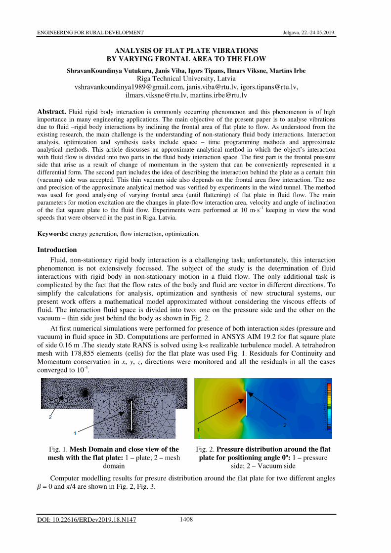
ENGINEERING FOR RURAL DEVELOPMENT Jelgava, 22.-24.05.2019. 1408 ANALYSIS OF FLAT PLATE VIBRATIONS BY VARYING FRONTAL AREA TO THE FLOW ShravanKoundinya Vutukuru, Janis Viba, Igors Tipans, Ilmars Viksne, Martins Irbe Riga Technical University, Latvia [email protected], [email protected], [email protected], [email protected], [email protected] Abstract. Fluid rigid body interaction is commonly occurring phenomenon and this phenomenon is of high importance in many engineering applications. The main objective of the present paper is to analyse vibrations due to fluid –rigid body interactions by inclining the frontal area of flat plate to flow. As understood from the existing research, the main challenge is the understanding of non-stationary fluid body interactions. Interaction analysis, optimization and synthesis tasks include space – time programming methods and approximate analytical methods. This article discusses an approximate analytical method in which the object’s interaction with fluid flow is divided into two parts in the fluid body interaction space. The first part is the frontal pressure side that arise as a result of change of momentum in the system that can be conveniently represented in a differential form. The second part includes the idea of describing the interaction behind the plate as a certain thin (vacuum) side was accepted. This thin vacuum side also depends on the frontal area flow interaction. The use and precision of the approximate analytical method was verified by experiments in the wind tunnel. The method was used for good analysing of varying frontal area (until flattening) of flat plate in fluid flow. The main parameters for motion excitation are the changes in plate-flow interaction area, velocity and angle of inclination of the flat square plate to the fluid flow. Experiments were performed at 10 m·s -1 keeping in view the wind speeds that were observed in the past in Riga, Latvia. Keywords: energy generation, flow interaction, optimization. Introduction Fluid, non-stationary rigid body interaction is a challenging task; unfortunately, this interaction phenomenon is not extensively focussed. The subject of the study is the determination of fluid interactions with rigid body in non-stationary motion in a fluid flow. The only additional task is complicated by the fact that the flow rates of the body and fluid are vector in different directions. To simplify the calculations for analysis, optimization and synthesis of new structural systems, our present work offers a mathematical model approximated without considering the viscous effects of fluid. The interaction fluid space is divided into two: one on the pressure side and the other on the vacuum – thin side just behind the body as shown in Fig. 2. At first numerical simulations were performed for presence of both interaction sides (pressure and vacuum) in fluid space in 3D. Computations are performed in ANSYS AIM 19.2 for flat sqaure plate of side 0.16 m .The steady state RANS is solved using k-ε realizable turbulence model. A tetrahedron mesh with 178,855 elements (cells) for the flat plate was used Fig. 1. Residuals for Continuity and Momentum conservation in x, y, z, directions were monitored and all the residuals in all the cases converged to 10 -4 . Fig. 1. Mesh Domain and close view of the mesh with the flat plate: 1 – plate; 2 – mesh domain Fig. 2. Pressure distribution around the flat plate for positioning angle 0º: 1 – pressure side; 2 – Vacuum side Computer modelling results for presure distribution around the flat plate for two different angles β = 0 and π/4 are shown in Fig. 2, Fig. 3. DOI: 10.22616/ERDev2019.18.N147
Transcript of ANALYSIS OF FLAT PLATE VIBRATIONS BY VARYING FRONTAL …
ENGINEERING FOR RURAL DEVELOPMENT Jelgava, 22.-24.05.2019.
1408
ANALYSIS OF FLAT PLATE VIBRATIONS
BY VARYING FRONTAL AREA TO THE FLOW
ShravanKoundinya Vutukuru, Janis Viba, Igors Tipans, Ilmars Viksne, Martins Irbe
Riga Technical University, Latvia
[email protected], [email protected], [email protected],
[email protected], [email protected]
Abstract. Fluid rigid body interaction is commonly occurring phenomenon and this phenomenon is of high
importance in many engineering applications. The main objective of the present paper is to analyse vibrations
due to fluid –rigid body interactions by inclining the frontal area of flat plate to flow. As understood from the
existing research, the main challenge is the understanding of non-stationary fluid body interactions. Interaction
analysis, optimization and synthesis tasks include space – time programming methods and approximate
analytical methods. This article discusses an approximate analytical method in which the object’s interaction
with fluid flow is divided into two parts in the fluid body interaction space. The first part is the frontal pressure
side that arise as a result of change of momentum in the system that can be conveniently represented in a
differential form. The second part includes the idea of describing the interaction behind the plate as a certain thin
(vacuum) side was accepted. This thin vacuum side also depends on the frontal area flow interaction. The use
and precision of the approximate analytical method was verified by experiments in the wind tunnel. The method
was used for good analysing of varying frontal area (until flattening) of flat plate in fluid flow. The main
parameters for motion excitation are the changes in plate-flow interaction area, velocity and angle of inclination
of the flat square plate to the fluid flow. Experiments were performed at 10 m·s-1
keeping in view the wind
speeds that were observed in the past in Riga, Latvia.
Keywords: energy generation, flow interaction, optimization.
Introduction
Fluid, non-stationary rigid body interaction is a challenging task; unfortunately, this interaction
phenomenon is not extensively focussed. The subject of the study is the determination of fluid
interactions with rigid body in non-stationary motion in a fluid flow. The only additional task is
complicated by the fact that the flow rates of the body and fluid are vector in different directions. To
simplify the calculations for analysis, optimization and synthesis of new structural systems, our
present work offers a mathematical model approximated without considering the viscous effects of
fluid. The interaction fluid space is divided into two: one on the pressure side and the other on the
vacuum – thin side just behind the body as shown in Fig. 2.
At first numerical simulations were performed for presence of both interaction sides (pressure and
vacuum) in fluid space in 3D. Computations are performed in ANSYS AIM 19.2 for flat sqaure plate
of side 0.16 m .The steady state RANS is solved using k-ε realizable turbulence model. A tetrahedron
mesh with 178,855 elements (cells) for the flat plate was used Fig. 1. Residuals for Continuity and
Momentum conservation in x, y, z, directions were monitored and all the residuals in all the cases
converged to 10-4
.
Fig. 1. Mesh Domain and close view of the
mesh with the flat plate: 1 – plate; 2 – mesh
domain
Fig. 2. Pressure distribution around the flat
plate for positioning angle 0º: 1 – pressure
side; 2 – Vacuum side
Computer modelling results for presure distribution around the flat plate for two different angles
β = 0 and π/4 are shown in Fig. 2, Fig. 3.
DOI: 10.22616/ERDev2019.18.N147

ENGINEERING FOR RURAL DEVELOPMENT Jelgava, 22.-24.05.2019.
1409
The following important conclusion can be drawn from the static pressure distribution for the flat
plate is that the vacuum side: the thin side just downstream of the plate along the entire boundary
region is approximately constant.
Fig. 3. Pressure distribution around the flat plate
at 45º in counter clock wise rotation.
Fig. 4. Pressure distribution for triangular
prism with leading vertex angle 30º
Additional 2D computation results for three different angled cross section prisms to check the
important conclusion for constant vacuum along the boundary closer to the body as constant is
verified. Some examples of pressure distributions are shown in Fig. 3-6.
Fig. 5. Pressure distribution for triangular prism
with leading vertex angle 45º
Fig. 6. Pressure distribution for triangular
prism with leading vertex angle 60º
1. Flat plate interaction model and method
The essence of the model in the case of flat plate body is described in Fig. 7.
For the pressure side forces F1 , F2, the theorem of the change in momentum of flow in the
differential form can be applied (1), (2) [1-4]:
;cos( )dm v dN dtβ⋅ ⋅ = ⋅
(1)
,co ( )sdm v dt dL Bβ ρ= ⋅ ⋅ ⋅ ⋅⋅
(2)
where dm – mass of the elemental volume of the flow stream, which rises at the velocity v
against the inclined surface;
β – the angle between the flow and the surface at the normal point of impact;
dN – the impact force in the direction of the normal surface of the elemental area;
t – time;
dL – the elemental length of the surface;
B – width of the object, which is constant in the case of a two-dimensional (2D cylinder)
task;
ρ – Density of air.
By integration of equation (1),(2) additional pressure and forces N1, N2 perpendicular to both
sides can be calculated from equations (3), (4).
( )22 ;1 1N A v cosρ β= ⋅ ⋅⋅
(3)
( )22 ,2 2 sinN A v ρ β= ⋅ ⋅⋅
(4)
where A1, A2 – area of sides.

ENGINEERING FOR RURAL DEVELOPMENT Jelgava, 22.-24.05.2019.
1410
Fig. 7. Model in the case of rectangle flat plate: L1, B – length of flat plate sides; L2 – thickness of
plate; A1, A2 – area of sides; N1, N2 – centre forces of additional pressure in frontal sides;
N3, N4 – centre forces of vacuum (thin) side; V – flow velocity
Vacuum (thin) side along the edge of the body is aproximately constant pressure. That is
proportional to the density ρ multiplied by the flow velocity square in the following forms (5), (6):
2 ;3 1N A v Cρ= ⋅ ⋅ ⋅ (5)
24 2 ,N A v Cρ= ⋅ ⋅ ⋅ (6)
where C – constant, to be found out experimentally or by computer modelling.
At the centre of plate O from equations (3) – (6) can be obtained two components of interaction
forces (7), (8):
3 32 cos( ) si
;n( )
H Bcos( ) sin( )
dFx v C
d
β βρ
β β+ ⋅
= − +
⋅
⋅ ⋅+
⋅ ⋅
(7)
( ) ( ) ( )2 32 L1 B sin( ) cos( ) .sin( ) cos( ) cos( )Fy v C d dρ β β β β β= ⋅ ⋅ ⋅ ⋅ ⋅ + ⋅ ⋅ + ⋅ − (8)
Here (Fig. 7.):
1 (cos( ) sin( )),H L dβ β= ⋅ + ⋅ 2
,1
Ld
L= (9)
where Fx – in the direction of x axis force component, named in fluid dynamics as Drag force;
Fy – parallel to y axis force component, named in fluid dynamics as Lifting force [5];
H – section height perpendicular to flow.
From Equation (7), (8) coefficient C is obtained as discussed below.
2. Model verification by 2D simulation
For coefficient C, 2D numerical simulations in SolidWorks flat plate drag interaction is
investigated.
From the fluid Dynamics analysis (pressure graph), the interaction force is constantly fluctuating
within certain limits, which depend on the angular β values: at smaller angle, the amplitude of the
fluctuations small and is greater at higher β values. Therefore, only the mean values of interactions are
analyzed here. Accordingly, part of interaction D1(β) as mentioned was found out by the step series
(10):
ENGINEERING FOR RURAL DEVELOPMENT Jelgava, 22.-24.05.2019.
1411
3 4 5
2
1( ) 3.7266204256 ( ) 1.5249241156366900458 ( ) 0.1013532598492 ( )
2.81293523749905363 ( ) 0.2823061 ( ) 1.5.
D β β β β
β β
= ⋅ − ⋅ − ⋅ +
− ⋅ + ⋅ + (10)
For (β = 0), that coefficient in equation (7) is C = 0.5, obtained from (10) and formula (7) can be
used in form (11), (12):
[ ]2 H B 2( ) ;Fx v Dρ β= − ⋅ ⋅ ⋅ ⋅
(11)
⋅+
⋅++=
)sin()cos(
)sin()cos(5.0)(2
33
ββββ
βd
dD
(12)
Accordingly, for (10), (11) Drag force coefficients DF1(β) and DF2(β) will be (13) (14):
1( ) 1( ) (cos( ) sin( )),DF D dβ β β β= ⋅ + ⋅ (13)
3 32( ) 0.5 (cos( ) sin( )) (cos( )) (sin( )) .DF d dβ β β β β= ⋅ + ⋅ + + ⋅ (14)
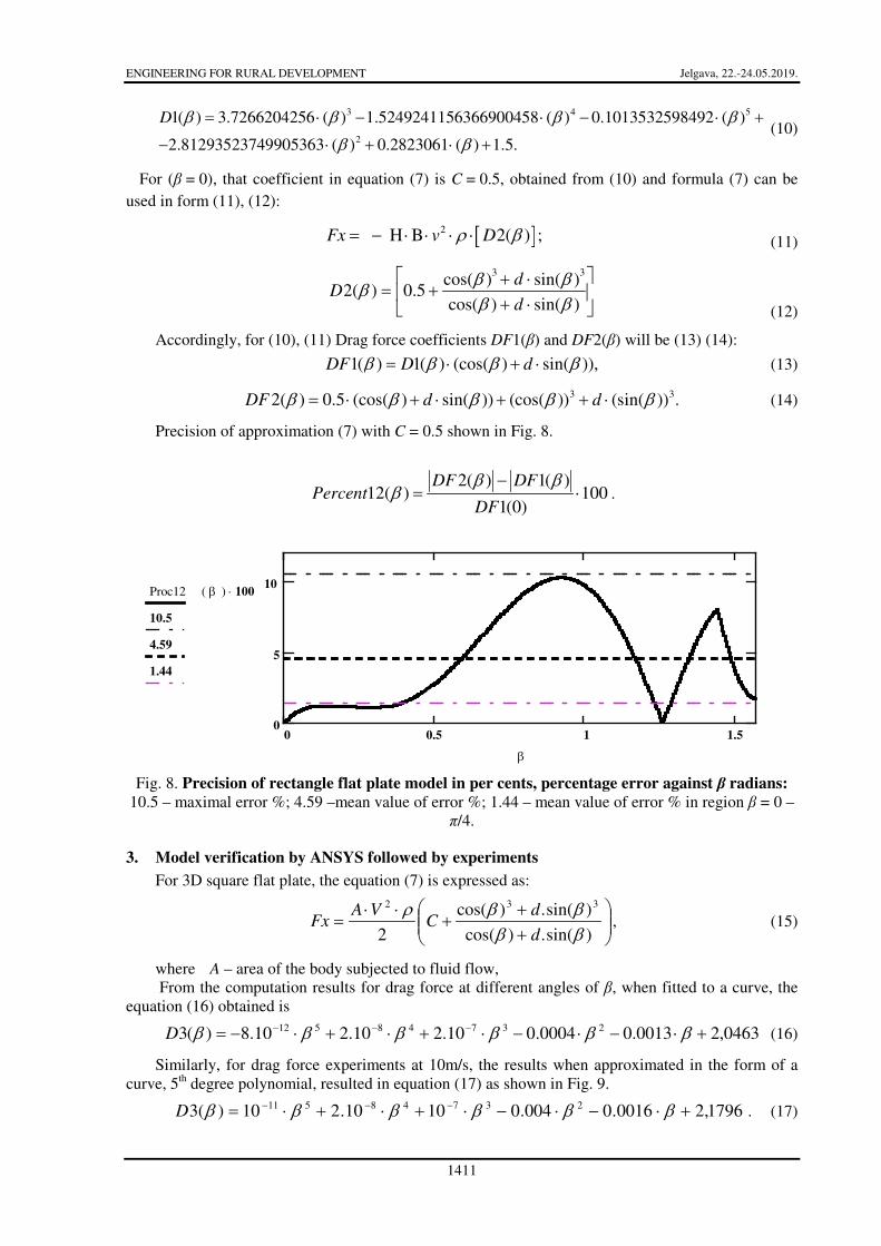
Precision of approximation (7) with C = 0.5 shown in Fig. 8.
2( ) 1( )
12( ) 1001(0)
DF DFPercent
DF
β ββ
−= ⋅ .
0 0.5 1 1.50
5
10Proc12 β( ) 100⋅
10.5
4.59
1.44
β
Fig. 8. Precision of rectangle flat plate model in per cents, percentage error against β radians:
10.5 – maximal error %; 4.59 –mean value of error %; 1.44 – mean value of error % in region β = 0 –
π/4.
3. Model verification by ANSYS followed by experiments
For 3D square flat plate, the equation (7) is expressed as:
++
+⋅⋅
=)sin(.)cos(
)sin(.)cos(
2
332
ββββρ
d
dC
VAFx , (15)
where A – area of the body subjected to fluid flow,
From the computation results for drag force at different angles of β, when fitted to a curve, the
equation (16) obtained is
0463,20013.00004.010.210.210.8)(3 23748512 +⋅−⋅−⋅+⋅+⋅−= −−− ββββββD (16)
Similarly, for drag force experiments at 10m/s, the results when approximated in the form of a
curve, 5th degree polynomial, resulted in equation (17) as shown in Fig. 9.
1796,20016.0004.01010.210)(3 23748511 +⋅−⋅−⋅+⋅+⋅= −−− ββββββD . (17)

ENGINEERING FOR RURAL DEVELOPMENT Jelgava, 22.-24.05.2019.
1412
From equation (15), calculating the interaction Force (Drag force) for the given geometry, the
value of constant C = 0.31 is obtained for β = 00. Thereby, the equation for plate in 3D for motion
analysis at β = 0º is given by equation (18). The value 1.31 is taken for co-efficient of interaction. It
was observed that the maximum error measured for Drag force at β = 0º, in computations and
experiments was ~6 % as analysed from Fig. 9. Additional information from the simulations is given
in Fig. 10, Fig. 11.
}))sin(.5.05.0({].)))sin(.5.05.0([(..).31.1( 2 xptVsignxptVHBxbcxxm &&&&& +−+−−−−= ρ (18)
Fig. 9. Drag force experiment results for flat plate at velocity 10 m·s-1
, β degrees
Fig. 10. Vorticity contour for flat plate at
β = 0º: 1 – flat plate; 2 – flow separation (vortex
street formation)
Fig. 11. Coefficient of Lift flow for (β = 0º)
as a function of time (varies within a
large range around zero)
4. Vibration analysis by Mathcad and Working Model 2D
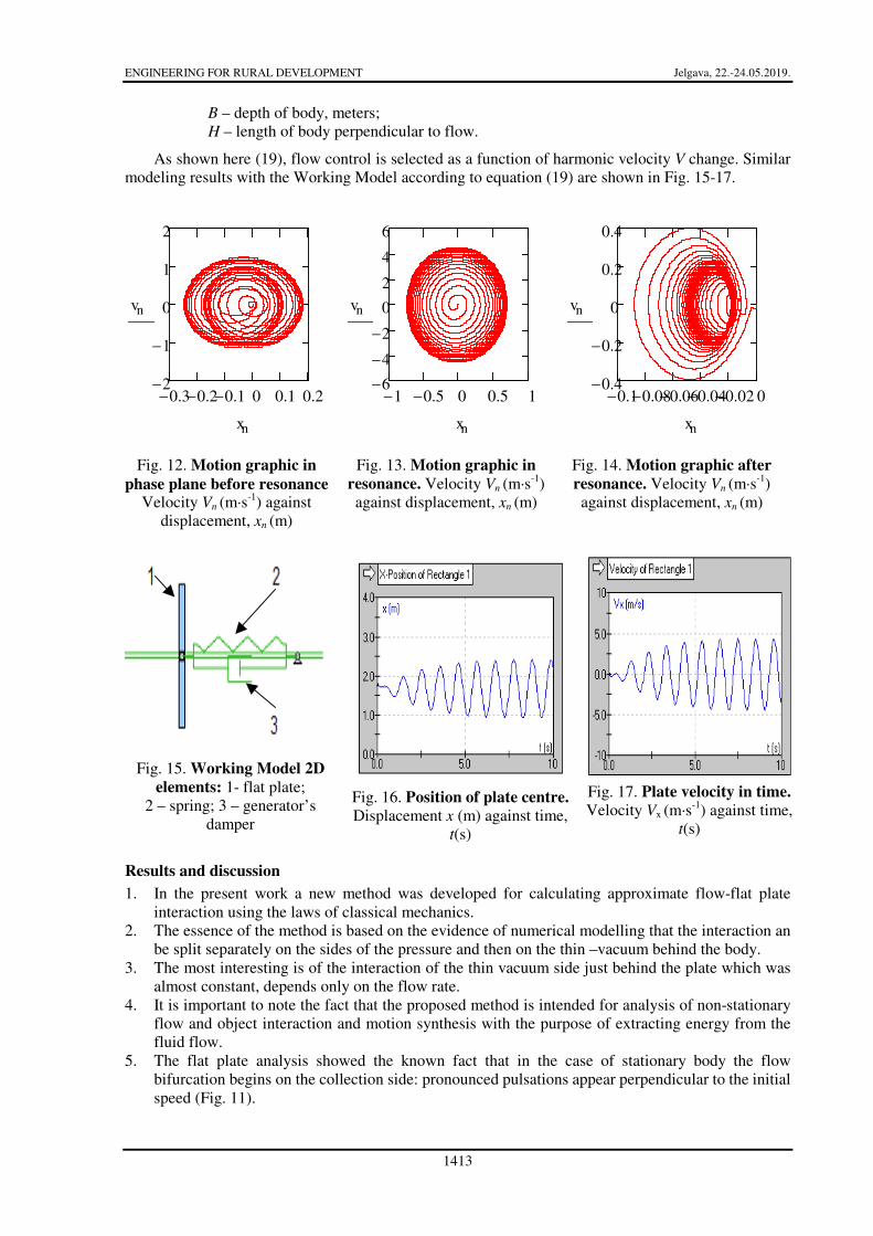
An example of a flat plate motion analysis in 2D space by Mathcad is shown in Fig. 12-14. The
system considered consists of the mass of the plate, the spring, the energy generator and the flow,
according to the equation (19),
}{ xptVsignxptVHBxbcxxm &&&&& +−⋅+⋅−⋅⋅−−−= ))sin(5.05.0(])))sin(5.05.0(([)5.1(2ρ (19)
where m – mass, kg;
x – displacement, meters;
x - velocity, m·s-1
;
c – stiffness of spring;
b – linear generator damping;
1.5 – co-efficient of interaction;
V – flow velocity, m·s-1
;
p – velocity control actions harmonic angular frequency;
t – time, seconds;
ENGINEERING FOR RURAL DEVELOPMENT Jelgava, 22.-24.05.2019.
1413
B – depth of body, meters;
H – length of body perpendicular to flow.
As shown here (19), flow control is selected as a function of harmonic velocity V change. Similar
modeling results with the Working Model according to equation (19) are shown in Fig. 15-17.
Fig. 12. Motion graphic in
phase plane before resonance Velocity Vn (m·s
-1) against
displacement, xn (m)
Fig. 13. Motion graphic in
resonance. Velocity Vn (m·s-1
)
against displacement, xn (m)
Fig. 14. Motion graphic after
resonance. Velocity Vn (m·s-1
)
against displacement, xn (m)
Fig. 15. Working Model 2D
elements: 1- flat plate;
2 – spring; 3 – generator’s
damper
Fig. 16. Position of plate centre.
Displacement x (m) against time,
t(s)
Fig. 17. Plate velocity in time.
Velocity Vx (m·s-1
) against time,
t(s)
Results and discussion
1. In the present work a new method was developed for calculating approximate flow-flat plate
interaction using the laws of classical mechanics.
2. The essence of the method is based on the evidence of numerical modelling that the interaction an
be split separately on the sides of the pressure and then on the thin –vacuum behind the body.
3. The most interesting is of the interaction of the thin vacuum side just behind the plate which was
almost constant, depends only on the flow rate.
4. It is important to note the fact that the proposed method is intended for analysis of non-stationary
flow and object interaction and motion synthesis with the purpose of extracting energy from the
fluid flow.
5. The flat plate analysis showed the known fact that in the case of stationary body the flow
bifurcation begins on the collection side: pronounced pulsations appear perpendicular to the initial
speed (Fig. 11).
1− 0.5− 0 0.5 16−
4−
2−
0
2
4
6
vn
xn
0.3− 0.2− 0.1− 0 0.1 0.22−
1−
0
1
2
vn
xn
0.1− 0.08− 0.06− 0.04− 0.02− 00.4−
0.2−
0
0.2
0.4
vn
xn

ENGINEERING FOR RURAL DEVELOPMENT Jelgava, 22.-24.05.2019.
1414
Conclusions
1. The method developed in the thesis allows performing tasks of analysis, optimization and
synthesis in the interaction of objects with fluids in a simplified way.
2. This means there is no need to use time-space intensive computing programs.
3. The developed theory can be used in calculations of flying or diving robot systems, as well as in
the extraction of energy from the fluid flow.
References
[1] Clancy L.J., Aerodynamics. London: Publishing by Pitman, 1975. 610p.
[2] Meriam J. L., Kraige L.G., Bolton J. N. Engineering Mechanics: Dynamics, 8th Edition, Wiley,
2015. 736 pp.
[3] Goldstein H., Poole C.P., Safko J.L. Classical Mechanics. Third Edition, Addison Wesley,
2000.625 p.
[4] Sears W.R. Introduction to Theoretical Aerodynamics and Hydrodynamics, American Institute of
Aeronautics and Astronautics, Reston, VA, 2011. 203p.
[5] Hoerner S. F. Fluid-Dynamic Drag.1965.
[6] Vība J., Beresņevičs V., Noskovs S., Irbe M. Investigations of Rotating Blade for Energy
Extraction from Fluid Flow. Vibroenginesering PROCEDIA, vol. 8, 2016. pp. 312-315.
[7] Flat Plate Drag [online][16.02.2019] Available at:
https://www.engineersedge.com/fluid_flow/rectangular_flat_plate_drag_14036.htm
[8] Drag force on a flat plate [online][16.02.2019] Available at:
https://physics.stackexchange.com/questions/138166/drag-force-on-a-flat-plate.