ANALYSIS OF FACTORS AFFECTING FARMERS’ WILLINGNESS TO ...
113
University of Tennessee, Knoxville University of Tennessee, Knoxville TRACE: Tennessee Research and Creative TRACE: Tennessee Research and Creative Exchange Exchange Masters Theses Graduate School 5-2011 ANALYSIS OF FACTORS AFFECTING FARMERS’ WILLINGNESS TO ANALYSIS OF FACTORS AFFECTING FARMERS’ WILLINGNESS TO ADOPT SWITCHGRASS PRODUCTION IN THE SOUTHERN UNITED ADOPT SWITCHGRASS PRODUCTION IN THE SOUTHERN UNITED STATES AND AN EXCEL SPREADSHEET-BASED DECISION TOOL STATES AND AN EXCEL SPREADSHEET-BASED DECISION TOOL FOR POTIENTIAL SWITCHGRASS PRODUCERS FOR POTIENTIAL SWITCHGRASS PRODUCERS Donald Joshua Qualls [email protected] Follow this and additional works at: https://trace.tennessee.edu/utk_gradthes Recommended Citation Recommended Citation Qualls, Donald Joshua, "ANALYSIS OF FACTORS AFFECTING FARMERS’ WILLINGNESS TO ADOPT SWITCHGRASS PRODUCTION IN THE SOUTHERN UNITED STATES AND AN EXCEL SPREADSHEET-BASED DECISION TOOL FOR POTIENTIAL SWITCHGRASS PRODUCERS. " Master's Thesis, University of Tennessee, 2011. https://trace.tennessee.edu/utk_gradthes/933 This Thesis is brought to you for free and open access by the Graduate School at TRACE: Tennessee Research and Creative Exchange. It has been accepted for inclusion in Masters Theses by an authorized administrator of TRACE: Tennessee Research and Creative Exchange. For more information, please contact [email protected].
Transcript of ANALYSIS OF FACTORS AFFECTING FARMERS’ WILLINGNESS TO ...

University of Tennessee, Knoxville University of Tennessee, Knoxville
TRACE: Tennessee Research and Creative TRACE: Tennessee Research and Creative
Exchange Exchange
Masters Theses Graduate School
5-2011
ANALYSIS OF FACTORS AFFECTING FARMERS’ WILLINGNESS TO ANALYSIS OF FACTORS AFFECTING FARMERS’ WILLINGNESS TO
ADOPT SWITCHGRASS PRODUCTION IN THE SOUTHERN UNITED ADOPT SWITCHGRASS PRODUCTION IN THE SOUTHERN UNITED
STATES AND AN EXCEL SPREADSHEET-BASED DECISION TOOL STATES AND AN EXCEL SPREADSHEET-BASED DECISION TOOL
FOR POTIENTIAL SWITCHGRASS PRODUCERS FOR POTIENTIAL SWITCHGRASS PRODUCERS
Donald Joshua Qualls [email protected]
Follow this and additional works at: https://trace.tennessee.edu/utk_gradthes
Recommended Citation Recommended Citation Qualls, Donald Joshua, "ANALYSIS OF FACTORS AFFECTING FARMERS’ WILLINGNESS TO ADOPT SWITCHGRASS PRODUCTION IN THE SOUTHERN UNITED STATES AND AN EXCEL SPREADSHEET-BASED DECISION TOOL FOR POTIENTIAL SWITCHGRASS PRODUCERS. " Master's Thesis, University of Tennessee, 2011. https://trace.tennessee.edu/utk_gradthes/933
This Thesis is brought to you for free and open access by the Graduate School at TRACE: Tennessee Research and Creative Exchange. It has been accepted for inclusion in Masters Theses by an authorized administrator of TRACE: Tennessee Research and Creative Exchange. For more information, please contact [email protected].

To the Graduate Council:
I am submitting herewith a thesis written by Donald Joshua Qualls entitled "ANALYSIS OF
FACTORS AFFECTING FARMERS’ WILLINGNESS TO ADOPT SWITCHGRASS PRODUCTION IN
THE SOUTHERN UNITED STATES AND AN EXCEL SPREADSHEET-BASED DECISION TOOL FOR
POTIENTIAL SWITCHGRASS PRODUCERS." I have examined the final electronic copy of this
thesis for form and content and recommend that it be accepted in partial fulfillment of the
requirements for the degree of Master of Science, with a major in Agricultural Economics.
Kimberly L. Jensen, Major Professor
We have read this thesis and recommend its acceptance:
Burton C. English, Daniel G. de la Torre Ugarte
Accepted for the Council:
Carolyn R. Hodges
Vice Provost and Dean of the Graduate School
(Original signatures are on file with official student records.)
ANALYSIS OF FACTORS AFFECTING FARMERS’ WILLINGNESS TO ADOPT
SWITCHGRASS PRODUCTION IN THE SOUTHERN UNITED STATES
ANDAN EXCEL SPREADSHEET-BASED DECISION TOOL FOR POTIENTIAL
SWITHGRASS
PRODUCERS
A Thesis
Presented for the Master of Science Degree
The University of Tennessee, Knoxville
Donald Joshua Qualls
May 2011

ii
ABSTRACT
The increased need for and scarcity of hydrocarbon energy pushes the search and extraction of
reserves toward more technically difficult deposits and less efficient forms of hydrocarbon energy. The
increased use of hydrocarbons also predicates the increased emission of detrimental chemicals in our
surrounding environment. For these reasons, there is a need to find feasible sources of renewable energy
that could prove to be more environmentally friendly.
One possible source that meets these criteria is biomass, which in the United States is the largest
source of renewable energy as it accounts for over 3 percent of the energy consumed domestically and is
currently the only source for liquid renewable transportation fuels. Continued development of biomass
as a renewable energy source is being driven in large part by the Energy Independence and Security Act
of 2007 that mandates that by 2022 at least 36 billion gallons of fuel ethanol be produced, with at least
16 billion gallons being derived from cellulose, hemi-cellulose, or lignin. However, the production of
biomass has drawbacks. The market for cellulosic bio-fuel feedstock is still under development, and
being an innovative technique, there is a lack of production knowledge on the side of the producer.
Some studies have been conducted that determine farmers’ willingness to produce switchgrass,
however, they have been limited in geographic scope and additional research is warranted considering a
broader area. Also, there have been production decision tools aimed at bio-mass, but these have either
not been aimed at switchgrass specifically or have been missing key costs such as those incurred in
storage. The overall objectives of this study are: 1.) to analyze the willingness of producers in the
southeastern United States to plant switchgrass as a biofuel feedstock, 2.) to estimate the area of
switchgrass they would be willing to plant at different switchgrass prices, 3.) to evaluate the factors that
influence a producer’s decision to convert acreage to switchgrass, and 4.) to present a spreadsheet-based
decision tool for potential switchgrass producers.
iii
Table of Contents Part 1: Introduction ......................................................................................................................................1
Introduction ..................................................................................................................................................2
Objectives ....................................................................................................................................................5
References ....................................................................................................................................................7
Part 2: Analysis of Factors Affecting Farmers’ Willingness to Adopt Switchgrass Production in the Southeastern United States ..............................................................................................................9
Introduction ................................................................................................................................................10
Objectives ..................................................................................................................................................13
Review of Literature ..................................................................................................................................14
Empirical Adoption Studies ...........................................................................................................14
Farmer Characteristics .......................................................................................................14
Farm Characteristics ..........................................................................................................17
Switchgrass Survey Studies ...........................................................................................................18
Conceptual Framework ..............................................................................................................................20
Methodology ..............................................................................................................................................21
Statistical Analysis .........................................................................................................................21 Hypothesized Effects .....................................................................................................................24
Data ................................................................................................................................................33
Results ........................................................................................................................................................34
Tobit Model with Sample Selection ..............................................................................................34
Probit Selection Equation for INTEREST .....................................................................................35
Farm and Farmer Variables ...........................................................................................................35 Opinion Variables ..........................................................................................................................36
Tobit Regression for the Share of Acres Producers are Willing to Convert to Switchgrass .........37
Conclusions ................................................................................................................................................38
References ..................................................................................................................................................41
Appendix A: Tables ...................................................................................................................................46 Appendix B: Survey ...................................................................................................................................56
Part 3: An Excel Spreadsheet-Based Decision Tool for Potential Switchgrass Producers . 65 Introduction....................................................................................................................................................................66
Objective ....................................................................................................................................................68
Literature Review.......................................................................................................................................69
Case Study .................................................................................................................................................71 Methods......................................................................................................................................................71

iv
Input-Output Worksheet ................................................................................................................71
Input section ...................................................................................................................................72
Output Section ...............................................................................................................................73 Cash Flow Sheet ............................................................................................................................75
Cost Distribution ............................................................................................................................76
Yearly Cash Flow ..........................................................................................................................77 Accumulated Cash Flow ................................................................................................................77
Planting and Establishment Sheet ..................................................................................................78
Stand Maintenance .........................................................................................................................84 Harvest Sheet .................................................................................................................................85
Transportation Worksheet ..............................................................................................................90
Storage Worksheet .........................................................................................................................93 Biomass Harvested Worksheet ......................................................................................................96
Conclusions ................................................................................................................................................97
References ..................................................................................................................................................98 Part 4: Conclusions ..................................................................................................................................101 Conclusions ..............................................................................................................................................102 Vita ...........................................................................................................................................................105

v
LIST OF TABLES Table A.1. Farm and farmer demographics for the sample .................................................................47
Table A.2. Farm and farmer demographics for the sample cont. .......................................................48
Table A.3. Familiarity and interest in growing switchgrass as an energy crop ...................................49
Table A.4. Farmer characteristics ........................................................................................................50
Table A.5. Hay equipment demographics ...........................................................................................51
Table A.6. Farmer concerns about risk and loss ..................................................................................52
Table A.7. Farm organization ..............................................................................................................53
Table A.8. Variable means and estimated values ................................................................................54
Table A.9. Estimated Tobit model with sample selection ...................................................................55

vi
LIST OF FIGURES Figure 1. The input section of the input-output sheet ........................................................................73
Figure 2. The output section of the input-output sheet .....................................................................74
Figure 3. The per acre section of the cash flow sheet. .....................................................................76
Figure 4. The cost distribution sheet. ...............................................................................................77
Figure 5. The per acre yearly cash flow diagram. ............................................................................77
Figure 6. The accumulated per acre cash flow diagram. ..................................................................78
Figure 7. NPV sensitivity Analysis and NPV Breakdown Price .......................................................78
Figure 8. The general data, labor, and travel costs subsections of the planting and establishment sheet. ..................................................................................................................................80
Figure 9. the equipment costs subsection of the planting and establishment sheet ..........................82
Figure 10. The supplies costs and the total cost subsections of the planting and establishment sheet.............................................................................................................................................83
Figure 11. The stand maintenance sheet. ............................................................................................85 Figure 12. The general input, labor, and travel costs subsections for the harvest sheet .....................86 Figure 13. The equipment costs subsections of the harvest sheet .......................................................89 Figure 14. The harvest costs per ton by year .......................................................................................90 Figure 15. The general data, labor costs, and equipment costs subsections of the transportation sheet.
............................................................................................................................................92 Figure 16. The yearly transportation costs of the transportation worksheet. ......................................93 Figure 17. The general data, bailing method, storage time, and storage method subsections of the
storage sheet .......................................................................................................................94 Figure 18. The dry matter loss schedule of the storage worksheet .....................................................95 Figure 19. The storage costs per year in the storage sheet ..................................................................96 Figure 20. The biomass harvested Sheet .............................................................................................96

Part 1: Introduction

2
Introduction
Much of the energy used in the industrialized world comes from fossil fuels such as coal,
petroleum, and natural gas. Although these chemicals are still being created underground by the
forces of heat and pressure, they are being consumed in quantities far exceeding the formation of
new reserves. This increased need for and scarcity of hydrocarbon energy pushes the search and
extraction of reserves toward more technically difficult deposits and less efficient forms of
hydrocarbon energy. The increased use of hydrocarbons also predicates the increased emission
of detrimental chemicals in our surrounding environment. For these reasons, there is a need to
find feasible sources of renewable energy that could prove to be more environmentally friendly.
One of these sources of renewable energy that has been the subject of much research is
biomass. Biomass is material derived from living or once living organisms such as herbaceous
and woody plant constituents and animal wastes that can be used to make solid, liquid, and
gaseous fuels. It is the largest source of renewable energy accounting for over 3 percent of the
energy consumed domestically and is also currently the only source for liquid renewable fuels
used in transportation (Perlack et al. 2005).
Of the possible ways to take advantage of direct and indirect energy from the sun,
biomass use is promising because it is compatible with current technologies and it can be stored
without technical problems which allows for its energy to be used when needed (Kaltschmitt
1994). Biomass could prove to be a clean energy source as it absorbs the carbon that it releases
during combustion from the atmosphere, potentially making it carbon neutral.
The source of biomass that will be the focus of this study is switchgrass. Switchgrass is a
C4 carbon fixation perennial warm season grass (Lewandowski et al. 2003). The perennial nature
of switchgrass gives it the advantage over annual crops for cellulosic biomass because it does not

3
have fixed annual establishment requirements. Its native habitat includes the prairies, open
ground and wooded areas, marshes, and pinewoods of much of North America east of the Rocky
Mountains and south of 55°N latitude (Stubbendieck et al. 1991). There are two distinct
geographic varieties or ecotypes of switchgrass: lowland and highland (Porter 1966; Brunken
and Estes 1975). Lowland types can be found on flood plains and other areas that may be subject
to inundation and upland types can typically be found in areas that have a low potential to flood
(Vogel 2004). Lowland types tend to be taller, coarser, and show the ability to grow more rapidly
than upland types (Vogel 2004).
There are many benefits that could be realized from the planting of switchgrass as a
biomass feedstock for fuel. Switchgrass has the capability to show high yields on soil that, due to
low availability of nutrients or water, would not lend itself to the cultivation of conventional
crops (Lewandowski et al. 2003). Being a native species, it also has a natural tolerance to pest
and diseases and can be grown successfully throughout a large portion of the United States with
minimal fertilizer applications (Jensen et al. 2007), which would be cost efficient and less
disruptive to the surrounding environment. Switchgrass has the capability to show high yields on
soil that, due to low availability of nutrients or water, would not lend itself to the cultivation of
conventional crops (Lewandowski et al. 2003), meaning that the grass could add profitability to
land that may not be economically useful otherwise. It has the positive attribute of reducing
erosion due to its extensive root system and canopy cover (Ellis 2006) and shows the potential
ability to reduce the buildup of CO2 by being a feedstock for a cleaner burning fuel than fossil
fuels and through soil carbon sequestration due it is being a deep rooted crop (Ma et al.2000).
Growing switchgrass as a biomass feedstock crop would add diversity to the American
crop mix. Introducing a new crop, like switchgrass, into a two crop rotation such as the corn-

4
soybean rotation that dominates the Corn Belt can help alleviate pest buildups that demand the
increased use of pesticides (Janick et al. 1996). Additionally, the introduction of new crops into
agricultural production can increase and protect farm income by diversifying farm products,
hedging risks, and expanding markets and can also act as a catalyst for rural economic
development by creating locally based processing and packaging industries (Janick et al. 1996).
Despite the potential benefits that could be realized from the planting of switchgrass,
there are significant obstacles to overcome. Several factors would have to be taken into
consideration before a bio-refinery that utilizes switchgrass to produce ethanol could be
established in a given area. Because of the high cost associated with the transportation of
biomass from switchgrass, the area from which a bio-refinery would feasibly be able to draw
feedstock would need to be small, preferably within a 30 mile radius (Mitchell, Vogel, and
Sarath 2008). This means that it would have to be determined if the local farmers would be
willing to devote sufficient acreage to switchgrass to meet the needs of the bio-refinery. This
willingness will be a function of numerous factors including biomass feedstock profits,
variability of profits, and correlation of profits relative to traditional crop profits (Larson et al.
2005).
The large scale production of switchgrass as a bio-energy feedstock is still in the
developmental stage. Consequently, a lack of an established market and of knowledge exists
both on the part of the producer pertaining to the costs and activities associated with its
production and on the part of the researcher pertaining to farmer’s willingness to produce and
attitudes toward switchgrass. While some studies have focused on factors that determine
farmers’ willingness to produce switchgrass and their general attitudes toward switchgrass and
its production (e.g. Jensen et al. 2007; Bransby 1998; Wen et al. 2005), these studies have been

5
limited in geographic scope and additional research is warranted that considers a broader
geographical area and different variables in order to gain a more complete understanding of how
producers view biomass feedstock production.
Knowledge of where switchgrass is likely to be adopted and the factors that are involved
in the producers’ decisions to adopt are of critical importance to understanding the potential
development of switchgrass as an energy feedstock at a market level. Additionally, with
switchgrass being a new crop, many producers may not be familiar with the production costs
associated with growing switchgrass. An understanding of these costs is crucial in the producers’
decisions of if and to what extent they would be willing to produce switchgrass. That stated, a
financial decision tool would be of assistance to producers in making these production decisions.
Objectives
The overall objectives of this study are: 1.) to analyze the willingness of producers in the
southeastern United States to plant switchgrass as a biofuel feedstock, 2.) to estimate the area of
switchgrass they would be willing to plant at different switchgrass prices, 3.) to evaluate the
factors that influence a producer’s decision to convert acreage to switchgrass, and 4.) to present a
spreadsheet-based decision tool for potential switchgrass producers.
This thesis is organized into two major sections. The first section is a paper that focuses
on the factors pertaining to farmers’ interest in planting switchgrass and those that are associated
with their likelihood and the extent to which they would be willing to produce switchgrass given
different plant gate prices. To accomplish this, a Tobit specification model with a binary sample
selection rule will be used. The binary sample selection rule will be used to analyze the

6
producers’ interests in growing switchgrass and the Tobit model is used to estimate acreage
adoption in response to switchgrass prices and other variables if the producer shows interest in
growing switchgrass.
The second section of this thesis is a paper that describes and documents an interactive
producer decision tool. This tool is an excel workbook that contains an intereactive switchgrass
budget. The tool provides the user with detailed information on the costs incurred in each stage
of a switchgrass operation in each year of its duration, which, for the purposes of this analysis,
will be 10 years. The decision tool is broken down into 13 different worksheets, including:
welcome worksheet
tutorial worksheet
input-output worksheet
cash flow worksheet
cost distribution worksheet
yearly cash flow worksheet
accumulated cash flow
planting and establishment worksheet
7
References
Bransby, D. I. “Interest Among Alabama Farmers in Growing Switchgrass for Energy.” 1998.
Paper presented at BioEnergy '98: Expanding Bioenergy Partnerships, MadisonWI, Oct.
4-8.
Brunken J.N., Estes J.R. 1975. “Cytological and morphological Variationin Panicum virgatum
L.”The Southwestern Naturalist 19(4):379–385
Ellis, P. 2006. “Evaluation of Socioeconomic Characteristics Of Farmers Who Choose to Adopt
a New Type of Crop and Factors That Influence the Decision to Adopt Switchgrass for
Energy Production.” M.S. Thesis, Department of Agricultural and Resource Economics.
The University of Tennessee, Knoxville.
Janick, J., M.G. Blase, D.L. Johnson, G.D. Joliffe, and R.L. Myers. 1996. DiversifyingU.S. crop
production. P. 98-108. In: J. Janick (ed.), Progress in new crops. ASHS Press,Alexandria,
VA.
Jensen, K., C. D. Clark, P. Ellis, B. English, J. Menard, M. Walsh, and D. L. T. Ugarte. 2007.
“Farmer Willingness to Grow Switchgrass for Energy Production.” Biomass & Bioenergy
31:773-781.
Kaltschmitt, M. 1994. “The benefits and costs of energy from biomass in Germany.” Biomass
and Bioenergy 6(5):329-337.
Larson, J., B. English, C. Hellwinckel, D. Ugarte. 2005. “A Farmer Evaluation of Conditions
under Which Farmers Will Supply Biomass Feedstocks for Energy Production.” Paper
presented at the American Agricultural Economics Association Annual Meeting,
Providence RI, July 24-27.

8
Lewandski, I., J. M. O. Scurlock, E. Lindvall, and M. Chirstou. 2003. “The Development of
Perennial Rhizomatous Grasses as Energy Crops in the U. S. and Europe.” Biomass &
Bioenergy 25(4):335-361.
Ma, Z., C. Wood, and D. Bransby. 2000. “Carbon Dynamics Subsequent to Switchgrass
Establishment.” Biomass and Bioenergy 18:93-104.
Mitchell, R., K. Vogel, and G. Sarath. 2008. “Managing and Enhancing Switchgrass as a
Bioenergy Feedstock.” Biofuels, Bioproducts, and Biorefining 2:530-539.
Perlack, R. D., L. L. Wright, A. F. Turhollow, L. R. Graham , B. J. Stokes, and D. C. Erbach.
2005. “Biomass as Feedstock for a Bioenergy and Bioproducts Industry: the Technical
Feasibility of a Billion-Ton Annual Supply.” U.S. Department of Agriculture and U. S.
Department of Energy, Oak Ridge TN, April.
Porter, C.L. 1966. “An Analysis of Variations between Upland and Lowland Switchgrass in
Central Oklahoma.” Ecology 47:980-992.
Stubbendieck, J., S. L. Hatch, and C. H. Butterfield. 1992. “North American Range Plants.”
Fourth edition. University ofNebraska Press, Lincoln, Nebraska, USA.
Wen, Z., J. Ignosh, D. Parrish, J. Stowe, and B. Jones. 2005. “Identifying Farmers’ Interest in
Growing Switchgrass for Bio-energy in Southern Virginia.” Journal of Extension
47(4):5RIB7.
Vogel K.P. 2004.“Switchgrass”. In: Moser L.E., Burson B.L. and Sollenberger L.E. “Warm-
Season (C4) Grasses” American Society of Agronomy pp.561–588.

9
Part 2: Analysis of Factors Affecting Farmers’ Willingness to Adopt Switchgrass
Production in the Southern United States
10
Introduction
In the United States, biomass is the largest source of renewable energy accounting for
over 3 percent of the energy consumed domestically and is at present the only source for liquid,
renewable, transportation fuels (Perlack et al. 2005). The continued development of biomass as a
renewable energy source is being driven in large part by the Energy Independence and Security
Act of 2007 (EISA). The EISA is an energy policy law that mainly deals with increasing energy
efficiency and the availability of energy from biomass. The Act included three key provisions:
Corporate Average Fuel Economy (CAFE)Standards, Appliance and Lighting Efficiency
Standards, andRenewable Fuel Standard (RFS) (Sissine 2007). The Renewable Fuel Standard
mandates that by 2022 at least 36 billion gallons of ethanol for fuel be produced in the United
States, with at least 16 billion gallons being ethanol that is derived from cellulose, hemi-
cellulose, or lignin (U.S. Congress 2007).While EISA calls for increased production of
cellulosic-based fuels, the market for cellulosic-based fuels is still under development.
Development of a cellulosic-based fuel industry will rely not only on construction and operation
of conversion facilities, but also reliable, cost-efficient, and environmentally sustainable
cellulosic feedstock sources.
Several potential reasons for promoting the production of cellulosic ethanol in favor of
ethanol from cornstarch exist. Corn, which also has use as animal feed and human consumption,
will not be grown in sufficient quantities to meet the feedstock demand for fuel ethanol and is
not likely to displace current transportation fuels to a significant extent (Hahn-hagerdal et al.
2006, Lynd 1991). Because cellulosic fuels are not based upon a human or animal feed source,
cellulosic feedstock development would likely create minimal market pressure on food or animal
feed markets. Environmental benefits relative to the production of corn based ethanol may

11
accrue from production of cellulosic ethanol. Some perennial cellulosic energy crops have the
potential for reduced erosion due to being deep rooted plants and to require less chemical
applications than traditional row crops such as corn (Bransby)In addition, the production of
cellulosic ethanol is likely to show a higher reduction in green house gases than would the
production of corn based ethanol (Wang 2008).
Of the possible ways to take advantage of direct and indirect energy from the sun,
biomass use is promising, because it is compatible with current technologies and it can be stored
without technical problems which allows for its energy to be used when needed (Kaltschmitt
1994). Biomass could prove to be a clean energy source as it absorbs the carbon that it releases
during combustion from the atmosphere, potentially making it carbon neutral.
Approximately 19 years ago, The Bio-energy Feedstock Program based at Oak Ridge
National Laboratory concluded that more emphasis was needed on developing herbaceous bio-
energy crops that could “combine close compatibility of crop management strategies with
existing farming practices, generate cash flow from annual returns from harvested biomass, and
have positive environmental impacts on American farmlands”(McLaughlin and Kszos 2004
p.516). One crop that meets these criteria is switchgrass (Panicum vergatum). Switchgrass is a
C4 carbon fixation perennial warm season grass (Lewandowski et al. 2003). Native habitat
includes the prairies, open ground, open woods, marshes, and pinewoods of much of North
America east of the Rocky Mountains and south of 55°N latitude (Stubbendieck et al. 1991).
Several advantages to planting switchgrass as a biomass feedstock exist. Switchgrass has
a natural tolerance to pest and diseases and can be grown successfully throughout a large portion
of the United States with minimal fertilizer applications (Jensen et al. 2007). Requiring low
amounts of fertilizer and pesticide per acre is cost efficient and less disruptive to the surrounding
12
environment. Switchgrass has the capability to show high yields on soil that, due to low
availability of nutrients or water, would not lend itself to the cultivation of conventional crops
(Lewandowski et al. 2003), meaning that the grass could add profitability to land that may not be
economically useful otherwise. Switchgrass has the positive attribute of reducing erosion due to
its extensive root system and canopy cover (Ellis 2006), and has the potential ability to reduce
the buildup of CO2 by being a feedstock for a cleaner burning fuel than fossil fuels and by soil
carbon sequestration due it is being a deep rooted crop (Ma et al.2000).
Growing switchgrass as a biomass feedstock crop would add diversity to the American
crop mix. Diversification of cropping systems brings with it the possibility of many benefits.
Introducing a new crop, like switchgrass, into a two crop rotation such as the corn-soybean
rotation that dominates the Corn Belt can help alleviate pest buildups that demand the increased
use of pesticides (Janick et al. 1996). Additionally, the introduction of new crops into
agricultural production can increase and protect farm income by diversifying farm products,
hedging risks, and expanding markets and can also act as a catalyst for rural economic
development by creating locally based processing and packaging industries (Janick et al. 1996).
For cellulosic ethanol to be produced in sufficient quantities to have a significant impact
on the mix of energy inputs used in the United States, the large scale production of dedicated
energy crops will be required. However, a major hurdle to overcome is the lack of an established
market for cellulosic bio-mass feedstock. For a cellulosic feedstock market to develop producers
will have to be willing to plant dedicated energy crops on a massive scale and cellulosic ethanol
refineries will have to be available to purchase and convert the biomass to fuel. For instance, a
50 million gallon per year ethanol plant will require 464,253 short tons of feedstock if it is
assumed that 107.7 gallons of ethanol can be produced from one ton of feedstock ( Lynd 1996).

13
The EISA requires 16 billion gallons, and using 50 million gallon plants as an example, it means
approximately 320 plants would be required. These 320 plants would require roughly
148,561,000 tons of switchgrass to meet production goals. Because of the high cost associated
with the transportation of biomass the area from which a bio-refinery would feasibly be able to
draw feedstock would need to be small, preferably within a 30 mile radius (Mitchell, Vogel, and
Sarath 2008). Thus it would be critically important to determine if local producers would be
willing to devote sufficient acreage to cellulosic feedstock to meet the needs of the bio-refinery.
This willingness to grow cellulosic feed stock will be a function of numerous factors including
the amount and variability of feedstock profits and the relationship of feedstock profits relative to
traditional crop profits (Larson et al. 2005).
Most studies pertaining to switchgrass have focused on breeding, conversion
technologies, and logistics as well as production cost, non bio-refinery commercial applications,
and the nature of future demands for switchgrass for energy consumption (Jensen et al.2007;
Wen et al. 2009). It is pointed out by Wen et al. (2009) that there is a lack of understanding of
feed stock production from the farmers’ perspective. While there have been some studies done
on factors that determine farmers’ willingness to produce switchgrass (e.g. Jensen et al. 2007;
Bransby 1998; Wen et al. 2009), these studies have been limited in geographic scope and
additional research is warranted that considers a broader geographical area and different
variables in order to gain a more complete understanding of how producers view biomass
feedstock production.
Objectives
The objectives of this study are: 1.) to analyze the willingness of producers in
thesoutheastern United States to plant switchgrass as a biofuel feedstock, 2.) to estimate the area

14
of switchgrass they would be willing to plant at different switchgrass prices, and 3.) to evaluate
the factors that influence a producer’s decision to convert acreage to switchgrass.
In this section of the study, the focus will be on the factors pertaining to farmers’ interest
in planting switchgrass and those that are associated with their likelihood and the extent to which
they would be willing to produce switchgrass given different plant gate prices. To accomplish
this, a Tobit specification model with a binary sample selection rule will be used. The binary
sample selection rule will be used to analyze the producers’ interests in growing switchgrass and
the Tobit model is used to estimate acreage adoption in response to switchgrass prices and other
variables if the producer shows interest in growing switchgrass. This research will aide in the
understanding of how feasible cellulosic ethanol production will be in areas of the southeastern
U. S. depending on the area’s farmer demographic and production trends. This knowledge will
aide federal, state, and local governments in making more informed decisions concerning laws
and regulations pertaining to switchgrass and cellulosic ethanol production.
Review of Literature
Empirical Adoption Studies
The literature on the adoption of new crops and technologies is widely varied, with
focuses ranging from the adoption of fertilizers by rice farmers in Côte d’Ivoire (Adesina 1996)
to the decision by farmers to adopt soil conservation practices in Virginia (Norris and Batie
1987). Despite these assorted circumstances, there are a number of factors that repetitively show
significant influence on adoption decisions. These include both farmer and farm characteristics.
Farmer Characteristics Age and education are factors that are often taken into account when determining
adoption willingness. Previous studies have shown that age has a negative effect on the
willingness to adopt technology or innovations (e.g. Daberkow and McBride 1998; Norris and

15
Batie 1987). However, at least one (Jensen et al. 2007) has shown age not to be a significant
factor in the adoption decision. There are several examples in the relevant literature showing that
attaining a higher level of education has a positive effect on innovation adoption (e.g. Nkonya,
Schroeder, and Norman 1997; Jensen et al. 2007; Norris and Batie 1987; Baidu-Forson 1999).
Off-farm and on farm income are factors that have been analyzed by many adoption
studies. The effect of off-farm income on innovation adoption is analyzed in multiple studies
(e.g. Jensen et al. 2007; Adesina 1996; Norris and Batie 1987; Fernandez-Cornejo, Hendricks,
and Mishru 2005). Jensen et al. (2007) found off farm income to have no effect on the share of
acres adopted; Norris and Batie (1987) found it to have a statistically significant negative effect
on the adoption of an innovative practice; and Fernandez-Cornejo, Hendricks, and Mishru (2005)
found it to have a statistically significant positive effect on the adoption of an innovative
practice. On farm income’s effect on innovation adoption has been analyzed by multiple studies
as well (e.g., Jensen et al. 2007; Norris and Batie 1987; Ellis 2006). Ellis (2006) found that
having a farm income that is lower than 75,000 dollars had a negative effect on adoption. Jensen
et al. (2007) hypothesized that greater on farm income would have a positive effect on the
adoption of a new crop, but that on farm income per hectare would have a negative effect due to
the increased opportunity cost of converting hectares to switchgrass. Norris and Batie (1987)
found that income had a positive effect on new conservation techniques.
The willingness to take financial risk, being more concerned about a large loss than
missing out on a substantial gain, and reluctance to try new methods before seeing them work for
others are factors that deal with a farmer’s perception of risk. Multiple studies have analyzed the
way that risk effects adoption of innovation (e.g., Fernandez-Cornejo, Beach, and Huang 1994;
Daberkow and Mcbride 1998; Fernandez-Cornejo, Daberkow, and McBride 2001). These studies
16
have found that early adopters tend to be less risk adverse than late adopters or those that never
adopt the innovation. Daberkow and McBride (1998) describe late and non-adopters as those
who perceive a large amount of production and financial risk associated with an innovation.
Marra, Pannell, and Ghadim (2003) assess agricultural technology adoption literature that
focuses on studies that concentrate on the effects that risk, uncertainly, and information have on
the adoption process. A historical review of adoption literature is given, pointing out aspects of
technology adoption that had been neglected over time such as how the rapid pace of
technological could make the delaying of adoption the optimal choice or the role that
infrastructure and supply chains play in adoption. The study refers to Linder (1987) which puts
general empirical adoption studies into two categories: those that focus on why some producers
adopt an innovation while others do not and those that focus on the timing of adoption. The study
also notes that research on the economics of technology adoption under uncertainty has taken
two separate routes: research that considers technology adoption from the standpoint of in a
durable asset that has an uncertain future value and research that analyzes how the riskiness of
the technology and the utility of a risk averse decision maker has on the adoption process. After
surveying the adoption literature that accounts for risk and uncertainty, it turns its focus to the
role that learning and knowledge play in the adoption process, subsequently reviewing the
relevant literature. The study then outlines a conceptual framework presented by Abadi, Ghadim,
and Pannell (1999) which is designed to be compatible with a divisible technology. It concludes
its analysis of technology adoption by surveying emerging issues in risk and technology adoption
such as crop biotechnology, precision agriculture, and environmental management technologies.

17
Farm Characteristics
Many studies focusing on adoption have shown that farm size has a positive effect on the
adoption and extent of adoption of an agricultural innovation (e.g., Nkonya, Schroeder, and
Norman 1997; Daberkow and McBride 1998; Adesina 1996; Ransom, Paulyal, and Adhikari
2003). However, Jensen et al. (2007) found that farm size did not have an impact on the adoption
of switchgrass in Tennessee. It is pointed out by Feder, Just, and Zilberman (1985 p.273) that
caution should be taken when dealing with farm size as a variable because it can be a “surrogate
for a large number of potentially important factors such as access to credit, capacity to bear risks,
access to scarce inputs, wealth, access to information, and so on.”
Land ownership is a factor that has been analyzed in multiple studies (e.g., Fernandez-
Cornejo, Beach, and Huang 1994;Fernandez-Cornejo, Daberkow, and Mcbride 2001; Jensen et
al. 2007; Ellis 2006). The results have shown inconsistencies in its effects on the rate of
adoption. These inconsistencies are thought to be due to the nature of the innovation being such
that it is tied to the land, in the instance of switchgrass, or it does not require land tied
investments, as is the case for bio-engineered crops (Fernandez-Cornejo, Daberkow, and
Mcbride 2001).
Paulrud and Laitila (2010) is a study of how Swedish farmers feel about the
characteristics of dedicated energy crops and to grow them. The plant species used in the study
were willow, hemp, canary grass, and energy grain. The survey used two separate choice
experiments for the survey, with the first providing information on how farmers value the
characteristics of energy crops including rotation length, harvesting technique, landscape impact,
and net income, and the second modeling the willingness of farmers to grow energy crops at
different levels of incomes and subsides and taking into account farmer and farmer
characteristics. Results showed that the utility that each farmer would receive from each

18
respective crop depended not only on the net income, but also on the afore mentioned
characteristics of each crop. Significant factors affecting the willingness to grow energy crops
included farmer age, farm size, and geographic area.
Switchgrass Survey Studies
There are multiple examples of studies based on surveys of actual or potential
switchgrass producers (e.g. Bransby 1998; Hipple and Duffy 2002; Jensen et al. 2007; Wen et al.
2009; Kelsey and Franke 2009). Most of these studies did not rely on any models or regression;
rather, they relied on sample statistics to come to their conclusions (e.g. Bransby 1998; Wen et
al. 2009; Kelsey and Franke 2009). Hipple and Duffy (2002) did not make use of any numerical
values, instead relying on verbal answers to come to generalized conclusions.
Velandia et al. (2010) is a switchgrass study based on interviews with producers,
Extension specialists, and researchers as well as surveys of switchgrass producers that analyzed
producer viewpoints towards switchgrass production, the producers’ social values, the perceived
control over a potential high risk project, and their willingness to continue producing switchgrass
are their current contract expires. It found that a large percentage of the producers interviewed
rated 5 or higher in a scale of 1 to 7, with 1 being unlikely to continue producing switchgrass and
7 being likely to continue producing switchgrass. The results also indicated that producers
thought that growing switchgrass as a dedicated energy crop would be economically beneficial
and resource efficient through improved average profits, increased stability of profits, and
diversification of economic activities. Producers were found to be aware of the challenges facing
the production and marketing of switchgrass, such as time spent on equipment breakdown, weed
problems, and market development, and felt like these challenges could be overcome.

19
Bocqueho and Jaquet (2010) examine the effect that liquidity constraints and risk
preferences have on the possible extent of switchgrass and miscanthus in the Eure-et-loir region
of France. To do this, four different models were used: model zero (M0) used a normal net
present value (NPV) function with a five percent discount rate, M1 is similar to M0, but takes into
account non-liquidity factors, M2 is similar to M0, but takes into account uncertainty related to
risk, M3 is similar to M0, but takes into account non-liquidity factors and uncertainly related to
risk. The study found that switchgrass was a less profitable crop than traditional crops in the
study regionusing a standard NPV analysis. An NPV analysis taking into account only non-
liquidity factors produced the same result. When only uncertainty was taken into account, the
optimal acreage of switchgrass become much higher than in the M0 or M1. When both
uncertainly and non-liquidity factors were taken into account, an amount much smaller amount
of land was allotted to switchgrass than with M2.
Jensen et al. (2007) analyzed producer willingness to grow switchgrass as a bio-energy
feedstock that utilizes the results from a survey of Tennessee farmers. A Tobit model was used to
estimate the likelihood and extent to which Tennessee farmers would be willing to produce
switchgrass as a new crop for bio-energy. The model showed that 14 of the variables observed
were significant to at least the 10 percent level of significance. Of these 14 variables, those that
were negatively associated with willingness to grow switchgrass include hectares farmed, the
leasing of land, livestock, the need for technical assistance regarding growing and harvesting
switchgrass, concern that the markets for switchgrass are not sufficiently developed, the want to
provide wildlife habitat on their land, switchgrass harvest limits on Conservation Reserve
Program (CRP) land too restrictive, and would consider signing long-term contracts to grow
switchgrass for energy. Variables observed that were significant to at least the 10 percent level of

20
significance with a positive coefficient were the practicing of no-till, the growing of soybeans,
educational level, and planting period will conflict with planting period of my other crops.
While this study provided useful insights, the study was geographically limited.
Conceptual Framework
Farmers are assumed to be rational economic actors that are looking to maximize utility.
To do this, they choose the mix of possible uses of their land that obtain the highest level of
utility. Let UiS represent the expected utility gained from planting switchgrass on a given area of
land, Uik represent the expected utility from the best of other possible options, Yi represent
acreage share of switchgrass, and Ui represent the difference between the utilities. The difference
between the utilities can be shown in equation form as:
(1)
A farmer will plant switchgrass on a given section of land if and only if that action is a direct
result of the perceived gain in utility being higher from planting switchgrass than it would be
from planting the best of other possible options. Following this logic, it can be stated that:
(2) 0 1 0 0 0.
It is hypothesized by this study that Ui will not be equal to zero. There will be a factor, whether it
is observed consciously or subconsciously, that weights a decision to one side or the other. Even
if the decision is left up to the toss of a coin, the fact that the toss had an outcome and led to a
decision is an additive to utility.
Following Walton et al. (2010), utility for farmer i is stochastic and can be represented
as:
(3) ′

21
The deterministic component of utility, β′Xi, is hypothesized to be a function of exogenous
factors (Xi) including demographics, farm characteristics, attitudes toward environmental issues,
and the average effect that the exogenous factors have on the adoption and extent of adoption
decisions across respondents (β). Random components that affect utility are represented by εi. Ui
is not directly observable. However, Yi is a function of Ui and can be estimated using a
regression.
Xi could represent a number of factors that can affect the adoption of switchgrass as a
crop that the farmer would think to be maximizing his or her utility. Among the many factors
that may have an effect on adoption, this study will logically hypothesize that farm size, age,
education, off-farm income, and the owning of hay equipment will have a significant effect on
the adoption of switchgrass.
Methodology
Statistical Analysis
There have been several studies to use a Tobit model to analyze crop and innovation
adoption (e.g., Baidu-Forson 1999; Nkonya, Schroeder, and Norman 1997; Rajasekharan and
Veerputhran 2002; Adesina 1996; Ransom, Paulyal, and Adhikari 2003; Jenson et al. 2007). In
this study, a zero adoption response could be the result of the producer not being interested in
growing switchgrass at any price or that the producer was interested in growing switchgrass, but
not at the specific price they were offered in the survey. A true zero response represents those
producers that are truly indifferent to growing switchgrass at any price. In some cases, a protest
zero response may occur that represents producers that may have otherwise shown interest in the
production of switchgrass, but did not find the price offered by his or her particular survey
version to be agreeable with payment expectations.
22
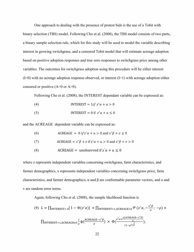
One approach to dealing with the presence of protest bids is the use of a Tobit with
binary selection (TBS) model. Following Cho et al. (2008), the TBS model consists of two parts,
a binary sample selection rule, which for this study will be used to model the variable describing
interest in growing switchgrass, and a censored Tobit model that will estimate acreage adoption
based on positive adoption responses and true zero responses to switchgrass price among other
variables. The outcomes for switchgrass adoption using this procedure will be either interest
(I=0) with no acreage adoption response observed, or interest (I=1) with acreage adoption either
censored or positive (A=0 or A>0).
Following Cho et al. (2008), the INTEREST dependant variable can be expressed as:
(4) INTEREST 1 0
(5) INTEREST 0 if 0
and the ACREAGE dependent variable can be expressed as:
(6) ACREAGE 0 0 and 0
(7) ACREAGE if 0 and 0
(8) ACREAGE unobserved if ′ 0
where z represents independent variables concerning switchgrass, farm characteristics, and
farmer demographics, x represents independent variables concerning switchgrass price, farm
characteristics, and farmer demographics, α and β are conformable parameter vectors, and u and
v are random error terms.
Again, following Cho et al. (2008), the sample likelihood function is
(9) ∏INTEREST 1 Φ ∏INTEREST ,ACREAGE , ;
∏INTEREST ,ACREAGEACREAGE Φ
ACREAGE
,

23
where Φ is the standard normal cumulative distribution function and Ψ is the bivariate standard
normal cumulative distribution function. This formula consists of three components; the first
representing the probability of a farmer being uninterested, the second representing the
probability of a farmer being interested but unwilling to convert acreage at the specific price, and
the third representing the acres that would be converted among the farmers that are interested
and are willing to accept the specified price.
To determine if a TBS model is to be used, the estimated value of ρ has to be obtained. If
the estimated value for ρ is not significantly different from zero, then a sample selection problem
is not statistically significant, and a simpler modeling procedure can be used (English 2002),
which in this case means that separate models can be used to analyze the data; a Probit on
INTEREST and a Tobit model for ACREAGE. The INTEREST dependant variable can be
expressed as:
(10) INTEREST 1if 0
(11) INTEREST 0 if 0,
and estimated using a Probit model. The likelihood function is:
(12) ∏INTEREST 1 Φ ∏ Φ .
The ACREAGE dependent variable can be expressed as:
(13) ACREAGE 0 if 0
(14) ACREAGE if 0,
and estimated using a Tobit model, which is censored at zero acres to be converted. The
likelihood function for the Tobit model is:
(15) ∏ 1 ΦACREAGE ∏ACREAGEACREAGE
.

24
Hypothesized Effects
SWITSHR is a variable that represents the share of total acres that a producer would be willing
to convert to switchgrass production. It is a discrete variable that can have a value between 0 and
1.
INTEREST is a variable representing the producer’s interest in growing switchgrass as a
crop to be used for energy production. It takes a value of if the producer is at least somewhat
interested in growing switchgrass and 0 if the producer is not. A producer’s level of interest is
hypothesized to be a product of switchgrass characteristics, switchgrass production, and how
switchgrass may affect a farming operation.
DEAGE is a variable that represents age of the producer, indexing it by dividing age by
ten. With some innovations, the period of time that it would take to see benefit from their
implementations could take several years. Intuitively, it can be concluded that a potential adopter
of an advanced age would not bother to implement a new technology or plant a new crop
because they would not see the payoff from its use. Switchgrass is a perennial crop with a stand
life of up to 10 years or more (Lewandowski et al. 2003). Therefore, farmers who do not see
their selves farming for that long would be less likely to adopt switchgrass as a crop. This
reasoning alone would lead one to think that age would have a negative effect on the adoption of
switchgrass; however, other attributes of age have to be considered. With a young farmer that is
just starting out, the drive and the willingness to try new things and take risks could be assumed
to be higher than a farmer of middle age that may be much more set in his or her ways. That
being said, the ability of the middle aged farmer to have access to the funding to start a stand of
switchgrass and also to make it through the first two years where the return would not be optimal
would in most cases be higher than that of a young farmer. It may be the case that the inability of

25
the young farmer to take the financial risk and the lack of interest of a significantly older farmer
might offset each other making the effect and magnitude of age ambiguous on both interest in
growing switchgrass and share of acres devoted to switchgrass production.
EDUCATION is a variable that indexes the level of education that the producer has
attained. It can have a value of one through six, with one representing elementary/middle school
education, two representing some high school, three representing completion of high school, four
representing some college, five representing college graduation, and six representing a post
graduate degree. Exposure to higher levels of education can increase a farmer’s management
capacity (Ellis 2006) and allow the producer to more completely understand the beneficial
options at his or her disposal. Based on these factors, Ellis (2006) hypothesized that higher levels
of attained education would have a positive effect on switchgrass adoption. However, having a
more advanced management capacity and a better understanding of the innovations available for
adoption could decrease the chance of switchgrass adoption if, in fact, the farm operation in
question is less suited to its cultivation. Because of this, it is hypothesized that EDUCATION
will have an ambiguous effect on interest in growing switchgrass and the share acres devoted to
switchgrass production.
The ownership of hay equipment and the production of hay are represented by the
dummy variables HAY1, HAY2, and HAY3. HAY1 has a value of one if the producer both own
hay equipment and produces hay. HAY2 has a value of one if the producer has hay equipment
but does not produce hay. HAY3 has a value of one if the producer does not have hay equipment
but does produce hay. Switchgrass is a crop whose harvesting utilizes the same farm implements
as hay (Jensen et al. 2007). If a farmer already produces hay, reason serves to say that they
would be more familiar with the process of harvesting grass as a profitable enterprise. Also, they

26
would already either have the equipment necessary for harvest or have a working relationship
with a custom harvest service. Jensen et al. (2007) found hay equipment to have a statistically
significant positive effect on the hectare share planted to switchgrass. Hence, it is hypothesized
that HAY1, HAY2, and HAY3 will have a positive effect on interest in growing switchgrass and
percentage of acreage devoted to switchgrass production.
CUSTHAY is a dummy variable that indicates whether or not the producer used a custom
hay harvest service in 2008. It has a value of 1 if the producer did use a custom hay harvest
service, and a value of 0 if the producer did not use a custom hay harvest service. Using a custom
hay harvest service indicates familiarity with the process of producing grass and shows that the
producers is experienced in dealing with third parties in said production. Because of this, it is
hypothesized that CUSTHAY will have a positive effect on interest in growing switchgrass and
the share of acres devoted to switchgrass production.
PRICE is a discrete variable that indexes the different dollar values producers were
offered to be willing to sell switchgrass if transportation of the biomass from the farm is
provided. The prices offered where 40, 60, 80, 100, and 120 USD. Higher prices offered should
have a positive influence on the adoption of switchgrass because it raises the incentive to
produce it, therefore price is hypothesized to have a positive effect on the share of acres to be
devoted to switchgrass production.
BEEF is a dummy variable that indexes producers’ ownership of beef cattle. The variable
has a value of one if the producer owns beef cattle and a value of zero if the producer does not.
Cattle grazing may compete with switchgrass for pasture acreage and other lands suitable to its
production. Also, with owners of beef cattle, switchgrass may have to compete with the
production of other established types of grasses that are used conventionally for hay. Therefore
27
BEEF is hypothesized to have a negative effect on the share of acres devoted to switchgrass
production.
DECACRE is a continuous variable representing the size of the producer’s farm by
indexing the total farm acreage divided by 10. There is a basic hypothesis about technology
transfer that the adoption of an innovation will tend to occur earlier on larger farms sooner than
on small farms (Fernandez-Cornejo, Daberkow, and McBride 2001). This could be due to the
uncertainty of innovation and the fixed cost associated with innovations (Fernandez-Cornejo,
Daberkow, and McBride 2001). Generally, it can be assumed that a large farm is the product of a
farmer that is more willing to take financial risk. Also, a large farm would have more access to
capital in the form of accounting profits made and loans to fund the adoption of a new crop. Ellis
(2006) found that total acres farmed had a statistically significant positive effect on switchgrass
adoption. For these reasons, it is hypothesized that farm size, Represented by DECACRE, will
have a positive effect on interest in growing switchgrass and the share of acres devoted to
switchgrass production.
RENTSHR is a variable representing the percentage of the producer’s total acreage that is
rented from another land owner. Land ownership is widely believed to encourage adoption of
innovation (Fernandez-Cornejo, Beach, and Huang 1994). In the case of switchgrass, many of
the characteristics and positive attributes of its cultivation lend it toward being planted on land
owned by the person doing the farming. These include but are not limited to its long stand life as
a perennial, prevention of erosion, and use as wildlife habitat. Jensen et al. (2007) found that the
increased percentage of leased land had a negative effect on the hectare share planted to
switchgrass. Because of this, it is hypothesized by this study that the percent of land being leased
will have a negative effect on the share of acres devoted to switchgrass production.

28
RELUCTNE is a discrete variable that indexes how a producer feels about taking
financial risks and how it affects being a successful farmer. The variable can take on values of
one through five, with one being more risk taking and five being more risk adverse. Growing
switchgrass as a dedicated energy crop is an innovative production option. Several studies (e.g.
Fernandez-Cornejo, Beach, and Huang 1994; Daberkow and Mcbride 1998; Fernandez-Cornejo,
Daberkow, and McBride 2001) have found that early adopters of innovations tend to be less risk
adverse than those that choose not to be early adopters. Therefore, it will be hypothesized by this
study that RELUCTNE will have a negative effect on interest in growing switchgrass and the
share of acres devoted to switchgrass production.
LINPUT is a variable that indexes the importance that the producer feels that
switchgrass’s possibility of having lower fertilizer and herbicide applications as compared to
other more conventional crops has on the decision to grow switchgrass. It has a value of one
representing a high level of importance and a value of zero representing a low level of
importance. Lower levels of herbicide and fertilizer associated with switchgrass could have the
positive attribute of making a lower impact on the environment through chemical pollution per
acre than more chemically intensive row crops. The lower use of herbicides and fertilizers could
represent lower input costs which might be attractive to producers. Therefore, LINPUT is
hypothesized to have a positive effect on interest in growing switchgrass.
PLANCON is a variable representing the possible conflicts between the planting and
harvesting period for switchgrass and the planting and harvesting period for other crops. It has a
value of one representing a high level of importance and a value of zero representing a low level
of importance. If a producer sees that there could be a high potential for timing conflicts between
switchgrass and other crops which may be more conventional and about the producer may be

29
more knowledgeable, there may be less inclination to plant switchgrass as an energy crop.
Because of this PLANCON is hypothesized to be negatively associated with interest in growing
switchgrass.
CONLEASE is a variable that represents the producer’s concerns about planting a
perennial crop on land that is leased. It has a value of one representing a high level of importance
and a value of zero representing a low level of importance. Switchgrass is a perennial crop with a
stand life of 10 years or more, which may cause issues with planting on land leased for less than
that period of time. If a producer places a high importance on this issue, he or she may be less
interested in growing switchgrass. Therefore, CONLEASE is hypothesized to be negatively
associated with interest in growing switchgrass.
CONCAP is a variable that represents the importance that the producer places on the
concern about having the financial and equipment resources needed to produce switchgrass. It
has a value of one representing a high level of importance and a value of zero representing a low
level of importance. Switchgrass, as with any crop, requires financial investment. If a producer
sees this issue as being highly important, he or she may show less interested in switchgrass
production. Therefore, CONCAP is hypothesized to be negatively associated with interest in
growing switchgrass.
DIVERSE is a variable that represents the importance that the producer places on the
opportunity that switchgrass may allow them to diversify his or her farming operation. It has a
value of one representing a high level of importance and a value of zero representing a low level
of importance. The opportunity to be a diversifying crop is hypothesized to be a positive attribute
of switchgrass. The more importance the producer places on diversification, the more interest
30
they may show in growing switchgrass. Because of this, it is hypothesized that DIVERSE will be
positively associated with interest in growing switchgrass.
ENERENV is a variable that represents how much importance the producer places on
switchgrass’s possible ability to contribute to national energy and help the environment by
producing switchgrass for fuel. These are hypothesized to be positive aspects of switchgrass
production. Therefore, it is hypothesized that ENERENV will be positively associated with
interest in growing switchgrass.
LAGPOT is a variable that represents the importance that the producer places on the
three year lag between planting and switchgrass reaching its full yield potential. It has a value of
one representing a high level of importance and a value of zero representing a low level of
importance. The lag time between planting switchgrass and realizing the full potential of a
switchgrass stand is one of the perceived drawbacks to planting switchgrass as an energy crop. If
the producer sees this as important issue, he or she may be less interested in producing
switchgrass for energy production. Because of this, it is hypothesized that LAGPOT will be
negatively associated with interest in growing switchgrass.
COMPKNOW is a variable that represents the importance that the producer places on the
comparison between his or her knowledge of switchgrass compared to other crops. Because
switchgrass is a new crop, information regarding its production may not be as widely
disseminated as other more conventional crop options. If a producer puts a high level of
importance on the discrepancy between his or her knowledge of switchgrass compared to other
crops, they may be less likely to be interested in growing switchgrass. Because of this, it is
hypothesized that COMPKNOW will have a negative effect on interest in growing switchgrass.

31
SWEST, MIDS, and GULF are dummy variables that represent states in the southwest
(OK, TX), mid-south (TN, KY, AR), and gulf regions respectively (LA, MS, AL). The omitted
regional dummy represents the Atlantic states in the study region (GA, NC, SC, VA).
CRP and CRPACSHR are variables that describe the producer’s Conservation Reserve
Program situation. CRP is a dummy variable with a value of 1 if the producer currently has acres
enrolled and a value of 0 if the producer does not. CRPACSHR is a variable that represents the
percentage of farm acres that the producer has in the CRP program. It may be the case that a
producer with land in the CRP program is more concerned about environmental preservation
than one who does not. One perceived benefit of switchgrass is that it may be less harmful on the
environment that traditional row crops, which could appeal to an environmentally conscious
producer. Hence, CRP is hypothesized to have a positive effect on interest in switchgrass.
Because of the length of CRP contracts, land that is currently in CRP may be locked as such for
several years in the future. The higher the percentage of land in CRP, the less percentage of land
there is free to be converted to other uses, such as planting switchgrass. Because of this,
CRPACSHR is hypothesized to have a negative effect on the acre share of switchgrass
converted.
IDLED and IDLESHR are variables that deal with acres of land a producer has that have
been left idled. IDLED is a dummy variable that has a value of 1 if the producer has any farm
acres that have been left idled and a value of 0 if the producer does not. Land that has been left
idled may have been utilized in that way because factors such as available soil nutrients, water
availability, or erosion issues have prevented it from being used for conventional farming
activities. Because switchgrass is a potential crop that has the ability to grow on marginal lands
(Lewandowski et al. 2003) with the ability to help prevent erosion (Ellis 2006), any acreage that

32
is idled due to poor yield or erosion problems with conventional crops could be productive under
the cultivation of switchgrass. Therefore, IDLED is hypothesized to have a positive effect on
producer interest in switchgrass and IDLESHR is expected to have a positive effect on the share
of acres planted to switchgrass.
COMCON is a dummy variable that indicates if the producer has ever produced a
commodity under contract. It has a value of 1 if the producer has produced a commodity under
contract and a value of 0 if the producer has not. Contracts can be a way of reducing risk
associated with uncertainty in prices and demand of a commodity. It is hypothesized that
switchgrass may be sold primarily under contract and farmers who have experience dealing with
contract sales may be more interested in growing switchgrass. However, it is possible that the
producer has grown a commodity under contract and did not have a positive experience. This
could lead to them being leery of doing so again. Because of this, it is hypothesized that
COMCON will have a negative effect on the share of acres planted.
NOEROS is a dummy variable indicating whether or not the producer has significant
erosion problems on his or she land. It has a value of 1 if the producer has significant erosion
problems and 0 if the producer does not. One of the positive attributes of switchgrass production
is that it has the potential to reduce erosion. If the farmer does not have erosion problems, he or
she may be less likely to show interest in growing switchgrass. Therefore, it expected to have a
positive influence on interest in growing switchgrass.
Off-farm income of the decision maker is a factor that has been analyzed by several adoption
studies. Norris and Batie (1987) found off-farm income to have a negative effect on conservation
practice expenditures and Fernandez-Cornejo, Hendricks, and Mishra (2005) found it to have a
positive effect on adoption of integrated pest management practices. For this study, off-farm

33
income will be analyzed using the variables OFIL10, OFI1030, and OFI3050. OFLI10 represents
producers with less than 10,000 dollars in off-farm income in 2008, OFI1030 represents farmers
with greater than 10,000 dollars but less than 30,000 dollars in off-farm income in 2008, and
OFI3050 represents farmers with greater than 30,000 dollars but less than 50,000 dollars in off-
farm income. Having a higher off-farm income could mean that the producer would have access
to more capital to establish a switchgrass stand. Also, having a higher off-farm income could
mean that the producer may be able to rely less on farm income and might therefore be willing to
take more risk with his or her farming operation. for these reasons, OFIL10, OFI1030, and
OFI3050 are hypothesized to have a positive effect on interest in growing switchgrass and the
share of acres that the producer is willing to convert to switchgrass.
Data
“Switchgrass Production for Energy: Your Views” is the title of a mail survey conducted to
collect data for use in estimating farmers’ willingness to convert acreage to switchgrass. This
survey will be the basis for the data analyzed in this study. For the survey, farmers with farms
having at least $10,000 in sales were randomly selected by the National Agricultural Statistics
Service from the following states: Alabama, Arkansas, Georgia, Kentucky, Louisiana,
Mississippi, North Carolina, Oklahoma, South Carolina, Tennessee, Texas, and Virginia.
The mail survey consisted of 39 questions and was sent out to 7,000 farmers. The
questions were designed and selected to evaluate the influences of demographics, farm
characteristics, and attitudes toward environmental issues. The five major areas addressed in the
survey were 1) the respondent’s knowledge of, and interest in, switchgrass as an energy crop; 2)
the respondent’s opinion on a number of topics related to switchgrass production as a biomass
feedstock; 3) characteristics of the farm operation, including types of enterprises and use of

34
various agricultural practices; 4) financial matters, including sources and extent of income; and
5) socio-demographic characteristics of the respondents.
The initial mailing of the survey included a cover letter explaining its purpose and a
postage-paid return envelope. There was a follow-up reminder postcard sent a week after the
initial mailing. A follow-up mailing that included a letter emphasizing the importance of the
survey, and another copy of the questionnaire was sent two weeks after the mailing of the
reminder postcard. A total of 1,322 surveys were returned and recorded for an 18.9 percent
response rate. Copies of the survey instrument and cover letter are provided in the Appendix.
Results
A total of 760 observations remained after rejecting observations with missing values for
the variables used in the model. Of these remaining responses, 67.34% of the producers claimed
to be at least somewhat interested in growing switchgrass as an energy crop. This percentage of
interested respondents compares favorably with Jensen et al. (2007) which found that 29.6% of
Tennessee respondents would be interested and Wen et al. (2009) which found that 43% of
southern Virginian respondents would definitely be interested in growing switchgrass. Of these
responses that showed interest in growing switchgrass (N=512), the average number of acres
they would be willing to convert to switchgrass was 76.67, which equal to a 24.46% share of
acres farmed for these respondents. This is a higher number in comparison to the findings of
Wen et al. (2009) and Jensen et al. (2007), which were 66 average acres and 67.21 average acres
converted per farm respectively.
35
Tobit Model with Sample Selection
As previously discussed, the dependant variables INTEREST and SWITSHR were
estimated as a Tobit model with sample selection. The estimated coefficient for ρ (.0802) was
statistically significant at α=.10, meaning that the model was significant overall compared to
running separate Tobit and Probit models with the variables. A chi-squared test was also used to
test the significance of the Tobit Model with Sample Selection compared to separate Tobit and
Probit models. The log likelihood ratio (LLR) for the test was found using the following formula:
(16) 2 .
Using this formula, the LLR was computed to be 3.325. The chi-squared statistic for the .10 level
of significance and one degree of freedom is 2.71, with the rejection region being to the right of
this value. The LLR for this test falls in the rejection region, therefore the hypothesis that the two
equations should be estimated separately should be rejected.
Probit Selection Equation for INTEREST
Farm and Farmer Variables
The coefficient for DECAGE is negative and statistically significant which suggest that
older producers would be less likely to be interested in producing switchgrass. This corresponds
with the findings of Daberkow and McBride (1998) and Norris and Batie (1987). Producers with
beef cattle operations are less likely to be interested, as suggested by BEEF having a negative
coefficient. Reluctance to adopt new production methods or crops before one sees them work for
someone else appears to be a trait that lowers the likelihood of a producer being interested as
evidenced by the variable RELUCTNE having a negative and significant coefficient. This
corresponds to several other studies (e.g. Fernandez-Cornejo, Beach, and Huang 1994;
Daberkow and Mcbride 1998; Fernandez-Cornejo, Daberkow, and McBride 2001) that found

36
that early adopters of innovations tend to be less risk adverse than those that choose not to be
early adopters. The estimated coefficient for the dummy variable MIDS was negative and
significant, indicating that producers in the mid-south region are less likely to be interested in
growing switchgrass than producers in the unobserved Atlantic region.
The coefficients for HAY1 and HAY2 were positive and significant suggesting that
owning hay equipment and the combination of owning hay equipment and producing hay on
one’s farm make producers more likely to be interested. This corresponds with what Jensen et al.
(2007) found with hay equipment having a statistically significant positive effect on the hectare
share planted to switchgrass Likewise, the use of custom hay harvest services influences
producers to be more likely to be interested. Not having significant erosion problems appears to
lower a farmer’s likelihood of being interested, as NOEROS has a negative and significant
coefficient. The estimated coefficients for HACFARM, EDUCATIO, SWEST, GULF, IDLED,
CRP, OFI1030, and OFI3050 were not significantly different than zero.
Opinion Variables
As expected PLANCON, CONLEASE, and CONCAP all had coefficients that were
significant and negative, suggesting that these factors negatively impact a producer’s likelihood
of being interested. LINPUT, DIVERSE, and ENERENV also had expected results with
coefficients that were significant and positive, suggesting that these factors negatively impact a
producer’s likelihood of being interested. The dummy variable representing the lowest level of
off-farm incomes, OFIL10, is negative and significant, indicating that producers with off-farm
incomes less than 10,000 dollars are less likely to be interested in growing switchgrass than a
producer with the omitted off-farm income of 50,000 dollars or more. This corresponds with the
findings of Fernandez-Cornejo, Handricks, and Mishra (2005) that producers with a higher off-
37
farm income are more likely to be early adopters of innovation. The estimated coefficients for
COMCON, LAGPOT, and COMPKNOW were not significantly different than zero.
Tobit Regression for the Share of Acres Producers are Willing to Convert to Switchgrass
The estimated coefficient for PRICE is positive and significant, showing that producers
in the study may be price responsive. Contrary to what was hypothesized, the estimated
coefficient for HACFARM is negative and significant, indicating that larger farms are willing to
devote a lower percentage of acreage to the production of switchgrass than smaller farms. The
estimated coefficient for DECAGE is positive and significant, indicating that older producers are
willing to devote a lower percentage of acreage to the production of switchgrass than smaller
farms. The estimated coefficient for SWEST and GULF is positive and significant, indicating
that producers in these regions are willing to devote a higher percentage of acreage to the
production of switchgrass than producers in the Atlantic region. The reluctance to adopt new
production methods or crops before one sees them work for someone else appears to have a
negative effect on the share of acres a producer is willing to switchgrass, as evidenced by the
coefficient for RELUCTNE being negative and significant.
The estimated coefficient for COMCON is negative and significant, indicating that
producers that have previously produced commodities under contract are likely to devote a
smaller percentage of acreage to the production of switchgrass than producers that have not
produced commodities under switchgrass. The coefficient for HAY3 is negative and significant,
which is contrary to what was hypothesized, indicating that producing hay while not currently
own hay harvesting equipment has a negative effect on the share of acres a producer is willing to
devote to switchgrass. The estimated coefficient for CRPACSHR is negative and significant,

38
indicating that farms with larger acre shares of CRP land are likely to devote a lower percentage
of acreage to the production of switchgrass.
Conclusions
The results of this study have several possible implications for switchgrass production
and adoption expansion efforts in the southeastern United States. Based on the results,
individuals and organizations that want to promote interest in adopting switchgrass may want to
emphasize switchgrass’ positive attributes, such as its potential for lowering input requirements,
its ability to diversify a producer’s crop mix, and the possibility of it contributing to the nation’s
energy security and environment. Also, farmers that have erosion problems on their land showed
higher interest in switchgrass production, which means that switchgrass’ ability to reduce erosion
compared to more traditional crops could be emphasized as well. Concerns that affect
producers’ interest in growing switchgrass that likely need to be addressed through educational
programs include management techniques to deal with possible conflicts between the planting
and harvesting of switchgrass and other crops, contract arrangements that enable planting of
switchgrass on land that is leased, and efficient use of financial and equipment resources needed
to produce switchgrass.
From the results, it can be concluded that older producers would be less interested in
switchgrass production, as they may not continue farming long enough to see the full benefits of
a switchgrass stand. Those producers that operate a beef cattle operation are likely to be less
interested, as well. This may be due to the reluctance of these producers to convert acres of
pasture to switchgrass production and seems to indicate that areas with a high percentage of beef
cattle farmers may not be an ideal switchgrass production area. Contrarily, producers that own
hay equipment or have used custom hay harvest service may be more likely to be interested in

39
growing switchgrass. Hence, switchgrass may be first adopted by producers who already have
equipment that may be helpful in growing switchgrass.
The results of this study indicate that the share of acres that would be converted to
switchgrass will be less on a larger farm. Also, while older farmers may be less willing to adopt
switchgrass, those that do may be willing to devote more acreage that a younger farmer. This
indicates that areas with smaller farms and younger farmers, on average, may show more acres
being converted to switchgrass, ceteris paribus. Those producers who are reluctant to adopt a
new crop before they see it work for others reasonably may show less interest in producing
switchgrass and if they are willing to adopt, will likely convert a smaller share of acreage to
switchgrass. Producers with a higher percentage of acreage devoted to CRP land may show a
likelihood of devoting a smaller share of acres to switchgrass, which indicates that areas with
producers that have a higher portion of their land devoted to CRP may devote a smaller portion
of acres to switchgrass. This result suggests that CRP rules may need to be modified to
encourage switchgrass production in a sustainable way on CRP lands. The results show that
producers are sensitive to price with respect to both adopting switchgrass and the share of acres
they would be willing to convert, indicating that a higher price offered at the plant gate should
mean that a bio-refinery will receive more biomass.
This study has given new information about switchgrass production from the producer’s
prospective in the southeastern U. S. However, there is still a substantial lack of knowledge in
related areas, such as contract preferences or harvesting and storage arrangements, that future
studies can build upon.

40

41
References
Abadi Ghadim, A.K. and D.J. Pannell . 1999. “A Conceptual Framework of Adoption of an
Agricultural Innovation.”Agricultural Economics21(2):145-154.
Adesina, A.A. 1996. “Factors Affecting the Adoption of Fertilizers by Rice Farmers in Côte
d’Ivoire.” Nutrient Cycling Agroecosystems46:29-39.
Baidu-Forson, J. 1999. “Factors Influencing Adoption of Land-Enhancing Technology in the
Sahel: Lessons from a Case Study in Niger.” Agricultural Economics 20:231-239.
Bocqueho, G., and F. Jacquet. 2010. "The Adoption of Switchgrass and Miscanthus by Farmer:
Impact of Liquidity Constraints and Risk Preferences." Energy Policy 38(5): 2598-2607.
Bransby, D. I.1998. “Interest Among Alabama Farmers in Growing Switchgrass for
Energy.”Paper presented at BioEnergy '98: Expanding Bioenergy Partnerships,
MadisonWI, Oct. 4-8.
Bransby, D. I. 2005. "Switchgrass Profile". Bioenergy Feedstock Information Network
(BFIN),Oak Ridge National Laboratory.
Cho, S., S. Yen, J. Bowker, and D. Newman. 2008. “Modeling Willingness to Pay for Land
Conservation Easements: Treatment of Zero and Protest Bids and Application and Policy
Implications.” Journal of Agricultural and Applied Economics 40(1):267-285.
Daberkow, S. and W. McBride. 1998. “Socio-economic Profiles of Early Adopters of Precision
Agricultural Technologies.” Journal of Agribusiness 16(2):151-168.
Ellis, P. C. 2006 “Factors that Influence the Decision to Adopt Switchgrass for Energy
Production.” MS thesis, University of Tennessee, Knoxville.
Feder, G., R. E. Just, and D. Zilberman. 1985. “Adoption of Agricultural Innovations in
Developing Countries: A Survey.” Economic Development and Cultural Change
33(2):255-98.

42
Fernandez-Cornejo, J., D. Beach, and W. Huang. 1994. "The Adoption of IPM Techniques by
Vegetable Growers in Florida, Michigan and Texas," Journal of Agricultural andApplied
Economics 26(1): 158-172.
Fernandez-Cornejo, J., S. Daberkow, and W. D. McBride. 2001. “Decomposing the Size Effect
on the Adoption of Innovations: Agro-biotechnology and Precision Farming.” Paper
presented at the American Agricultural Economics Association Annual Meeting, Chicago,
IL. Aug. 5-8.
Fernandez-Cornejo, J., C. Hendricks, and A. Mishra. 2005. Technology Adoption and Off-farm
Income: The Case of Herbicide-Tolerant Soybeans. Journal of Agricultural and Applied
Economics 37(3): 549-563.
Hahn-Hagerdal B., M. Galbe, M. Gorwa-Grauslund, G. Liden, and G. Zacchi. 2006. Bio-ethanol:
the Fuel of Tomorrow from the Residues of Today.” Trends in Biotechnology 24:549-
556.
Hipple, P.C., and M.D. Duffy. 2002. “Farmer’s Motivation for Adoption of Switchgrass.” Trends
in New Crops and New Uses p.252-266.
Janick, J., M.G. Blase, D.L. Johnson, G.D. Joliffe, and R.L. Myers. 1996. Diversifying U.S. crop
production. P. 98-108. In: J. Janick (ed.), Progress in new crops. ASHS Press,
Alexandria, VA.
Jensen, K., C. D. Clark, P. Ellis, B. English, J. Menard,M. Walsh, and D. L. T. Ugarte. 2007.
“Farmer Willingness to Grow Switchgrass for Energy Production.” Biomass & Bioenergy
31:773-781.
Kaltschmitt, M. 1996. “The Benefits and Costs of Energy from Biomass in Germany”Biomass &
Bioenergy 6(5):329-337.

43
Kelsey, K. and T. Franke. 2009. “The Producers’ Stake in the Bioeconomy: A Survey of
Oklahoma Producers’ Knowledge and Willingness to Grow Dedicated Biofuel Crops.”
Journal of Extension 47(1):1-6.
Larson, J., B. English, and L. He. 2005. “Risk and Return for Bioenergy Crops under Alternative
Contracting Arrangements.” Paper presented at the Southern AgriculturalEconomics
Association Annual Meetings, Dallas TX, February 2-6.
Larson, J., B. English, C. Hellwinckel, D. Ugarte. 2005. “A Farmer Evaluation of Conditions
under Which Farmers Will Supply Biomass Feedstocks for Energy Production.” Paper
presented at the American Agricultural Economics Association Annual Meeting,
Providence RI, July 24-27.
Lewandski, I., J. M. O. Scurlock, E. Lindvall, and M. Chirstou. 2003. “The Development of
Perennial Rhizomatous Grasses as Energy Crops in the U. S. and Europe.” Biomass &
Bioenergy 25(4):335-361.
Lindner, R.K. 1987. “Adoption and Diffusion of Technology: an Overview.” In: Champ, B.R.,
E.Highly, J.V. Remenyi. “Technological Change in Postharvest Handling and
Transportation of Grains in the Humid Tropics.” ACIAR Proceedings Series, Australian
Centre for International Agricultural Research, 19:144-151.
Ma, Z., C. Wood, and D. Bransby. 2000. “Carbon Dynamics Subsequent to Switchgrass
Establishment.” Biomass and Bioenergy 18:93-104.
Marra, M., D. Pannell, and A. Ghadim. 2003. “The Economics of Risk, Uncertainty andLearning
in the Adoption of New Agricultural Technologies: Where are We on theLearning
Curve?” Agricultural Systems 75:215-234.

44
McLaughlin, S. B., and L. A. Kszos. 2005. “Development of Switchgrass (Panicum virgatum) as
a Bioenergy Feedstock in the United States.” Biomass & Bioenergy 28(6):515-535.
Mitchell, R., K. Vogel, and G. Sarath. 2008. “Managing and Enhancing Switchgrass as a Bio-
energy Feedstock.” Biofuels, Bioproducts, and Biorefining 2:530-539.
Nkonya E., T. Schroeder, and D. Norman. 1997. “Factors Affecting Adoption of Improved
Maize Seed and Fertilizer in Northern Tanzania.” Journal of Agricultural Economics
48:1-12.
Norris, P. E., and S. S. Batie. 1987. “Virgina Farmers’ Soil Conservation Decisions: an
Application of Tobit Analysis.” Southern Journal of Agricultural Economics 19:79-90.
Paulrud, S., and T. Laitila. 2010. “Farmers’ Attitudes about Growing Energy Crops: A Choice
Experiment Approach” Biomass and Bioenergy 34(12):1770-1779.
Perlack, R. D., L. L. Wright, A. F. Turhollow, L. R. Graham , B. J. Stokes, and D. C. Erbach.
2005. “Biomass as Feedstock for a Bioenergy and Bioproducts Industry: the Technical
Feasibility of a Billion-Ton Annual Supply.” U.S. Department of Agriculture and U. S.
Department of Energy, Oak Ridge TN, April.
Rajasekharan, P., and S. Veeraputhran. 2002. “Adoption of Intercropping in Rubber
Smallholdings in Kerala, India: a Tobit Analysis.” Agroforestry Systems 56:1-11.
Ransom J. K., K. Paudyal, and K. Adhikari. 2003. “Adoption of Improved Maize Varieties in the
Hills of Nepal.” Agricultural Economics23:299–305.
Sissine F. 2007. “Energy Independence and Security Act of 2007: A Summary of Major
Provisions” Congressional Research Service CRS report no. RL34294.
Stubbendieck, J., S. L. Hatch, and C. H. Butterfield. 1992. “North American Range Plants.”
Fourth edition. University ofNebraska Press, Lincoln, Nebraska, USA.

45
Velandia, M., D. Lambert, J. Fox, J. Walton, and E. Sanford. 2010. “Intent to Continue Growing
Switchgrass as a Dedicated Energy Crop: A Survey of Switchgrass Producers in East
Tennessee.” European Journal of Social Sciences 15(35):299-312.
Walton, J., J. Larson, R. Roberts, D. Lambert, B. English, S. Larkin, M. Marra, S. Martin, K.
Paton, and J. Reeves. 2010. “Factors Influencing Farmer Adoption of Portable Computers
for Site-specific Management: A Case for Cotton Production.” Journal of Agricultural &
Applied Economics 42(2): Forthcoming.
Wang, M. 2008. “Well-to-Wheels Energy and Greenhouse Gas Emission Results and Issues of
Fuel Ethanol.” Farm Foundation Agriculture and the Environment: Lifecycle Carbon
Footprint of Biofuels Workshop, January 29, 2008, Miami Beach, Florida.
Wen, Z., J. Ignosh, D. Parrish, J. Stowe, and B. Jones. 2005. “Identifying Farmers’ Interest in
Growing Switchgrass for Bio-energy in Southern Virginia.” Journal of Extension
47(4):5RIB7.

46
Appendix A: Tables

47
Table A.1. Farm and farmer demographics for the sample. Characteristics Census Averages Survey Respondent Percentages Net Farm Income Before Taxes Negative (Less than $0) $0 - $9,999 $10,000 - $14,999 $15,000 - $19,999 $20,000 - $24,999 $25,000 - $29,999 $30,000 - $34,999 $35,000 - $39,999 $40,000 - $44,999 $45,000 - $49,999 $50,000 - $74,999 $75,000 - $99,999 $100,000 - $149,999 At least $150,000 Net Off-farm Income Before Taxes Negative (Less than $0) $0 - $9,999 $10,000 - $14,999 $15,000 - $19,999 $20,000 - $24,999 $25,000 - $29,999 $30,000 - $34,999 $35,000 - $39,999 $40,000 - $44,999 $45,000 - $49,999 $50,000 - $74,999 $75,000 - $99,999 $100,000 - $149,999 At least $150,000 Education Level Obtained: Elementary/Middle school Some high school High school Some college College graduate Post graduate
68.63% (< 9,999)
12.65%(10,000- 24,999)
6.18%(25,000- 49,999)
3.55%(50,000- 99,999) 8.98%(> 100,000)
- - - - - - - - - - - - - -
- - - - - -
16.02% 28.63% 12.61% 6.48% 5.43% 4.90% 3.50% 2.28% 2.01% 1.58% 4.47% 2.89% 3.77% 5.43%
(N=1142)
5.8% 7.52% 4.71% 2.90% 3.53% 4.98% 4.80% 4.71% 5.34% 6.25% 17.3%
11.87% 9.60%
10.69% (N=1104)
1.91% 3.03%
29.19% 24.32% 26.63% 14.91%
(N=1254)

48
Table A.2. Farm and farmer demographics for the sample cont. Characteristics Census Average Survey Respondent Percentages Total Acres: Acres owned Acres rented Acres rented to others Total acres farmed Age of Operator Farming Experience
318.82 acres - - -
58.0
-
Mean 240.59 acres 131.62 acres 194.68 acres 384.21 acres
60.28 years
35.3 years

49
Table A.3. Familiarity and interest in growing switchgrass as an energy crop. Familiarity with switchgrass as a crop to be used in
energy production (Percent) Interest in Growing Switchgrass as an Energy Crop
Not at all familiar (N=631)
Somewhat familiar (N=434)
Very familiar (N=33)
Not at all interested (N=437) Somewhat interested (N=479) Very interested (N=182)
50.7 38.4 10.9
25.1 52.0 22.8
24.2 33.3 42.4

50
Table A.4. Farmer characteristics. Characteristic
All Survey Respondents
Not at all Interested Respondents
Somewhat Interested Respondents
Very Interested Respondents
Percent Owns a personal computer Extension workshops attended in 2008 Age Farming Experience Produced commodity under contract before Currently belongs to the following organizations : Grower/ commodity Cooperative Farm Bureau Hunting-related Environmental
74.22 (N=1253)
1.1 (avg. events)
(N=1195)
85 (N=1284)
60.3 (avg. years) (N=1241)
21.8
(N=1222)
13.9 (N=1169)
31.8
(N=1170) 57.7
(N=1172) 21.6
(N=1169) 8.7
(N=1169)
63.1 (N=471)
0.91(avg. events)
(N=485)
82 (N=468)
63.8 (avg. years) (N=504)
13.7
(N=497)
11 (N=483)
30.8
(N=483) 56.8
(N=484) 17.8
(N=483) 5.4
(N=483)
80.2 (N=531)
1.2 (avg. events)
(N=545)
87.2 (N=530)
58.6 (avg. years) (N=529)
25
(N=519)
13.2 (N=491)
32.3
(N=492) 57.4
(N=493 23
(N=491) 9.8
(N=491)
85.23 (N=210)
1.29 (avg. events)
(N=203)
87.5 (N=208)
56.3 ( avg. years) (N=208)
33
(N=206)
22.5 (N=195)
33.3
(N=195) 60.5
(N=197) 27.7
(N=195) 14.4
(N=195)

51
Table A.5. Hay equipment demographics. All Survey
Respondents Not at all interested Respondents
Somewhat interested respondents
Very Interested Respondents
Percent Owns Hay Equipment Used Custom Hay Services
61.5 (N=1235) 21.6 (N=1210)
55.1 (N=501) 20.6 (N=495)
65.7 (N=525) 21.6 (N=515)
66.5 (N=209) 24 (N=200)

52
TableA.6. Farmer concerns about risk and loss.
All Survey Respondents
Not at all interested Respondents
Somewhat interested respondents
Very Interested Respondents
Average responses from one to five with one being strongly disagree and 5 being strongly agree You are the type of farmer who is more willing to take financial risks than others You must be willing to take substantial financial risk to be a successful farmer You are reluctant about adopting new production methods or crops until you see them working for others You are more concerned about a large loss to your farming operation than about missing a substantial gain
2.7 (N=1176) 3.1 (N=1178) 3.1 (N=1184) 3.4 (N=1177)
2.5 (N=457) 3.0 (N=459) 3.4 (N=464) 3.42 (N=459)
2.7 (N=513) 3.1 (N=512) 3.1 (N=517) 3.5 (N=515)
3.2 (N=206) 3.3 (N=207) 2.5 (N=203) 3.2 (N=203)

53
Table A.7. Farm organization.
All Survey Respondents
Not at all interested Respondents
Somewhat interested respondents
Very Interested Respondents
Percent Description of farm operation Children or Grandchildren will inherit farm Land sold for development after farmer ceases Land will be sold or leased to other farmer after farmer ceases farming Other plans Livestock present on farm Farm Decisions Farm alone makes decisions Shared decision with partners or family Someone else makes the decisions Which best describes farm business Sole Proprietorship Partnership Cooperative Corporation Other
58.54 (N=1182) 7.9 (N=1182) 20.7 (N=1182)
12.9 (N=1182) 80 (N=1208) 70.7 (N=1244) 26.2 (N=1244) 3.1 (N=1244) 76.6 (N=1228) 15.2 (N=1228) .16 (N=1228) 4.2 (N=1228) 3.7 (N=1228)
52.4 (N=479) 9.2 (N=479) 23.8 (N=479) 14.6 (N=479) 78.8 (N=505) 72.5 (N=498) 22.69 (N=498) 4.6 (N=498) 78.2 (N=491) 12.8 (N=491) .41 (N=491) 3.5 (N=491) 5.1 (N=491)
60 (N=503) 7.8 (N=503) 20.5 (N=503) 11.7 (N=503) 80.7 (N=498) 70.3 (N=536) 27.6 (N=536) 2.0 (N=536) 76.2 (N=530) 16.6 (N=530) .19 (N=530) 2.1 (N=530) 2.6 (N=530)
69.5 (N=200) 5 (N=200) 14 (N=200) 11.5 (N=200) 75 (N=205) 67.1 (N=210) 40 (N=210) (N=210) 73.9 (N=207) 17.4 (N=207) 0 (N=207) 5.3 (N=207) 3.4 (N=207)

54
Table A.8. Variable means and estimated values
Variable Mean value
(N=760) Mean value
(N=512) Estimated
sign HACFARM 3.85 4.01 + EDUCATIO 4.18 4.23 ? DECAGE 5.86 5.69 ? CUSTHAY 0.22 0.23 + BEEF 0.70 0.66 - COMCON 0.24 0.29 ? HAY1 0.51 0.52 + HAY2 0.16 0.17 + HAY3 0.10 0.10 + RELUCTNE 3.06 2.91 - GULF 0.23 0.22 ? MIDS 0.32 0.30 ? SWEST 0.14 0.13 ? OFIL10 0.11 0.09 - OFI1030 0.15 0.15 - OFI3050 0.22 0.21 - PLANCON 2.44 - CONLEASE 2.17 - LINPUT 3.53 - CONCAP 3.30 - DIVERSE 3.00 + ENERENV 3.25 + LAGPOT 3.37 - COMPKNOW 2.96 - NOEROS 0.54 - IDLED 0.13 + CRP 0.15 + PRICE 82.7 + IDLESHR 0.03 + CRPACSHR 0.08 - RENTSHR 0.22 -

55
Table A.9. Estimated Tobit Model with Sample Selection
INTEREST (N1=760) SWITSHR (N2=512)
Variable Est. Coeff. Std. Err. Mean Est. Coeff. Std. Err.
Mean
Hyp. Sign
INTERCEPT 0.078 0.626 0.125 0.177
HACFARM -0.001 0.001 3.85 -0.048 0.012 *** 4.01 +
EDUCATIO -0.002 0.064 4.18 -0.006 0.018 4.23 ?
DECAGE -0.142 0.061 ** 5.86 0.036 0.019 * 5.69 ?
CUSTHAY 0.518 0.200 *** 0.22 0.044 0.048 0.23 +
BEEF -0.704 0.176 *** 0.70 -0.008 0.041 0.66 -
COMCON 0.192 0.181 0.24 -0.096 0.046 ** 0.29 ?
HAY1 0.573 0.184 *** 0.51 -0.036 0.052 0.52 +
HAY2 0.540 0.230 ** 0.16 0.118 0.060 ** 0.17 +
HAY3 0.199 0.284 0.10 -0.103 0.071 0.10 +
RELUCTNE -0.112 0.064 * 3.06 -0.055 0.018 *** 2.91 -
GULF -0.220 0.190 0.23 0.141 0.052 *** 0.22 ?
MIDS -0.321 0.180 * 0.32 0.057 0.051 0.30 ?
SWEST -0.273 0.238 0.14 0.118 0.063 * 0.13 ?
OFIL10 -0.468 0.223 ** 0.11 -0.069 0.075 0.09 -
OFI1030 -0.094 0.211 0.15 -0.081 0.054 0.15 -
OFI3050 -0.106 0.170 0.22 -0.070 0.051 0.21 -
PLANCON -0.130 0.060 ** 2.44 -
CONLEASE -0.206 0.053 *** 2.17 -
LINPUT 0.291 0.068 *** 3.53 -
CONCAP -0.146 0.066 ** 3.30 -
DIVERSE 0.442 0.075 *** 3.00 +
ENERENV 0.314 0.067 *** 3.25 +
LAGPOT 0.043 0.069 3.37 - COMPKNOW -0.052 0.057
2.96 -
NOEROS -0.251 0.141 * 0.54 -
IDLED 0.298 0.260 0.13 +
CRP -0.071 0.205 0.15 +
PRICE 0.001 0.001 ** 82.7 +
IDLESHR 0.023 0.145 0.03 +
CRPACSHR -0.109 0.038 *** 0.08 -
RENTSHR 0.019 0.058 0.22 -
σ 0.382 0.018 ***
ρ -0.265 0.152 *
The symbol ‘***’ denotes significance at =.01, ‘**’ denotes significance at =.05, and ‘*’ denotes significance at =.10.

56
Appendix B: Survey
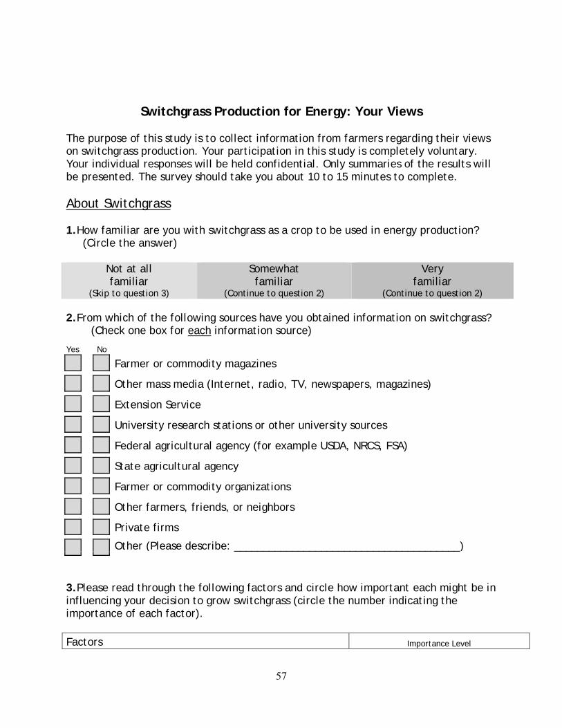
57
Switchgrass Production for Energy: Your Views
The purpose of this study is to collect information from farmers regarding their views on switchgrass production. Your participation in this study is completely voluntary. Your individual responses will be held confidential. Only summaries of the results will be presented. The survey should take you about 10 to 15 minutes to complete.
About Switchgrass
1.How familiar are you with switchgrass as a crop to be used in energy production? (Circle the answer)
Not at all familiar
(Skip to question 3)
Somewhat familiar
(Continue to question 2)
Very familiar
(Continue to question 2) 2.From which of the following sources have you obtained information on switchgrass?
(Check one box for each information source)
3.Please read through the following factors and circle how important each might be in influencing your decision to grow switchgrass (circle the number indicating the importance of each factor).
Factors Importance Level
Yes No
Farmer or commodity magazines Other mass media (Internet, radio, TV, newspapers, magazines) Extension Service University research stations or other university sources Federal agricultural agency (for example USDA, NRCS, FSA) State agricultural agency Farmer or commodity organizations Other farmers, friends, or neighbors Private firms Other (Please describe: _______________________________________)

58
Not at All Not Very
Some-what Very
Extre-mely
Possible conflicts between planting/harvest period for switchgrass and planting/harvest period for your other crops 1 2 3 4 5
Concern that the market for switchgrass as an energy crop is not developed enough yet 1 2 3 4 5
Profitability of growing switchgrass compared with other farming alternatives 1 2 3 4 5
Possibility that you will cease farming in the next few years due to retirement or other reasons 1 2 3 4 5
Your knowledge about growing switchgrass compared with your knowledge about growing other crops 1 2 3 4 5
Concern about planting a perennial crop such as switchgrass on land that is leased 1 2 3 4 5
Opportunity to diversify your farming operation 1 2 3 4 5
Potential for creating jobs in your community 1 2 3 4 5
Potential for switchgrass to reduce erosion on your farm 1 2 3 4 5
Whether acreage converted to switchgrass would qualify for CRP payments or not 1 2 3 4 5
Potential for switchgrass to provide habitat for native wildlife on your farm 1 2 3 4 5
Potential to contribute to national energy security by producing switchgrass for fuel 1 2 3 4 5
Potential to help the environment by producing switchgrass for fuel 1 2 3 4 5
Ability to use switchgrass as a feed for livestock 1 2 3 4 5
The three year lag between planting and switchgrass reaching its full yield potential 1 2 3 4 5
Possibility of lowering fertilizer and herbicide applications as compared with crops currently growing 1 2 3 4 5
Concern about having the financial and equipment resources needed to produce switchgrass 1 2 3 4 5
Other (Please describe: _________________________________________________________________ _____________________________________________________________________________________)
4. How interested are you in growing switchgrass as a crop to be used for energy production? (Circle the answer)
Not at all interested
Somewhat interested
Very interested
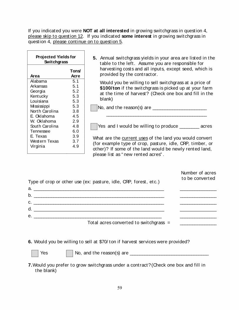
59
If you indicated you were NOT at all interested in growing switchgrass in question 4, please skip to question 12. If you indicated some interest in growing switchgrass in question 4, please continue on to question 5.
6. Would you be willing to sell at $70/ton if harvest services were provided?
Yes No, and the reason(s) are ________________________________
7.Would you prefer to grow switchgrass under a contract? (Check one box and fill in the blank)
Projected Yields for Switchgrass
Area Tons/ Acre
Alabama 5.1 Arkansas 5.1 Georgia 5.2 Kentucky 5.3 Louisiana 5.3 Mississippi 5.3 North Carolina 3.8 E. Oklahoma 4.5 W. Oklahoma 2.9 South Carolina 4.8 Tennessee 6.0 E. Texas 3.9 Western Texas 3.7 Virginia 4.9
5. Annual switchgrass yields in your area are listed in the table to the left. Assume you are responsible for harvesting costs and all inputs, except seed, which is provided by the contractor.
Would you be willing to sell switchgrass at a price of $100/ton if the switchgrass is picked up at your farm at the time of harvest? (Check one box and fill in the blank)
No, and the reason(s) are ______________________ _________________________________________
Yes
and I would be willing to produce ________ acres
What are the current uses of the land you would convert (for example type of crop, pasture, idle, CRP, timber, or other)? If some of the land would be newly rented land, please list as “new rented acres”.
Type of crop or other use (ex: pasture, idle, CRP, forest, etc.)
Number of acres to be converted
a. _____________________________________________________ _______________
b. _____________________________________________________ _______________
c. _____________________________________________________ _______________
d. _____________________________________________________ _______________
e. ____________________________________________________ _______________
Total acres converted to switchgrass =
_______________
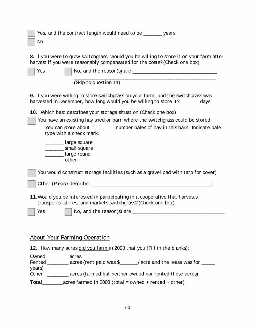
60
Yes, and the contract length would need to be _______ years No
8. If you were to grow switchgrass, would you be willing to store it on your farm after harvest if you were reasonably compensated for the costs? (Check one box)
Yes No, and the reason(s) are ________________________________ ______________________________________________________ (Skip to question 11)
9. If you were willing to store switchgrass on your farm, and the switchgrass was harvested in December, how long would you be willing to store it? _______ days
11.Would you be interested in participating in a cooperative that harvests,
transports, stores, and markets switchgrass? (Check one box)
Yes No, and the reason(s) are ___________________________________
About Your Farming Operation
12. How many acres did you farm in 2008 that you (Fill in the blanks):
Owned ________ acres Rented ________ acres (rent paid was $_______/acre and the lease was for _____ years) Other ________ acres (farmed but neither owned nor rented these acres)
Total________acres farmed in 2008 (total = owned + rented + other)
10. Which best describes your storage situation (Check one box)
You have an existing hay shed or barn where the switchgrass could be stored
You can store about _______ number bales of hay in this barn. Indicate bale type with a check mark.
_______ large square
_______ small square _______ large round _______ other
You would construct storage facilities (such as a gravel pad with tarp for cover)
Other (Please describe:______________________________________________)

61
13. Did you own additional farmland that you rented to someone else in 2008? (Check
one box)
14. If you rented
farmland to someone
else,
a) How many acres did you rent to someone else? _______ acres
b) How much rent (per acre) did you charge? $_______/acre
c) What was the length of the lease? _______ year(s)
15. How many acres of each crop/product did you grow in 2008? (Fill in the blanks)
Soybeans ______ acres Fruit ______ acres
Cotton ______ acres Vegetables ______ acres
Tobacco ______ acres Corn ______ acres
Wheat ______ acres Pasture ______ acres
Alfalfa Hay ______ acres Other Hay ______ (Describe:
______________________)
Timber ______ acres Idle ______ acres
Other Uses ______ acres (Describe:______________________________)
16.Which of the following best describes your farm’s current situation? (Check one
box) Currently have a Conservation Compliance Plan (CCP) Not required to have a CCP but practice erosion control methods
Significant erosion problems but erosion control practices not currently used No significant erosion problem on farmland
17. Do you have any acres enrolled in the Conservation Reserve Program (CRP)?
(Check one box)
18. If you have acres
enrolled in the CRP program (fill in the blank)
Grass? __________ acres Trees? __________ acres
19. Do you own any hay equipment? (Check one box)
Yes No (Skip to question 15)
Yes No (Skip to question 19)

62
20.What types of hay equipment do you own? (For each type of equipment, check one
box, then fill in the blanks)
21. Did you use custom hay harvest services in 2008? (Check one box)
22. If you used custom hay harvest services in 2008, indicate the costs per acre.(Fill
in the blanks)
Mowing/raking $_________/acre Baling for small square bales $_________/bale
Baling for round bales $_________/bale Baling for large square bales $_________/bale
23. Do you currently use no-till production methods? (Check one box) 24. Do you have any of the following types of livestock operations? (For each type of
livestock operation, check one box) Yes No Yes No
Beef cow-calf Hogs
Backgrounding/stockering Horses Dairy cattle Other (Please describe: _______________ Poultry ________________________________________)
25. Which of the following best describes your farming operation? (Check one box)
One or more of your children or grandchildren will farm your land after you
Your land will be sold for development after you cease farming
Yes No (Skip to question 21)
Yes No Mower
Rake Round Baler bale size_____________________ Small Square Baler bale size_____________________ Large Square Baler bale size_____________________ Other (Please describe: _____________________________________)
Yes No (Skip to question 23)
Yes No

63
Your land will be sold or leased to another farmer after you cease farming
Other (Please describe: _________________________________________)
26. Which of the following best describes your role in deciding which crops to grow on your farm? (Check one box)
I make the decision on my own
I share the decision making with partners or family
Someone else makes this decision
27. Which of the following best describes your farming business? (Check one box)
Sole proprietorship
A partnership
A cooperative
A corporation
Other (Please describe: _________________________________________)
28. Which of the following describes your farming operation’s net income from
farming in 2008 (before taxes)?(Check one box)
29.For every $100 of farm assets your farming operation has, how many dollars are financed with debt? (Check one box)
$0 $5-$9.99 $15-$19.99 $40-$69.99
$1-$4.99 $10-$14.99 $20-$39.99 greater than $70
30.Have you ever produced any commodity under contract? (Check one box)
Negative (less than $0) $25,000-$29,999 $50,000-$74,999
$0-$9,999 $30,000-$34,999 $75,000-$99,999
$10,000-$14,999 $35,000-$39,999 $100,000-$149,999
$15,000-$19,999 $40,000-44,999 At least $150,000
$20,000-$24,999 $45,000-49,999
Yes No

64
About You
31.Your age in years__________ Your years of experience farming _________ 32.Do you own a personal computer?(Check one box) 33.How many extension workshops or experiment station field days did you attend in
2008? (Fill in the blank) ________ 34.What is the highest education level you have attained? (Check one box)
35.What was your household’s 2008 net income (before taxes) from off-farm sources?
36. Please circle the answers that reflect your level of agreement with each of the following statements.
Statement Strongly Disagree Disagree
No Opinion Agree
Strongly Agree
You are the kind of farmer who is more willing to take financial risks than others
1 2 3 4 5
You must be willing to take substantial financial risks to be a successful farmer
1 2 3 4 5
You are reluctant about adopting new production methods or crops until you see them working for others
1 2 3 4 5
You are more concerned about a large loss to your farming operation than about missing a substantial gain
1 2 3 4 5
Yes No
Elementary/Middle school High school College graduate
Some high school Some College Post graduate
Negative (less than $0) $25,000-$29,999 $50,000-$74,999
$0-$9,999 $30,000-$34,999 $75,000-$99,999
$10,000-$14,999 $35,000-$39,999 $100,000-$149,999
$15,000-$19,999 $40,000-44,999 At least $150,000
$20,000-$24,999 $45,000-49,999

65
Part 3: AN EXCEL SPREADSHEET-BASED DECISION TOOL FOR POTIENTIAL
SWITHGRASS PRODUCERS

66
Introduction
Due to factors such as dependence on foreign oil and environmental concerns, there have
been government policy initiatives dealing with alternative fuels that have far reaching impacts
on the United States and world economies. An example of this type of policy is the Energy
Independence and Security Act (EISA) of 2007, with its key provision being the Renewable Fuel
Standard (RFS). The RFS has generated increased research into biomass production by
mandating that by at least 36 billion gallons of ethanol for fuel be produced in the United States
by 2022, with at least 16 billion gallons being ethanol that is derived from cellulose, hemi-
cellulose, or lignin (U.S. Congress 2007).
Biomass accounts for over 3 percent of the energy consumed domestically and is
currently the only source for liquid renewable fuels used in transportation (Perlack et al. 2005).
There are many sources of biomass that can be used to make solid, liquid, and gaseous fuels
including woody plants and their associated manufacturing waste and residues, aquatic plants,
biological waste, and herbaceous plants such as grasses (Mckendry 2001). Biomass is promising
because it allows us to take advantage of energy from the sun in a way that is compatible with
current technologies and can be stored without technical problems allowing its energy to be used
when needed and it could prove to be a clean energy source as the carbon that it releases during
combustion is obtained from the atmosphere, potentially making it carbon neutral.
Generating sufficient biomass to meet the EISA’s 16 billion gallon cellulosic ethanol
quota will require the production of dedicated energy crops. Switchgrass (Panicum virgatum) is
among the species of herbaceous plants being considered to help meet the expected demand
generated for biomass. Switchgrass is a warm season perennial grass. The perennial nature of

67
switchgrass separates it from more conventional annual crops because it does not have fixed
annual establishment requirements. Its native habitat includes the prairies, open ground and
wooded areas, marshes, and pinewoods of much of North America east of the Rocky Mountains
(Stubbendieck et al. 1991). There are two distinct geographic varieties or ecotypes of
switchgrass, lowland and highland (Porter 1966; Brunken and Estes 1975). Lowland types can be
found on flood plains and other areas that may be subject to flooding and upland types can
typically be found in areas that have a low potential to flood (Vogel 2004). Lowland types tend
to be taller, coarser, and show the ability to grow more rapidly than upland types (Vogel 2004).
Many benefits could be seen through the planting of switchgrass as a biomass feedstock
for fuel. Because it is a native species, it also has a natural tolerance to pest and diseases and can
be grown successfully throughout a large portion of the United States with minimal fertilizer
applications (Jensen et al. 2007), which would be cost efficient and less disruptive to the
surrounding environment. Switchgrass has the capability to show high yields on soil that, due to
low availability of nutrients or water, would not lend itself to the cultivation of conventional
crops (Lewandowski et al. 2003) which means that the grass could add utility to land that may
not be economically useful otherwise. It has the positive attribute of reducing erosion due to its
extensive root system and canopy cover (Ellis 2006) and shows the potential ability to reduce the
buildup of CO2 by being a feedstock for a cleaner burning fuel than fossil fuels and through soil
carbon sequestration due it is being a deep rooted crop (Ma et al.2000).
Despite these possible benefits that could be realized from the implementation of
switchgrass as a dedicated energy crop, there are hurdles to overcome. One of the draw backs
associated with switchgrass being produced for biomass used in energy production, being an
innovative practice, is that there is unfamiliarity associated with the specific costs of its
68
production. The decision of a farmer to adopt an innovation is based on its perceived ability to
provide more utility than other viable options which may be more conventional and whose
associated risk may be more known and understood. Because of this, the distribution of
knowledge related to the innovation, which for this study is the costs associated with the
production of switchgrass, becomes imperative to the adoption of the practice. A productive way
to disseminate this information in a manner that is readily understandable and adjustable to fit
each individual farmer’s operation is to apply it to a production decision tool in an excel
workbook.
Objective
The objective of this paper is to explicate and present an interactive and adjustable excel
spreadsheet-based decision tool for potential switchgrass producers that provides the user with
detailed information on the costs incurred in each stage of a switchgrass operation in each year of
its duration, which, for the purposes of this analysis, will be 10 years. The budget workbook is
broken down into 13 different worksheets, including:
welcome worksheet
tutorial worksheet
input-output worksheet
cash flow worksheet
cost distribution worksheet
yearly cash flow worksheet
accumulated cash flow
planting and establishment worksheet

69
stand maintenance worksheet
harvest worksheet
transportation worksheet
storage worksheet
biomass harvested worksheet
In the following chapters, the purpose of each worksheet, the source of the estimated figures in
their adjustable cells, and the methods used in their calculating cells will be explained.
Literature Review
A significant portion of literature relating to switchgrass concerns the economic aspects
of its production and delivery to a bio-refinery for the purpose of creating bio-energy. Many of
these studies are regionally (e.g. Cundiff and Marsh 1996; Epplin 1996; Larson et al. 2010a;
Larson et. al 2010b) or state (e.g. Sladden, Bransby, and Aiken 1991; Popp 2007) specific due to
the variation in suitability of the crop and the focus on biomass production for alternative fuels in
the area. Other studies focus on analyzing the cost of using switchgrass as a cellulosic biomass
feedstock in comparison to other possible grass species options (e.g. Haque et al. 2008; Wilkes
2007). The results from these studies and others like them provide information used to compose
budgets like those that create the foundation of this study.
Larson et al. (2010a), Larson et al. (2010b), Wang et al. (2009a), and Wang et al. (2009b)
are examples of studies that consider the storage cost, among other costs, and biomass losses for
different periods of storage time and methods. The data used in these studies came from a
switchgrass harvest and storage study at the Milan Research and Education Center in Milan,
Tennessee (English et al. 2008). The study analyzed many different storage options including
whether the bails were round or square, if they were placed on bare ground or on a wooden

70
pallet, the amount of time the bales were stored, and whether or not the bales were covered with
a tarp. This data has been eminently valuable to this study by providing a base useable to
calculate an estimate of the cost of storage given the type of bale used and the storage method as
well as the loss in biomass given the duration of storage.
Fulton (2010) is a study that evaluated the impacts that introducing cellulosic ethanol
plants in east Tennessee and west Tennessee would have on the economies of these two regions.
In doing this, the study analyzed the costs of transporting the switchgrass from the farm to the
bio-refinery. This information has been valuable in assembling the transportation cost section of
this study.
The Woody Biomass Program ran by the College of Environmental Science and Forestry
(ESF) at the State University of New York (SUNY) in 2008 created a Microsoft Excel based
production decision tool for growing willow (Genus: Salix) for biomass energy production called
“EcoWillow”. This willow decision tool assumed planting on marginal soils with low labor,
machinery, fertilizer, and herbicide inputs compared to traditional crops. It details the costs
associated with willow establishment, stand maintenance, harvesting, and the transportation of
the biomass. It can have a stand life of 11 or 22 years, depending on which the user chooses.
While it is useful in determining total cost estimates, it lacks the ability to estimate the cost of
storage and the amount of biomass dry matter loss during storage, both of which can factor
prominently in estimating whether or not a switchgrass stand will be a fortuitous endeavor.
Bransby et al. (2005) is a study that used Microsoft Excel to model a switchgrass budget.
It allowed for alternative producing, harvesting, handling, and transporting methods. Similar to
the Eco-Willow program created by the Woody Biomass Program at SUNY, it lacks the ability
to calculate and account for the cost of and dry matter loss during storage.

71
For any business activity, an estimated budget is needed before it is started and there are
multiple examples of budgets dealing with switchgrass operations (Wilkes 2007; Green and
Benson 2008; UT Extension 2009; UT Extension 2007). Green and Benson (2008) is a budget
put together at North Carolina State University that gives the same values for the revenues and
costs for each year of a switchgrass project. It mentions all important costs but lacks specificity
with some of the more detailed expenses. Wilkes (2007) is a budget made for the Natural
Resources Conservation Service Plant Materials Program. It estimates different costs associated
with the establishment and subsequent years, with the subsequent years having the same costs
projections. Because it covers three other grass budgets, it was not a relatively in depth analysis
of switchgrass. The University of Tennessee Extension budget (2007) and (2009) serve as
guidelines for establishing a switchgrass stand and up to ten years afterward. Most of the
recommended values for input cost in this study have been drawn from these budgets.
Case Study
For illustrative purposes, the figures in this study will represent a specific case. This case
will assume a 50 acre switchgrass stand with a mature yield of 6 dry tons of biomass per acre and
that the producer will receive 75 dollars per dry ton at the plant gate. The biomass will be stored
on farm for 200 days as round bales on pallets covered with a tarp. All other values to be used
for the case study will be the suggested University of Tennessee Extension Budget values.
Methods
Input – Output Sheet
The input-output worksheet is the most integral worksheet in this excel workbook. It ties
together the values from all of the other sheets in a way that is understandable to the user and has
macros buttons that direct the user to each respective page. The two input sections of the
72
worksheet are general data and startup loans. The output sections are financial analysis tools,
production costs, and revenues and earnings.
Input Section
The general data section (Figure 1.) has six cells where the user can insert specific data.
The interest rate for this workbook is determined in this section. The suggested interest rate is the
current thirty year Treasury bond; however, the user has the ability to input any desired rate, as
interest rates tend to fluctuate daily.
In this section, the user can input the cost of land, which includes taxes, leasing fees, and
insurance. Internal administration fees are to be included in this section, as well. There are cells
in this section that allow the user to include total acreage incentive payments they may receive
from government agencies or any other organization and their duration. The last cell in this
section gives the user the ability to insert the current price per dry ton of switchgrass at the plant
gate. The suggested price per ton is $75.00 USD.
The startup loan section (Figure 1.) contains information regarding any loans that are
taken out to establish the switchgrass stand. The three pieces of information to input are available
equity, the amount of the loan, and the interest rate. This information will be used to determine
the loan payments per period, assuming the loan is paid off over the life of the project which, in
this case, is 10 years as according to Qin et al. (2006).

73
Figure 1. The input section of the input-output sheet.
Output Section
The financial analysis tools section (figure 2.) gives output that aides the user in
understanding how the revenues and costs relate to each other over the life of the project. The
analysis includes net present value with realistic revenues and costs, net present value with
optimistic (+10% revenue and -10% costs) revenues and costs, net present value (NPV) with
pessimistic (-10% revenue and +10% costs) revenues and costs, and also gives the internal rate
of return (IRR). The formula for NPV following Ross, Westerfield, and Jaffe (2002) is as
follows:
(17) 0 + ∑
Where C0 is initial costs, T is the number of time periods of the project, t is each time period, r is
the discount rate, and Ct is the cash flow for each time period. The net present values give the

74
user an idea as to what the investment is worth in current terms after discounting each year’s
earnings back to the current period given that the project could go as planned, better than
planned, or worse than planned. The IRR is the r where
(18) 0 + ∑ = 0.
Basically, the IRR is the rate of return of a project where the NPV of the project is equal to zero.
The production costs, revenues, and earnings section (Figure 2.), like the financial
analysis tools section, is meant to aid the user in understanding the revenues and costs associated
with the project. This section contains average costs per acre, average gross revenue per acre,
average profit per acre, average revenue per ton, average costs per ton, and average earning per
ton. All of these reflect the average values over the total life of the project.
Figure 2. The output section of the input-output sheet.

75
Cash Flow Sheet
The cash flow worksheet documents the revenues and the expenditures for each year over
the life of the operation. It shows the total and per acre and per acre revenues and expenditures in
two separate diagrams. The expenditures per year include the following categories: land cost and
insurance, administration cost, planting and establishment cost, storage cost, stand maintenance
cost, harvest cost, and transportation cost. Planting and establishment costs apply only to the first
year of the project while stand maintenance, which includes the cost of reseeding applies to years
2 through 9. Included in the revenues section is the amount of money received for the biomass
and any sort of acreage incentive payments that the user might stand to receive. Finally,
expenditures are subtracted from revenues to calculate profit before the subtraction of loans,
labeled “Total Profit 1” in the table.
To put this in equation form,
(19) TotalProfit 1 Totalrevenues Totalexpenditures excluding loan payments.
In the other cost section, loan payments are calculated and subsequently subtracted from
Total Profit 1 to get profit after loan payments, which is labeled “Total Profit 2”. In equation
form, this is
(20) Total Profit 2= Total Profit 1 – loan payments
Total Profit 2 is then discounted back to the current time period for every year. This discounting
is done for the realistic revenues and costs values, the pessimistic values, and the optimistic
values. Total Profit 2 is also accumulated over each subsequent year for the realistic revenues
and costs values, the pessimistic values, and the optimistic values.

76
Figure 3. The per acre section of the cash flow sheet.
Cost Distribution
The cost distribution worksheet is meant to show the user how the costs are spread out
over the different activities associated with the production of switchgrass. It displays the land
cost and insurance, administration cost, planting and establishment cost, storage cost, stand
maintenance cost, harvest cost, and transportation cost per acre per year and in total per year. It
then displays the percent of the total costs that each activity accounts for and shows this
information in a pie chart.

77
Figure 4. The cost distribution sheet.
Yearly Cash flow
The yearly cash flow worksheet is intended to give the user a visual concept of the yearly
positive or negative undiscounted revenues. Two separate bar chart diagrams display per acre
yearly undiscounted revenues and the total yearly undiscounted revenues.
Figure 5. The per acre yearly cash flow diagram.
Accumulated Cash Flow

78
The accumulated cash flow worksheet is intended to give the user a visual idea of the
accumulated cash flows for each successive year over the life of the project. Two separate line
graphs show per acre accumulated cash flow and the total accumulated cash flow for each
successive year over the life of the project.
Figure 6. The accumulated per acre cash flow diagram.
Figure 7. NPV sensitivity analysis and NPV breakeven price.
Planting and Establishment Sheet
This sheet is designed to give the user the cost of planting and establishing his or her
switchgrass stand during the first year of the project. There are six different sections of this
worksheet including: general data, labor, travel costs, equipment, supplies, and a totals section.
79
The general data section includes acres to be planted, planting time in hours per acre, and total
planting time in hours. The number of acres to be planted comes from the value given in the
welcome sheet. Planting time is an estimate value that comes from the University of Tennessee
Extension (2009) switchgrass budget. The user has the option to change this value if a more
accurate figure is known. Total planting time is found by multiplying total acres to be planted by
planting time in hours per acre.
The labor section contains the following values: number of crew on site, laborers per
crew, laborer wage rate, hours at site per crew, indirect labor cost, the total labor cost, and the
total labor cost per acre. The number of crews on site, laborers per crew, and laborer wage rate
have values that are suggested by the University of Tennessee Extension (2009) switchgrass
budget. These values may be adjusted by the user if more accurate figures are known. The
number of hours spent at the site per crew is found by multiplying the planting time by the acres
to be planted. The total labor cost is found by multiplying the number of crews at the site, total
planting time, laborers per crew, laborer wage rate, and one plus the indirect labor cost
percentage.
The travel cost section consists of the following subsections: number of vehicles, vehicle
cost, distance, total nights, hotel cost per person per night, meal cost per day per person, and the
total travel costs. The number of vehicles, vehicle cost, distance, total nights, hotel cost per
person per night, and meal cost per person per day are adjustable values and can be altered by the
user if more accurate figures are known. The travel cost section is borrowed from the State
University of New York’s poplar excel workbook.

80
Figure 8. The general data, labor, and travel costs subsections of the planting and
establishment sheet.
The equipment section of this worksheet is divided up into 5 subsections. These
subsections are equipment delivery, tractor costs, not-till drill costs, sprayer costs, and mower
costs. The recommended values in the adjustable cells in the section come from the University of
Tennessee Extension (2009) switchgrass budget. The equipment delivery subsection contains
value cells to represent transport cost per mile for the drill, tractor, sprayer, mower, distance to
be transported, all of which are cells that allow adjustments by the user, and the total delivery
costs. The total delivery cost is determined by summing all of the transport cost per mile and
multiplying this figure by the distance both ways.

81
The tractor subsection of the equipment section contains the following value cells fixed
costs per hour, variable costs per hour, hours per acre, fixed costs per hour, variable costs per
hour, repair costs per acre, fuel costs per acre, and total tractor costs. Fixed costs per hour,
variable costs per hour, hours per acre, repair costs per acre, and fuel costs per acre are all
adjustable cells. The value for the fixed cost per acre is found by multiplying the fixed cost per
hour by the hours per acre. The value for the variable cost per acre is found by multiplying the
variable cost per hour by the hours per acre. Total tractor cost is found by multiplying the fixed
cost and the variable cost by the total acres to be planted and then adding them together.
The remaining 3 subsections in the equipment section; no-till drill cost, sprayer cost,
mower costs, have the same costs categories: fixed cost per hour, variable costs per hour, hours
per acre, fixed cost per acre, variable cost per acre, repair costs per acre, and total costs for each
respective piece of equipment. Fixed costs per hour, variable costs per hour, hours per acre, and
repair costs per acre for each respective piece of equipment are all adjustable cells. The value for
the fixed cost per acre for each piece of equipment is found by multiplying the fixed cost per
hour by the hours per acre. The value for the variable cost per acre for each piece of equipment is
found by multiplying the variable cost per hour by the hours per acre. Total cost for each piece of
equipment is found by multiplying the fixed cost and the variable cost by the total acres to be
planted and then adding them together. At the end of the equipment section the total cost of all
the equipment is calculated. This is done by adding all of the individual equipment costs
together. This total cost figure is then divided by the number of acres planted to give total
equipment costs per acre.

82
Figure 9. The equipment costs subsection of the planting and establishment sheet.
The supplies section of the planting and establishment worksheet contains three
subsections: seed costs, fertilizer costs, and burndown costs. All of the recommended values in
this section come fromthe University of Tennessee Extension (2009) switchgrass budget. The
seed costs subsection contains the price of seed per pound and the number of pounds of seed
needed per acre. The fertilizer subsection contains the phosphorus pentoxide price per pound and
pounds per acre as well as the potassium oxide price per pound and pounds per acre values. The
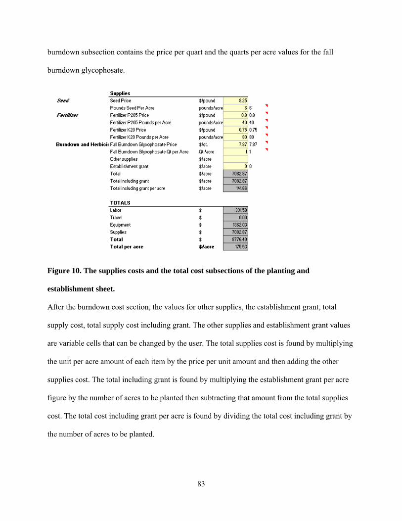
83
burndown subsection contains the price per quart and the quarts per acre values for the fall
burndown glycophosate.
Figure 10. The supplies costs and the total cost subsections of the planting and
establishment sheet.
After the burndown cost section, the values for other supplies, the establishment grant, total
supply cost, total supply cost including grant. The other supplies and establishment grant values
are variable cells that can be changed by the user. The total supplies cost is found by multiplying
the unit per acre amount of each item by the price per unit amount and then adding the other
supplies cost. The total including grant is found by multiplying the establishment grant per acre
figure by the number of acres to be planted then subtracting that amount from the total supplies
cost. The total cost including grant per acre is found by dividing the total cost including grant by
the number of acres to be planted.

84
The last section of the worksheet is the total costs section. In this section the total cost of
the planting and establishment of the project is calculated. This is done by adding the total labor,
total travel, total equipment, and total supplies costs together. The total cost per acre is found by
dividing the overall total cost by the acres to be planted.
Stand Maintenance
The stand maintenance worksheet is designed to determine the cost of maintaining the
stand of switchgrass for each year of the life of the stand after the first planting year. It contains
the following values: project size, the pounds per acre of nitrogen, the price per pound of
nitrogen, the pounds per acre of phosphorus pentoxide, the price per pound of phosphorus
pentoxide, pounds per acre of potassium oxide, price per pound of potassium oxide, spring
burndown quantity per acre, spring burndown price per acre, fall burndown quantity per acre, fall
burndown price per acre, broadleaf herbicide quantity per acre, broadleaf price per quantity,
grass herbicide quantity per acre, grass herbicide price per quantity, total stand maintenance cost,
and total stand maintenance cost per acre. All of these values, with the exception of project size,
total stand maintenance cost, and total stand maintenance cost per acre come from the University
of Tennessee Extension switchgrass budget (2007).
The values for the pounds per acre of nitrogen, the price per pound of nitrogen, the
pounds per acre of phosphorus pentoxide, the price per pound of phosphorus pentoxide, pounds
per acre of potassium oxide, price per pound of potassium oxide, spring burndown quantity per
acre, spring burndown price per acre, fall burndown quantity per acre, fall burndown price per
acre, broadleaf herbicide quantity per acre, broadleaf price per quantity, grass herbicide quantity
per acre, grass herbicide price per quantity are variable and can be changed by the user. The
estimated figures used come from the University of Tennessee Extension (2007) switchgrass

85
budget. The total stand maintenance cost per acre is found by multiplying the quantity per acre
together with the price per quantity of each item in the stand maintenance section. The total stand
maintenance cost is found by multiplying this number by the number of acres to be planted.
Figure 11. The stand maintenance sheet.
Harvest Sheet
The harvest sheet is intended to determine the total cost associated with harvesting
activities for each year of the life of the project. This sheet is broken down into five subsections
that include: general input data, labor costs, travel costs, equipment costs, totals, and costs per
ton per year. The general data section has cells for the acres to be harvested and the harvest
speed in hours per acre. The number of acres to be harvested comes from the project acres cell in
the welcome sheet. The harvest speed in hours per acre cell is an adjustable cell that allows the
user to insert his or her estimation if a more accurate one is known. The suggested value for this
cell comes from the University of Tennessee Extension (2007) switchgrass budget.

86
Figure 12. The general input, labor, and travel costs subsections for the harvest sheet.
The labor section of the harvest sheet contains nine value cells. These cells include: number of
crew on site, labors per crew, foreman per crew, laborer wage rate, foreman wage rate, hours at
site per crew, indirect labor cost, the total labor cost, and the total labor cost per acre. The
number of crews on site, labors per crew, foreman per crew, laborer wage rate, and the foreman
wage rate have values that are suggested by the University of Tennessee Extension (2007)
switchgrass budget. These values may be adjusted by the user if more accurate figures are
known. The number of hours spent at the site per crew is found by multiplying the planting time
by the acres to be planted. The total labor cost is found by multiplying together the number of

87
crews at the site, total planting time, laborers per crew, laborer wage rate, and one plus the
indirect labor cost percentage.
The travel costs section of the worksheet contains seven value cells including: number of
vehicles, vehicle cost, distance, total nights, hotel cost per person per night, meal cost per day per
person, and the total travel costs. The number of vehicles, vehicle cost, distance, total
nights,hotel cost per person per night, and meal cost per person per day all has adjustable values
and can be altered by the user if more accurate figures are known.
The equipment section of this worksheet is divided into six subsections. These
subsections are delivery cost, tractor costs, mower costs, rake costs, bailer costs, and loader
costs. The recommended values in the adjustable cells in the section come from the University of
Tennessee Extension (2007) switchgrass budget. The equipment delivery subsection contains
value cells to represent transport cost per mile for the drill, tractor, sprayer, mower, distance to
be transported; of which all are cells that allow adjustments by the user, and the total delivery
costs. The total delivery cost is found by summing all of the transport cost per mile and
multiplying this figure by the distance both ways.
The tractor subsection of the equipment section contains the following categories fixed
costs per hour, variable costs per hour, hours per acre, fixed costs per acre, variable costs per
acre, fuel costs per acre, and total tractor costs. Fixed costs per hour, variable costs per hour,
hours per acre, and fuel costs per acre are all adjustable cells. The value for the fixed cost per
acre is found by multiplying the fixed cost per hour by the hours per acre. The value for the
variable cost per acre is found by multiplying the variable cost per hour by the hours per acre.
Total tractor cost is found by multiplying the fixed cost and the variable cost per acre by the total
acres to be planted and then adding them together.

88
The four remaining subsections in the equipment section; mower costs, rake costs, bailer
cost, and loader costs, have the same costs categories: fixed cost per hour, variable costs per
hour, hours per acre, fixed cost per acre, variable cost per acre, repair costs per acre, and total
costs for each respective piece of equipment. Fixed costs per hour, variable costs per hour, hours
per acre, and repair costs per acre for each piece of equipment are all adjustable cells. The value
for the fixed cost per acre for each piece of equipment is found by multiplying the fixed cost per
hour by the hours per acre. The value for the variable cost per acre for each piece of equipment is
found by multiplying the variable cost per hour by the hours per acre. Total cost for each piece of
equipment is found by multiplying the fixed cost and the variable cost by the total acres to be
planted and then adding them together. At the end of the equipment section, the total cost of all
the equipment is calculated. This is done by adding all of the individual equipment costs
together. This total cost figure is then divided by the number of acres planted to give total
equipment costs per acre.
Below the equipment section of the harvest worksheet is the total cost section. In this
section, the total cost of the planting and establishment of the project is calculated. This is done
by adding the total labor, total travel, and total equipment costs together. The total cost per acre
is found by dividing the overall total cost by the acres to be planted.

89
Figure 13. The equipment costs and total costs subsections of the harvest sheet.
The cost per ton of harvesting per year section is the last section of the harvest worksheet.
It is intended to give the user an idea of how much of the cost per ton in each year is represented
by the cost of harvesting the biomass. The value for each year is found by dividing the total
harvest cost per year by the amount of biomass harvested in tons for each respective year.

90
Figure 14. The harvest cost per ton by year.
Transportation Worksheet
The transportation worksheet is intended to show the user the transportation costs for
each year over the life of the project. The worksheet has 13 sections that include: general data,
labor costs, equipment costs, costs in year one, costs in year two, costs in year three, costs in year
four, costs in year five, costs in year six, costs in year seven, costs in year eight, costs in year
nine, and costs in year ten.
The general data section of the worksheet contains 9 value cells including: project size
highway speed, field road speed, distance on highway (one way), distance on field road (one
way), total driving time roundtrip, loading time, unloading time, and total time per trip. Highway
speed, field road speed, distance on highway (one way), distance on field road (one way),
loading time, and unloading time are all adjustable cells that the user can change. The suggested
values for the adjustable cells in this section come from the eco-willow spreadsheet. Total
driving time round trip is calculated by multiplying the distance on the highway and the distance
on the field road by two, dividing each by the highway speed and the field road speed
respectively, and then adding these two values together. Total time per trip is found by adding
the loading time and the unloading time to the total driving time.

91
The labor costs section includes three value cells: driver wage per hour, indirect labor
costs, and average loading and unloading costs. These cells may be adjusted by the user. The
estimated value for the wage of the driver comes from Fulton (2009) and the value for the
average loading and unloading cost comes from Wang (2009).
The equipment section includes four value cells: tractor-trailer costs per mile, fuel
consumption in miles per gallon, fuel price, and maximum capacity in tons. Tractor-trailer costs
per mile, fuel consumption in miles per gallon, and fuel price are cells that allow adjusting by the
user. The estimated values for the tractor-trailer costs and fuel consumption come from Fulton
(2009). The fuel price per gallon fluctuates daily and should be changed accordingly. The
maximum capacity in tons is dependent on the type of bale used. If round bales are used, 36
bales with an average density of 0.4 tons/bale can be loaded onto each trailer. If rectangular bales
are used, 24 bales with an average density of 1 ton/bale can be loaded on a trailer. These figures
are taken from Wang (2009).
Each year of the project has a cost section to itself. Each year has the same value cells
and the values are figured in the same manner, however, different values are used for different
years. Each yearly cost section contains seven different value cells including: total trips, total
time, labor, equipment, total per acre, and total per ton. The number of total trips is calculated by
dividing the capacity of the tractor trailer by the amount of biomass mass harvested in each
respective year. Total time is found by multiplying the total number of trips by the total time per
trip. Total labor costs are found by adding average loading and unloading cost multiplied by total
trips with the product of total time and the value found by adding driver wage with driver wage
multiplied by indirect labor costs. The total equipment costs is found by multiplying together the
product of distance on field road and distance on highway, the number two, and the product of

92
the summation of tractor-trailer costs and the quotient of fuel consumption and fuel price and
total trips. Total cost is the summation of total labor and total equipment costs. Total cost per ton
is total cost divided by the tons of biomass harvested in each respective year.
Figure 15. The general data, labor costs, and equipment costs subsections of the
transportation sheet.

93
Figure 16. The yearly transportation costs of the transportation worksheet.
Storage Worksheet
The storage worksheet is designed to cover the main issues associated with the storage of
biomass. It gives the user the total loss of biomass, the total biomass that makes it to the plant
gate, and the cost of storage per ton per year. The storage worksheet contains seven sections
including: general data, bailing method, storage time, dry matter loss schedule by year in tons,
total biomass making it to the plant, and cost of storage per ton per year.
The general data section has only one data cell, which is acres planted. The value of this
cell comes from the welcome sheet. Likewise, the bailing method only has one data cell, the type

94
of bailing method to be used. This cell may be adjusted by the user, but can only take on the
value of rectangular bales or round bales. The storage time section contains three value cells,
including storage time up to 200 days, percentage going directly to plant gate, and percentage
being stored for up to 200 days. All three of these cells may be adjusted by the user by the user.
The storage method section gives the user the ability to choose which biomass storage
method he or she will be using. There are 10 storage options that include: storing large round
bales with a tarp and pallet, tarp and gravel, tarp on bare ground, pallet with no tarp, gravel with
no tarp, bare ground no tarp, storing large rectangular bales using tarp and pallet, tarp and gravel,
pallet and gravel, pallet with no tarp, and gravel with no tarp. With this spreadsheet, only one
storage option may be chosen.
Figure 17. The general data, bailing method, storage time, and storage method subsections
of the storage sheet.

95
The dry matter loss schedule by year in tons is intended to show the amount of dry matter
the user can expect to lose due to weathering and decomposition. The amount of loss incurred is
calculated by taking into consideration the percent of overall harvest that will be stored and the
amount of time that it will be stored with the amount of dry matter loss to be expected with each
storage type. The dry matter loss for each storage type comes from Wang (2009). The total
amount of biomass making it to the plant is found by subtracting the amount of loss due to
storage from the total amount harvested.
Figure 18. The dry matter loss schedule of the storage worksheet.
The total cost of storage by year section gives the total cost of storage for each year and
the total cost of storage for each year per ton. The total cost for each year has to take into account
the amount of storage materials that are still usable from the previous year in determining the
amount of material that have to be bought in each current year. Tarps, pallets, and gravel all have
different expected rates of replacement, so different storage types will have different material
rollover percentages. The amount of materials that roll over from the previous year is subtracted
from the amount that is needed in the current year to get the amount that has to be bought is the
current year.

96
Figure 19. The storage costs per year in the storage sheet.
Biomass Harvested Worksheet
The biomass harvested worksheet is designed to tell the user how much biomass he or
she can expect to get from the project in each year in total and per acre. The tons per acre value
cells may be adjusted by the user. The values used are estimates that come from the UT
switchgrass budget. With any crop, the weather and soil conditions of the region it is grown can
have a great impact on how well it performs. Therefore, it is advisable that the user tries to find
the estimated switchgrass yield for his or her area.
Figure 20. The biomass harvested sheet.

97
Conclusions
This paper explained how an adjustable excel spreadsheet decision tool for potential
switchgrass producers was made. It shows where values for costs incurred at each level of
production are derived from as well as the costs for storage and transportation of the final baled
switchgrass. A major hurdle to overcome with the production of switchgrass, as with any
innovation, is the lack of knowledge that potential adopters have about it and consequentially the
sense of risk that may accompany its implementation. This paper and the associated decision tool
have aimed at and hopefully succeeded in reducing this lack of knowledge.

98
References
Bransby D.I., H.A.Smith, C.R.Taylor, P.A. Duffy. 2005.“Switchgrass Budget Model: an
Interactive Budget Model for Producing and Delivering Switchgrass to a Bioprocessing
Plant.”Industrial Biotechnology1:122–125.
Cundiff, J. S., and Marsh, L. S. 1996. “Harvest and Storage Costs for Bales of Switchgrass in the
Southeastern United States.”Bioresource Tech. 56: 95–101.
Epplin, F.M. 1996.“Cost to Produce and Deliver Switchgrass Biomass to an Ethanol-Conversion
Facility in the Southern Plains of the United States.”Biomass and Bioenergy11(6):459–
467.
Fulton, A. 2009. “Economic Impacts of Production, Storage, Transport, and Conversion of
Switchgrass for a Cellulosic Ethanol Facility in Tennessee” MS thesis, University of
Tennessee, Knoxville.
Haque, M., F.M. Epplin, S. Aravindhakshan, and C. Taliaferro. 2008. “Cost to ProduceCellulosic
Biomass Feedstock: Four Perennial Grass Species Compared.” Selected Paperpresented
at SAEA annual meeting, Dallas, TX, February 2-6, 2008.
Larson, J.A., Mooney, D.F., English, B.C., Tyler, D.D. “Cost Analysis of AlternativeHarvest
and Storage Methods for Switchgrass in the Southeastern U.S.” 2010 AnnualMeeting of
Southern Agricultural Economics Association, Orlando FL, February 6-9.
Larson, J.A., T. H. Yu, B. C. English, D. F. Mooney, C. Wang. 2010. “Cost Evaluation of
Alternative Switchgrass Producing, Harvesting, Storing, and Transporting Systems and
their Logistics in the Southeastern U. S.” Submitted for publication to the Agicultural
Finance Review.
McKendry,P. 2002. “Energy Production from Biomass (Part 1): Overview of
Biomass.”Bioresource Technology 83:37–46.

99
McLaughlin, S. B., and L. A. Kszos. 2005. “Development of Switchgrass (Panicum virgatum) as
a Bioenergy Feedstock in the United States.” Biomass & Bioenergy 28(6):515-535.
Monti A, S. Fazio, V. Lychnaras, P. Soldatos, G. Venturi. 2005.“A full Economic Analysis of
Switchgrass Under Different Scenarios in Italy Estimated by BEE Model. Biomass &
Bioenergy 31:177–185.
Natural Resources Conservation Service Plant Materials Program. 2007. “Estimated Production
Cost Budgets For Biomass: Switchgrass, Highlander Eastern Gamagrass, Indiangrass,
and Big Bluestem.” Jackson MS, May.
North Carolina State University Extension. 2008. “Switchgrass for Biomass for Energy
Production: Estimated Annual Revenue, Operating cost, Fixed Cost and Net Returns per
Acre.” Raleigh NC, July.
Popp, M. 2007. “Assessment of Alternative Fuel Production from Switchgrass: An Example
from Arkansas.” Paper presented at the Southern Agricultural Economics Association
meetings in Mobile AL, Feb. 3-8.
Qin, X., T. Mohan, M. El-Halwagi, G. Cornforth, B. McCarl. 2006.“Switchgrass as an Alternate
Feedstock for Power Generation: an Integrated Environmental, Energy and
Economic Life-cycle Assessment.”Clean Technologies and Environ Policy
8:233–249.
Ross, S. A., R. W. Westerfield, and J. F. Jaffe. 2005. Corporate Finance, 3rded., Irwin Publishers.
Sladden, S. E., Bransby,D. I., and Aiken, G. E. 1991. “Biomass Yield, Composition and
Production Costs for Eight Switchgrass Varieties in Alabama.”Biomass andBioenergy
1(2):119–122.
100
U. S. Congress, House of Representatives. 2007. Energy Independence Act of 2007. Washington
D.C.: House Document 6, 100th Cong., 1st Sess., 4 January.
University of Tennessee Extension Agency. 2009. “Guideline Switchgrass Establishment and
Annual Production Budgets Over Three Year Planning Horizon.” Knoxville TN, July.
University of Tennessee Extension Agency. 2007. “Guideline Switchgrass Establishment and
Annual Production Budgets Over Three, Six, and Ten Year Planning Horizons.”
Knoxville TN, October.
Wang, C. 2009 “Economic Analysis of Delivering Switchgrass to a Bio-refinery From Both the
Farmers’ and Processor’s Perspectives.” MS thesis, University of Tennessee, Knoxville.
Wang, C., J.A. Larson, B.C. English, K. Jensen. “Cost Analysis of Alternative Harvest, Storage
and Transportation Methods for Delivering Switchgrass to a Bio-refinery from the
Farmers’ Perspective.” 2009. Paper presented at the Southern Agricultural Economics
Association Annual Meeting, Atlanta GA, Jan. 31- Feb. 3.

101
Part 4: Conclusions
102
Conclusions
This study analyzed the influences that various socioeconomic and farm characteristics have on
producers’ interest in growing and the extent to which they would be willing to produce
switchgrass given different plant gate prices. The results of this study have several possible
implications for switchgrass production and adoption expansion efforts in the southeastern
United States. Based on the results, individuals and organizations that want to promote interest in
adopting switchgrass may want to emphasize switchgrass’ positive attributes, such as its
potential for lowering input requirements, its ability to diversify a producer’s crop mix, and the
possibility of it contributing to the nation’s energy security and environment. Also, farmers that
have erosion problems on their land showed higher interest in switchgrass production, which
means that switchgrass’ ability to reduce erosion compared to more traditional crops could be
emphasized as well. Concerns that affect producers’ interest in growing switchgrass that likely
need to be addressed through educational programs include management techniques to deal with
possible conflicts between the planting and harvesting of switchgrass and other crops, contract
arrangements that enable planting of switchgrass on land that is leased, and efficient use of
financial and equipment resources needed to produce switchgrass.
From the results, it can be concluded that older producers would be less interested in
switchgrass production, as they may not continue farming long enough to see the full benefits of
a switchgrass stand. Those producers that operate a beef cattle operation are likely to be less
interested, as well. This may be due to the reluctance of these producers to convert acres of
pasture to switchgrass production and seems to indicate that areas with a high percentage of beef
cattle farmers may not be an ideal switchgrass production area. Contrarily, producers that own
hay equipment or have used custom hay harvest service may be more likely to be interested in

103
growing switchgrass. Hence, switchgrass may be first adopted by producers who already have
equipment that may be helpful in growing switchgrass.
The results of this study indicate that the share of acres that would be converted to
switchgrass will be less on a larger farm. Also, while older farmers may be less willing to adopt
switchgrass, those that do may be willing to devote more acreage that a younger farmer. This
indicates that areas with smaller farms and younger farmers, on average, may show more acres
being converted to switchgrass, ceteris paribus. Those producers who are reluctant to adopt a
new crop before they see it work for others reasonably may show less interest in producing
switchgrass and if they are willing to adopt, will likely convert a smaller share of acreage to
switchgrass. Producers with a higher percentage of acreage devoted to CRP land may show a
likelihood of devoting a smaller share of acres to switchgrass, which indicates that areas with
producers that have a higher portion of their land devoted to CRP may devote a smaller portion
of acres to switchgrass. This result suggests that CRP rules may need to be modified to
encourage switchgrass production in a sustainable way on CRP lands. The results show that
producers are sensitive to price with respect to both adopting switchgrass and the share of acres
they would be willing to convert, indicating that a higher price offered at the plant gate should
mean that a bio-refinery will receive more biomass.
This study has given new information about switchgrass production from the producer’s
prospective in the southeastern U. S. However, there is still a substantial lack of knowledge in
related areas, such as contract preferences or harvesting and storage arrangements, that future
studies can build upon.

104
This paper also explained how an adjustable excel spreadsheet decision tool for potential
switchgrass producers was put together. It showed where values for costs incurred at each level
of production are derived from as well as the costs for storage and transportation of the final
baled switchgrass. It addresses a major hurdle with the production of switchgrass, as with any
innovation, the one of lack of knowledge that potential adopters have about it and the risk that
accompanies this perceived risk. This paper and the associated decision tool aimed at and
hopefully succeeded in reducing this lack of knowledge.

105
Vita
Donald Joshua Qualls was born in Dyersburg, Tennessee on February 19, 1987. He
graduated from Obion County Central High School in 2005. In the fall of the same year, he
enrolled in the University of Tennessee at Martin where he graduated with a Bachelors of
Science in Agriculture Business in December of 2008. In August of 2009 he entered the Master
of Science program in Agricultural Economics at the University of Tennessee at Knoxville. He
completed the Master of Science degree in May of 2011.