San Jose State University San Jose State University

SJSU ScholarWorks SJSU ScholarWorks

Master's Projects Master's Theses and Graduate Research

Spring 2018

Analysis of Encrypted Malicious Traffic Analysis of Encrypted Malicious Traffic

Anish Singh Shekhawat San Jose State University

Follow this and additional works at: https://scholarworks.sjsu.edu/etd_projects

Part of the Computer Sciences Commons

Recommended Citation Recommended Citation Shekhawat, Anish Singh, "Analysis of Encrypted Malicious Traffic" (2018). Master's Projects. 622. DOI: https://doi.org/10.31979/etd.ufky-m35f https://scholarworks.sjsu.edu/etd_projects/622

This Master's Project is brought to you for free and open access by the Master's Theses and Graduate Research at SJSU ScholarWorks. It has been accepted for inclusion in Master's Projects by an authorized administrator of SJSU ScholarWorks. For more information, please contact scholarworks@sjsu.edu.

Analysis of Encrypted Malicious Traffic

A Project

Presented to

The Faculty of the Department of Computer Science

San José State University

In Partial Fulfillment

of the Requirements for the Degree

Master of Science

by

Anish Singh Shekhawat

May 2018

© 2018

Anish Singh Shekhawat

ALL RIGHTS RESERVED

The Designated Project Committee Approves the Project Titled

Analysis of Encrypted Malicious Traffic

by

Anish Singh Shekhawat

APPROVED FOR THE DEPARTMENT OF COMPUTER SCIENCE

SAN JOSÉ STATE UNIVERSITY

May 2018

Dr. Mark Stamp Department of Computer Science

Dr. Katerina Potika Department of Computer Science

Fabio Di Troia Department of Computer Science

ABSTRACT

Analysis of Encrypted Malicious Traffic

by Anish Singh Shekhawat

In recent years there has been a dramatic increase in the number of malware

attacks that use encrypted HTTP traffic for self-propagation and communication.

Due to the volume of legitimate encrypted data, encrypted malicious traffic resembles

benign traffic. As the malicious traffic is similar to benign traffic, it poses a challenge

for antivirus software and firewalls. Since antivirus software and firewalls will not

typically have access to encryption keys, detection techniques are needed that do not

require decrypting the traffic. In this research, we apply a variety of machine learning

techniques to the problem of distinguishing malicious encrypted HTTP traffic from

benign encrypted traffic.

ACKNOWLEDGMENTS

I would like to express my sincere gratitude to my advisor, Dr. Mark Stamp, for

his encouragement, patience, and continuous guidance throughout my project and

graduate studies as well. I would also like thank my committee members Dr. Katerina

Potika and Fabio Di Troia for reviewing my work and providing valuable feedback.

I am also grateful to my family and friends who have supported me throughout

the course of my Masters program.

v

TABLE OF CONTENTS

CHAPTER

1 Introduction . . . . . . . . . . . . . . . . . . . . . . . . . . . . . . . . 1

2 Related Work . . . . . . . . . . . . . . . . . . . . . . . . . . . . . . . 3

3 Dataset . . . . . . . . . . . . . . . . . . . . . . . . . . . . . . . . . . . 6

3.1 Data Structure . . . . . . . . . . . . . . . . . . . . . . . . . . . . 7

3.2 Feature Extraction . . . . . . . . . . . . . . . . . . . . . . . . . . 7

3.3 Features . . . . . . . . . . . . . . . . . . . . . . . . . . . . . . . . 9

3.4 Labels . . . . . . . . . . . . . . . . . . . . . . . . . . . . . . . . . 9

4 Methodolgy . . . . . . . . . . . . . . . . . . . . . . . . . . . . . . . . 13

4.1 Machine Learning . . . . . . . . . . . . . . . . . . . . . . . . . . . 13

4.1.1 Support Vector Machines . . . . . . . . . . . . . . . . . . . 13

4.1.2 Random Forest . . . . . . . . . . . . . . . . . . . . . . . . 15

4.1.3 XGBoost . . . . . . . . . . . . . . . . . . . . . . . . . . . . 16

4.1.4 Cross-Validation . . . . . . . . . . . . . . . . . . . . . . . 17

4.2 Evaluation Metrics . . . . . . . . . . . . . . . . . . . . . . . . . . 18

5 Experiments . . . . . . . . . . . . . . . . . . . . . . . . . . . . . . . . 19

5.1 Training Experiments . . . . . . . . . . . . . . . . . . . . . . . . . 19

5.2 Data Analysis . . . . . . . . . . . . . . . . . . . . . . . . . . . . . 19

5.3 K-means Clustering . . . . . . . . . . . . . . . . . . . . . . . . . . 20

5.4 Experiments . . . . . . . . . . . . . . . . . . . . . . . . . . . . . . 24

5.4.1 SVM with 10-fold cross validation . . . . . . . . . . . . . . 24

vi

vii

5.4.2 SVM with different kernels . . . . . . . . . . . . . . . . . . 25

5.4.3 Univariate Feature Elimination . . . . . . . . . . . . . . . 25

5.4.4 SVM with Recursive Feature Elimination . . . . . . . . . . 26

5.4.5 Random Forest . . . . . . . . . . . . . . . . . . . . . . . . 27

5.4.6 XGBoost . . . . . . . . . . . . . . . . . . . . . . . . . . . . 28

5.4.7 Classification based on malware family . . . . . . . . . . . 30

5.5 Discussion . . . . . . . . . . . . . . . . . . . . . . . . . . . . . . . 34

6 Conclusion and Future Work . . . . . . . . . . . . . . . . . . . . . 39

6.1 Conclusion . . . . . . . . . . . . . . . . . . . . . . . . . . . . . . . 39

6.2 Future Work . . . . . . . . . . . . . . . . . . . . . . . . . . . . . 40

LIST OF REFERENCES . . . . . . . . . . . . . . . . . . . . . . . . . . . 41

LIST OF TABLES

1 Dataset Statistics . . . . . . . . . . . . . . . . . . . . . . . . . . . 7

2 Extracted features from conn.log . . . . . . . . . . . . . . . . . . 10

3 Extracted Features from ssl.log . . . . . . . . . . . . . . . . . . . 11

4 Extracted Features from x509.log . . . . . . . . . . . . . . . . . . 12

5 Top Five Ports Used by ORIG . . . . . . . . . . . . . . . . . . . 20

6 Top Five Ports Used by RESP . . . . . . . . . . . . . . . . . . . 22

7 Top 20 Feature ranks by SVM . . . . . . . . . . . . . . . . . . . 26

8 Malware Family Dataset . . . . . . . . . . . . . . . . . . . . . . 32

viii

LIST OF FIGURES

1 Interconnection of log records using unique keys in Bro . . . . . . 8

2 SVM hyperplane and support vectors . . . . . . . . . . . . . . . . 14

3 SVM maps input data to feature space . . . . . . . . . . . . . . . 15

4 Random Forest . . . . . . . . . . . . . . . . . . . . . . . . . . . . 15

5 10-fold cross-validation. The red rectangle is the testing set and theother subsets are used for training. . . . . . . . . . . . . . . . . . 18

6 Frequency of ports used by ORIG . . . . . . . . . . . . . . . . . . 20

7 Frequency of ports used by RESP . . . . . . . . . . . . . . . . . . 21

8 Original Scatter Plot vs K-means clustering . . . . . . . . . . . . 23

9 Original Scatter Plots with different axes . . . . . . . . . . . . . . 23

10 SVM with 10-fold cross-validation . . . . . . . . . . . . . . . . . . 24

11 Weights assigned to features by SVM . . . . . . . . . . . . . . . . 25

12 SVM with different kernels . . . . . . . . . . . . . . . . . . . . . 27

13 Weights assigned to the features by SVM and UFE . . . . . . . . 28

14 Recursive Feature Elimination with SVM . . . . . . . . . . . . . 29

15 Recursive Feature Elimination with Random Forest . . . . . . . . 30

16 Random Forest feature importance . . . . . . . . . . . . . . . . . 31

17 Random Forest with different number of estimators . . . . . . . . 32

18 XGBoost with Recursive Feature Elimination . . . . . . . . . . . 33

19 XGBoost feature importance . . . . . . . . . . . . . . . . . . . . . 34

20 XGBoost with different number of estimators . . . . . . . . . . . 35

ix

x

21 Performance comparison of the three machine learning algorithms 35

22 Performance comparison of the three machine learning algorithmsfor malware family based classification . . . . . . . . . . . . . . . 36

23 Performance comparison of the three machine learning algorithmsfor multi-class problem . . . . . . . . . . . . . . . . . . . . . . . . 37

24 Comparison of various machine learning algorithms . . . . . . . . 37

25 Feature correlation heat map . . . . . . . . . . . . . . . . . . . . 38

CHAPTER 1

Introduction

Malware is, arguably, the greatest threat to information security today. Malware,

short for malicious software is a computer program designed to infiltrate and damage

or disable computer systems without the user’s consent [1]. These malicious programs

often communicate with a command and control (C&C) server to fetch commands

from an attacker. According to Malwarebytes, a popular cybersecurity product, over

90% of small-to-medium sized businesses (SMB) have experienced an increase in the

number of malware detection---some businesses experienced an increase of 500% in

March 2017 alone [2]. Real-time malware detection using network traffic information

has the potential to prevent---or at least greatly reduce---malware propagation on the

network.

One approach to detect network traffic is to use deep packet inspection for

investigating the contents and intent of the network traffic. Such techniques aggregate

successive packets that have the same protocol type and same source and destination

port and address. They then analyze the contents of these aggregated packets and

check for signatures that have been previously discovered to classify the source as

malicious or benign [3].

Unfortunately, due to the widespread use of the HyperText Transfer Protocol

Secure (HTTPS), or HTTP over Secure Socket Layer (SSL), such deep packet inspec-

tion methods can be inadequate to classify the network traffic. HTTPS is a secure

communication protocol and, according to Google, more than 70% of internet traffic

is using HTTPS to communicate over the Internet [4].

HTTPS is, essentially, HTTP using either the Secure Sockets Layer (SSL) or

Transport Layer Security (TLS). Unencrypted traffic is exposed and can be read

by anyone who can intercept the traffic packets. As everyday objects become more

1

digital, many software applications and internet connected devices use encryption

as their primary method to protect privacy, secure communications and maintain

trust over the Internet. As a result, the rise in encrypted network traffic has affected

the cybersecurity landscape. Malware can also leverage encryption by using it to

evade detection and hide malicious activities. CISCO released a report [5] which

states that although a majority of malware do not encrypt their network traffic, there

is a steady 10% to12% increase annually in malicious network traffic that encrypt

their communication using HTTPS. The 2017 Global Application & Network Security

Report from Radware [6], a leading cyber security and application delivery firm, states

that 35% of the organizations in their global security survey faced TLS or SSL based

attacks, which represents an increase of 50% over the previous year.

The main purpose of this research is to analyze whether we can effectively

distinguish encrypted malicious network traffic from encrypted benign traffic, without

decrypting. This paper is focused on the use of machine learning as a possible solution

to this problem. Specifically, we use machine learning to analyze encrypted network

traffic based on a wide variety of unencrypted information, such as connection duration,

source and destination ports and IP addresses, SSL certificate key lengths, and so on.

The remainder of the paper is organized as follows. Chapter 2 gives a basic

overview of previous work related to the problem of detecting malicious traffic. In

Chapter 3, we discuss the datasets used in our experiments. Chapter 4, discusses

the proposed methodology. Chapter 5 gives our experimental results and analysis.

Finally, in Chapter 6, we give our conclusion and briefly discuss future work.

2

CHAPTER 2

Related Work

Traditional malicious network communication techniques rely either on port-

based classification or deep packet inspection and signature matching techniques.

Port-based methods rely on inspection of Transmission Control Protocol (TCP) or

User Datagram Protocol (UDP) port numbers [7] and assumption that applications

always use well-known port numbers that are registered by the Internet Assigned

Numbers Authority (IANA) [8]. Dreger and Feldmann in [9] showed that malicious

applications use non-standard ports to evade network intrusion detection systems

(NIDS) and restricting firewalls. Even prominent applications such as Skype use

dynamic port numbers to escape restrictive firewalls [10]. Madhukar and Williamson

in [11] showed that port-based classification mis-classifies network flow traffic 30-70%

of the time.

Etienne in [12] used deep packet inspection to detect malicious traffic by in-

specting payload contents and using traditional pattern matching or signature based

techniques. Etienne used Snort [13], an intrusion detection application, to detect

malicious traffic using signature or string matching on the packet contents. Snort

also hosts a popular Intrusion Protection System (IPS) rule set maintained by the

community [14]. But only around 1 % of the rule set are TLS specific which shows that

traditional pattern matching techniques are not used often for TLS based malware.

Sen et al. [3] demonstrates the use of deep packet inspection to reduce false positive

and false negative rates by 5% when classifying Peer-to-Peer (P2P) traffic. Moore and

Papagiannaki in [15] achieved a 100% accuracy when identifying network applications

using the entire packet payload. The primary limitations of these methods are the

invasion of user privacy and the huge overhead of decrypting and analyzing each

packet.

3

Tegeler et al. in [16] presented BotFinder, a network-flow information based

system to detect bot infections. The system uses a sequence of chronologically-ordered

flow called traces to find irregularities in the network behavior between two endpoints.

This along with other network metadata such as average time interval, averaged

duration, average number of source and destination bytes, etc. were used as features

in a local shrinking based clustering algorithm [17]. Prasse et al. in [18] derived a

neural network based malware detection using network flow features such as port

value, connection duration, number of bytes sent and received, time interval between

packets and domain name features. We do not use domain name features or Domain

Name System (DNS) data as features due to the introduction of DNS over TLS where

the DNS data is also encrypted using TLS [19]. Lokoč et al. in [20] presented a k-NN

based classification technique that could identify servers contacted by malware using

HTTPS traffic.

Anderson and McGrew in [21] proposed a new technique that analyzed network

flow metadata and applied supervised machine learning algorithms to identify en-

crypted malware traffic. They used a demilitarized zone (DMZ), to collect and train

the machine learning algorithm on the benign network traffic. DMZ is a sub-network

that separates the externally connected services from internal systems. Externally

connected services are those which connect to the internet to provide various services.

As it was based on supervised learning models, it provided results which can be

easily interpreted [22]. The machine learning model helped in high-speed processing

of the network traffic and real-time predictions. It also leveraged regularization, an

important part of training, to select features that are most discriminatory [23]. Since

the DMZ segregates such services and is used only in business organizations, the

network traffic data collected by them is not an actual representation of the general

network traffic. Since this data represents only enterprise users, i.e. those who work

4

in business organizations, the results may not hold for general internet users such as

students or home users as mentioned in [21].

This paper further explores the use of various network flow information as features

to train machine learning algorithms. These features are obtained without decrypting

any packets in the network flow. The paper also explores the use of these features to

classify malicious traffic based on malware family and discussed the importance of

these features using various machine algorithms algorithms.

5

CHAPTER 3

Dataset

One of the most important step of a machine learning design methodology is

the collection of dataset that represents the problem we wish to solve. We used two

popular and published network capture dataset that contains malware and benign

traffic.

• CTU-13 Dataset [24]

The CTU-13 dataset was captured in the Czech Technical University, Czech

Republic. It is a set of 13 different malware traffic captures which includes

normal, malware and background traffic. Each malware traffic was captured by

executing the malware in a Windows virtual machine and recording the network

traffic on that host. The normal traffic corresponds to network traffic which

was captured on normal hosts, i.e. hosts which weren’t infected with malware.

We will only be using only normal and malware traffic which are stored in pcap

files.

• Malware Capture Facility Project [25]

This research project is also carried out at Czech Technical University ATG

Group to capture, analyze and publish long-lived real malware network traffic.

The dataset was contributed by Maria Jose Erquiaga. The malware was executed

with two restrictions: a bandwidth limit and spam interception. The most

important characteristic of this project is the execution of malware during long

periods of time, that can go up to several months. The traffic is stored in pcap

files, labeled and made public for the research community

The entire dataset consists of total 72 captures out which 59 are malware captures

and 13 are benign captures. Table 1 gives us basic statistics about our dataset.

6

Table 1: Dataset Statistics

Total Number of connection 4-tuples 61726Number of normal 4-tuples 8828Number of malware 4-tuples 52898Total number of flows 1136631Normal flows 69358Malware flows 1067273

3.1 Data Structure

Each dataset contains a pcap file of the capture, list of infected and normal hosts

and Bro IDS logs generated using the pcap files. Bro [26] is a powerful open-source

network analysis and intrusion detection tool. It supports various network analysis

features traffic inspection, log recording, attack detection, etc. We use Bro to generate

various network traffic logs which describe the network flow information and other

metadata. This information is then used to extract various features about the traffic

flow and use the those features to train and test machine learning models. Bro

generates various log files but we are mainly interested on the following three log files:

1. conn.log : It contains information about TCP, UDP and ICMP connections.

2. ssl.log: It contains information about SSL/TLS certificates and sessions.

3. x509.log: It contains information about X.509 certificates.

3.2 Feature Extraction

We extracted several features from the Bro logs generated using the network

captures. Features related to a single connection is spread over different log files.

For example, if we have an SSL connection to some server, the connection features

such as source, destination IP addresses, ports, protocols, connection duration, etc.

are stored in connection log (conn.log). The SSL features such as cipher used, server

7

name, etc. are stored in SSL log (ssl.log) and certificate features such as key lengths,

common names, validities, subjects, etc. are stored in certificate logs (x509.log).

Bro provides interconnection between various logs using unique keys. These unique

keys are common for a connection across different logs provided by Bro as shown in

Figure 1. Hence, an SSL connection will have the same unique key to identify the

record in connection and SSL logs. SSL has certificate ids to uniquely identify x509

certificates in certificate logs which were used in the SSL session or connection.

(a) conn.log

(b) ssl.log

(c) x509.log

Figure 1: Interconnection of log records using unique keys in Bro

Bro tracks every incoming and outgoing connection in conn.log. Every record

in the conn.log gives us information about a particular connection. Since we are

interested only in encrypted network connection, i.e. HTTPS, we only consider

connection records that are related to HTTPS connections. Since HTTPS connection

uses SSL/TLS to protocols to establish an encrypted link between the client and the

server, we only extract connection records which have corresponding entries in the

ssl.log file. This can be achieved by going through all the records in ssl.log file and

extracting corresponding connection records from the conn.log file.

Since, every SSL/TLS connection requires a server certificate to ensure credibility

of the server [27], every record in ssl.log contains one or more than one unique certificate

8

ids that the server offered to validate its signing chain. The unique certificate ids

represent the certificate record in the x509.log file. We extract only the first certificate

id from the ssl.log file since it corresponds to the end-user certificate. The remaining

ids correspond to intermediate and root certificates.

Every connection record can be identified by the 4-tuple of source IP address,

destination IP address, destination port and protocol. We use this 4-tuple as key to

aggregate network features. Hence every connection which has the same 4-tuple key

is grouped together. We then extract features from each group of connection records

which were aggregated in the previous step.

3.3 Features

We extracted some features based on [28, 29] from the connection, SSL and

certificate log files from Bro. Table 2 contains connection features extracted from

conn.log, Table 3 contains SSL features extracted from ssl.log and Table 4 contains

certificate features extracted from x509.log. All the features are computed over a

single connection 4-tuple aggregate of records.

3.4 Labels

The dataset from [24] and [25] contains IP addresses of infected and normal hosts.

We use these IP addresses to label our dataset accordingly. Hence, if a connection

record has an infected IP address either as source or destination then the record is

classified as malware else it is classified as benign.

9

Table 2: Extracted features from conn.log

S.No Feature Name Description1 no_of_flows Number of aggregated records in connection

4-tuple2 avg_of_duration Mean duration of connections3 standard_deviation_of_duration Standard deviation of connections4 percent_sd_of_duration Percentage of records with duration greater

than standard deviation5 size_of_orig_flows No. of bytes sent by the originator6 size_of_resp_flows No. of bytes sent by the responder7 ratio_of_sizes Ratio of responder bytes by all bytes trans-

mitted8 percent_of_established_conn Percentage of established connections out

of all attempted connections9 inbound_pckts No. of incoming packets10 outbound_pckts No. of outgoing packets11 periodicity_average Mean of periodicity of connection12 periodicity_standart_deviation Standard deviation of periodicity of connec-

tion

10

Table 3: Extracted Features from ssl.log

S.No Feature Name Description1 ssl_ratio Ratio of SSL records to non-SSL records2 tls_version_ratio Ratio of records with TLS3 SNI_ssl_ratio Ratio of connections having Server Name

Indication (SNI) in SSL record4 self_signed_ratio Ration of connection with self signed cer-

tificates5 SNI_equal_DstIP 1 if SNI is equal to destination IP in SSL

record6 differ_SNI_in_ssl_log Ratio of SSL records with different SNI7 differ_subject_in_ssl_log Ratio of SSL records with different subjects

than certificate8 differ_issuer_in_ssl_log Ratio of SSL records with different issuer

than certificate9 ratio_of_same_subjects Ratio of SSL records with same subject as

certificate10 ratio_of_same_issuer Ratio of SSL records with same issuer as

certificate11 is_SNI_top_level_domain 1 if SNI is a top level domain12 ratio_missing_cert Ratio of records with missing certificates

11

Table 4: Extracted Features from x509.log

S.No Feature Name Description1 avg_key_len Average cipher key length2 avg_of_certificate_len Average certificate length3 standart_deviation_cert_len Standard deviation of certificate length4 is_valid_certificate 1 if the certificate is valid during capture5 amount_diff_certificates No. of different certificates6 no_of_domains_in_cert No. of domains in certificates7 certificate_ratio Ratio of certificates validity time lengths8 no_of_cert_path No. of signed certificates paths9 x509_ssl_ratio Ratio of SSL logs with x509 certificates10 is_SNIs_in_SAN_dns Checks if SNI is SAN DNS11 is_CNs_in_SAN_dns 1 if all certificates have Comman Names in

SAN12 differ_subject_in_cert Ratio of different subject in certificates13 differ_issuer_in_cert Ratio of different issuer in certificates14 differ_sandns_in_cert Ratio of different SAN DNS in certificates15 is_same_CN_and_SNI Checks if CN is same as SNI16 average_certificate_expo Average of certificate exponent17 ratio_certificate_path_error Checks if certificate path is valid

12

CHAPTER 4

Methodolgy

An important part of any machine learning based detection technique is to choose

the most effective machine learning algorithm. For our experiments, we will use

various algorithms and try to find the one with the highest accuracy.

4.1 Machine Learning

Machine learning is a field of computer science that helps us automate the process

of learning from the data. It helps computers to learn and act without any human

intervention [30]. The process of learning from the data can be broadly divided into

two parts:

• Supervised Learning: In this the computer is given input data along with the

desired outputs and the aim is to learn a function that maps the input data to

the desired values.

• Unsupervised Learning: In this the computer is given only input data without

any labels or desired outputs and asked to either predict new data or classify

the given input data into separate classes.

In our research we labeled the input data as mentioned in Chapter 3 and thus

know if a particular connection is malicious or benign. Since we already know the

labels of the input data, we use supervised learning algorithms such as Support Vector

Machine (SVM), Random Forest, XGBoost and Deep learning based algorithms to

train our machine learning models on the input data.

4.1.1 Support Vector Machines

Support Vector Machine (SVM) is a supervised learning algorithm that outputs

an optimal separating hyperplane given labeled training data. This hyperplane is

then used to classify new samples. The hyperplane is defined by a small subset of the

training the training data known as support vectors as shown in Figure 2.

13

Figure 2: SVM hyperplane and support vectors

SVM is based on the following three concepts:

• Margin Maximization: SVM maximizes the margin, i.e. the distance between

the support vectors to find the optimal hyperplane as shown in Fig 2

• Works in Higher Dimension Space: If the training data is not linearly separable,

SVM maps the input data to a higher dimensional feature space in which the

data is linearly separable as shown in Figure 3.

• Kernel Trick: While maximizing the separation margin we do not need the exact

points in the higher dimension feature space, but need only their inner products.

Getting the inner product is much easier than getting actual points in a higher

dimension space. The Kernel trick helps us to operate in a high-dimensional

feature space without computing the coordinates of the input data in feature

space.

One of the advantages of SVM is its effectiveness in high dimensional spaces such

as our own data where we have 41 features. Hence, it was a primary choice for our

experiments.

14

Figure 3: SVM maps input data to feature space

4.1.2 Random Forest

Random Forest is a supervised learning algorithm that is used in classification

and regression. It builds an ensemble of decision trees and merges them together to

get a stable and more accurate prediction [31]. As seen in Figure 4 [32], Random

Forest uses bootstrap aggregation also known as bagging to combine predictions from

multiple decision trees together to make a more accurate prediction. This reduces the

variance of the model without increasing the bias.

Figure 4: Random Forest

15

Random Forest is created using the following steps:

1. ’K’ features are randomly selected from a total of ’m’ features such that K<< m

2. Using the ’K’ features a decision tree node is selected using the best split point.

3. The selected node is further split into child nodes using the best split.

4. Steps 1-3 are repeared until number of nodes is 1.

5. Decision tree forest is build by repeating Steps 1-4 for ’n’ number of times

As shown in Figure 4, the algorithm follows steps mentioned below to predict

the class of the test sample.

1. It takes the features of the test sample and goes through each decision tree to

predict the outcome.

2. Calculates the number of votes for each predicted class.

3. Declares the highest voted class as the final prediction.

4.1.3 XGBoost

XGBoost (eXtreme gradient boosting) is a relatively new software library which

was initially started by Tianqi Chen [33, 34] as a research project. It is based upon

gradient boosting which is an old machine learning technique used for regression

and classification. Like Random Forest, gradient boosting technique also outputs an

ensemble of weak decision trees as a prediction model.

Gradient boosting and Random Forest both use ensemble methods, i.e. building a

strong classifier from many weak classifiers. But, the fundamental difference between

the two algorithms lies in the methods used to build the strong classifier. Gradient

boosting builds on weak classifier sequentially, i.e. one classifier is added at a time

16

which improves upon the already trained ensemble. Whereas in Random Forest

bagging is used to create a large number of weak classifiers in parallel, i.e. the classifier

is trained independently from the rest.

In mathematical terms, if the ensemble has three trees, the prediction model can

be given asD(x) = dtree1(x) + dtree2(x) + dtree3(x)

According to gradient boosting the next tree would improve upon the already trained

ensemble by minimizes the training error. Thus, the new model D′(x) can then be

given asD′(x) = D(x) + dtree4(x)

4.1.4 Cross-Validation

Cross-validation is a technique to evaluate how machine learning models perform

on a given dataset. It is mainly used in situations such as ours where there is not

enough data to divide the dataset into separate training and testing sets. Cross

validation can be divided into two types:

• Exhaustive cross-validation: In this cross-validation method we learn and test

on all possible combinations of the training and testing set.

– Leave-p-out: Leave-p-out is a type of exhaustive cross-validation where we

use p sets as validation set and the remaining are used as training set.

• Non-exhaustive cross-validation: In this cross-validation method we do not

compute all possible combinations of the training and testing set.

– Holdout method: This is the simplest cross-validation method where the

dataset is separated into two sets, the training and testing set.

– k -fold cross-validation: In this cross-validation method we divide the

dataset into k subsets and then the model is iteratively tested on one set

and trained on the remaining set.

17

We use 10-fold cross-validation in all our experiments. As shown in Figure 5, our

dataset is divided into ten subsets and the model is then iteratively trained on nine

subsets and tested on one subset.

Figure 5: 10-fold cross-validation. The red rectangle is the testing set and the othersubsets are used for training.

4.2 Evaluation Metrics

We use accuracy as our evaluation method for all the experiments. Accuracy is

used to measure how well the model could detect malicious network traffic among the

dataset. Accuracy can be defined as:

Accuracy =TP + TN

TP + TN + FP + FN

where,

TP: True Positives

TN: True Negatives

FP: False Positives

FN: False Negatives

18

CHAPTER 5

Experiments

This chapter discusses the various experiments conducted on the dataset and

their results. We will first go through techniques used to train various models and

then the metrics used to compare the results.

5.1 Training Experiments

As mentioned in Chapter 3, we don’t have a balanced dataset. The number

of malware samples are much greater than the benign samples. Due to this, we

use cross-validation technique to train and test our machine learning models on our

imbalanced dataset.

5.2 Data Analysis

As seen in Figure 6, initial data analysis reveals that the most frequent ports in

malware captures are different than the most frequent ports in the benign captures.

Similar result can be seen in Figure 7 which is a plot of the port number frequencies

used by the responding endpoint in the network traffic capture. The top 5 ports with

the highest frequency in both the captures are shown in Table 5 and Table 6.

As we can see from Table 5 and Table 6, malware dataset had Internet Relay

Chat (IRC) port among the most frequently used. We know that most of the malware

use IRC to exfiltrate data from the infected system to other systems. We also see that

HTTPS port 443 is also among the most frequently used in the malware captures.

19

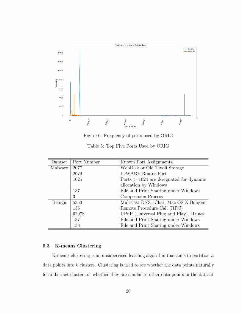
Figure 6: Frequency of ports used by ORIG

Table 5: Top Five Ports Used by ORIG

Dataset Port Number Known Port AssignmentsMalware 2077 WebDisk or Old Tivoli Storage

2079 IDWARE Router Port1025 Ports > 1024 are designated for dynamic

allocation by Windows137 File and Print Sharing under Windows3 Compression Process

Benign 5353 Multicast DNS, iChat, Mac OS X Bonjour135 Remote Procedure Call (RPC)62078 UPnP (Universal Plug and Play), iTunes137 File and Print Sharing under Windows138 File and Print Sharing under Windows

5.3 K-means Clustering

K-means clustering is an unsupervised learning algorithm that aims to partition n

data points into k clusters. Clustering is used to see whether the data points naturally

form distinct clusters or whether they are similar to other data points in the dataset.

20

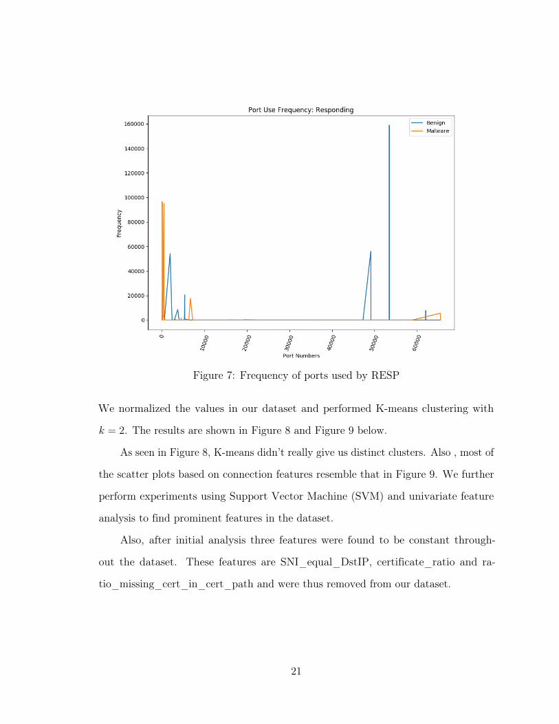
Figure 7: Frequency of ports used by RESP

We normalized the values in our dataset and performed K-means clustering with

k = 2. The results are shown in Figure 8 and Figure 9 below.

As seen in Figure 8, K-means didn’t really give us distinct clusters. Also , most of

the scatter plots based on connection features resemble that in Figure 9. We further

perform experiments using Support Vector Machine (SVM) and univariate feature

analysis to find prominent features in the dataset.

Also, after initial analysis three features were found to be constant through-

out the dataset. These features are SNI_equal_DstIP, certificate_ratio and ra-

tio_missing_cert_in_cert_path and were thus removed from our dataset.

21

Table 6: Top Five Ports Used by RESP

Dataset Port Number Known Port AssignmentsMalware 25 SMTP (Simple Mail Transfer Protocol)

443 HTTPS / SSL - encrypted web traffic53 DNS (Domain Name Service)80 Hyper Text Transfer Protocol (HTTP)6667 IRC (Internet Relay Chat)

Benign 53508 Xsan Filesystem Apple49153 ANTLR, ANother Tool for Language

Recognition1900 IANA registered by Microsoft for SSDP

(Simple Service Discovery Protocol)53 DNS (Domain Name Service)5355 Link-Local Multicast Name Resolution

Windows

22

Figure 8: Original Scatter Plot vs K-means clustering

Figure 9: Original Scatter Plots with different axes

23

5.4 Experiments

This section states multiple experiments conducted using various machine learning

techniques and discusses the results.

5.4.1 SVM with 10-fold cross validation

In this experiment we ran SVM with linear kernel and 10-fold cross validation on

our dataset and achieved an average accuracy rate of 92.06% as shown in Figure 10.

Figure 10: SVM with 10-fold cross-validation

SVM also assigns weights to the input features which provided an insight into the

features SVM believes are important. In Figure 11, we can see that SVM assigned the

highest weight to feature number 16 which is the average certificate length. Table 7

provides us the rank assigned to each feature by SVM. We can see that average

certificate length, periodicity and average public key length are the top most features.

Also from [29] we know that malware use weak encryption techniques such as shorter

key lengths and are more periodic in nature than other applications. Also, the validity

of certificate during capture is the sixth highest rank feature which tell us that most

24

of malware may not have a valid certificate.

Figure 11: Weights assigned to features by SVM

5.4.2 SVM with different kernels

In this experiment SVM was trained on the dataset using different kernels such

as radial basis function (RBF) and polynomial kernel. The 10-fold cross validation

accuracy achieved using different kernels is shown in Figure 12. We can see that all

the kernels give us similar accuracy to that of the linear kernel.

5.4.3 Univariate Feature Elimination

After getting the feature ranks from SVM, we also performed univariate feature

elimination (UFE) to see if the feature ranks provided by SVM matches that of UFE.

We ran UFE with 10-fold cross-validation and plot the ranks along with SVM ranks.

25

Table 7: Top 20 Feature ranks by SVM

Rank Feature1 average_of_certificate_length2 periodicity_standard_deviation3 periodicity_average4 standart_deviation_cert_length5 average_public_key6 is_valid_certificate_during_capture7 average_of_duration8 standard_deviation_duration9 self_signed_ratio10 SNI_ssl_ratio11 ratio_of_differ_sandns_in_cert12 percent_of_established_states13 number_of_certificate_path14 ratio_of_differ_subject_in_cert15 ratio_of_differ_subject_in_ssl_log16 tls_version_ratio17 is_SNI_in_top_level_domain18 total_size_of_flows_orig19 ratio_of_sizes20 ratio_of_differ_issuer_in_ssl_log

As seen in Figure 13, the weight rankings of UFE is almost similar to that of SVM.

5.4.4 SVM with Recursive Feature Elimination

After confirming the SVM feature ranks with that of UFE, we used Recursive

Feature Elimination (RFE) with SVM and 10-fold cross-validation to remove weak

features and calculate the accuracy. RFE iteratively eliminates one feature at a time

and calculates the accuracy until just one feature remains.

As we can see from Figure 14, we get within a 2% of the best result with just 6

features and within 1% with 10 features out of 41. It shows that the top 6 features in

Table 5 contribute the most to the accuracy of the model.

26

Figure 12: SVM with different kernels

5.4.5 Random Forest

In this experiment we ran Random Forest Classifier with Recursive Feature

Elimination and 10-fold cross-validation on the dataset to support the results given

by SVM in previous section. We also ran Random Forest Classifier with different

number of estimators to find the minimum number of estimators required to achieve

a higher accuracy.

The first observation from Figure 15 is that Random Forest gives us a much

higher accuracy than SVM. Also from Figure 16, we can see that the top 5 features

from Random Forest is not the same as SVM. This is because the Random Forest

uses an ensemble of trees where each tree is built using a random selection of features

and the nodes of each tree in the forest is built by selecting and splitting the node to

27

Figure 13: Weights assigned to the features by SVM and UFE

achieve lowest variance [32]. This method of fitting the model on the dataset is very

different as compared to that of SVM.

Figure 17 shows that the accuracy increases when the number of estimators are

increased from 1 to 50 but becomes constant after that and remains the same even

after adding a total of 1000 estimators to the model.

5.4.6 XGBoost

In this experiment we ran XGBoost with Recursive Feature Elimination and

10-fold cross-validation. We also ran XGBoost with different number of estimators to

find the minimum number of estimators required to achieve the highest accuracy.

Figure 18 gives us a similar plot as compared to both SVM and Random Forest

which confirms that accuracy achieved using only the top ten features is almost equal

to the highest accuracy. From Figure 19, we can see that the top 10 features ranked

28

Figure 14: Recursive Feature Elimination with SVM

by XGBoost is different from both Random Forest and SVM. This is because in

boosting the learning is done in a serial way and the feature importance is measured

by number of times a feature is used to split the data across trees.

Also from Figure 17, we can see that the accuracy increases as the number of

estimators are increased from 1 to 1000. The accuracy then remains constant for more

than 1000 estimators. It also shows that we can achieve an accuracy of more than

93%, which is within 7% of the highest accuracy, using only one estimator.

We can also see that XGBoost gives us the highest accuracy of 99.15% followed by

Random Forest which gives us an accuracy of 98.78. Thus, we can say that ensemble

techniques such as XGBoost and Random Forest performs the best on the given

dataset and can be used to identify malicious encrypted traffic.

29

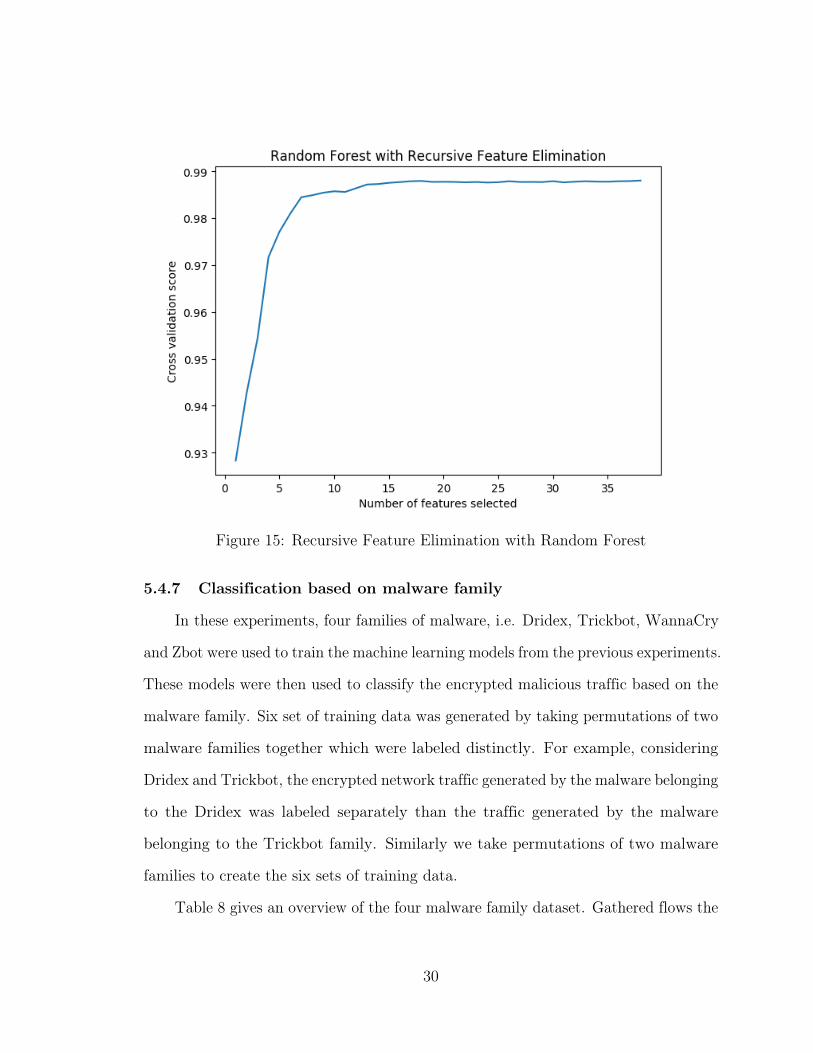
Figure 15: Recursive Feature Elimination with Random Forest

5.4.7 Classification based on malware family

In these experiments, four families of malware, i.e. Dridex, Trickbot, WannaCry

and Zbot were used to train the machine learning models from the previous experiments.

These models were then used to classify the encrypted malicious traffic based on the

malware family. Six set of training data was generated by taking permutations of two

malware families together which were labeled distinctly. For example, considering

Dridex and Trickbot, the encrypted network traffic generated by the malware belonging

to the Dridex was labeled separately than the traffic generated by the malware

belonging to the Trickbot family. Similarly we take permutations of two malware

families to create the six sets of training data.

Table 8 gives an overview of the four malware family dataset. Gathered flows the

30

Figure 16: Random Forest feature importance

are number of connections made whereas the connection 4-tuples is the aggregated

form of the flows where every connection with same source and destination IP, port

and protocol are grouped together as mentioned in Chapter 3.

31

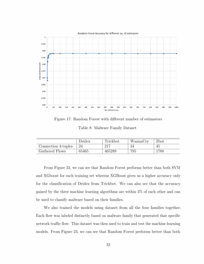
Figure 17: Random Forest with different number of estimators

Table 8: Malware Family Dataset

Dridex Trickbot WannaCry ZbotConnection 4-tuples 24 217 34 45Gathered Flows 65465 465289 785 1788

From Figure 22, we can see that Random Forest performs better than both SVM

and XGboost for each training set whereas XGBoost gives us a higher accuracy only

for the classification of Dridex from Trickbot. We can also see that the accuracy

gained by the three machine learning algorithms are within 3% of each other and can

be used to classify malware based on their families.

We also trained the models using dataset from all the four families together.

Each flow was labeled distinctly based on malware family that generated that specific

network traffic flow. This dataset was then used to train and test the machine learning

models. From Figure 23, we can see that Random Forest performs better than both

32

Figure 18: XGBoost with Recursive Feature Elimination

SVM and XGBoost as seen in earlier experiments. We can also see from previous

experiments that SVM and Random Forest perform better in multi-class classification

problem as compared to when they were used to classify malicious traffic from benign.

33

Figure 19: XGBoost feature importance

5.5 Discussion

As seen in Figure 24, XGBoost performs better than other algorithms. We get an

area under the curve (AUC) value of 0.9988 for XGBoost, whereas SVM and Random

Forest achieve an AUC of 0.9122 and 0.998 respectively. Thus the highest accuracy

gained in our approach is 99.88% which is the same as that achieved by Anderson

34

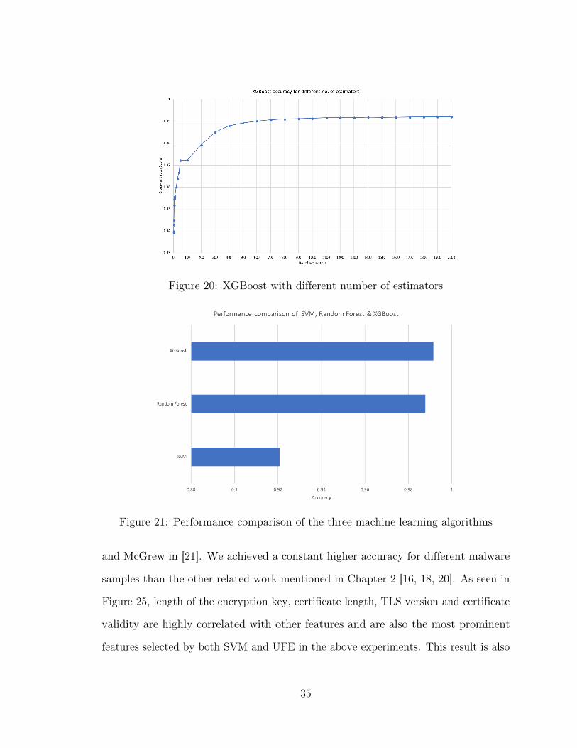
Figure 20: XGBoost with different number of estimators

Figure 21: Performance comparison of the three machine learning algorithms

and McGrew in [21]. We achieved a constant higher accuracy for different malware

samples than the other related work mentioned in Chapter 2 [16, 18, 20]. As seen in

Figure 25, length of the encryption key, certificate length, TLS version and certificate

validity are highly correlated with other features and are also the most prominent

features selected by both SVM and UFE in the above experiments. This result is also

35

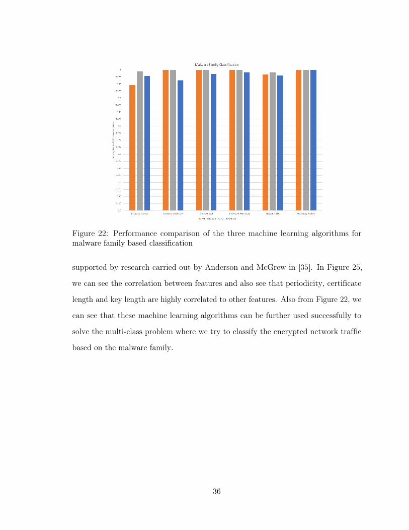
Figure 22: Performance comparison of the three machine learning algorithms formalware family based classification

supported by research carried out by Anderson and McGrew in [35]. In Figure 25,

we can see the correlation between features and also see that periodicity, certificate

length and key length are highly correlated to other features. Also from Figure 22, we

can see that these machine learning algorithms can be further used successfully to

solve the multi-class problem where we try to classify the encrypted network traffic

based on the malware family.

36

Figure 23: Performance comparison of the three machine learning algorithms formulti-class problem

Figure 24: Comparison of various machine learning algorithms

37

Figure 25: Feature correlation heat map

38

CHAPTER 6

Conclusion and Future Work6.1 Conclusion

With an increase in worldwide adoption of HTTPS and advancement in malware

detection techniques, we will see an increase in the number of malware samples

using HTTPS and encryption to evade detection and hide their malicious activity. It

is worrying because encryption interferes with the traditional detection techniques.

Identifying such threats in a way that is feasible, fast and does not compromise user

security is an important problem. Machine learning methods have been proven to

overcome traditional limitations and can be used to train models on malware network

traffic data. These models can then be used to detect similar malicious network traffic

and flag a system for malware infection. Further, the system can be isolated to prevent

further propagation of malware on the internal network.

The primary motivation of this research is the challenging problem of classifying

encrypted network traffic as malicious or benign without using any decryption or deep

packet inspection. In this research, we used several machine learning algorithms such

as SVM, XGBoost, random forest to classify malicious and non-malicious encrypted

network traffic. These algorithms were used to train and test models which can be

used for classification. The results show that XGBoost performed better than other

algorithms and reached the highest accuracy of 99.15%. We also achieved a high

accuracy using only top six or top 10 features from Table 7. The results also support

that machine learning models can be used to solve the multi-class problem. Thus,

we can conclude that encrypted malware network traffic is distinct from the normal

traffic and it also differ from one malware family to another. This property can be

used to successfully identify an infected host and also specify the malware family with

which the host was infected.

39

6.2 Future Work

There is a lot of scope to further improve the accuracy in future work. The

next step would be to collect more data for training and testing the models and find

additional features that could be useful in classification. Obtaining public network

captures is harder due to the privacy issues involved. Thus, future work might include

setting up a lab to generate both malicious as well as non-malicious network captures.

The malicious network captures can be generated by running the latest malware

samples that are uploaded to VirusTotal [36] in a virtual environment and recording

the network traffic. Another step in data collection would be to collect more data

from malware samples belonging to the same malware family. An interesting direction

might be to try tools other than Bro to extract novel features and use them to try

additional machine learning algorithms. Lastly, the future work might also include

deploying the model on a real-world network to test the performance and robustness

of the proposed approach.

40

LIST OF REFERENCES

[1] J. Aycock, Computer Viruses and Malware, ser. Advances in Information Security.Springer, 2006, vol. 22.

[2] Malwarebytes, ‘‘Analysis of malware trends for small and mediumbusinesses, Q1-2017,’’ https://www.malwarebytes.com/pdf/white-papers/MalwareTrendsForSMBQ12017.pdf, March 2017.

[3] S. Sen, O. Spatscheck, and D. Wang, ‘‘Accurate, scalable in-network identifi-cation of p2p traffic using application signatures,’’ in Proceedings of the 13thinternational conference on World Wide Web, ser. WWW 2004, S. I. Feldman,M. Uretsky, M. Najork, and C. E. Wills, Eds. ACM, 2004, pp. 512--521.

[4] Google, ‘‘Https encryption on the web,’’ https://transparencyreport.google.com/https/, March 2017.

[5] B. Anderson, ‘‘Hiding in plain sight: Malware’s use of TLS and encryption,’’ https://blogs.cisco.com/security/malwares-use-of-tls-and-encryption, CISCO Blogs,2016.

[6] Radware, ‘‘Global application and network security report 2016-17,’’ https://www.radware.com/PleaseRegister.aspx?returnUrl=644245912, 2017.

[7] S. Yoon, J. Park, J. Park, Y. Oh, and M. Kim, ‘‘Internet application trafficclassification using fixed ip-port,’’ in Proceedings of Management Enabling theFuture Internet for Changing Business and New Computing Services, 12th Asia-Pacific Network Operations and Management Symposium, ser. APNOMS 2009,C. S. Hong, T. Tonouchi, Y. Ma, and C. Chao, Eds. Springer, 2009, pp. 21--30.

[8] ‘‘IANA: Service name and transport protocol port number registry,’’ http://www.iana.org/assignments/port-numbers.

[9] H. Dreger and A. Feldmann, ‘‘Dynamic application-layer protocol analysis fornetwork intrusion detection,’’ in Proceedings of the 15th USENIX Security Sym-posium, ser. USENIX Security ’15, A. D. Keromytis, Ed. USENIX Association,2006.

[10] S. Baset and H. Schulzrinne, ‘‘An analysis of the Skype peer-to-peer internettelephony protocol,’’ in 25th IEEE International Conference on Computer Com-munications, ser. INFOCOM 2006. IEEE, 2006.

41

[11] A. Madhukar and C. L. Williamson, ‘‘A longitudinal study of P2P traffic classifi-cation,’’ in 14th International Symposium on Modeling, Analysis, and Simulationof Computer and Telecommunication Systems, ser. MASCOTS 2006. IEEEComputer Society, 2006, pp. 179--188.

[12] L. Etienne, ‘‘Malicious traffic detection in local networks with snort,’’ https://infoscience.epfl.ch/record/141022/files/pdm.pdf, 2009.

[13] Snort, ‘‘Snort --- Network intrusion detection and prevention system,’’ https://www.snort.org.

[14] ‘‘Snort: Community rules,’’ https://www.snort.org/downloads/community/community-rules.tar.gz, 2016.

[15] A. W. Moore and K. Papagiannaki, ‘‘Toward the accurate identification ofnetwork applications,’’ in Proceedings of 6th International Workshop on Passiveand Active Network Measurement, ser. PAM 2005, C. Dovrolis, Ed. Springer,2005, pp. 41--54.

[16] F. Tegeler, X. Fu, G. Vigna, and C. Kruegel, ‘‘Botfinder: finding bots in networktraffic without deep packet inspection,’’ in Conference on emerging NetworkingExperiments and Technologies, ser. CoNEXT ’12, C. Barakat, R. Teixeira, K. K.Ramakrishnan, and P. Thiran, Eds. ACM, 2012, pp. 349--360.

[17] X. Wang, W. Qiu, and R. H. Zamar, ‘‘CLUES: A non-parametric clusteringmethod based on local shrinking,’’ Computational Statistics & Data Analysis,vol. 52, no. 1, pp. 286--298, 2007.

[18] P. Prasse, L. Machlica, T. Pevný, J. Havelka, and T. Scheffer, ‘‘Malware detectionby analysing network traffic with neural networks,’’ in 2017 IEEE Security andPrivacy Workshops, ser. SPW 2017, 2017, pp. 205--210.

[19] Z. Hu, L. Zhu, J. Heidemann, A. Mankin, D. Wessels, and P. Hoffman, ‘‘RFC7858: Specification for DNS over Transport Layer Security (TLS),’’ http://www.isi.edu/%7ejohnh/PAPERS/Hu16a.html, 2016.

[20] J. Lokoc, J. Kohout, P. Cech, T. Skopal, and T. Pevný, ‘‘k-nn classification ofmalware in HTTPS traffic using the metric space approach,’’ in Proceedings ofIntelligence and Security Informatics, ser. PAISI 2016, M. Chau, G. A. Wang,and H. Chen, Eds. Springer, 2016, pp. 131--145.

[21] B. Anderson and D. A. McGrew, ‘‘Machine learning for encrypted malware trafficclassification: Accounting for noisy labels and non-stationarity,’’ in Proceedingsof the 23rd ACM International Conference on Knowledge Discovery and DataMining, ser. SIGKDD 2017. ACM, 2017, pp. 1723--1732.

42

[22] R. Sommer and V. Paxson, ‘‘Outside the closed world: On using machinelearning for network intrusion detection,’’ in 31st IEEE Symposium on Securityand Privacy, ser. S&P 2010. IEEE Computer Society, 2010, pp. 305--316.

[23] T. Hastie, R. Tibshirani, and J. H. Friedman, The Elements of Statistical Learn-ing: Data Mining, Inference, and Prediction, 2nd ed., ser. Springer series instatistics. Springer, 2009.

[24] S. García, M. Grill, J. Stiborek, and A. Zunino, ‘‘An empirical comparison ofbotnet detection methods,’’ Computers & Security, vol. 45, pp. 100--123, 2014.

[25] M. J. Erquiaga and S. Garcia, ‘‘Malware capture facility project,’’ https://mcfp.weebly.com, CVUT University, 2013.

[26] ‘‘Bro network security monitor,’’ https://www.bro.org.

[27] A. O. Freier, P. Karlton, and P. C. Kocher, ‘‘RFC 6101: The secure sockets layer(SSL) protocol version 3.0,’’ 2011.

[28] F. Strasak, ‘‘Detection of HTTPS malware traffic, Thesis, Czech TechnicalUniversity,’’ https://dspace.cvut.cz/bitstream/handle/10467/68528/F3-BP-2017-Strasak-Frantisek-strasak_thesis_2017.pdf.

[29] B. Anderson and D. A. McGrew, ‘‘Identifying encrypted malware traffic withcontextual flow data,’’ in Proceedings of the 2016 ACM Workshop on ArtificialIntelligence and Security, ser. AISec@CCS 2016, D. M. Freeman, A. Mitrokotsa,and A. Sinha, Eds. ACM, 2016, pp. 35--46.

[30] M. Stamp, Introduction to Machine Learning with Applications in InformationSecurity. Boca Raton: Chapman and Hall/CRC, 2017.

[31] T. K. Ho, ‘‘Random decision forests,’’ in Third International Conference onDocument Analysis and Recognition, ser. ICDAR 1995. IEEE Computer Society,1995, pp. 278--282.

[32] B. Holczer, ‘‘Random forest classifier machine learning,’’ http://www.globalsoftwaresupport.com/random-forest-classifier-bagging-machine-learning/.

[33] T. Chen and C. Guestrin, ‘‘XGBoost: A scalable tree boosting system,’’ http://arxiv.org/abs/1603.02754.

[34] J. Brownlee, ‘‘A gentle introduction to XGBoost for applied machine learn-ing,’’ https://machinelearningmastery.com/gentle-introduction-xgboost-applied-machine-learning/.

[35] B. Anderson, S. Paul, and D. A. McGrew, ‘‘Deciphering malware’s use of TLS(without decryption),’’ https://arxiv.org/pdf/1607.01639.pdf, 2016.

43

[36] ‘‘VirusTotal --- Free online virus, malware and URL scanner,’’ https://www.virustotal.com.

44