Analysis of Electromagnetic and Seismic Geophysical Methods for

Investigating Shallow Sub-surface Hydrogeology

Eric M. Parks

A thesis submitted to the faculty of

Brigham Young University

in partial fulfillment of the requirements for the degree of

Masters of Science

Stephen T. Nelson, Chair

John H. McBride

Alan L. Mayo

Department of Geological Sciences

Brigham Young University

April 2010

Copyright © 2010 Eric M. Parks

All Rights Reserved

ABSTRACT

Analysis of Electromagnetic and Seismic Geophysical Methods for

Investigating Shallow Sub-surface Hydrogeology

Eric M. Parks

Department of Geological Sciences

Master of Science

An integrated electromagnetic (EM) and seismic geophysical study was performed to evaluate non-invasive approaches to estimate depth to shallow groundwater in arid environments with elevated soil salinity where the installation of piezometers would be impractical or prohibited. Both methods were tested in two study areas (semi-arid and arid respectively), one in Palmyra, Utah, USA near the shore of Utah Lake where groundwater is shallow and unconfined in relatively homogeneous lacustrine sediments. The other area is Carson Slough, Nevada, USA near Ash Meadows National Wildlife Refuge in Amargosa Valley. The area is underlain by valley fill, with generally variable shallow depths to water in an ephemeral braided stream environment. The methods used include frequency domain electromagnetic induction allowing for multiple antenna-receiver spacings. High resolution compressional P-wave seismic profiles using a short (0.305 m) geophone spacing for common depth-point reflection stacking and first arrival modeling were also acquired. Both methods were deployed over several profiles where shallow piezometer control was present. The semi-arid Palmyra site with its simpler geohydrology serves as an independent calibration to be compared to the Carson Slough Site.

EM results at both sites show that water surfaces correspond with a drop in conductivity. This is due to elevated concentrations of evaporative salts in the vadose zone immediately above the water table. EM and seismic profiles at the Palmyra site were readily correlated to depth to groundwater in monitoring wells demonstrating that the method is ideal under laterally homogeneous conditions. Interpreting the EM and seismic profiles at Carson Slough was challenging due to the laterally and vertically variable soil types, segmented perched water surfaces, and strong salinity variations.

The high-resolution images and models provided by the seismic profiles confirm the simple soil and hydrological structure at the Palmyra site as well as the laterally complex structure at Carson Slough. The EM and seismic results indicate that an integrated geophysical approach is necessary for an area like Carson Slough, where continued leaching of salts combined with braided stream deposition has created a geophysically complex soil and groundwater system.

ACKNOWELDGEMENTS

There are many people that I have reason to be grateful to for helping me reach my goal

of graduating with a master’s degree. I cannot name them all here, but I would first like to thank

Dr. Steve Nelson, Dr. John McBride, Dr. Alan Mayo, and Prof. David Tingey for their help from

the beginning stages of this thesis project. Thank you each for always being available to help me

with my questions, both in coursework and my thesis research. I would also like to thank all the

professors and student assistants who helped me with field work in summer heat of the

Amargosa Desert and along the shore of Utah Lake.

I gratefully acknowledge software grants to Brigham Young University from the

Landmark (Halliburton) University Grant Program (ProMAX2D™) and from Seismic Micro-

Technology (The Kingdom Suite™). Partial funding for this project was provided by Nye

County (Nevada) Department of Natural Resources and by the College of Physical and

Mathematical Sciences, Brigham Young University. I would also like to thank the Nature

Conservancy for allowing me allowing me to use their property in Palmyra, Utah for a portion of

this study.

Lastly I would like to thank my family for their support. I would like to thank my parents

who have always encouraged me to explore, to learn, and to reach for my goals. Finally, I want

to thank my wife Sarah for her support all along my journey as a graduate student. She has

helped me in the field, in the lab, at home, and at conferences.

iv

TABLE OF CONTENTS INTRODUCTION ...........................................................................................................................1

Study Areas ................................................................................................................................. 2

Local Geologic and Hydrogeologic Settings .............................................................................. 3

Purpose and Objectives ............................................................................................................... 4

Previous Studies and Significance of Project ............................................................................. 5

METHODS ......................................................................................................................................7

Transect Locations ...................................................................................................................... 7

Soil Analyses .............................................................................................................................. 7

EM Conductivity Soundings ....................................................................................................... 8

Seismic Reflection and Refraction .............................................................................................. 9

RESULTS ......................................................................................................................................11

Palmyra Site .............................................................................................................................. 11

Soil and Water....................................................................................................................... 11

EM Model Results ................................................................................................................ 11

Seismic Results ..................................................................................................................... 12

Carson Slough Site .................................................................................................................... 13

Soil and Water....................................................................................................................... 13

EM Model Results ................................................................................................................ 14

Seismic Results ..................................................................................................................... 14

DISCUSSION ................................................................................................................................16

CONCLUSIONS............................................................................................................................21

REFERENCES ..............................................................................................................................24

FIGURES .......................................................................................................................................29

TABLES ........................................................................................................................................43

APPENDIX A ................................................................................................................................48

v

LIST OF TABLES

Table 1. AA Na+ ion data .......................................................................................................... 43

Table 2. USCS soil symbols for all augered holes.................................................................... 44

Table 3. Well data for all Carson Slough and Palmyra wells ................................................... 47

LIST OF FIGURES Figure 1. Index map .................................................................................................................. 29

Figure 2. Cross section of Palmyra, UT site ............................................................................. 30

Figure 3. Direct measurements of soil conductivity for Palmyra, UT site ............................... 31

Figure 4. Na+ ion concentration from leachate for Palmyra, UT well 1 ................................... 32

Figure 5. FEM models for Palmyra, UT site ............................................................................ 33

Figure 6. Seismic profile for Palmyra, UT site ......................................................................... 34

Figure 7. Locations of wells 1-9 and profiles 1-4 for Carson Slough, NV site ........................ 35 Figure 8. Cross section for line 2 at Carson Slough ................................................................. 36

Figure 9. Direct measurements of soil conductivity for wells 4 and 5 at Carson Slough ......... 37

Figure 10. FEM profile for line 1 at Carson Slough ................................................................. 38

Figure 11. FEM models and profile for line 2 at Carson Slough ............................................ 399

Figure 12. Seismic profile for line 1 at Carson Slough............................................................. 40

Figure 13. Seismic profile for line 2 at Carson Slough............................................................. 41

Figure 14. Conceptualized model of subsurface at Carson Slough .......................................... 42

Figure 15. Interpretation of depth to water from FEM models for line 2 at Carson Slough .... 42

1

INTRODUCTION

Characterization of water resources in arid environments that face human development is

critical. Desert regions often have abundant biological diversity, as well as many endangered or

threatened species, which depend on these shallow water systems. The Amargosa Desert is one

of the driest regions in the western USA and several species there are facing pressure from

modern human development and urban expansion (Anderson, 2005; Hasselquist and Allen,

2009; Johnston and Zink, 2003; Sada, 1990). Better constraints on understanding shallow (<5

m) groundwater in this type of region could be determined by drilling or trenching; however, this

is often impractical, prohibitively expensive, or, in protected habitats, generally prohibited. For

these reasons, there are many desert areas where a non-invasive approach to mapping shallow

groundwater could be very valuable. Geophysical tools may be of use to provide the needed data

to estimate depth to water. However, the use of classical geophysical methods (e.g., seismic

refraction and electrical resistivity) to measure depth to shallow ground water (< 5 m) in areas

with high soil and water salinity and complex shallow geology presents many challenges. This

study is meant to determine the effectiveness and feasibility of frequency domain

electromagnetic (FEM) conductivity measurements and shallow high-resolution seismic methods

to determine depth to and lateral structure of shallow groundwater in arid regions with elevated

soil salinity, and complex near-surface geology. Seismic profiles were collected to provide a

calibration and comparison to FEM measurements.

Understanding depth to shallow groundwater in arid regions is critical for accurate

estimation of water loss due to evapotranspiration (ET). Carson Slough is one such area where

water resources are facing increased pressure by human development. Its location, adjacent to

Ash Meadows Wildlife Refuge, with several endangered species of plants and animals (Sada,

2

1990), and proximity to growing cities like Pahrump, Nevada, which has shown continued

population growth and a net decrease in water levels of up to 18.3 m in the valley fill aquifer due

to pumping (Harrill, 1986; Stonestrom et al., 2007), makes it a good location for this geophysical

study. Greater accuracy in depth to water estimates could contribute to better ET estimates

which will improve the water budget resulting in more sustainable use of water in the area.

Study Areas

In order to provide a simple control on the interpretation of geophysical data from the

arid site, two study areas were selected. The first is 450 m from the southern shore of Utah Lake,

in Palmyra, Utah near the Provo Bay outlet (Figure 1-A). The second is at Carson Slough,

Nevada south of Ash Meadows National Wildlife Reserve (AMNWR) in the Amargosa Desert

located about 115 km northwest of Las Vegas, Nevada (Figure 1-B). The majority of soil

samples from both study areas indicate that the soils would be classified as saline soils, defined

by an electrical conductivity (EC) of the saturation extract >4 dS/m (400mS/m), although many

scientists are urging that the minimum EC for saline soils be defined as >2dS/m (400 mS/m)

(Rhoades, 1993; Sparks, 2003).

The Utah Lake site was chosen because it is similar to Carson Slough in being semi-arid

and with elevated salinity and shallow water, but less sedimentologically and hydrogeologically

complex, allowing for comparison of the data and evaluation of the methodology in two different

ranges of complexity.

The site at Carson Slough was chosen for its proximity to AMNWR, a protected area

where water levels are shallow, not well defined, and a non-invasive approach to determine

depth to groundwater would be greatly beneficial.

3

Local Geologic and Hydrogeologic Settings

The Palmyra site is located in southern Utah Valley, which is part of the Utah Lake

watershed of the Great Salt Lake Basin (Figure 1). Utah Valley formed as a result of Tertiary

Basin and Range extension and corresponds to the boundary between the Basin and Range and

Rocky Mountain Provinces (Clark and Apple, 1985). The shallow valley subsurface is

composed mainly of Quaternary fluvial sediments and Pleistocene Lake Bonneville sediments

and inter-fingered alluvial fan deposits (Bissel, 1963; Sanderson, 2002). Surface sediments at

the Palmyra site have been mapped as sand and silty alluvium, upper Pleistocene to Holocene in

age (Bissel, 1963).

Four significant groundwater systems have been identified within Utah Valley and the

bounding Wasatch mountains, (Barnhurst, 2003); however, only the upper portion of the shallow

alluvial groundwater system is of interest to this particular investigation. Sediments in this

generally unconfined aquifer are granular sediments with only sparse and thin confining units

(Utah Division of Water Resources, 1997). Water levels in this area range from about 1.5 m

below ground surface near the lake to about 120 m near the Wasatch Mountain front to the east

(Sanderson, 2002). Because the location of investigation is so close to the lake, the water table

varies only with fluctuations in lake level. The average precipitation for the area is 52.5 cm/yr

(Sanderson, 2002).

The Carson Slough site is located in the Amargosa Desert, which is part of the Death

Valley watershed in southwestern Nevada and southeastern California (Figure 1). It has a

surface drainage area of about 6700 km2 (Walker and Eakin, 1963) and ranges in elevation from

670 m to 2100 m with corresponding mean annual precipitation ranging from 5 cm to 38 cm

(Classen, 1985). The Amargosa basin is bounded by northwest-trending mountain ranges of

4

Precambrian quartzite and Paleozoic quartzite and dolomite (Sweetkind et al., 2001). The basin

formed as a result of middle to late Cenozoic Basin and Range extension (Grose and Smith,

1989). Valley fill, which reaches thicknesses of up to 550 m (Winograd and Thordarson, 1975),

is composed of alluvial fans, playas, eolian, lacustrine, fluvial, and spring deposits (Workman et

al., 2001). Kilroy (1991) classified and described the valley fill sediments into five lithologies as

follows: moderately sorted river-channel sediments from clay to gravel size, poorly to well-

sorted, fine-grained playa sediments, poorly-sorted silt to gravel sized alluvial fan sediments,

fine-grained vuggy freshwater limestones, and moderately indurated Tertiary conglomerates.

Winograd and Thordarson (1975) remarked that the valley fill is generally poorly stratified and

poorly sorted and that strata are horizontal but usually discontinuous. They also noted that

caliche is a cementing agent found at almost all depths. The valley fill is underlain by lava

flows, tuffs, and Paleozoic carbonates, sandstones, mudstones, and conglomerates (Workman et

al., 2001).

Four main hydrogeologic units exist in the Amargosa Basin. These have been identified

by Winograd and Thordarson (1975) as the valley-fill, tuff, and upper and lower carbonate

aquifers; however, only the shallow groundwater found in the valley fill is of interest to this

study. Quittmeyer, (2000) also noted occurrences of perched water in the Amargosa region

within the valley fill.

Purpose and Objectives

The purpose of this study is to evaluate the effectiveness and feasibility of frequency

electromagnetic (FEM) conductivity soundings and shallow seismic reflection to measure depth

to shallow water and its vertical and lateral variability in arid environments with elevated soil

salinity. The objectives are first to determine how FEM conductivity data can be modeled to

5

create a depth profile that sufficiently correlates with the actual conductivity profile; second, to

determine how conductivity profiles can be interpreted to correspond with shallow water

surfaces in arid regions with elevated salinity; third, to determine how shallow high-resolution

seismic reflection can be used in combination with EM models to improve interpretations of EM

conductivity models of the shallow water table, and; fourth, to evaluate these methods’

effectiveness and feasibility for use on larger scale hydrogeological investigations such as

evapotranspiration estimates.

Previous Studies and Significance of Project

Numerous studies on the hydrogeology of the Amargosa Desert have been completed as

early as the 1950’s (Anderson, 2002; Kilroy, 1991; Classen, 1985; Grose and Smith, 1989;

Kilroy, 1991; Laczniak et al., 1999; Walker and Eakin, 1963; Winograd and Thordarson, 1975;

and references therein). Despite the importance of the shallow valley-fill aquifer, which serves

as the main water supply for the Amargosa Desert, there are inconsistencies in reports of depth to

water within it. Measurements at Carson Slough, directly adjacent to AMNWR, range from 1 to

10 m (Anderson, 2002; Kilroy, 1991; Laczniak et al., 1999; Walker and Eakin, 1963; Winograd

and Thordarson, 1975).

Geophysical methods have been used for many years to solve hydrogeological problems

(Kelly, et al. 1993; Reynolds, 1997); however, very little has been done to examine the ability of

loop-loop frequency domain EM and seismic to measure depth to groundwater in shallow saline

conditions.

EM instrumentation has been used in numerous hydrogeological studies, but typical

applications differ from those of this study. There are a variety of EM instruments which are

generally selected on the basis of the desired depth of exploration. Small loop loop FEM

6

instruments are generally the tools of choice for shallow (<10 m) EM exploration (Mitsuhata, et

al., 2006). FEM instruments are typically used in an effort to determine lateral extent of

groundwater (Potts, 1990), mapping groundwater contamination plumes (Al-Tarazi, et al., 2008;

Buselli, et al., 1992), mapping subsurface discontinuities (Potts, 1990; Stroh et al., 2001;

Sengpiel, 1998), measuring near-surface soil moisture (Sheets and Hendrickx, 1995; Persson and

Haridy, 2003), and determining depth to claypan (Brus et al., 1992; Cockx and De Vos, 2007;

Doolittle, et al., 1994). In cases where vertical resolution is needed, such as determining

hydrostratigraphy or detection of salt water interfaces in freshwater aquifers, transient

electromagnetic (TEM) is considered favorable; however, most of these instruments are limited

to deeper targets (Fitterman, and Stewart, 1986). Traditionally, TEM instruments are used to

explore depths >50 m, and interpretation methods are more complex but have been used with

success (Fitterman and Stewart, 1986; Fitterman et al., 1999), although some new nano TEM

instruments are capable of investigations in the upper 1-30 m. The shallow limit of TEM

accuracy is a function of conductivity, and results in variable resolution in the shallow zone

(Urquhart, 2009). The upper 4 m mainly reflects pore fluid salinity (Tan et al., 2007). More

detailed explanation of EM theory and principles of operation are given by Nabighian, and

Corbett (1991).

Integration of seismic and electromagnetic data has been previously applied in the

Amargosa Desert (Louie et al., 1997). Their goal was not for hydrogeological characterization

but a similar combination of methods (FEM, TEM, and seismic) were successfully integrated in

the characterization of the Pahrump Valley fault zone.

Although seismic reflection and refraction have been used many times to measure depth

to water (especially refraction), the seismic method is not typically aimed at imaging ultra-

7

shallow (<3 m) layers. There is no guarantee that a capillary fringe will not prevent a reflection

from being detected (Kelly and Mares, 1993). However, Baker et al. (2000) performed one such

experiment where ultra-shallow seismic reflection was successfully used to measure seasonal

fluctuations in sub-meter depth to groundwater near the Arkansas River in Kansas. Their

accuracy was within 12 cm; however, their geophone spacing was only 2 inches (5 cm), and their

acoustic source was a .22 caliber rifle.

METHODS

Transect Locations

Four 200-m straight-line transects were chosen at the Carson Slough site (Figures

1-B, and 7) so as to correspond to existing piezometers, which served as control points. FEM

and seismic data were collected along each line for comparison. One 100-m straight-line

transect at the Palmyra site (Figure 1-A) was chosen based on the flatness of the ground surface,

the shallow depth to groundwater, and absence of dense vegetation that otherwise covered the

area. In order to provide a control transect in an area similar to the Carson Slough site, but with

a much simpler structure, FEM and seismic data were collected along a profile at the Palmyra

site using the same parameters. Two piezometers were installed near each end of the profile as

control points so the geophysical data could be compared with actual depth to water

measurements.

Soil Analyses

In order to create cross sections of the vadose zone to upper phreatic zone, soil samples

were collected adjacent to piezometer holes at wells 1, 2, and 3 at the Palmyra site and along

wells 2, 4, 5, and 6 at the Carson Slough site. Samples were taken approximately every 1-2 ft

(0.3-0.6 m) for construction of a cross section of the soil profile, and for further analysis

8

including direct conductivity measurements, x-ray diffraction (XRD) analysis, and analysis of

leachate on the flame atomic absorption spectrometer (AA). These data were collected for

comparison with geophysical data. The depths associated with the augered soil samples are

approximate, due to the shape of the auger bucket which collects soil within a 0.3 m long

cylinder with a 0.1 m diameter. Samples were assigned depths corresponding to the middle of

the bucket during sampling. The direct conductivity measurements were taken for comparison to

EM conductivity profiles in order to confirm the instrument readings. This was done using by

making a slurry with 30 g of soil sample and 30 mL of de-ionized water and analyzing it with a

YSI brand salinity-conductivity-temperature gauge. XRD analysis for determining quantitative

mineralogy was done using procedures outlined by Ebel (2003) for powdered samples using a

Scintac Inc XRD and processing the data using the United States Geological Survey (USGS)

program “RockJock” (Eberl, 2003). A Perkin Elmer 1500PC atomic absorption spectrometer

was used to examine concentrations of Na+ ions at various depths along the profile of one well.

This was done by mixing 40 g of soil sample with 80mL de-ionized water and allowing it to

equilibrate, then using the leachates from each sample for analysis (Table 1).

EM Conductivity Soundings

Typically EM hydrogeological studies use a single instrument for data acquisition. For

this study three FEM conductivity meters were chosen to achieve the necessary range of

penetrations to create a depth profile at each sounding. The three FEM instruments used were

the Geonics EM-38 (14.6 kHz with 1-m coil separation), EM-31-SH (9.8 kHz with 2-m coil

separation), and EM-34 (6.4 kHz and 1.6 kHz with 10-m and 20-m coil separations respectively.

They have effective penetrations of 1.5-m, 3-m, 15-m, and 30-m respectively. This array of

instruments allows for 12 conductivity soundings at each point. Measurements with the EM-38

9

and EM31-SH were taken in both horizontal and vertical dipole orientations at the user’s hip

height and at the ground surface. The EM-34 was used in vertical and horizontal orientation at

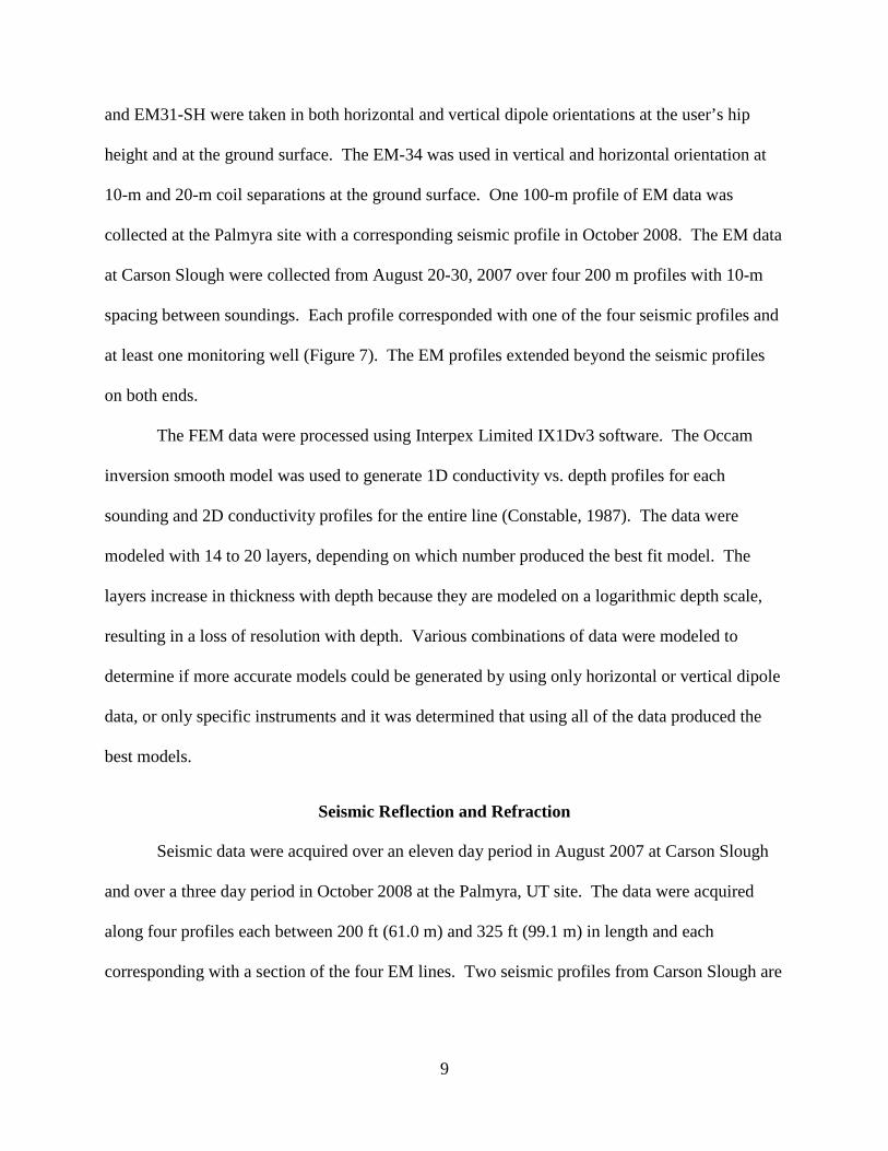
10-m and 20-m coil separations at the ground surface. One 100-m profile of EM data was

collected at the Palmyra site with a corresponding seismic profile in October 2008. The EM data

at Carson Slough were collected from August 20-30, 2007 over four 200 m profiles with 10-m

spacing between soundings. Each profile corresponded with one of the four seismic profiles and

at least one monitoring well (Figure 7). The EM profiles extended beyond the seismic profiles

on both ends.

The FEM data were processed using Interpex Limited IX1Dv3 software. The Occam

inversion smooth model was used to generate 1D conductivity vs. depth profiles for each

sounding and 2D conductivity profiles for the entire line (Constable, 1987). The data were

modeled with 14 to 20 layers, depending on which number produced the best fit model. The

layers increase in thickness with depth because they are modeled on a logarithmic depth scale,

resulting in a loss of resolution with depth. Various combinations of data were modeled to

determine if more accurate models could be generated by using only horizontal or vertical dipole

data, or only specific instruments and it was determined that using all of the data produced the

best models.

Seismic Reflection and Refraction

Seismic data were acquired over an eleven day period in August 2007 at Carson Slough

and over a three day period in October 2008 at the Palmyra, UT site. The data were acquired

along four profiles each between 200 ft (61.0 m) and 325 ft (99.1 m) in length and each

corresponding with a section of the four EM lines. Two seismic profiles from Carson Slough are

10

discussed herein, one representing a typically shallow water level (~ 1 m) and one representing a

typically deep level (~ 3 m) (profiles 1 and 2, respectively).

Seismic acquisition parameters were chosen for high resolution in the shallow subsurface.

These included using a 1-kg mallet source (4.5 kg sledge hammer source when windy conditions

created excessive noise), 96 channel, common depth-point (CDP) recording, 28-Hz vertical

geophones, 0.125 ms sample rate, field filters: 35-Hz (Palmyra) & 200-Hz (Carson Slough) low-

cut, 1 ft (~0.3-m) geophone spacing, and stacking shot records three times to reduce noise.

The data were first converted from SEG-2 to SEG-Y format and assigned 3D geometry.

Records were examined for quality and bad traces were deleted. Appropriate mute functions

were applied to eliminate first arrivals (direct and head waves) to bring out deeper reflections.

The air blast was also muted in order to allow better resolution of very shallow reflections. An

Ormsby bandpass filter (100-200-700-900 Hz (zero phase) for Carson Slough; 100-120-300-700

Hz (minimum phase for Palmyra)) was then applied followed by a deconvolution to compress

the wavelets and reduce multiple reflections. Post-stack was also applied. Automatic gain

control (200-ms window for Carson Slough; 100-ms for Palmyra) was applied, followed by CDP

stacking, velocity analysis and conversion from time to depth. The stacks are displayed with a 5-

trace weighted mix in order to suppress low-apparent velocity noise. Since our targets were very

shallow (< 5 m), depth conversion was applied using a velocity appropriate for the uppermost

soils, based on the direct arrival or the lowest normal move-out (NMO) velocity. Note that no

elevation static correction is applied so as to afford direct comparison with the EM modeling,

which is referenced to the ground surface. Elevation changes along the profiles were relatively

small (usually < 0.5 m). Each CDP section was stacked with an NMO velocity appropriate to the

water level depth expected from the nearest well(s). In addition to processing the seismic data

11

for CDP reflection, classical modeling of the direct arrivals and head waves was also performed

for a two-layer case and the results plotted directly on the CDP stacked sections.

RESULTS

Palmyra Site

Soil and Water

The soil profiles from all three augered holes have an identical progression of soil types

(Figure 2). The upper 2.1 m is silt with a silty sand layer from approximately 2.1 to 2.4 m

followed by silt increasing in moisture content until saturation. Water levels were 9.5 ft (2.9 m)

in well 1 and 9.8 ft (3 m) in well 2 (Table 3). Samples from wells 1 and 2 were used to make a

slurry from which direct measurements of conductivity were taken for comparison to EM

conductivity profiles (Figure 3). Samples from Palmyra well 1 and Carson Slough well 4 were

also analyzed by XRD to determine mineralogy and attempt to quantify salts; however, salinity

concentrations were too low to quantify accurately. The approximate mineralogy, determined by

XRD analysis, can be found in Appendix A-1 and A-2. Major minerals include quartz, Na-

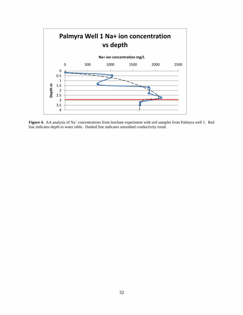
smectite, calcite, dolomite, and anorthoclase feldspar. Results from AA analysis of leachate

from Palmyra well 1 samples show Na+ concentrations generally increasing with depth and

decreasing at or just above the water table (Figure 4). These soil analyses were useful in

comparison and confirmation of geophysical data as well as confirming the link between salinity

and conductivity trends.

EM Model Results

Modeling of FEM data was performed along the line indicated in Figure 1-A. Results

show that the conductivity vs. depth profile of the first nine stations along the line were similar

12

both in conductivity magnitudes and pattern over depth in the upper 6 m while results for station

10 (located on a compacted dirt road) were less similar outside of the 2-6 m range. The overall

trend in conductivity shows a gradual increase with increasing depth up to approximately 3 m.

At 3 m conductivity drops and remains relatively consistent to the bottom of the profile at 30 m

(Figure 5), although, less confidence is put in these data past a depth of 6 m due to a decrease in

resolution with depth and interference with higher conductivity of the shallower zones. Raw

data can be examined in Appendix A-3. Overall, the EM data quality for the Palmyra site was

high quality and provided a good calibration for EM analysis and modeling at Carson Slough.

Modeled EM values range from 10-20 mS/m at the surface, to 100-150 mS/m in the mid-vadose

zone, to ~1000 mS/m at the peak above the vadose-phreatic boundary.

Seismic Results

One seismic survey was performed at the Palmyra site (Figure 6) located along the same

line as the EM profile (Figure 1-B) and extended for approximately 70 m from stations 2 to 9.

Measured depth to water at Palmyra well 1 (EM station 2), on the northeast end of the seismic

line, was 2.9 m and water depth at Palmyra well 2, on the southwest end of the line, was 3.0 m.

The slight convex curvature of the reflection is due to a slight concave slope in the ground

surface. Data quality was good and showed coherent reflections. In comparison with line 2 at

Carson Slough, where water a surface was found at a similar depth, the reflections appear to be

more coherent and continuous (Figures 13). Measured depth to water in wells and interpreted

depth to water table from the EM data is plotted in Figure 6-B. EM interpretations correlate very

well with measured water depth and a strong reflector.

A

13

Carson Slough Site

Soil and Water

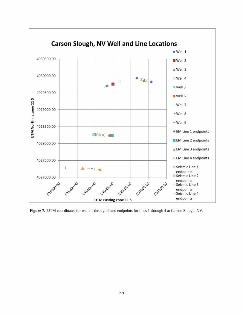
Locations of wells 1 through 9 and lines 1 through 4 can be found on Figure 7. Unified

soil classification system (USCS) symbols for various depths of Carson Slough wells 1 through 9

can be found on Table 2. It is clear from these classifications that the subsurface is fairly

heterogeneous (Figure 8), relative to the Palmyra site. Some layers are discontinuous,

segmented, and some are only present in a single well. Most of the wells contain swelling clays

toward the bottom. Some additional holes were augered and were rejected at hardened caliche

layers. The variation in water depths in the closely spaced wells was too great to be considered

as representing a simple unconfined system. Several additional investigative holes were augered

to determine if the system was confined and some areas had up to 4 ft (1.2 m) of pressure head

and some have none, showing that there are areas that are confined. These holes were not

augered during the time of geophysical data collection and water levels are transient in this area

so this pressure head could be different than pressure head at the time of geophysical data

acquisition. Table 3 shows the well data for depth to potentiometric surface and depth to

saturated layers where data are available.

Soil samples from wells 4 and 5 were used to make direct conductivity measurements

using a soil-water slurry. These measurements show that conductivity is higher in the lower

vadose zone than in the upper phreatic zone, and can be compared to EM modeled results

(Figure 9). Soil samples from well 4 were analyzed by XRD for quantification of minerals.

Major minerals include calcite, dolomite, illite, quartz, and anorthoclase feldspar.

14

EM Model Results

FEM results for Carson Slough were less consistent than those at Palmyra, as expected

due to the geological simplicity of the latter. Lines 1 and 2 are displayed (Figure 10 and 11) to

demonstrate conductivity profiles with shallow water at two different depths. There is a high

degree of variability in both magnitude and conductivity patterns over depth; however, they do

show that there is generally a conductivity high above the phreatic zone. The spacing between

the high and low conductivities is difficult to correlate to water surfaces because the depth to

water appears to be related to different parts of the conductivity trend depending on the location.

Modeled EM results for wells 4 and 5 are shown in Figure 11. Values from these models were

plotted next to measured values from soil samples for comparison on Figure 9. Additional EM

profiles for the other lines can be found in Appendix A-4. Modeled values for conductivity

range from 10-30 mS/m at the surface, to 250-500 mS/m in the mid-vadose zone, to 500-1000

mS/m at the peak above the vadose-phreatic boundary.

Seismic Results

Four seismic lines were included in this survey, but only profiles 1 and 2 are discussed as

mentioned above (Figures 12 and 13). The data ranges in quality from moderate to good, due

mainly to varying noise levels from wind, which usually increased throughout any day. Field

filters, stacking of multiple shot records, and data processing were used to help reduce the

influence of wind noise. Each of the four profiles shows shallow reflections in the depth range

expected for water levels observed in the wells.

Seismic reflections can usually be correlated with water level measurements from the

piezometers. However, these measurements may represent the pieziometric surface, and not the

15

actual depth to saturation, and thus the geophysical detection of groundwater (e.g., in a confined

aquifer) may indicate somewhat greater depths.

Profile 1, the northernmost of the four profiles (Figure 12), was surveyed over an active

drainage (but dry at the time of the survey) where water level depth in the well was minimal.

Shallow reflections with good continuity from the low-velocity field portion of the wave field

can be traced across the profile (Figure 12). The refraction model for this line (Figure 12-B)

appears to correlate reasonably well with a shallow reflection and measured water level in well 3.

Interpretations of depth to water surface from EM models are plotted on the seismic profile for

comparison (Figure 12-B). The EM interpretations show a higher degree of variably than the

seismic data with a discrepancy of up to 2 m.

Seismic Profile 2 is located just east of an intermittent stream (Figure 1-B) and traverses

an area where the water is considerably deeper than profile 1. The low-velocity field, above the

refraction model (Figure 13-B), produced poorly expressed reflectivity; however, the high-

velocity field, below the refraction model-based depth to a rigid surface (Figure 13) produced an

onset of stronger reflectivity arriving between 3 and 4 m below ground surface. Reflections for

profile 2 were less coherent and less continuous than those of profile 1. The pieziometric surface

at well 4 was at 2.8 m below ground and there appeared to be no pressure head. This depth

approximately matches the onset of reflectivity in the center of the profile. Depth to pieziometric

head at well 5, located on the west end of the profile, was 1.96 m and an additional investigative

hole was augered later and found that well 5 is in a confined system where depth to saturation is

2.26 m, shallower than the onset of reflectivity. The refraction model (Figure 13-B) shows that

the depth to the first rigid boundary changes from 4 m on the east end of the profile to < 1 m on

the west end. The upper layer on the east half of the profile could represent a fluvial channel,

16

which is consistent with its location in an ephemeral braided stream system. The dashed line

represents a possible second rigid layer at a depth of 3.8 m. Coherency of reflections above the

refraction model is lower than below it. EM interpretations to water surface are also plotted on

Figure 13-B and show more variability in depth than reflections, but less variability than the

refraction model; however, it corresponds fairly well with the second refraction boundary on the

west half of the profile.

DISCUSSION

The shallow water surfaces and elevated soil salinity create a challenging environment

for geophysical exploration of the groundwater system. Unconsolidated lacustrine and alluvial

sediments can result in rapid attenuation of acoustic energy and a well-developed capillary fringe

just above the phreatic zone can result in diminished velocity contrast by causing a gradational

change in velocity rather than a clear boundary. High soil salinity results in high conductivity,

which decreases the accuracy of EM measurements as depth increases (Callegary, et al., 2007).

Despite these problems the data show that EM and shallow seismic methods are promising in

measuring the configuration of the groundwater system when constrained by strategically

acquired ground truth.

The fact that the EM results varied considerably between the two sites in this

investigation suggests that the interpretation of EM data must be site specific. There is not a

universal conductivity that defines when a porous medium is saturated, nor is there a universal

trend of conductivity vs. depth. Local soil conditions must be taken into account to determine

depth to water when examining contrasts in conductivity vs. depth. If there is a significant

contrast in conductivity between the vadose and phreatic zones then these contrasts can be

17

interpreted to correlate to a water surface and their depth can be inferred from the Occam

inversion 1D profiles.

In arid areas with high concentrations of soluble salts in the soil, the conductivity of the

soil is dominated by salinity. Williams and Baker (1982) concluded that when measuring

apparent conductivity, salinity can account for 65-70% of the electromagnetic response.

Changes in subsurface conductivity are typically related to changes in the dominant factor (Cook

et al., 1992), which, in this case, is salinity. In both sites for this study there appeared to be a

conductivity high in the vadose zone and a drop in conductivity in the phreatic zone, although

the degree of change varies. At Carson Slough well 4 (Figure 9-A) the modeled change in

conductivity exceeds 800 mS/m and at Carson Slough well 5 (Figure 9-B) the modeled change in

conductivity is only 100 mS/m. This change in conductivity can be related to vertical changes in

salinity within the soil profile. Gilman and Bear (1994) confirmed that salinization of the vadose

zone is common in arid regions, particularly where water table is shallow, due to evaporation of

soil moisture. Dissolved salts present in small quantities in groundwater precipitate out into the

soil as the water is drawn up by capillary rise and evaporated (Forkutsa et al., 2009; Gilman and

Bear, 1994).

Salts were not concentrated enough in borehole samples to be measured with accuracy

using x-ray diffraction; however, quantification of salts, relative to other samples from the same

column, was achieved by a leaching experiment. The leachate from vadose zone samples show a

generalized increase in Na+ ion concentrations as depth increases and an abrupt drop in Na+ ion

concentration at the phreatic zone (Figure 4). This confirms the link between salinity in the soil

and conductivity measured either directly, or by electromagnetic response.

18

Small vertical fluctuations in Na+ ion concentration and fluctuations in directly measured

conductivity (Figures 3 and 9) were visible; however, the general trend for each set of

measurements is similar. The EM models do not show these small vertical fluctuations because

the nature of the soundings measures apparent conductivity over a given volume and the

Occam’s inversion produces a smooth model which cannot resolve minor fluctuations in a

general trend. Overall vertical trends can be picked up and modeled accurately in the case that

the subsurface is fairly horizontally homogeneous, such as at the Palmyra site.

At the Palmyra site, EM conductivity vs. depth profiles at each station were modeled and

analyzed. Each measurement in this line had a very similar electromagnetic response at its

respective depth. This is likely due to the laterally homogeneous soil profile and salinity

distribution. Because the aquifer is relatively homogeneous and unconfined, it is expected that

salinization due to capillary rise and evaporation would be consistent across the entire area

resulting in laterally comparable salinity concentrations. For this line the water table

corresponded to the point on the profile where conductivity drops from its peak. Using this

pattern, the depth to water was modeled across the line at a depth of 3 m, which is well within a

reasonable range of the piezometer water levels of 2.9 m at well 1 and 3.0 m at well 2.

EM interpretation at Carson Slough was more complex. Before EM models could be

understood, an interpretation of the subsurface needed to be made to know how conductivity

could vary over the profiles. Several factors contribute to the interpretation that the aquifer is not

a continuous system, but is made up of saturated channels flowing perpendicular to the profiles.

The variation in potentiometric surface over short lateral distances, in combination with the fact

that pressure head varies from 0 m to 1.2 m (Table 3) indicates that water systems are not

connected. Water temperature and conductivity are also inconsistent across single profiles

19

(Table 3). Water levels in several wells were measured 2 months after the collection of

geophysical data indicating that depth to water increased by varying amounts in wells 4 and 5,

but decreased by varying amounts in wells 1, 2, and 6 (Table 3). The current geologic setting of

the profiles is in an ephemeral river system that only flows at the surface after a storm (Tanko

and Glancy, 2001). It seems logical that the subsurface would contain buried channel systems at

various depths, some of which may or may not be confined by fine clays (Figure 14). A similar

arid environment with buried fluvial channels and fine clays can be found in the Okavango

Delta, Botswana (Milzo et al., 2009; Tooth and McCarthy, 2007)

Vertical salinity distribution in the Carson Slough area cannot be expected to be laterally

consistent where water surfaces, confining units, and soil types are not laterally consistent. For

this reason, conductivity distribution, although similar, is not consistent over the length of any of

the four EM profiles at Carson Slough (Figures 10 and 11). Although there is a conductivity

high above the saturated zone, in some cases the high is immediately above the water, as seen at

wells 1 and 2 at the Palmyra site (Figure 3), and in other cases it is 1-2 m above the water, as

seen at Carson Sough wells 4 and 5 (Figure 9). Because not enough piezometer control is

present to compare to each pattern of conductivity distribution, it is difficult to interpret an exact

depth to water with confidence. If depth to water is interpreted across an entire profile at the

point where conductivity drops, one can see that the depths are fairly inconsistent (Figure 15).

This is most likely influenced by the natural variations in depth to water across the profile, the

thickness of the saturated zones, and the seasonal fluctuations in depth to water. Seasonal

changes in water depths could result in perpetual vertical re-distribution of salinity. However,

since water levels measured at Carson Slough suggest that the amount of change, and even the

20

direction of change in water level varies across a short distance, the salinity re-distribution will

also vary laterally.

The complications of heterogeneity, segmented thin reservoirs, and seasonal water level

changes make FEM difficult to use for interpreting depth to water at Carson Slough unless

calibrating information such as occasional drill holes and /or seismic data are available. It

appears that using an interpretation that saturated depth corresponds with the depth where the

modeled conductivity drops from its peak is accurate to within approximately ± 2 m. This

uncertainly is difficult to gauge because it is directly proportional to water surface fluctuation

and heterogeneity in soil type and salinity concentration, which are poorly constrained in the

study area. However, because conductivity is linked to salinity, and soluble salts are more likely

to build up in areas where there is less direct communication with surface water, areas of higher

conductivity could be interpreted as areas with more confined systems, where areas with lower

conductivity could be interpreted as zones with greater surface water-ground water interaction.

The Palmyra site was essential in providing more of a “standard” site for exploring a

shallow water table in saline conditions, but with a more homogeneous geological setting. The

seismic profile at Palmyra was very successful in producing a simple reflection and head wave.

Despite the shallow nature of the target, and the possibility of the capillary fringe preventing

contrast in acoustic impedance at the water table, a strong reflection is apparent that corresponds

to the water depth as measured in the two piezometers (Figure 6-B). The resolution of the

seismic line is finer than that of the EM profiles, and because the CDP surface station spacing is

1 ft (~0.3 M) and EM stations were spaced at 10 m, the seismic line is far more complete for the

interval over which it was applied. As discussed above, the slight convex upward nature of the

reflection is a result of a slight concave nature of the ground surface over a constant water table.

21

This indicates that, relative to ground surface, depth to water is slightly less in the middle of the

line. This detail could not be resolved using the EM models, which were used to interpret a

depth of 3 m to water table across the entire line.

In the Carson Slough seismic profiles, shallow reflections, supported by velocity-depth

modeling of head waves and direct arrivals, indicate some correlation with depth to water in

piezometers on the lines (Figures 12 and 13). However, some piezometers have water levels that

do not correlate with any reflections. The profiles show that there is much more heterogeneity in

the Carson Slough area than in the Palmyra site. For example, shallow reflections produced

using the low-velocity field from Profile 1 show some undulation and curvature (Figure 12).

Reflections in profile 2 are discontinuous and truncated in places (Figure 13), which could be a

representation of buried stream channels flowing at a high angle to the profile. The seismic

method in Carson Slough is promising, although requires piezometer control and a priori

understanding of where confining units may be.

CONCLUSIONS

The testing of FEM and seismic methods to measure depth to groundwater in two

different areas allowed for comparison of the effectiveness of the methods in two arid to semi-

arid environments with elevated soil salinity that vary significantly in terms of subsurface

complexity. This allowed us to test the two end members of probable situations where these

methods could be useful while staying within the range of the project’s purpose to evaluate their

feasibility in arid saline conditions.

FEM soundings (Figures 5 and 11) were found to show similar patterns with

measurements taken from actual soil samples (Figures 3 and 9) at corresponding locations. The

magnitudes of conductivity from FEM models do not exactly match the conductivities measured

22

from soil samples. This is because measurements of conductivity in soil samples were made

using a slurry of equal mass of soil to water. Magnitude of the slurry conductivity is dependent

on the soil type, soluble salts, and dilution. The dilution prevents this method from measuring

the exact conductivity of the soil itself but, because the dilution was constant, it gives relative

magnitudes of the samples. This particular experiment was meant to show that the pattern of

conductivity over depth in EM models sufficiently matches direct measurements at various

depths, so relative magnitudes of conductivity were sufficient. The conductivity measurements

on soil samples indicate that there is an overall trend, but there are some minor fluctuations

within the overall conductivity trend (Figure 3), whereas FEM models show only the general

conductivity trend (Figure 5). Soil samples at the Carson Slough site were found to show less

similarity with their corresponding FEM profiles than those of the Palmyra site due to difficulty

in modeling the heterogeneous conditions at Carson Slough using FEM data.

FEM profiles show patterns of conductivity vs. depth that sufficiently correspond to

water table at the Palmyra site where the subsurface is fairly homogeneous. This homogeneity

allowed for accommodation of the entire horizontal range of the FEM sounding geometry to be

deployed without interference from zones of varying conductivity. The conductivity patterns

showed enough contrast between the phreatic and vadose zones to distinguish the boundary.

This contrast is due to salinization from capillary rise and evaporation: a process common to arid

areas with shallow water. At the Carson Slough site, EM profiles were more challenging to

interpret. The high degree of heterogeneity, both vertically, and horizontally, in combination

with the minimal piezometer control, large seasonal fluctuations in water depth, and segmented

thin reservoirs proved too complex to use FEM models to determine depth to water with the

same accuracy as at Palmyra.

23

Shallow high-resolution seismic methods (reflection and refraction) proved to be very

useful as a calibration and independent indicator of depth to saturation at both sites (especially

Palmyra, Figure 6). Seismic methods proved to have a higher resolution and showed a greater

degree of accuracy over the entire length of the profile than FEM results. The integration of the

two methods gives much more confidence in measurements of groundwater depth and

configuration when piezometer control is not present.

FEM soundings can be readily modeled to determine depth to shallow groundwater

where conditions are relatively horizontally homogeneous with sufficient salinization above the

saturated zone. This method would be very practical to use for a large-scale investigation. It has

the benefits of user-friendly instrumentation, rapid data collection, and is completely non-

invasive. However, because patterns in conductivity, not magnitude, are used to determine depth

to water it is necessary to have a calibration point where subsurface conditions change. This

could be either a piezometer with a well-documented log, or a shallow seismic profile with

sufficient resolution. The shallow high resolution profiles could also be used, but it is not

recommended for large areas due to the difficulty and time needed to acquire data of sufficient

resolution for shallow exploration.

24

REFERENCES

Al-Tarazi, E., Rajab, J.A., Al-Naqa, A., El-Waheidi, M., 2008, Detecting leachate plumes

and groundwater pollution at Ruseifa municipal landfill utilizing VLF-EM method: Journal of Applied Geophysics, v. 65, pp. 121-131.

Anderson, D.E., 2005, Holocene fluvial geomorphology of the Amargosa River through

Amargosa Canyon, California: Earth-Science Reviews, v. 73, pp. 291-307. Anderson, K.W., 2002, Contribution of local recharge to high flux springs in Death

Valley National Park, California-Nevada: Master’s thesis, Brigham Young University, 122 p.

Barnhurst, D.O., 2003, A chemical, stable, and radioisotopic investigation of an alluvial-fill groundwater system in a semi-arid environment, southern Utah Valley, Utah, Master’s thesis, Brigham Young University, 211 p.

Baker, G. S., Steeples, D. W., Schmeissner, C., and Spikes, K. T., 2000, Ultrashallow seismic

reflection monitoring of seasonal fluctuations in the water table: Environmental and Engineering Geoscience, vol. 6, pp. 271 - 277.

Bissell, H.J., 1963, Lake Bonneville: geology of southern Utah Valley, Utah: U.S. Geological

Survey Professional Paper 257-B, 35 p. Buselli, G., Davis, G.B., Barber, C., Heigt, M.I., and Howard, S.H.D., 1992, The application of

electromagnetic and electrical methods to groundwater problems in urban environments: Exploration Geophysics, v. 23, pp. 543-555.

Bushman, M., 2008, Contribution of recharge along regional flow paths to discharge at Ash

Meadows, Nevada, Master’s thesis, Brigham Young University, 119 p.

Callegary, J.B.; Ferre, T.P.A.; and Groom, R.W., 2007, Vertical spatial sensitivity and exploration depth of low-induction-number electromagnetic-induction instruments: Vadose Zone Journal, v. 6, pp. 158-167.

Clark, D.W., and Apple, C.L., 1985, Groundwater Resources of northern Utah Valley, Utah:

Utah Department of Natural Resources Technical Publication No. 80, 115 p. Classen, H.C., 1985, Sources and mechanisms of recharge for ground water in the west-central

Amargosa Desert, Nevada- a geochemical interpretation: U.S. Geological Survey Professional Paper 712-F.

Cockx, L. and De Vos, B., 2007, Using the EM38DD soil sensor to delineate clay lenses in a

sandy forest soil: Soil Science Society of America Journal, v. 71-4 pp. 1314-1321.

25

Constable, S.C., Parker, R.L., Constable, C.G., 1987, Occam’s inversion: a practical algorithm

for generating smooth models from electromagnetic sounding data: Geophysics, v. 52-3, p. 289-300.

Cook, P.G., Walker, G.R., Buselli, G., Potts, I., and Dodds, A.R., 1992, The application of

electromagnetic technique to groundwater recharge investigations: Journal of Hydrology, v. 107, pp. 251-265.

Doolittle, J.A., Sudduth, K.A., Kitchen, N.R., and Indorante, S.J., 1994, Estimating depths to

claypans using electromagnetic induction methods: Journal of Soil and Water Conservation, v. 49-6, pp. 572-575.

Eberl, D.D., 2003, User’s guide to RockJock – a program for determining quantitative

mineralogy from powder x-ray diffraction data: U.S. Geological Survey Open-File Report 03-78, 41 p.

Fitterman, D. V., Deszcz-Pan, M., Stoddard, C. E., 1999, Results of time-domain

electromagnetic soundings in Everglades National Park, Florida: U.S. Geological Survey, Open-File Report 99-426, pp. 155.

Fitterman, D. V., Stewart, M. T., 1986, Transient electromagnetic sounding for

groundwater: Geophysics, v. 51-4, pp. 995-1005. Forkutsa, I., Sommer, R., Shirokova, Y.I., Lamers, J.P.A., Kienzler, K., Tischbein, B., Martius,

C., and Vlek, P.L.G., 2009, Modeling irrigated cotton with shallow groundwater in the Aral Sea Basin of Uzbekistan: Irrigation Science, v. 27, pp. 319-330.

Grose, T., L., and Smith, G. I., 1989, Studies of geology and hydrology in the Basin and Range

Province, southwestern United States, for isolation of high-level radioactive waste— Characterization of the Death Valley Region, Nevada and California: U.S. Geological Survey Professional Paper 1370-F, pp. 5-19

Harrill, J.R., 1986, Ground-water storage depletion in Pahrump Valley, NevadaCalifornia,

1962-75: U.S. Geological Survey Water-Supply Paper 2279, 53 p. Hasselquist, N.J., and Allen, M.F., 2009, Increasing demands on limited water resources:

consequences for two endangered plants in Amargosa Valley, USA: American J. of Botany, v. 96-3, pp. 620-626.

Johnston, S.C. and T.A. Zink. 2003. Demographics and ecology of the Amargosa

niterwort (Nitrophila mohavensis) and Ash Meadows gumplant (Grindelia fraxino-pratensis) of the Carson Slough Area. Report to the Bureau of Land Management.

26

Kelly, W. E., and Mares, S. (Eds.) and Karous, M., Kelly, W. E., Landa, I., Mares, S., Mazac, O., Muller, K., Mullerova, J., 1993, Applied Geophysics in Hydrogeological and Engineering Practice: Elsevier, The Netherlands, 289 p.

Kilroy, K. C., 1991, Groundwater Conditions in Amargosa Desert, Nevada-California,

1952-1957: U.S. Geological Survey, (WRIR 89-4101). Laczniak and others, 1999, Estimates of Groundwater Discharge as Determined from

Measurements of Evapotranspiration , Ash Meadows Area, Nye County, Nevada: U.S. Geological Survey (WRIR 99-4079).

Louie, J., Shields, G., Ichinoise, G., Hasting, M., Plank, G., and Bowman, S., 1997, Shallow

geophysical constraints on displacement and segmentation of the Pahrump Valley Fault Zone, California-Nevada border: Submitted to Proceedings of the Basin and Range Province Seismic Hazards Summit for publication by the Utah Geological Survey, Cedar City, Utah. url: http://www.seismo.unr.edu/ftp/pub/louie/talks/lvsh/brshs-ed.pdf

Milzow, C., Kgotlhang, L., Kinzelbach, W., Meier, P., and Bauer-Gottwein, P., 2009, The role of

remote sensing in hydrological modeling of the Okavango Delta, Botswana: Journal of Environmental Management, v. 90, pp. 2252-2260.

Nabighian, M.N. and Corbett, J.D., (editors) 1991, Electromagnetic Methods in Applied

Geophysics: Society Of Exploration Geophysicists, Tulsa, Oklahoma, 992 p. Persson, M. and Haridy, S., 2003, Estimating water content from electrical conductivity

measurements with short time-domain reflectometry probes: Soil Science Society of America Journal, v. 67 pp. 478-482.

Potts, I. W., 1990, Use of the EM-34 instrument in groundwater exploration in the

Shepparton region: Australian Journal of Soil Research, v. 28, pp. 433-442. Reynolds, J.M., 1997, An Introduction to Applied and Environmental Geophysics: Wiley,

New York, 796 p. Rhoades, J.D., 1993, Electrical conductivity methods for measuring and mapping soil salinity:

Advances in Agronomy, v. 49, pp.201-251. Sada, D.W., 1990, Recovery plan for the endangered and threatened species of

Ash Meadows, Nevada: U. S. Fish and Wildlife Service, Portland. Sanderson, I.D. 2002, Ground-water sensitivity and vulnerability to pesticides, Utah and

Goshen Valleys, Utah County, Utah: Utah Geological Survey Miscellaneous Publication 02-10, 30 p.

27

Sengpiel, K., 1988, Results of airborne EM groundwater exploration in a desert area using the centroid depth algorithm for evaluation: Natuurwetenschappelijk Tijdschrift, v. 70, pp. 349-356.

Sheets, K.R., and Hendrickx, J.M.H., 1995, Noninvasive soil water content measurement

using electromagnetic induction: Water Resources Research, v. 31(10), pp. 2401-2409. Sparks, D.L., 2003, Environmental Soil Chemistry: Academic Press, San Diego, CA, 352 p. Stroh, J. C., Archer, S., Doolittle, J. A., and Wilding, L., 2001, Detection of edaphic

discontinuities with ground-penetrating radar and electromagnetic induction: Landscape Ecology, vol. 16, pp. 377-390.

Stonestrom, D.A., Prudic, D.E., Walvoord, M.A., Abraham, J.D., Stwart-Deaker, A.E., Glancy,

P.A., Constantz, J., Laczniak, R.J., and Andraski, B.J., 2007, Rocused ground-water recharge in the Amargosa Desert Basin: US Geological Survey Professional Paper 1703, p. 107-136

Sweetkind, D.S., Dikerson, R.P., Blakely, and R.J., Denning, P.D., 2001, Interpretive geologic

cross sections for the Death Valley regional flow system and surrounding areas, Nevada and California, US Geological Survey Miscellaneous Field Sudies Map MF-2370

Quittmeyer, R.C., 2000, Yucca Mountain site description: Prepared for U.S. Department of Energy, Prepared by TRW Environmental Safety Systems Inc., TDR-CRW-GS-000001 REV 01

Tan, K., Berens, V., Hatch, M., and Lawrie, K., 2007, Determining the suitability of in-stream

nanoTEM for delineating zones of salt accession to the River Murray: a review of survey results from Loxton, South Australia: Cooperative Research Centre for Landscape Environments and Mineral Exploration Open File Report, Report: 192, 24 p.

Tanko, D.J., and Glancy, P.A., 2001, Flooding in the Amargosa River drainage basin, February

23-24, 1998, southern Nevada and eastern California including the Nevada test site: US Geological Survey Fact Sheet 036-01.

Tooth, S., and McCarthy, T.S., 2007, Wetlands in drylands: geomorphological and

sedimentological characteristics, with emphasis on examples from southern Africa: Progress in Physical Geography, vol. 3, no. 1, pp. 3-41.

Urquhart, S., 2009, personal communication, Zonge Engineering, 3322 E Fort Lowell Rd

Tucson AZ, USA 85716 Utah Division of Water Resources, 1997, Utah state water plan, Utah Lake basin: Salt

Lake City, Utah Department of Natural Resources, 175 p.

28

Walker, G.E., and Eakin, T.E., 1963, Geology and Groundwater of the Amargosa Desert, Nevada-California: State of Nevada Department of Conservation and Natural Resources, Division of Water Resources, Water Resources Reconnaissance Series Report 14, 45 p.

Williams, B.G. and G.C. Baker. 1982, An electromagnetic induction technique for

reconnaissance surveys of soil salinity hazards: Australian Journal of Soil Research, v. 20, pp. 107-118.

Winograd, I. J., and Thordarson, W., 1975 Hydrogeologic and Hydrochemical

Framework, South-Central Great Basin, Nevada-California, with Special Reference to the Nevada Test Site: USGS Professional Paper 712-C.

Workman, J.B., Menges, C.M., Page, W.R., Taylor, E.M., Ekren, E.B., Rowley, P.D.,

Dixon, G.L., Thompson, R.A., and Write, L.A., 2001, Geologic map of the Death Valley ground-water model area, Nevada and California: U.S. Geological Survey Miscellaneous Field Studies map MF-2381-A, scale 1:250,000.

29

FIGURES

Figure 1. A) Location of EM and seismic reflection profiles for the line at the Palmyra, UT site. B) Location of EM and seismic reflection profiles for lines 1 through 4 at Carson Slough, Nevada site.

A

B

30

Figure 2. General soil profile for the Palmyra, UT site showing soil types and water table.

31

Figure 3. Conductivity measurements from augered holes at Palmyra, UT site. A) Conductivity vs. depth for well 1 where measured depth to water is 9.5 ft. (2.9 m). Blue curve is measured from soil samples in laboratory. Red curve is taken from modeled EM profiles. Red line indicates depth to water table. B) Conductivity vs depth for well 2 where measured depth to water is 9.8 ft. (3.0 m). Blue curve is measured from soil samples in laboratory. Red curve is taken from modeled EM profiles. All conductivity measurements were made with a YSI conductivity meter from a slurry of 30g of sample with 30 mL of de-ionized water.

0

1

2

3

4

5

6

10 510 1010 1510 2010

Dep

th m

Conductivity mS/m

Palmyra Well 1 Conductivity vs Depth

Direct

Modeled

0

0.5

1

1.5

2

2.5

3

3.5

4

4.5

5

10 510 1010 1510

Dep

th m

Conductivity mS/m

Palmyra Well 2 Conductivity vs Depth

Direct

Modeled

32

Figure 4. AA analysis of Na+ concentrations from leachate experiment with soil samples from Palmyra well 1. Red line indicates depth to water table. Dashed line indicates smoothed conductivity trend.

00.5

11.5

22.5

33.5

4

0 500 1000 1500 2000 2500

Dep

th m

Na+ ion concentration mg/L

Palmyra Well 1 Na+ ion concentration vs depth

33

Figure 5. A) EM conductivity vs. depth model for Palmyra well 1 located at station 2 on the profile in Figure 5C. Red line indicates water table. B) EM conductivity vs. depth model for Palmyra well 2 located at station 8 on Figure 5C. Red line indicates water table. C) Profile of EM conductivity data for the entire line with stations 1-10 from left to right. The upper portion indicates conductivity magnitude and distribution of the 12 measurements per station. The lower portion shows the conductivity trend over depth.

C

B A

34

Figure 6. A) Processed seismic line for Palmyra site with fold of cover indicated at the top. Source and receiver spacing is 1 ft (0.3047 m) and CDP spacing is 0.5 ft (0.1524 m). B) Seismic profile for Palmyra site with location of two wells with their corresponding measured depth to water marked by green line with triangle. EM interpretation of depth to water is marked by the light-blue line. Dashed black line represents depth to first rigid layer determined by refraction models from the shot records.

A

B

35

Figure 7. UTM coordinates for wells 1 through 9 and endpoints for lines 1 through 4 at Carson Slough, NV.

4027000.00

4027500.00

4028000.00

4028500.00

4029000.00

4029500.00

4030000.00

4030500.00

UTM

Nor

thin

g zo

ne 1

1 S

UTM Easting zone 11 S

Carson Slough, NV Well and Line LocationsWell 1

Well 2

Well 3

Well 4

well 5

well 6

Well 7

Well 8

Well 9

EM Line 1 endpoints

EM Line 2 endpoints

EM Line 3 endpoints

EM Line 4 endpoints

Seismic Line 1 endpointsSeismic Line 2 endpointsSeismic Line 3 endpointsSeismic Line 4 endpoints

36

Figure 8. Generalized soil profile for Line 2 at Carson Slough, NV site. Soil column is complex and heterogeneous. Water table is inconsistent

37

Figure 9. Conductivity measurements from augered adjacent to wells 4 and 5 at Carson Slough, NV. A) Conductivity vs. depth for well 2 where measured depth to pieziometric surface and saturation are both 9.2 ft. (2.8 m) represented by the red line. Blue curve is measured from soil samples in laboratory. Red curve is taken from modeled EM profiles. B) Conductivity vs. depth for well 5 where measured depth to pieziometric surface is 6.4 ft. (2.0 m) and saturation is at 2.25 m represented by the upper and lower red lines respectively. Blue curve is measured from soil samples in laboratory. Red curve is taken from modeled EM profiles. All conductivity measurements were made with a YSI conductivity meter from a slurry of 30g of sample with 30 mL of de-ionized water.

0

0.5

1

1.5

2

2.5

3

3.5

4

4.5

10 210 410 610 810 1010 1210

Dep

th m

Conductivity mS/m

Carson Slough Well 4 Conductivity vs Depth

Direct

Modeled

0

0.5

1

1.5

2

2.5

3

3.5

4

10 110 210 310 410 510 610

Dep

th m

Conductivity mS/m

Carson Slough Well 5 Conductivity vs Depth

Direct

Modeled

A

B

38

Figure 10. EM conductivity profile for line 1 with stations 1 thorugh 20 from left to right. Station 1 is in the northwest end of the line and station 20 is on the southeast end of the line. The upper portion indicates conductivity magnitude and distribution of the 12 measurements per station. The lower portion shows the conductivity trend over depth.

39

Figure 11. A) EM conductivity vs. depth model for Carson Slough well 4 located at station 3 on Line 2. The red line indicates saturation at 2.9 m. B) EM conductivity vs. depth model for Carson Slough well 5 located at station 11 on Line 2. The upper and lower red lines indicate the potentiometric surface and saturated depth at 2.0 and 2.3 m, respectively.

B A

40

Figure 12. A) Seismic profile 1 at Carson Slough site. Source and receiver spacing is 1 ft (0.3047 m) and CDP spacing is 0.5 ft (0.1524 m). B) Seismic profile for Carson Slough profile 1 with location of wells 4 and its corresponding measured depth to water marked by green line with triangle. EM interpretation is of depth to water are marked by the light blue line with satation 13 on the left to station 9 on the right. Yellow line represents depth to first rigid layer determined by refraction models from the shot records.

A

B

41

Figure 13. A) Stacked section for Carson Slough profile 2. Source and receiver spacing is 1 ft (0.3047 m) and CDP spacing is 0.5 ft (0.1524 m). B) Seismic profile for Carson Slough profile 2 with location of wells 4 and its corresponding measured depth to water marked by green line with triangle. EM interpretation is of depth to water are marked by the light blue line with satation 1 on the left to station 7 on the right. Yellow line represents depth to first rigid layer determined by refraction models from the shot records. Dashed yellow line represents a possible second rigid layer.

B

A

42

Figure 14. Interpretation of Carson Slough subsurface composed of fine grained channels surrounded by a matrix of clays and other fine grain sediments and sands, with a topographic map from Figure 1-B of the Carson Slough area on top.

Figure 15. Depth to water using an interpretation where depth to water is at the point immediately below the conductivity peak for Line 2 at Carson Slough. Interpreted using individually modeled station (as opposed to modeling as a profile). Each station is 10 m apart

0.00

1.00

2.00

3.00

4.00

0 1 2 3 4 5 6 7 8 9 10 11 12 13 14 15 16 17 18 19 20 21 22 23

Dep

th to

wat

er (m

)

station

Interpreted Depth to water from EM models-Carson Slough Line 2

43

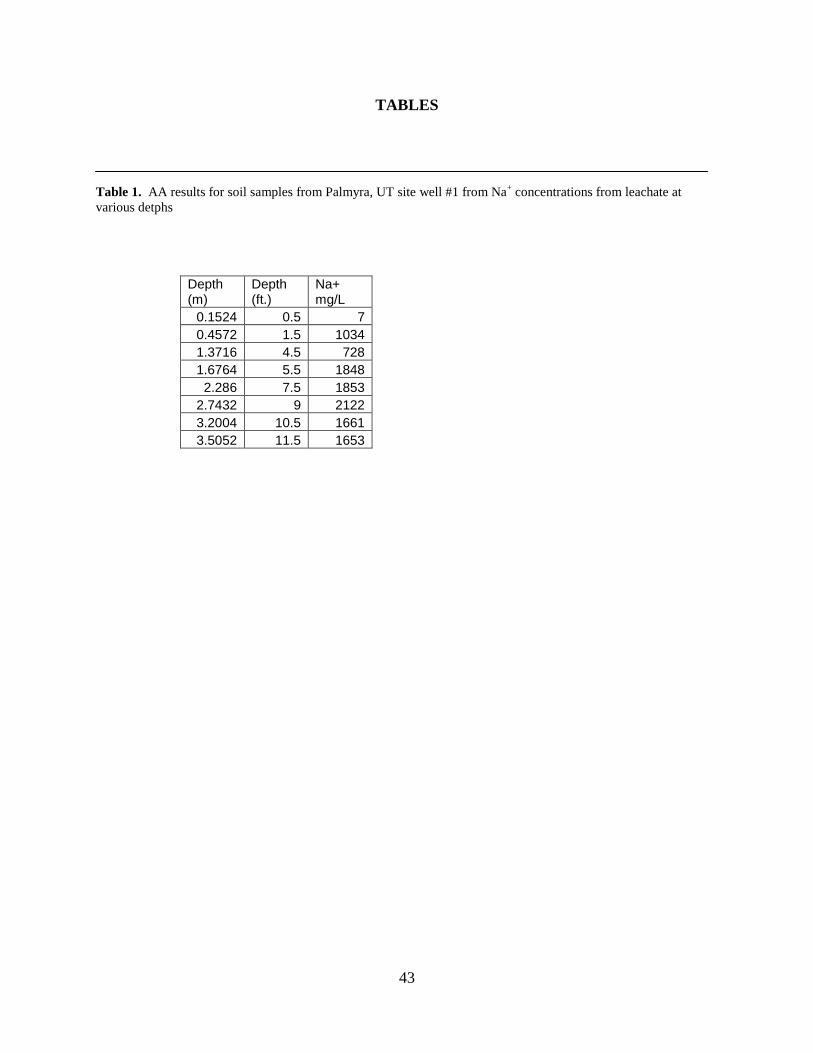
TABLES

Table 1. AA results for soil samples from Palmyra, UT site well #1 from Na+ concentrations from leachate at various detphs

Depth (m)

Depth (ft.)

Na+ mg/L

0.1524 0.5 7 0.4572 1.5 1034 1.3716 4.5 728 1.6764 5.5 1848 2.286 7.5 1853

2.7432 9 2122 3.2004 10.5 1661 3.5052 11.5 1653

44

Table 2. Data from augered holes at both the Palmyra, UT and Carson Slough, NV sites. Depth to water for the Palmyra site is to water table. Depth to water for Carson Slough wells is to potentiometric surface. Soil classification abbreviations are listed at the end.

Palmyra well 1 USCS classification symbol

Palmyra well 2 USCS classification symbol

Carson Slough well 1 USCS classification symbol

Carson Slough well 2 USCS classification symbol

Ground elevation (ft.) 2135.4 2130.9 Depth to water 9.5 9.8 10.1 4.6 Line line 4 line 4 Depth interval

0.0 to 1 ML ML SP-SM SP-SM 1.0 to 1.5 ML ML SP-SM SP-SM 1.5 to 2 ML ML SP-SM SP-SM 2.0 to 2.5 ML ML SP-SM SC 2.5 to 3 ML ML SP-SM SC 3.0 to 3.5 ML ML SP-SM SC 3.5 to 4 ML ML SP-SM SC 4.0 to 4.5 ML ML SC SC 4.5 to 5 ML ML SC SC 5.0 to 5.5 ML ML SC CL 5.5 to 6 ML ML SC CL 6.0 to 6.5 ML ML SC CL 6.5 to 7 ML ML SC CL 7.0 to 7.5 SM SM SC CL 7.5 to 8 SM SM SC CL 8.0 to 8.5 ML ML SC CL 8.5 to 9 ML ML SC CL 9.0 to 9.5 ML ML CL 9.5 to 10 ML ML CL

10.0 to 10.5 ML ML CL 10.5 to 11 ML ML CL 11.0 to 11.5 ML ML CL 11.5 to 12 ML ML CL 12.0 to 12.5 CL 12.5 to 13 CL

45

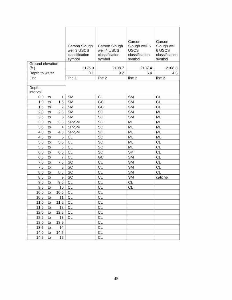
Carson Slough well 3 USCS classification symbol

Carson Slough well 4 USCS classification symbol

Carson Slough well 5 USCS classification symbol

Carson Slough well 6 USCS classification symbol

Ground elevation (ft.) 2126.0 2108.7 2107.4 2108.3 Depth to water 3.1 9.2 6.4 4.5 Line line 1 line 2 line 2 line 2 Depth interval

0.0 to 1 SM CL SM CL 1.0 to 1.5 SM GC SM CL 1.5 to 2 SM GC SM CL 2.0 to 2.5 SM SC SM ML 2.5 to 3 SM SC SM ML 3.0 to 3.5 SP-SM SC ML ML 3.5 to 4 SP-SM SC ML ML 4.0 to 4.5 SP-SM SC ML ML 4.5 to 5 CL SC ML ML 5.0 to 5.5 CL SC ML CL 5.5 to 6 CL SC ML CL 6.0 to 6.5 CL SC SP CL 6.5 to 7 CL GC SM CL 7.0 to 7.5 SC CL SM CL 7.5 to 8 SC CL SM CL 8.0 to 8.5 SC CL SM CL 8.5 to 9 SC CL SM caliche 9.0 to 9.5 CL CL CL 9.5 to 10 CL CL CL

10.0 to 10.5 CL CL 10.5 to 11 CL CL 11.0 to 11.5 CL CL 11.5 to 12 CL CL 12.0 to 12.5 CL CL 12.5 to 13 CL CL 13.0 to 13.5 CL 13.5 to 14 CL 14.0 to 14.5 CL 14.5 to 15 CL

46

Carson Slough well 7 USCS classification symbol

Carson Slough well 8 USCS classification symbol

Carson Slough well 9 USCS classification symbol

Ground elevation (ft.) 2096.0 2096.8 2095.8 Depth to water 15.4 7.8 5.7 Line not on a line line 3 line 3 Depth interval

0.0 to 1 SW-SC SC SW-SC 1.0 to 1.5 SW-SC SC SW-SC 1.5 to 2 SW-SC SC SW-SC 2.0 to 2.5 SW-SC SC CL 2.5 to 3 SW-SC SC CL 3.0 to 3.5 SW-SC SC CL 3.5 to 4 SW-SC SC CL 4.0 to 4.5 SW-SC CL SW-SC 4.5 to 5 SW-SC CL SW-SC 5.0 to 5.5 SW-SM CL SC 5.5 to 6 SW-SM CL SC 6.0 to 6.5 SW-SM CL SC 6.5 to 7 SW-SM CL SC 7.0 to 7.5 CL CL SW 7.5 to 8 CL CL SW 8.0 to 8.5 CL CL 8.5 to 9 CL CL 9.0 to 9.5 CL CL 9.5 to 10 CL CL

10.0 to 10.5 CL CL 10.5 to 11 CL CL 11.0 to 11.5 CL CL 11.5 to 12 CL CL 12.0 to 12.5 CL CL 12.5 to 13 CL CL 13.0 to 13.5 CL 13.5 to 14 CL 14.0 to 14.5 CL 14.5 to 15 CL 15.0 to 15.5 CL 15.5 to 16 CL

CL= Clay; GC= Clayey Gravel; ML= Silt; SC= Clayey Sand; SM= Silty Sand; SP= Poorly Graded Sand; SW= Well Graded Sand

47

Table 3. Data for wells 1-9 in the Carson Slough, Nevada area (CS) plus an additional borehole (BH) and wells 1-2 at Palmyra, Utah (P). All data is from August 31, 2007 except for the last two rows which are from Sept. 25, 2007 and and the two columns for Palmyra, UT wells which are from October, 2008.

ID CS well 1 CS well 2 CS well 3 CS well 4 CS well 5 CS well 6 Aug. 31, 2007 UTM easting 556534.80 556599.00 556947.94 556410.33 556489.25 556563.32 UTM northing 4029705.66 4029758.00 4029877.22 4028259.80 4028250.98 4028236.22 Well Depth (ft.) 13.5 9.74 13.21 18.80 11.14 9.90 Temperature C 23.8 25.2 25.8 21.6 26.4 no data pH 7.83 7.82 8.04 7.86 7.63 no data Conductivity mS/m 84.8 234 396 619 627 no data Water Elevation (ft) 2125.27 2126.32 2122.85 2099.48 2100.95 2103.73 Depth to Water (ft.) 10.1 4.6 3.1 9.2 6.4 4.5 Depth to Water (m) 3.08 1.41 0.96 2.82 1.96 1.38 Pressure Head no data 1.50 no data 0.00 1.00 0.00 Sept. 25, 2007 Water depth (ft.) 10.6 5.05 no data 8.14 5.97 7.22 Change in Water elevation (ft.) -0.49 -0.44 no data 1.10 0.45 -2.68

ID CS well 7 CS well 8 CS well 9 CS BH-1 P well 1 P well 2 Aug. 31, 2007

UTM easting 556068.97 556357.50 556446.49 556422.54 UTM northing 4027279.39 4027252.50 4027232.76 4028346.90 Well Depth (ft.) 16.50 12.01 9.10 14.30 Temperature C no data 24.8 30.1 21.8 pH no data 8.45 7.95 8.11 Conductivity uS/m no data 1330 1640 381 5310 Water Elevation (ft) 2080.62 2088.98 2090.13 2100.16 Depth to Water (ft.) 15.4 7.8 5.7 7.6 9.4 9.7 Depth to Water (m) 4.69 2.39 1.74 2.32 2.9 3.0 Pressure Head no data no data no data 4.00 0.0 0.0 Sept. 25, 2007

Water depth (ft.) no data no data no data no data

Change in Water Level (ft.) no data no data no data no data

48

APPENDIX A

49

Appendix A-1. XRD RockJock analyses showing approximate mineralogy for samples from the Palmyra, UT site well #1.

Sample name: P1 1.5 P1 4.5 P1 5.5 P1 7.5 P1 9.0 P1 10.5 P1 11.5

Full pattern degree of fit: 0.185 0.172 0.175 0.227 0.158 0.161 0.211

Mineral Weight % Weight % Weight % Weight % Weight % Weight % Weight % NON-CLAYS

Quartz 42.2 44.8 35.2 45.3 23.9 43.2 58 Anorthoclase feldspar 8.4 8.1 11.9 17.7 7.3 10.7 13.1

Calcite 39.9 14.3 24.9 13.8 29.5 21.6 14.5 Dolomite 9.5 3.8 6.6 4.2 5.2 6 3.6 Mordenite 0 14.6 2.4 12.5 10 1.8 6.4

Total non-clays 100 85.6 81 93.6 76 83.2 95.6

CLAYS

Na-Smectite (Wyo) 0 14.4 19 6.4 24 16.8 4.4

Total clays 0 14.4 19 6.4 24 16.8 4.4

TOTAL 100 100 100 100 100 100 100

Appendix A-2. XRD RockJock analyses showing approximate mineralogy for samples from the Carson Slough site well #4.

Sample name: CS4 1.6

CS4 3.3

CS4 4.5

CS4 5.8

CS4 6.8

CS4 7.8

CS4 9.0

CS4 9.8

CS4 10.7

CS4 12.1

Full pattern degree of fit: 0.159 0.139 0.14 0.168 0.163 0.139 0.156 0.143 0.143 0.164

Mineral Weight

% Weight

% Weight

% Weight

% Weight

% Weight

% Weight

% Weight

% Weight

% Weight

% NON-CLAYS

Quartz 14.6 1.8 6.9 16.7 20.7 6.2 1.7 0.9 2.2 16.9 Sanidine feldspar 10.9 16.6 8.3 16.2 18.3 14.2 12.8 18.3 18.9 13.8

Anorthoclase feldspar 38 13.7 28.7 51.5 42.5 22.7 19.9 17 19.7 44.1 Calcite 28.9 15.5 53.9 9.5 0.7 3 1.4 2 3.8 20.7

Dolomite 1.7 24.4 1.6 0.2 0.5 36.8 44.2 39.4 27.8 1.4

Total non-clays 94.1 72 99.4 94 82.7 82.9 80 77.6 72.4 96.8

CLAYS Illite 5.9 28 0.6 6 17.3 17.1 20 22.4 27.6 3.2

Total clays 5.9 28 0.6 6 17.3 17.1 20 22.4 27.6 3.2

TOTAL 100 100 100 100 100 100 100 100 100 100

50

Appendix A-3. Raw EM conductivity data for line at Palmyra, UT and the 4 lines at Carson Slough

Instrument --> EM-38 EM-38 EM-38 EM-38 EM-31-SH EM-31-SH EM-31-SH EM-31-SH EM-34 EM-34 EM-34 EM-34

Frequency --> 14600 Hz 14600 Hz 14600 Hz 14600 Hz 9800 Hz 9800 Hz 9800 Hz 9800 Hz 6400 Hz 6400 Hz 1600 Hz 1600 Hz

coil separation --> 1m 1m 1m 1m 2m 2m 2m 2m 10m 10m 20m 20m

Dipole oridentation --> veritcal horizontal veritcal horizontal veritcal horizontal veritcal horizontal veritcal horizontal veritcal horizontal

height above ground -> 1.0 m 1.0 m 0 0 0.95 0.95 0 0 0 0 0 0

UTM easting Zone 11S

UTM northing zone 11S

elevation (feet)

elevation (meters) mS/m mS/m mS/m mS/m mS/m mS/m mS/m mS/m mS/m mS/m mS/m mS/m

Palmyra, UT Station #

1 95 48 246 174 249 141 422 294 44 238 32 224

(well 1) 2 88 43 221 132 247 135 407 261 38 238 45 241

3 92 45 235 135 248 129 431 260 41 240 34 238

4 93 45 232 142 248 135 427 270 45 233 26 226

5 90 43 221 134 246 130 412 260 49 219 36 226

6 87 42 213 126 229 123 391 242 50 224 45 221

7 89 43 225 131 235 127 406 258 59 220 40 219

(well2) 8 93 46 222 139 237 138 389 257 65 220 36 219

9 97 47 237 142 254 138 438 278 37 236 25 221

10 114 57 300 213 291 162 480 351 35 240 13 233

Carson Slough Station #

Line 1 1 556866.8 4029935.08 2130.16 649.2741 58 28 190 129 127 71 205 176 48 134 63 146

Line 1 2 556874.83 4029929.34 2129.3 649.0119 53 27 163 121 125 71 203 169 71 133 64 144

Line 1 3 556883.01 4029923.59 2129.97 649.2162 55 28 182 123 126 77 226 184 34 135 64 135

Line 1 4 556891.09 4029917.73 2129.28 649.0058 33 15 82 54 91 47 143 90 82 116 66 135

Line 1 5 556899.15 4029911.9 2129.55 649.0881 46 23 147 118 103 65 147 153 57 120 93 128

Line 1 6 556907.32 4029906.18 2129.41 649.0455 51 26 161 134 118 67 167 160 65 120 72 136

Line 1 7 556915.41 4029900.39 2129.27 649.0028 58 29 189 161 132 79 200 192 49 123 55 137

Line 1 8 556923.56 4029894.57 2128.79 648.8565 57 30 174 159 134 79 187 206 70 119 80 141

Line 1 9 556931.79 4029888.82 2128.46 648.7559 67 34 232 199 142 91 194 227 52 124 71 139

Line 1 10 556939.9 4029883.17 2127.55 648.4785 62 31 194 156 143 83 223 205 51 135 62 142

Line 1 (Well 3)

11 556947.94 4029877.22 2125.99 648.0031 59 31 135 175 135 84 160 198 76 137 84 148

Line 1 12 556956.05 4029871.44 2125.93 647.9848 68 36 200 223 144 92 146 243 92 139 88 157

Line 1 13 556964.22 4029865.61 2127 648.3109 72 37 213 182 168 97 261 233 54 156 50 164

Line 1 14 556972.36 4029859.84 2127.66 648.5121 88 46 296 221 206 119 313 292 48 182 30 177

Line 1 15 556980.5 4029854.08 2128.47 648.759 84 44 270 217 206 127 335 316 35 199 38 188

Line 1 16 556988.61 4029848.17 2127.76 648.5426 99 51 331 264 234 137 357 354 59 190 52 190

Line 1 17 556996.75 4029842.47 2128.83 648.8687 75 38 206 137 193 109 326 242 48 190 48 198

Line 1 18 557004.87 4029836.66 2128.61 648.8016 89 45 276 173 240 133 422 291 37 216 14 216

51

Line 1 19 557013.1 4029830.86 2127.6 648.4938 134 67 408 301 327 181 532 455 5 245 5 232

Line 1 20 557021.18 4029825.08 2127.28 648.3962 141 74 487 387 332 200 520 522 13 250 17 244

Line 1 21 557029.34 4029819.39 2127.1 648.3414 167 87 592 507 374 230 589 634 0 252 50 244

Line 2 1 556390.51 4028262.15 2108.47 642.6629 85 43 279 192 218 129 361 307 33 206 49 203

Line 2 2 556400.39 4028260.92 2108.56 642.6904 83 39 275 141 220 119 440 267 57 202 26 182

Line 2 (well 4) 3 556410.33 4028259.8 2108.72 642.7391 63 31 186 129 164 99 274 229 81 172 83 162

Line 2 4 556420.23 4028258.58 2108.68 642.727 51 23 135 78 142 75 238 148 129 127 72 151

Line 2 5 556430.15 4028257.46 2108.56 642.6904 52 23 138 80 141 77 237 158 117 137 105 151

Line 2 6 556440.1 4028256.5 2108.01 642.5227 75 38 249 158 185 109 329 252 64 173 66 160

Line 2 7 556450.01 4028255.52 2107.9 642.4892 111 59 410 363 249 153 351 415 33 184 52 164

Line 2 8 556459.93 4028254.45 2108.2 642.5807 89 44 298 205 215 122 358 290 72 183 48 166

Line 2 9 556469.8 4028253.09 2108.4 642.6416 71 36 222 177 170 104 264 243 85 163 64 157

Line 2 10 556479.78 4028252 2108.07 642.541 55 27 169 112 141 82 234 176 70 148 73 154

Line 2 (well 5) 11 556489.25 4028250.98 2107.37 642.3277 48 22 136 80 126 68 221 149 78 135 79 152

Line 2 12 556499.56 4028249.85 2107.87 642.4801 37 17 100 56 108 58 185 114 82 132 76 150

Line 2 13 556509.47 4028248.82 2108.38 642.6355 34 17 88 58 96 55 152 108 122 127 103 150

Line 2 14 556519.45 4028247.81 2110.17 643.1811 43 21 99 59 111 61 175 117 67 130 110 149

Line 2 15 556529.34 4028246.54 2109.68 643.0318 73 36 226 156 175 100 300 242 38 160 46 152

Line 2 16 556539.26 4028245.41 2108.26 642.5989 93 50 264 281 218 130 295 316 68 198 50 159

Line 2 17 556549.09 4028244.33 2108.75 642.7483 68 34 208 150 162 92 255 203 108 161 88 165

Line 2 18 556559.05 4028243.31 2108.28 642.605 68 34 208 150 162 92 255 203 108 161 88 165

Line 2 19 556568.98 4028242.13 2108.33 642.6203 74 38 223 154 187 102 321 233 61 176 76 159

Line 2 20 556578.81 4028241.02 2109.34 642.9281 64 33 197 132 162 95 272 210 49 177 75 157

Line 2 21 556588.74 4028239.72 2110.06 643.1476 51 25 143 92 131 75 224 164 65 159 69 151

Line 3 1 556259.98 4027274.43 2098.33 639.5723 78 40 249 143 214 115 385 250 56 203 46 202

Line 3 2 556269.73 4027272.19 2098.27 639.554 80 38 224 138 213 112 373 239 38 199 58 203

Line 3 3 556279.48 4027269.99 2098.66 639.6729 72 38 205 126 193 111 340 242 69 209 41 197

Line 3 4 556289.26 4027267.81 2098.43 639.6027 70 33 167 103 190 101 333 196 59 180 40 191

Line 3 5 556299 4027265.67 2097.98 639.4656 62 31 159 94 169 90 285 184 73 177 54 181

Line 3 6 556308.77 4027263.5 2097.13 639.2065 46 23 108 64 128 72 213 133 76 165 81 179

Line 3 7 556318.57 4027261.24 2097.02 639.173 44 21 105 62 127 67 205 123 76 155 86 176

Line 3 8 556328.34 4027259.18 2097.45 639.304 46 22 115 67 129 70 214 130 67 158 65 182

Line 3 9 556337.94 4027256.87 2097.07 639.1882 53 26 133 80 145 82 244 154 88 176 88 185

Line 3 10 556347.71 4027254.73 2097.37 639.2797 54 26 119 72 149 83 235 148 57 184 70 192

Line 3 (well 8) 11 556357.5 4027252.5 2096.83 639.1151 78 39 229 145 204 112 324 247 79 189 76 195

Line 3 12 556367.29 4027250.26 2097.36 639.2766 89 45 269 174 230 128 393 288 43 197 29 199

Line 3 13 556376.99 4027247.97 2097.76 639.3985 71 36 208 132 187 102 317 220 68 196 49 203

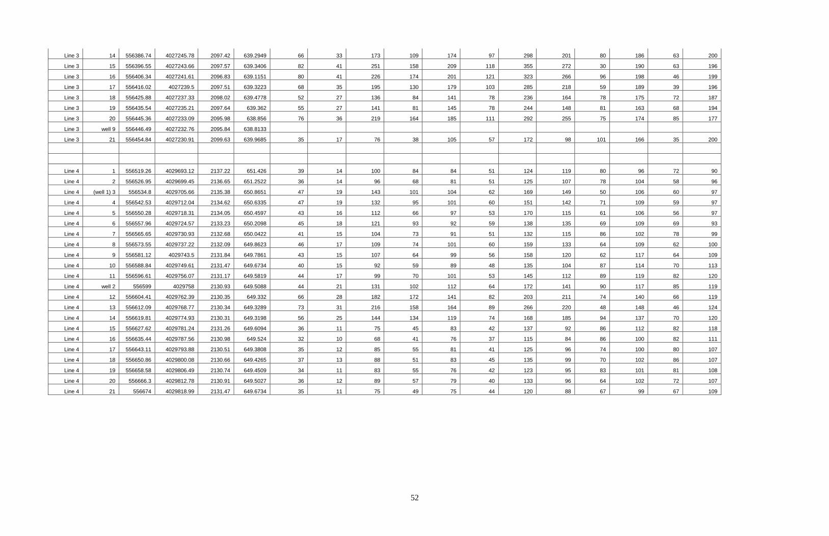
52

Line 3 14 556386.74 4027245.78 2097.42 639.2949 66 33 173 109 174 97 298 201 80 186 63 200

Line 3 15 556396.55 4027243.66 2097.57 639.3406 82 41 251 158 209 118 355 272 30 190 63 196

Line 3 16 556406.34 4027241.61 2096.83 639.1151 80 41 226 174 201 121 323 266 96 198 46 199

Line 3 17 556416.02 4027239.5 2097.51 639.3223 68 35 195 130 179 103 285 218 59 189 39 196

Line 3 18 556425.88 4027237.33 2098.02 639.4778 52 27 136 84 141 78 236 164 78 175 72 187

Line 3 19 556435.54 4027235.21 2097.64 639.362 55 27 141 81 145 78 244 148 81 163 68 194

Line 3 20 556445.36 4027233.09 2095.98 638.856 76 36 219 164 185 111 292 255 75 174 85 177

Line 3 well 9 556446.49 4027232.76 2095.84 638.8133

Line 3 21 556454.84 4027230.91 2099.63 639.9685 35 17 76 38 105 57 172 98 101 166 35 200

Line 4 1 556519.26 4029693.12 2137.22 651.426 39 14 100 84 84 51 124 119 80 96 72 90

Line 4 2 556526.95 4029699.45 2136.65 651.2522 36 14 96 68 81 51 125 107 78 104 58 96

Line 4 (well 1) 3 556534.8 4029705.66 2135.38 650.8651 47 19 143 101 104 62 169 149 50 106 60 97

Line 4 4 556542.53 4029712.04 2134.62 650.6335 47 19 132 95 101 60 151 142 71 109 59 97

Line 4 5 556550.28 4029718.31 2134.05 650.4597 43 16 112 66 97 53 170 115 61 106 56 97

Line 4 6 556557.96 4029724.57 2133.23 650.2098 45 18 121 93 92 59 138 135 69 109 69 93

Line 4 7 556565.65 4029730.93 2132.68 650.0422 41 15 104 73 91 51 132 115 86 102 78 99

Line 4 8 556573.55 4029737.22 2132.09 649.8623 46 17 109 74 101 60 159 133 64 109 62 100

Line 4 9 556581.12 4029743.5 2131.84 649.7861 43 15 107 64 99 56 158 120 62 117 64 109

Line 4 10 556588.84 4029749.61 2131.47 649.6734 40 15 92 59 89 48 135 104 87 114 70 113

Line 4 11 556596.61 4029756.07 2131.17 649.5819 44 17 99 70 101 53 145 112 89 119 82 120

Line 4 well 2 556599 4029758 2130.93 649.5088 44 21 131 102 112 64 172 141 90 117 85 119

Line 4 12 556604.41 4029762.39 2130.35 649.332 66 28 182 172 141 82 203 211 74 140 66 119

Line 4 13 556612.09 4029768.77 2130.34 649.3289 73 31 216 158 164 89 266 220 48 148 46 124

Line 4 14 556619.81 4029774.93 2130.31 649.3198 56 25 144 134 119 74 168 185 94 137 70 120

Line 4 15 556627.62 4029781.24 2131.26 649.6094 36 11 75 45 83 42 137 92 86 112 82 118

Line 4 16 556635.44 4029787.56 2130.98 649.524 32 10 68 41 76 37 115 84 86 100 82 111

Line 4 17 556643.11 4029793.88 2130.51 649.3808 35 12 85 55 81 41 125 96 74 100 80 107

Line 4 18 556650.86 4029800.08 2130.66 649.4265 37 13 88 51 83 45 135 99 70 102 86 107

Line 4 19 556658.58 4029806.49 2130.74 649.4509 34 11 83 55 76 42 123 95 83 101 81 108

Line 4 20 556666.3 4029812.78 2130.91 649.5027 36 12 89 57 79 40 133 96 64 102 72 107

Line 4 21 556674 4029818.99 2131.47 649.6734 35 11 75 49 75 44 120 88 67 99 67 109

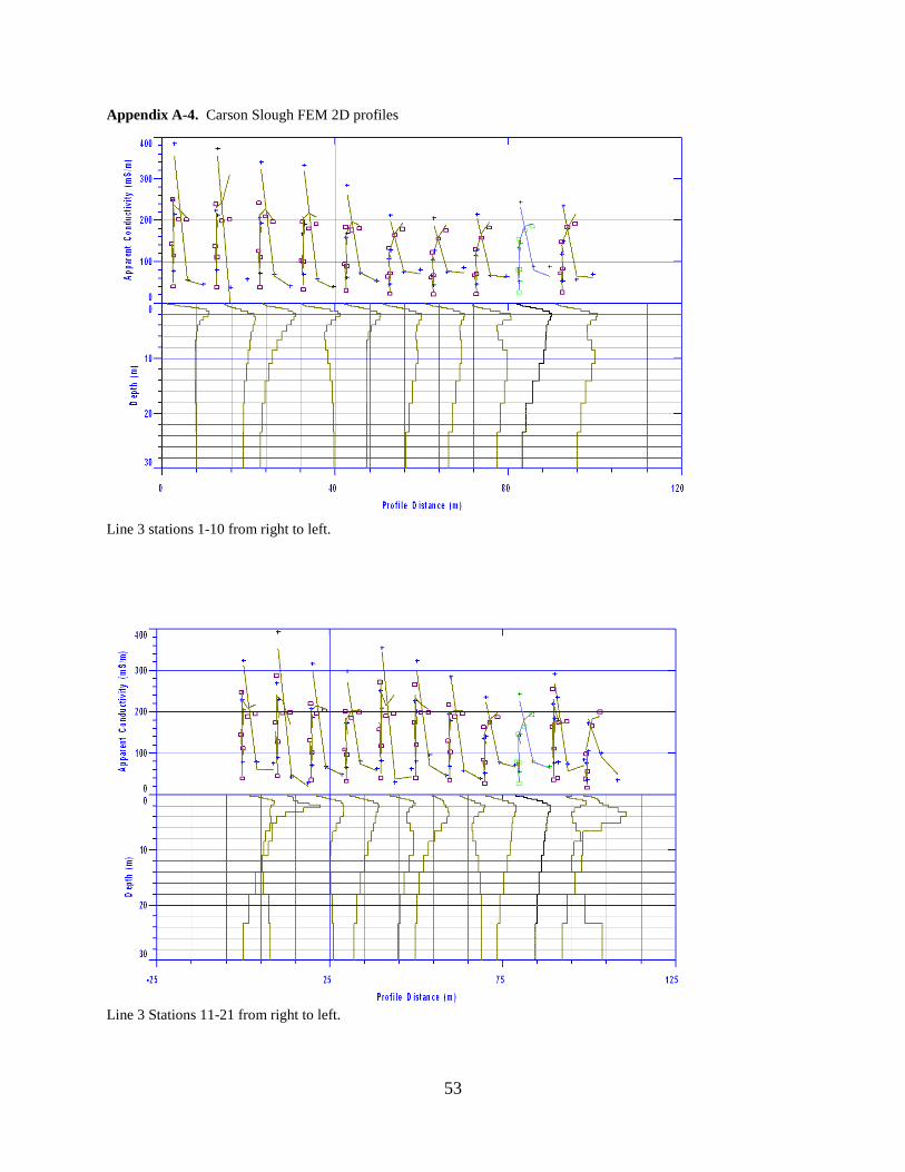
53

Appendix A-4. Carson Slough FEM 2D profiles

Line 3 stations 1-10 from right to left.

Line 3 Stations 11-21 from right to left.

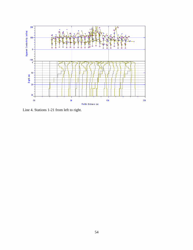
54

Line 4. Stations 1-21 from left to right.