Analysis of Drilled-Shaft Foundations for Overhead-Sign...
188
- \0 00 N I. CTR 3-5-78-244- ANALYSIS OF DRILLED-SHAFT FOUNDATIONS FOR OVERHEAD-SIGN STRUCTURES Gerald Lowe and Lymon C. Reese RESEARCH REPORT 244-2F PROJECT 3-5-78-244 CENTER FOR TRANSPORTATION RESEARCH BUREAU OF ENGINEERING RESEARCH THE UNIVERSITY OF TEXAS AT AUSTIN APRIL 1982
Transcript of Analysis of Drilled-Shaft Foundations for Overhead-Sign...

-\0 00 N
I.
CTR 3-5-78-244-
ANALYSIS OF DRILLED-SHAFT FOUNDATIONS FOR OVERHEAD-SIGN STRUCTURES
Gerald Lowe and Lymon C. Reese
RESEARCH REPORT 244-2F
PROJECT 3-5-78-244
CENTER FOR TRANSPORTATION RESEARCH BUREAU OF ENGINEERING RESEARCH
THE UNIVERSITY OF TEXAS AT AUSTIN
APRIL 1982
PARTIAL LIST OF REPORTS PUBLISHED BY THE CENTER FOR TRANSPORTATION RESEARCH
This list includes some of the reports published by the Center for Transportation Research and the organizations which were merged to form it: the Center for Highway Research and the Council for Advanced Transportation Studies. Questions about the Center and the availability and costs of specific reports should be addressed to: Director; Center for Transportation Research; ECJ 2.5; The University of Texas at Austin; Austin, Texas 78712.
7-1
7-2F
16-IF 23-1
23-2
23-3F
29-2F
114-4
114-5
114-6
114-7
114-8 114-9F 118-9F
123-30F
172-1 172-2F 176-4 176-5F 177-1
177-3
177-4
177-6
177-7
177-9
177-10
177-11
177-12
177-13
177-15
177-16 177"17 177-18
183-7
"Strength and Stiffness of Reinforced Concrete Rectangular Columns Under Biaxially Eccentric Thrust," by J. A. Desai and R. W. Furlong, January 1976. "Strength and Stiffness of Reinforced Concrete Columns Under Biaxial Bending," by V. Mavichak and R. W. Furlong, November 1976. "Oil, Grease, and Other Pollutants in Highway Runoff," by Bruce Wiland and Joseph F. Malina, Jr. , September 1976. "Prediction of Temperature and Stresses in Highway Bridges by a Numerical Procedure Using Daily Weather Reports," by Thaksin Thepchatri, C. Philip Johnson, and Hudson Matlock, February 1977 . "Analytical and Experimental Investigation of the Thermal Response of Highway Bridges," by Kenneth M. Will, C. Philip Johnson, and Hudson Matlock, February 1977. "Temperature Induced Stresses in Highway Bridges by Finite Element Analysis and Field Tests," by Atalay Yargicoglu and C. Philip Johnson, July 1978. "Strength and Behavior of Anchor Bolts Embedded Near Edges of Concrete Piers," by G . B. Hasselwander, J. 0. Jirsa, J. E. Breen, and K. Lo, May 1977. "Durability, Strength, and Method of Application of Polymer-Impregnated Concrete for Slabs," by Piti Yimprasert, David W. Fowler, and Donald R. Paul, January 1976. "Partial Polymer Impregnation of Center Point Road Bridge," by Ronald Webster, David W. Fowler, and Donald R. Paul, January 1976. "Behavior of Post-Tensioned Polymer-Impregnated Concrete Beams," by Ekasit Limsuwan, David W. Fowler, Ned H . Burns, and Donald R. Paul, June 1978. "An Investigation of the Use of Polymer-Concrete Overlays for Bridge Decks," by Huey-Tsann Hsu, David W. Fowler, Mickey Miller, and Donald R. Paul, March 1979. "Polymer Concrete Repair of Bridge Decks," by David W. Fowler and Donald R. Paul, March 1979. "Concrete-Polymer Materials for Highway Applications," by David W. Fowler and Donald R. Paul, March 1979. "Observation of an Expansive Clay Under Controlled Conditions," by John B. Stevens, Paul N. Brotcke, Dewaine Bogard, and Hudson Matlock, November 1976. "Overview of Pavement Management Systems Developments in the State Department of Highways and Public Transportation," by W. Ronald Hudson, B. Frank McCullough, Jim Brown, Gerald Peck, and Robert L. Lytton, January 1976 (published jointly with the Texas State Department of Highways and Public Transportation and the Texas Transportation Institute, Texas A&M University). "Axial Tension Fatigue Strength of Anchor Bolts," by Franklin L. Fischer and Karl H. Frank, March 1977. "Fatigue of Anchor Bolts," by Karl H . Frank, July 1978. "Behavior of Axially Loaded Drilled Shafts in Clay-Shales," by Ravi P. Aurora and Lymon C. Reese, March 1976. "Design Procedures for Axially Loaded Drilled Shafts," by Gerardo W. Quiros and Lymon C. Reese, December 1977. "Drying Shrinkage and Temperature Drop Stresses in Jointed Reinforced Concrete Pavement," by Felipe Rivero-Vallejo and B. Frank McCullough, May 1976. "A Study of the Performance of the Mays Ride Meter," by Yi Chin Hu, Hugh J . Williamson, and B. Frank McCullough, January 1977. "Laboratory Study of the Effect of Nonuniform Foundation Support on Continuously Reinforced Concrete Pavements," by Enrique Jimenez, B. Frank McCullough, a:nd W. Ronald Hudson, August 1977 . "Sixteenth Year Progress Report on Experimental Continuously Reinforced Concrete Pavement in Walker County," by B. Frank McCullough and Thomas P. Chesney, April 1976. "Continuously Reinforced Concrete Pavement: Structural Performance and Design/ Construction Variables," by Pieter J. Strauss, B. Frank McCullough, and W. Ronald Hudson, May 1977. "CRCP-2, An Improved Computer Program for the Analysis of Continuously Reinforced Concrete Pavements," by James Ma and B. Frank McCullough, August 1977. "Development of Photographic Techniques for Performing Condition Surveys ," by Pieter Strauss, James Long, and B. Frank McCullough, May 1977. "A Sensitivity Analysis of Rigid Pavement Overlay Design Procedure," by B. C . Nayak, W. Ronald Hudson, and B. Frank McCullough, June 1977. "A Study of CRCP Performance: New Construction Vs. Overlay," by James I. Daniel, W. Ronald Hudson, and B. Frank McCullough, April 1978. "A Rigid Pavement Overlay Design Procedure for Texas SDHPT," by Otto Schnitter, W. R. Hudson, and B. F. McCullough, May 1978. "Precast Repair of Continuously Reinforced Concrete Pavement," by Gary Eugene Elkins, B. Frank McCullough, and W. Ronald Hudson, May 1979. "Nomographs for the Design of CRCP Steel Reinforcement," by C. S. Noble, B. F. McCullough, and J. C. M. Ma, August 1979. "Limiting Criteria for the Design of CRCP," by B. Frank McCullough, J. C. M. Ma, and C. S. Noble, August 1979. "Detection of Voids Underneath Continuously Reinforced Concrete Pavements," by John W. Birkhoff and B. Frank McCullough, August 1979. "Permanent Deformation Characteristics of Asphalt Mixtures by Repeated-Load Indirect Tensile Test," by Joaquin Vallejo, Thomas W. Kennedy, and Ralph Haas, June 1976.
(Continued inside back cover)
1. Report No. 2. Government Accession No.
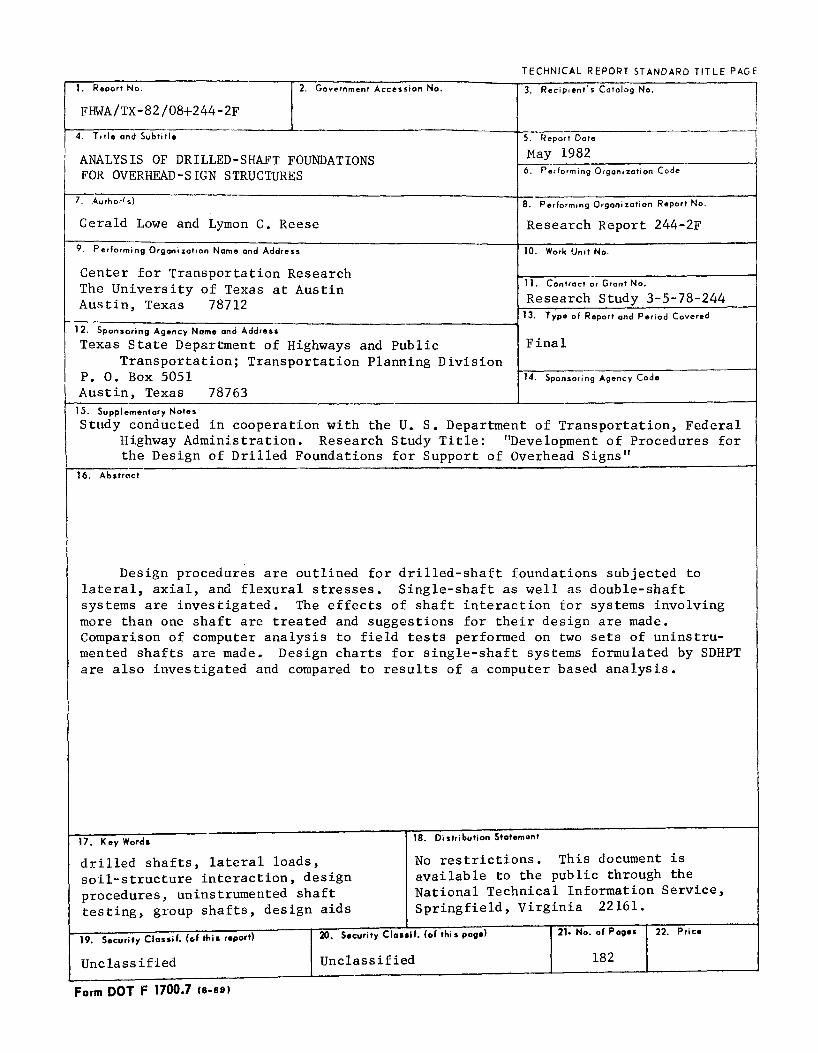
FHWA/TX-82/08+244-2F
4. T1tle and Subtitle
ANALYSIS OF DRILLED-SHAFT FOUNDATIONS FOR OVERHEAD-SIGN STRUCTURES
7. Authorls)
Gerald Lowe and Lyman C. Reese
9. Performing Organization Nome and Address
TECHNICAL REPORT STANDARD TITLE PACE
3. Recip1ent"s Catalog No.
5. Report Date
May 1982 6. Performing Organization Code
8. Perform1ng Organization Report No.
Research Report 244-2F
10. Work Unit No.
11. Contract or Grant No.
Research Study 3-5-78-244
Center for Transportation Research The University of Texas at Austin Austin, Texas 78712
13. Type of Report and Period Covered ~~~------------~~-----------------------------~ 12. Sponsoring Agency Name and Address
Texas State Department of Highways and Public Transportation; Transportation Planning Division
P. 0. Box 5051
Final
14. Sponsoring Agency Code
Austin, Texas 78763 15. Supplementary Nates
Study conducted in cooperation with the U. S. Department of Transportation, Federal Highway Administration. Research Study Title: "Development of Procedures for the Design of Drilled Foundations for Support of Overhead Signs"
r--,l,--6-. _A_b,_s-t-ra_c_t
Design procedures are outlined for drilled-shaft foundations subjected to lateral, axial, and flexural stresses. Single-shaft as well as double-shaft systems are investigated. The effects of shaft interaction for systems involving more than one shaft are treated and suggestions for their design are made. Comparison of computer analysis to field tests performed on two sets of uninstrumented shafts are made. Design charts for single-shaft systems formulated by SDHPT are also investigated and compared to results of a computer based analysis.
17. Key Wards
drilled shafts, lateral loads, soil-structure interaction, design procedures, uninstrumented shaft testing, group shafts, design aids
18. Di stributian Statement
No restrictions. This document is available to the public through the National Technical Information Service, Springfield, Virginia 22161.
19. Security Classif. (of this report) 20. Security Claulf. (of this page) 21. No. of Pages 22. Price
Unclassified Unclassified 182
Form DOT F 1700.7 cs-s9l

!!!!!!!!!!!!!!!!!!!"#$%!&'()!*)&+',)%!'-!$-.)-.$/-'++0!1+'-2!&'()!$-!.#)!/*$($-'+3!
44!5"6!7$1*'*0!8$($.$9'.$/-!")':!

ANALYSIS OF DRILLED-SHAFT FOUNDATIONS FOR OVERHEAD-SIGN STRUCTURES
by
Gerald Lowe Lyman C. Reese
Research Report Number 244-2F
Development of Procedures for the Design of Drilled Foundations for Support of Overhead Signs
Research Project 3-5-78-244
conducted for
Texas State Department of Highways and Public Transportation
in cooperation with the U.S. Department of Transportation
Federal Highway Administration
by the
CENTER FOR TRANSPORTATION RESEARCH
BUREAU OF ENGINEERING RESEARCH
THE UNIVERSITY OF TEXAS AT AUSTIN
May 1982

The contents of this report reflect the vie\vS of the authors, who are responsible for the facts and the accuracy of the data presented herein. The contents do not necessarily reflect the official views or poli~ies of the Federal Highway Administration. This report does not constitute a standard, specification, or regulation.
There was no invention or discovery conceived or first actually reduced to practice in the course of or under this contract, including any art, method, process, machine, manufacture, design or composition of matter, or any new and useful improvement thereof, or any variety of plant which is or may be patentable under the patent laws of the United States of America or any foreign country.
ii

PREFACE
This is the second of two reports for Research Project 3-5-78-244.
Presented in this report are design procedures for drilled shafts to be
used for the foundation of Overhead Sign Bridges. Summaries of procedures for
the design of single shafts in tension and compression are made as well as
suggested procedures for shafts subjected to axial and lateral loads in con
junction with flexural loadings. The design of closely spaced shafts is also
summarized and their interaction evaluated. Results of field tests conducted
in San Antonio are also presented.
The authors would like to thank several individuals for their assistance,
both in the field and in the office. Mssrs. Maltsberger and Hoy of SDHPT as
well as Mr. Hank Franklin and Mr. Jim Anagnos contributed greatly to the field
test efforts. Lola Williams and Cathy Collins provided support in the office
for both field testing and manuscript preparation. Charles Covill, as
engineer-representative of SDHPT, also made suggestions and offered many hours
of help.
The authors would also like to acknowledge the generous support of the
Federal Highway Administration.
May 1982
iii
Gerald F. Lowe
Lymon C. Reese

!!!!!!!!!!!!!!!!!!!"#$%!&'()!*)&+',)%!'-!$-.)-.$/-'++0!1+'-2!&'()!$-!.#)!/*$($-'+3!
44!5"6!7$1*'*0!8$($.$9'.$/-!")':!

ABSTRACT
Design procedures are outlined for drilled-shaft foundations subjected to
lateral, axial, and flexural stresses. Single-shaft as well as double-shaft
systems are investigated. The effects of shaft interaction for systems
involving more than one shaft are treated and suggestions for their design are
made. Comparison of computer analysis to field tests performed on two sets of
uninstrumented shafts are made. Design charts for single-shaft systems formu
lated by SDHPT are also investigated and compared to results of a computer
based analysis.
KEY WORDS: drilled shafts, lateral loads, soil-structure interaction, design
procedures, uninstrumented shaft testing, group shafts, design aids
v

!!!!!!!!!!!!!!!!!!!"#$%!&'()!*)&+',)%!'-!$-.)-.$/-'++0!1+'-2!&'()!$-!.#)!/*$($-'+3!
44!5"6!7$1*'*0!8$($.$9'.$/-!")':!

SU}U1ARY
This study concerns the design of drilled-shaft foundations for use with
Overhead Sign Bridges. Design procedures for single- and double-shaft systems
were presented with attention given to the effects of soil-structure and
structure-structure interaction. Design charts formulated by SDHPT were
checked and found to be adequate for design within stated conditions.
Alternate methods of design for unusual cases were advanced for both single
and double-shaft systems.
The results of two field tests on uninstrumented shafts were presented
and comparisons to predicted results were made. The observed results indi
cated that the computer-based analysis gave conservative results.
vii

!!!!!!!!!!!!!!!!!!!"#$%!&'()!*)&+',)%!'-!$-.)-.$/-'++0!1+'-2!&'()!$-!.#)!/*$($-'+3!
44!5"6!7$1*'*0!8$($.$9'.$/-!")':!
IMPLEMENTATION STATEMENT
This study presents design procedures for foundations of Overhead Sign
Bridges. A procedure for design by charts as well as a computer-based
procedure are presented, with the appropriate method of design to be selected
on the basis of site information that is available.
Where reliable and adequate data are available, the computer-based method
should be used. When only a limited amount of information can be obtained,
the procedure utilizing the charts should be followed.
It is suggested that, conditions permitting, double-shaft systems be
replaced by adequately designed single-shaft systems. Thus, a more efficient
system will be attained.
ix

!!!!!!!!!!!!!!!!!!!"#$%!&'()!*)&+',)%!'-!$-.)-.$/-'++0!1+'-2!&'()!$-!.#)!/*$($-'+3!
44!5"6!7$1*'*0!8$($.$9'.$/-!")':!
TABLE OF CONTENTS
PREFACE • . . . . . . . . . . . . . iii
ABSTRACT . . . . . . . . . . . . . . . v
SUMMARY . vii
IMPLEMENTATION STATEMENT ix
LIST OF TABLES . . . . . . . . . . . . . . XV
LIST OF FIGURES •• xvii
LIST OF SYMBOLS
CHAPTER 1. INTRODUCTION
Overhead-Sign System Us age • • • • • • • • • • • • • • • Superstructure Configurations Foundation Configuration
Available Methods of Analysis and Design • Analysis • • • • • • • • •• Design •••••••••• Benefits of Improved Methods of Analysis and Design
CHAPTER 2. ANALYSIS AND DESIGN OF SINGLE-SHAFT SYSTEM
Analytical Methods ••••.•••• System Configuration .•... Available Methods of Analysis • Application of Analytical Methods
SDHPT Design . • • • • • • ••• SDHPT Design Aids • •
to the Design Process
Description • • • • • • Failure Criteria for SDHPT Design Aids • Design Example Using SDHPT Design Aid Analysis Using COM623 • • • • • • • • • Formulation of Data Set for Computer Solution Variation of Parameters Used in Computer Solution Effects of Parameter Variation on Shaft Behavior ••••
Comparison of Computer Solution to Design-Aid Solution •••.•
xi
xxi
1 1 1 4 4 4 4 5
7 7 9 9
10 10 10 10 14 16 16 17 17 24
xii
CHAPTER 3. ANALYSIS AND DESIGN OF DOUBLE-SHAFT SYSTEMS
Application of Load •••. o o o o o o o o o o •
Analysis of a Shaft Subjected to Tensile Loading Cohesive Soils o o ••• o o o o o o 0 o •
Cohesionless Soils .•• o o
Analysis of a Shaft Subjected to a Compressive Loading Cohesive Soils o • o • o o o o o o • o o
Cohesionless Soils o o o o o o o o o •
Additional Factors Affecting Shaft Capacity Available Programs for Computer Assisted
Analysis of Shafts in Compression . Design of Closely Spaced Shafts o o o o o o
Interaction of Closely Spaced Shafts Under Lateral Loads . • o o o o • • o
Proposed Methods of Analysis . o o • o o
Application of Analytical Method to Design Example Problem o o o o o o • • o o o • • • •
Interaction of Closely Spaced Shafts Under Axial Load
Axial Deflection Shaft Capacities
CHAPTER 4. DESIGN PROCEDURE USING COMPUTER-BASED METHODS OF ANALYSIS
Present Capabilities . o • o o o o o • o o o •
Computer-Based Analysis o o o o o o • o o o
Application of Analytical Methods to Design Suggested Design Procedure • o o o
Example Problem o • • • • • o • • • o o o
Comparison of Computer-Based Design and Chart Design
CHAPTER 5. GENERATION OF DESIGN AIDS
Generation Procedure . o o o •••• o • o • o o
Establishment of Range of Tables and Curves o
Generation of Curves . o o o o • • o
Use of Tables and Curves o o • o o o o o o
CHAPTER 6. SAN ANTONIO TEST AND RESULTS
Test Site and Conditions Test Details . o o o o o
Shaft Configuration Load S ys tern . o o o o
System for Measuring Deflection o o o o o o
Loading and Results of Field Test o o o o o o
Comparison of Field Test Results to Computer Analyses o
Conclusions o o • o • o o o o o o o o o o o o o o o o o o o o o
27 27 28 35 37 37 42 45
46 46
46 48 50 52
61 61 64
67 67 68 68 69 76
81 82 82 86
87 88 88 93 95 95 97
103

CHAPTER 7. COMPARISON OF SINGLE AND DOUBLE SHAFT SYSTEMS
Economic Comparison of Proposed Designs ••..•••• Additional Factors Affecting Selection of Foundation Type
CHAPTER 8. CONCLUSIONS
Design Concepts .••••••••••.•••• Two-Shaft System • • •• Single-Shaft System • • •••
Design Procedures • • • • • ••• Use of Charts in Design ••••• Use of Computer Program in Design (COM623)
Factors of Safety and Cost Comparisons Factors of Safety • • • • • . . . . . Cost Comparison .••.••••.•••
San Antonio Field Test •
REFERENCES
APPENDIX
Test Results Further Research
. . . .
xiii
105 107
109 109 109 109 109 110 110 110 110 110 110 111
113
117

!!!!!!!!!!!!!!!!!!!"#$%!&'()!*)&+',)%!'-!$-.)-.$/-'++0!1+'-2!&'()!$-!.#)!/*$($-'+3!
44!5"6!7$1*'*0!8$($.$9'.$/-!")':!

Table
2.1
3.1
3.2
3.3
3.4
3.5
3.6
7.1
A.l
LIST OF TABLES
Summary of Shaft Design Using SDHPT Design Charts
Correlation Between Blow Count from Penetration Tests and Undrained Shear Strength ••••
Design Parameters for Drilled Shafts in Clay
Design Parameters for Base Resistance for Drilled Shafts in Clay .• o o o
Design Parameters for Drilled Shafts in Clay-Shale
Tip Movement Factor, kf
Design Parameters for Drilled Shafts in Sand
Comparison of Single- and Double-Shaft Systems
Detailed Input Guide with Definitions of Variables
XV
Page
15
34
39
41
43
43
44
106
127

!!!!!!!!!!!!!!!!!!!"#$%!&'()!*)&+',)%!'-!$-.)-.$/-'++0!1+'-2!&'()!$-!.#)!/*$($-'+3!
44!5"6!7$1*'*0!8$($.$9'.$/-!")':!

Figure
1.1
2.1
2.2
2.3
2.4
2.5
2.6
2.7
LIST OF FIGURES
Typical configuration of an overhead-sign structure •
Loadings and soil reactions on a shaft
Failure limits used in the generation of SDHPT design charts
Column moment selection. Texas SDHPT Design Chart
Sheet OSBC-SC-Z4,
Drilled shaft moment selection and drilled shaft or column reinforcement selection. Sheet OSBS-SC, Texas SDHPT Design Charts • • • • • • • . •••••
Sheet OSB-FD-SC. SDHPT Design Charts
Deflected shapes - rigid and flexible behavior
Shaft embedment length versus groundline deflection -variations in loading ••••••••••••••••
2.8 Groundline deflection versus lateral load -load and length variations
2.9 Groundline deflection versus lateral load -variations in shaft moment of inertia
3.1
3.2
3.3
and unit weight of soil ••••••
Correlation factor, of shafts in tension
a , for design
Breakout factor, F , for clay soils . c
Breakout factor, F q
for sand soils •
3.4 Effective shaft length, t , for shafts
3.5
3.6
with underreams
Ultimate side resistance, of shafts in tension
f u
for design
Shaft capacity versus embedment length . . .•••••••••
xvii
Page
2
8
8
11
12
13
19
20
22
23
29
31
32
33
36
47
xviii
Figure
3.7
3.8
3.9
3.10
3.11
3.12
3.13
3.14
4.1
4.2
4.3
4.4
4.5
5.1
5.2
5.3
6.1
6.2a
6.2b
6.3
6.4
6.5
6.6
6.7
Double-shaft group example problems •
Influence factor I for fixed-head piles • PF
Interaction factors a for fixed-head piles pf
Selection of p-y curve modifier
Equivalent shaft deflections and moments for example problem for double-shaft group
Influence factor I 1 for axial displacement •••••••••
Interaction a1 for axial displacement .
Free body of two-shaft system .
Parameters for design of single shaft •
Shaft moment versus lateral load
Groundline deflection versus lateral load • . . . . . Groundline deflection versus embedment length of shaft . . . • • • • • • • • • • .
Bending moment in shaft versus depth
Tables of ultimate moment . . • • • •
Groundline deflection versus shaft moment
Groundline deflection versus shaft length •
San Antonio test site . . . . . . . . . . . . ' . . . . . . . . San Antonio test site 1 •
San Antonio test site 2 .
Soils test results
Load system configuration .••••••••
Deflection and slope measurement system configuration .••••
Lateral load versus groundline deflection •
Lateral load versus groundline deflection •
Page
53
55
57
59
60
62
62
65
70
72
74
75
77
83
84
85
89
90
91
92
94
96
98
99

Figure
6.8
6.9
6.10
A.l
Ao2
A.3
A.4
A.5
A.6
Lateral load versus groundline deflection •
San Antonio test, observed failure patterns .
San A~tonio test, computer analyses and field test results •.••••••
Portion of a beam subjected to bending
Beam cross section for example problem
Stress-strain curve for concrete used by Program PMEI . • . .
Stress-strain curve for steel used by Program PMEI o o o •
Data input form for computer program PMEI • .
Concrete column cross-sections for example problems .
xix
Page
100
101
102
119
119
124
124
126
128

!!!!!!!!!!!!!!!!!!!"#$%!&'()!*)&+',)%!'-!$-.)-.$/-'++0!1+'-2!&'()!$-!.#)!/*$($-'+3!
44!5"6!7$1*'*0!8$($.$9'.$/-!")':!

LIST OF SYMBOLS
TBA average shear stress on a freebody due to load QA
p
s
axial deflection of pile
correlation factor
deflection of a single pile calculated by
deflection of a single pile due to a unit
deflection of the kth pile
effective angle of internal friction
effective unit weight of soil
influence factor
influence factor
ratio of settlements
reduction factor
reinforcement ratio
relational angle between piles in a group
strain at 50 percent of failure
total axial displacement of shaft
unit weight of soil
unit weight of water
cross sectional area of shaft
area of shaft base
side area of shaft
xxi
elastic
load
methods

xxii
c circumference of shaft
undrained shear strength of clay or shale
D
d u
EI
E c
E s
F c
F q
f
f I c
f u
f y
H
HT
H avg
H. J
Hk
H m
diameter of shaft
diameter of shaft bell
depth at which f occurs u
flexural stiffness
modulus of elasticity of concrete
soil modulus
breakout factor for clay
breakout factor for sand
side friction
concrete compression strength
ultimate side resistance
yield stress of reinforcing steel
total depth of embedment of shaft
total lateral load on pile group
average lateral load on pile in a
load the .th pile on J
load the th
pile on k
load the th pile on m
11
an influence factor
I gross moment of inertia gr
group
I moment of inertia '\lith transfonned steel area tr
K lateral earth pressure coefficient
~ ratio of pile stiffness to soil stiffness

k s
1
1
M max
M n
m
N
N c
n
p u
p
pmax
Pu
QA
QBA
Qb
Qs
Qu
base movement factor
kips (1000 lbs)
modulus of subgrade reaction
shaft embedment length
effective shaft length
maximum shaft moment
nominal moment
moment at shaft head
design moment
number of piles in the group
blow count SPT or SDHPT-THD Penetrometer Test
bearing capacity factor
number of cycles for cyclic loading case
lateral load at shaft head
allowable lateral load on shaft
ultimate uplift capacity of shaft
axial load
correlation factor
soil reaction
effective overburden pressure
maximum allowable soil reaction
ultimate soil reaction
load on pile A
load induced on pile B due to QA
capacity of shaft in end bearing
capacity of shaft due in skin friction
uplift capacity of shaft underream
xxiii
xxiv
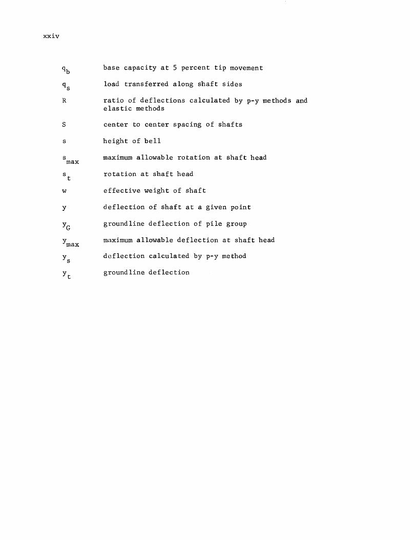
R
s
s
s max
w
y
base capacity at 5 percent tip movement
load transferred along shaft sides
ratio of deflections calculated by p-y methods and elastic methods
center to center spacing of shafts
height of bell
maximum allowable rotation at shaft head
rotation at shaft head
effective weight of shaft
deflection of shaft at a given point
groundline deflection of pile group
maximum allowable deflection at shaft head
deflection calculated by p-y method
groundline deflection

CHAPTER 1. INTRODUCTION
OVERHEAD-SIGN SYSTEM
USAGE
Since the inception of the Federal Interstate Highway System in the
1950's, the number of miles of divided, multi-lane, limited access roadway in
use has continued to increase yearly. One need that arose with this highway
system was for a sign system that is easily legible and understandable to the
motorist, and the development of the overhead sign has provided an acceptable
solution to this problem. Spanning the full width of the roadway, this system
quickly provides directional information in an unambiguous form; the proper
lane for a given destination can be easily marked overhead. The structural
problem of the sign support has been solved by the use of steel trusses with
spans of up to 150 feet (45.7 m). The structure must carry the dead load of
the signs, lighting, and truss, as well as the live loadings from wind, snow,
and ice. The loads are transmitted through vertical support towers to the
foundation (Fig 1.1), which typically consists of one or more drilled shafts.
This paper presents methods of analysis and design for both single- and
double-shaft systems, and an economic comparison is made.
SUPERSTRUCTURE CONFIGURATIONS
There are currently three configurations for overhead-sign systems that
are used or proposed for use by the Texas State Department of Highways and
Public Transportation (SDHPT). The first and most commonly observed con
figuration consists of a horizontal truss supported by vertical trusses at
either end. The horizontal truss is a box-type structure consisting of planar
Pratt trusses fabricated from steel angles. All signs and lighting are bolted
to this structure. At either end of this horizontal structure, vertical
trusses, consisting of wide flanges for chords and angles for diagonal web
members, carry all loads to the foundation. These vertical trusses are
1

2
ELEVATION
~<t. Span with odd
I number of panels *' o" : sign Depth
=-= .... .::.._-:~ ~""7-t:' Span with even .1.____,,_~ _ 'm:~ number of ponels \~, C
I. ~;i
--- :J =~ 0~ E 0 -0
Highest Elevation of Roadway under Signs1 m
ELEVATION
A~,
t 7'-6" I
A <EJ
I() I (j) I() (j)
VI <.D v (j) <X <X <( <X II) II) II) II)
11)1 II) II) II) ::l ::l ::l ::l .= t!= .= .= .... '- .... ""' 0 0 0 0 LLLLLLLL
l For Truss A 45 _For Truss A 66 SECTION A- A
Fig 1.1. Typical configuration of an overhead-sign structure.
(1 ft = .3048 m)
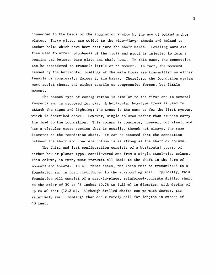
connected to the heads of the foundation shafts by the use of bolted anchor
plates. These plates are welded to the wide-flange chords and bolted to
anchor bolts which have been cast into the shaft heads. Leveling nuts are
then used to attain plumbness of the truss and grout is injected to form a
bearing pad between base plate and shaft head. In this case, the connection
can be considered to transmit little or no moment. In fact, the moments
caused by the horizontal loadings at the main truss are transmitted as either
tensile or compressive forces to the bases. Therefore, the foundation system
must resist shears and either tensile or compressive forces, but little
moment.
The second type of configuration is similar to the first one in several
respects and is proposed for use. A horizontal box-type truss is used to
attach the signs and lighting; the truss is the same as for the first system,
which is described above. However, single columns rather than trusses carry
the load to the foundation. This column is concrete, however, not steel, and
has a circular cross section that is usually, though not always, the same
diameter as the foundation shaft. It can be assumed that the connection
between the shaft and concrete column is as strong as the shaft or column.
The third and last configuration consists of a horizontal truss, of
either box or planar type, cantilevered out from a single steel-pipe column.
This column, in turn, must transmit all loads to the shaft in the form of
moments and shears. In all three cases, the loads must be transmitted to a
foundation and in turn distributed to the surrounding soil. Typically, this
foundation will consist of a cast-in-place, reinforced-concrete drilled shaft
on the order of 30 to 48 inches (0.76 to 1.22 m) in diameter, with depths of
up to 40 feet (12.2 m). Although drilled shafts can go much deeper, the
relatively small loadings that occur rarely call for lengths in excess of
40 feet.
3

4
FOUNDATION CONFIGURATION
Although three types of sign configurations exist, the design or analysis
of the foundations can be grouped into two main categories, i.e., single shaft
and double shaft. The double-shaft system is used in conjunction with the
first sign system that was discussed. In this system, each foundation shaft
must primarily resist axial forces of a compressive or tensile nature in com
bination with a horizontal component. Relatively speaking, shaft moments
caused by the horizontal shears are small.
For the laet two sign systems mentioned, the single-shaft-foundation
system is subjected to a slightly different loading condition. For the
structure with supports at each end, the vertical loads due to dead load as
well as the horizontal shears are practically the same as in the double-shaft
system. However, the moments produced by the horizontal loads are no longer
transmitted as axial forces; they are transmitted to the shafts as moments and
must be resisted by the shafts in bending. The cantilever-type structure is
subjected to torsion along with shear and moment. The cantilever design will
not be discussed in this report.
AVAILABLE METHODS OF ANALYSIS AND DESIGN
ANALYSIS
The processes of analysis and design of systems using drilled shaft
foundations are continually being refined. Newer and more capable methods of
computation have allowed the use of systems of analysis and design heretofore
unavailable. A problem can now be solved not only by the use of differential
equations but also by the use of non-dimensional coefficients or computer
based finite difference methods (Refs 5, 13, 15, and 17). The desired
accuracy of the model used for solution of the problem at hand will determine
which method of analysis is selected.
DESIGN
The use of computers has encouraged the development of simplified design
charts. While these charts are, of practical necessity, restrictive in their
application, they can be utilized by the engineer in everyday practice. Under
the proper circumstance they can be used for an adequate and quick solution to

a given problem. If the situation is too complex, the charts may still be
used to give an idea of an appropriate starting point for a computer-based
solution. Such computer··based solutions allow a higher degree of freedom in
modelling to match the complexities encountered in more difficult problems.
BENEFITS OF IMPROVED METHODS OF ANALYSIS AND DESIGN
5
Improved methods of analysis and design will in turn lead to the better
use of both :materials and manpower. A quick and accurate design of the system
will allow consideration of construction methods and site-related problems
that affect shaft capacities and will allow comparisons to be made with other
possible solutions. Situations in which single-shaft foundations may be used
in lieu of group shafts or piling, as well as situations in which double-shaft
or group systems will pe~form better than single-shaft systems, will be more
easily recognizable. Since not all situations are amenable to the single,
shaft solution, the appropriate use of an alternative system will be encour
aged by a rigorous investigation.
The ability to establish several different approaches quickly will allow
more time to be spent in the evaluation and comparison of economic and con
struction faetors pertinent to each solution. In many instances, the econom
ics will clearly indicate one solution over another, but in some instances the
choice may not be as obvious. Under these circumstances, th~ ability to per
form an accurate analysis and design is important and can lead to savings in
available funds. In addition, the funamentals that are outlined herein are
applicable, v7ithout modification, to the problems encountered in the analysis
and design of foundations for bent caps, abutments, retaining walls, and
similar structures.
The methods of analysis have been treated quite extensively in other
papers. The major thrust of this paper is to present design methods and
design aids; thus, little time will be spent on analysis other than for a
brief review of the existing methods.

!!!!!!!!!!!!!!!!!!!"#$%!&'()!*)&+',)%!'-!$-.)-.$/-'++0!1+'-2!&'()!$-!.#)!/*$($-'+3!
44!5"6!7$1*'*0!8$($.$9'.$/-!")':!

CHAPTER 2. ANALYSIS AND DESIGN OF SINGLE-SHAFT SYSTEM
ANALYTICAL METHODS
Before a logical procedure for design can be formulated, a rational
method of analysis must be established. Through the use of simplifying
assumptions, the problem must be reduced to such a state that a manageable
mathematical model can be constructed. Once this is accomplished, the desired
design procedure can be established, with the understanding that the solution
will never be "exact." Although such a design solution may not be theoreti
cally correct, it may be close enough to real life phenomena to be acceptable.
In essence, the solution of the problem that is presented herein reduces to
insuring that the soil can provide sufficient reaction to the shaft and that
the shaft itself will not fail while keeping the design economically viable.
SYSTEM CONFIGURA,lON ,,
The loadings\on the foundation system can be reduced to lateral load, , .. ~
axial load, and mom,ent, all applied at the pile head. The application of
these loads, single or in various combinations, will result in the establish
ment in the soil system of a reaction which, in turn, produces additional load
on the shaft (Fig 2.1). The shaft can be idealized as acting as a beam under
concentrated ~ dj.stributed loads, and the governing differential equations
of beam theory can be used for a solution of the problem. If the scheme shown
in Fig 2.1 is sufficiently simplified, a closed-form solution can be made.
Non-dimensional-coefficient solutions can be used if a more generalized scheme
is desired. The greatest degree of freedom, however, is offered by the use of
a computer solution using the finite difference method for the approximate
solution of the governing differential equations (Ref 13).
The foundation of the cantilever-type structure is also subjected to torsion but, as noted earlier, the cantilever design will not be treated in detail in this report.
7

8
Px I r ~Mt
---·•Pt
p
Fig 2.1. Loadings and soil reactions on a shaft.
Maximum Groundline
Deflection = 3 inches ( 7.6 em)
Fig 2.2. Failure limits used in the generation of SDHPT design charts.
9
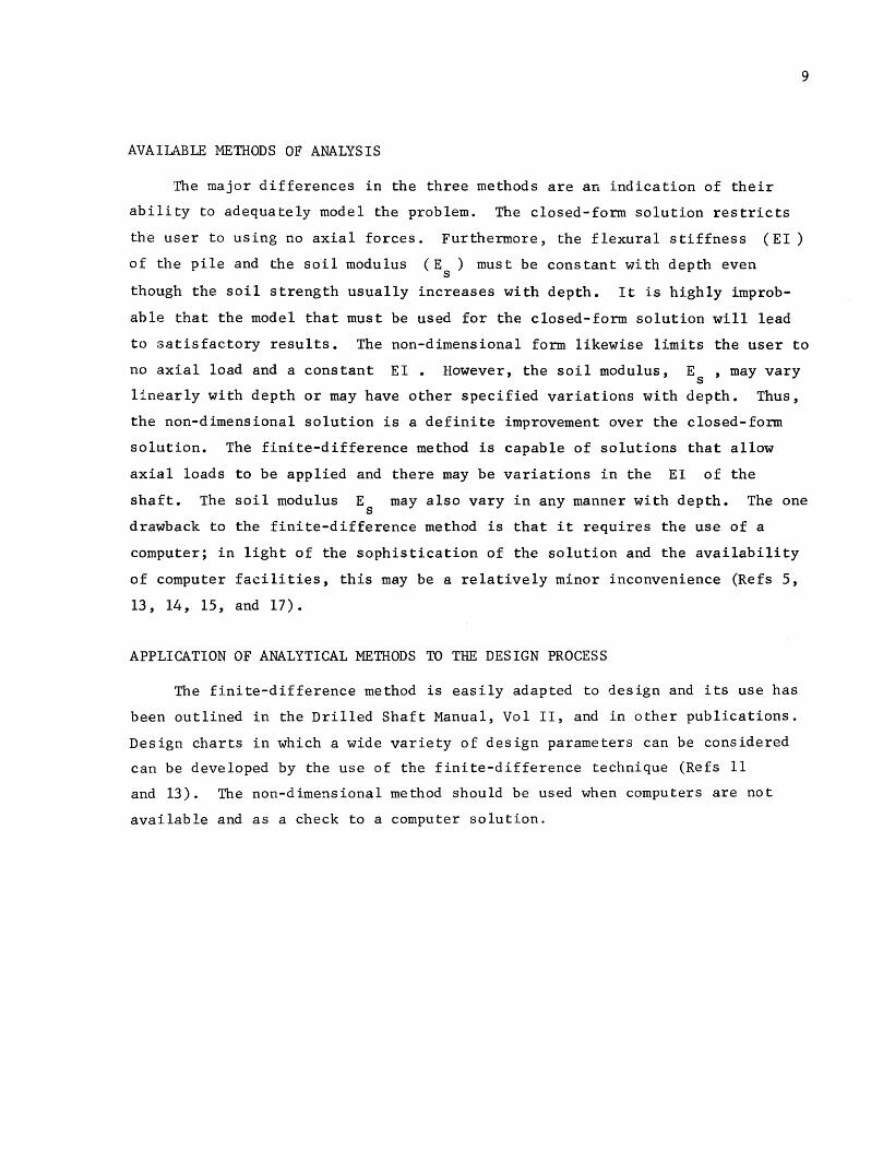
AVAilABLE METHODS OF ANALYSIS
The major differences in the three methods are an indication of their
ability to adequately model the problem. The closed-form solution restricts
the user to using no axial forces. Furthermore, the flexural stiffness (EI)
of the pile and the soil modulus ( E ) must be constant with depth even s
though the soil strength usually increases with depth. It is highly improb
able that the model that must be used for the closed-form solution will lead
to satisfactory results. The non-dimensional form likewise limits the user to
no axial load and a constant EI • However, the soil modulus, Es , may vary
linearly with depth or may have other specified variations with depth. Thus,
the non-dimensional solution is a definite improvement over the closed-form
solution. The finite-difference method is capable of solutions that allow
axial loads to be applied and there may be variations in the EI of the
shaft. The soil modulus E may also vary in any manner with depth. The one s
drawback to the finite-difference method is that it requires the use of a
computer; in light of the sophistication of the solution and the availability
of computer facilities, this may be a relatively minor inconvenience (Refs 5,
13, 14, 15, and 17).
APPLICATION OF ANALYTICAL METHODS TO THE DESIGN PROCESS
The finite-difference method is easily adapted to design and its use has
been outlined in the Drilled Shaft Manual, Vol II, and in other publications.
Design charts in which a wide variety of design parameters can be considered
can be developed by the use of the finite-difference technique (Refs 11
and 13). The non-dimensional method should be used when computers are not
available and as a check to a computer solution.
10
SDHPT DESIGN
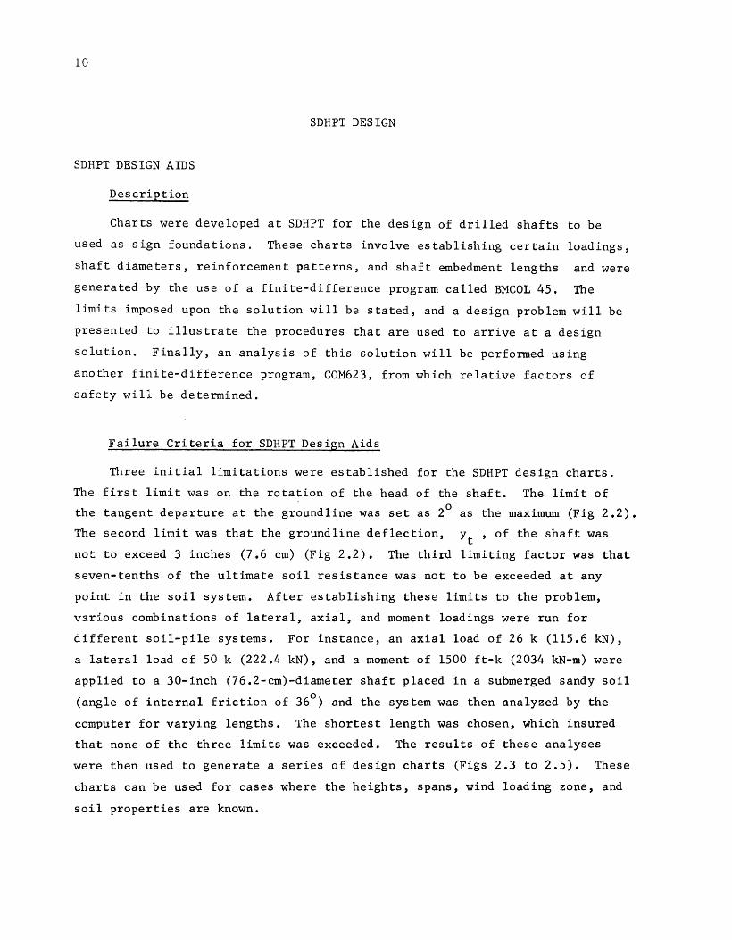
SDHPT DESIGN AIDS
Description
Charts were developed at SDHPT for the design of drilled shafts to be
used as sign foundations. These charts involve establishing certain loadings,
shaft diameters, reinforcement patterns, and shaft embedment lengths and were
generated by the use of a finite-difference program called BMCOL 45. The
limits imposed upon the solution will be stated, and a design problem will be
presented to illustrate the procedures that are used to arrive at a design
solution. Finally, an analysis of this solution will be performed using
another finite-difference program, COM623, from which relative factors of
safety wil1 be determined.
Failure Criteria for SDHPT Design Aids
Three initial limitations were established for the SDHPT design charts.
The first limit was on the rotation of the head of the shaft. The limit of
the tangent departure at the groundline was set as 2° as the maximum (Fig 2.2).
The second limit was that the groundline deflection, yt , of the shaft was
not to exceed 3 inches (7.6 em) (Fig 2.2). The third limiting factor was that
seven-tenths of the ultimate soil resistance was not to be exceeded at any
point in the soil system. After establishing these limits to the problem,
various combinations of lateral, axial, and moment loadings were run for
different soil-pile systems. For instance, an axial load of 26 k (115.6 kN),
a lateral load of 50 k (222.4 kN), and a moment of 1500 ft-k (2034 kN-m) were
applied to a 30-inch (76.2-cm)-diameter shaft placed in a submerged sandy soil
(angle of internal friction of 36°) and the system was then analyzed by the
computer for varying lengths. The shortest length was chosen, which insured
that none of the three limits was exceeded. The results of these analyses
were then used to generate a series of design charts (Figs 2.3 to 2.5). These
charts can be used for cases where the heights, spans, wind loading zone, and
soil properties are known.

ZONE 4 70 M.P.H. WIND [SPAN! REACT!ON8 I -COLUMN BENOJNG MOMENTS (FT. KIPS)
Ft. I O.L I W. L. 1Tor~j_j~'_l_l€' rl7 1-l 18' }191 J 20' l 21' J 22 ' Jg3' ]24' L?_e>' I 26' I 27 ' I 28' I 29'J3QJJ ~___l_]_~_jg_ht T!40,265l5 .03~g7 ' 8ij86j9 1 I96IIO I 10€ 112117122127132137142147 l53I15E 163168 !73
~ l !45 · :.. .98 5 .66 10.09 91 9? i02 10 8 114 !20 12€ ! 3 1 137 143 !49 154 160 166 1721 : 78 183 18S 195
61 I 50 13:3 3 I 6 . 2 9 I I . 2 ! I 0 I t ; c: 1'1 4 i 12 8 I~~- I 3 ~ _I 4 () ' 4 6 I 52 I ~~- ; 6 ~ I 7 2 i 7 8 ! 8 4 I 9 I I 9 7 2 0 .q 2 I 0 2 I 7 aJt' ~5~3 . 81 ! C 9 3,: :::.. 3L: .•• ; l !l 6tt2:: . !33 1t40 147 i 5 4 ! 61 , 168· i 75 ;E.;;:. 189 1~6 1203 21Cj2;7 224 231 2391
13 16014.15 1: :. ~ - ~ 346 ! 22j_I2 Sl~37 !~5 152 IE~-41-76 183 !91 199 2 0 _6 2 14 222 230 l2 73 24~ . 25 3 2€ 1 5' 6o l 4.55 e .2t 14.58 132 !4 0 1148 157 165 t74ft82jt? o 199 201 216 2 24 232 24 ! 249125 7 1 2. 66 2 74 283
~ 70 5.0S. 8.85 1!5.7 . 142 ! 5 i t60 169 178 i87J196 2J5 2_~ 2? 3 232 2 41 250 259 268l ~?..!--t_28 7 296 305 .. rf"l 75 s 4£: 9.4 ~ 1 G. e 3 I5 2 16 2 2 2 1s 1 1 9 . 1 2 c- 1 1 ;:; : : : 2 2 c 2 3 o 2 3 9 2 ~ 9 2 59 2 6 9 2 7 s 2 a 6 1 2 ~ s 1 3 G 7 ; 3 1 7 3 2 7 I
-..:..~ 80 6.0 2 927 i8 .06 !59! ! S9 1 ~ 7~J_i_g9IIC1~ ! 20S~. -~Q240 250 260 270 28_9_2 90 30(' ~ 3 ! ·:' 1~20 !3 3\'::_Ji.Q_ x w as 6 6 : I o. 5! 1 s. 19 ; 1 6 9 1 1 s c: 1 1 s · I 2 o 1 12 l :: f::::. 3 1 ;: 3 ~ ~: 4~ i 2 s ~ 2. 6 6 2 1 e i 2 a 7 !2 9 f: 1 :so s 3 1 9 3 3 ol3-zi 1· 3 s 2: 3 6 2 i z. '!' m so 7.03 1! .15 20.32 ISC l __ t9 :-T2o2 2141225i~~ili4 BJ ~~~91271 __?~2 293 305 316 327 33? 3:iot36rt373 384 I ~ on~ 9: 7.55 · II79 :2i. 45 !9 C. 2::(j~~J~2§..._?~c ! 25C!1_g~_74128629f· I::IG :322 33~ ! 3 4 5 : 358 ::. 7(' j 38 ; !3~~ 406j :;
C:t!OO 8 .2(; 12 .61 l£~ 3 .65 . ?07 22 ~ j233 1 ~' 461259!272l2B5 298 3 l i 324 337 1_3 50 1363 1 ~7_§J390 4C3 'tit.- i 429 4421 8 ~ I 0 5 8 . 9 I 1 3. 4 8 ! c: 4. 83 2 I 7 2 3 I . 2 4 5 2 59 2 7 2 2 8 6 12 99 3 14 3 2 7 3 ~ I 3 55 3 6 9 3 6 2 3 9 € i 4 I 0 I 4 2 ::. I .c, 3 7 j4 5 : I 4 6 5 ... m!, :o 9 .34 t4.15 26.02'228 2_±2_f-~~U27t 286 3oo~~J5 329 34W5e 372j3 E7 401 4l6143 C. I445 !45~; j•P'3 _;4ssl ~
I 115 9.87 14.81 2720'239.?5.5 ~~2.8412 991314 ji_<9I344j360 !3 75 13 so j ·, o·:·. 4 zc j <35 i <so 146: 14 gc ' 4 95! :> 11 I ~ , 120 . '0.45115 .52 . ::9.82 ' :: S i _1 ?S_ ~ b3l2~9~~331 r} 4.§J~£.L3 '8, 394!410_ ... ~-~ 45·;r ·47 3 ! 48 95051?.2' 15-3f ;
i !2~ . 3C ' I€.2C -: . ; o ~; ':?C~ j ;:::· ·.: l(:~ · :. . : 3i2 j3281 :: 4 5 i 3C:.I 37i~.:>?2J_~ ! ; 42£!~4 -q ,:; 51 ~ 477 49-:: j : .~ : ' '2 7 ~ 54 Ji 5 SG ~ i-:- 'l j ! :~0':", ~ _-r~-; :- 7.- - ~::-::, --::;- :.:- ~~ ;:;-;,~~:-:-:;-? C l . ~? 1 c-:-l-r:-T;-c.·~- -~ -~ -_;.-, ~~- ~ .': --;:;:- --Q l "-. I I C:: ., 1 --;-;; . ~ .. {... • 5 8 3 :
6061 63 1
:~o
,-!· 561 ~ t 583 u
(I ft =.3048m, I lb-ft =1.356 N-m, lib =.4536 kg)
Fig 2.3. Column moment selection. Sheet OSBC-SC-Z4, Texas SDHPT Design Charts.
r-' r-'
COLUMN OR DRILLED SHAFT
DRILLED SHAFT MOMENTS RE INFORC ING STEEL IGR. 60i
CLAY SOIL
36"• DR. SHAFT 42" ' DR. SHAFT 30000
COLUMN OR SHAFT SIZE MOMENT
4
I
8
I
12
I
20 IB 10 20 30 50
8 i 12 T 20
20 I 30 I 50
~ • ' J I ' " I I I 1------ -~-- -- --'---------+- - - - -~---!.--i
- --+--- -- - ----r-- ---- -r---t-------1 I -- -·- ·-
56 4 548 54 3 53 7 ~--+==~-
__J_ 6 50 628 623 6 I 6 7 3 9 7 I 2 703 6 9 4 i 1 8 2 5 785 7-:' 3
909 , 87 5 I 863 ,~
~ I . .., .. .., I J VV --~ ~ ~"~ II 9 98 i 95~~4-~ --- -- - 1091 ! t ::J 43 i 027 1 1011
--'---='--+-----'-=--=-=~~~~L-1~ ~_Q~~ ~v ~1_U_~_1__1_~~_)- ~~
· 3-3 · 3 :_'1 ' 277 : 26 4
92 1 8 65~ 1020 94 9 i 934 I I 0 8 1052 I I 0 3' IU I :;)
I I 9 5 I I 3 8 -+-! I I 3 i () q "\
I 2 9 3 1224 ~~ I I I 7
1383 13 1 7 1282 12 56 --------4----i 4 0 4 I 3 6 9 I 3 3 9 14 90 : 14 4 t:l I "t <:: U
I 57 7 · I 53 9 I 5 0 4
I 6 6 4 : 16 2 7 15 8 4
~ ---H I I "T V"T I I" ~: I "" J II ' 4 6 0 I ' 3 9 3 I 3 59 ; i 3 3 6 - - - I 5 6 5 I 4 7 8 I 44 3 n~
6 55 , ! 568 1 532 ; : 498 1 1657 1614 1 579
; 1
=+==r=--t~~==r==r=--+------i~~~ ==--=:J-T----=;== J v ·~ _J_ - ---+------H-----+- --
i i
I
1.0 ft =.3048m, I lb =.4536 kg, I lb-ft =1.356 N-m
All Column and Shoff Re1nforcj ng to be Grade 60
Fig 2.4. Drilled shaft moment selection and drilled shaft or column reinforcement selection. Sheet OSBS-SC, Texas SDHPT Design Charts.
,...... N

301 '11 ·,
,;: 251
Cl.l
.£:
~ c:
~5
° C (psi) 4 C (psf)575 N 10
8 1152 20
3011
4> Drilled Shafts
12 !728 30
16 2304 40
20 2880
50
401 II Ill I I
35
Q)
~ 30 -en --0 .£: (/) 25 '0 Q)
~
Cl - 20 0
.£:
0' c: ~ 15
1° C (psi) 4 C {psf)575 N 10
8 1152 20
Cloy Soil
36.cj>Drilled Shafts
12 1728
30
16 2304
40
20 2880 50
Minimum embedment of drilled shafts is two diameters; add 3'-o .. to required design length of drilled shaft.
I ft = .3048 m, I ft K = 1.356 N-m , I K =.4536 Mg
Fi~ 2.5. Sheet OSB-FD-SC. SDHPT Design Charts. 1-' l.t..l
14
Design Example Using.SDHPT Design Aid
A set of typical parameters was chosen and used to design a shaft from
these charts. The relative magnitude of the variables was chosen at random,
although the specific values were chosen for convenience for use with the
charts so that a minimum amount of interpolation would be needed. It was
assumed that the sign system would be 30 feet (9.1 m) in height with a span of
140 feet (42.7 m). This sign was to be founded in a uniform clay with an
SDHPT-THD Cone Penetrometer Test value, N , of 30 blows per foot (which cor
responded to a chart shear strength, cQ , of 1,730 lb/ft2 , or 82.7 kPa).
The site for the sign was chosen to be within zone 4, i.e., that area of the
state in which 70-mi/hr (113-km/hr) maximum winds (50 year) are expected.
Given this information, the design of the shaft foundation and column super-
structure is completed in 3 main steps. They are as follows.
Step 1: from sheet OSBC-SC-Z4 (Fig 2 .3) obtain the bending moment in the
column. For a height of 30 feet (9.1 m) and a span of 140 feet (42.7 m),
the moment in the column is found to be 594 ft-k (805 kN-m). The column
diameter is 30 inches (76 em).
Step 2: from sheet OSB-FD-SC (Fig 2.5), obtain the shaft length, using
an N value of 30 and the "Clay Soil" graphs. For a 36-inch (91-cm) shaft,
L = 13.8 feet (4.2 m); for a 30-inch (76-cm) shaft, L = 14.4 ft (4.4 m).
In choosing these lengths, 594 ft-kips was first rounded up to 600 ft-kips
(813 kN-m), and the graphs were then employed. From the General Notes, a
required 3-foot (0.9-m) length is added to the shaft length, giving
L = 16.8 feet ~ 17 feet (5.2 m) for a 36-inch shaft and L = 17.4 ~ 18
feet (5.5 m) for a 30-inch-diameter shaft.
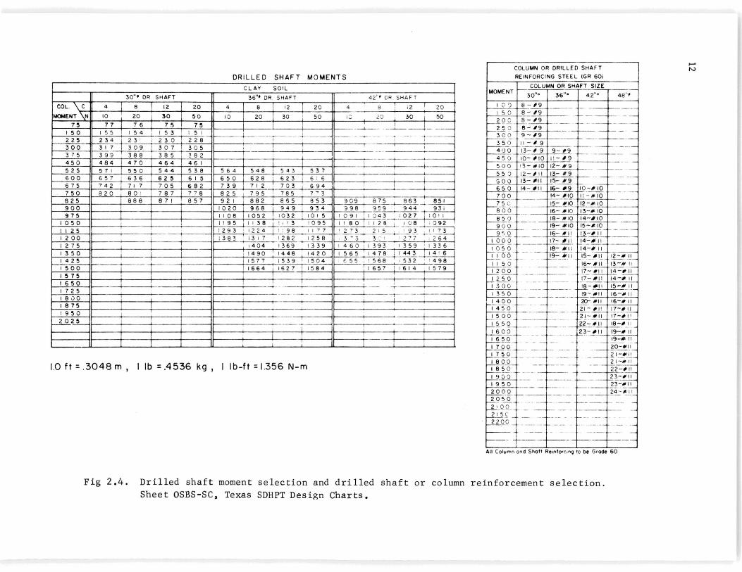
Step 3: from sheet OSBS-SC (Fig 2.4), select the shaft moment and shaft
and column reinforcing. Using a column moment of 600 ft-kips, N = 30 and
the table for Clay Soils, a shaft moment of 625 ft-kips (847 kN-m) is given
for a 30-inch-diameter shaft and 623 ft-kips (845 kN-m) for a 36-inch-diameter
shaft. Both shaft moments are rounded up to 650 ft-kips (881 kN-m) and the
reinforcement is chosen from the table, Column or Drilled Shaft Reinforcing
Steel (GR 60). From this table the values chosen are 14 No. 11 bars for a
30-inch shaft and 16 No. 9 bars for a 36-inch shaft. For the 30-inch column,
13 No. 11 bars are chosen.
Table 2.1 shows a summary of the design. As shown in the table, a cost
estimate was made for two combinations of shaft and column sizes.

TABLE 2 • 1. SUMMARY OF SHAFT DESIGN USING SDHPT DESIGN CHARTS
Shaft Diameter/Column Diameter
Column Moment, ft-kips
Column Reinforcement
Shaft Moment, ft-kips
Shaft Reinforcement
Shaft Length, feet 1
Approximate Dollar Cost of Concrete
Steel, lb
Approximate Dollar Cost of Steel1
Total Approximate Cost2
36"/30"
594
13 :f! 11' s
623
16 :f! 9' s
17
$954
925
$370
$1324
30"/30"
594
13 :ffo 11 1 S
625
14 1ft 11' s
18
$700
1338
$535
$1235
1 Based on lettings in Dallas, August 1979, concrete = $212/c.y., steel $ 0.40 per lb (U.S. dollars)
2 Does not include column superstructure, truss, signs, etc.
1 ft 0.3048 m
1 ft-k 1.356 kN-m
1 k 0.4536 Mg
15

16
Differences in design length are small; however, because the area of a
36-inch shaft is about 45 percent greater than that of the 30-inch shaft,
there is a significant increase in total concrete yardage for the 36-inch
shaft. There is more steel required for the 30-inch shaft but this increased
cost is offset by the differences in cost of the concrete. For the unit
prices that were used, the 30-inch shaft is the most economical choice.
Variances in unit prices between steel and concrete could obviously change
this conclusion and each case must be investigated to find the most economical
design under prevailing market prices. This completes the design using the
SDHPT design charts.
ANALYSIS USING COM623
Formulation of Data Set for Computer Solution
The system as design by the SDHPT charts was analyzed with the aid of
COM623. The given values, as required for design with the SDHPT charts, left
other values to be assumed as necessary for analysis by the computer. These
additional parameters were selected on the basis of information given in the
literature. The given values, as previously stated, were height = 30 feet, 2 span = 140 feet, and cQ = 1730 lb/ft for a clay soil. In addition, a
value of horizontal load of 18.3 k (87.4 kN) was obtained from sheet OSBC-SC-Z4
(Fig 2.3). The truss weight was 13.8 k (61.2 kN). The column weight was com
puted as 22.1 k (98.3 kN) using 150 1b/ft3 (23.6 kN/m3 ) for the weight of
concrete. The total axial load was therefore 22. 1 k + 13.8 k = 35.9 k
(160.0 kN). The moment at the shaft head was computed by adding the product
of the wind load times the sign height to the value obtained from Fig 2.3.
34.8 ft-k + 18.3 k (30) feet = 583 ft-k (790 kN-m) .
The soil as presented in the design charts was both homogeneous and of
constant strength with depth. The soil was modelled as a stiff clay above the 3 3
water table, with an effective unit weight, y, of 115 lb/ft (18.1 kN/m) 2
and an undrained shear strength, cQ , of 1730 lb/ft . From the literature,
values of strain at 50 percent of failure, e50 , of 0.010 and an initial
of 5.0 X 10⁵ lb/ft3 (7.86 X 10⁷
kN/m3
) k s modulus of subgrade reaction,
were assumed. Since the SDHPT charts were presented with
constant soil properties with depth, the parameters used in
17
the computer analysis were also made constant with depth. The diameter of the
shaft was selected as 30 inches to agree with the result from the SDHPT
procedure. The gross moment of inertia for a 30-inch circular section is about 4 4 6 . 2 7 2 39,800 in. (0.01657 m ). A value of 3.0 X 10 .lb/1.n. (0.0683 x 10 kN/m)
was used for the modulus of elasticity of concrete ( E ) . c
Variation of Parameters Used in Computer Solution
The value of several parameters were varied in turn to establish the
general behavior of the foundation. The effect of change in length was ob
tained by analyzing the shaft using lengths such that the full range of
behavior occurred, from the "fence post" (rigid body) action of short piles to
the "infinite pile" (flexible member) action of long piles. In addition, the
relative position of the water table was varied. This was accomplished by
using the total unit weight of the soil, yT , for the case where the water
table is well below the shaft tip and the buoyant u~it weight of the soil
( yT = yT - Yw ) for the case where the leve 1 of the water table is at the
shaft head. Effects of variation in the flexural rigidity of the shaft were
also investigated. Analyses were made using both the gross moment of inertia
previously mentioned, Igr , and an uncracked, transformed moment of inertia,
I , in which the steel areas were transformed but it was assumed that the tr
section remained uncracked. Shaft loadings were also varied from values of
0.7 Pt to 2.0 Pt and were applied in both a cyclic and a static manner.
This manner of loading is explained subsequently. Center for Transportation
Research Report 244-1, "Analysis of Single Piles Under Lateral Loading"
(Ref 5), makes use of the same variations plus variations of additional param
eters such as undrained shear strength and strain at 50 percent ( e50 ).
Although parametric studies in Report 244-1 were conducted on reports from the
literature, the basic pattern of behavior will be similar in all cases.
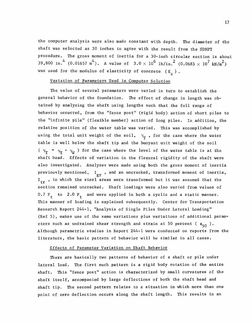
Effects of Parameter Variation on Shaft Behavior
There are basically two patterns of behavior of a shaft or pile under
lateral load. The first such pattern is a rigid body rotation of the entire
shaft. This "fence post" action is characterized by small curvatures of the
shaft itself, accompanied by large deflections of both the shaft head and
shaft tip. The second pattern relates to a situation in which more than one
point of zero deflection occurs along the shaft length. This results in an
18
increased curvature of the shaft. However, both the head and tip deflection
are reduced. The deflected shapes of the shaft, analyzed at lengths of 18 feet
and 26 feet, are shown in Fig 2.6. It is obvious that the shorter shaft has a
greatly increased groundline deflection, about 3-1/2 times larger than that of
the longer pile. In addition, an increase of shaft curvature is also apparent
for the long shaft, resulting in a small increase in bending moment. The
bending moment is 616 ft-k (835. kN-m) for the long shaft as compared to
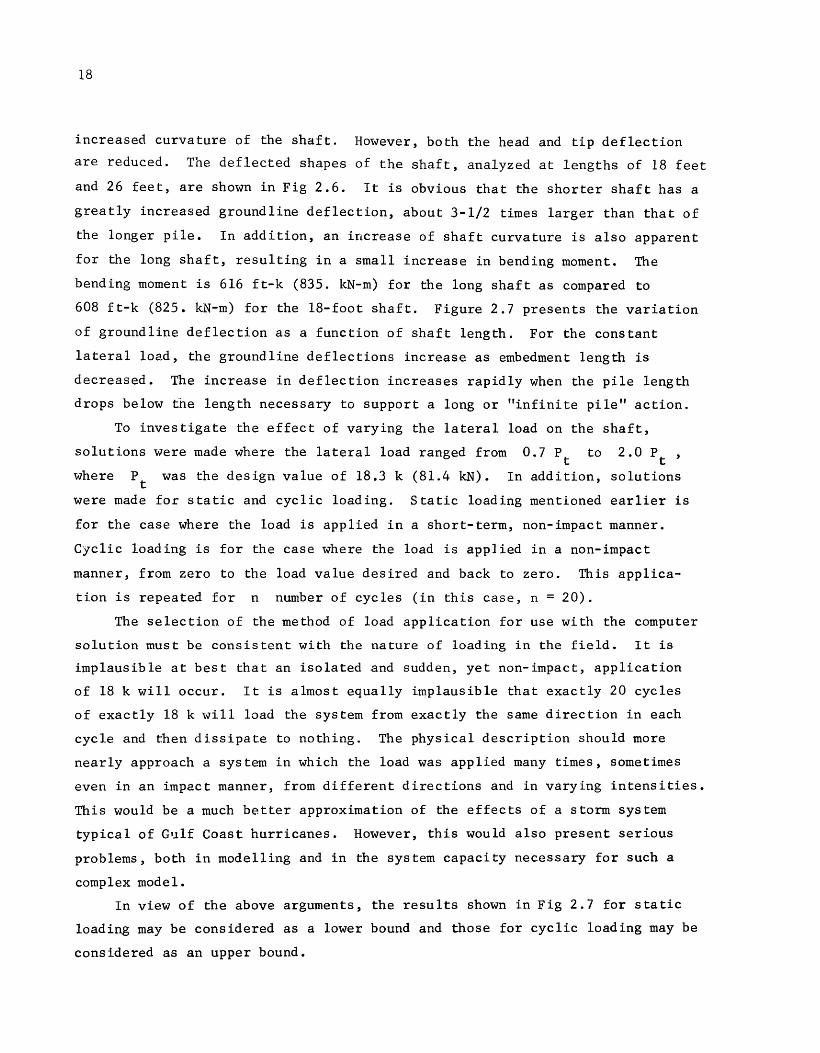
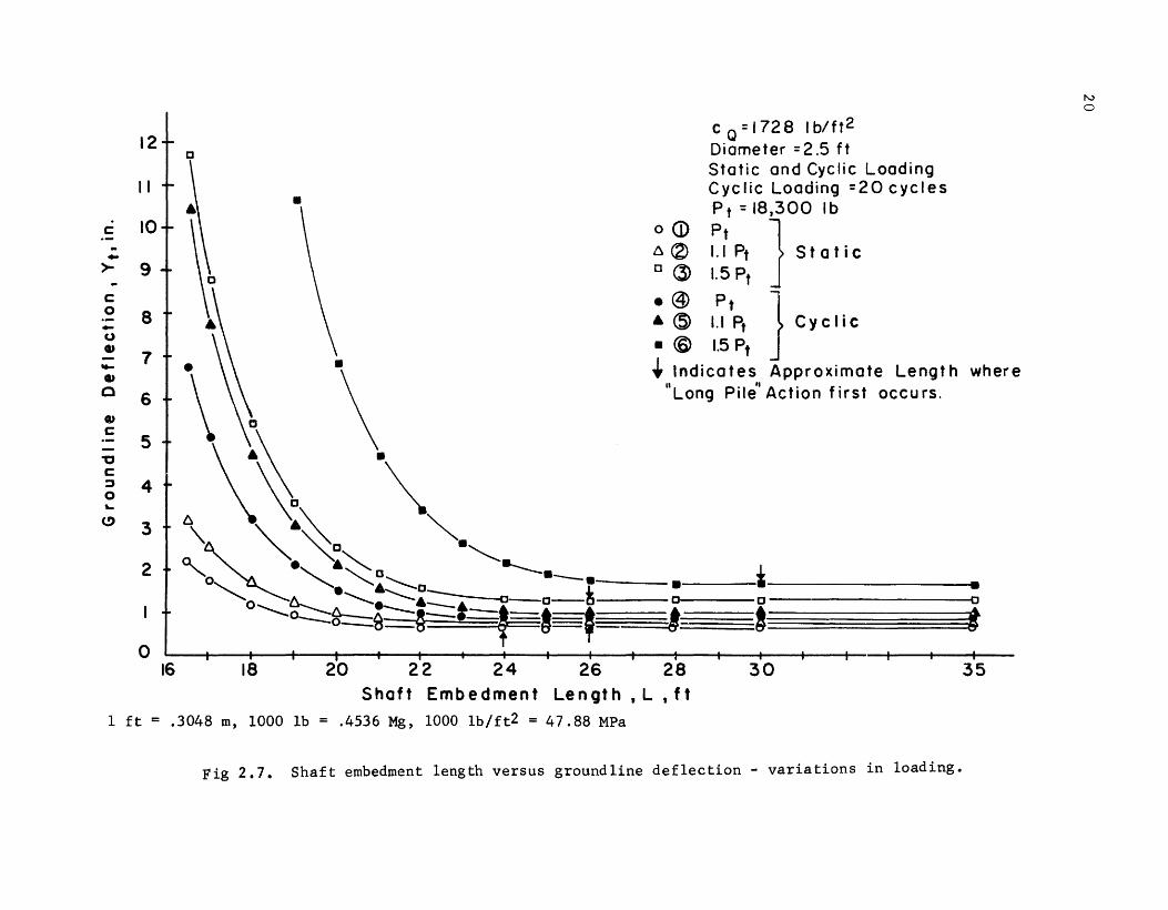
608 ft-k (825. kN-m) for the 18-foot shaft. Figure 2.7 presents the variation
of groundline deflection as a function of shaft length. For the constant
lateral load, the groundline deflections increase as embedment length is
decreased. The increase in deflection increases rapidly when the pile length
drops below the length necessary to support a long or "infinite pile" action.
To investigate the effect of varying the lateral load on the shaft,
solutions were made where the lateral load ranged from 0.7 Pt to 2.0 Pt ,
where Pt was the design value of 18.3 k (81.4 kN). In addition, solutions
were made for static and cyclic loading. Static loading mentioned earlier is
for the case where the load is applied in a short-term, non-impact manner.
Cyclic loading is for the case where the load is applied in a non-impact
manner, from zero to the load value desired and back to zero. This applica
tion is repeated for n number of cycles (in this case, n = 20).
The selection of the method of load application for use with the computer
solution must be consistent with the nature of loading in the field. It is
implausible at best that an isolated and sudden, yet non-impact, application
of 18 k will occur. It is almost equally implausible that exactly 20 cycles
of exactly 18 k will load the system from exactly the same direction in each
cycle and then dissipate to nothing. The physical description should more
nearly approach a system in which the load was applied many times, sometimes
even in an impact manner, from different directions and in varying intensities.
This would be a much better approximation of the effects of a storm system
typical of Gulf Coast hurricanes. However, this would also present serious
problems, both in modelling and in the system capacity necessary for such a
complex model.
In view of the above arguments, the results shown in Fig 2.7 for static
loading may be considered as a lower bound and those for cyclic loading may be
considered as an upper bound.

11 1 nf i ni te" or 11Lon g
Pi le• action (Fiexi ble)
'-.. Fence Post" or 11 5hort Pile' action (Rigid)
0 L= 18ft (5.5 m.)
• L = 26 f t (23.8m.)
Diameter = 2.5 ft (.76m)
Fig 2.6. Deflected shapes - rigid and flexible behavior.
1-' ~
c:
-->-c: 0 -u 41)
.... 41)
0
Cl)
c:
"0 c: ::J 0 ~
C.!)
12
II
10
9
8
7
6
5
4
3
2
0 16
0
•
•
c Q = I 7 2 8 I b/ f t 2 Diameter = 2.5 ft Static and Cyclic Loading Cyclic Loading =20 cycles Pt=l8,300 lb
o <D Pt ] 6 (2) I. I Pt S t a t i c c (3) 1.5 Pt
•@ Pt } • <5> 1.1 Pt Cyclic • ® 1.5 Pt
+ Indicates Approximate Length where "Long Pile" Action first occurs.
a..__'-.. ""'-·~ ll~:--....._o-----.,_a-~ ·o"-._~~.::::::i::::t-!==8 ,,~~======== .........._o_::::o-8- f
18 20 22 24 26 28 30 35 Shaft Embedment Length, L, ft
1ft= .3048 m, 1000 lb = .4536 Mg, 1000 lb/ft2 = 47.88 MPa
Fig 2.7. Shaft embedment length versus groundline deflection- variations in loading.
N 0
21
The cyclic-loading method is thought to be applicable to the design of
overhead-sign structures because wind velocity is seldom constant. The
gusting of the wind will cause repeated loadings to occur on the foundations.
It is known that a degradation of the soil resistance occurs with cyclic
loadings and the loss in soil resistance can be quite severe (Ref 4). The
increased deflections caused by a lessening of soil support can be accompanied
by an overstress of structural elements. Therefore, it is important to know
not only the behavior of the system subjected to a given load but also the
behavior of the system under cyclic loading.
The curves presented in Fig 2.7 represent changes in both load intensity
and method of load application. Curves 1 through 3 indicate the behavior to
be expected due to an increase in load, as do curves 4 through 6. In general,
both sets of curves exhibit the same characteristics. It is of interest to
note that the ratio of cyclic to static deflection increases as the shaft
length approaches that for rigid-body behavior. For example, at the design
load with a shaft length of 26 feet (7.9 m) the ratio is 1.31, while for a
length of 18 feet (5.5 m) the ratio is 2.7.
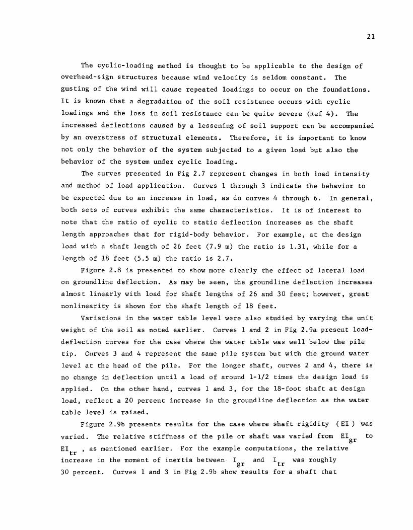
Figure 2.8 is presented to show more clearly the effect of lateral load
on groundline deflection. As may be seen, the groundline deflection increases
almost linearly with load for shaft lengths of 26 and 30 feet; however, great
nonlinearity is shown for the shaft length of 18 feet.
Variations in the water table level were also studied by varying the unit
weight of the soil as noted earlier. Curves 1 and 2 in Fig 2.9a present load
deflection curves for the case where the water table was well below the pile
tip. Curves 3 and 4 represent the same pile system but with the ground water
level at the head of the pile. For the longer shaft, curves 2 and 4, there is
no change in deflection until a load of around 1-1/2 times the design load is
applied. On the other hand, curves 1 and 3, for the 18-foot shaft at design
load, reflect a 20 percent increase in the groundline deflection as the water
table level is raised.
Figure 2.9b presents results for the case where shaft rigidity (EI) was
varied. The relative stiffness of the pile or shaft was varied from EI to gr EI , as mentioned earlier. For the example computations, the relative
tr increase in the moment of inertia betweP.n I and It was roughly gr r 30 percent. Curves 1 and 3 in Fig 2.9b show results for a shaft that
L=3o'1• / Static:!.A j
1.9 t L=26 6 • A Static / j /
1.8
1.7 "0 0 0 ..J 1.6
c: 0\ 1.5 (/)
Q)
0
0 -"0 0 0 ..J
-0 ~
Q) -0 ~
..... 0
0 -0
1.4
1.3
1.2
1.1
1.0
.9
6•• ~0
ll/ / Ill / rr / 0
ll o/0
------.
If / ------fj /0 ~· /i 1° /. Iii /. til /.
t:::M;j •
c 0 =1728 lb/ft2
Diameter = 2.5 ft. Static and Cyclic Loading Cyclic Loading = 20 cycles Pt = 18,300 lb
_b_ o CD 1a' 6~ 26
1
0 (3l 30 1
• @ 18 1
• <5 261
• ® 301
}static
}cyclic
JJ/1 07'11 I I I I I I I I I I I I I I
. 2 3 4 5 6 7 8 9 10 II 12 13 14 15
cr .8
Groundline Deflection, Yt, in.
1ft= .3048 m, 1000 lb = .4536 Mg, 1000 lb/ft2 = 47.88 MPa
Fig 2.8. Groundline deflection versus lateral load - load and length variations.
1'-.::. N

2.0
1.9
1.8
1.7
1.6
1.5 -CL
... 1.4 -c 0 0 _. 1.3
~ 1.2 Q) -0 _. 1.1
1.0
. 9
llA
II II
jj jj
)j 1
c Q = 172 8 I b If t 2
Diameter = 2.5 ft
Cyclic Loading =20 cycles
o(j)/'T ,L =18ft
ll~l T ,L =26ft
• ®0.45 J!r, L =18ft [email protected] fT, L =26ft
1 I l 0/.7°
1 /;:./ I 0 •
6 j/ .71 111 I I
.8
2 3 4 5 6 7 8 9 0
All
II /! jj jj II
A6
II A6
II All
li II
6A
II 1 II I ~ 0
II I 2 3 4
CQ = 1728 I b/ ft 2
Diameter= 2. 5 ft
Cyclic Loading =20cycles
0 CD Igr , L = 18 f t
6 ~ I gr • L = 26 f t
•@Itr ,L =18ft A@ I tr , L =26ft
~
5 6 7 8 9 (a) Groundline Deflection, Yt ,in. (b) Groundline Deflection, Yt , in.
1 ft = .3048 m, 1000 1b = .4536 Mg, 1000 lb/ft2 = 47.88 MPa, 100 lb/ft3 = 1.602 Mg/m3
Fig 2.9. Groundline deflection versus lateral load - variations in shaft moment of inertia and unit weight of soilo
N (..,.;)

24
was 18 feet long, with the moment of inertia being varied, as shown. The
figure indicates that the stiffness of the shaft for a short shaft has little
effect on overall deflections. Curves 2 and 4 show results where the moment
of inertia of a 26-foot shaft was varied. There is a noticeable change in
deflections; there is a relative increase of 25 percent at design load.
However, the actual increase in deflection is small, from approximately
0.67 inch (1.7 em) to 0.85 inch (2.16 c.m), or about 0.2 inch (0.51 em).
The variations in the parameters mentioned lead to several conclusions.
These may be summarized as follows.
(1) Deflections are sensitive to both shaft length and nature of load iP.g.
(2) Stiffness of the shaft has a relatively small effect on the deflection pattern.
(3) Changes in soil unit weights will not have a great effect on shaft deflection although relatively short shafts will be affected more than longer shafts.
COMPARISON OF COMPUTER SOLUTION TO DESIGN-AID SOLUTION
Use of the charts resulted in selecting a design shaft length of 18 feet
(5.5 m) for a 2.5-foot (76.2-cm)-diameter shaft. Curve 1 in Fig 2.7 shows
that the 18-foot shaft will behave as a rigid body under a static loading.
The deflection of the shaft head is approximately 1.2 inches (3.1 em), well
within the 3-inch limit established for the charts. The slope at the shaft
head is 0.74°, well within the limits set for slope. The computer analysis
was used to calculate the soil reaction at various points along the pile
according to the formula
p E y s
At the shaft base, p = 1218 lb/ in. , whereas is 2807 lb/in. and
(2 .1)
0. 7p u
is 1965 lb/in. Factors of safety were then computed based on the following:

and
where
Pmax p
and
for deflection
for slope
for soil reaction
s t
are the deflection and slope at the shaft head,
25.
(2 .2)
(2.3)
(2 .4)
p is the
greatest value of soil reaction occurring along the shaft, and Pmax , Ymax ,
and s are the maximum allowable values established for soil reaction, max
deflection, and slope. The values of factor of safety thus computed are
deflection 3 2.5 1.2
slope 2 2.7 .74
soil reaction 1965 1.6 1218
These values indicate that the chart gave a shaft length for the example
problem such that the limits established for behavior of the drilled shaft
were not exceeded.

!!!!!!!!!!!!!!!!!!!"#$%!&'()!*)&+',)%!'-!$-.)-.$/-'++0!1+'-2!&'()!$-!.#)!/*$($-'+3!
44!5"6!7$1*'*0!8$($.$9'.$/-!")':!

CHAPTER 3. ANALYSIS AND DESIGN OF DOUBLE-SHAFT SYSTEMS
APPLICATION OF LOAD
The basic configuration of the double-shaft system was mentioned in
Chapter 1. In brief review, the loading of the sign structure produces both
lateral loads and moments, which are transmitted by vertical trusses to the
foundations. The lateral forces are transmitted ~o the shaft heads as shears
while the moment is transmitted as a couple by the truss action. The couple
causes a tensile force on one shaft and a compressive force on the other. The
design of the shaft or pile must, therefore, account for both axial and
lateral forces. Appropriate care must be taken in the design process to
insure the adequacy of the shaft for resisting the axial forces in light of
the fact that the bending and deflection of the shaft under the lateral load
have an influence on its axial behavior. The first step in the process is to
formulate a design procedure for the axial loadings. The second step is to
check the influence of the shear and moment on the axial solution. There are
two recommended design procedures for axial loadings; one for compressive
forces and the other for tensile forces. The case for tensile forces is
treated first.
ANALYSIS OF A SHAFT SUBJECTED TO TENSILE LOADING
Alexis Sacre proposed a method of design based on experiments conducted
on several test shafts (Ref 16). Equations are advanced for determining the
capacity of a shaft when loaded by an uplifting (tensile) force. Cohesive
soils, clays and clay-shales, and cohesionless soils are considered.
27

28
COHESIVE SOILS
Several factors are involved in the computation of the shaft capacity.
The most obvious factor is the soil type. For clays, the following equation
for the shaft capacity is given:
where
p u f ( L - 5 ) n d + ~v '
P ultimate uplift capacity of the shaft, u
L length of the shaft,
d diameter of the shaft,
W effective weight of the shaft (accounting for buoyancy),
f side friction,
0' CQ '
= correlation factor (see Table 3.1), and
cQ undrained shear strength of clay.
(3 .1)
P is the ultimate capacity of the shaft to resist pullout. The first term u
in Equation 3.1 represents the capacity of the shaft developed by the inter-
action of the soil and shaft. In this first term the quantity f is the
"side friction" (also termed "skin friction"), with f as a function of the
soil shear strength. Various factors such as construction technique, soil
properties, arrd concrete condition \vill affect the capacity of the soil to
develop a given loading. The factor 0' attempts to account for this varia
bility (Ref 11). Figure 3.1 shows values of 0' that were computed from a
number of load tests. There appears to be a large scatter in the results;
however, some of the tests from London were not performed using modern con
struction techniques. The tests performed by The University of Texas, not
using the residual cohesion, are thought to be most representative.
In addition to the reduction of the soil capacity by the 0'-factor, the
top 5 feet of the shaft should not be counted on to contribute to the shaft

I. 2 5 I
0 Tests in London clay
c Tests performed by U T
1.00 t- 121 Values of a. obtained using a residual cohesion
c c
c:J I c .. 0.75
'-0 4-
0 c c 00 c ~ 1.1.. 0
~0 c
g 0.50 ~
0 4-
0
~ 0 c
:::J
00 fl>~ 0
-o 0 Q)
a: 0.2 5 0 21 21 21
0 0 0.5 1.0 1.5 2.0 2.5 3.0 3.5
Undrained Shear Strength of Cia y , tons/ ft.2
1000 lb/ft2 47.88 MPa
Fig 3.1. Correlation factor, a, for design of shafts in tension. !IV \.0
30
capacity. The first term therefore is seen as the capacity of the soil to
resist the load in the shaft. I
The second term, W , is simply the net weight
of the shaft itself, taking into account the buoyant effect of the water.
The value of a to be used in Eq 3.1 may be selected as 0.6 for good
construction methods, for example, with the dry method of construction if the
excavation is not allowed to remain open for many hours. If there is an
inward deformation of the soil due to creep there can be a reduction in shear
strength. In such cases and in other instances of questionable construction
procedures, the value of a should be reduced (Ref 12).
The limit on side shear for clays is nominally 2 tons/ft2 but values of
load transfer much larger have been measured in experiments in shale, as dis
cussed below. The limit in side shear is established as the maximum value
that has been measured in experiments with instrumented drilled shafts.
For drilled shafts in clay-shales that are subjected to tensile loading,
the uplift capacity may be computed by use of Eq 3.1. The same values for a
can be used for the clay-shales as for the clays; however, load transfer
values as high as 7 tons/ft2
have been measured in a test of an instrumented
drilled shaft (Ref 1). Load transfer values of such a magnitude would need to
be used with caution, of course, because of the small number of load tests
that have been performed on instrumented drilled shafts in clay-shale.
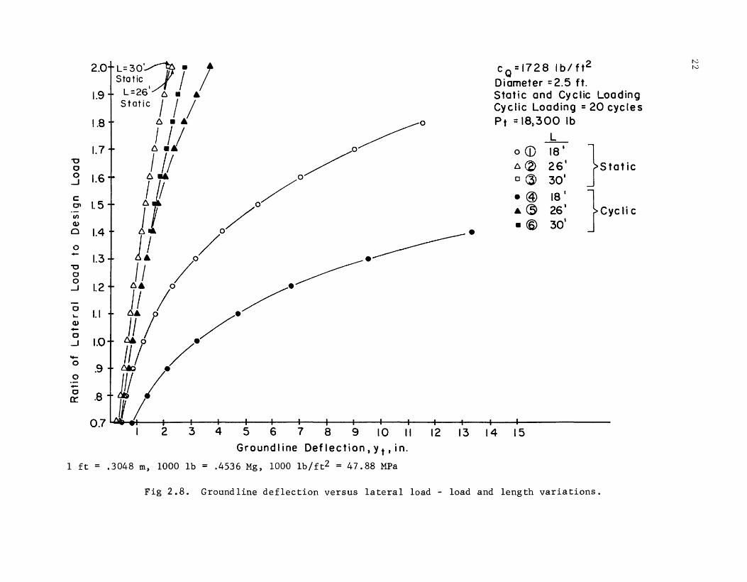
The assumption implicit in Eq 3.1 is that the shaft is straight-sided.
If an underream is added, the capacity of the shaft is changed and the
capacity of the underream is added to that of the shaft previously computed
using Eq 3.1 except that the length of the shaft must be reduced. Underream
capacities can be computed by the following formula:
where
(c F +- lF )(D2 - d2 ) Q c y q n 4
Qu uplift capacity of the underream,
cQ undrained shear strength of clay or shale,
F and F are breakout factors for clay and sand, c q
respectively (see Figs 3.2 and 3.3),
~ 1- 1.5D - S (see Fig 3.4),
(3.2)

0
2
3 C)
....... _J 4
.J::, ... 5 a.
Q)
0
Q) 6 > ... 0 7 Q)
a:: 8
9
10
0 2
Fig 3.2.
Breakout Factor, Fe
3 4 5 6 7 8
Breakout factor, F , for clay soils. c
31
9

0'
80
60
40
LL20 .. '-0 -0 0 LLIO
- 8 ::l 0 ~ 6 0 (I)
'-CD 4
2
l 0
---------~-------
,..,.,~
~.,.,
-~ -~ n. ---/__...-"" ... ~v ..-..-~·/ ~ s ... __ .....
h.'/" 0~~:_ ...... ./ ..... -~'?' __.... .............
./ .~ ..... ~ /.
h~/·· '/·
/ .• /· '/.
/.· --------- - - ---- ,_- ---- ------/
/0 ~/,
~-/ Balla
Sutherland
Baker a Kondner
---- Esquivel
2 3 4 5 6 Relative Depth, LID
Fig 3.3. Breakout factor, F , for sand soils. q
7
--- -----
Esquivel
Sutherland
Theory ( Vesic)
8 9 10
w N
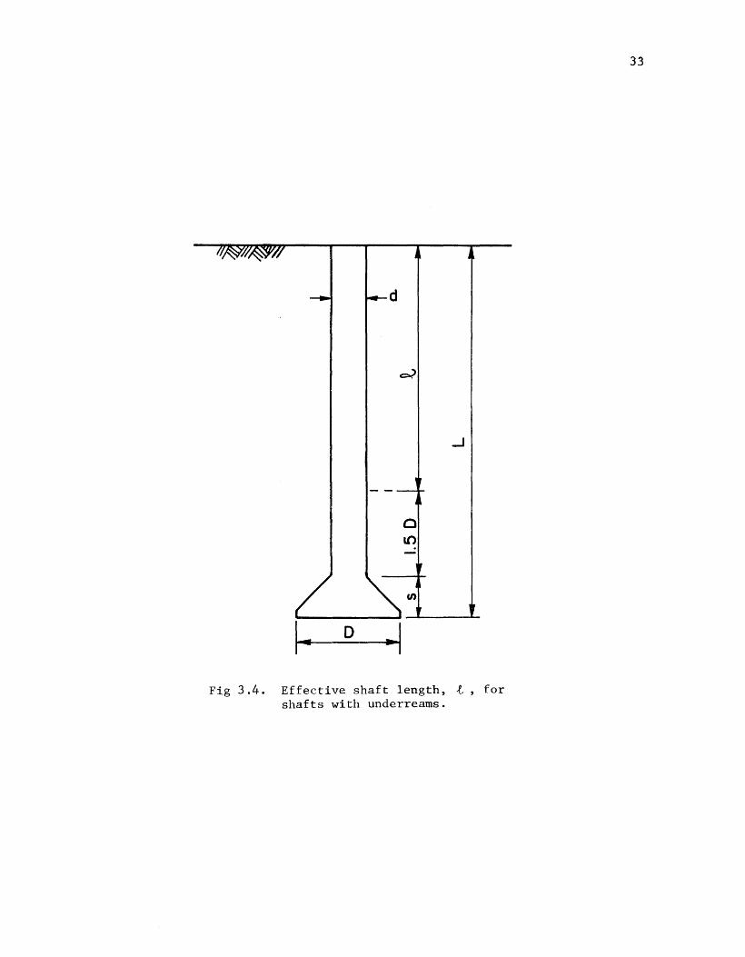
d
I~ D
Fig 3.4. Effective shaft length, t, for shafts with underreams.
33
34
L depth to base of bell,
S height of bell,
D diameter of bell, and
d diameter of shaft.
While Eq 3.2 deals with the case where the underream is cut into sand, it
is rare when such a construction procedure is possible. An underream cut into
sand could very well collapse even though drilling fluid is employed to main
tain the shape of the excavation.
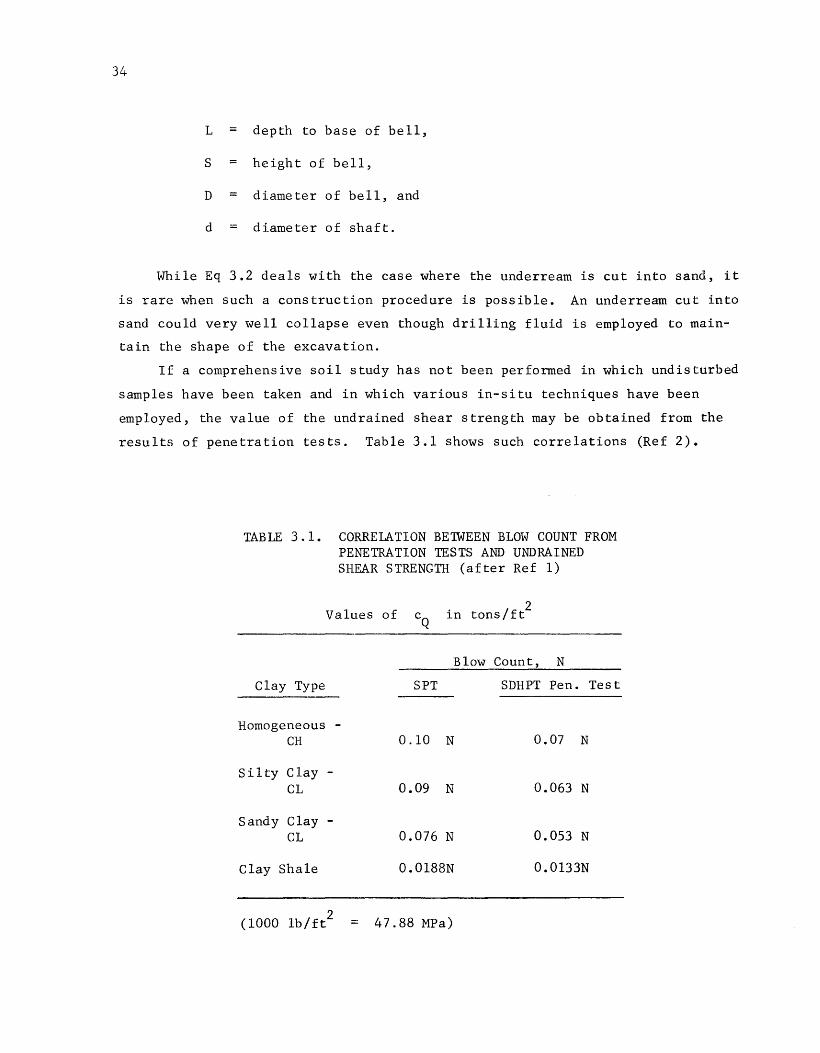
If a comprehensive soil study has not been performed in which undisturbed
samples have been taken and in which various in-situ techniques have been
employed, the value of the undrained shear strength may be obtained from the
results of penetration tests. Table 3.1 shows such correlations (Ref 2).
TABLE 3.1. CORRELATION BETWEEN BLOW COUNT FROM PENETRATION TESTS AND UNDRAINED SHEAR STRENGTH (after Ref 1)
Values of
Clay Type
Homogeneous -CH
Silty Clay -CL
Sandy Clay -CL
Clay Shale
in tons/ft2
Blow Count, N
SPT SDHPT Pen. Test
0.10 N 0.07 N
0.09 N 0.063 N
0.076 N 0.053 N
0.0188N 0.0133N
(1000 lb/ft2
47.88 MPa)

.35
COHESIONLESS SOILS
The tensile capacity of a straight-sided shaft in cohesionless soils is
given by Eq 3.3:
where
p u
f u
2 + (L - d ) f J n d + w 1
u u
P uplift capacity of shaft, u
f u
d u
= ultimate side resistance (see Fig 3.5),
depth at which
f u
y K tan '0
f occurs, u
y effective unit weight of sand,
K = lateral earth pressure coefficient,
0 = angle of internal friction of sand,
L shaft length,
d shaft diameter, and
I
W effective weight of shaft.
Side resistance increases from 0 at the groundline to some limiting
(3. 3)
value, f , at depth, d Figure 3.5 presents f values as a function of u u u
the Standard Penetration Test (SPT) blow count (Ref 13). For SDHPT purposes,
correlations between the SDHPT pen test and SPT have been made (Ref 18). As
in the equation for clay soils, the first term is the capacity of the soil to
resist the loading and the second term is the effective weight of the shaft.
As an example of the use of Eq 3.3, assume that a drilled shaft that is
4 feet in diameter has been installed in a sand with a 0 of 40 degrees and a
submerged unit weight of 60 lb/ft3 . A value of 0.7 is selected for K.
Using Fig 3.5, the ultimate side resistance is 1.38 tons/ft2
. The depth d u
at which this ultimate side resistance will develop is computed to be 78.3 ft.

36
C\1 .... 'to-
' en c 0 .... -cv
3.0
~ 2.0 c .... en en cv a:: cv
"C
en cv .... c E
:;:: 1.0 ::>
Approximate Angle of Internal Friction , <t>
30 35 40 45 dense
010.2
018.0
10.2 0 018.0
018.3
046.7
046.7
very dense
010.2
029.4
Note:
150 18.0 0--+
130 18.0 o..:..;.;
Number beside point is the depth- to- width ratio
0 ~------------~--------~----------~----------~----------~ 0 20 40 60 80 100
Number of Blows in the Standard Penetration Test
Fig 3.5. Ultimate side resistance, f , for design of shafts in tension. u

37
Therefore, the side resistance at 40 feet would be 0.70 tons/ft2 . Thus, the
first term in Eq 3.2 yields a value of P of 176 tons. Had d been corn-u u
puted as less than 40 feet, Eq 3.3 would have been employed without change.
ANALYSIS OF A SHAFT SUBJECTED TO A COMPRESSIVE LOADING
A drilled shaft under compressive load usually distributes its load to
the supporting soil both in skin friction and end bearing. The relative
magnitude of the load carried in skin friction and end bearing depends princi
pally on the nature of the soil deposit but the shaft geometry will also play
an important role. The settlement of a drilled shaft under a given load will
also depend on the soil profile and on the geometry of the shaft. The follow
ing paragraphs present a review of methods of analysis of drilled shafts in
compression.
A basic formula for the computation of the capacity of a drilled shaft in
compression is given by Quiros and Reese (Ref 10):
(3.4)
where
Qs capacity of shaft in skin friction, and
Qb capacity of shaft in end bearing.
The categories of construction techniques are discussed in some detail else
where (Refs 10 and 11). As with the section on tensile capacity, the capacity
in compression is discussed first for cohesive soils and then for cohesionless
soils.
COHESIVE SOILS
For deposits that are predominantly clay, the values of Qs and Qb are
obtained from Eqs 3.5 and 3.6:

38
= (3. 5)
and
(3. 6)
where
CY correlation factor (Table 3 .. 2),
CQ average undrained shear strength,
Nc = bearing capacity factor (Table 3.2),
A area of shaft surface, and s
AB area of shaft base.
In addition to giving values of CY and NC , Table 3.2 shows the
portions of a drilled shaft in compression that are assumed to be noncontribu-
ting (Ref 6).
It should be noted that the construction categories have a significant
influence on the design parameters. The importance of the construction method
was noted in the discussion of the design of drilled shafts to sustain tensile
loadings. The construction categories are recognized in a more formal way in
Table 3.2, as follows:
Category A:
Subcategory A.l: Shafts installed dry or by the slurry dis
placement method.
Subcategory A.2: Shafts installed with drilling mud along some
portion of the hole such that entrapment of drilling mud between the
sides of the shaft and the natural soil is possible.
Category B: Underreamed drilled shafts in either homogeneous or layered
clay with no soil of exceptional stiffness relative to the soil around the
stem, below the base.
Subcategory B.l: Shafts installed dry or by the slurry dis
placement method.

TABLE 3.2. DESIGN PARAMETERS FOR DRILLED SHAFTS IN ClAY
Parameter
Side resistance* in clay 0'
avg
Limit on side shear ( tsf)
Tip resistance')''""'"' in clay N
c
(Primary Design Procedure)
Design Category
A .1 A.2 B.l B.2 c
0.6 0.3 0.15 c 0
2.0 0.5 0
9 9 9 9 9
39
D
0
0
9
aMay be increased to category A.l value for segments of shaft drilled dry.
bLimiting side shear 2.0 tsf for segments of shaft drilled dry.
cMay be increased to category B.l value for segments of shafc drilled dry.
dLimiting side shear 0.5 tsf for segments of shaft drilled dry.
*Equation for computing side resistance:
**Equation for computing base resistance:
+ Top 5 ft. Noncontributing
t
• Bottom One Diameter Noncontributing
t
CY s A avg u s
+ One Stem Diameter Above the Bell Noncont ri buti ng
J Periphery of Bell Noncontributing
t

40
Subcateg0ry B.2: Shafts installed with drilling mud along some
portion of the hole such that entrapment of drilling mud between the
sides of the shaft and the natural soil is possible.
Category C: Straight-sided shafts with base resting on soil significant
ly stiffer than the soil around the stem. The stiffer soil will not allow the
shaft side resistance to be developed.
Category D: Underreamed shafts with base resting on soil significantly
stiffer than the soil around the stem. The stiffer soil will not allow the
shaft side resistance to be developed.
Limiting values on side shear are also given in Table 3.2. If a detailed
analysis of the soil deposit is not available, the capacity may be computed
using the results of a Standard Penetration Test or an SDHPT Pen Test. The
contribution due to skin friction, Qs , is computed as in Eq 3.5, with values
of cQ being given in Table 3.1 (Ref 2) and Q in Table 3.2. However, for
the base capacity, Eq 3.8 must be used:
(3.8)
where
N blow count SPT or SDHPT Pen Test,
p1
correlation factor obtained from Table 3.3, and
AB area of the shaft base.
For the design of drilled shafts under compressive loads in clay-shales,
the procedures set forth for clay may be used except that the limiting siu2
resistance can be increased to as high as 7 tons per square foot and that the
bearing capacity factor N c should be decreased to 8.

TABLE 3.3. DESIGN PARAMETERS FOR BASE RESISTANCE FOR DRILLED SHAFTS IN CLAY
(After Quiros and Reese, 1977)
Design Category
Parameter A.1 A.2 B.1 B.2 c
p1 (SPT) 1.6 1.6 1.6 1.6 1.6
p1 (SDHPT) 2.8 2.8 2.8 2.8 2.8
Limit on bearing pressure (tsf) 35 35 35 35 35
Note: Equation for computing base resistance:
D
1.6
2.8
35
N p~
41

42
COHESIONLESS SOILS
For shafts used in sand deposits the same basic equation (3.4) is used.
The resistance to load offered by the shaft side surface is
where
where
=
c =
Q' avg
H ci
0 p tan ~ dz
circumference of the shaft,
H total depth of embedment of the shaft,
0 = effective angle of internal friction,
p
Q' avg
effective overburden pressure, and
correlation factor (Table 3.4).
For the base resistance
=
D
=
base diameter,
base capacity at 5 percent tip movement (Table 3.6), and
base movement factor (Table 3.5).
(3. 9)
(3. 10)
When the design procedure for drilled shafts in sand under compressive
loading is based directly on the results of penetration tests, the following
procedure may be used.
The equation for side resistance is
(3.11)

TABLE 3.4. DESIGN PARAMETERS FOR DRILLED SHAFTS IN CLAY-SHALE
(After Quiros and Reese, 1977)
Design Category
Parameter A B
Side resistance"~" in c1ay-shale 0' 0.75 0.50
avg
Tip resistance"~"* in clay-shale N 8 8 c
Category A: Shafts installed by the dry method
Category B: Shafts installed by che casing method
c
0.50
7
Category C: Shafts ins tal led by the slurry displacement method
-1.-Equa tion
"'"'*Equation
for computing side resistance: Qs
for computing base resistance: QB
TABLE 3.5. TIP MOVEMENT FACTOR, kf
"Base Diameter, D , ft
< 1.67
> 1.67
(1 ft = 0.3048 m)
(Y s A avg u s
Nc cQAB
1.0
0.6D
43
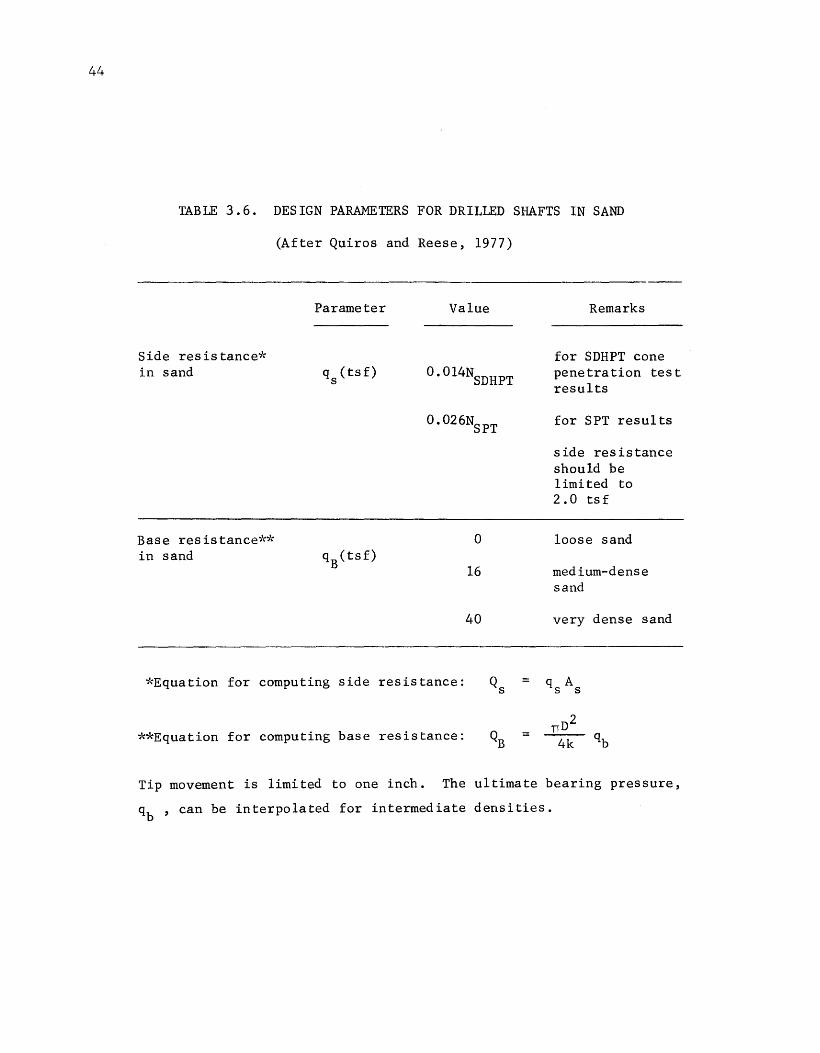
44
TABLE 3. 6. DESIGN PARAMETERS FOR DRILLED SHAFTS IN SAND
(After Quiros and Reese, 1977)
Parameter Value Remarks
Side resistance* for SDHPT cone in sand q (tsf) 0.014NSDHPT penetration test s
results
0.026NSPT for SPT results
side resistance should be limited to 2.0 tsf
Base resistance** 0 loose sand in sand qB(tsf)
16 medium-dense sand
40 very dense sand
*Equation for computing side resistance:
**Equation for computing base resistance:
Tip movement is limited to one inch. The ultimate bearing pressure,
qb , can be interpolated for intermediate densities.

where
qs load transferred along shaft sides (Table 3.6).
The equation for end bearing remains the same as before, with NSPT or
NSDHPT being used to ascertain whether or not the sand is loose, medium
dense, or very dense.
ADDITIONAL FACTORS AFFECTING SHAFT CAPACITY
45
In the case of clay soils, it has been pointed out that the top 5 feet of
shaft are to be ignored in computing the shaft capacity. This is due to
several factors. One major factor is the shrinkage of a desiccated soil layer,
which will result in poor or even no contact between the shaft surface and the
soil medium. It is also recognized that, on many occasions, the upper several
feet: of soil may be substantially weaker due to factors such as weathering,
fissuring due to cycles of expansion and contraction, the addition of organic
substance due to plant growth, and the decay of plant growth.
A factor that also affects clays and will affect some cohesionless soils
is the degradation of capacity near the surface due to lateral loadings and
deflections. Any lateral load will cause the shaft to deflect laterally. If
thi::: deflection is severe enough, a pronounced separation of the soil and
shaft will occur. For this reason, lateral loadings and deflections must be
accounted for within the axial design. This holds for both tensile capacities
and compressive loadings. In both cases the lateral deflections should be
analyzed and judgments made as to their effect on the skin friction capacities
of the shaft.
The factor of safety should be selected after a careful consideration of
all the elements affecting the design. In general, the best approach is to
compute the collapse load or the load that produces excess deflection and to
compute the factor of safety as the ratio of the computed ultimate load to the
working load.
46
AVAILABLE PROGRAMS FOR COMPUTER ASSISTED ANALYSIS OF SHAFTS IN COMPRESSION
The relative simplicity of the equations involved in computing the axial
capacities in compression allowed two computer programs to be developed as
aids for design. BSHAFT and SHAFTl allow computation of shaft capacities and
relative shaft efficiencies based upon load per unit volume. SHAFTl is used
when the soil properties are well known, i.e., it utilizes the basic soil
properties. BSHAFT makes use of input based upon the results of a dynamic
penetration test.
SHAFTl allows a sophisticated model of the soil-shaft system to be
developed. The soil system can be accurately modelled to reflect a layered
system if desired. In addition, the changing of all or some of the design
parameters is easily accomplished. BSHAFT does not allow the same modelling
capabilities as SHAFTl. However, the outputs of both programs are similar and
can be useful. The results can be used to generate graphs of shaft length
versus shaft capacity and can be further broken down into shaft capacity due
to skin friction and shaft capacity due to tip resistance (see Figs 3.6a and
3.6b). Both programs have the capability to make computations for a series of
shaft diameters. If several diameters are studied, a design for a "step
taper" type of foundation can be made. Further details for both programs can
be found in the Quiros and Reese report (Ref 12).
DESIGN OF CLOSELY SPACED SHAFTS
INTERACTION OF CLOSELY SPACED SHAFTS UNDER lATERAL LOADS
The design of any shaft that is subject to a combination of loadings must
account for the effect of each load. This has been pointed out in previous
paragraphs with reference to the interaction between lateral loads and deflec
tions and computation of axial capacities. For shaft groups, i.e., two or
more closely spaced shafts, the lateral deflection of any shaft in the group
is increased relative to a single-shaft deflection due to the influence of
adjacent shafts under load. The problem is not unique to any one application
and occurs not only for double-shaft foundations for overhead signing but also
for group piling for abutments, bents, retaining walls, and similar structures.
Several solutions to the situation have been advanced. Poulos has presented a
solution based upon elastic theory (Refs 9 and 10).

.... c (I)
.... E ..... "C 0 cv .C..o C/) E
w
N1 <N2 <N 3
N =SDHPT Blow Count
Pu
Ea) Typical shaft capacity vs. embedment length
Load Capacity
~Total Capacity , Pu
' Capacity due to end bearing
Capacity due to 11 Skin friction ..
(b) Typical breakdown of total shaft capacity vs. shaft length
Fig 3.6. Shaft capacity versus embedment length.
47

48
Proposed Methods of Analysis
Since PoulGs' solution is based upon the theories of elasticity,
solutions made for high levels of stress in the soil will be inaccurate. The
nonlinear response of soil to imposed stresses, like that of concrete, dic
tates that elastic theories be restricted to use with low stress levels where
the assumption of linearly elastic behavior is best approximated. In
addition, Poulos confines his solution to a constant value of soil modulus
( E ) and pile or shaft modulus ( E ) . While this may be acceptable for the s shaft, where material properties will most likely be constant or can be
approximated as such, the soil may and probably will have an E widely s
varying with depth or even horizontal location. In addition, the solution is
available only for fixed- and free-head piles or shafts and yields only the
deflections of the shaft or pile head. With these limitations in mind, the
Poulos solution can be utilized and, in fact, is partially utilized by Focht
and Koch to account for the deflections of a pile or shaft within a group
(Ref 3).
The method of solution proposed by Focht and Koch involves the combina
tion of Poulos' elastic solution with the nonlinear, subgrade-reaction
solutions proposed by Reese and Matlock (Ref 3). The former is an attempt to
provide a solution that recognizes that the stress levels imposed by the shear
load on individual shafts will cause plastic deformations and will be accom
panied by a lesser deformation caused by lower stress levels due to the inter
action of adjacent shafts. In a group, the total group load must be distrib
uted, though not equally, among the shafts. Each shaft will, therefore, be
acted upon by a horizontal load that will develop stresses within the soil
mass. Immediately adjacent to the shaft these stresses may become quite
large. However, as the load is distributed out into the soil mass, the
induced stress level diminishes. Boussinesq developed equations (based upon
the theory of elasticity) which attempted to quantify this phenomenon (Ref 7).
Therefore, the stresses at a pile will be increased, even if no load is
applied to that pile, if an adjacent pile is under load. Since these
stresses will normally be small, a solution for deflections due to these small
stresses and based upon the theory of elasticity will be satisfactory.
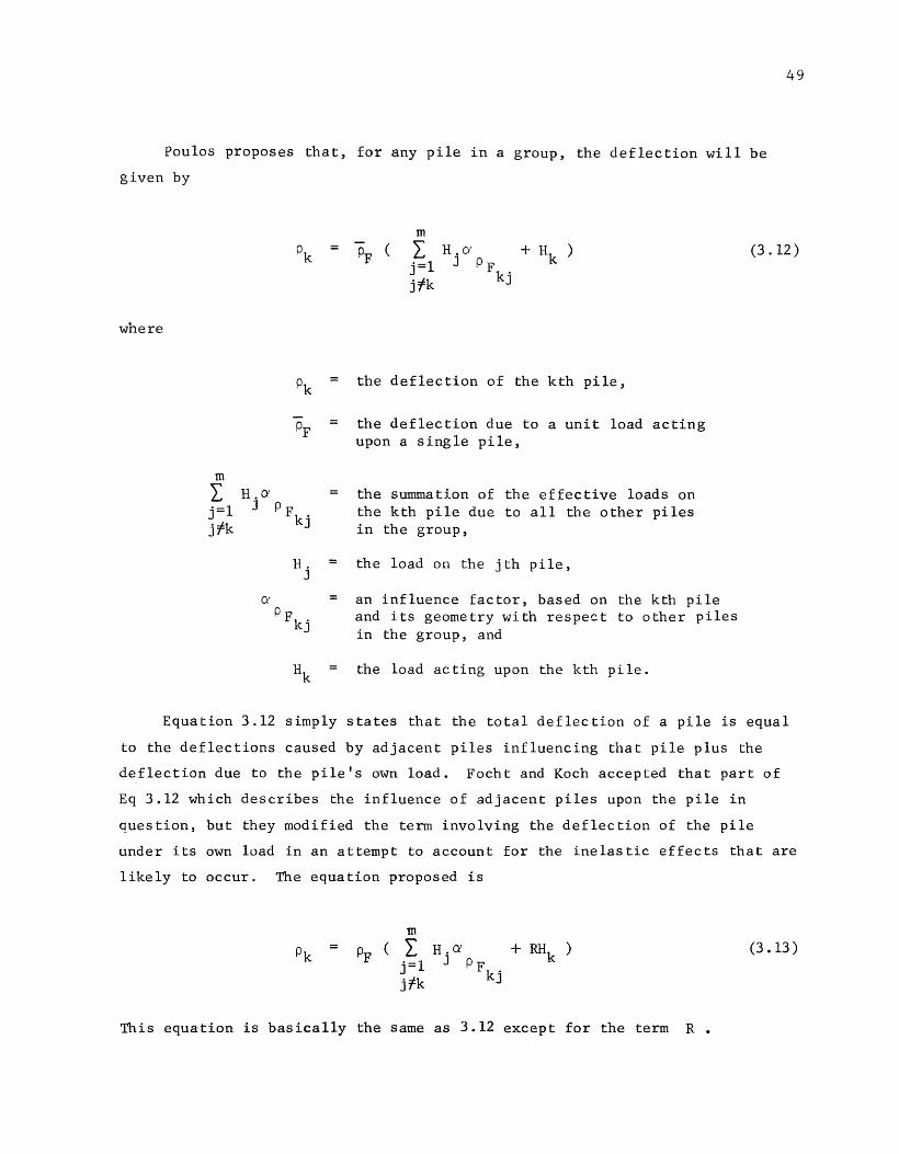
49
Poulos proposes that, for any pile in a group, the deflection will be
given by
where
m
I j=l j:fk
H.O:' J PF
kj
H. J
= m
I j=l j:fk
H.O' J PF
kj
the deflection of the kth pile,
the deflection due to a unit load acting upon a single pile,
the summation of the effective loads on the kth pile due to all the other piles in the group,
the load on the jth pile,
an influence factor, based on the kth pile and its geometry with respe~t to other piles in the group, and
the load acting upon the kth pile.
(3. 12)
Equation 3.12 simply states that the total deflection of a pile is equal
to the deflections caused by adjacent piles influencing that pile plus the
deflection due to the pile's own load. Focht and Koch accepted that part of
Eq 3.12 which describes the influence of adjacent piles upon the pile in
question, but they modified the term involving the deflection of the pile
under its own load in an attempt to account for the inelastic effects that are
likely to occur. The equation proposed is
= H.O:' J p F
kj
+ RHk )
This equation is basically the same as 3.12 except for the term R •
(3. 13)

50
where
Focht and Koch proposed that
R
R
p
a relative stiffness factor or ratio,
the deflection of an isolated pile calculated by p-y methods (i.e., the piles, "plastic" deflection), and
the deflection of an isolated pile calculated by the Poulos method (:i. .e., the piles "elastic" deflection).
Application of Analytical Method to Design
(3. 14)
The analysis and design of a multi-shaft or multi-pile group is based
upon Eq 3.13. Analyses of two-shaft groups will be the simplest to perform
although larger groupings ~ill only be more tedious, not more complex. In
general, the problem may be approached in the following manner:
(1) Determine the initial parameters for the pile or shaft and for the soil on the site, including loading on the group.
(2) Develop a set of p-y curves for a single pile or shaft.
(3) Compute ys , the groundline deflection, using COM623 and an
average load on the pile
(4)
where
H avg
=
m
total load on the pile or shaft group and
m number of piles in the group.
Select a value of Young's modulus for the soil, E , that s
represents a low stress level in the soil. An initial modulus from the laboratory stress-strain curves may be employed.
(3. 15)

(5) Using E s
from (4) and H from (3), compute the groundline avg deflection, pF , for a single pile using Poulos' method for a
single pile.
(6) With che results of (5) compute the deflection, unit Load as
pF , due to a
51
H avg
(3. 15)
(7) Compute R by dividing the value from (3), calculated in (5), pF .
y , by the value s
(8) Using the Focht-Koch equation (Eq 3.13), write an equation for each pile in the group. Influence coefficients, a , can
be obtained using graphs from Poulos. PFkj
(9) Write an equation of equilibrium for the shear load on the group, i.e.,
where
HT total load on group and
Hm load on roth pile.
(10) Solve the equations generated in steps (8) and (9), knowing that the deflection of each pile in the group must be equal. The group deflection and values of load for each pile will be obtained.
(3. 16)
(11) Use a set of y-multipliers (2, 3, 4 and so on) to modify the curves generated in step (2). Then compute groundline deflections using the load from step (10) and the modified p-y curves. This generates a relationship between groundline deflection and the y-multipliers.
(12) Using the relationship established in (11), find the value of the multiplier that will give the same deflection as that computed in step (10).
(13) Modify p-y curves by the factor obtained in step (12) and use the new set of curves to compute the bending moment produced in the pile or shaft that supports the largest load.
( 14) Check the adequacy of the pile or shaft des :i_gn, using the results of (13).
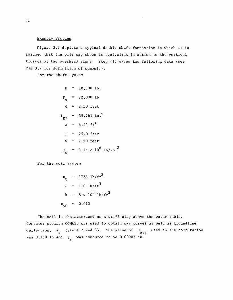
52
Example Problem
Figure 3.7 depicts a typical double shaft foundation in which it is
assumed that the pile cap shown is equivalent in action to the vertical
trusses of the overhead signs. Step (1) gives the following data (see
Fig 3. 7 for definition of symbols):
For the shaft system
H 18,300 lb.
p 72,000 lb X
d 2.50 feet
I 39,761 in. 4 gr
A 4.91 ft2
L 25.0 feet
s 7.50 feet
E 3.15 X 10 c
6 lb I in.
2
For the soil system
CQ 1728 lb/ft2
y 110 lb/ ft3
k 5 X 10⁵
lb/ft3
€50 0.010
The soil is characterized as a stiff clay above the water table.
Computer program COM623 was used to obtain p-y curves as well as groundline
deflection, ys (Steps 2 and 3) . The value of H used in the computation avg
was 9,150 lb and ys was computed to be 0.00987 in.
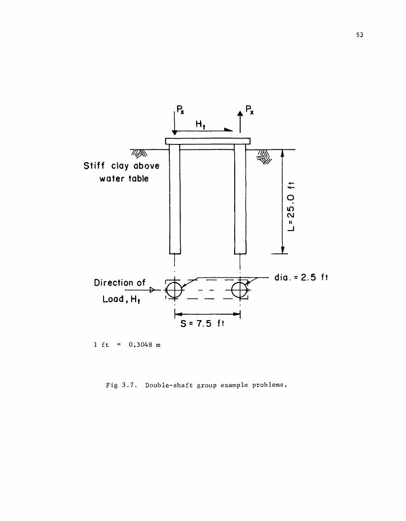
Stiff clay above water table
Di~:::o_,n_H_~_f ..Q~~ oc- _Qf ,.. ..., s = 7. 5 ft
1 ft 0.3048 m
-'+-
0 . lO N II _J
dia. = 2.5 ft
Fig 3.7. Double-shaft group example problems.
53

54
Step (4) requires the computation of
assumed that
E s
For this problem it is
Es 250cQ = 3000 lb/in.2
The elastic groundline deflection of a single pile or shaft may now be
computed by methods given by Poulos (Step 5).
where I is from Fig 3e8. PF
L/d
~ =
Use~
_12- = 2.5
EI
E 14
s
0.00515
5 X 10⁻³
10
(3.15 X 10⁶ lb/in.2
)(39,761 in.4)
(3000 lb/in. 2 )(300 in.)4
From Fig 3.8 generated by Poulos
I 3.5 PF
3.5 2 [
9150 lb
(3000 lb/in. )(300
0. 036 in.
The unit deflection is then computed (Step 6):
_2_ H avg
0. 036 inch 9150 lb

55
50
20 lfs= 0.5
Values of Lfd
I pF 10
5
2
Fig 3. 8. Influence factor I for fixed-head PF
piles (from Poulos, 1971).
56
= 3.93 X 10- 6 lb/in.
R is now computed (Step 7):
R = 0.00987 0.036 inch
0.274
Use R = 1.0
Step 8 gives
The use of R = 1.0 will be discussed subsequently.
L/d = 10 , s/d 3 , 13
Use ~ = 0.1 from Fig 3.9, which gives
0' PF
~ 0.51 0'12
Substituting into 3.16, two equations involving shaft head displacements
are obtained:
( 1)
(2)
Step 9 gives an equilibrium equation:
(3)
Since p1
p2 = pG (total deflection of group), Step 10 is the
solution of the equations ( 1) - (3) , yielding
= 18,300 lb
2 9150 lb
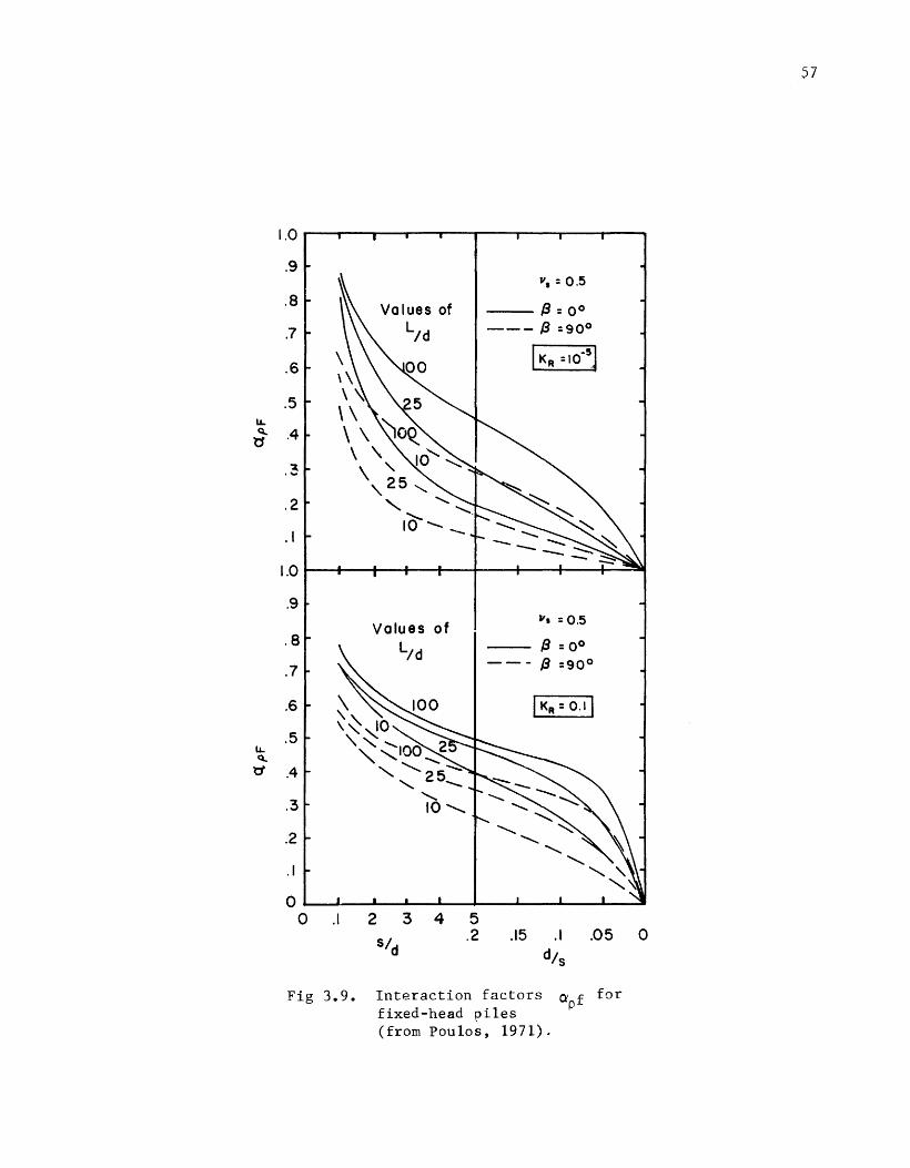
57
1.0
.9 "•: 0.5
.8 Values of 13: 0°
.7 L/d --- 13 =90°
.6 I KR =to-5J
.5 u. Q. .4 tt
.3
.2
.I
1.0
.9
Values of "• :0.5
.8 L/d -- /3 :QO
.7 ---13=90°
.6 I KR: 0.1,
.5 u. Q,
t:/ .4
.3
.2
.I
0 0 .I 2 3 4 5
S/d .2 .15 .I .05 0
dfs
Fig 3.9. Interaction factors Ctpf far fixed-head piles (from Poulos, 1971).
58
and
yG 3.93 X 10⁻⁶
[0.51(9150) + 9150]
= 0.054 in.
Using modified p-y curves, COM623 is employed to generate a curve showing
groundline deflection versus they-multiplier (Step 11, Fig 3.10). A multi-
plier is then selected which gives the same deflection as the deflection found
in Step 10 (Step 12).
Using this modifier, a solution is made with COM623. The results of this
solution (Step 13) are given in Fig 3.11. The final step is to check the
structural adequacy of the shaft.
The solution that was just presented indicated that the deflection com
puted by the p-y method was less than that computed by the Poulos elastic
method. Such a result is an anamoly because the p-y approach should represent
the "true" behavior of the pile. The conclusion would then be that the
elastic modulus that was selected for the soil for use in the Poulos method
was too low. However, for this particular solution the Poulos solution was
assumed to be correct for purposes of completing the solution.
As shown in Fig 3.11, the deflection is certainly tolerable. The maximum
bending moment of 63 k-ft results in a bending stress of 285 lb/in.2
.
Therefore, the design that is presented is conservative from the standpoint of
bending moment.
The Focht-Koch-Poulos procedure is rational and is being employed widely
at the present time. However, it is unproven by having been compared with a
sufficient number of results from prototype tests in the field to allow a
judgement to be made about the validity of the method. The few comparisons
that have been made (unpublished) show that the Focht-Koch-Poulos method gives
reasonable agreement with experimental results.
The next step in checking the design shown in Fig 3.7 is to check the
adequacy of the design under the axial loads that are shown.

..... cu
5.0
a. 4.0
I
>-
3.0
59
.. ----
1.054
.04 .05 .06
Ys, in.
Fig 3.10. Selection of p-y curve modifier.

-.... .. )( .. .r:. -0. Cl)
0
5
10
15
20
25
(a)
..
Deflection, y , in.
.05
-
(b)
Moment, ft K
10 20 30
1ft= 0.3048 m; 1000 lb/ft2 = 47.88 MPa; 1 ft-k = 1.356 kNm
Fig 3.11. Equivalent shaft deflections and moments for example problem for double-shaft group.
CQ= 1728 lb/ft2
Y=IIO lb/ft3
Dio=2.5 ft
L =25 .. 0 ft
Fixed Head
0'-0

61
INTERACTION OF CLOSELY SPACED SHAFTS UNDER AXIAL LOAD
In the preceding pages, methods of analysis and design have been outlined
for axial loading of single shafts and for the lateral loading of shaft
groups. The procedure fer lateral loading accounted for the interaction
between shafts in the group. The following discussion will treat the problem
of such interaction due to axial loading.
Poulos presents methods of analysis for a two-pile grouping (Refs 8
and 11). His methods, based upon theories of elasticity, treat the problems
of axial capacity and settlement. His methods must be recognized as approxi
mate, but give results that improve the ability of the designer to make
reasonable decisions.
Axial Deflection
For a two-shaft grouping, as has been mentioned previously, one shaft
will be subjected to tensile loads while the other will be subjected to com
pressive loads. The movements involved under these two types of loading will
be opposite in direction. Poulos gives the following expression for the
shaft-head displacement of a shaft under axial loading:
Pxil (3.19) Pa E d
s
where
p = applied axial load, X
Il an influence factor,
E Young's modulus of ilie soil, and s
d = shaft diameter.
I1
is a factor that is a function of pile or shaft diameter, base
diameter, and length. Figure 3.12 (from Poulos) gives values of I 1 • As
shown in Fig 3.13, Poulos also gives values of an a factor for the computa
tion of shaft interaction effects on axial movement where
= al settlement of shaft under its own load
additional settlement due to adjacent shaft (3.17)

62
1.0
d 0.8 1-
0
(.)
0 l.i...
c: 0 -0 0 1-Q) -c:
0.6
0.4
0.2
0 0
1.0 0.8 0.6
0.4
11 0.2 Values of db/d
0.1 0.08
0.06
0.04
0.02 0 10 20 30 40 50
L/d
Fig 3.12. Influence factor I 1 for axial
displacement (after Poulos, 1971).
___ , :0.5 ---11=0
2
s/d
Fig 3 .13. Interaction factor
I
IL IL
'1 1 1
_.,l,.._d --ill-- d ,._ s ----"1
0.1 d/s
for axial
displacement (after Poulos, 1971).
0

63
The curves of Fig 3.12 for r1
and Fig 3.13 for a1
allow an estimate
to be made of the interaction between drilled shafts supporting an overhead
sign. Figure 3.7 shows the typical loading for the two-shaft group. One load
tends to cause an upward movement as opposed to the downward movement of the
other shaft. This means that the "additional settlement" quantity should
actually be negative in value since the effect of the adjacent pile or shaft
is to cause movement opposite to the affected shaft movement.
As an illustrative example of the Poulos method, consider the two-shaft
system of Fig 3.7, with
L/d 10 1.0 where db diameter of shaft base.
From Fig 3 .12
0.15
(72,000 lb)(O.l5)
(3000 lb/in.2
)(30 in.)
= 0.12 inch
From Fig 3.13, with L/d 10 and s/d = 3 ' = 0.45
However, as pointed out, this value should be negative in value.
With this value of a1
, the movement of either shaft may be computed and
is
P + alp X X
0.12 + (-0.45)(0.12)
0.066 inch
This result indicates that the axial movement of a shaft of the size used
for overhead signs is relatively small and in most cases may be ignored. The
second point of interest is that the total movement of either shaft in the
double-shaft system will be less than that of the single shaft.
64
Shaft Capacities
Interaction between two shafts will affect the axial capacities of the
shafts as well as the axial deflections. A qualitative examination of a two
shaft group will be presented. The problem should not be viewed as an exact
solution but will indicate the trend of the behavior to be expected.
Figure 3.14 presents a simplified view of a two-shaft system. A free
body of shaft A is taken to include the soil mass enclosed within a cylin
drical shape of radius S and length L • The average shear stress on the
outer face of this soil cylinder may be approximated by
'TBA 2 nSL (3. 19)
If this value is used as the average shear stress between the surface of
shaft Band the soil mass, then the upward load dee to the stresses induced by
the load at A is
( ndL)
(3. 20)
For the previously presented problem then, the effect of A on B could
be approximated as
=
(72,000 lb)(2.5 ft) 2(7.5 ft)
12,000 lb
Thus, the compressive load can be considered to be reduced by 12~000 lb as is
the tensile load.
This figure should not be viewed as exact. For example, the load due to
a compressive load at one shaft calculated using Eq 3.20 ignores the fact that
only a portion of the load will be felt as an induced shear stress since part
of the load will be carried by the shaft base. However, the ideas expressed

65
i px ~px
I ~ I I
I _J
A B
~ rc s --1 \
\
-$-I
.. Soi I Cy I i nder"
Fig 3.14. Free body of two-shaft system.

66
are intuitively sound and may be thought of as increasing the overall factor
of safety of the system.
The methods presented in the preceding pages for the analysis and design
of two-shaft systems are felt to be both easy to use and as accurate as is
presently possible. As in all areas of design, care should be used to under
stand the theories, the assumptions, and, in particular, the limitations
involved in the use of the presented procedures. A major portion of design
must be the exercise of experience and gcod judgement.

CHAPTER 4. DESIGN PROCEDURE USING COMPUTER-BASED METHODS OF ANALYSIS
PRESENT CAPABILITIES
With the advent of high-speed digital computers many engineering problems
which were formerly too complex mathematically or simply too tedious to solve
have become manageable. The problem of the laterally loaded pile or shaft was
one such problem. Computer programs, making use of the finite difference
approach, currently nake the solution of this problem relatively straight
forward. The programs COM622 and COM623 have been specifically developed to
generate the necessary solutions.
Input and output examples for COM622 have been reported in the literature
(Ref 15). In addition, a detailed report on the capabilities and input/output
formats for COM623 has been supplied to SDHPT (Ref 17). Some important
aspects of the latter program will be summarized at this point.
COMPUTER-BASED ANALYSIS
COM623 allows great flexibility in problem formulation on the part of the
design engineer. The input format makes variation possible in both the soil
and structural parameters. For instance, the moment of inertia can vary along
the length of the shaft, independently of all other variables. Likewise, soil
parameters, such as soil unit weight, undrained shear strength of clay, and
internal angle of friction, can be varied, thus allowing the designer to make
the model of the system as simple or as complex as desired or as the available
data allow.
In addition, the program is structured in such a manner as to make
multiple solutions both easy and practical. If a load-deflection curve is
desired, the simple addition of extra load-value cards at the end of the data
deck will ~ause the necessary output to be generated. Output can also be
manipulated to some degree to avoid generation of excess output information.
67
68
Instead of station by station values of moment and outer fiber stresses, any
number of stations can be omitted or the entire table can be deleted so that
only the maximum values are output in a summary table. As has been stated, a
most complete and informative guide has already been developed and is avail
able if further questions arise.
APPLICATION OF ANALYTICAL METHODS TO DESIGN
Within the context of design, the several methods of analysis previously
mentioned can be manipulated to achieve a design, although some are much more
easily manipulated than others. If only the crudest of approximations to the
best solution is desired, a closed-form solution of the differential equation
would suffice. However, this would of necessity be overly restrictive,
complex, and time consuming.
In direct contrast to a closed-form solution would be a design procedure
based on a computer analysis of the system. A design procedure has been for
mulated which attempts to capitalize on the computer's availability and speed.
This procedure will be outlined, using as an example problem the shaft and
basic parameters used earlier in the section on charts developed at SDHPT for
design of single shafts. A basic summary of the steps will be made and then
each step will be discussed using the example problem for illustration.
SUGGESTED DESIGN PROCEDURE
Single-Shaft System - COM623 Design Procedure
(1) Determine soil properties; select shaft properties and cross
section geometries.
(2) Compute shaft design moment:
(3) Estimate EI as E I c gr
M u
0M n
(4) Estimate shaft length, L , such that "long" pile action occurs
(i.e., two points of zero deflection occurring along the shaft)
(5) Using values from Steps 1, 3, and 4, and COM623, generate, for
a range of lateral loads, P , curves of t
(a) lateral load versus maximum shaft moment1
(b) lateral load versus groundline deflection,
M , and max
y . t

(6)
(7)
(8)
With a value of M from Step 2, u enter Sa and find the
allowable load, p t a
With pt enter Sb to a
(a) insure that yt is not in the "critical" area of the
curve, and
(b) check yt for esthetic criteria, if any.
With p t a
and COM623, generate a versus L curve by
decreasing L until yt begins to increase significantly.
Choose a design length, L .
(9) Using PMEI (Appendix) or a similar program, generate a moment
versus EI curve. Refine the estimate of EI , if deemed
necessary, and rerun COM623 with new EI values.
(10) Check results of Step 9 for unacceptable changes in yt or
M max
EXAMPLE PROBLEM
69
The first stage of the procedure involves the collection and evaluation
of all pertinent design data. Design solutions, in the end, are limited by
design input and, therefore, every effort should be made to identify and
select appropriate values. For purposes of illustration, certain parameters
used here have been simplified.
The soil deposit is input as a homogeneous, single-layer, clay deposit.
Shear strength, unit weight, and €SO are assumed constant with depth and
equal to 1728 lb/ft2 , 115 lb/ft3 and 0.010 respectively (Fig 4.1). The water
table is below the shaft base and the initial modulus of subgrade reaction,
k , is equal to 5.0 x 10⁵ lb/ft3 . Loading is chosen to be cyclic in nature. s
It should be mentioned that it is usual for most of these parameters to be
unavailable to the design engineer. However, values that will provide a
sufficient order of accuracy can be obtained from many different sources in
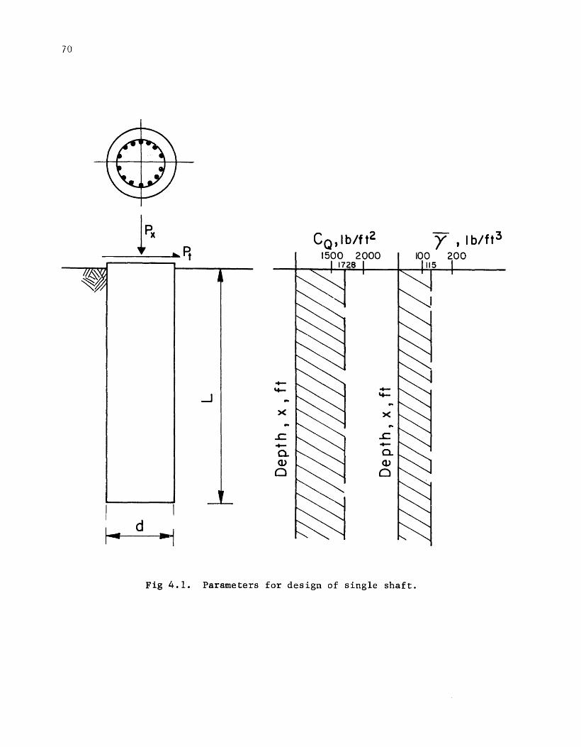
70
I
I~ d
,, I
--i
)(
..c +-c.. OJ
0
c0 , lb/tt2
1500 2000 1728
Fig 4.1. Parameters for design of single shaft.
y , lb/ft3
100 200 115

71
the literature when necessary. The engineer's judgment and experience, as in
all other design processes, may also be called upon.
If there are no limits set upon shaft geometries, a trial section must be
formulated. In many instances, certain limits, as to diameters and reinforce
ment arrangements, are in effect and must be observed. At SDHPT, certain sizes
are more frequently used than others and a natural preference seems to have
evolved for a 30-inch~diameter shaft. For this problem, a 30-inch-diameter
shaft has been chosen with a circular pattern of 14 II 11 bars (p = 3.1
percent) enclosed with a 113 spiral. Concrete is designated as Class A with a
28-day strength of 3000 lb/in.2
and the reinforcing steel is Grade 60
(ultimate strength is 60,000 lb/in. 2 ).
With the basic soil and shaft parameters established, St~p 2 is
performed. Several programs exist, or are in the process of being written,
for computing the design moment of a circular section. Simpler versions for
use with hand-held programmable calculators are also being developed, although
such an approach of necessity requires some manual bookkeeping. ACI design
handbooks can also be used to obtain the desired value.
Step 3 involves the estimation and computation of the shaft's stiffness.
The modulus of elasticity can be computed using the ACI 318-77 formula for
normal weight concrete:
E c
57,000 f 1 1/2 c
(4 .1)
The moment of inertia of the cross section can be computed in one of several
ways. The small reinforcing can be transformed to an equivalent concrete area
and consideration can be given to the effects of cracking. However, as has
been mentioned, the product EI has a relatively small effect on the
behavior of the system. For this reason, the moment of inertia used in this
problem is the gross moment of inertia. It is felt that most design problems
will be of such a nature that this gross value will be adequate and no further
refinement is needed.
The next part of the procedure involves the estimation of an initial
shaft length that will insure that "long pile" action occurs. This could be
any value desired and is used only as a guide to the rest of the design
process. For this example a length of 40 feet was selected. This length can
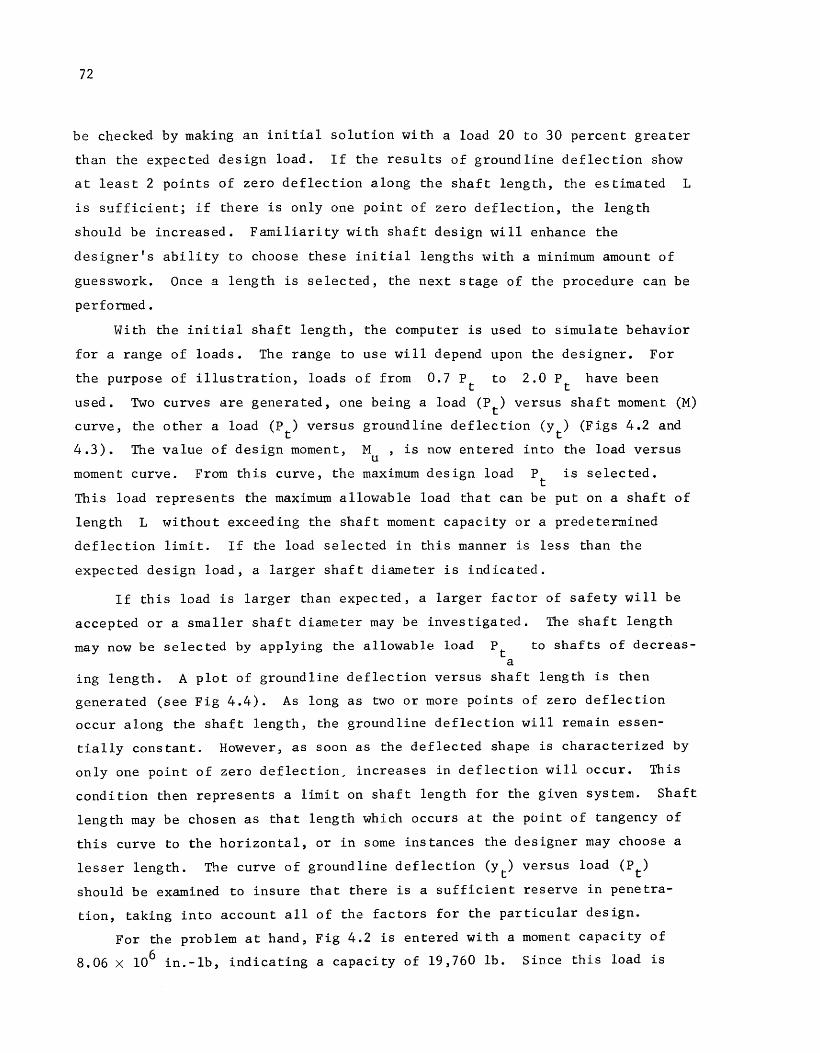
72
be checked by making an initial solution with a load 20 to 30 percent greater
than the expected design load. If the results of groundline deflection show
at least 2 points of zero deflection along the shaft length, the estimated L
is sufficient; if there is only one point of zero deflection, the length
should be increased. Familiarity with shaft design will enhance the
designer's ability to choose these initial lengths with a minimum amount of
guesswork. Once a length is selected, the next stage of the procedure can be
performed.
With the initial shaft length, the computer is used to simulate behavior
for a range of loads. The range to use will depend upon the designer. For
the purpose of illustration, loads of from 0.7 Pt to 2.0 Pt have been
used. Two curves are generated, one being a load (Pt) versus shaft moment (M)
curve, the other a load (P ) versus groundline deflection (y ) (Figs 4.2 and t t
4.3). The value of design moment, M , is now entered into the load versus u
moment curve. From this curve, the maximum design load Pt is selected.
This load represents the maximum allowable load that can be put on a shaft of
length L without exceeding the shaft moment capacity or a predetermined
deflection limit. If the load selected in this manner is less than the
expected design load, a larger shaft diameter is indicated.
If this load is larger than expected, a larger factor of safety will be
accepted or a smaller shaft diameter may be investigated. The shaft length
may now be selected by applying the allowable load Pt to shafts of decreas-a
ing length. A plot of groundline deflection versus shaft length is then
generated (see Fig 4.4). As long as two or more points of zero deflection
occur along the shaft length, the groundline deflection will remain essen
tially constant. However, as soon as the deflected shape is characterized by
only one point of zero deflection, increases in deflection will occur. This
condition then represents a limit on shaft length for the given system. Shaft
length may be chosen as that length which occurs at the point of tangency of
this curve to the horizontal, or in some instances the designer may choose a
lesser length. The curve of groundline deflection (yt) versus load (Pt)
should be examined to insure that there is a sufficient reserve in penetra
tion, taking into account all of the factors for the particular design.
For the problem at hand, Fig 4.2 is entered with a moment capacity of
8.06 x 106 in.-lb, indicating a capacity of 19,760 lb. Since this load is

73
CQ = 1728 lb/ft2
2.0 Dia =2.5ft. • C y c li c Load l no • 2 0 c y c I e s I Pt = 18,300 lb
1.9 •
/ 1.8 •
I 1.7 •
I 1.6 •
I 1.5 • - I a..
"0 1.4 a
0 I 0 ..J
1.3 • 0 I '-Cl.l - 1.2 • c
I ..J
1.1 • 1.0 8 p t -;1
1.0
cg I •
I .8 • 8.06 X 10 6
I .7 4 5 6 7 8 9 10 II 12 13 14 15
Shaft Moment, M, in. -lb x 106
Fig 4o2. Shaft moment versus lateral load.

74
.. Q. .. "tJ c 0 ~
c '-Q,) -c _J
1.9
1.8
1.7
1.6
1.5
1.4
1.3 I •
I 1.2 •
I •
1.08~
I· •
I
1.1
.9
.8 •
•
I •
I •
I •
•
I •
I
•
I
c0 = 1728 lb/ft2
Dio = 2.5 ft.
Cyc lie Load ino = 20 cycles
p t = 18,300 lb
I .7 --------~~------~---------+--------~--------~~
1.0 2.0 3.0 4.0
Groundline Deflection,yt,in.
Fig 4.3. Groundline deflection versus lateral load.

c -.. ->-.. c 0 ·--u Q) -.... Q)
0
Q)
c ·--"0 c ::J 0 '-~
•
6.0
5.0' •
4.0
3.0
2.0
1.0
.\ ·~
c0 =1728 lb/ft 2
Dia=-2.5ft
C y c I i c Loading = 2 0 c y c I e s
Pt =18,300 lb
Arrow indicates Approximate Length at which "Long Pile"
Action occurs
."" + • • ·---- -- . _-............-. ----=-·---=-·- - ·----·+· 0 1ss-17~~~~~--~=:~~~--~~l--+--+-~--~--+--+--~~~~ I 17 18 19 20 25
Shaft Embedment Length , L , f t 30
Fig 4.4. Groundline deflection versus embedment length of shaft. -......! I.Jl
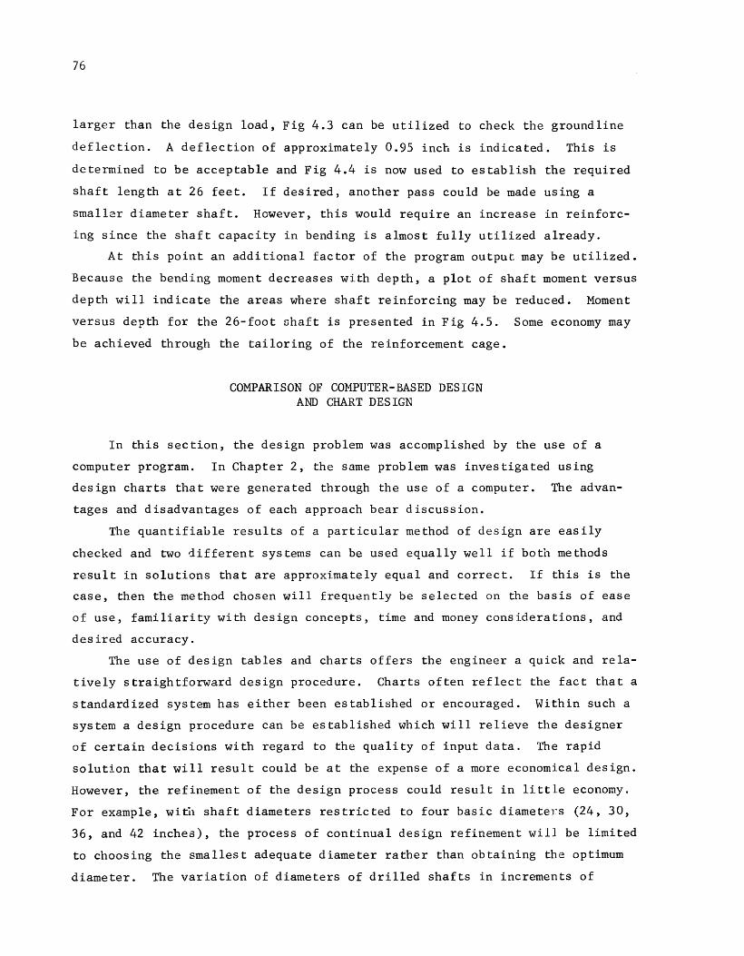
76
larger than the design load, Fig 4.3 can be utilized to check the groundline
deflection. A deflection of approximately 0.95 inch is indicated. This is
determined to be acceptable and Fig 4.4 is now used to establish the required
shaft length at 26 feet. If desired, another pass could be made using a
smallzr diameter shaft. However, this would require an increase in reinforc
ing since the shaft capacity in bending is almost fully utilized already.
At this point an additional factor of the program output may be utilized.
Because the bending moment decreases with depth, a plot of shaft moment versus
depth will indicate the areas where shaft reinforcing may be reduced. Moment
versus depth for the 26-foot shaft is presented in Fig 4.5. Some economy may
be achieved through the tailoring of the reinforcement cage.
COMPARISON OF COMPUTER-BASED DESIGN AND CHART DESIGN
In this section, the design problem was accomplished by the use of a
computer program. In Chapter 2, the same problem was investigated using
design charts that were generated through the use of a computer. The advan
tages and disadvantages of each approach bear discussion.
The quantifiable results of a particular method of design are easily
checked and two different systems can be used equally well if both methods
result in solutions that are approximately equal and correct. If this is the
case, then the method chosen will frequently be selected on the basis of ease
of use, familiarity with design concepts, time and money considerations, and
desired accuracy.
The use of design tables and charts offers the engineer a quick and rela
tively straightforward design procedure. Charts often reflect the fact that a
standardized system has either been established or encouraged. Within such a
system a design procedure can be established which will relieve the designer
of certain decisions with regard to the quality of input data. The rapid
solution that will result could be at the expense of a more economical design.
However, the refinement of the design process could result in little economy.
For example, witi1 shaft diameters restricted to four basic diameters (24, 30,
36, and 42 inches), the process of continual design refinement will be limited
to choosing the smallest adequate diameter rather than obtaining the optimum
diameter. The variation of diameters of drilled shafts in increments of

2
4
6
8
10
- 12 .... )( .. 14 &. -0.
16 cu 0
18
20
22
24
26
28
Shaft Moment, M, in.-lb x 106
1.0 2.0 3.0 4.0 5.0 6.0 7.0 8.0
• /
• /
• /
• I
/.
\ \ • J • j
I
ca = 112 8 lb/tt 2
Dia = 2.5 ft Cyclic Loading= 20cycles
Pt = 18 ,300 lb
Fig 4.5. Bending moment in shaft versus depth.
77
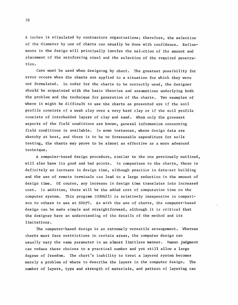
78
6 inches is stipulated by contractors organizations; therefore, the selection
of the diameter by use of charts can usually be done with confidence. Refine
ments in the design will principally involve the sel,=ction of the amount and
placement of the reinforcing steel and the selection of the required penetra
tion.
Care must be used when designing by chart. The greatest possibility for
error occurs when the charts are applied to a situation for which they were
not formulated. In order for the charts to be correctly used, the designer
should be acquainted with the basic theories and assumptions underlying both
the problem and the technique for generation of the charts. Two examples of
where it might be difficult to use the charts as presented are if the soil
profile consists of a weak clay over a very hard clay or if the soil profile
consists of interbedded layers of clay and sand. When only the grossest
aspects of the field conditions are known, general information concerning
field conditions is available. In some instances, where design data are
sketchy at best, and there is to be no foreseeable expenditure for soils
testing, the charts may prove to be almost as effective as a more advanced
technique.
A computer-based design procedure, similar to the one previously outlined,
will also have its good and bad points. In comparison to the charts, there is
definitely an increase in design time, although practice in data-set building
and the use of remote terminals can lead to a large reduction in the amount of
design time. Of course, any increase in design time translates into increased
cost. In addition, there will be the added cost of computation time on the
computer system. This program (COM623) is relatively inexpensive in compari
son to others in use at SDHPT. As with the use of charts, the computer-based
design can be made simple and straightforward, although it is critical that
the designer have an understanding of the details of the method and its
limitations.
The computer-based design is an extremely versatile arrangement. Whereas
charts must face restrictions in certain areas, the computer design can
usually vary the same parameter in an almost limitless manner. Human judgment
can reduce these choices to a practical number and yet still allow a large
degree of freedom. The chart's inability to treat a layered system becomes
merely a problem of where to describe the layers in the computer design. The
number of layers, type and strength of materials, and pattern of layering can

79
all be easily input and a whole series of structural variations can be examined
in a very short period of time. Another aspect of the computer-based design
is the production of not only a final size but also a complete description of
the behavior of the soil-structure system.

!!!!!!!!!!!!!!!!!!!"#$%!&'()!*)&+',)%!'-!$-.)-.$/-'++0!1+'-2!&'()!$-!.#)!/*$($-'+3!
44!5"6!7$1*'*0!8$($.$9'.$/-!")':!

CHAPTER 5. GENERATION OF DESIGN AIDS
Design aids such as the ones developed by the Texas State Department of
Highways and Public Transportation are popular for a variety of reasons. In
many instances they provide design solutions that are safe and economical, and
the aids are relatively easy to use. Situations are often such that highly
exact, theoretical solutions are no better than less rigorous, approximate
solutions, simply because the designer is unable to obtain accurate and reli
able data for input. Where this is the case, design aids based upon simpli
fying assumptions and generalization of certain parameters will provide
adequate solutions. However, the aids must be formulated using sound theory,
and the limitations and generalizations used must be fully understood by both
the author of the aids and the user.
For example, tables and curves generated using soil properties such as
shear strength or unit weight that are constant with depth should not be
expected to give more than approximate design in cases where extensive explor
ations indicate that a complex, layered system exists. In such an instance
design aids would best be used as a point of departure in a more detailed
process. Conversely, many soil profiles show somewhat constant character
istics, and designs in such instances can be adequately made using the appro
priate tables and curves.
GENERATION PROCEDURE
The generation of design aids can be accomplished with the aid of COM623.
The process can be approached in several different ways, with no single
approach being essential. Certain generalizations peculiar to one approach
may or may not be made in another. One such method of generation is discussed
below.
81
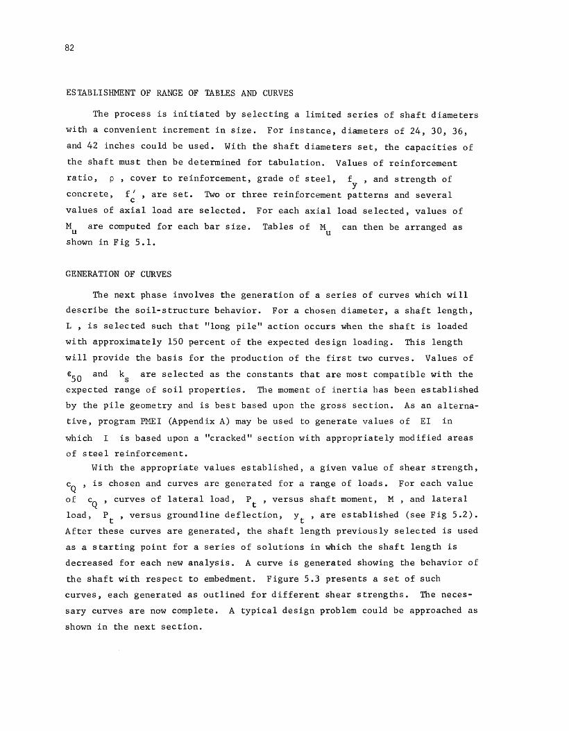
82
ESTABLISHMENT OF RANGE OF TABLES AND CURVES
The process is initiated by selecting a limited series of shaft diameters
with a convenient increment in size. For instance, diameters of 24, 30, 36,
and 42 inches could be used. With the shaft diameters set, the capacities of
the shaft must then be determined for tabulation. Values of reinforcement
ratio, p , cover to reinforcement, grade of steel, f , and strength of y
concrete, f' are set. Two or three reinforcement patterns and several c '
values of axial load are selected. For each axial load selected, values of
M are computed for each bar size. Tables of M can then be arranged as u u
shown in Fig 5.1.
GENERATION OF CURVES
The next phase involves the generation of a series of curves which will
describe the soil-structure behavior. For a chosen diameter, a shaft length,
L , is selected such that "long pile" action occurs when the shaft is loaded
with approximately 150 percent of the expected design loading. This length
will provide the basis for the production of the first two curves. Values of
e50 and ks are selected as the constants that are most compatible with the
expected range of soil properties. The moment of inertia has been established
by the pile geometry and is best based upon the gross section. As an alterna
tive, program PMEI (Appendix A) may be used to generate values of EI in
which I is based upon a "cracked" section with appropriately modified areas
of steel reinforcement.
With the appropriate values established, a given value of shear strength,
cQ , is chosen and
of cQ , curves of
load, Pt , versus
curves are generated for a
lateral load, p t ' versus
groundline deflection, yt
range of loads. For each value
shaft moment, M '
and lateral
' are established (see Fig 5.2).
After these curves are generated, the shaft length previously selected is used
as a starting point for a series of solutions in which the shaft length is
decreased for each new analysis. A curve is generated showing the behavior of
the shaft with respect to embedment. Figure 5.3 presents a set of such
curves, each generated as outlined for different shear strengths. The neces
sary curves are now complete. A typical design problem could be approached as
shown in the next section.

83
p = 0 k X
# of Bars/M ; Shaft Diameter, in. Notes u Values of Moment
in ft-k 30 36 42 Based on p = 0 k X
9 8/375'k 10/591 14/1006 f I = 3.6 ksi c
f = 60.0 ksi 10 6/349 8/593 12/1078 y
p ~ 1.0 percent
11 -1 - 6/541 10/1116 2.25-in. cover (clear) to if 3 spiral (6-in. pitch)
p = 500 k X
if of Bars/M u ; Shaft Diameter, in. Notes
Values of Moment in ft-k 30 36 42 Based on p = 500 k
X
8/536-;'( 10/858 14/1228 f I = 3.6 ksi
9 c
f = 60.0 ksi 10 6/520 8/854 12/1267 y
p ~ 1.0 percent
11 -1 - 6/840 10/1286 2.25-in. (clear) cover to 1ft 3 spiral (6- in. pitch)
p = 1000 k X
iF of Bars/M ; Shaft Diameter, in. Notes u
Values of Moment in ft-k 30 36 42 Based on p = 1000 k
X
f I = 3. 6 ksi 9 8/483* 10/904 14/1448 c
f = 60.0 ksi 10 6/470 8/901 12/1489
y
p ~ 1.0 percent
11 -1 - 6/874 10/1500 2.25-in. cover (clear) to iF 3 spiral (6-in. pitch)
1ft= 0.3048 m; 1 ft-k = 1.356 kN-m; 1000 lb/ft2
= 47.88 MPa;
1000 lb = 0.4536 Mg
Fig 5.1. Tables of ultimate moment.
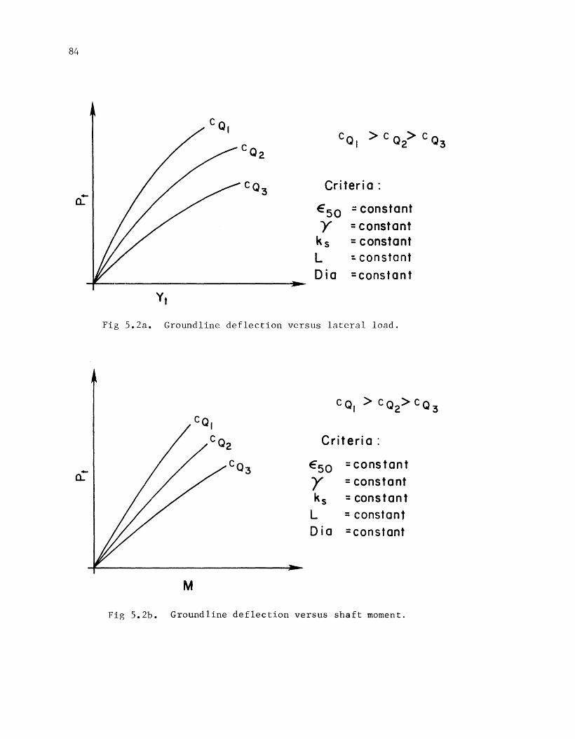
84
-c... Criteria:
E' 50 =constant Y =constant
k s =constant L :. constant Dia =constant
Fig 5.2a. Groundline deflection versus lateral load.
M
Criteria:
Eso y ks
L
=constant =constant =constant = constant
D i a =constant
Fig 5.2b. Groundline deflection versus shaft moment.

->-
L
ca >ca >ca I 2 3
Criteria·.
=constant =constant =constant =constant =constant
Fig 5.3. Groundline deflection versus shaft length.
85

86
USE OF TABLES AND CURVES
All available data are examined and values of shear strength, unit
weight, and soil type are selected. A trial diameter and reinforcement
pattern is selected for the given design loads. With a value of
enter the Pt versus M chart and find the shaft moment, M p t '
Check the
table to ensure that the capacity of the cross section is not exceeded. M u
If the shaft moment is less than the cross section capacity, the next step is
to enter the Pt versus yt chart. If the shaft moment is greater than the
section capacity, a large diameter should be chosen. Once the chosen section
checks as adequate the deflections may be checked.
With the design load, Pt , and the Pt versus yt charts, the deflec
tions may be determined. If these appear to be less than the allowable, the
procedure continues; if not, a larger diameter must be chosen. The shaft
length can be set once the deflection criteria have been satisfied.
versus L chart will give the design length by any method desired.
The
When
generating these curves, care should be taken to mark each curve with the
length at which pile behavior changes from that of having two points of zero
deflection to that of having only one point. This can be used as a reference
point in selecting a design length. Another method, giving slightly shorter
lengths, would be to lay a straight edge along the straight (horizontal)
portion of the appropriate curve and determine the point of tangency to the
curved segment. This could then be the chosen design length. As a third
option, a value of deflection could be predetermined. The curves could then
be entered with this value and a corresponding length chosen. This procedure
would, however, ignore the beneficial behavior of the longer pile in resisting
load and overload.
The design aids are limited by several factors and earlier sections
discuss the restrictions inherent in such design aids. With this in mind, the
method can be used to find a preliminary design and a final design when the
particular design warrants such an approach.
The brief presentation in this section provides no guidance for integra
ting the tables and curves into a series of charts, tables, curves, or noma
graphs. Such integration is, of course, possible. A possible approach would
be to develop the required number of tables and families of curves as illus
trated and to present them in a manual with appropriate indexing.
CHAPTER 6. SAN ANTONIO TEST AND RESULTS
In December 1978 and January 1979, two sets of drilled-shaft foundations
were made available by SDHPT for testing. The shafts were located on the
western section of IH 410 in San Antonio, Texas. They had been in use as
foundations for an overhead-sign structure that spanned the southbound lane.
The existing signing and supports were to be moved to another position and the
shaft foundations removed to allow the construction of a new access roadway.
The major portions of the shafts were to remain in the ground with only the
top several feet being removed and the holes backfilled. Because the shafts
were of no further use, testing to failure was permissible. The vertical-
support trusses were available for use in the testing. However, they were to
be reused and could not be damaged during testing. Furthermore, analysis
seemed to indicate that the anchor bolts in the heads of the shafts could not
withstand the loads that were expected to be applied in order to cause shaft
failure. For these reasons, it was decided not to use the vertical trusses or
the anchor bolts for purposes of load application. This decision ruled out
the possibility of loading the shaft at some point above the shaft head (a
loading which would produce both shear and moment at the top of the shaft).
It was decided instead to test the shaft by applying the load at the top of
the shaft.
TEST SITE AND CONDITIONS
The aims of the testing program in San Antonio were as follows: to
obtain data by which the analytical procedures could be evaluated, to obtain a
direct indication of the strength of a drilled shaft in a typical installa
tion, and to obtain physical evidence concerning the interaction of a drilled
shaft with the supporting soil.
The two test sites were near the intersection of U.S. 90 and IH 410 in
west San Antonio. The sign structure had spanned the southbound lane, with
one set of foundations located between the northbound and southbound main
87

88
lanes and the other set located between the southbound main lane and a
southbound feeder road (see Fig 6.1). The latter set was designated Site 1
for further discussion, with the shafts between the north and southbound main
lanes as Site 2.
Site 1 lay within a drainage ditch that sloped up to the south (see
Fig 6.2a). It can be assumed that some cut and fill took place in the area,
for construction of the roadways, with the entire area resodded after con
struction. Site 2 was somewhat different in that, instead of resodding, a
base coat of crushed rock about 6 inches thick and covered by an inch of
asphaltic material was placed after the road and drainage ditch had been
graded. It can be assumed that the soil in the first few feet had undergone
considerable compaction relative to the Site 1 material. Figures 6.2a
and 6.2b give detailed layouts of both sites.
The test at Site 1 was performed on December 15, 1978, and the test at
Site 2 on January 31, 1979. In both cases, the testing was carried out imme
diately following the passing of a weather front from the north. The weather
was therefore dry and cold with some gusting northerly winds and clear skies.
However, due to the passing of the storm, the soil at Site 1 was fairly well
saturated and soft enough for a small utility van to become stuck near the
site.
Soils testing was performed at Site 1 in July 1978. This was done
immediately after a period of severe rains and the ground was extremely soft.
An SDHPT drilling rig was used to obtain 3-inch "undisturbed" samples as well
as to perform the SDHPT pen test. The samples were tested at the site with a
pocket penetrometer and pocket torvane device. Q-type triaxial tests were
performed in the laboratory at The University of Texas at Austin. The results
of these tests are given in Fig 6.3. It is to be noted that the soil was
badly fissured and that the fissures opened very quickly after being extruded
from the sampling tubes, making trimming and testing difficult.
TEST DETAILS
SHAFT CONFIGURATION
As mentioned previously, Site 1 was located within a drainage ditch which
had been resodded after construction. The point of load application to the
shafts was to be at the shaft head. Because of the shaft positions it was

N
@
1 ft 0.3048 m
Q)• 0
-~I '- .
Plan View OSB A45 06 Sto. 38+ 31 Urban
Loop 410 West at US Hwy 90 San Antonio. Tex.
Scale 111 = 20•
June 27,1978
Steel Beam Guard Roil -IO"Dia. Wood Posts 6' O.C., 2.5' High
89
3t8 .. 'Wire Rope -Steel Posts 25·o.c, 2.5 I High
Southbound Lones
Loop 410 West
40 I
Site I
Test Site 2
2.31
Fig 6.1. San Antonio test site.

90
Grout Pad
Drilled Shafts
2.5' Dia.
Grout Pad
~ N
1 ft = 0.3048 m
Steel Guard Rail
(.}
• (.)
10
Traf fie Signal Box -
~
~ _l I \__TBM Elev =98.4•
2.31
2.41 1.9 I
Fig 6.2a. San Antonio test site 1.

t. f------13-15' .. j ..
Southbound
Lane,
Loop 410
Edge of Pavement
1 ft 0.3048 m
Guard Rail/---:;:o-
. / v Grout Pad
30.. I I Drilled Shaft..:....._......,.
: I I 1 Grout 1 Pad
I 2• 1 .. .. .
13-151
Guard
R~ _;-
(_) I
(_)
Fig 6.2b. San Antonio test site 2.
91
N
@
-1 Edge of Pavement
/
Northbound Lane,
Loop 410

10+
- I ~ . )( .
.s:::. I -0. cu 0 I
2J
'
Blow Count, N, SDHPT Pen-test Shear Strength, Ca • P.S. F.
50 100 500 1000 2000
0 0
(11) •
0 (18)
U T Tri-oxio I I \ '\ Lob. Test
0(23)
I • SDHPT-THD Pen Test Correlation
0 I oUT Triaxial Test (25)
1ft= 0.3048 m; 1000 lb/ft2 = 47.88 MPa
Fig 6.3. Soils test results.
\.0 N

93
felt that the application of load between the two shafts would be acceptable.
The size of the jacking equipment dictated that an inch or so of soil be
removed in areas near the southernmost shaft. Site 2 presented a similar
problem. The tops of the shafts were located 2 to 3 inches above the asphalt,
necessitating the removal of 6 to 8 inches of material. This material was
also removed for a distance of 3 to 4 inches all around the shafts at Site 2
in an attempt to keep the increased stiffness of the base and asphaltic
materials from influencing the test results.
The shafts for both sites were straight-sided 30-inch-diameter shafts
spaced 6.0 feet center to center. The lengths were specified on the original
plans to be 17 teet at Sites 1 and 2. However, there was no way to verify the
embedment. The ground surface around the shaft heads varied from being almost
level with the shaft head to being as much as 6 to 8 inches below the shaft
head. At both sites, minor excavation was performed between shafts to allow
room for the jacking system. At Site 1 a guard rail was located approximately
2-1/2 feet to the west of the shafts. Site 2 had guard rails located on both
sides of the shafts.
LOAD SYSTEM
The load system consisted of a hydraulic ram, "saddle" blocks, spacers, a
load cell, and a swivel joint (Fig 6.4). The saddle blocks were constructed
of steel plate and were cushioned on the shaft faces by neoprene pads. The
hydraulic ram was a double-acting ram of 60 kips capacity (Site 1) and 100
kips capacity (Site 2), each with 10-inch strokes. The spacers were two round
steel pipes 2-1/2 inches in diameter with 1/2-inch-thick walls and approxi
mately 4 and 6 inches in length. The swivel consisted of 2 cylindrical steel
shapes, each having one face dished out. A hardened steel ball was placed
between the two pieces, allowing the loading system to pivot about a point as
the two shaft faces rotated from the vertical. The ram was powered by a
hydraulic pump. Pressures were regulated by a system of valves to attain
predetermined strain readings from the load cell.
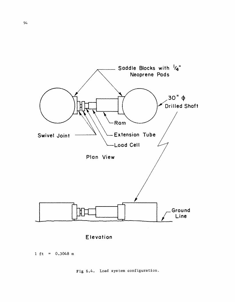
94
Swivel Joint
1 ft = 0.3048 m
Saddle Blocks with 114 ..
Neoprene Pads
30 II 4> /orilled Shaft
\_Ram Extension Tube
Load Cell
Plan View
Elevation
Fig 6.4. Load system configuration.
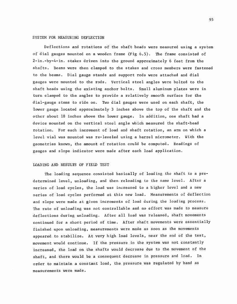
95
SYSTEM FOR MEASURING DEFLECTION
Deflections and rotations of the shaft heads were measured using a system
of dial gauges mounted on a wooden frame (Fig 6.5). The frame consisted of
2-in.-by-4-in. stakes driven into the ground approximately 6 feet from the
shafts. Beams were then clamped to the stakes and cross members were fastened
to the beams. Dial gauge stands and support rods were attached and dial
gauges were mounted to the rods. Vertical steel angles were bolted to the
shaft heads using the existing anchor bolts. Small aluminum plates were in
turn clamped to the angles to provide a relatively smooth surface for the
dial-gauge stems to ride on. Two dial gauges were used on each shaft, the
lower gauge located approximately 3 inches above the top of the shaft and the
other about 18 inches above the lower gauge. In addition, one shaft had a
device mounted on the vertical steel angle which measured the shaft-head
rotation. For each increment of load and shaft rotation, an arm on which a
level vial was mounted was re-leveled using a barrel micrometer. With the
geometries known, the amount of rotation could be computed. Readings of
gauges and slope indicator were made after each load application.
LOADING AND RESULTS OF FIELD TEST
The loading sequence consisted basically of loading the shaft to a pre
determined level, unloading, and then reloading to the same level. After a
series of load cycles, the load was increased to a higher level and a new
series of load cycles performed at this new load. Measurements of deflection
and slope were made at given increments of load during the loading process.
The rate of unloading was not controllable and no effort was made to measure
deflections during unloading. After all load was released, shaft movements
continued for a short period of time. After shaft movements were essentially
finished upon unloading, measurements were made as soon as the movements
appeared to stabilize. At very high load levels, near the end of the test,
movement would continue. If the pressure in the system was not constantly
increased, the load on the shafts would decrease due to the movement of the
shaft, and there would be a consequent decrease in pressure and load. In
order to maintain a constant load, the pressure was regulated by hand as
measurements were made.

Existing Anchor Bolts
(Ty p .)
Slope
1 ft = 0.3048 m
u--
Dial Gage Supports (2x4)
Slope Indicator
/
Dial Gage
I
Dial --Gage
v---Dial Gage
,- -·-•---, I
Shafts
2 11X 10
11
2 x 2 Stakes
Main Beams Clamped to Stakes with 1211
.. C .. Clamps
Polished AI uminum Pads for Dial Gage Tip to Ride on
Ground Line
Fig 6.5. Deflection and slope measurement system configuration.
\D 0'

97
The results of the testing are presented in Figs 6.6, 6.7, and 6.8. The
capacities of the shafts were approximately the same for both sites. Loads of
from 60 k to 70 k caused behavior that could be interpreted as failure.
Within this load range the rate of deformation occurring did not seem to
decrease with time. When an attempt was made to increase the load, the
deflection rate would increase. Loading was continued until the system was
extended enough that an unstable configuration occurred at the swivel joint.
At Site 1 this represented a deflection of around 4 inches at each shaft; at
Site 2, around 2-1/2 inches for each shaft.
Figure 6.7 illustrates the effect of cyclic loading on deflections. For
each additional cycle of load the deflection increases with the increase being
larger at higher loads. Dashed lines indicate limits that could be expected
for static or cyclic loading. A static loading would follow the upper dashed
line. A cyclic loading would, for a given load value, produce a point on the
lower dashed line. In this manner the two lines may be thought of as upper
and lower limits on the shafts' behavior.
It was noted that at the conclusion of any given loading a certain amount
of permanent deformation existed. Figure 6.8 presents the residual or perma
nent deflections noted during the cycling of the 60-k load. Figure 6.9
illustrates the patterns of soil disturbance noted at the end of testing.
Semi-annular openings, on the order of 3/4 inch to 1-1/4 inch in width and
extending around the shaft for about 120°, were noted. At both sites these
openings occurred not at the shaft surface but at a distance of 2 to 3 inches
from the surface.
This indicates that the soil-structure interface remained intact and that
failure actually occurred within the soil mass. At Site 2 a meter stick was
inserted into the opening to a depth of 35 inches. At both sites radial
cracks in the soil surface were noted on the side opposite to the load appli
cation. A slight mounding of the soil was observed in this area. None of the
shafts indicated any distress in the concrete.
COMPARISON OF FIELD TEST RESULTS TO COMPUTER ANALYSES
An analysis was made using COM623 and all available data for the site.
The results are presented in Fig 6.10. If a shaft length corresponding to
that indicated on the plans is used, the results are quite conservative,
especially for higher load levels. Several different parameters can be varied
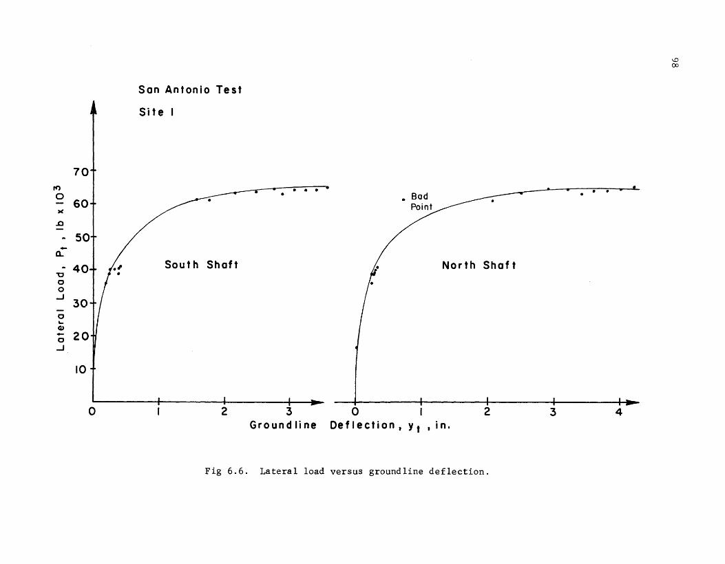
, I 0
60 ><
.c - .. -a..
I I
-~--.-- ... -"C c 0
...J 30 -c ~
Q)
; 20 ...J
10
0
Son Antonio Test
Site I
____..---.-----. . . . ~-""
______. .
South Shaft ;; North Shaft
2 3 0 2 Ground line De fIe c t ion , y t , in I
Fig 6.6. Lateral load versus groundline deflection.
- • •
3
.
4
1..0 00

10
en Q) -u >-u ,.._ 0
... 5 Q)
.0 r E ::J z
0
Son Antonio Test
Site I
60 kips Cycled
I
2
South
Shof t
3
/ /
North
Shaft
I I I I ... 0 I 2 3
Residual Groundline Deflection, y, in.
Fig 6.7. Lateral load versus groundline deflection. \0 1.0
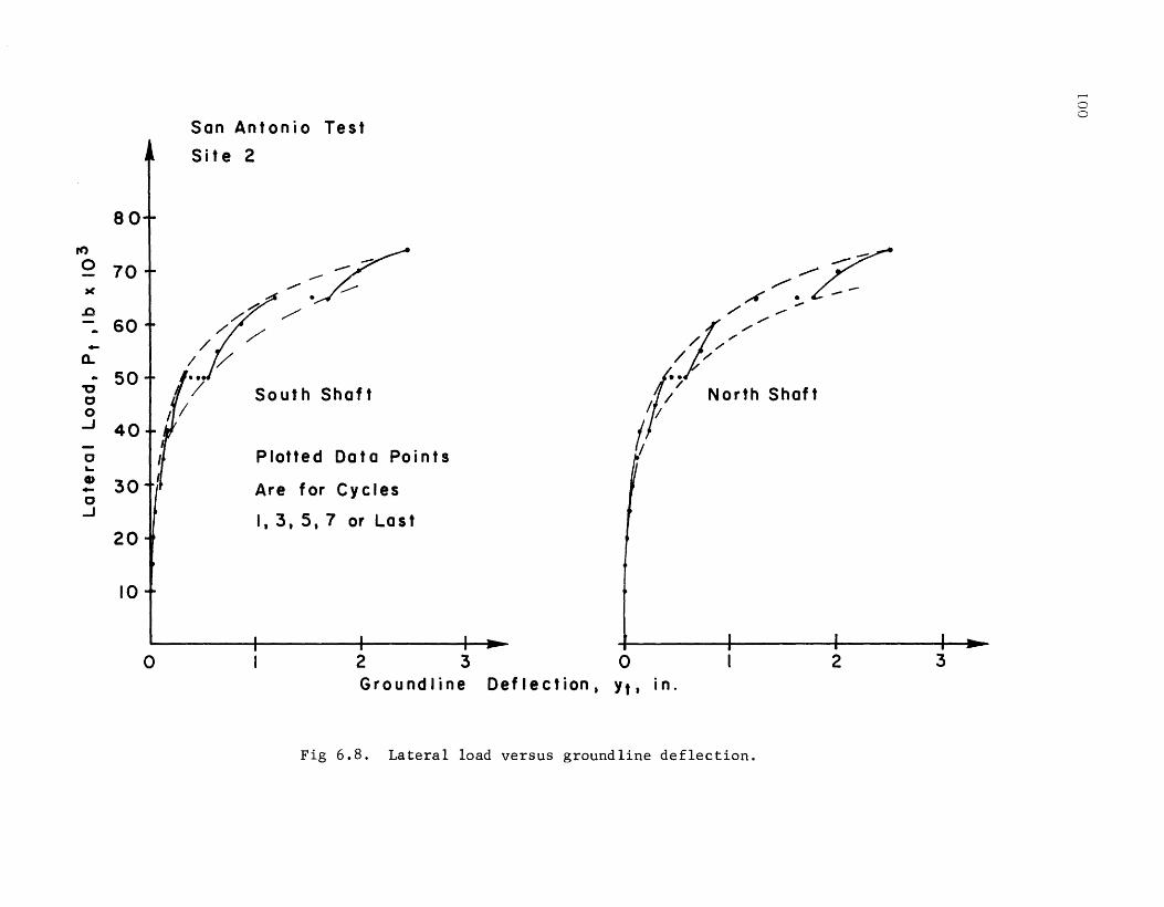
rt)
0
)(
.0
-a. .. "C 0 0 ..J
0 '-G) ... 0 _J
80
70
60
50
San Antonio Test
Site 2
~/ r/· / / /
/ ,....~
f/~,!-,"'
/ /
t·/ South Shof t I I
f" North Shaft
~ 40
1/1 Plotted Data Points
30 11' Are for Cycles
I, 3, 5, 7 or Last 20
10
0 2 3 0 2 Groundline Deflection, Yt• in.
Fig 6.8. Lateral load versus groundline deflection.
3
..........
0 0

A Semi -annular
Openings
D
Plan
Section A-A Site I
Semi-annular r- Openings
Plan
Section 8-8 Site 2
Fig 6.9. San Antonio test, observed failure patterns.
101
A
8

/ 50+ I
~ 401! ~ if!/. ~ 30 to&.
~ 20 {f
60
•
•
_J
10
0 3 4 5 6
Ground I i ne Deflection , Y t , in.
1 ft = 0.3048 m; 1000 lb = 0.4536 mg
•
Dia = 2.5 ft.
• Computer Solution L = 16.75 ft
&Computer Solution L= 22.0 ft
o Fie I d Test , Site 2
I .__
8 I 9 ~ 7
Fig 6.10. San Antonio test, computer analyses and field test results.
t--' 0 N

103
in an attempt to provide a better match to the field curve. For instance, a
length of 22 feet was used and produced a curve that is close to the field
curve. However, this is an approach that is quite difficult to use when no
field curves exist for comparison.
CONCLUSIONS
Test results indicate that theories in use are correct. The pattern
of reduction in soil capacity noted is the same as that observed in
earlier testing programs. The capacities predicted by the computer analysis
and the capacities observed indicate that the method of analysis used will
give conservative results. Observed shaft capacity would also indicate that a
reserve strength is available to resist possible overload.

!!!!!!!!!!!!!!!!!!!"#$%!&'()!*)&+',)%!'-!$-.)-.$/-'++0!1+'-2!&'()!$-!.#)!/*$($-'+3!
44!5"6!7$1*'*0!8$($.$9'.$/-!")':!
CHAPTER 7. COMPARISON OF SINGLE AND DOUBLE SHAFT SYSTEMS
For any given situation the foundation system that is selected will
depend on several different variables. The parameters that are involved will
range from those with well known values to those that are of a general or in
determinate nature. For instance, the loading to which a system will be sub
jected may be well known whereas the variability of the construction process
may lead to the necessity of using an estimated value for the shaft stiffness.
The objective-subjective attitude of the designer will influence the final
design. Soil profiles represented by visual inspections and blow-count
reports are much more susceptible to subjective interpretation than the
reported results of tests of concrete cylinders. Personal preference for
large factors of safety for certain types of loading, construction methods and
site conditions may exert an undue influence on the type of foundation that is
finally selected. Although many factors will enter into the design process
and many decisions will be subjective in nature, an attempt will always be
made to judge the final design by one universal criterion, cost. For each of
the preceding design methods a solution was proposed. The final step of the
process would be the economic comparison of the solutions that are obtained.
ECONOMIC COMPARISON OF PROPOSED DESIGNS
Initially it is to be assumed that each system that is designed is
comparable to all the others with respect to factors such as site suitability,
ease of construction, and tirr;e of construction. Subjective judgments must be
made regarding these factors, particularly with respect to the latter two.
The three factors noted above will be assumed equal for each design considered
in order to make the conomic comparison simpler. The physical requirements
and price for each solution are summarized in Table 7.1. The price given is
based upon SDHPT average low bids compiled for the twelve-month period ending
in February 1980. The price quoted was $74.84 per linear foot for a 30-inch
diameter drilled shaft and was based upon a total bid quantity of 60,774
linear feet.
105
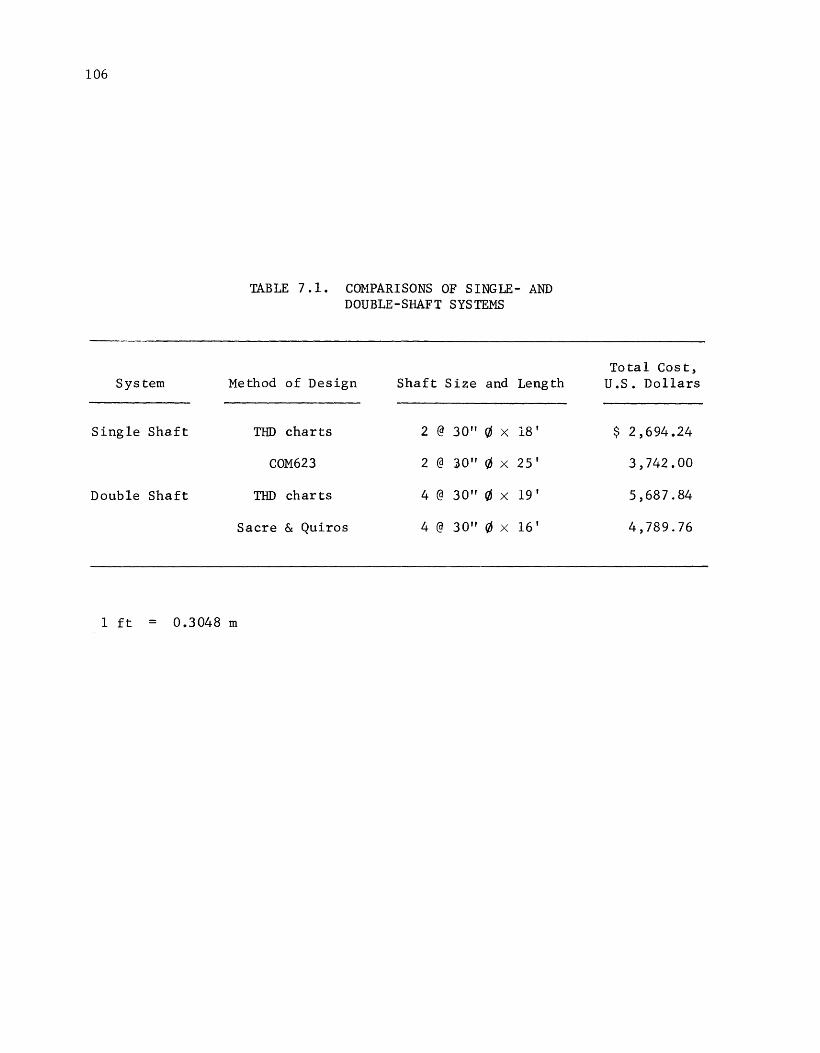
106
System
Single Shaft
Double Shaft
TABLE 7 .1. COHPARISONS OF SINGLE- AND DOUBLE-SHAFT SYSTEMS
Method of Design Shaft Size and Length
TIID charts 2 @ 30" 0 X 18 I
COM623 2 @ ]0" 0 X 25 1
TIID charts 4 @ 30" 0 X 19 I
Sacre & Quiros 4 @ 30" 0 X 16 1
1 ft 0.3048 m
Total Cost, U.S. Dollars
$ 2,694.24
3,742.00
5,687.84
4,789.76
107
Table 7.1 indicates that the cost of the single-shaft system is around
one-half the cost of the double-shaft system. If the desired des~gn solution
is to be based upon such a simplified cost comparison the single-shaft system
would be chosen.
ADDITIONAL FACTORS AFFECTING SELECTION OF FOUNDATION TYPE
In many cases, the decision on foundation type to be used can be based
largely on economic consideration. However, the possibility exists that
other conditions may influence or even dominate this selection. In every
instance the economic analysis must, therefore, be viewed in light of addi
tional variables that are not directly convertible to dollar quantities.

!!!!!!!!!!!!!!!!!!!"#$%!&'()!*)&+',)%!'-!$-.)-.$/-'++0!1+'-2!&'()!$-!.#)!/*$($-'+3!
44!5"6!7$1*'*0!8$($.$9'.$/-!")':!

CHAPTER 8. CONCLUSIONS
DESIGN CONCEPTS
1WO-SHAFT SYSTEM
The traditional form of foundation for the overhead sign structure has
been a double-shaft system. The loadings, shear, moment, and axial thrust
have been resisted largely by the axial resistances of the soil-shaft system
in either compression or tension. This system tends to be inefficient in
comparison to the single-shaft system for most uses and its application should
be restricted to special cases.
SINGLE-SHAFT SYSTEM
The use of single shafts to resist shear, moment, and axial thrust has
been suggested. The proper design of such a system leads to the most effi
cient use of the system materials; the large axial chruscs of the double
shaft system are greatly reduced and at the same time the shaft's capacity in
bending is much more fully utilized.
DESIGN PROCEDURES
USE OF CHARTS IN DESIGN
Aids have been developed at SDHPT for use in the design of both single
and double-shaft systems. These charts were based upon several simplifying
assumptions and failure criteria. The designer should be aware of these
assumptions and limits in order to avoid an incorrect application of the
chart.
109

110
USE OF COMPUTER PROGRAM IN DESIGN (COM623)
The use of a computer program for purposes of design has been presented.
This approach allows a maximum amount of variability in the modelling of the
system and provides an output of the most probable final configuration of the
designed system. Input of data is a simple process and computation times are
relatively short.
FACTORS OF SAFETY AND COST COMPARISONS
FACTORS OF SAFETY
Factors of safety have been formulated and used in the generation of the
SDHPT charts. However, as mentioned previously, the use of a chart for pur
poses of design can lead to uncertainty in the actual factor of safety of the
final design. The computer program presented has no factor of safety. It can
be used for either working stress or load-factor design by the appropriate
manipulation of input or output quantities.
COST COMPARISON
A simplified cost comparison has been made and presented for a typical
design problem. The single-shaft system was comparatively cheaper than the
double-shaft system. Variables exist that can complicate and influence the
design in such a manner that cost figures alone cannot be the sole criteria
for system selection.
SAN ANTONIO FIELD TEST
TEST RESULTS
Results of a test run in San Antonio indicate that current theories of
soil-shaft behavior under loading are correct. The predicted behaviors were
conservative in comparison to the observed behaviors, indicating that design
procedures based upon the theories involved will yield a safe solution.
111
FURTHER RESEARCH
Testing of uninstrumented shafts can be relatively inexpensive, and an
attempt should be made to perform such tests when an opportunity arises.
Testing of instrumented shafts will be relatively expensive but the construc
tion and testing of instrumented shafts will allow further improvements to be
made in the design methods.

!!!!!!!!!!!!!!!!!!!"#$%!&'()!*)&+',)%!'-!$-.)-.$/-'++0!1+'-2!&'()!$-!.#)!/*$($-'+3!
44!5"6!7$1*'*0!8$($.$9'.$/-!")':!

REFERENCES
1. Aurora, Ravi P., and Lymon C. Reese, "Behavior of Axially Loaded Drilled Shafts in Clay-Shales," Center for Highway Research, Research Report No. 176-4, The University of Texas at Austin, March 1976.
2. Coyle, Harry M., Manaf M. Hamoudi, and Richard E. Bartoskewitz, Correlation of The Texas Highway Department Cone Penetrometer Test with Unconsolidated-Undrained Shear Strength of Cohesive Soils, Texas Transportation Institute Research Report TTI-2-5-74-10-1, August 1974.
3. Focht, John A., and Kenneth J. Koch, "Rational Analysis of the Lateral Performance of Offshore Pile Groups," Proceedings, Fifth Annual Offshore Technology Conference, Paper No. OTC 1896, Dallas, Texas, 1973, pp
4. Matlock, Hudson, "Correlations for Design of Laterally Loaded Piles in Soft Clay," Proceedings, Second Annual Offshore Technology Conference, Paper No. OTC 1204, Houston, Texas, 1970, pp 577-588.
5. Mayer, Barry J., "Analysis of Single Piles Under Lateral Loading," unpublished M.S. Thesis, The University of Texas at Austin, December 1979.
6. O'Neill, Michael W., and Lymon C. Reese, "Criteria for the Design of Axially Loaded Drilled Shafts," Center for Highway Research, Research Report No. 89-11F, The University of Texas at Austin, August 1971.
7. Peck, Ralph B., Walter E. Hanson, and Thomas H. Thornburn, Foundation Engineering, Second Edition, John Wiley and Sons, Inc., New York, 1974.
8. Poulos, Harry G., "Analysis of the Settlement of Pile Groups," Geotechnique, Vol XVIII, No. 4, December 1968, pp 449-471.
9. Poulos, Harry G., "Behavior of Laterally Loaded Piles: I-Single Piles," Journal of Soil Mechanics and Foundation Division, Vol 97, No. SM5, May 1971, pp 711-7]1.
10. Poulos, Harry G., "Behavior of Laterally Loaded Piles: II-Pile Groups," Journal of Soil Mechanics and Foundation Division, Vol 97, No. SM5, May 1971, pp 733-752.
113
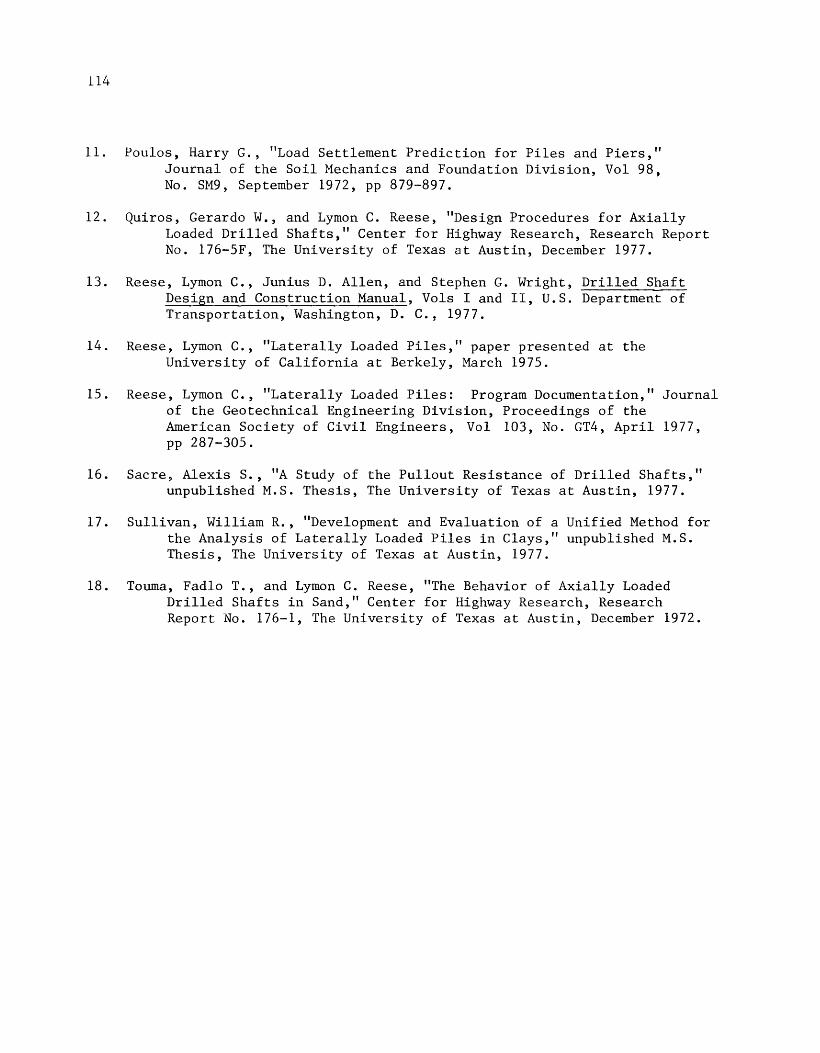
114
11. Poulos, Harry G., "Load Settlement Prediction for Piles and Piers," Journal of the Soil Mechanics and Foundation Division, Vol 98, No. SM9, September 1972, pp 879-897.
12. Quiros, Gerardo W., and Lyman C. Reese, "Design Procedures for Axially Loaded Drilled Shafts," Center for Highway Research, Research Report No. 176-5F, The University of Texas at Austin, December 1977.
13. Reese, Lyman C., Junius D. Allen, and Stephen G. Wright, Drilled Shaft Design and Construction Manual, Vols I and II, U.S. Department of Transportation, Washington, D. C.~ 1977.
14. Reese, Lyman C., "Laterally Loaded Piles," paper presented at the University of California at Berkely, March 1975.
15. Reese, Lyman C., "Laterally Loaded Piles: Program Documentation," Journal of the Geotechnical Engineering Division, Proceedings of the American Society of Civil Engineers, Vol 103, No. GT4, April 1977, pp 287-305.
16. Sacre, Alexis S., "A Study of the Pullout Resistance of Drilled Shafts," unpublished M.S. Thesis, The University of Texas at Austin, 1977.
17. Sullivan, William R., "Development and Evaluation of a Unified Method for the Analysis of Laterally Loaded Piles in Clays," unpublished M.S. Thesis, The University of Texas at Austin, 1977.
18. Touma, Fadlo T., and Lyman C. Reese, "The Behavior of Axially Loaded Drilled Shafts in Sand," Center for Highway Research, Research Report No. 176-1, The University of Texas at Austin, December 1972.
APPENDIX
PROGRAM DOCUMENTATION
COMPUTATION OF EI VALUES FOR CONCRETE COLUMNS
FOR VARYING BENDING MOMENTS

!!!!!!!!!!!!!!!!!!!"#$%!&'()!*)&+',)%!'-!$-.)-.$/-'++0!1+'-2!&'()!$-!.#)!/*$($-'+3!
44!5"6!7$1*'*0!8$($.$9'.$/-!")':!
A .1. PROGRAM IDENTIFICATION
A.l.l. PROGRAM TITLE: Computation of EI values for concrete columns for
varying bending moments.
A . 1 . 2 . PROGRAM CODE NAME : PME IX
A.l.3. WRITER: Gangadharan Menon
A.l.4. ORGANIZATION: Department of Civil Engineering, The University of
Texas at Austin, Austin, Texas 78712.
A.l.S. DATE: March 1977.
A.l.6. SOURCE lANGUAGE: FORTRAN IV.
A.l.7. AVAilABILITY: A program listing is given following the documentation.
A.l.8. ABSTRACT: The program calculates values of EI (effective product of
modulus of elasticity and moment of inertia) of the cross section of
a concrete column for a set of values of bending moments under various
axial loads.
117

118
A.2. ENGINEERING DOCUMENTATION
A.2.1. NARRATIVE DESCRIPTION
A.2.1.1. Statement of the Problem
The flexural behavior of a structural element such as a beam, column,
or a pile subjected to bending is dependent upon its flexural rigidity which
is expressed as the product, EI, of the modulus of elasticity of the material
of which it is made and the moment of inertia of the cross section about the
axis of bending. When the values of E and I remain constant for all ranges of
stresses to which the member is subjected, the flexural rigidity EI also
remains constant. But there are situations where both E and I vary as the
stress conditions change. This variation is most pronounced in reinforced
concrete members. Because of nonlinearity in stress-strain relationships, the
value of E varies; and because the concrete in the tensile zone below the
neutral axis becomes ineffective due to cracking, the value of I is reduced.
Apart from this, when a member is made up of a composite cross section
there is no way to directly calculate the value of E for the member as a
whole. Reinforced concrete itself is a composite material, being a combina
tion of concrete and steel reinforcement having different values of E. Other
examples are concrete encased in a steel tube or a steel section encased in
concrete.
A.2.1.2. Outline of the Solution
The value of EI can, however, be calculated from the moment-curvature
relationship of the elastic curve of a beam subjected to bending.
Figure A.la is a portion of the beam subjected to bending with a
radius of curvature
y
p
p . Triangles and being similar,

Neutral Axis
(a) The elastic curve
NA y
(b) Cross section (c) Strain diagram
Fig A.l. Portion of a beam subjected to bending.
2011
0 0
10'*8 Bars .o
3" a"
a"
Fig A.2. Beam cross section for example problem.
119
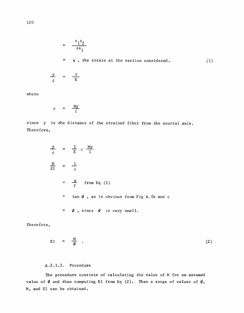
120
s 1 s2 = ss
1
= € the strain at the section considered. '
..L a --p E
where
a = .l!Y.. I
since y is the distance of the strained fiber from the neutral axis.
Therefore,
..L 1 .l!Y.. = X p E I
M 1 = EI p
__§_ from Eq (1) y
tan 0 ' as is obvious from Fig A.lb and c
0 ' sincz 0 is very small.
Therefore,
EI = M 7
A.2.1.3. Procedure
The procedure consists of calculating the value of M for an assumed
value of 0 and then computing EI from Eq (2). Then a range of values of 0,
M, and EI can be obtained.
(1)
(2)

121
A.2.1.4. Example
Figure A.2 shows the cross section of a beam subjected to bending
moment. The axial load is 200 kips (890 kN), 0 = .0001 in.-1
, E = 4000 kip/in.2
(2800 kN/cm2), and E = 30,000 kip/in.
2 (20,700 kN/cm2). Find t~e values of M
s and EI.
As the first step, the position of the neutral axis should be deter
mined by trial, such that the net force on the cross section equals the
applied load of 200 kips (890 kN). Concrete below the neutral axis will be
neglected. A linear stress strain relationship will be assumed here for
simplicity.
Trial 1
c = 9 in. (22. 9 em)
Strains:
At top fiber of concrete: .0001 X 9 = .0009
1st row of bars: .0001 X 6 .0006
2nd row of bars: .0001 X 2 .0002
3rd row of bars: .0001 X 10 .001
4th row of bars: .0001 X 18 .0018
Forces (stress X area):
Concrete: ~.0009 X 40002 X 20 X 9 324 k comp (1442 kN) 2
1st row of bars: (.0006 X 30,000) X 3 X .79 43 k comp (191 kN)
2nd row of bars: ( .0002 X 30,000) X 2 X .79 9 k tension (40 kN)
3rd row of bars: ( .001 X 30,000) X 2 X .79 = 47 k tension (209 kN)
4th row of bars: (.0018 X 30,000) X 3 X .79 128 k tension (570 kN)
Net force = 183 k comp (8144 kN)
N .G.
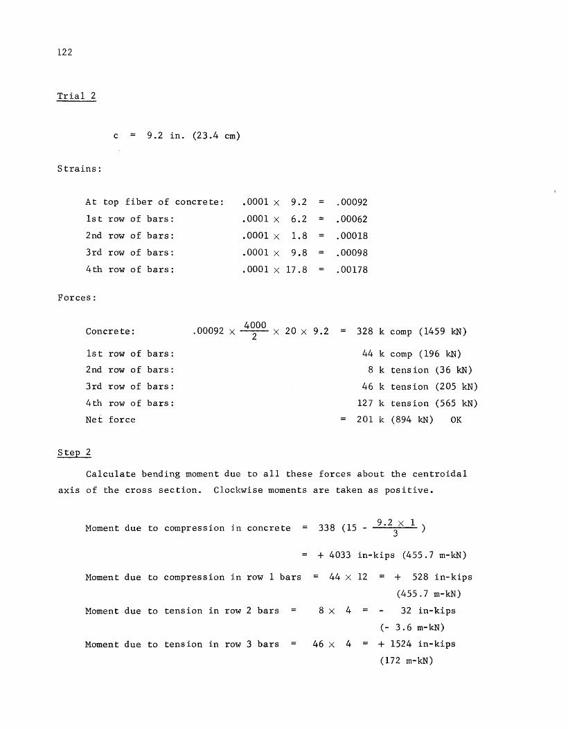
122
Trial 2
c = 9.2 in. (23.4 em)
Strains:
At top fiber of concrete: .0001 X 9.2 .00092
1st row of bars: .0001 X 6.2 = .00062
2nd row of bars: .0001 X 1.8 = .00018
3rd row of bars: .0001 X 9.8 .00098
4th row of bars: .0001 X 17.8 = .00178
Forces:
Concrete: .00092 X 4000
X 20 X 9.2 2 328 k comp ( 1459 kN)
1st row of bars: 44 k comp ( 196 kN)
2nd row of bars: 8 k tens ion (36 kN)
3rd row of bars: 46 k tension (205 kN)
4th row of bars: 127 k tension (565 kN)
Net force 201 k (894 kN) OK
Step 2
Calculate bending moment due to all these forces about the centroidal
axis of the cross section. Clockwise moments are taken as positive.
Moment due to compression in concrete
Moment due to compression in row 1 bars
Moment due to tension in row 2 bars
Moment due to tension in row 3 bars
33 8 ( 15 - 9 . 2 X l ) 3
+ 4033 in-kips (455.7 m-kN)
44 X 12
8 X 4 =
46 X 4
+ 528 in-kips
(455.7 m-kN)
32 in-kips
(- 3.6 m-kN)
+ 1524 in-kips
(172 m-kN)
Moment due to tension in row 4 bars = 127 x 12 + 1524 in-kips
(172 m-kN)
Net Moment M
EI = = 6237 .0001
+ 6237 in-kips
(705 m-kN)
62,370,000 k-in. 2 (179,000,000 N-m2 )
123
The above method, though simple in cases like rectangular cross sections,
becomes tedious when cross sections with varying widths are considered.
Further, since the actual stress-strain relationship of concrete is a non
linear function, for a circular cross section the computation of forces will
involve double integration, one for area and one for the stress. This is not
possible by hand calculations.
A.2.2. APPLICATION TO LOAD-DEFLECTION ANALYSIS OF DRILLED SHAFTS OR PILES
In the analyses of drilled shafts or piles subjected to bending
moments, the flexural rigidity EI is one of the parameters occurring in the
differential equation for the solution of deflections. Typically there will
be large variations of bending moment along the length of the column.
Consequently there will be variations in EI depending on the moment and axial
load if any, and this changed value of EI should be employed in calculations.
A.2.3. PROGRAM CAPABILITIES
Calculation of forces and moments are done in the program by dividing
the cross section into a number of horizontal strips and summing. Figures A.3
and A.4 show the stress-strain curves for concrete and steel, respectively,
used in the program.
The program gives as output a set of curves for M versus EI values
for different axial loads ranging from zero to the axial load capacity for the
column. The number of load cases in one run is limited to 10.
Program options allow treatment of the following types of cross
sections:

124
f~
E -2 .k 0- Ec
~~·
.0038 E
1/2 E c = 5 750 0 { f ~)
f~ is in units of lb/in2
f~ =.85 f~
fc: f ~I r2 {..!.. ) - ( .f_) 2 ] ~ Eo Eo
Fig A.3. Stress-strain curve for concrete used by Program PMEI.
fy
E5 = 29000 ks i
Fig A.4. Stress-strain curve for steel used by Program PMEI.
(1) Square or Rectangular, Reinforced Concrete,
(2) Circular, Reinforced Concrete~
(3) Circular, Reinforced Concrete, with steel tubular around the concrete,
(4) Circular, Reinforced Concrete, with steel tubular tubular core, and
shell
shell
(5) Circular, Reinforced Concrete, without shell but with tubular core.
A.2.4. DATA INPUT
and
The data input form along with the names of variables is shown in
Fig A.5. The variables are defined in Table A.l.
A.2.5. PRINTED OUTPUT
The printed output gives a statement of input values, values of E c
and axial load capacity for no moment, and a table each of values of moment,
EI, 0, maximum strain in the concrete, and depth of neutral axis for each
axial load case. The initial value of moment corresponds to a curvature of -1
.00001 in. . The final value is a step higher than the ultimate failure
conditions of concrete. Values at failure can be read off at a concrete
strain of 0.0030.
A.2.6. OTHER OUTPUT
If the axial load more than the squash load is applied, the program
stops and an error message is printed out.
A.2.7. SAMPLE RUNS
Four example problems were solved. Figures A.6a to A.6d give the
cross sections of each example. For each problem three load cases, 0.0
(0.0 kN), 10.0 (44.48 kN), and 1000 k (4448 kN), were used.
125

(All units in inches and kips) t-'
"" ()'\
1 10 20 30 40 50 60 70 80
A ANA:ME
1 5 10
B I SHAPE NP
1 10
c p (Repeat NP times)
1 10 20 30 40
D FC BARFY TUBEFY ES
1 10 20 30 40 50
E WIDTH OD DT T TT
1 5 10 20
F NBARS NROWS COVER
1 10
G AS (Repeat NROWS times)
1 10
H xs (Repeat NROWS times) Card H required only if ASHAPE is 1, i.e., for rectangular or square cross sections.
Fig A .5. Data input form for computer program PMEI. A description of variables is given in Table A.l.

12 7-
TABLE A.l. DETAILED INPUT GUIDE WITH DEFINITIONS OF VARIABLES (All units in inches and kips)
Card A (8Al0)
Card B (2IS)
Card C (F 10 • 2 )
Card D (4Fl0.2)
Card E (SF10.2)
Card F (2IS,Fl0.2)
Card G (Fl0.2)
A NAME
I SHAPE
NP
p
FC BARFY TUBEFY ES
WIDTH
OD
DT
T
Alphanumeric description to be printed as title
Identification number of the shape of cross section of column/pile
1: Rectangular or square 10: Circular (without shell or core) 20: Circular (with she 11 but without core) 30: Circular (with shell and core or without
shell and with core) Number of load cases (axial)
Axial load. The total number of a)_ial loads per run is limited to 10.
Cylinder strength of concrete Yield strength of reinforcement Yield strength of shell or core Modulus of elasticity of steel
Width of section if rectangular (0.0 if circular) Outer diameter, if circular, or depth of section if rectangular Outer diameter of core (0.0 if ISHAPE is 1 or 10) Thickness of shell
TT Thickness of core
NBARS NROWS
COVER
AS
Number of reinforcing bars Number of rows of reinforcing bars (a number not exceeding 50) Cover of rebar, from center of rebar to outer edge of concrete
Area of reinforcement in a row AS(l) is for the top row AS(2) is for the 2nd row from the top, etc. The total number of values should not exceed 50
Note: In the case of an odd number of bars in a circular cross section the centroidal axis is taken as the diameter passing through one bar. In this case the number of rows will be the same as the number of bars.
Card H (Fl0.2) xs Distance of row from centroidal axis, starting from top row downwards. Positive for rows above the axis and negative for rmV's be low the axis. The total number of values should not exceed SO.
Note: Card H is required only in the case of rectangular or square sections.

128
3 a= 2.37 in-
2. a = 1.5a in2
2 •a = L5a in2
3 *a = 2.37 in2
a)
b)
c)
d)
40 11
Dia.
20"
0 0 0
12"
4+~ 0 0
4" 1-----~. 0 0
-12"
0 0 0
I~ 8 = 0.79 in2 218=1.58
~ 8 = 1.58 .;::;..._ __ ~8= 1.58
2# 8= 1.58
, .. 8 =0.79
No. of Rows=?
No. of Rows =15
Each Row Contains 1=tta Bar
As =0. 79 in2
2#8 =1.58 in2
" = " II c ,,
No. of
" = .. Rows= 7
" = , ,,
= " II = "
Fig A.6. Concrete column cross sections for example problems.

~HAP£ I ~!eT&NGUt A~ wtDT~ 20:0~
No: OF ~~BA~8 t~ ~nws o, QE~&PS a COVft~ CAA~ C!NTER TO CnNCR EDG,) 1:0
LAVE~
1
~
3
ARF£A ~~'37
~~~8
CONCRETE CVLIND!R 8T-ENGT~ ~E84RS VIELO STRFNGT~ SH!LL/TUAE VtELO ST~F.NGTH MODULUS OF ELAST; OF 8TE!L MODULUS OF !LAST. 0' CONCA ~QUASH LOA~ CAPACITY
MOMENT tN I<!PS
ao:2 2~CII;A !~7.13 ~;z:'e 7148;2 q(tl'' l
t0crr;e 1272~~ t441J,7 t~t~,0 t7qt··8 '9641 2 ~11,,1 ~lf1#b 35~7;8 46ttti8 cqqe:l '5316,8 li41~· ~ r;s2e!1 c;~te:7 IJ70t ::,4 5'180f• S8'5•8 sqts,CJ '5'?~9;0 1593l'b ljq]q f.t ljQ]I§lQ ~917!5 -.~Jtt]:. 8
!I t<IP•TN2
IJI.l~,~0Cl;b IHJtb14Ql 1 b (t~tl4A'J'S,8 1UtAbiJb~2,0 44CU3CJ4q 1 0 4J~t,.J?~t0, e 43~1~5,6,2 438b0tao, e 03808261 1 0 D31'5r;q~b 1 2 4!70~t.,e,q 4]bU8220,7 43'!94~A8 1 2 43!13QIHH
1 t
4:5t~b3C7 1 8 40A5~7?Z 1 3 ]lUi51274
1q
30~4R7A8 1 4 2b782CJ4Q,4 2372'58b2,1 213bl9&2,., tfJ458ol.l4 1 7 t78Qbt.1b,Q 16~8R1Ja8 1 Z 15t.&5JQ~1 2 tt.&15&0t3:1 1338~&88,2 t2~4~5A5 1 5 11~01~~2,' tttl97Q5,2 t0~S7J,l.c
4,001<8! b0,001<St •0,001<1!
2QA00 1 001C8t 363b,b21C8t 2481,l41<PS
PHI
;000001
1 000A~5 ,000009
1 Aot0013 ,090011 ,0~0~21 ,~CII~A21J ,01002Q , ~lUJP133 ,000~37 ,0tt004! ,000045
1 0GUHHJQ ,000~53
1 0Qt0ARJ
1 0a0ttl
1 A90143 1 0AA17l 1 0A021l!3 ,090233 1 eiUJ2&3 ,0fl0lCJ! .0A0323 ;000353 ,000183 ,0~0413
1 0A0443 .011J473 ;010503 1 A00533 .0005b3
MAX STR TN/IN
;e~""' ,0CIIOIA4 ~0CIIotg& p0A(II0fl ,eQirH 2
•""'"'1! 1 C!J0PI18 •""'"'21 r fUIQ!Zll •""'P~l7 •"'""'30 •"""'32 ,00(113!
1 00CII~8 •""'&8~1 ,0BA83 •""'t00 ,0At17 ,eA,!0 ,00143 ,00t57
•'"'''0 ,0PJt84 ,0Atct8 ,091~12 ,0~?24 ,0CJt~35 ,eCII~45
1 0Att5b ,00?1»7 ,0A~e0
~~ A X 7 S t~
7,07 7,0" 7,10 1. t 1 7,12 7,11J ., • 15 7,16 7,18 1. 1 q 7,20 7,Z2 7,23 7,25 1,Jb 7,33 &,qq .,,4 ~.4t flt,15 s.q., 5,81 S,bQ '5,&0 5,53 s,az 5,2Q 5' t 8 '5,C'Jq w; • ~H ll,Qg
129

130
c;q43~7 t~PI230et0;5 ;Aett01J.] ;0C'1?~1 l.l,cu~
5942~9 Q~3~t~8,7 1 AIA6i3 •0"'"401 4,8t1 5942;4 qt liHJ2~0 1 4 1 0AA6!] ,01"1'H2 a,,., 59U 1 .·8 8&99592,b ,01.110.8! ,e03~i 4,12 sq'H ~ t 8132485,i 1 0P~It!Tll ,e~,3l ~~~ . ., 594~;·3 7995Ab9
1b ,0CII014l ,011]44 4~62
59)9 7 76A1~9PI 1 f) ,0~~173 •"'"'~IJ4 4~58 ~9!8,'9 7J9S~t8 1 tt .0~0803 ,0ClJ~65 a,ss : 5qJ8t~ 7t2842A 1 '5 ;0AI~Jl •""']76 4~!1 58~4.0 b~lR0~4.& .0008&3 .00388 4,5A

1
~HAPE I REeTANGULAR WIOT~ ~~:~A
NO: nF R!BAR8 10 ~OWS 0, REAlPS 4 COVER t8&~ CENT!~ TO CnNCR EDG~) 1:0
LAV!R t
ORD!NATE" t2:~~
2
3
CONCRETE CVLJNn!R 8TRENGT~ REBARS YIElD STRFNGT~ 5HELL/TU8[ VTELD STR,NGT~ MODULUS n' ELAIT; OF STE~L MODULUS n, ELAST. 0' CONCR ~QIJA8H lOAn t;APACITV
AX!AL LOAD •
MOto1ENT IN t<YP!
t t 3!18 2~Rttc~ 415~14 bc;t!•t 82&C!J
t00t!"'1 t l 71§{·4 t 349~'13
' , t 52~'.'7 t &9~;!7 t 8&8~"3 2040~14 22t2;0 23A3'·'2 36~t{2 4Tu~;q !089' .1 !442{~q 5540''1 '5634!'1 !721:2 ''"'b !·tS 58~4!'7 5958 3 602'7,46 b037!o b04f)'~' 12 '!48,f0 b049f7 60~0:9 f»0'52!0
EI t<lP•JN2
U 37841A2;et ~9176"~2,1 52A217'14.5 50A84t29:u 48ft0Ao~9;u 47&7t2iH.S 47~1Ci2ft0;3 4&,2'12AA 1 1 4&t42849
1s
4582Q8c.;9,2 455b8413 1 A 45,42145,3 45143&&4,2 4ll~bb0fl3,c;
t1'39903At,q at&~97~0,e 35'59?'5~5,4 '1~b2~~2,J 2'7,91242,7 l4tA081Sb.7 211537"9;5 P~A 17~f.tQ: l !821~0:17,~ to~18Q912 1 8 1~?31890,9 t 4f.t18Q'U ,4 1]~48]27,' l2'78f»~,,,,
t2~2'12Cit"•l 11152483,9 1014~537.2
4,00kSt ._ra,run<sr .e,e0t<ST
2Q000,0fikSt 3f>l6.fJ21<8I 2481,tAI<PS
PHI
; rtlfH!IOII 1 ,0~0"'_1!15 ,(.1)~000. .0li110Pit3 ;0eR011 ,~A0~21
1 ~HHH~25
1 fltCit002q r (.'HH~t'133 ,~Hl!OI037
1 Alll00141 ,00(.11~4'5
1Af!Cit009
'""00§1 1 A0t'1083 ,A09lttl ,0JII0t43 , Ol~liH 13 ,0~0203 ,0fl02l:S 1 0GHl2ttl '""'0293 ,000323 •"'"'~!53 ,QJ9J0]8l ,000141] .00044] ; eHIJ04 71
1 C'Jr~UII503 ,aft0'5l3 .0005&3
MAX 8TR TNJIN
;e0,e2 1 001C~t~5
,001'108 , 091t1it t ,091013 ,~ArHb ,00~1Q
1 1itl'liA22 ,000925 ,errHl!28 ,189109:11 ,0SJ~ot]4 ,00(JI37 ,0AQI40 ,00101f.t2 ,00085 ,0Pit02 ,0ftt1' .00t32 :e91,4b ~00159 ,e.,173 1 0At87 ,001~1!11 ,ePI~t• ,011'211 , IU1,240 ,00~50
• '""~· 1 ,00272 .00283
N AXIS !N
16,'55 Q,IS\ s,t;, A, t t '7,91
'·'' 1,6Q 7,&3 7~5Q 1,5b 7,54 1,5! 1,151 1,S1 1,53 7~4q 7,tt f.t,88 &,52 b,f!b &,0& 5,'12 5~79
5·'"' 5,63 5.50 1§,41 113,30 s,20 cs,tt 5,13
131
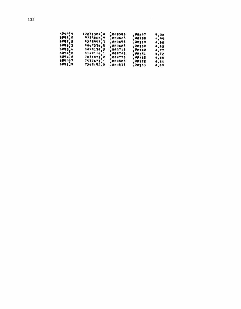
132
b0001Q t0~7t:seo;a ;0005Q] •""'''' 5.~~ '"'~e!e Q1ilSbb
1Q ,eQieft23 .00,~8 4.QI§
6C!f57:2 Q275Q01.1 '"'"'"'&!] ~BA!tQ a.se 60~ttt3 A~b12lb;5 1 RAAb83 ;~0]3A a.e2 60~!;b 8QQ~1~0,2 1 00A713 •'"'4" "·'' 60~4~'8 ~H,Ot16 1 1
1 90R741 .0C!I]51 a.12 60~4;0 7~]1811,~ ,0~077] ;0"']·2 4:•s ftlt;~-,., 1!1;37fl7t,t 1 ftQJAA03 ,011]72 "·'4 60~! !'-Q 7~b5tt:;2.0 .000831 .0A]83 a.ll~
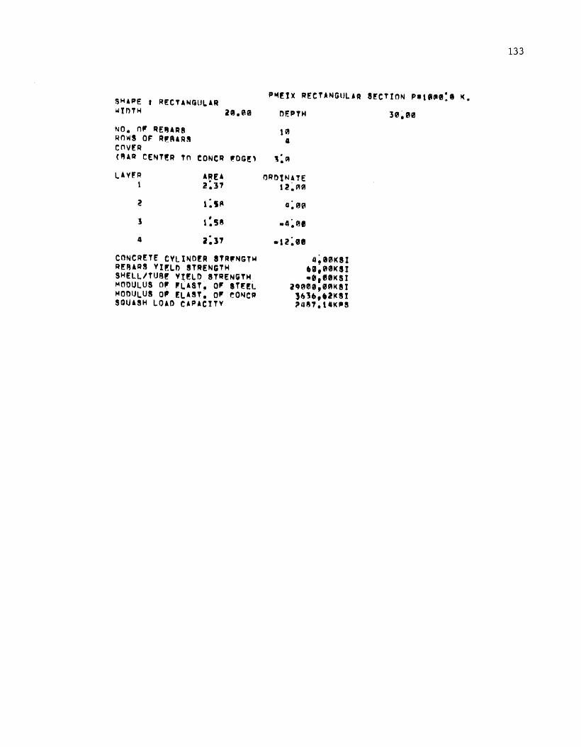
SHAPE I RECTANGULAR ~tnTH 21.09
NO. nF RE~AR8 10 RnWS OF RF.AARS a r:nve:R (~AR CENT!R Tn tONCR ~OG!l 1:A
tlRO!NATE LAVFR AREA 2:3'7 1
2 l: '" 3 1:58
4 z::s'7
CnNCRETE CVLINO!R ITR'-NGTW REAARS VI!LO STRENGTH SHELL/TUB! Vt~LD STRENGTH MODULUS OF PLAST. OF ITE!L MODULUS O' !LAST~ OF eONCR SQUASH LOAD CAPACITV
t2~A~
4~101<81 •ta, GH11< S l •ll! 1 fJII<SI
lCUJ01,0PI1<81 163···21<81 ~48'7.1111<.-S
133

134
A)tlAL LOAD • lA0CtJ.~~ t<IPS
~OM~ NT Er "Hl MAX ST~ N AXIS IN I<IIIIS I<YP~tN2 !NJfN IN
t4J;Q t439411t1~Q ;"-100801 .V10041 4A2;7t 710 ~ 1418!201~,, •"'"'~001§ ,00054 t08,b~
12q4:A t4!1770&t,~ ,'!AQJI0q .A0CII&0 61,18 18bfl.~ t4Js••za8,1tl ,e0eet1 .A01tb7 !t,l~ 243·~· t4J348•4•,• •'"'"'' ~arutyl 42,91 1003.7 !430J5'5815,b .. QJ0AI2l ·"'e''' s,,.,. 31J•6;4 t4l'-'475o;• ;0010125 ~eeCJJet J4,3~ ~'124.0 t422QI.b31,5 .~~0029 .00092 31,8t 4Et''O: 0 t4t'78qt8ct.Q ,00Q9~13 ~P.I0t•• 29,,, 5t84~t' t4"-'lt4]~Q~b ,"-'0~9]1 ,001~~ !8,4'7 5et'7,5 13101 34WJ,4 ,AOtt'tP.IQ1 ,A0t12 l1,2l bA0B.~ t33l!t'7qo.s .0010115 .A0tt8 z•,tb b'Joo;a 1204684tQ~~ ~AA004q ·"0t~4 25,24 bb56,0 12558308~,6 .~A&IJI5] ,PI0t30. 24,44 8J4A,o 1004~61.144,4 ~0A00A3 ,00!71 l0,.Q 9414,2 813tl~JQ,q ,A~Oitt] •"'02\2 te,e"'
UH2!, t 7teJ2542~8 ;:a"'"'14] .00~1156 tT,se 1043t,4 b~~q&82115,, ·'"'''It?] ,10]g4 17,57 tl62tJ,'7 52343l4tJ,t ~9002"-'3 ,001-;S 11,50 10bl6.11J 4565007~.~ .90021] .004Ab 17. '"''

S~APE I CtRCULAR ntAMETF.R S.,.~LL THir.K,!fS COR! 'rUBE 0.0: Cf1R! TlJRE T~tCI<IIJESS
30.00 •Cit.,QI •0.GII0 •OJ.~~
NO. OF R!SA-1 tz ROWI OF RF.AARS 1 COV!R (RlR C~~T~R Tn CO~CR ,OGE' 1.QI
LAYE'R A~El t :7CJ
2 1:58
1 1: se
a 1: ~e r; t:se •• :GIJ0
6 t:ss ., :7Q
CONCRf'TE rYt.lNDF.R STRP:NGTI-4 RfRARS YI~Ln STRENGTH S~F.LI,./TIIB'- VI~Ln STR'-NGTH MODULUS 0, £LAST. O" ~T~EL ~4 n f) lJ L II S 11 F P' L AS T • 0 tr r. 0 11.1 C R ~~IUS~ 1.0Ar> CA"•CYTY
a~98KII ft0."0t<Sl •11.901<51
2 Q ~H~ ~ • 0 01( 81 1&~6,~21<Sl ~QJQ.&fll<ltS
135
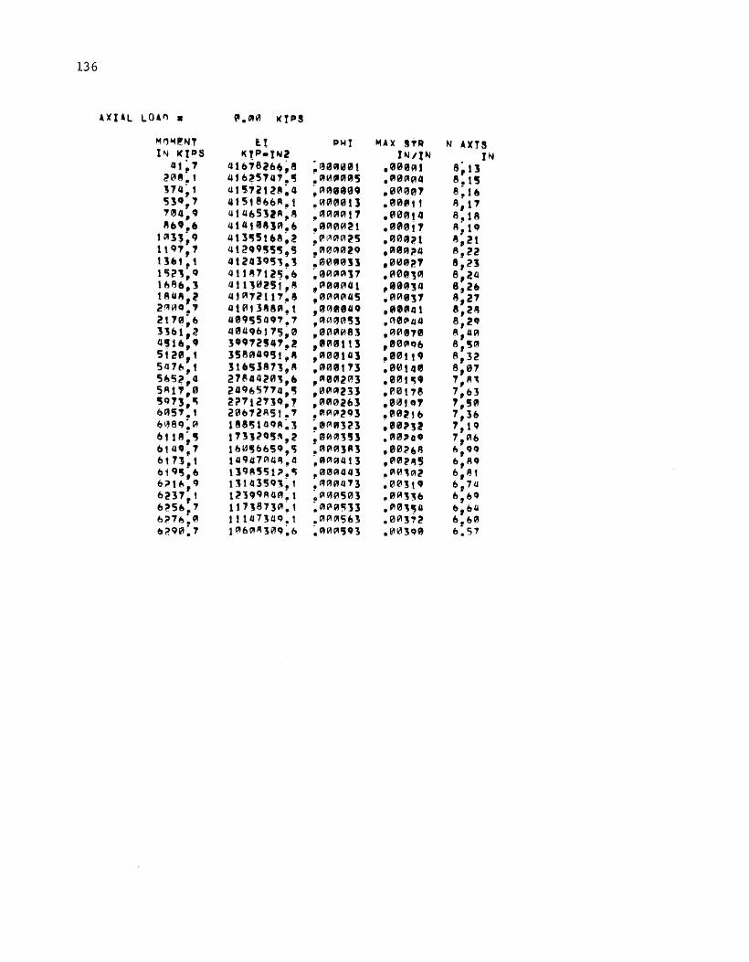
136
AXIAL LOAn • ~.otVI I< tillS
M!1~'-NT Et Pl-4! 111AX STR N AXTS I~ !<IDS KtP•tNl I Nit~ 1"4
Qt~1 4U~18261)~8 ;~ae~t0~H .000~1 8~1] ~~8.t 4!6~5741.~ ·"'~"'~95 ,PI9~04 e.t! 374~1 at51it28~4 ~~(;9f11199 .0~007 e;t6 53CJ,1 4t5t!boAat .00QHH 3 • G1H'HIJ11 A1 t1 104,~ "l465:JIA~A ·"'""'017 • 00CH 4 8,18 A&fl,6 4t4ti8JA.6 ~0010Vt~t .009!1 8.1Q
1013l,9 4t3~5u~a~! ~(ll~"'"'25 ,00"21 e;2t 1\Q1,1 4t2~9~-s~,s • QH~Ol0iC) ,C39A;t4 s,~~ tlftt,t 4l24]Q5~.l :00flta11 ,000~7 8,21 1'5?'J,C) 411~1tZ,~6 ~~~""'~11 ,lii0~]CIJ e,2a 1b~6,l 4tl~W1l51,8 ""'"~"'41 ,aa934 8,26 l8lH.,2 "''"''~111,8 '""'"'"'45 .008]'1 8,21 2~"'C)·' 4t0tl8@U'I.t ,~~184C) ,lliP!Qt 8,28 2t70;o 40955QC)1:1 ,A~HH~IS3 .cHIC'ta4 a,l~ 33at,f! 404C)6t'1,~0 •01iHI9083 ,"101!78 s,a'-1 4'H~,• 3CJ~72,47,2 1 1HHU t 3 ,e0ot~6 a,~~ 5t20,t 358A4CJ5t,8 ,"-100143 .e0tt' 8,32 547b,! 3l.'J387],A ,00QJt13 ~00tQ0 8,01 5b5~,4 27lHt42"'J,ft ,CII8012"'3 .00t~· .,,~~
5At.,,0 24Q~S1'74 1 1$ 1 0fM123J .eet,e 1,&3 IJQ13," 2tt'?tc.,lo,., ,0Qt026l .00tct7 1,!50 octs'·' 20~7lA51.1 • ''"""'2C)3 ,09~16 1,3& 6~eq:c;, 18815tGCJA:l :e~"'fl323 ,e0~1Z 1,tQ 6ttpt~~ t13J?Q5~,2 ~0~(!13!3 .Q~e,.a• 7,06 bt4CJ,1 16~~b65CJ,s; .0ll'A]R] ,00?68 b,Qq bt11,t t4947AI.i~.a ~API'l4t3 ,00pq' b
1AQ
b;CJ~,o t]9A.5'it;t~il) ,00~443 .~~,,l 6,8t 6;»tb,9 tJ14315C)'J:1 .~~~IIJLI13 .00JtQ 6,7t~ 623'7,1 1?3QQA4A:t :"'~"503 ,0"'1~6 o,&q 6~56,7 lt1J87]A:1 :01P~~]] .~1211~" b,&a 6~7e." ltl4734Q~t .OtPIOIS63 .0A31~ 6,60 02911':'7 1~601AJ0CJ:o :"~"'~'3 -~~]Q9 6.51
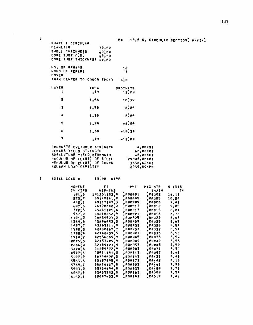
1 SHAPE I Cl~CLILAR OIA~ETER ]0:~0 S~!Ll THTCKN~SS ~~;~9 CORE TUR, n:o: !0rA~ cn~E TUA, T~tC~N,S~ .~.0~
Nn: n~ R,8l~S !2 ROWS OF RERARS 1 rnVEP tRAR CE~T!R TO CO~CR E~G~) 3:0
LAVER t
AREA ,1q
ORt"'tNATF. 12:00
2 1.~8
3 t.!;A
IJ t,58
c; t.58
~ t.'58
7 ·'q ~ONCRETE CVLIN~EP STRENGT~ REAARS VTELD STRFNGTH SH£LLITUA! VtELQ STRFNGT~ MOfHJL US OF EL A 8 T; OF S TE-,:L MtlDlllUI OF ELAST. OF CONCR SQUA8H LnAn CA~AClTV
AXIAL LOAD a 10:~0 I< I"~
MOMENT Ft TN I<TP8 I(!P•tN~ l~t:3 lCII1~5t123 1 1.1 27'5;' 1515'"~ql!lt,0 442~1 UCH11lt1,,3 ofll,~5 llb72--~IJ~,"' 77, .. ~ ll54411P'5 1 f.t q:47;t.i ll4&1A~~2,CJ
t 101 e IHIA3Q593, 2 t2b4'b 43~06011;3,2 t4i»7:7 4Jilf.a'J2t 1, q t'5~0t3 42Q608&1,7 t7152,4 42'1424]9,~ 1 9 t a ~·2 tll'5368,q,q l015}3 ll2,5'\4~'J,9
fll216'0 42t8912t,4 ]l.l~ll:b 41259812,q 4577l8 40~! t UH 1 2 'Slct7;2 36~41l0le,z 55&3 .• 1 3215'1895,4 t;7,.~., 28"74147,8 'S"'CII3 1 0 25131Jbctll,~ &~15,,8 23CII3131l2 1 8 b1~2•·t 209CJ7~2l.9
l.laCIIPUCSt o0,1~~<sr
-~.~01<5! 2Q~00.8RIC~t 3tl»l&,~21<SY 2CJ3q.eqKPS
P~I MAX ~TR hJIIhl
;00000\ ~0~(1102 •"00"'(1115 ,0PIQ!It15
•"'"""eq ,0ftp~6
1 A~00!"S ,0(11~12
,010"'1' ~~"'VIt5 1 QtfHI! Ql Z t ,0"'"''8 •""'"'"'2'5 ,0tl!t'l22 1 Pt9eV12~ ,00C1125 .PI&IIACII'Jl ,0(lt"28 ;(,lJCJI~tl!J7 ,~QI~]2
.~"'"'~4l ,0P~p35 ,00f1Gll45 ,0fltl!'J8
10CII00149 1 eC~tt'11.12
1 0CII005] .0flfl4! ,C'tfl0083 ~0CII011 ,~QI~tt] .~C'tAC'i7
10QICHtJ] ~f~P~!2l
,OJfl~\71 '0"''·"2 1 Ct\CIIA203 .~~'~t•t ,00023'3 ~"'~;a0 ,~0PI2f.t3 •""'2"'0 ·"'"'~~ctl .00!~19
137
N A )CIS !~
1&.t3 10 1 2A q~ut q.~s
B,t'1 ~.1b 8.&8 &.b~ P.,l§~
~.'57 e.-;~ ~.'54
R.'5~ 8,52 R.'54 a.&1 A,l.l] ~.te ..,,qJ 7.73 '·~q '7,4&&
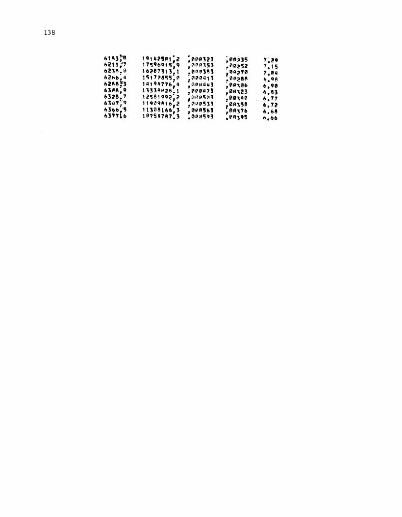
138
t,t"]~0 tfJ14(UJC'It;2 ;l'Pfi32J ~i""'l5 '~l~ '· Etitt;:"f 17t;.e,q1~,, ,~l'l~l53 .~A~I)2 7,t5 &23~:0 to287ltl.t .0C,0JAl ~~91~10 7,14 621\b:4 11517~811§5;0 :"'~~4tJ • 0P!;H'~ &.qB &l~e~l tUt~IJ176 1 4 ;091"''-'43 ~0~,~~ ~.,e 63.,.8:Q 1333A0~8.1 ,0P0473 ,0ft1t]23 6,83 b328:7 12'58199~:2 '0"'~t;03 .00~40 &.77 &Ja .,:·q 11CJ~I.l~,6;2 .A~~I§33 ;0A31J8 1»~12 #} 3~6 ['5 11~08166,3 ~0 .. t'1~6! ,~A~7b 6,68 6377., tk175Ll787.3 .0~~1§Q] .0~]·5 b,bb

81-tAPE I r.I~CIILAR
DIAMETER ,0;~~ SH!LL TMtC~N'S~ .0,~0 CO~E TUB~ n:~~ ,~,se CORF. TUB'- T~tC~NESS .~.~~
NO: OF RP'BlRS ROWS OF R!FURS Cr)VF.:R t~AR C~NTE~ TO CnNCR EnG£)
t2 1
LAVE~ , AREA .79
n~OtNATE
t2:"'0
2 t.~s
'3 t.~e
4 t.se
~ t.~8 , 1.58
7 ."1Q
CONCRETE CVLTNO£~ ~TRENGTM REAARS YtELO STRENGTI-I SH!LLITU~~ VtELD STRFNGT~ MOOIJUJS I"IF ELAST: OF STEEL MOoULUS OF !LA8T: OF CnNeR SQUASH l~AD c•PAClTY
A)(IAL LOAD • 100~:00 I<TP~
MOM! NT P'I TN KIPS ttiJ'eJNlt
134:7 1347229t&;t 6;3:'5 t34&9tA07 1 2 t2l1~0 13U&18911 1 1 t 748,'6 tl450a-;,o,2 2283~~q 134348/H ~, 5 28t1:2 l3l!150l125,4 331.1'' 7 t'J3~0~1~7,& 18&9!'7 13]G3~7&CJ 1 4 431.12:3 t3t-seJ~~7,~' 47~1tA l2915Qt210:3 'i13b:q 125,CHI~IJI.I 1 8 ~475:•1 t2t~>o~q52 1 a 5718,1 117()19118:5 &eb3.15 11440~710,1.1
1tt68~3 '12]88&At 1 '5 aTCJb.7 778"bCJ12.o ~&55:~ t.751776t;3
11:811 t'~J 5CJ&~llltt,t 1 ~·~T 1'5 52&CJ12~t,3 , utA4t ;z oo-;285~7,5 l(ll8,8.'5 Ut,63tfJ9.q
u( 1~
"·001<8! 1)0,A01<St •0.0AkST
2Q~00,PI0KS! 3~3.,62~ST 20:S9.891<PS
PHI MAX ~TR JN/IN
;~"'"'~"'' :1'10~140 t"'PI"'0~5 ~00!0!4b ,P~C'I~PI~Q .0~~52 ,0~~~1'3 ~r1C'!PI5q •"'"'"'017 ,0C'!Pib5 .fl~0021 ,00~1t ;AO!"'A25 •0"'"'"7 , k.H?IPI~29 ,1110~4 ,~091033 ,l'lrA(A-.0 .~C't010137 ,0~~Qb ~0~Pt041 ,0~'"'2 '""'~fl4~ ,0"'·"'8 .~~l'IOII.IQ ,0~1t4 ;e~PIA~:! ,e,.,tCJ ,01910~83 ,!1~~100
.0"'0111 .01tt• ;~""~14] :00~]8
1 llUU!Jt 7 3 ~0A?79 ,AA0~03 ~00~23 •"'"23! •""'J'& .0C'tA?&! .A04(11CJ
13-9
N A'lttS TN
l.t02.'51 9?.~8 se.21 4f0i.03 3e,otA 33.80 3"·'2 2~.84 21~24 2'5,95 24.~7 23.qb 2l.t7 22·"" 1C,.23 17.'5' t~.&7 1&.1& 115.CJ2 115.12 tr;.r;~,

140
S~A~E I CYReUlA• DIAMETER !H!LL T~IC:KN!SS Cl'lRE TUB!: o:l)~ COR! TURE T~ICKNESS
'-'0,'-'~ .c;A
-~·""' ·"'·jill~
j:J.
NO. 0~ REAA-8 1~ Rnws OF RFBARS 15 cnv!R (RlR CENT~R T" CONCP ,OG£\ ~:~
LAVF~ AREA 1 :7Q
2 :7Q
:s :.,~
" :.,~
'5 :7~
~ :7Q
1 :.,q 8 :.,Q
q :7Q
~~ :7Q .. #,.11
l t :7q
12 :7Q
!3 :79
14 :'7Q
tS :7Q
rnNCR~TE CVLtNOER STRPNGTH OF.BARS VI!LO STPENGTH SHFL~ITUR! Vt!L~ ~TRENGTH ~OOULUS 0, !LAST. OF ITP!L ~nr)IJLLIS OF £LAST. OF eONCR S~UASH LOAD CAPACtTV
4p0!KSI ~0,.9(1)~81
1&.G91KSI 2qA~A, 001<lU 'e,~tt,&2K8I ~CJ&&.Bli<PS
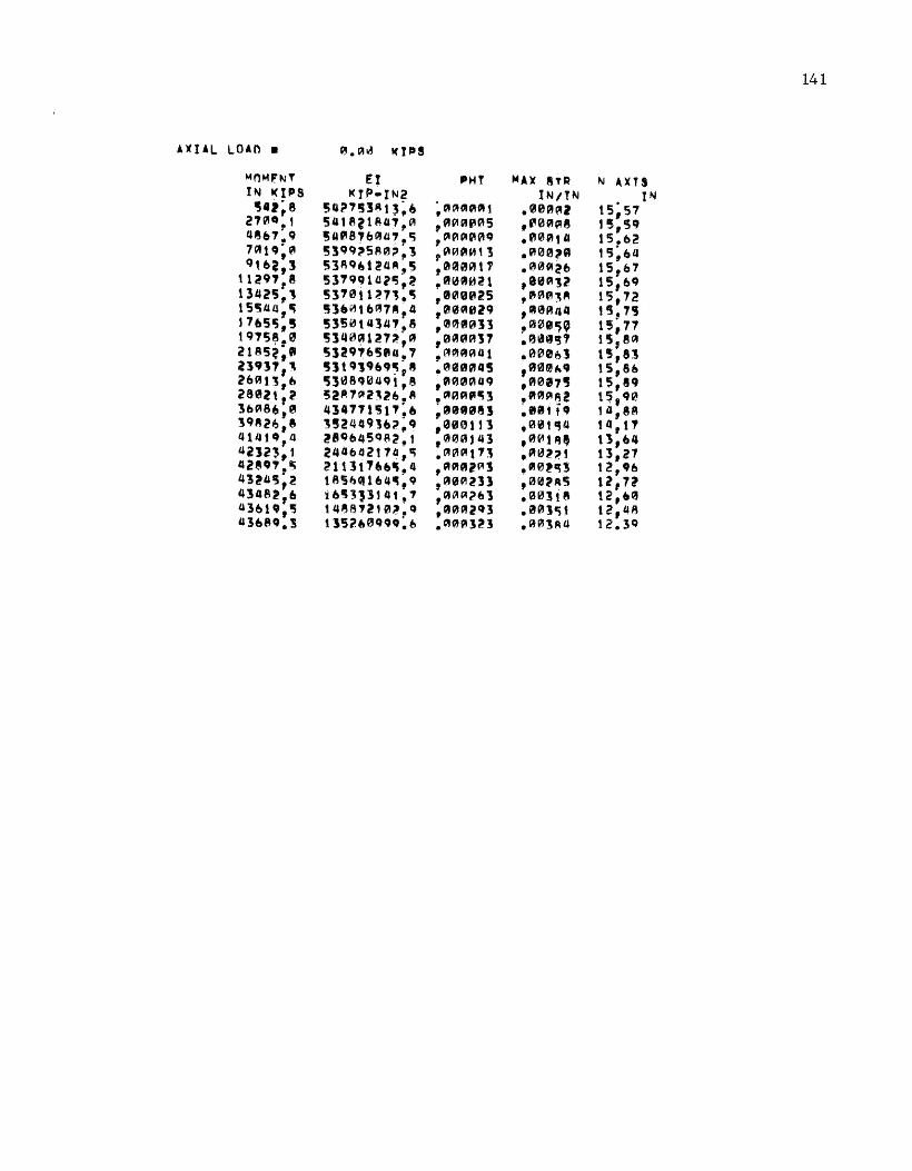
141
A)(JAL LOAn • 0.01~ t<t"S
MnMF~T Et 'Ht ~AX 8T~ N 4)(TS IN t<IPS t<tP•IN2 INJJN IN ~·1;8 ~Q~1~l"'t~~& ~f/t~C'I~H~t .(IJ0PJ~2 ts;s1
2'70",, 541AlHU&1,A ,0~0005 ,fl00018 25,~9 aeo7,.9 !Ulll87oOJa?.t; ,C4PI01009 • ''"~0tll t5.o2 7PJt9~Q! 5]QCJ~SA~~:l ,~"'~"''5 .000~1 ts;oa 9u,, 3 53A9ttll4~:~ ,~0"~'' •00CII~b 15,&7
tt297:e 5379~to;u;;~ ,Af6QI0~1 ~90CII'32 tS,o9 1342'5,1 5370tl~'71.1§ ,eftH1025 '"0C'IJ~ 15,72 15'5tli4,r; !Sl&"'to"7e,4 ,000029 ,~eAa4 t5,7'J 17ft51),! 5]50t43U1,.8 1 QHHt013 ,0011$~ 15,77 1q1se.0 5140~1~'7~,~ ,0~~017 • ~HhJ'!' ts.,ee~~ 21A5~;~ 5]!q1Et504.7 ,t:-.9HHH11 .0006] 15;83 il'J31,1 5319]969~~8 .0a~1QUI5 ,000~· 15,8& 26~t3,b '53"'8<H~a9 t, e ,000049 ,A017! 15,89 28QIZt,2 ~2~70!2J26.A ,CII0Afllil ,CitC'JA~! t$,90 3b086,ftll 41411151"'~6 ,101081 .111f"t 1a,es 39826,8 '3!24491o;»,9 ,caetH 11 ,00!~4 t4,t'P 414t~,a ;?8Qb45Q82,t ,00~1"3 •'H't~· t1,64 ~23Z~,1 2t.a4ba2t1a,~ .AVlPit11 ,Ae~~' tl,27 42eo,,~~~; i?11lt'H•&I5.4 •"'"'R2C'I3 ·"0~r;3 t2,0b 43~~5,2 t 8$6111 bl,plj ~ q ,90~231 ~00,A5 tl,1l 4348~,& jb~'Jl1!4t~' ,A~~261 .00lt8 t2,&~ l.ll&t•,-s 14~B,Z10~.q ·"'"'"'~93 .~0]t;i 12,48 43689.3 tJ'52,.etqqo:6 .A0Cll3~3 .~0]R4 12.3Q

142
S~APE I CtRr.UlAit OfAMETE~ 4A,0~ SH!LL THICKNESS ~~~ co~~ TUR! ~.o~ -~.~~ COR~ TU~E THleKN!~I •A.~~
Nn, 0' RE~ARS !~ ~nws OF A!8ARS 1~ COVER (AAA C!NTPR TO eoNCA ~OGEl 1.0
L•vrR AR!A ! :7Q
2 :7Q
J :.,. 4 :,. ; :.,. 0 :'7Q
1 :.,q 8 :'~ Q :., ..
t0 :.,q
' t :.,q
1 2 :.,q 1 3 :7Q
14 :7~
tS :.,. CONC~ETE CYLtNDF~ STR~NGTH RFAARS Yl!Ln 8T~ENGT~ S~ELL/TUA! Vl~Ln ST~E~GT~ MOOIJLIIS 0, '-LAST, O' 8T!f:l Mfli1ULliS OF FLAST, O' rONCR SfliJASH LOAD CAPAC!TV
4 1 1l1QII<SI b0,0~1<8I 3ft,CJ8~SI
ZQ00~~1lJ~I<SI ~bJb~b21<8l b9bo~"'ti<PS
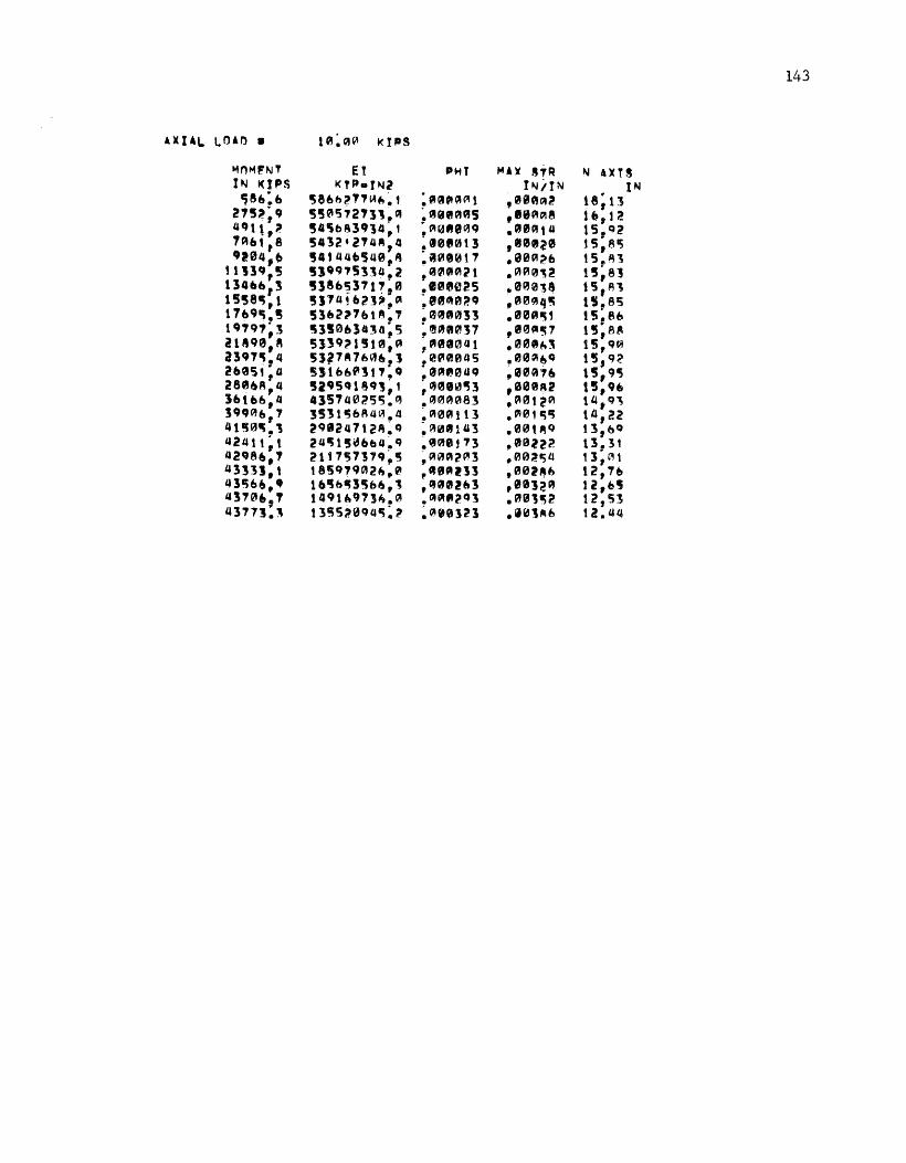
143
A)(IAL LOAn • ta:"~ ~IIIIS
MnM,NT E! PHT MAX 8TR ~ 4XTS IN I(JPS ~TP•IN2 IN/IN IN
c;e&:& '58bb~''"'"~' ~fiQ)~~~~ ,09AA~ te;tJ 215~~9 55Qt'5727l1,~ ~ CUU!A05 ,IIA018 u~,12 4~1\,~ !4'5b83914.1 ;Ara~teOJq • CUJ0 t a t5,Q2 1A&t,8 54l2•274A~4 .1011013 ,101~0 15,815 9!04 ~ IJ4t44bl$4"'" :~010t7 ,90C11;.>& t5.~l
!t13fl:5 SJ~975~34,2 ,0001(11?1 ·"'"'0~~ 15~8! 134ofl1 3 ~38&~371~,0 .10(90~5 .. 000'J8 t5,A3 1558~,1 5]14!b~J;t.C'I ·:e8~0;?9 ,009tq~ ts,es 11&9-;.1§ 5lb2~76tA:'1 ~00fJ03l .00A~1 t!ii 1 8b 19797~] ~3!0&3434;5 :~"'1017 ,GIJ0~~7 15 1 8A at~qe,~ 5Jl9t:Jl1Jta,A ~CIIIQJ041 .008~l 15,q0 2397,,4 5JJ7A7M·~~] 1 ei2IOJ04S ·"""'&q t5,q2 2ft0S1 1 1.l 5Jtbbfl]t,.Q ,0Cltf.t01.lq ~ IUJG1116 15,915 280~A,4 5211f5~te91~t ,C,010'S3 ~00QJ"2 t~,CJ& 3&to&,~:~ 43!7402515.'-' .~"-101083 • CH'Jt ~01 t4,q~ ]9CHlt.
1 7 35ltt;bA4~.4 ~0100tt3 .Ct01-;~ t4,22
41~9~.1 29ll247t2A~q : ~frUH 4 3 .00t~Q t3,&Q 424tt~t 21.11§t5~bfl4~q .eot0t73 .0Bl2~ 13.31 42Q8fJ,7 ;?lt7!;7]7q~~ ,~0~2PI3 ~00~154 t 1; en 4333J,t t85Q7902bp0 .. cuutzJJ ,00!~b t2,16 43c;b~,· te.i!b~3~b~,, .~002ft3 ,1190]~~ ti,b~ 43'10b,1 t4Ql,.CJ'73~.0 .ot~ft2ql .AS1t;2 12,53 43771.1 t3155~0qq-;:~ ~~101~3 .1101~b ti.IJ4

144
SHAPE I CTRCULAR OTAM~TE~ a~.~~ SH!LL T~IeK~ESS .~~ CnR! TURE o:~~ •0o00 COR! TU8E THtC~NESS -~.~~
Nn~ OF RERARI 1~ Rn~s OF ~~AA~S t~ r:nve:R fBAq CENT~R T~ CONCA ,OGE' 1.~
LAY~R AREA t :7Q
2 :7• 3 :7' Q :7q 5 :.,. 6 :.,. 1 :.,. 8 :1C'i Q :7•
t£'1 :,q t 1 :.,. 12 :.,. ~~ :7'1
\4 :,., tiS :1•
CnNCRfT! CVLINDfR 8TR,NGTH R~B.RS VI~LO ST•E~GTH S~!LL/TUB~ VI!~n ST·E~;TH lo400ULllS OF ~LAST. OF STE~l M~0ULU8 0~ !LAST. O' CONCR Sl'liJASiol LOAD CAPACITY
"RO!~AT! u.:ot
t~:.,
t4:!•
~~:~&
4,981($1 &0,001<81 Jft,IIICII
l~090p001<11 1&1&,o21<8I ,cu,. • 9l1Ut5
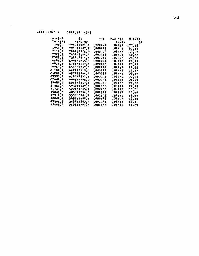
145
4'1CtlL LOAn • 1000.1~ l(tPS
MnM~NT [t PHt ~AX 8T- N AXt! I~ ~ttts l<f,•IN2 INitN IN '"'t;" '1QtCJGt~'-'1:7 ;9Jt;'l~~~t ,cHJA~8 177;fJ2
3~5Q,l .,,1847,87~2 •"810"$ .00~2& st,&t 7,t6,e 7Q01,07?6,0 ,001~09 ~fi00J3 31,&1 Qqll,l ?&l2Gll«~~.o 1 QIPI0~tJ ,llatllttl 'J2,fl7
t2'3Q2,t 72~94?!71,8 ,0AfU117 ,eae~qe za,ee t46Q!,8 6998~2"'3~.8 ,9Af!02l ,0"'0135 ~,,.,,
16916,1 6766~3687,& ,10~1JZIJ ,e0tt~?. !!,!2 lQQie,~ ' &5'1561~3.,,1 ·"'0"'029 ,llfl~lf 2",12 2118,~4 64210211~,1 ;a0QJC!I13 ,0007'3 23.)7 23282,7 fo12'2&19e4,o ,300037 ,10Cifllc;a 22;&"' 25354,7 &tfUU1'13ta1,& ,4190Clt041 .eeeaq 22,14 2740'·' 60CJ 11!,400~. 0 .~00045 .f!l0fQ5 ~!:;: 294SIJ;q 6010~931?~6 ~00A0tJQ ~00t9ti! 314&8," S9J7J!,4?,1 1 0080Sl ,eeu,., 2e,•! 11'?Jta
1115 '50288!245 •• ,BClt"'08] ,10!~8 1,,5!
4584J,e 40!&1f7!J4~~ ,ll~tll .10!015 1&.&4 4?Qt2,0 :J]501l8'hH: 4 .000143 ,0011Jl !8~04 4884~.~ !8236160t;;b ;eelt'13 ,10~07 17,·~ 4Q~•t,l 2426~·2~:!," ,t'-'012~] ,ee1a3 t"f,IU 49468.• 2t23tl107.~ ... ~~211 .IB!~t t7.zq

146
~~APf 1 CHH~ULAR DIAMETER SHELL THIC:I<N~SS cnRf: TURE o:o~ CnRE TUBE T~tr.K~E8S
48.00 .11§12J
10.90 .~8
NO. OF R!AARS 14 ~n~S OF RERARS ' cnvER (qAR CENT~R Tn CONCR FDGE\ 1:~
LAVF.R A~!A nROtNA'f! 1 1.58
2 1.58
3 t:58
4 1:58
~ 1:ss b t:5~
., t:ss
CO~CR!TE CVLINDFR STR,NGTH RF84RS Vl£Ln STRENGTH SH!LL/TU8~ VI!Ln ST~ENGTH "40DliLtJS OF FLAST, O' STII!:Et. toWOIJL.US OF !LAST • O' eONCR Sf~ I fA S H L 0 An C: A PAC IT V
t•~q·
4,0QIKSI ~Qt.001<11 Jf>~06k8i
2'tAA~~01t<~I 16]b.b21<S! ~157~i,KPI
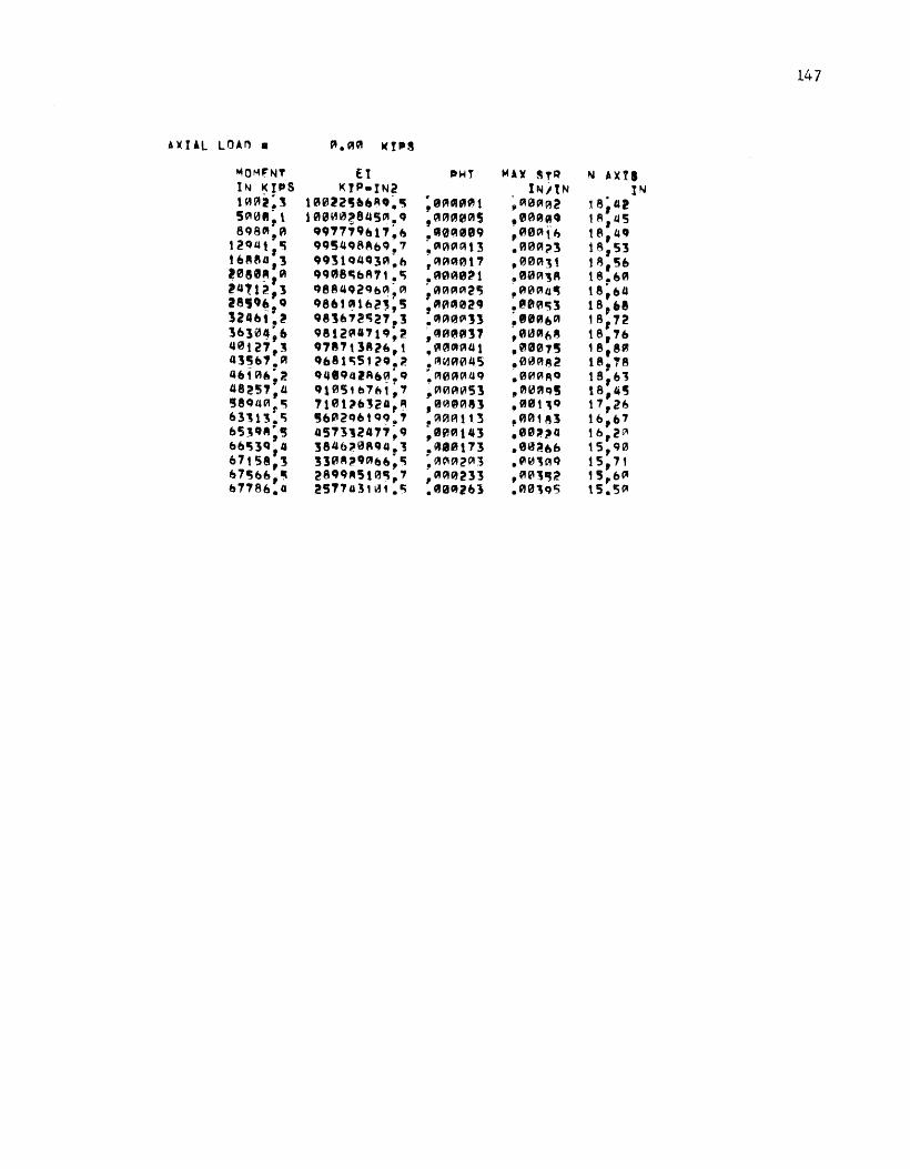
147
AXIAL LOAn a P,.A0 t<ttt8
111QMFNT ft PHT Mi)t ST~ N ~XTS lN I<IPS I<JP•IN2 lN/tN IN 1"~2:3 100~2~'1)R•~rs ;eP!DI919.1t ~010Cll~2 18~tH! 5~0fJ~\ 100t10~81.l50t,.CJ
9 APIPI0PIS • eeu~~ca t~,45 8Q8~.A qc,,779&17~~ ,Q~0QI009 ~0001ft, t8,4'1
t2QUt~l§ 995498~&9,.7 ·"'""'li\13 .0091?3 18,53 U.t~l'll
13 9931Q493A:b ~~AA0t7 ,00PI]1 t8,~b
!080~ 1 A Q908t;b87t~c; .A0"0~1 s00PI,8 t8,.bA '4tti!,l Q881.lCJ2QbQ!~Pl ~!:lJCIIAA2'5 ,.00014~ ts;aa 28··~,Q Q8ftt'!'lb2,,5 ,~~~02CJ .~fl0t;] ta,t:te S24bt,.l 98]b1~t;27,1 ,.Cit00(11]) ~10AbPI ,8,72 lf.tl0~~1:t 98t2Ali'71Q,2 ~ ~ACUJJ? ~00016A 18,7& 40127,] 9787t3R?ft,t 9
91 l,liJ CIH'Il.l 1 ,l'll0'75 te,e~ 43'5b1,.A 9b8t'i5t2CJ.2 .~t1A045 .00AA2 18,78 ~u~'"'"~2 94194ZAb~~Q :A0At:11JQ ~00Cll80 t8 1 b'J 48251,4 9t051b'7nt,7 ~~H'IPllf!53 ,0fcH9~§ t8,45 '38CJIJC'I,.c; 7t0t~o~2~,~ ,90GJ08l .A0t]O 17,26 &3113,.'i 5b02o&t<J<>,., ,00Att:3 ,~HIJ1 Al tb,o7 b5]CU,;5 451l12477~q ,00CI!t43 ·""'-~4 tb,i~ bbt§lQ,IJ 3846~0ACJ4.l .~lftt73 .ee~,.b t5,90 67158,] 3l~A,,Aeb:'i ~OHH~2013 ·"'"'"Q 15,71 &7~&&,~ 28CJq"5l~t;~., ,AA0233 .~~1~2 15,&~ &1786.41 251'7a3t~1.r; ,.CIJ0Gtl6l .A01QS 15.5~
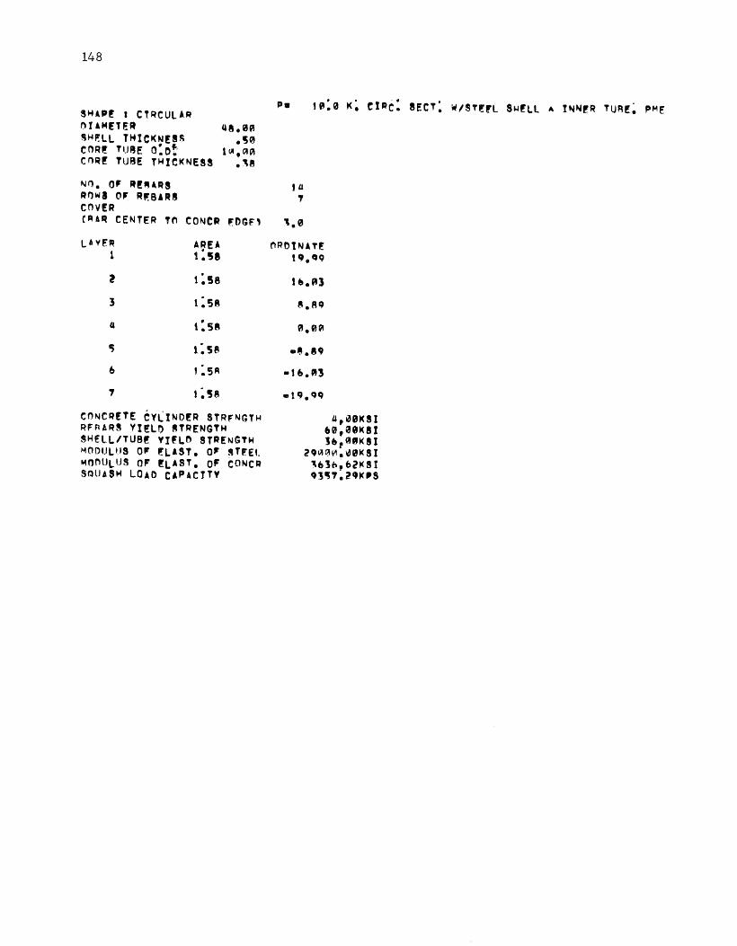
148
SHAP! I CtRCULA~ l'ti U4£TER ~~F.LL THICI<N!S~ cnR! TuBe: o:o~ cnR! TUBE THiet<NE8S
48.00 .1§0
t~,A"'
·"~ NO. 0' R!~ARS ta ROWS 0' RF.BARS 7 COVER C~A~ CENTER Tn CONCR F.DGF' '·0
LAVER AREA 1 t:se
z t:se
3 t:se 4 t: 58
I) t:se 6 t:s~
' t:se
CONCRETE CYLINDER STRfNGTH RF~AR8 Yl!LO ~TRENGTH SHELL/TUB! Vlf.Ln STRENGTH ~~ODULtiS OF !'.LAST • O' ~T~Et. ~Of'ltJLUS OF !LAST. OF CONCA SQUASH LOAD CAPACTTV
a,.aet<si f»0,011<8! Jf),QI&9t<Sl
?Q~00.~01<Sl '&1be&2K8I ~3~7:2'1C'S

149
AXIAL LnAn • 11~A0 I(JPS
"'40M£NT E! PHI MAX !1\T~ N .&lCJS IN I(JtltS ~TP•tN2 IN/IN IN 1q5;~A t8§17'l7~oPI:4 :OI~A~0! " .~001:11~ t'0,3t 5~'51§,! l'H t B28234: ~ ~fi0A0"'5 .000~Q 1~,8! ~"14 ! 1~1]8t3Q&;~2 ,0Pt{lt(lltliQ ~00At6 t8,7t U!~Q,: t QQQ&~01JQ~.~ .~~~(lit] ,A0~~1.1 t8.&A tbQ]'~"' ,,.2Qbtt2,t ,100017 ,0P.IQI'!1 u~;oe 2"'A6~;QI ,.,~,5081.'- ,AtJ~AZt ,00fi'JA 1!,70 24'1&],! QQ0518lf~~; I§ ,et00(11~5 ,0004& 1&,72 28~~.~,,, ~81~pQ&7ft,ft r""'"'"'2q .00&11~3 18,75 12•.u"':§ t8Sl&bA11§~,8 1 00A033 ~A0Aft0 t8,7~ lbJS1.1J '82'5,~!&~,, ,~fUJ01? ~010~8 te,aa 40t7!~8 ,.,.8,Q2c;1.2 .0l'J004t ""'""''~ t! 1 AI§ 436,'Jt,• Q••s~72ll)~4 ~A~0~4S .000~1 18,83 4618t,2 ·4~472b7Q;3 ,G'(IIA049 ~00~8· t8 1 oA 48llCJ,0 CJ120t;7A&Q.I'I ,"~"11!~=51 ~02Aq5 t8,'50 1Jt"'2'•"' 1ttt~Z2~~~01 1 C!JA0083 .~'"''' 1'1,~" &la~&,4 '5otttA'o',• ,QJ0 .. t13 .00t8] 16,71 b54CJ&,• 4SI0it010~,'7 .etawtcaJ ~'''-l5 !6,24 ~bt,3o.R 38'Sl'Pqt!].l ;ee0t'7l .fl0i~1 15 1 Q4 &1250;, 3ltl~40e1~o 1 01PP12Pl3 ,00]t~ t5,.,, &7&58 " 2Q"3121CJ.,,t •"'"'"'213 .~0]tS' 15,&4 b78fHJ=Q ,58 UH341)a • A .80QI2&l .Rl'l,o6 t'i.'55

1.50
9HAI'F t etRCtJLAR niAMETfR S~P.:LI THTCI(NFS~ Cr'!RE TUB!! n:o: enR! TtJ8f THtCI<N!SI
46;0~ . ,50 ,",0~
.]R
NO: OF RI!AAR8 '4 ROWS OF RE~AAS ' env!R teAq C!NTER TO CnNCR EOGFl 1:0
l A V!P. , APE' A t~t;8
ORrHNATE tQ:qQ
~ 1,58
1 t.~e
4 1,5~
c; 1,!~
b t.5A .., 1,58
CONCRET£ CVLI~OER 8TRE~GT~ RERARS YIELD STR!NGTH SH~Ll/TURE VJELD STRENGTH MI')DULUS nF !LAST: OF STEFL Mni')UL!JS nF ElA~T: OF CONr.R SQUASH LnAn eAPAtlTY
A X tAl LOAn • "~~0:0~ KTI'8
MOM!NT EI T ~J l<fi'S KlP•tN~ 1 51$$: 1 !S55tZ?~,Cil;e 7771Jr·~ t!!~0tl91.l9~2,2
1 'JW1T!·a 141.&8~00!~4,7 17/J]A,b t34CII~t~t~1 1 5 2t540~7 t2.7t1211Mlt9.e 2~5~~~.~.~ l21SI§4'JSll~;2 2CJ4~b ~~A ttT'7~7A3~0 1 5 312A0
13 tt47,q&21t,u
37~Q'7t& ttll.lto~?,.,,t IJ~8AJ!b 1 t~4ti&tM114.5 44b'1 1%.1 t0eAii&l8G7;3 483~2l8 t6Y4~G!~3i,l.8 5~1i!lllj4,~5 !0621]'74~tJ;?. 552"tT.·e t041t;28943,2 &62A!t-7 7'1fal94l7 1 8 7~8AS ·s &~'110~att&,s 11tt1,1b 511~819$3,~ 741 ~ft'·-8 42,_418~tt,t 74396!~ 36oa82T15.8
tb:~3
A:89
4,08kST M~,C:I9fU<ST
3b,061CS! 290AI!1,00k8T 3ele •• l~<IT Q351~!QI<PS
PHI MA)( STR TN/IN
;000A01 ;et~~t3 1 fUIUH'H~§ ,9~~'3 ,ra~~"'rac, ,00~32 .~~ACIIl3 1 0PA40 ;"-100011 ,eAe4e 1 A~~~2t .0~1'!1:;6
,~0"'025 ;0"'A64 ,~f'I002G 1 A0P1'71 ,0~01t]3 1
01'1A'7q 1
1'1AQIA]'7 1 11'ftAA7
1 AClll"041 ,00~Q5 ,0a0045 ,0QI~_02 ,0A0Clii4G 1 0Att0 '(l!(l!f105l ,00!18 •"'"'e-983 ,~0171
1 1iHHHt3 ,01'1223
1 1Ut0t43 ,002'77 ,cHUJt73 ,0~1]0 ·"OJ~lA3 .0fl,84
N A)(tS TN
t34~'5~ 4~,23 3'5,~b 31.3~ 2~.80 27.t'S 2111j,QQ
z~.t" 24~50 24~00 23~~9 21.1& 23~00 22,7~ 21~~'7 20.~6 1Q,84 1q,5'7 !0~19
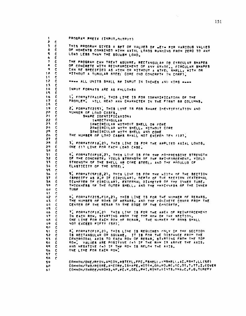
t ~ ~ ] c Q e ~ c & c 1 c ~ c: q e
\~ c t ' e 1() c t' c 14 c tlli c \~ c: , '7 c: ~~ ~ tQ c: ?111 ~ ?1 c 22 e e' c ~ll c 21i e 2b c 21 c ;u~ e 2Q c 'JQI ~ 1\ c ~2 c
'" c 14 c ,c; c ~f) c ]'7 c !A c "Q r. Ul!l c l&1 c 42 r: 4J c U I! c iJS c 4b c IJ 7 c 4P, c tJQ c c; '~ ~ ~t c 1§2 c ~' c ~a c r;c; c '5& c '57 c 'SA c 5Q e"' b1
Pltnr;R AM ttME t )( C t NlttJT, n11TPUT l
TMTS PRO~RAM GIVES A S'-T 0' VALU!8 0, .[T• 'OR VARIOUS VALUES 0' MOM!NTI eoMRiN!O WITM AXTAl Ln40S RAN~INr. F~OM l!RO TO ANV LOAn LESS THA~ THE SQU~IH LOAD~
THF. PROGRAM CAN TREAT ~QUA~!, R!CTANGULAO OR CTRCULAR S~AP!S 0' CONCR!TE WITH REtN,nRCEM!NT OF ANY ~RAO~:. CIRCULAR SHAP~S CAN RF SP!CI'lfD AS ~tTH OR WITHOUT A 8T~EL ~H~LL1 WITH nR WfTHnUT A TU~ULAR STE~t CORE (NO CON~RFT~ JN CnRF):
•••• ALL UNITS SHALL A~ INPUT IN !NC~EA ANO KTPS ••••
INPUT fi'OR!o4ATS AR! AS F"LLOwS•
1: FOR~4TtAAt0l: THIS LIN! tS ,OA tO,NT!~tCATtnN OF T~f PRORL!M: WILL REA~ ANV CHARACTER tN TH£ FTR~T 8a COLUMNS.
2: fi'ORMAT(2t5l: THIS LTNf TS 'OR S~AP'- I~E~T!FTr.ATTON AND NUM8ER O' LOAD CASFS.
S~A-~ ID~NTIFICAT!ONI t a~!CT4NGULUt
10aetRCULAR WtTHOUT SH!LL OR rOgf 21'.1sCIRCULAR WTTH SHELL• 114tTHOIIT COR! J~•CIRCULAR WtT~ SHELL AND eOR!
THF. NUM8!R OF LOAD CAS~S 8HALL NOT EYCFE~ t~~ f\0):
3: ~ORMAT(Ft0:2\. TH!8 LINE II FOR THF. APPLTED AXIAL LOADS. ON~ (1\ LIN~ FOR ~AC~ ~OAO CASE~
4: ~OR~ATC4~t0:2'• T~t~ LYNF IS Fn~ TH, ~OMP~ESSYVf STRENGT~ OF TH~ CONCR!T!, YTEL~ STR~NGTH OF T~P.' R~t~FORCEMENT, VtfLO STRF.Nr,TH OF TH! S~FLL nR CnR! STf!L, A~D T~f MnOULUS OF ELASTtCt1V O' THE STE~L:
5: 'ORMAT(~Ft0.Zl. THY~ LINF !S FOQ TH~ wlDT~ ~F THf SECTION t S P £ C IF V A 8 0 : ~ t F C I R C U L A~ ) , ~Eft T H 0 F -T IJ ~ ~ ~ C T t 0 N t r!" )( T 1!: RNA l DtA~F.T!R Jlf CIRCULAR),. !)(TF.RNAL DtAMfT'R C, THF t"JN!R TUBE, THftKNf8S ~F THE OUTED SHELL, ANO TH! vMTC~~~S~ nF THE INNER TlJBP.'
e: FORHATt;:!t5,F1~.Zl. THIS LIN! TS FOR Tlo4P: NIJM~E~ nF R[fURS, THf NUMBE~ nF RO~S OF ~!RARS, A~D TH~ rO~C~ETE CnVFR FROM TH! C!~TER 0' T~E REeAR TO TH! EDG! nF TH! C~~r.R~TF:
1: FORM4TCFtA:2l THIS L!NF IS FOR T~! A~EA O' Rf!NFORC!M!NT IN EAeH RnW~ STARTING ,ROM THf TO~ RMW 0~ THF. ~feTyo~. O~E' ttN[ FO~ EACH ROW nF ~ERARc T~F! NttMP.!~ t"'F ROWS SHALL ~OT F!XC!!D FtFTV t50>:
~: FORMATCFt~~~l. THIS LINE IS ~~QIJTR!n ~N~V IF THF SECTION IS RECTANGULAR OR SQUA~!. JT II FOR THE ~ISTANC~ FROM THf CF.NTROJDAL A~IS TO F!ACH ROW OF R!8&R; 8TARTT~G FROM THF TOP Ra~: VALUfS ARE POS!TTVE (+' IF THE RnW I~ ARnV~ T~~ A~IS, AND N~GATlV£ (e) IF THF RO~ IS RF.L~~ THE A~tS. nNE LTN[ 'nR EAC~ Raw:
151
COM~ON/0Nf/~r0~ 1 AMCON,~ST~~L,,FC,PS~~Lt ,AMSH!li_,AC,PSHT,LLC50l COM~ON/TWOIPCOR! 1 AMC0Rf,lS~AP!,Wt0TH~On,~O,RC,nC,DT,T,TT,z,eOVER COMMON/T~R~E/NR0WS,NP,FC.k 1 D!L 1 PH!,RtNT,Rt~TS,nNA,C,F,G,TUREFV

152
b? COMMON/,OURIMA,t!,~K,PeAP,~CS,ROS,RT,RfS.OIF,ASHCt~~),tJ,PCT,NBARS ~' COM~nNIFtVFJPft0l,ASt~~,,xsc50\,SS~f50''qS~t~0','x~r~~,,~,R,V,sTR 64 C~~~ONISiXIXt190,,CSNt\0~\,CSift~0\,Aeef10~\,ATOT(t~~l,SSMCt00) ~~ CO~MnNIS!V£N/~SSHCtA0),xxctee\,Rxxct~~''AMr5~,,xxsct~~'•Rxxsct~~' h~ COMM0N/!tGHT/TAtl0~'•RTACt~0l,TACCtt00''oACCC1~0l,RXtt~~),ES,EC,I~ b1 CO~MON/NtNF/PASHCtA0\,~ATOT(l00\,RTOff10~),RTACCf1~~l,TOTC1A0) ~R DI~ENRION ANAM~(8' ~Q DJMFNS!ON D~NAC2\ 7~ REAL NONA 71 R!AD 20,tANAMECil,t•!,~\ 7~ R!An t,tSHAPE,NP 1] R~AD 2 1 (PtJ\,Jzt,NP\ 1~ R!An l,~C,RA~FV,TUREFV;!S 75 ~!AD Q,WJDTH,OOtOT,T,TT 7~ PRINT 2!,tANA~E(!),lat;A\ 77 IF CISHAPE.~~.\) GnTO iA 78 PRINT b,OD,T,OT,TT 7~ GOTn tq R~ 18 PRINT 7,WYOTH,OO ~t tQ CALL SETUP R?. PRtNT 5~N86RS A~ PRINT R1 NROWS ~4 PRINT tt,cnv!R A~ PRINT q A& PRtNT t0,LJJ,AStJ,O.,XStJJ\,JJat,N~nws, A1 PRINT t2,FC AA PRINT 13 1 8ARFV AQ PR!NT Ut,TURE'FY Q~ PRINT 1~ 1 FS Q1 PRINT tb,EC q2 PRINT 11,PCiP q1 D~ ~~~ Jat,NP qa IF tPrAP.J'If.O' 1.4:J"',26.)& q~ 2b PRINT l0,P(J, qb PRtNY 2t q7 PRTNT ?3 QR PHta.0000~1 qq '5 NSWTC~•9
1~~ DONA(tl•0:~ 1~1 00NAt2'•0~ t~~ ONA•OD 101 a0 CALL CSTqE~~ 1~4 PCOND0 0 ~ 1A5 IF tDNA•OD) 33,33,55 1~& 33 ~•INTCONA/D~L) t~1 GO Tn IJSt t~8 S'5 KSb0 t~q 481 CONTtNU! 11~ 00 Q0 Iet,K 1t1 XXCJ)•XCJ,+RO•nNA 112 1' ttSHAP!~~~.t) GOTO A5 \1, XXStt\•X~fi'*XX(Il 111J tF CRtNT;GF.:A~SCXXCt''' GOTn IJ7 tt~ ACCCt\a~.A i1b GOTO aa 117 47 ACCtt)a2:*~~RTtR!NTS•X~S(f''*D'-L 11A U4 PCONaPCON+CS8Ct~•ACCCT' 11q GOTn q~
12~ 85 PCON•PCON+AC•CSSfl) 1?1 q0 CONTINU! 122 CALL AT~f.LP 1~1 PTOT•PCON+~STE!L
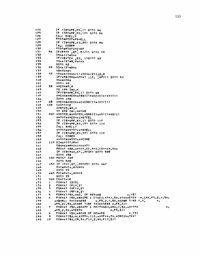
t~IJ
t~'i
t2b 1~'7
t~A t2Q t1"' \ J t t~2 111
'~" 'Jlli ,,b tl7 ,,~
1JQ HJ0 tat tat» 14, 14U 14~
HJb t47 t IJP taq tl:i~
tl:it 1Ci2 p;, p;a ,.,c; 1-;ft 1~7 1CiA tSQ th" t n 1 tb2 11)\ \!',lJ tbl:i
'~~ 1~7 InA tbQ t7c.i
' ., t t1? t73 t71J t1Ci ,.,, ,,, t'7A t7Q lAr.\ t A 1 tA2 pn tAll tR'i
I~ tiSHAP!~'~:tl GOTO ~b JF tT~HAP~~'~.t~l GOT~ An CALL SHELLP PTnT•PTOT+P8~fLL IF tlSHAP!.fQ:20~ GOTO ~b CALL COR~P PTnTaPTOT+PCnRF
~b IFfPTnT ~GT: PtJll GnTn RQ OI'Ha ttl 81')N A JFtNSWTCH .~Q: llGnTn Q2 OI)N A ( ;t \85: f.'l•rPH GOTO Q2
RQ DDNAt2'•0NA N8WTCHa1
q2 NONA:tDDNACtl+DONAt2,l/2e0 IFtA~6CDNA•NnNAl .L~. :~f.'l~1l GnTn ~~ DNAwNONA GOT 11 U0
5&9 AMCON•91:A 00 t00 t•J,K. IFtYSHAP!.F.~.t\ GOTn 611i AMC~N•AMCON+CSSCil•ACCttl•tX~CTl\ COTn 1""0
b5 AMCON8A~CON+AC•CS8t!l•r~~ttll t "'" CONT! ~liE
A~S'TE'EL•0: r-1 00 2A0 !•1 1 N~OIII8
~0~ AMST~!L•AM,T~~L+SSSfll•ASfil*XSttl AM'TOTaAMCON+AMSTFEL IF ttSHAP'-~F.q:t~ GOTO '1P IF tiSHAPE.£~.10' GOTn tt~ CALL SH~I.L"' •MTOT•AMTOT+AMS~ELL IF tt8HAPE~EQ~~0l GnTo 11P. CAll CORF.M AMTOTaA~TOT+AMCORE
t1A EI•AMTOT/PHT CSNMAX•PHI•tnNA•T' PRtNT iJ00,AMTOT,EJ,PHY;csNMAX,nNA IF tCSNMAX.r.r::0~3A' GnTO ~~0 GOTO 4159
41" PRTNT QQ" GQTO 1HHl
4~~ IF (PH1:Gr::~~~~5' GOTn 4~~ PH T •PH t + ~ 0i~L~c;!~l.l GOTO ~5
iJb~ PHJaPHT+~0~~~l GOTn 1'5
S~~ CONTtNU'-1 FORMAT t2T'5l 2 FORMAT (Ft~:2l ~ FORM•T t4F1~~2l ~ FORMAT t~F10:2' 5 FORMATf~X,•NO: OF REBARS •rT5' 6 FORMAT t~X,•SHAPE CT~CULAR*I,SXr*nTAMETER
•*SHfi!LL THTCKNE~S .;,as~2,1,5x,•cortP.: TIIR!' •FIJ:2/,~X,•r.ORF. TUSF. THtCI<Nfi!SS •,F'5~?1'
7 ~ORMAT t~X,•SHAPF I RFrTA~GULAR• 1 1 1 5~,*W'OT~ •F5~2 1 '5X,•n€PTH *rF'5~~/l
~ FORMAT f5X,•ROWS OF ~F.~&RS •,I5l Q FORMATC~X,•LAV~R•,ttX,•ARFA•r7X,•ORDYNATF*'
t~ FOR~ATf~X,I~,~X,Ft~:2,~~,Ft~.2/,
153
•,t(;IX 1 F~.2,1,'5Xr n.n: *• .,
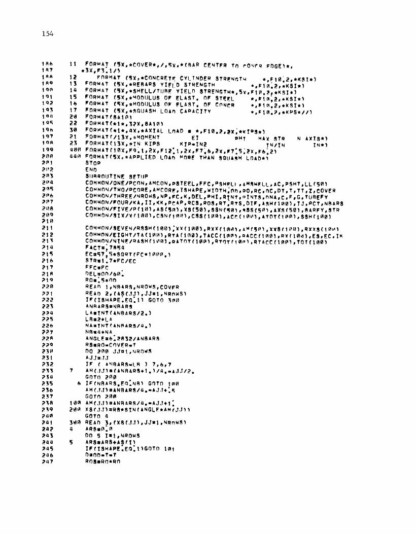
154
!A~ 11 ,OR~AT f~~.•COVER•,I,~~.*CAAR C~NTFR Tn rO~rq FDGE'*• !R1 •lX,,~:tl' fAA 12 'O~MAT (~X,•CONCR~T~ CVLTNOER STR~N~T~ •,Ft0:2,•KSI•) 1AO 13 F'O~HUT C5ll,•REB4RS VIFtO STREt~~GT~ • 1 F1(:'1:2 1 •KSl•l tqCJI 14 FORMAT C~X,•S~E'LL/TLJA~ VlELn STREN(;Tio<4•,'5'li',FtP-.~ 1 •1<Sit) 1Q1 15 FORMAT t!X,.~ODULUS OF £LAST. OF ST!~l *•'t~:2,•KSI•' 1Q2 tc 'ORMAT tt;X,•MOOIJLUS OJi" FLAST. OF CMJeR •,lf1~~2,•1<SI•l tQ3 17 FORMAT (~X,•~~UAS~ LOAn CAPACJTV •,Fl"'~~•*I<~S*//l tQ4 2~ FQRMATt8A1~' tQ~ 22 FORMATt•tw,]?X 1 8At~l tQ~ 30 FORMATC•t•,4X,•AXJAL LnAO • •,Ft0.1,,x;•~t~!•l tq1 ~1 ~ORM4Tf/13X~*MOMENT ET ~~T MA~ sTq N AXlS*l 1qA 21 FORMAT(t]X,•YN KlPS K!~•IN2 TNI!N IN*) 1QQ ~~~ F0RMAT(t~~.~Q:t,2X,F12:t,2-,F7~&,2X,F7:5;~x,F&:2l ~~~ 44~ FORMATt5Xo*~PPLigo LOAn MOR~ T~AN SQUA~H lOAO*' 2CJI! STOP 2t-'1;? ENI')
2Cill3 SUio'H~OUT!NF. S~TIIP
2~4 COMMON/ONE/PCON,AMCON,PSTEEL,FFC,PS~FLI ,,~~~,LL,AC,PSHT,LLtS~l ~~~ CQMMO~/TWO/PCORE,AMCOR~,!S~AP!,WIOT~~o~,pO,RC,nC,DT,T,TT,Z,COV~R ?P~ COMMON/THRE~INROWS,NP,~c,K,OfL,~Ht,RtNT,ot~Ts,nNA,c,F,G,TUBEFV 2~1 COMMON/,OUR/KA,II,K~,~eiP,RCS,ROS,RT;RTS.OI~,AS~t1~0l,TJ,PCT,N8ARS ?~8 COMMON/FtV~IPtt0l,ASC~~l,~SC50l,SSNt~~l,-SSC5~'•'XSt50l,AARFV,STR ~0Q COMM0NIS!X/Xft~~l,CSNt1A~l,C8SCt~~l,AC~(10~l,ATOTtt~~l,SSHtt~0) ~10
211 COMMON/SEV~NIR8SHtt00l;X~(1~0),RXX(1~~,,AMt~~l,XWStt~0l,RXXSCt~~l 212 COMMnNI!tGHT/TA(l~~l,RTAttA0),TACCtt~~,,o,cert"'0l,RVtt0~l,ES,EC,JK 21~ COMMONINt~~/RASHtt~~),qATOT(t~~,,RT~Tf1~~,,RTACCt1~~,,TOTC100l '14 FACT•:78~Q ~~~ ECa~7;5•SQRTtFC•t~~~., ?tb STR•t.7•FC/EC ?11 FFCaFC ?.tA 0ELaOnlb0: '1~ Roa:5•0~ 2?0 REAn t,NAARS,NROWS,COVFR ~?1 READ 2,CASCJJ,,JJat,NAnWS' '22 l'CISHAPE:~~:t, GOTO l~~ ~2~ lNRA~SaNRARS
~~4 lA•tNTt4NBAR512el ?25 LB•2•LA 22b NAaTNTf.ANRAR514•' ~?7 NA•4*NA 22A ANGLF.•6:~81~1ANBARS ??Q RSaRO•COVER•T 21~ DO 2~0 JJat,NRn~~ ~3t AJJsJJ ?~2 IF ( A~BARS·LR ) 7,6,7 ? :\ 1 7 A N t .f J \ a ( A N FU R S + t • l I /.J • • a ,J J I 2 • 214 GOTO 2~~ ~35 & IF(NRARS~~~:NA' G~Tn t~H 2 'J b A M ( , T ,J ' ca AN BARS It.& • • A J, f + : e; 2~1 Gorn ?.~~
f)' 8 t 0 C4 AM (.f ,J\ II AN R ~ R S I tl ~ • A J ,J + 1 : ?'q 201o'l! XSfJJ):uRS•StNtANGLF•AMrJ~T'' ?4A GOTO Q ?4t 3~A REAn l,fXStJJl,JJ•l,NRnWS' 24? 4 ARSaA:~ ~41 00 5 I•t,NROWS ~aa 5 AAS•ARS+ASft' ~4~ IFtiSHAPE:E~:tlGOTO 1~1 24& DanO•T•T '-41 AOSaRO•Rn
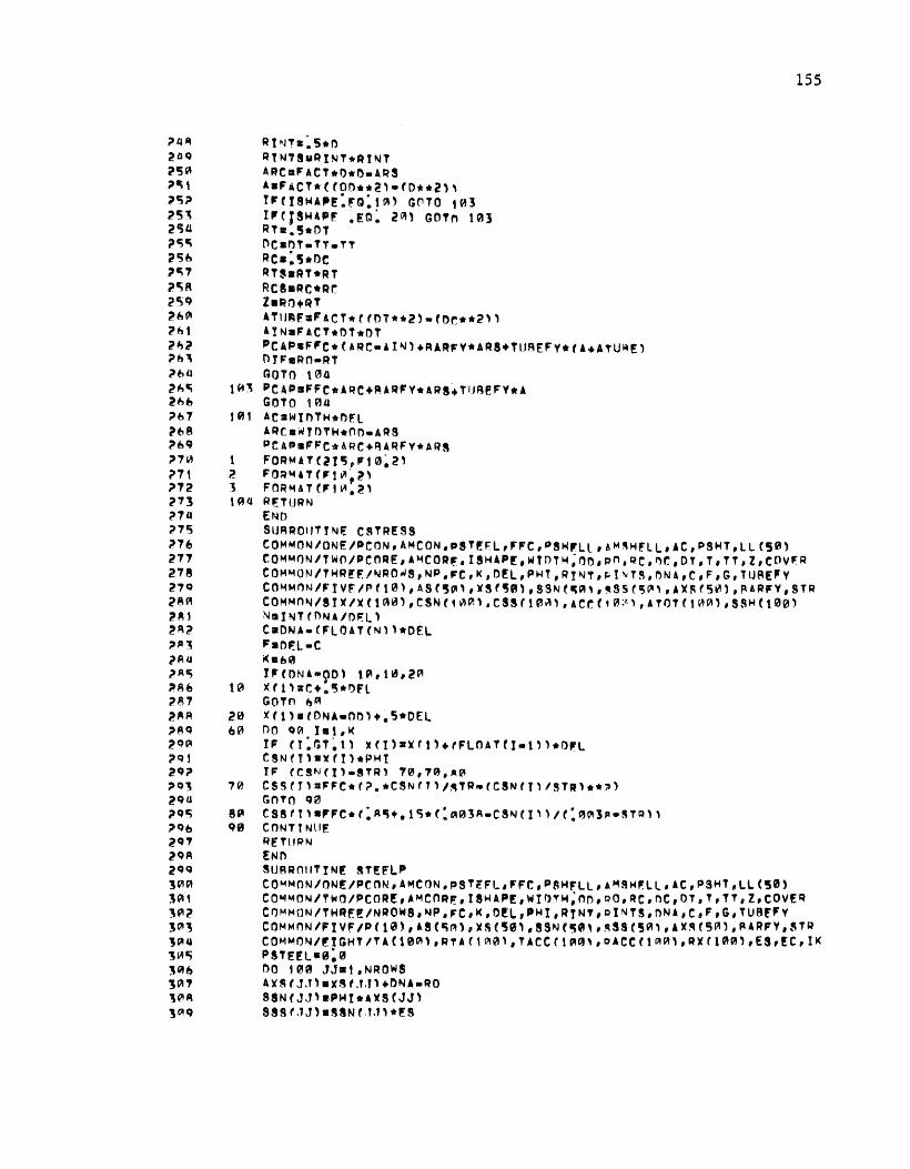
i'4~
2lJQ i'15~
~~\
i'"i~
25' 215tl i?c;Ci 215~ 11;'7 ~r;R
2'5Q 2~!'1
t'ht 21,? ~h' 2b4 ?.~"i 2~1t
i'~1
2b8 ;:tt,Q i'1VI ?7t >'72 273 ?74 ?'7'5 ,..,& 277 2'78 27Q ?API t>A1 2A2 ;:tP" ?Ata ;>Ar; ~R& ?R1 2AA )~Q
21!i1A ;:tQ1 2Q~
)Q~
2QU 2Qr; ;:tQb
2Q'1 2QA 2QQ
3""' '"', 3~2 ]01:\
JPI'l ]VIr;
]A&
3"'' JCIR ]rJIQ
20 o0
Rt~JTz:s.n RtNTSuRt~T•RtN'T
ARC •F A CT• "*"• U~! A•FiCT•((00••2'•tD••2l' t'fi8~A~E:~Q:t~l G~TO t~l IFCJS~APF .EQ: 2~l GOTn 101 RT•.5•DT l"lCaOT•TT.TT Rc•:'5.oe ~T!aRT•RT RC8•RC*RI': Z•RO+QT ATIJ~Fa~FACT1t t rf'1**iD•fOr.••2'' A!NaFACT•nT•OT . ~'CAP•FFC•fAQC•AlN~•RARFV*ARS+TUREFV•tA+AtU~!' nn:·•RO•RT GQTO t\'Jll PC4PsFFC•ARC+RA~FV•ARS+TURfFV•A GOTO t P.ll& AC:aWtDT~•DP:L A~C•wTOTH•OO•ARS PCA~sFFC•ARC+~ARFY*AR8 FORMATC2t~ 1 F10~2l FO~M&Tllf1VI~2' FOR~ATflfJ~,2' ~~TURN ENt}
155
SURROIIT t NF.: CS TRESS COMMnNIONF-/PCON,AMCON,pSTfFL,FFC,PS~,LL,AM~HF.LL,AC,PSHT,LLC50) COMMON/TwO/PCO~E,AMCOR~,ISHAP!,WTDTH;~~~pn,QC,~C,DT,T,TT,l,COV~~ COMMON/T~R!F.INRO~S,NP,FC,k,Ofl,PHT,Ry~T,~I~T~,nNA,C,F,G,TU~E'V CnMMnNIFIVFI~tt0',ASt5~''~9t~~,,SSNt~~,,~ssr~~'''x~rs~l,~ARFY,sTR COMMO~ISJX/XC1A~l,CSN(1~~,,CSSft0~l,ACef,0:,,,ATOTt1~~),SS~Ct00l NstNTtnNA/DF.ll C•ONA•(FLOATCNll•DEL FaDP.:L•C 1<•&0 JFCDNl•90l t~,t~,2~ X t 1 h: r. +. '5 * l')f l GOTn fJA Xttl•CDNA•OD,+,5•0El no QQI Ist,~<
IF tt:GT~tl ~tt)aXttl+rFLOATti•tll•D,L CSNftl•Xtll•PHI IF CCSNftl•8TR' 70,79,~~ CSStf,aFFC•t?.•CSNfTl/~TR•tCSNtt,ISTRl•*'' GOTO qe CS8ttl•FFC•r:A~+.15•C:~03A•CSNCI'~If:0~l~•ST~'' CONTtNllf: RETIIRN !Nn SURROIITINE STEP'LP co~MONION!/PcnN,AMCON,PSTlFL,,Fc,P~HFLL••~sH~LL,AC,PSHT,LLC50) CO~MONITWO/PCOR!,AMCORF,IS~AP[,WI~~~~OO,QO,~C,nC,DT,T,TT,Z,COVEQ COMMONITHRF.!/NROWS,NP,FC,K,O!L,,Ml,RTNT,~INTS,nNA,C,F,G,TUBEFV COMMnNIFtVFIPfl0l,AS(~~l,XS(50l,SSNC~0,.~ssc5~'''x~c5~),RARFV,STR COMMONI'-!GHT/TA(10~~,RTA(1~0l,TACC(tA0,,gACCtt~~,,RXf10~~,ES,!C,Ik
PSTE!L•9;0 DO 100 JJ•t,NROWS A X~ r J J) •XS t .Y.O +DNA•RO SSNtJJ'•P~t•A~SCJJ) SSS r .TJ) •~SN r .Y.J' •F.S
156
'1 ~ I I' ( S S S LJ.Jl ; G T 9 BARF V) ~ S S C J J) • RAP F V ~ti IF tS~SrJn .. LT.•BAPF''n SSS(JJl••FUP,y 1 t 2 ~ 8 T E' F. l :cPS T F.~ l + A ~ ( J J l * ~ ~ S t ,f .J \ :41~ ~~~ CONT!Nll! 'ttl R!!TtiR-N 11'5 EN" Jtt. SUFH?niJTtNE SHELLP 3t7 COMMON/ONE/~CON,AM~ON,PST~~L,~'C,PS~~ll 1 AM8~FLL 1 AC,PSHT,LLC50) ]1A COMMnNITWn/PCO~E,AMC0~£,!3HAPE,~TOTH;on,~O,~r.,~C,DT,T,TT.Z,C0VEP ''q CO~MON/THREF./NPOWS,NP,~C,W,D~L,PHI,RtNT,PINT~,"NA,C,F,G,TlJB!,V 12~ COMMONI,OtJPi~A,It,KK,PeAP,~CS,Ro~,PT,RTS,otF,As~ct~~,,IJ,PCT,N~A~S 3~1 COMMON/,tVF/P(10l,ASC~~l,XSt50l,~SNC~~''~SSt~0',A~Sf5~l,BAR,V,ST~ ~2~ tOMMON/S!XIXtt00l,csNtt00l,C3SftAJl,Acrt1~~,,ATOTtt~0l,SSHCt00l '?' COMMON/8EVF'N/RS8Hf1~0l;xxtt00,,RXXCt~Al,AM(5~l,XXStt0~l,PXXSft~~l l2a COM~ON/EfGHT/TAC10~),PTA(t~A),TACCtt~A,,oAecr1~0l,RX(1~0l,ES,EC,!K 125 COMMON/NYNE/P.ASHC1~0),RATOTC100l,RTOTtt0~l,pfArCti~0\,TOTt1~~) ~2~ DIM~NAlON ~Mt1~0, 127 PSHT•~.e ,?~ P$HELLB~~~
~2q no 103 I•t,K lJ~ I, CRO.GT:Ae8tXX(lll, ~OTO 110 ,3! ASHtf\m~~0 112 GOTO tAb 113 ttA AiOTttlal:*S~RT(ROS•XX~CT,l•OEL 11~ ASHCt,:ATOTCil•ACCtl) 33~ t0~ SS~ttl=!B•C8Nttl 116 !F CSSHti,,GT~TURE~¥) ~SHC!l•TUqFFV ~37 IF rSSH(t,.t.f.oTUBFFY\ SS..,Cil••TIIBFFV JJA 20] PSHF-LLSP8HELL+ASHCil•S~HCil ~lQ IF ro~A-on, t~7.t05,t~~ lU~ 1~7 KAm~q.K
~41 Do t~a rwt,KA 14? RXti)sXCI'•C+F 14] RXXfll3R~·nNA•RXCI~ 1~4 RXX8f!)aRXXCil•RXXC!l ,4~ TF CRT~T:GT:ARSCRXXCill\ GnTO 47 3ab RACCC!la0:~ '~7 r.oTo 44 108 47 RACCtYla2~•qQRTfRINTSo~XXStlll•D~L ]Qq aa I~ tRO.GT~ARSf~XXfTl)) GOTO 45 3~~ RASHCilue.~ 1~1 GOTO t04 3~2 48 RATOTri)u2.*SQRT(ROS•~XXSti1l•DEL 1~, RASHCTlu~•TnTCil~RACCtT' 'sa SMttlmRXtYl•PH! '~~ RSSHtils~S•S~CJ' 1\!Sb !F fRS$H(t1;r,T~TIJREFVl ~SSHtJ)~:TIJ8F.'¥ 15'1 IF fRF;~HtT'.LT .. •TURE~V' f:(S~H(f)••TII!=tFFV 1~A 10b PSHTaPSHTtPASH(I'•RSS~tY' ~~q GmF•~~!•F.S•T•DEL 36~ P$HELL=P8~Fll•PSHT•G 361 ttl'S R~TURN ,b?. !ND 1~3 SURR~UTtN! SH~LLM ]ba COMMON/ONEIPCON,AMCON,PSTEEL,FFC,PS~~Ll•A~~HELL,AC,PSHT,LlC5~l 3b5 COMMON/TWO/PCOREBAMCOR~,JSHAP!,WtOT~,nn,PO,RC,~C,OT,T,TT,Z,cOVER 3bb CO~MONITH~F~/NROWS,NP,FC,K,n!L,PHt,RTNT,Pt~T!,nNA,C,F,G,TU8fFV ]~7 co~MON/FnURIKA,I!,KK,PrAP,~CS,Rn~.QT;Rr8;ntF,A5HttP~l,IJ,PCT,N~ARS ]bA COMMO~/,tV~/Pt10,,ASC5~l,XSC5~),SSNt~A''~SSr5~l,AXSC5~l,RARFY,STR ~bq COMMON/SIXI~t100l,CSNtt~0,,CSStt~0l,ACrt10~l,.TOTCt0~l,SSHCt0~) l7A C0MMON/8FVENIRS!Htt~~l,XX(10Al,R~Xft~~l,AM(50l,XXStt00),RXXS(t~~) ]7t CO~MON/~!GHT/TAl10~),pTA(1~0),TACCrt~A,,cACCt1~0,,RX(1~~,,E3,EC,IK

]72 ,7~
174 ]7~
17b ]11 17A '\7CJ 'HU~
3Rt 1~2
'R' lR4 1R&; lA& ]87 ]AA ,~4
,~121
]~1
~Q2
]Q] lQ4 1Q~
:JCJo ]Q1 ]QA '\CJq IJ(l!A
/JOlt 40~
4WJ i.l~JJ
JJ(ltl§
lJ"'b 4~1
t11i18
4"Q 41'~
Itt t 41~
413 Ut4 4111i 1'.11~
1.1!1 41A U1CJ 420 4 ;.» 1 422 421 424 IJ2c; 42& IJ21 42A 4?CJ 4,0 ll]\ 1.112 43]
157
CO~~nN/Nt~E/~ASHt1~0l,~ATnTt10~l,RTOTt'0~l,~~ACCft~"'1,TOTC100l AM8HELL•~:~ t.~SHT•0:~ DO 1~0 Tat,l<
lP.~ AMSHELL=A~SHFLL+SSHfl\•AS~ttl•~Xtt\ I, tONA•OD\ 4~~~~02,&A~
49~ DO ~~1 I•t,KA 59\ AM8HT•AMS~T+RSS~(l\*RA~H(I\•CRX(f~+O~A.~nl SA~ AMSH~LL•AMSHELL+AMS~T+~*fFI~,+DNA•Rn~ &00 RETURN
END SUA~O!JT HJF! CORF ~ CO~MO~/ONE/PCON,AMCON,~STEEL,~FC,~SHFLL 1 AMSHfLL,AC,PSHT,LLC50\ COMMONITWO/PCORE,AMCOR~,IS~APE,WTDT~;nn,~O,RC,~C,DT,T,TT,l,COVF.R COMMON/THRFE/N~OWS,NP,FC,K,DEL,PHI,RTNT,QI~TS,ONA,C,F,G,TUBEFV COMMONI,OIJR/I<A,II,1<1< 1 ~rAP,RCS,~OS,~T~RTS;~tF,ASHf100),tJ,~CT,NRA~S COMMON/F!VE/Pft0),AS(~~\,~SC50) 1 SSNt~0\ 1 ~8St50\,AXSt5A),8ARFY,STR COM~0~/9JX/~(1~0),CSNt1A~\,CSStt~0\,4CC(100),ATOTft~~l,S~~r.t~01 COMM0~/8!VFN/RSSH(100\;XXCt0~\,~XXCl~~\,AMt~~\,~XSCt~0\,RXXS(100) COM~ONI!IGHT/TACt00),RTACt~~l,TACCrt~A\,~ACCrt~0\,RXft00\,ES,FC,II< COMMON/NJNE/~ASH(100),QATQT(t00),RTOTC10~),RTA~CC10~),T0Tf100\ COMMONITEN/NN,S(\00l,CqT(t~~\,CRt1~0\,~(1~~\,Rr.Xtt~~l C 0 M M 0 N IE l ~ V F ~ I C X t 1 ~ 0 ) • q N C t ~A ) , C S t 1 ~ QJ \ , ~ r 1 ~ ~~ l , R ~ t 1 A 01 l CD!L•nT/~0~ NN•tNTfONA/C~F.:L\ CC•n~A•FLOATtNNl•CO!L CF•CO'-L•CC !Ft~NA•l\1~,1~,20
10 CXt1\•CC+:~•CD£L GOTO &"10
20 CXft\•(DNA•l\+~5•CnEL &010 on~~ t•t,10~
!FCt~GT:t\ CXCtlcCXt1\+ffw1l•C~!L SNtT\:CXfT'*~'~I CST t l \ •ES•~N rt l IFfCSTC!l~GT~TU8EFV) CqTtt\=TU~!FY !FCr.STCt\.LT.•TUREFV) rSTti\a•TUREFV
ql'! Cr:lNTINIJE c::tcT·~·" . . PCOREaf?J.C'I IF(ONA•Z\ 1,1,5
1 IFtDNAwOJF\ A" 1 80,4 4 lK•TNTf(ONA·~T,l/CD~L\
GOTCI l't
CJ I K•20! & 00 70 t•t,II<
CAtTl•CXtt\+~O·DNA CSCtl•CR(t'•r.BCt' lFt~T•AR~tCAtT'l\ 1~,t~,2~
15 TOTti,•Gll.~ GOTn 10
2! TOTfi\a2:•SQRT(RTS•r.Stt\\•CnEL 30 tF tRC•AAStCAtTll\ UA,Q0,5A 40 TACCCt,a0:~
GOTO &9 5~ TACCtt'•2:*8QRTCRC~•CStt''•CDF.L &0 TAtt)•TOTCI'•TACCtil 1A PCOR!•PCOR£+TACl\*CSTtT'
IFCDNA•Z, @0 1 2~0,20~ 8~ KK•INT(tZ•D~A\/CDEL'
T'tONA•DtF\ ~~,10~,100 qs RCXttl•OIF•ONA•.~•CDEL
158
a'" l(l(a20 4]~ GOTO Q~
n16 1~~ RC~tt,•eF+c'*CnEL 4,1 K~atNT(tl•ONAl/COEL' 43A q~ 00 18~ I=t,KK IJ3Q IFCT.GT:tl RCXttlaRCXt1'+tl•ll•COEL 44~ Bti'•Rn.nNA~RCXt!' 44t RSttlaBttl•Atl' 44~ IFCRT••~stArtl'l t~0,t~0,t]0 IJb~ l2~ RTOTttl=0:0 444 GOTO t4~
aa~ ~~~ RTnTti~=2:•SQRT!RTS•8Sri'l*CDEL QIJ~ 140 tFCRC~ARSCRti\'l 150,t~~,t~~ 441 tSe RTACC!ll•0.P 44A GOTn 17~
4«0 ~~~ RTACCtil•2~•SQRTCRCS•Rqf!'l*CDEL USA 17~ QTAtll•RTOTtilwRTACC(t' 4~1 H(Il•CSTCtl•RC~ttl/C~fT\ 4'5? IF CI·H I l ~ GT ~ TUAF.:FV ~ IH J \ •TtJAEFV 415] IFCHCt)~LT~~TIJBEFY) HtT'=•TlJ~P:FV 454 tR~ ~CTaPCT+RTAt!l•Htll 4~~ ~CnR~s~r~RE•PCT IJ5b 200 R!TIJR"! a&;? EN" IJ'S.q StHHH'lU T t N! CnRE"to! ~'Sq COMMONITWO/PCORE,AMCn~~.ISHA~F.,wtDTH,o~,Pn,Rc,~c,or,T,TT,Z,covE~ ~b~ COMM~NITHRFE/NRO~S,NP,~C,K,DEL,PHI,RTNT,QI'JTS,nNA,C,F,G,TUAEFV t1 ~ 1 C: 0 1-4M n N I r: 1"1 U R /I< A 1 I I , I< I<' 1 P r. A P , R C S 1 R 0 ~ , Q T , ~ T S , I'> T F , A r. ... ( 1 P ~ \ 1 I.J , PC T 1 N fH R S a&2 CO~MONI~!GHTITA(10~,,~TA(1~0),TA~Crt~0,,PArctt~~,,~xrt~P1,~s,fC,TK 46J Cn~MONI~tNF/RAS~(l~~l,~ATnTtt~~l,RTOTt'0~l,RTACCt1~~l,TnTC10~l ~~a C0MMON/TENINN,S(l0~l,e~Ttt~0),C~tl~~''~(1~~l,RrXttA~l a b r:; C 0 M M()N IF L F V F ~~I C: ){ f 1 "~' , q N r , 01 ~) , r. S ( 1 n Ql' , ,_ ( , ~ 1(1' , R ~ ( 1 ~fA l Uo~ AMCnP£a~:0 4b7 AMCTn0~~
4~A IFtnNA•7l t.t,q a~q IF (hNA•OIFl &,b,U a1~ a 00 ~ ta1,IK U11 S AMCOR~aAMCnRF.+C8TCil*TaCil•CBCI\ U1? IFCO~A•Zl b~Q,q a13 b on 1 t•1,KK a1a 1 AMCT:A~CT+HfT\•RTAf!l•r~CX(Il+ONA•Rn' 47~ A~COR~sAMCnP~+lMCT 47e Q RETII~N
477 ENh

I
I
(Continued from inside front cover)
183-8 "The Resilient and Fatigue Characteristics of Asphalt Mixtures Processed by the Dryer-Drum Mixer," by Manuel Rodriguez and Thomas W. Kennedy, December 1976.
183-9 "Fatigue and Repeated-Load Elastic Characteristics of Inservice Portland Cement Concrete," by John A. Crumley and Thomas W. Kennedy, June 1977.
183-10 "Development of a Mixture Design Procedure for Recycled Asphalt Mixtures ," by Ignacio Perez, Thomas W. Kennedy, and Adedare S. Adedimila, November 1978 .
183-11 "An Evaluation of the Texas Blackbase Mix Design Procedure Using the Indirect Tensile Test," by David B. Peters and Thomas W.
183-12 184-1
184-2
184-3
184-4F
188-1 188-2F 196-1F
198-1F 209-1F
212-1F 244-1 245-1F 514-lF 1053-1F
RR16
RR 35
Kennedy, March 1979. "The Effects of Soil Binder and Moisture on Blackbase Mixtures," by Wei-Chou V. Ping and Thomas W. Kennedy, May 1979. "The TEXAS Model for Intersection Traffic-Development," by Clyde E. Lee, Thomas W. Rioux, and Charlie R. Copeland, December 1977. "The TEXAS Model for Intersection Traffic - Programmer's Guide," by Clyde E. Lee, Thomas W. Rioux, Vivek S. Savur, and CharlieR. Copeland, December 1977 ." ."The TEXAS Model for Intersection Traffic-User's Guide," by Clyde E. Lee, Glenn E. Grayson, Charlie R. Copeland, Jeff W. Miller, Thomas W. Rioux, and Vivek S. Savur, July 1977 . "Application of the TEXAS Model for Analysis of Intersection Capacity and Evaluation of Traffic Control Warrants," by Clyde E. Lee, Vivek S. Savur, and Glenn E. Grayson, July 1978. "Behavior of Stage-Cast Inverted T-Beams with the Precast Flange in Tension," by S. A. A. Wahidi and R. W. Furlong, August 1976. "Strength and Behavior of Stage-Cast Inverted T-Beams," by Richard W. Furlong, August 1978. "Design of Reinforcement for Notched Ends of Prestressed Concrete Girders," by Gangadharan Menon and Richard W. Furlong, August 1977. "Control of Cracking on the Side Faces of Large Reinforced Concrete Beams," by G. C. Frantz and J. E. Breen, September 1978. "Fatigue Loading of Cantilever Sign Structures from Truck Wind Gusts," by Bruce M. Creamer, Karl H. Frank, and Richard E. Klingner, April1979. "Design Criteria for Median Turn Lanes," by C. Michael Walton, Thomas W. Horne, and William K. Fung, March 1978. "Analysis of Single Piles Under Lateral Loading," by Barry J . Meyer and Lymon C. Reese, December 1979. "Texas Traffic Data Acquisition Program, " by Han-Jei Lin, Clyde E. Lee, and Randy Machemehl, February 1980. "Effects of Temperature Change on Plastic Crash Cushions," by Victor N. Toth and Clyde E. Lee, January 1976. "Social Service Agency Transportation Services: Current Operations and the Potential for the Increased Involvement of the Taxi Industry," by Walter L. Cox and Sandra Rosen bloom, August 1977. "The Prediction of Passenger Riding Comfort from Acceleration Data," by Craig C. Smith, David Y. McGehee, and Anthony J. Healey, March 1976. "Perceived Environmental Utility Under Alternative Transportation Systems: A Framework for Analysis," by Pat Burnett, March 1976.
RR 36 "Monitoring the Effects of the Dallas/ Fort Worth Regional Airport- Volume I: Ground Transportation Impacts," by William J. Dunlay, Jr., Lyndon Henry, Thomas G. Caffery, Douglas W. Wiersig, and Waldo A. Zambrano, December 1976.
RR 37 "Monitoring the Effects of the Dallas/ Fort Worth Regional Airport- Volume II: Land Use and Travel Behavior," by Pat Burnett, David Chang, Carl Gregory, Arthur Friedman, Jose Montemayor, and Donna Prestwood, July 1976.
RR 38
RR39
RR40 RR43
RR45 RR46
RR47 RR48 RR49 RR50 RR51 RR 52 RR53 RR54 RR 55 RR56
RR60
RR61
"The Influence on Rural Communities of Interurban Transportation Systems, Volume II: Transportation and Community Development : A Manual for Small Communities," by C. Michael Walton , John Huddleston, Richard Dodge, Charles Heimsath, Ron Linehan, and John Betak , August 1977. "An Evaluation of Promotional Tactics and Utility Measurement Methods for Public Transportation Systems," by Mark Alpert, Linda Golden, John Betak , James Story, and C. Shane Davies, March 1977 . "A Survey of Longitudinal Acceleration Comfort Studies in Ground Transportation Vehicles," by L. L. Hoberock, July 1976. "A Pavement Design and Management System for Forest Service Roads - A Working Model," by Freddy L. Roberts, B. Frank McCullough, Hugh J. Williamson, and William R. Wallin, February 1977. "Characteristics of Local Passenger Transportation Providers in Texas," by Ronald Briggs, January 1977. "The Influence on Rural Communities of Interurban Transportation Systems, Volume I: The Influence on Rural Communities of Interurban Transportation Systems," by C. Michael Walton, Richard Dodge, John Huddleston, John Betak, Ron Linehan, and Charles Heimsath, August 1977. "Effects of Visual Distraction on Reaction Time in a Simulated Traffic Environment," by C. Josh Holahan, March 1977. "Personality Factors in Accident Causation," by Deborah Valentine, Martha Williams, and Robert K. Young, March 1977. "Alcohol and Accidents," by Robert K. Young, Deborah Valentine, and Martha S. Williams, March 1977. "Alcohol Countermeasures," by Gary D. Hales, Martha S. Williams, and Robert K. Young, July 1977. "Drugs and Their Effect on Driving Performance," by Deborah Valentine, Martha S. Williams, and Robert K. Young, May 1977. "Seat Belts: Safety Ignored," by Gary D. Hales, Robert K. Young, and Martha S. Williams, June 1978. "Age-Related Factors in Driving Safety," by Deborah Valentine, Martha Williams, and Robert K. Young, February 1978. "Relationships Between Roadside Signs and Traffic Accidents: A Field Investigation," by Charles J. Holahan, November 1977. "Demographic Variables and Accidents," by Deborah Valentine, Martha Williams, and Robert K. Young, January 1978. "Feasibility of Multidisciplinary Accident Investigation in Texas," by Hal L. Fitzpatrick, Craig C. Smith, and Walter S. Reed, September 1977. "A Pavement Design and Management System for Forest Service Roads- Implementation," by B. Frank McCullough and David R. Luhr, January 1979. "Multidisciplinary Accident Investigation," by Deborah Valentine, Gary D. Hales, Martha S. Williams, and Robert K. Young, October 1978.
RR 62 "Psychological Analysis of Degree of Safety in Traffic Environment Design," by Charles J. Holahan, February 1979. RR 63 "Automobile Collision Reconstruction: A Literature Survey," by Barry D. Olson and Craig C. Smith, December 1979. RR 64 "An Evaluation of the Utilization of Psychological Knowledge Concerning Potential Roadside Distractors," by Charles J. Holahan,
December 1979.