Analysis of Algorithms Algorithm Input Output Last Update: Aug 21, 2014 EECS2011: Analysis of...

Analysis of Algorithms

AlgorithmInput Output

Last Update: Aug 21, 2014

EECS2011: Analysis of Algorithms

1



2

Part 1: Running Time

Running Time• Most algorithms transform input

objects into output objects.• The running time of an

algorithm typically grows with the input size.

• Average case time is often difficult to determine.

• We focus on the worst case running time.o Easier to analyzeo Crucial to applications such as

games, finance and robotics0

20

40

60

80

100

120

Runnin

g T

ime

1000 2000 3000 4000

Input Size

best caseaverage caseworst case



3

Experimental Studies• Write a program

implementing the algorithm• Run the program with

inputs of varying size and composition, noting the time needed

• Plot the results 0

1000

2000

3000

4000

5000

6000

7000

8000

9000

0 50 100

Input SizeTim

e (

ms)



4

Limitations of Experiments• It is necessary to implement the algorithm, which

may be difficult, time consuming or costly.• Results may not be indicative of the running time

on other inputs not included in the experiment. • In order to compare two algorithms, the same

hardware and software environments must be used.



5

Theoretical Analysis• Uses a high-level description of

the algorithm instead of an implementation• Characterizes running time as a function of the

input size, n• Takes into account all possible inputs• Allows us to evaluate the speed of an algorithm

independent of the hardware/software environment



6

Pseudocode• High-level description of an algorithm• More structured than English prose• Less detailed than a program• Preferred notation for describing algorithms• Hides program design issues



7

Pseudocode Details• Control flow

– if … then … [else …]– while … do …– repeat … until …– for … do …– Indentation replaces braces

• Method declarationAlgorithm method (arg [, arg…])

Input …Output …

• Method callmethod (arg [, arg…])

• Return valuereturn expression

• Expressions:¬ Assignment

= Equality testing

n2 Superscripts and other mathematical formatting allowed



8

The Random Access Machine (RAM) ModelA RAM consists of• A CPU• A potentially unbounded bank of

memory cells, each of which can hold an arbitrary number or character

• Memory cells are numbered and accessing any cell in memory takes unit time



9

012

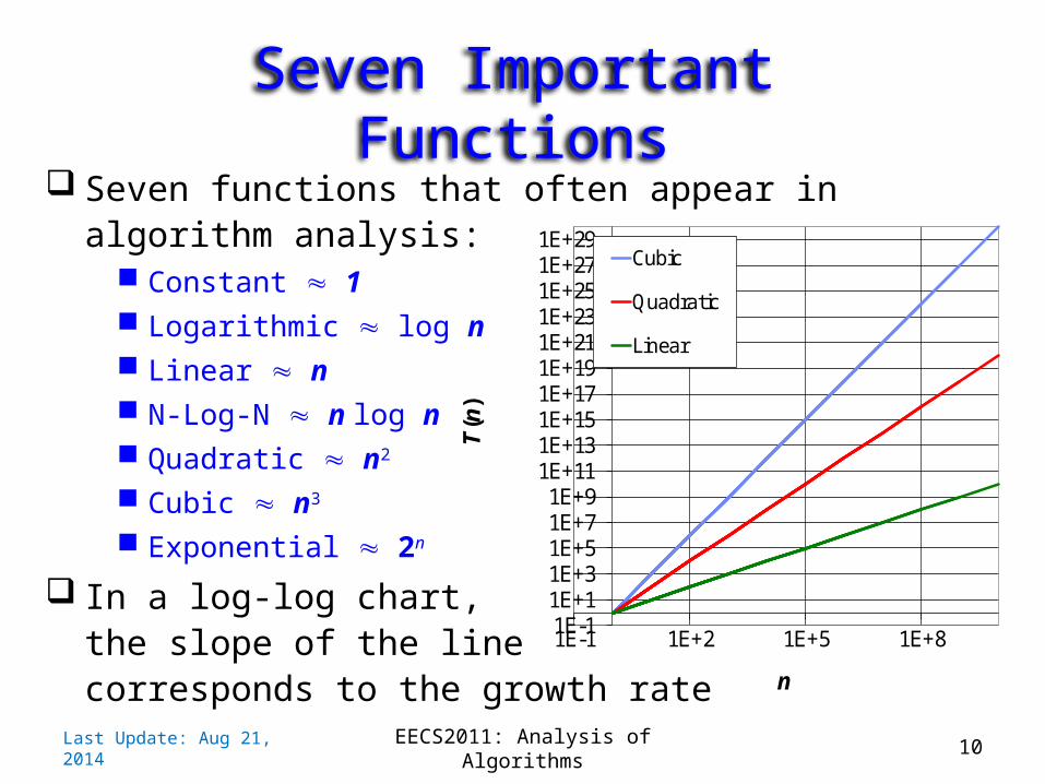
Seven Important Functions Seven functions that often appear in algorithm analysis:

Constant 1 Logarithmic log n Linear n N-Log-N n log n Quadratic n2

Cubic n3

Exponential 2n

In a log-log chart, the slope of the line corresponds to the growth rate



10

1E-11E+11E+31E+51E+71E+9

1E+111E+131E+151E+171E+191E+211E+231E+251E+271E+29

1E-1 1E+2 1E+5 1E+8

T(n

)

n

Cubic

Quadratic

Linear

Primitive Operations• Basic computations performed

by an algorithm• Identifiable in pseudocode• Largely independent from the

programming language• Exact definition not important

(we will see why later)• Assumed to take a constant

amount of time in the RAM model

Examples:– Evaluating an expression– Assigning a value to a

variable– Indexing into an array– Calling a method– Returning from a method



11

Counting Primitive OperationsBy inspecting the pseudocode, we can determine the maximum number of primitive operations executed by an algorithm, as a function of the input size



12

STEP 3 4 5 6 7 8 TOTAL

# ops 2 2 1+2n 2n 0 to 2n 1 4n+6 to 6n+6

Estimating Running Time• Algorithm arrayMax executes 6n + 6 primitive

operations in the worst case, 4n + 6 in the best case. Define:

a = Time taken by the fastest primitive operationb = Time taken by the slowest primitive operation

• Let T(n) be worst-case time of arrayMax. Thena (4n + 6) T(n) b(6n + 6)

• Hence, the running time T(n) is bounded by two linear functions



13

Growth Rate of Running Time• Changing the hardware/ software environment

o Affects T(n) by a constant factor, buto Does not alter the growth rate of T(n)

• The linear growth rate of the running time T(n) is an intrinsic property of algorithm arrayMax



14

Why Growth Rate Matters



15

if runtime is... time for n + 1 time for 2 n time for 4 n

c lg n c lg (n + 1) c (lg n + 1) c(lg n + 2)

c n c (n + 1) 2c n 4c n

c n lg n~ c n lg n

+ c n2c n lg n +

2cn4c n lg n +

4cn

c n2 ~ c n2 + 2c n 4c n2 16c n2

c n3 ~ c n3 + 3c n2 8c n3 64c n3

c 2n c 2 n+1 c 2 2n c 2 4n

runtimequadrupleswhen problemsize doubles

Comparison of Two Algorithms



16

insertion sort is n2 / 4

merge sort is 2 n lg n

sort a million items?insertion sort takes

roughly 70 hourswhile

merge sort takesroughly 40 seconds

This is a slow machine, but if100 x as fast, then it’s 40 minutesversus less than 0.5 seconds

Constant Factors• The growth rate is not

affected byo constant factors or o lower-order terms

• Exampleso 102n + 105

is a linear functiono 105n2 + 108n

is a quadratic function



17

1E-11E+11E+31E+51E+71E+9

1E+111E+131E+151E+171E+191E+211E+231E+25

1E-1 1E+2 1E+5 1E+8

T(n

)

n

Quadratic

Quadratic

Linear

Linear

Big-Oh Notation• Given functions f(n) and

g(n), we say that f(n) is O(g(n)) if there are positive constantsc and n0 such that

f(n) cg(n) for n n0

• Example: 2n + 10 is O(n)o 2n + 10 cno (c 2) n 10o n 10/(c 2)o Pick c = 3 and n0 = 10



18

1

10

100

1,000

10,000

1 10 100 1,000n

3n

2n+10

n

Big-Oh Example• Example:

the function n2 is not O(n)o n2 cno n co The above inequality cannot

be satisfied for all sufficiently large n, since c must be a constant



19

1

10

100

1,000

10,000

100,000

1,000,000

1 10 100 1,000n

n^2

100n

10n

n



20

More Big-Oh Examples 7n - 2

7n-2 is O(n)need c > 0 and n0 1 such that 7 n - 2 c n for n n0

this is true for c = 7 and n0 = 1

3 n3 + 20 n2 + 53 n3 + 20 n2 + 5 is O(n3)need c > 0 and n0 1 such that 3 n3 + 20 n2 + 5 c n3 for n n0


3 log n + 53 log n + 5 is O(log n)need c > 0 and n0 1 such that 3 log n + 5 c log n for n n0


Big-Oh and Growth Rate• The big-Oh notation gives an upper bound on the

growth rate of a function

• The statement “f(n) is O(g(n))” means that the growth rate of f(n) is no more than the growth rate of g(n)

• We can use the big-Oh notation to rank functions according to their growth rate



21

Big-Oh Rules• If f(n) is a polynomial of degree d,

then f(n) is O(nd), i.e.,o drop lower-order termso drop constant factors

• Use the smallest possible class of functionso Say “2n is O(n)” instead of “2n is O(n2)”

• Use the simplest expression of the classo Say “3n + 5 is O(n)” instead of “3n + 5 is O(3n)”



22

Asymptotic Algorithm Analysis• The asymptotic analysis of an algorithm

determines the running time in big-Oh notation• To perform the asymptotic analysis

o We find the worst-case number of primitive operations executed as a function of the input size

o We express this function with big-Oh notation• Example:

o We say that algorithm arrayMax “runs in O(n) time”• Since constant factors and lower-order terms are

eventually dropped anyhow, we can disregard them when counting primitive operations



23

Computing Prefix Averages• We further illustrate

asymptotic analysis with two algorithms for prefix averages

• The i-th prefix average of an array X is average of the first (i + 1) elements of X:A[i] = (X[0] + X[1] + … + X[i])/(i+1)

• Computing the array A of prefix averages of another array X has applications to financial analysis



24

0

5

10

15

20

25

30

35

1 2 3 4 5 6 7

X

A



25

Prefix Averages (Quadratic)The following algorithm computes prefix averages in quadratic time by applying the definition

Arithmetic Progression• The running time of

prefixAverage1 isO(1 + 2 + …+ n)

• The sum of the first n integers is n(n + 1) / 2– There is a simple visual

proof of this fact

• Thus, algorithm prefixAverage1 runs in O(n2) time



26

0

1

2

3

4

5

6

7

1 2 3 4 5 6



27

Prefix Averages 2 (Linear)The following algorithm uses a running sum to improve efficiency

Algorithm prefixAverage2 runs in O(n) time!

Math you need to Review• Properties of powers:

• Properties of logarithms:

• Summations

• Powers

• Logarithms

• Proof techniques

– Induction

– . . .

• Basic probability



28



29

Relatives of Big-Ohbig-Omega

f(n) is (g(n)) if there is a constant c > 0 and an integer constant n0 1 such that

f(n) c g(n) for n n0

big-Theta f(n) is (g(n)) if there are constants c’ > 0 and c’’ > 0

and an integer constant n0 1 such that

c’ g(n) f(n) c’’ g(n) for n n0

Intuition for Asymptotic Notation



30

big-Oh f(n) is O(g(n)) if f(n) is asymptotically less than or equal to g(n)

big-Omega f(n) is (g(n)) if f(n) is asymptotically greater than or equal to

g(n)

big-Theta f(n) is (g(n)) if f(n) is asymptotically equal to g(n)



31

Example Uses of the Relatives of Big-Oh

f(n) is (g(n)) if it is (n2) and O(n2). We have already seen the former, for the latter recall that f(n) is O(g(n)) if there is a constant c > 0 and an integer constant n0 1 such that f(n) < c g(n) for n n0 .

Let c = 5 and n0 = 1.

5n2 is (n2)

f(n) is (g(n)) if there is a constant c > 0 and an integer constant n0 1 such that f(n) c g(n) for n n0 .

Let c = 1 and n0 = 1.

5n2 is (n)

f(n) is (g(n)) if there is a constant c > 0 and an integer constant n0 1 such that f(n) c g(n) for n n0 .

Let c = 5 and n0 = 1.

5n2 is (n2)

Part 1: Summary• Analyzing running time of algorithms

o Experimentation & its limitationso Theoretical analysis

• Pseudo-code• RAM: Random Access Machine• 7 important functions• Asymptotic notations: O(), () , ()• Asymptotic running time analysis of algorithms



32



33

Part 2: Correctness


EECS2011: Analysis of Algorithms 34

Outline• Iterative Algorithms:

Assertions and Proofs of Correctness

• Binary Search: A Case Study



Assertions• An assertion is a statement about the state of the data

at a specified point in your algorithm.

• An assertion is not a task for the algorithm to perform.

• You may think of it as a comment that is added for the benefit of the reader.



Loop Invariants• Binary search can be implemented as an iterative

algorithm (it could also be done recursively).

• Loop Invariant: An assertion about the current state useful for designing, analyzing and proving the correctness of iterative algorithms.



Other Examples of Assertions• Pre-conditions: Any assumptions that must

be true about the input instance.• Post-conditions: The statement of what

must be true when the algorithm/program returns.

• Exit-condition: The statement of what must be true to exit a loop.



Iterative AlgorithmsTake one step at a time

towards the final destination

loop { if (done) { exit loop }

take step

}



From Pre-Condition to Post-Condition



Loop Invariant

Pre-Condition Post-Condition

Pre-Loop

Loop

Post-Loop

Establishing Loop Invariant



1. from the pre-condition on the input instance, establish the loop invariant.

1

Maintain Loop Invariant• Suppose that

1) We start in a safe location (loop invariant just established from pre-condition)

2) If we are in a safe location (loop invariant), we always step to another safe location (loop invariant)

• Can we be assured that the computation will always keep us in a safe location?

• By what principle?



2

Maintain Loop Invariant By Induction the computation will always be in a safe location.

loop invariant at the end of iteration (beginning of iteration )



1

2

Ending The Algorithm• Define Exit Condition

• Termination: With sufficient progress, the exit condition will be met.

• When we exit, we knowo loop invariant is trueo exit condition is true

3) from these we must establish the post-condition.



3

45

Iterative Algorithm



2

1

3Pre-loop

Loop-Invariant

Loop Body

Post-ConditionPre-Condition

YES

NO

Exit-Condition

Post-loop

Definition of Correctness<PreCond> & <code> <PostCond>

If the input meets the pre-conditions, then the output must meet the post-conditions.

If the input does not meet the preconditions, then nothing is required.



Binary Search:a case study



Define Problem: Binary Search• PreConditions

– Key 25– Sorted indexed List A

• PostConditions– Find key in list (if there).

3 5 6 13 18 21 21 25 36 43 49 51 53 60 72 74 83 88 91 95

3 5 6 13 18 21 21 25 36 43 49 51 53 60 72 74 83 88 91 95



Define Loop Invariant• Maintain a sub-list.• LI: If the key is contained in the original list,

then the key is contained in the sub-list.

key 25

3 5 6 13 18 21 21 25 36 43 49 51 53 60 72 74 83 88 91 95



Define Step• Cut sub-list in half.• Determine which half the key would be in.• Keep that half.

key 25

3 5 6 13 18 21 21 25 36 43 49 51 53 60 72 74 83 88 91 95

If key ≤ A[mid],then key is inleft half.

If key > A[mid],then key is inright half.

mid



Define Step• It is faster not to check if the middle element

is the key.• Simply continue.

key 43

3 5 6 13 18 21 21 25 36 43 49 51 53 60 72 74 83 88 91 95





Make Progress• The size of the list becomes smaller.

3 5 6 13 18 21 21 25 36 43 49 51 53 60 72 74 83 88 91 95

3 5 6 13 18 21 21 25 36 43 49 51 53 60 72 74 83 88 91 95



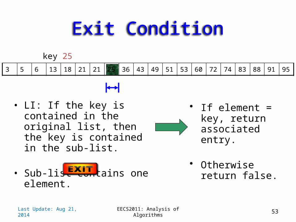
Exit Condition• LI: If the key is contained in the

original list, then the key is contained in the sub-list.

• Sub-list contains one element.

3 5 6 13 18 21 21 25 36 43 49 51 53 60 72 74 83 88 91 95

• If element = key, return associated entry.

• Otherwise return false.

key 25



Running Time The sub-list is of size

Each step O(1) time.Total time = O(log n)

key 25

3 5 6 13 18 21 21 25 36 43 49 51 53 60 72 74 83 88 91 95







Algorithm BinarySearch ( A[1..n] , key)<precondition>: A[1..n] is sorted in non-decreasing

order<postcondition>: If key is in A[1..n], output is its

locationp 1 , q n while p < q do

<Loop-invariant>: if key is in A[1..n], then key is in A[p..q]mid if key A[mid] then q mid

else p mid + 1 end whileif key = A[p]

then return (p)else return (“key not in list”)

end algorithm

Simple, right?• Although the concept is simple, binary search is

notoriously easy to get wrong.• Why is this?



Boundary Conditions• The basic idea behind binary search is easy to grasp.

• It is then easy to write pseudo-code that works for a ‘typical’ case.

• Unfortunately, it is equally easy to write pseudo-code that fails on the boundary conditions.



Boundary Conditionsor

What condition will break the loop invariant?



if key A[mid] then q midelse p mid + 1

if key < A[mid] then q midelse p mid + 1

Boundary Conditions

key 36

3 5 6 13 18 21 21 25 36 43 49 51 53 60 72 74 83 88 91 95

mid

sC eod lek cey t A[m rige hid] t lf: ha

Bug!!



Boundary ConditionsOK OK Not OK !!



if key A[mid] then q midelse p mid + 1

if key < A[mid] then q mid - 1else p mid

if key < A[mid] then q midelse p mid + 1

key 25

3 5 6 13 18 21 21 25 36 43 49 51 53 60 72 74 83 88 91 95

Boundary Conditionsmid

2

p q

mid 2

p q

or

Shouldn’t matter, right? Select mid 2

p q



6 74

Boundary Conditions

key 25

9591888372605351494336252121181353



mid



Select mid 2

p q

2518 74

Boundary Conditions

key 25

9591888372605351494336212113653



mid



Select mid 2

p q

2513 74

Boundary Conditions

key 25

9591888372605351494336212118653



Another bug!

No progress toward goal: Loops Forever!

midSelect mid

2p q



Boundary Conditions

OK OK Not OK !!



mid if key A[mid]

then q midelse p mid +

1

mid if key < A[mid]

then q mid - 1

else p mid

mid if key A[mid]


1

Getting it Right• How many possible algorithms?• How many correct algorithms?



mid if key A[mid]


1 then q mid -

1else p mid

or ?

mid or ?

if key < A[mid]

or ?

Alternative Algorithm: Less Efficient but More Clear



Algorithm BinarySearch ( A[1..n] , key)<precondition>: A[1..n] is sorted in non-decreasing

order<postcondition>: If key is in A[1..n], output is its locationp 1 , q n while p < q do

<Loop-invariant>: if key is in A[1..n], then key is in A[p..q]mid if key < A[mid]

then q mid - 1else if key > A[mid]

then p mid + 1 else return (mid)end whilereturn (“key not in list”)

end algorithm

Still O(log n), but with slightly larger constant.

Part 2: SummaryFrom Part 2, you should be able to:

Use the loop invariant method to think about iterative algorithms. Prove that the loop invariant is established. Prove that the loop invariant is maintained in the ‘typical’ case. Prove that the loop invariant is maintained at all boundary conditions. Prove that progress is made in the ‘typical’ case Prove that progress is guaranteed even near termination, so that the

exit condition is always reached. Prove that the loop invariant, when combined with the exit condition,

produces the post-condition.





69

Analysis of Algorithms Algorithm Input Output Last Update: Aug 21, 2014 EECS2011: Analysis of...

Documents

Transcript of Analysis of Algorithms Algorithm Input Output Last Update: Aug 21, 2014 EECS2011: Analysis of...