Analysis of Adaptive Mesh Refinement for IMEX Discontinuous GalerkinSolutions of the Compressible Euler Equations with Application to

Atmospheric Simulations

Michal A. Koperaa,∗, Francis X. Giraldoa

aNaval Postgraduate School, Department of Applied Mathematics, Monterey, CA 93940

Abstract

The resolutions of interests in atmospheric simulations require prohibitively large computational resources.Adaptive mesh refinement (AMR) tries to mitigate this problem by putting high resolution in crucial areas ofthe domain. We investigate the performance of a tree-based AMR algorithm for the high order discontinuousGalerkin method on quadrilateral grids with non-conforming elements. We perform a detailed analysis ofthe cost of AMR by comparing this to uniform reference simulations of two standard atmospheric testcases: density current and rising thermal bubble. The analysis shows up to 15 times speed-up of the AMRsimulations with the cost of mesh adaptation below 1% of the total runtime. We pay particular attention tothe implicit-explicit (IMEX) time integration methods and show that the ARK2 method is more robust withrespect to dynamically adapting meshes than BDF2. Preliminary analysis of preconditioning reveals that itcan be an important factor in the AMR overhead. The compiler optimizations provide significant runtimereduction and positively affect the effectiveness of AMR allowing for speed-ups greater than it would followfrom the simple performance model.

Keywords: adaptive mesh refinement, discontinuous Galerkin method, non-conforming mesh, IMEX,compressible Euler equations, atmospheric simulations

1. Introduction

Atmospheric flows are characterized by a vast spectrum of spatial and temporal scales, from weatherfronts and planetary waves covering thousands of kilometers and lasting weeks, to turbulent motions atthe micro scale. Due to limitations in computational resources, we are not able to resolve all phenomena.Most models assume a uniform mesh and therefore distribute computational resources uniformly across thedomain. The scales of motion in the atmosphere are not, however, distributed uniformly both in space andtime. The goal of adaptive mesh refinement (AMR) is to focus the resolution of the mesh (and thereforecomputational resources) where it is most required. Dynamic adaptation aims to follow the importantstructures of the flow and modify the mesh as the simulation progresses, according to some refinementcriterion. An example of such a situation in the atmosphere is a hurricane, which is an event of significancethat is relatively localized within a global domain but traverses vast distances. Static adaptation, on theother hand, aims to refine the mesh once at the beginning of the simulation, which allows to focus thecomputational resources at a particular area of interest in the domain. In such a way one could well resolvea certain part of the globe for which the weather forecast is to be performed, leaving the rest of the domainat much coarser resolution. In this paper we focus on dynamic mesh refinement, which we present on acouple of atmospheric test cases. All the methods that we discuss, however, are readily applicable to staticadaptation.

∗Corresponding author. Tel: +1 831-656-3247Email addresses: makopera@nps.edu (Michal A. Kopera ), fxgirald@nps.edu (Francis X. Giraldo)

In order to discretize the solution we use the discontinuous Galerkin (DG) method on quadrilateralelement grids. The DG method has gained a significant level of interest in recent years and there has beena number of efforts to apply it to hydrostatic [1] and nonhydrostatic [2] atmospheric flows. The methodbenefits from great data locality and high computation intensity, which helps to scale exceptionally well ona large number of processors. It also supports arbitrary high order, which, among other benefits, allows foraccurate handling of the non-conforming edge fluxes, which can arise in the process of mesh adaptation.AMR for DG was successfully applied in different applications (e.g. shock capturing [3, 4], mantle convection[5]). Here we focus on atmospheric flows, particularly the dry dynamics governed by the Euler equation.

The question we would like to answer is: how does AMR benefit a simulation? To try to answer thisquestion we perform a detailed analysis of the cost of AMR comparing this to the results of a uniformlyrefined simulation. To our knowledge, such a detailed study has not been performed previously. Moreover,we seek to answer this question in light of the use of implicit-explicit (IMEX) time-integrators because forreal-world applications (such as weather and climate modeling) explicit time-integration is not feasible dueto the small time-step restriction of the fast acoustic waves.

The following subsections present a brief overview of the work done on AMR for atmospheric simulationin general and specifically in conjunction with the DG method.

1.1. AMR in atmospheric simulations

Jablonowski [6] and Behrens [7] give a good overview of the state of adaptive atmospheric modeling.The hurricane modeling community was the first to use nested grid techniques for their simulations. In thisapproach fine scale grids were nested into large-scale coarse meshes and communication was allowed fromlarge to small scales [8, 9] or in both directions [10]. The nested grid can move with the feature it tracks, butoften some previous knowledge of the grid movement is required and the number of points remains constantthroughout the simulation.

Another example of a mesh modification technique which preserves the number of points and grid con-nectivity throughout the simulation is mesh stretching, i.e., changing the grid spacing by the use of trans-formation functions (also known as r-refinement). Examples of such an approach are presented in [11, 12]and more recently in [13].

This paper focuses on an adaptive method which does not involve a moving mesh but rather refines theelements dynamically in regions of particular interest. This technique is typically referred to as dynamicAMR. The first atmospheric models involving AMR were developed by Skamarock and Klemp [14, 15].They used the technique of Berger and Oliger [16] where a finite difference method is used to integrate thedynamical equations first on a coarse and then on the finer grids. In order to determine the location of finergrids a criterion based on truncation error estimation was used. The technique of Berger and Oliger [16]and Berger and Collela [17] is referred to as block-structured AMR. It was later used in a number of studiesincluding LeVeque [18] and Nikiforakis [19].

The only operational weather model which uses dynamic AMR is OMEGA [20]. OMEGA is based onthe finite volume MPDATA scheme, originally developed by Smolarkiewicz [21], which uses unstructuredtriangular meshes. The dynamic adaptation capabilities were implemented to the MPDATA model by Iselinand coworkers [22]. Another example of AMR which uses triangular elements is the work of Giraldo [23]who used the Lagrange-Galerkin method. In all of these approaches the mesh is obtained by a Delaunaytriangulation of the domain given some mesh size criteria. When the criterion indicates that the mesh shouldbe adjusted, the triangulation is performed on the entire domain, and the solution is projected from the oldmesh to the new one.

A different approach is presented in the work of Behrens [24, 25], where the triangular elements indicatedfor refinement are subdivided making sure the conformity of the edges is preserved. The method allows forlocal refinement without modifying the entire domain. It is well suited for triangular meshes, however thesame approach for quadrilateral grids would be difficult as maintaining conformity of locally dynamicallyrefined quadrilaterals is more challenging to achieve. An example of static conforming quadrilateral meshrefinement can be found in [26].

Quadrilateral meshes yield to local refinement easily, provided that we allow non-conforming elementsin the grid. Examples of quadrilateral-based dynamic AMR methods for the shallow water equations can

2

be found in the work of Jablonowski [6]. St-Cyr et al. [27] compare an adaptive cubed-sphere grid spectralelement shallow water model with an adaptive finite volume method by [6] to investigate the applicabilityof tree-based AMR algorithms to atmospheric models.

1.2. Element based Galerkin methods for atmospheric AMR

The high order element based Galerkin methods for AMR in atmospheric applications is a fairly new fieldof study. These methods present a new set of challenges and possibilities for adaptive mesh refinement. Byexpanding the solution in a basis of high order polynomials in each element, one can dynamically adjust theorder of these basis functions, which can differ across elements. This kind of approach is called p-refinement,and an example of such a technique applied to the shallow water equations can be found in [28].

In the previous section we already mentioned the element mesh refinement (so called h-refinement),which focuses on refining the mesh while keeping the polynomial order constant across the elements. If wechoose to allow non-conforming elements, the challenge in this approach is the appropriate treatment of thenon-confoming faces. For the DG method one needs to compute the flux across the non-conforming faces.The mathematical solution to this problem was proposed by Kopriva [29] as well as Maday et al. [30] whoformulated the mortar method for non-conforming elements. Examples of application of h-refinement toatmospheric flows can be found in [31], where the spectral element method for geophysical and astrophysicalapplications was used, or [27] where the comparison of a finite volume and spectral element AMR code forthe shallow water equations was performed. A recent study by Muller et al. [32] investigates the dynamicadaptation of triangular conforming meshes and addresses the question whether coarsening the mesh incertain areas of the grid affects the solution in a significant way. Brdar et al. [33] perform the comparisonof two dynamical cores for the numerical weather prediction and mention that the DUNE code, which usesthe DG method, has AMR capabilities, however no adaptive mesh examples are discussed in that paper.

The p and h refinement methods can be combined together. [34] shows the application of such analgorithm for the DG method using triangular, non-conforming elements applied to shallow water equa-tions. Another example for this set of equations is presented in [35], where an hp-adaptive DG method onquadrilateral, non-conforming elements for global tsunami simulations is considered.

In this paper we focus on the quadrilateral, non-conforming DG method for the Euler equations andprovide an in-depth analysis of the performance of our implementation. To our knowledge this is the firstwork on tree-based non-conforming AMR for the nonhydrostatic atmosphere equations. Furthermore, toour knowledge no previous work has been published on non-conforming AMR for high-order DG methodsfor these equations.

This paper is organized as follows: section 2 gives a brief overview of the equations we are solving, section3 provides an outline of the DG method, section 4 discusses the difference between conforming and non-conforming mesh. In section 5 we describe the details of the mesh adaptation algorithm. Finally, in section7 we provide the outline of the test cases followed by the discussion of the results in section 8. The paperis concluded in section9 and supplemented with an Appendix, which describes in detail the formulation ofthe projection method.

2. Governing equations

Non-hydrostatic atmospheric dynamical processes in NUMA1 are governed by the compressible Eulerequations in conservative form which uses density ρ, momentum ρu and density potential temperature ρθas state variables (see, e.g., [36] for other forms). We use the following equation set:

∂ρ

∂t+∇ · (ρu) = 0,

∂ρu

∂t+∇ · (ρu⊗ u + P I) = −ρgk +∇ · (µρ∇u), (1)

∂ρθ

∂t+∇ · (ρθu) = ∇ · (µρ∇θ),

1NUMA is the name of our model and is an acronym for the Nonhydrostatic Unified Model of the Atmosphere

3

where u = (u,w)T is the velocity field, ∇ = ( ∂∂x ,

∂∂z )T is the gradient operator, ⊗ is the tensor product, I

is the rank-2 identity matrix, k = (0, 1)T is the directional vector that points along the z direction, g is thegravitational acceleration and P is the pressure obtained from the equation of state

P = P0

(Rρθ

P0

) cpcv

. (2)

The dynamical viscosity µ is varied among the test cases. Note that while this is not the mathematicallyproper form of the true Navier-Stokes viscous stresses, it is sufficient for the chosen test cases as shownin Giraldo and Restelli [36]. Additional terms requiring definition are the pressure at the lower boundaryP0 = 1 × 105 Pa, the gas constant R = cp − cv and the specific heats at constant pressure and volume, cpand cv.

3. Discontinuous Galerkin method

Giraldo and Restelli [36] describe in detail the discretisation of Eq. (1) for the DG method. Here weoutline the weak formulation for the sake of completeness. Note that for the sake of brevity the analysis inthis paper was conducted using the weak form only, although both strong and weak forms are implementedin the NUMA software with the non-conforming AMR algorithm.

To describe the DG method, we write Eq. (1) in vector form

∂q

∂t+∇ · F = S(q),

where q = (ρ,UT ,Θ)T is the solution vector with U = ρu and Θ = ρθ. F(q) is the flux tensor given by

F(q) =

UU⊗Uρ + P I−∇

(µρ∇U

ρ

)θU− µ∇Θ

, (3)

and the source term S(q) given by

S(q) =

0−ρgk

0

. (4)

We divide the computational domain Ω into a set of non-overlapping elements Ωe such that Ω =Ne⋃e=1

Ωe.

We define the reference element I = [−1, 1]2 and for each element Ωe there exists a smooth transformationsuch that I = FΩe

(Ωe). Additionally, if Ωe = Ωe(x, y) and I = I(ξ, η) then FΩe: (x, y) → (ξ, η) and

F−1Ωe

: (ξ, η)→ (x, y). We employ the notation x = (x, y) and ξ = (ξ, η). The Jacobian of this transformation

is given by JΩe=

dFΩe

dξ with determinant JΩe.

Let ψk be a basis function of a space PN (I) of polynomials of degree N or lower in I where the index kvaries from 1 to K = (N + 1)2. The tensor product structure of I allows us to construct such a basis as

ψk = hi(ξ)hj(η),

where hiNi=0 is a basis for PN ([−1, 1]) and index k is uniquely associated with the pair (i, j): k = (i+ 1) +(N + 1)j. Let ξi be the Legendre-Gauss-Lobatto (LGL) points defined as the roots of (1 − ξ2)P ′N (ξ) = 0,where PN (ξ) is the N th order Legendre polynomial. The basis functions hi(ξ) are in fact the Lagrangepolynomials associated with LGL points ξi. Notice that associated with these points are the Gaussianquadrature weights

ωi =2

N(N + 1)

(1

PN (ξi)

)2

.

4

Let qN be the approximation of the solution vector q on the element Ωe in the expansion basis ψ:

qN (x, t)|Ωe=

K∑k=1

ψk(F−1

Ωe(x))qk(t), e = 1, . . . , Ne, (5)

where we introduce the grid points xk = FΩe( (ξi, ηj) ) and the grid point values qk(t) = qN (xk, t). The

computation of the derivatives of qN gives

∂qN∂x

(x, t)

∣∣∣∣Ωe

=

K∑k=1

d

dx

[ψk(F−1

Ωe(x)) ]

qk(t), (6)

∂qN∂t

(x, t)

∣∣∣∣Ωe

=

K∑k=1

ψk(F−1

Ωe(x)) dqkdt

(t). (7)

Concerning the computations of integrals, the expansion defined by Eq. (5) yields∫Ωe

qN (x, t) dx =

∫I

qN (x (ξ) , t) JΩe(ξ) dξ '

N∑i,j=0

ωiωj qkij (t)JΩe(ξi, ηj). (8)

With the definitions of the solution expansion and the operations of differentiation and integration inplace we can now formulate a DG representation of Eq. (1). Here we consider a nodal formulation withinexact integration as described in [36]. We start with multiplying Eq. (1) by a test function ψ and integratingover an element Ωe: ∫

Ωe

ψ

(∂qeN∂t

+∇ · F(qeN )

)dΩ =

∫Ωe

ψ S(qeN ) dΩe, (9)

where qeN denotes the degrees of freedom collocated in Ωe. Applying now integration by parts and intro-ducing the numerical flux F∗, the following problem is obtained:find qN (·, t) ∈ V DGN such that ∀Ωe, e = 1, . . . , Ne∫

Ωe

ψ∂qeN∂t

dΩe +

∫Γe

ψ n · F∗(qN ) dΓe −∫

Ωe

∇ψ · F(qeN ) dΩe =

∫Ωe

ψ S(qeN ) dΩ, (10)

∀ψ ∈ L2(Ω) .The coupling between neighboring elements is then recovered through the numerical flux F ∗, which is

required to be a single valued function on the interelement boundaries and the precise definition of which isgiven in [36].

By virtue of Eqs. (6), (7) and (8), Eq. (10) can be written in the matrix form

dqe

dt+(M

s,e)TF ∗(q)−

(De)TF (qe) = S(qe) (11)

where Ms,e

= (Me)−1M s,e and D

e= (Me)

−1De. Me, M s,e and De are local mass, boundary mass and

differentiation matrices given by

Mehk = wh|JΩe

(ξh) |δhk, Dehk = wh|JΩe

(ξh) |∇φk(xh), M s,ehk = wsh|JsΩe

(ξh) |δhk n(xh),

where h, k = 1, . . . ,K, δhk is the Kronecker delta, ξk = (ξi, ηj), wk = ωiωj , wsk = ωi for j = 0 or j = N and

wsk = ωj for i = 0 or i = N .Note that this equation can be simplified to yield the following semi-discrete weak form

dqeidt

=(De

ij

)TF ej + Sei −

ws,ei |Js,ei |

wei |Jei |(ns,ei )

TF ∗i . (12)

In Eq. (10) we notice that there is only one integral (Γe) which couples the neighboring elements together.It is this boundary integral that needs to be modified in order to handle non-conforming AMR. This isexplained in detail in Sec. 6.

5

4. Conforming vs non-conforming mesh

The first question that needs to be answered when constructing the AMR algorithm is whether non-conforming elements are allowed in the grid - that is whether each edge can be shared by more than twoelements. We can restrict ourselves to purely conforming ones, where all edges in the mesh are owned bytwo elements only. In the conforming case, the entire burden of handling the changing mesh falls on themesh adaptation algorithm, which has to make sure that the grid remains conforming after adaptation.The upside of this approach is an easy communication between neighboring elements. Since their edges areconforming, the AMR does not introduce any additional complication to the DG method solver.

In contrast, in the non-conforming case the mesh adaptation algorithm is kept simple: we divide eachelement marked for adaptation into a predefined number of children elements. In our case, we choose todivide a 2D quadrilateral element into four children elements (from here on, we shall refer to quadrilateralsas quads). This leads to a situation where, if only one of two neighbor elements is refined, the non-refinedneighbor shares an edge with two children elements. This requires the DG solver to be able to compute thenumerical flux on such a non-conforming edge. This approach shifts the burden from the mesh adaptationalgorithm to the solver side.

In this paper we present the non-conforming approach for a 2D quad-based mesh for the DG method2. We believe that the added complication and increased cost related to the computation of fluxes throughnon-conforming edges is more than made up for by the simplified element refinement algorithm.

5. Mesh adaptation algorithm

5.1. Forest of quad-trees

We adopt the forest of quad-trees approach proposed by [37]. We generate an initial coarse mesh, whichhas to represent the geometrical features of the domain. In Fig. 1a we present a simple two element initialmesh. We call it the level 0 mesh, where each element is a root for a tree of children elements. If wedecide to refine element 1, we replace this element with four children, which belong to the level 1 mesh. Werepresent it graphically on the right panel of Fig. 1b. Active elements (a set of elements which pave thedomain entirely) are marked in blue. Element number 1 is now inactive, replaced by the four newly createdelements 3, 4, 5 and 6.

If we further choose to refine element number 5, and thus introduce level 2 elements, we render thiselement inactive and replace it with the four children 7, 8, 9 and 10. Our element tree is presented in Fig.1c. Now elements 1 and 5 are no longer active while the active elements 2, 3, 4, 6, 7, 8, 9 and 10 form ourmesh.

5.2. Space filling curve

In the previous subsection’s examples we assigned numbers to the elements. Those numbers serve aselement unique labels. In order to traverse all active elements in the mesh, we utilize the concept of thespace filling curve (SFC). To each active element we assign an index, which defines the element’s positionin the space filling array. In order to index all the active elements in the mesh, we search each quad-tree inthe forest for active elements (leaves) starting with the first root element (element 1). Since it is inactive,we move to its first child. If the child element is active, we include it into the space filling curve and moveto the next child; if it is inactive we recursively traverse the sub-tree rooted in this element. After finishingthe search of one quad-tree, we move to the next level 0 root element.

Figure 2 illustrates the space filling curve concept. Note that the same tree traversing technique canyield different space filling curves, depending on the numbering of children elements. The numbering thatproduced the curve in Fig. 2a imposes a row-major order of children elements, while the curve in Fig. 2bwas generated using counter-clockwise enumeration. The numbering is applied recursively, starting from the

2It should be noted that doing this for the continuous Galerkin method is also possible but slightly more complicated. Weshall report on this in a follow-up paper.

6

Figure 1: Unstructured grid organized into a forest of quad-trees.

level 0 mesh and traversing the tree to its fullest depth. Therefore in the row-major order we first numberthe elements of the level 0 mesh as (1, 2). Next we move one level down and enumerate the children ofelement 1 (element 2 has no children) starting from the bottom left element and enumerating the children inthe bottom row first, then move to the second row and enumerate the remaining two elements. We repeatthe recursive procedure until we enumerate all the elements on all levels.

In DG methods we prefer indexing the elements in such a way that adjacent elements are placed closeto each other in the space filling curve. This increases data locality, which in turn makes the computationof fluxes more efficient. Data locality is particularly important in parallel implementations of the AMRalgorithm, however a full study of the influence of element numbering on the efficiency of the code exceedsthe scope of this paper.

5.3. Element division technique

To keep the adaptation algorithm simple, and the non-conforming face handling as efficient as possible(see Section 6.1), we require that each side of an element to be refined is divided in a 2:1 size ratio. This meansthat we split a parent edge into two children edges of equal length. In NUMA we use general quadrilaterals,possibly with curved edges, which could prove splitting elements in physical (x, y) space difficult. Thereforewe perform the element splitting in the computational space (ξ, η) instead (see Fig. 3a).

In Section 3 we defined the transformation F : (x, y)→ (ξ, η). The inverse mapping F−1 : (ξ, η)→ (x, y)is simply the expansion of a variable in the polynomial basis ψ:

q(xj , yj) =

K∑i=1

qiψi(ξj , ηj),

where q is a variable defined in physical space, qi is the nodal value of the variable in computational spaceat node i corresponding to a basis function ψi. (ξj , ηj) represent coordinates of the j-th nodal point incomputational space, which corresponds to a point (xj , yj) in physical space.

We can treat the x and y coordinates of the nodal points as a variable across the element, which yields

7

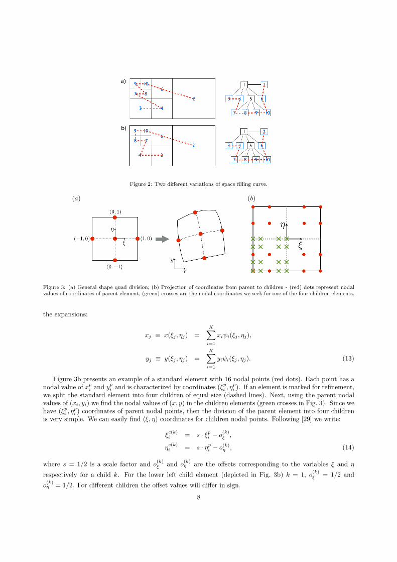
Figure 2: Two different variations of space filling curve.

(a) (b)

Figure 3: (a) General shape quad division; (b) Projection of coordinates from parent to children - (red) dots represent nodalvalues of coordinates of parent element, (green) crosses are the nodal coordinates we seek for one of the four children elements.

the expansions:

xj ≡ x(ξj , ηj) =

K∑i=1

xiψi(ξj , ηj),

yj ≡ y(ξj , ηj) =

K∑i=1

yiψi(ξj , ηj). (13)

Figure 3b presents an example of a standard element with 16 nodal points (red dots). Each point has anodal value of xpi and ypi and is characterized by coordinates (ξpi , η

pi ). If an element is marked for refinement,

we split the standard element into four children of equal size (dashed lines). Next, using the parent nodalvalues of (xi, yi) we find the nodal values of (x, y) in the children elements (green crosses in Fig. 3). Since wehave (ξpi , η

pi ) coordinates of parent nodal points, then the division of the parent element into four children

is very simple. We can easily find (ξ, η) coordinates for children nodal points. Following [29] we write:

ξc(k)i = s · ξpi − o

(k)ξ ,

ηc(k)i = s · ηpi − o

(k)η , (14)

where s = 1/2 is a scale factor and o(k)ξ and o

(k)η are the offsets corresponding to the variables ξ and η

respectively for a child k. For the lower left child element (depicted in Fig. 3b) k = 1, o(k)ξ = 1/2 and

o(k)η = 1/2. For different children the offset values will differ in sign.

8

(a) (b)

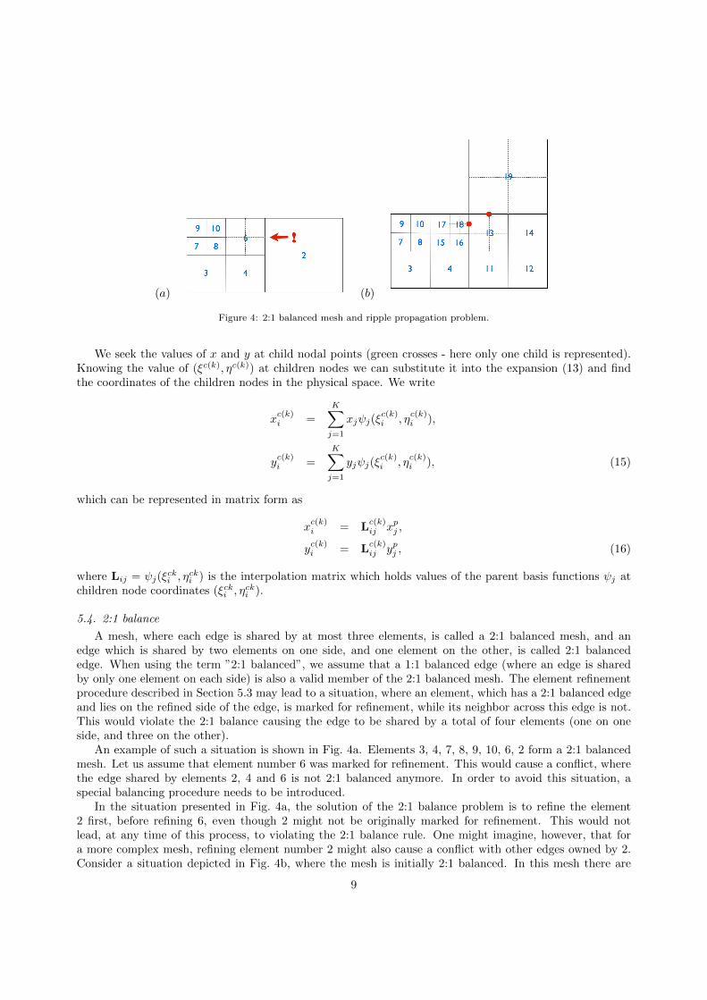
Figure 4: 2:1 balanced mesh and ripple propagation problem.

We seek the values of x and y at child nodal points (green crosses - here only one child is represented).Knowing the value of (ξc(k), ηc(k)) at children nodes we can substitute it into the expansion (13) and findthe coordinates of the children nodes in the physical space. We write

xc(k)i =

K∑j=1

xjψj(ξc(k)i , η

c(k)i ),

yc(k)i =

K∑j=1

yjψj(ξc(k)i , η

c(k)i ), (15)

which can be represented in matrix form as

xc(k)i = L

c(k)ij xpj ,

yc(k)i = L

c(k)ij ypj , (16)

where Lij = ψj(ξcki , η

cki ) is the interpolation matrix which holds values of the parent basis functions ψj at

children node coordinates (ξcki , ηcki ).

5.4. 2:1 balance

A mesh, where each edge is shared by at most three elements, is called a 2:1 balanced mesh, and anedge which is shared by two elements on one side, and one element on the other, is called 2:1 balancededge. When using the term ”2:1 balanced”, we assume that a 1:1 balanced edge (where an edge is sharedby only one element on each side) is also a valid member of the 2:1 balanced mesh. The element refinementprocedure described in Section 5.3 may lead to a situation, where an element, which has a 2:1 balanced edgeand lies on the refined side of the edge, is marked for refinement, while its neighbor across this edge is not.This would violate the 2:1 balance causing the edge to be shared by a total of four elements (one on oneside, and three on the other).

An example of such a situation is shown in Fig. 4a. Elements 3, 4, 7, 8, 9, 10, 6, 2 form a 2:1 balancedmesh. Let us assume that element number 6 was marked for refinement. This would cause a conflict, wherethe edge shared by elements 2, 4 and 6 is not 2:1 balanced anymore. In order to avoid this situation, aspecial balancing procedure needs to be introduced.

In the situation presented in Fig. 4a, the solution of the 2:1 balance problem is to refine the element2 first, before refining 6, even though 2 might not be originally marked for refinement. This would notlead, at any time of this process, to violating the 2:1 balance rule. One might imagine, however, that fora more complex mesh, refining element number 2 might also cause a conflict with other edges owned by 2.Consider a situation depicted in Fig. 4b, where the mesh is initially 2:1 balanced. In this mesh there are

9

two levels of refinement predefined. Element 19 is a 0th level element, elements 3, 4, 11, 12, 13, 14 are 1stlevel elements and 7-10 and 15-18 are 2nd level. Let us assume we want to refine element number 18, whichwould create 3rd level children elements. This would create a conflict with element 13, which is a 1st levelelement. Therefore we refine element number 13 to the 2nd level, but this creates a conflict with the 0th

level element number 19. In order to refine 18, we need to refine element 19 first, then 13, and finally 18in order to keep 2:1 balance at all times. This causes some regions of the domain to be more refined thanrequired from the refinement criterion - we did not initially intend to refine 13 or 19. Such phenomenon iscalled the ripple effect, where refinement of one element can cause an entire area not directly neighboringthe element in question to be refined [38].

It is easy to show that in the 2D case the ripple propagation is limited by the lowest level element inthe mesh. In a 2:1 balanced mesh the level difference between neighboring elements can be at most 1. Theconflict can occur only when refining an n-th level element which has a neighbor of level (n− 1). Thereforewe need to bring the (n− 1) level element to level n before refining the original element to level (n+ 1). Ifin turn the (n− 1) level element causes conflict with (n− 2) level element, we need to follow the balancingprocedure recursively. In the worst case scenario we will propagate the ripple down to 0th level element,which by definition is a root of the element tree. Therefore by refining one n-th level element we may beforced, in the worst case, to refine n other elements. This will cause 4n new elements to be created inthe areas possibly not indicated by the refinement criterion. 4n is typically a very small number since thesimulations shown in this work tend to have values n <= 5.

In the case of element coarsening, we adopt a different strategy. If coarsening of an element would causea conflict (consider a situation in Fig. 4b after refining all indicated elements, when we want to de-refineelement 19), we do not perform this operation. In order to keep the 2:1 balance we avoid propagating ade-refinement ripple to higher levels. The rationale behind this strategy is that it is better to have morerefined elements than we need, rather than lack the resolution in the areas where it is necessary. This waywe ensure that we always have the appropriate level of refinement as indicated by the refinement criterion.

5.5. Refinement criterion

Our focus in this paper is the AMR machinery and its particular application to the DG method, thereforewe use a very simple mesh refinement criterion. First, we specify the quantity of interest (QOI). It can beeither a primitive variable like θ, u, w or ρ, or an expression derived from those variables (i.e. velocitymagnitude, absolute value of temperature fluctuation etc.). We then choose a refinement threshold. If themaximum value of the QOI within an element falls below the threshold, the element is marked for refinement.The maximum criterion can be of course replaced by a minimum criterion. It is also worthwhile to considera gradient, or other derivatives of primitive variables, as a QOI. Throughout this paper we use the potentialtemperature perturbation as the quantity of interest.

The refinement criterion typically need not be evaluated every time-step, but rather every predefinednumber of steps, depending on the particular problem. After each evaluation of the criterion for all activeelements in the grid, the balancing algorithm is run to eliminate possible conflicts.

6. Handling of non-conforming edges

The previous section described the details of the mesh refinement algorithm. Here we will focus on theimplementation of such an algorithm to a DG solver. Sections 6.1 and 6.2 describe the computation of theflux for the DG method.

6.1. Projection onto 2:1 edges

In the DG method at every time-step we need to evaluate the numerical flux through all the elementedges. When allowing non-conforming elements in the mesh, one needs to address the problem of projectingthe data between two sides of a non-conforming edge. In our case the non-conformity is limited to 2:1balanced edges, which makes the data exchange slightly easier than in a general non-conforming case.

10

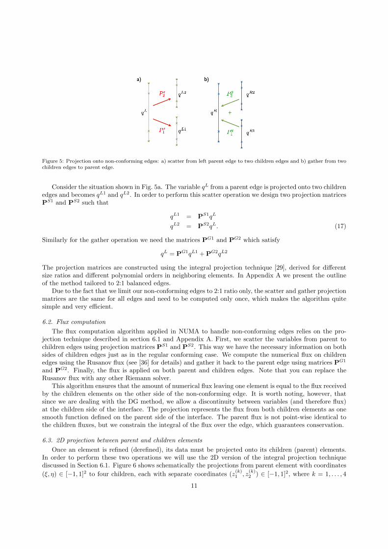
Figure 5: Projection onto non-conforming edges: a) scatter from left parent edge to two children edges and b) gather from twochildren edges to parent edge.

Consider the situation shown in Fig. 5a. The variable qL from a parent edge is projected onto two childrenedges and becomes qL1 and qL2. In order to perform this scatter operation we design two projection matricesPS1 and PS2 such that

qL1 = PS1qL

qL2 = PS2qL. (17)

Similarly for the gather operation we need the matrices PG1 and PG2 which satisfy

qL = PG1qL1 + PG2qL2

The projection matrices are constructed using the integral projection technique [29], derived for differentsize ratios and different polynomial orders in neighboring elements. In Appendix A we present the outlineof the method tailored to 2:1 balanced edges.

Due to the fact that we limit our non-conforming edges to 2:1 ratio only, the scatter and gather projectionmatrices are the same for all edges and need to be computed only once, which makes the algorithm quitesimple and very efficient.

6.2. Flux computation

The flux computation algorithm applied in NUMA to handle non-conforming edges relies on the pro-jection technique described in section 6.1 and Appendix A. First, we scatter the variables from parent tochildren edges using projection matrices PS1 and PS2. This way we have the necessary information on bothsides of children edges just as in the regular conforming case. We compute the numerical flux on childrenedges using the Rusanov flux (see [36] for details) and gather it back to the parent edge using matrices PG1

and PG2. Finally, the flux is applied on both parent and children edges. Note that you can replace theRusanov flux with any other Riemann solver.

This algorithm ensures that the amount of numerical flux leaving one element is equal to the flux receivedby the children elements on the other side of the non-conforming edge. It is worth noting, however, thatsince we are dealing with the DG method, we allow a discontinuity between variables (and therefore flux)at the children side of the interface. The projection represents the flux from both children elements as onesmooth function defined on the parent side of the interface. The parent flux is not point-wise identical tothe children fluxes, but we constrain the integral of the flux over the edge, which guarantees conservation.

6.3. 2D projection between parent and children elements

Once an element is refined (derefined), its data must be projected onto its children (parent) elements.In order to perform these two operations we will use the 2D version of the integral projection techniquediscussed in Section 6.1. Figure 6 shows schematically the projections from parent element with coordinates

(ξ, η) ∈ [−1, 1]2 to four children, each with separate coordinates (z(k)1 , z

(k)2 ) ∈ [−1, 1]2, where k = 1, . . . , 4

11

Figure 6: Projection between parent and children elements - 2D extension of integral projection for non-conforming edges.

enumerates the children elements. For this projection we construct the scatter matrix PSk2D . The inverseoperation is performed using the gather matrix PGk2D . Detailed construction of both matrices is described inAppendix A. Note that while the integral projection method works well for conserved quantities, it may notbe appropriate for all variables in the problem. It is sometimes better to interpolate or recompute certainquantities, if possible. An example of such a situation is the gravity direction vector, which is definedcompletely by the input to the simulation, therefore can be recomputed for each new element in the mesh.In both cases presented in this paper the gravity direction was k = (0, 1) and in some cases the projectionoperation caused inconsistencies on the order of the round-off error, which in turn adversely affected thesolution.

7. Test cases

In order to test the AMR algorithm we run a selection of cases from the set presented in [36]. The setconsists of seven tests widely used for benchmarking of non-hydrostatic dynamical cores of numerical weatherprediction codes. For the purpose of benchmarking the AMR capabilities of our code we have picked twoscenarios. The density current and rising thermal bubble cases show the performance of the AMR algorithmon a rapidly changing mesh. For both test cases we compare the adaptively refined simulation with auniformly refined simulation. Both cases are described in detail in the aforementioned paper. Here weoutline them for completeness.

7.1. Case 1: Density current

The case was first published in [39] and consists of a bubble of cold air dropped in a neutrally stratifiedatmosphere. The bubble eventually hits the lower boundary of the domain (no flux wall) and moves hori-zontally shedding Kelvin-Helmholtz rotors. In order to obtain the grid-converged solution we apply artificialviscosity µ = 75m2/s(see [39]).

The initial condition is defined in terms of potential temperature

θ′ =

0 for r > rcθc2

(1 + cos

(πrrc

))for r ≤ rc

, (18)

where θc = −15K, r =

√(x−xc

xr

)2

+(z−zczr

)2

and rc = 1. The domain is defined as (x, z) ∈ [0, 25600] ×[0, 6400] m with t ∈ [0, 900] s and the center of the bubble is at (xc, zc) = (0, 3000) m with the size of thebubble defined by (xr, zr) = (4000, 2000) m. The boundary conditions for all four boundaries are no-fluxwalls. The velocity field is initially set to zero everywhere.

12

(a)

(b)

(c)

(d)

Figure 7: Snapshots of the solution and dynamically adaptive mesh for θt = 1.0 at different simulation times: (a) 1s, (b) 300s,(c) 600s, and (d) 900s.

7.2. Case 2: Rising thermal bubble

In this test case a warm bubble rises in a constant potential temperature atmosphere (θ = 300K). As itrises, it deforms until it forms a mushroom shape. Initially, the air is at rest and in hydrostatic balance. Theinitial potential temperature perturbation is given by Eq. (18) with θc = 0.5K and rc = 250m. The domainhas dimensions (x, z) ∈ [0, 1000]m ×[0, 1000]m and the bubble is positioned at (xc, zc) = (500, 350)m. Theboundary conditions for all sides are no-flux. The simulation runs until t = 700s.

8. Results

8.1. Case 1 - Density Current

The density current simulation, defined in Section 7.1, was initialized with a coarse mesh consisting offour elements (4×1 grid). We chose polynomial order N = 5 within each element. The mesh was then refineduniformly to a specified maximum level of refinement. We chose the maximum level to be equal to 5, whichallowed for a uniformly fully refined mesh of 128× 32 elements. This corresponds to an effective resolutionof 40 m, which is slightly below the resolution shown in [36] to yield a converged solution. By effectiveresolution we mean the average distance between the nodal points within the element. The initial conditionwas generated for this fully refined mesh, which formed an initial input to all the Case 1 simulations.

13

0 100 200 300 400 500 600 700 800 900200

300

400

500

600

700

800

900

1000

time [s]

ele

me

nt

nu

mb

er

θt = 4.0

θt = 2.0

θt = 1.0

θt = 0.001

θt = 0.1

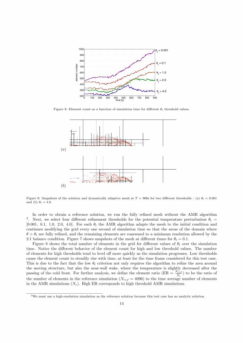
Figure 8: Element count as a function of simulation time for different θt threshold values.

(a)

(b)

Figure 9: Snapshots of the solution and dynamically adaptive mesh at T = 900s for two different thresholds : (a) θt = 0.001and (b) θt = 4.0.

In order to obtain a reference solution, we run the fully refined mesh without the AMR algorithm3. Next, we select four different refinement thresholds for the potential temperature perturbation θt =[0.001, 0.1, 1.0, 2.0, 4.0]. For each θt the AMR algorithm adapts the mesh to the initial condition andcontinues modifying the grid every one second of simulation time so that the areas of the domain whereθ > θt are fully refined, and the remaining elements are coarsened to a minimum resolution allowed by the2:1 balance condition. Figure 7 shows snapshots of the mesh at different times for θt = 0.1.

Figure 8 shows the total number of elements in the grid for different values of θt over the simulationtime. Notice the different behavior of the element count for high and low threshold values. The numberof elements for high thresholds tend to level off more quickly as the simulation progresses. Low thresholdscause the element count to steadily rise with time, at least for the time frame considered for this test case.This is due to the fact that the low θt criterion not only requires the algorithm to refine the area aroundthe moving structure, but also the near-wall wake, where the temperature is slightly decreased after thepassing of the cold front. For further analysis, we define the element ratio (ER =

Nref

Ne) to be the ratio of

the number of elements in the reference simulation (Nref = 4096) to the time average number of elementsin the AMR simulations (Ne). High ER corresponds to high threshold AMR simulations.

3We must use a high-resolution simulation as the reference solution because this test case has no analytic solution.

14

Table I: Front location (L), minimum potential temperature perturbation (θmin) and simulation runtime (Ts).

RK35 BDF2 ARK2θt L [m] θmin [K] Ts [h] L [m] θmin [K] Ts [h] L [m] θmin [K] Ts [h]ref. 14758.87 -8.90603 60.94 14758.70 -8.90630 6.13 14758.87 -8.90603 9.68

0.001 14758.79 -8.90606 9.78 14758.71 -8.90650 1.08 14758.79 -8.90609 1.570.1 14758.81 -8.90607 7.85 14758.74 -8.90661 0.89 14758.81 -8.90610 1.271.0 14758.86 -8.90619 6.24 14758.89 -8.90688 0.75 14758.86 -8.90622 1.032.0 14758.89 -8.90608 5.53 14758.98 -8.90690 0.71 14758.89 -8.90611 0.924.0 14758.80 -8.90555 4.11 14759.10 -8.90648 0.57 14758.80 -8.90558 0.71

8.1.1. Accuracy Analysis

In Fig. 9 two different AMR simulation results are presented. The top picture shows the potentialtemperature perturbation field for a low threshold (θt = 0.001) simulation, while the bottom plot shows ahigh threshold (θt = 4.0) result. The main features of the solution are the same in both cases. Even thoughin the high threshold simulation the resolved region does not encompass the entire structure, the positionof the front and the rotor structure looks identical to the low threshold case. The difference can be noted inthe wake of the front and the far field. The high threshold mesh does not capture the wake well, thereforethis feature is not represented in the bottom plot.

Table I confirms that all simulations reproduce the main features of the solution well. The simulationswere run using an explicit 3rd order 5 step Runge-Kutta method (RK35), an IMEX second-order backwarddifference formula (BDF2) method and an IMEX second-order Additive Runge-Kutta method (ARK2) - see[40] for details of these time-integrators. The front position was calculated as the location of −1K isotherm atthe bottom wall. The values from the computational grid were interpolated using the visualization packageParaview to a very fine (0.01m resolution) uniform grid, and the location of the isotherm was measuredon that uniform grid. The front position error does not exceed 1m for all the methods. Interestingly, thefront location for RK35 and ARK2 methods are identical. ARK2 also closely follows RK35 with regardto the minimum potential temperature perturbation, which suggests that ARK2 delivers superior accuracyto BDF2. The BDF2 results for both the front location and minimum potential temperature perturbationgives similar, but slightly different results than RK35 and ARK2.

6 8 10 12 14 1610

−8

10−7

10−6

10−5

10−4

10−3

element ratio

L2 e

rro

r

RK35

BDF2

ARK2

Figure 10: L2 error norms for AMR simulations using different time integrators: blue line with circles shows RK35 result;green line with squares shows BDF2 result; red line with x markers shows ARK2 result.

Figure 10 shows the L2 normalized error norms for all AMR simulations plotted against the element ratio.The norm was computed by comparing the potential temperature perturbation field of the AMR simulationswith a fully refined reference case with the same time-integration method (AMR explicit compared withreference explicit - blue line with circle markers; AMR BDF2 compared with reference BDF2 - green linewith square markers; AMR ARK2 compared with reference ARK2 - red line with cross markers) using the

15

following formula:

L2(Q, q) =

∑e,k

(Qek − qek)2

∑e,k

(Qek)2, (19)

where Q is the reference solution, q is the AMR solution, e is the index traversing the elements, and kenumerates the nodal points within each element.

The error for all the time integration methods is the same, which shows that AMR equally impacts thesimulation accuracy regardless of the time integration scheme. For low ER simulations the L2 error is verysmall and stays below 10−6. For high ER the error grows to 10−4. This indicates that for low ER casesthe entire domain is adequately resolved, while for high ER simulations the unresolved far field impacts theglobal accuracy of the solution.

Overall, the error analysis shows that AMR can deliver an accurate result, with the level of accuracydependent on the refinement threshold. Even the high threshold AMR simulations can represent the mainfeatures of the solution well. Regarding IMEX methods, ARK2 seems to deliver more accurate solutions(i.e. the solution which is closer to the explicit RK35).

8.1.2. Performance Analysis

We examine the performance of three time integration methods in conjunction with an adaptive mesh:the explicit RK35, IMEX BDF2, and IMEX ARK2 methods. While the explicit method proves to be simplerto analyze, IMEX is the method of choice for all real-world applications, because it relaxes the explicit timestep constraint. For explicit simulations the time step (∆t = 0.01s) was ten times smaller than for the IMEXsimulations. Figure 11d reflects that difference, as the IMEX simulations run nearly 10 times faster thantheir explicit counterparts. The fastest method is the BDF2, while the ARK2 is just slightly slower runningwith the same time step (although the ARK2 method can use a larger time-step than BDF2 due to a largerstability region). The Courant number for the IMEX simulations was 1.6.

Since the AMR simulations have a lower element count, we expect them to run proportionally fasterthan a fully refined reference simulation. The theoretical ideal speed-up is equal to the ratio of the numberof elements in the reference case to an average number of elements in the AMR simulations. We expectthat the AMR algorithm incurs an overhead for the evaluation of the refinement criterion, projection ofthe solution between dynamically changing meshes and computation of non-conforming fluxes, therefore theactual speed-up curve should never exceed the ideal profile. The difference between the ideal and actualspeed-up curves is a measure of the AMR overhead.

Figure 11 shows the speed-up of the AMR algorithm for different ER values for (a) explicit RK35, (b)IMEX BDF2 and (c) all three time integration methods. The black solid line without markers represents theideal theoretical speed-up. The speed-up of explicit AMR simulations (blue solid line with circular markersin Fig. 11a) is nearly ideal, which indicates that the cost of performing all the operations accredited toAMR is negligible compared to the cost of time integration. Since in this case the refinement criterion wasevaluated every second (i.e., every 100 time-steps) we plot the speed-up of the simulation with refinementcheck every time-step in the blue dashed line. The overhead due to frequent criterion evaluation showson the plot, but is still very small. This also indicates that the leading cost in the AMR overhead is theevaluation of the criterion, since when we take away the majority of that cost (solid blue line with circularmarkers) the speed-up curve overlaps with the ideal line. The other components of the overhead (meshmanipulations, data projections, non-conforming flux computations) have a negligible cost.

In order to validate the choice of refinement frequency, we plot in Fig. 12 the time history of the elementcount for two extreme refinement thresholds using refinement every time-step (black lines) and every onesecond (100 time steps for explicit, or 10 time steps for IMEX simulations). Both curves overlap - onlysmall differences are visible for the high threshold simulation near time T = 680s, which can be attributedto ”blinking”, that is refining and de-refining the same mesh location every time step. In this case the lessfrequent refinement works to our advantage by removing this unwelcome feature.

16

(a) (b)

6 8 10 12 14 16

6

8

10

12

14

16

element ratio

speed−

up

6 8 10 12 14 16

6

8

10

12

14

16

element ratio

speed−

up

(c) (d)

6 8 10 12 14 16

6

8

10

12

14

16

element ratio

sp

ee

d−

up

ideal

BDF2

ARK2

RK35

102

103

104

103

104

105

106

average element number

wall

tim

e [s]

BDF2

RK35

ARK2

Figure 11: Speed-up for (a) RK35, (b) BDF2 and (c) all time-integrators. Black solid line without markers indicates idealspeed-up. Blue line with circles marks the RK35 results, green line with squares marks BDF2 and red line with crosses marksARK2. (a) Dashed line shows the speed-up in the case where the refinement criterion is evaluated at every iteration. (b)The dashed line shows the speed-up with a constant number of solver iterations. (d) Wall clock time for all time integrationmethods.

In Fig. 11b the green solid line with square markers represents simulations with IMEX BDF2 timeintegration. Clearly the overhead incurred by adaptive simulations is much greater than in the explicitcase. The speed-up curve has a variable slope, which indicates that the overhead changes with the choiceof refinement threshold. The speed-up of AMR simulations with the IMEX ARK2 method (red line withcross markers in Fig. 11c) is much better than the BDF2, but with bigger overhead than the RK35. Alsothe slope for ARK2 seems to be less variable than for BDF2.

At the heart of our IMEX methods is the GMRES iterative solver. In Fig. 13 we show the average numberof GMRES iterations per time step as a function of ER for both BDF2 (green line with square markers) andARK2 (red line with cross markers). The point corresponding to ER = 1 is the reference simulation. ForBDF2 the average iteration count grows with ER, while for ARK2 it remains more or less constant. Thiscan explain the difference in the overhead incurred by AMR with those two time integration methods. Toinvestigate the matter further we run the BDF2 simulations with a prescribed number of GMRES iterations.The result of this exercise is depicted by the dashed line in Fig. 11b. The nearly ideal speed-up is regainedby introducing a constant number of GMRES iterations for each simulation. Of course such a constraintis artificial, as the GMRES algorithm automatically determines the number of iterations needed to satisfythe solution accuracy. This means, however, that it is indeed the variable GMRES iteration count that ispreventing the AMR BDF2 simulations from achieving a good speed-up.

To investigate the reason for the higher average number of iterations per time step in the AMR BDF2simulations we plot the time history of the iteration count for both the reference and θt = 0.001 simulationsin Fig. 14a. The top plot shows the GMRES iterations for the reference simulation - the number oscillatesbetween 7 and 8 every time step. The bottom plot represents the AMR simulation and reveals frequent

17

0 100 200 300 400 500 600 700 800 900200

300

400

500

600

700

800

900

1000

time [s]

ele

me

nt

co

un

t

Figure 12: Element number time history for two different refinement threshold settings (θt = 0.001 top line; θt = 4.0 bottomline) evaluating the criterion every time step (black) and every 100 time steps (green) with RK35.

0 5 10 157

7.5

8

8.5

9

9.5

10

10.5

element ratio

avg

. G

MR

ES

ite

ratio

ns

BDF2

ARK2

Figure 13: Average number of GMRES iteration per time step for reference and adaptive simulations.

spikes in the iteration count. A closer look at the iteration count compared with the changes in the numberof elements in the mesh (Fig. 14b) shows that the spike in the iteration count occurs whenever there is achange in the mesh. This clearly implies that the AMR algorithm incurs an additional overhead with theIMEX BDF2 method because of an increased number of GMRES iterations.

On the other hand, such spikes do not occur for ARK2. The iteration count history in Fig. 14c is verysimilar for both the reference and θt = 0.001 simulations, however much more variable compared with theBDF2 reference. The reason for the different behavior is that even though both BDF2 and ARK2 use thesame iterative solver, the system solved by GMRES actually differs between the two methods. While notexhaustive, this result does seem to show that BDF2 is less robust than ARK2 with respect to the projectionsof the solution between meshes that is introduced by the AMR algorithm. One simple explanation is thatBDF2 is a multi-step method (requires the solution at two time-levels in addition to the right-hand-sidevector) while ARK2 is a single-step multi-stage method (which only requires the solution at one previoustime level and all stages are built directly from this).

8.1.3. Mass conservation

An important measure of the quality of the discretization is the mass conservation. In order to showthat our non-conforming AMR implementation does conserve mass as well as a conforming DG method, weinvestigate the mass conservation error. We define the mass conservation error as:

M(t) =m(0)−m(t)

m(0), (20)

18

(a) (b)

5

10

15

20

k

0 100 200 300 400 500 600 700 800 9005

10

15

20

time [s]

k

5

10

15

k

480 485 490 495 500620

640

660

time [s]

Ne

(c)

0 100 200 300 400 500 600 700 800 9004

6

8

10

time [s]

k

0 100 200 300 400 500 600 700 800 9004

6

8

10

time [s]

k

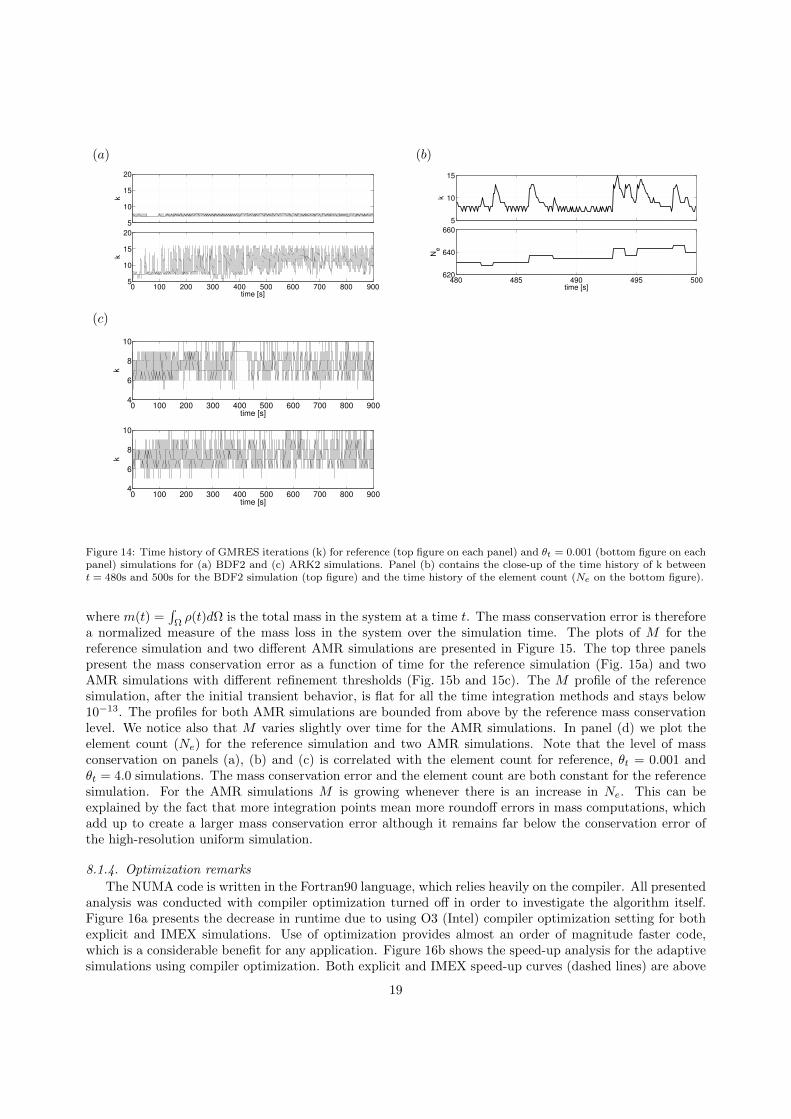
Figure 14: Time history of GMRES iterations (k) for reference (top figure on each panel) and θt = 0.001 (bottom figure on eachpanel) simulations for (a) BDF2 and (c) ARK2 simulations. Panel (b) contains the close-up of the time history of k betweent = 480s and 500s for the BDF2 simulation (top figure) and the time history of the element count (Ne on the bottom figure).

where m(t) =∫

Ωρ(t)dΩ is the total mass in the system at a time t. The mass conservation error is therefore

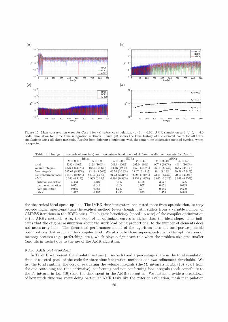
a normalized measure of the mass loss in the system over the simulation time. The plots of M for thereference simulation and two different AMR simulations are presented in Figure 15. The top three panelspresent the mass conservation error as a function of time for the reference simulation (Fig. 15a) and twoAMR simulations with different refinement thresholds (Fig. 15b and 15c). The M profile of the referencesimulation, after the initial transient behavior, is flat for all the time integration methods and stays below10−13. The profiles for both AMR simulations are bounded from above by the reference mass conservationlevel. We notice also that M varies slightly over time for the AMR simulations. In panel (d) we plot theelement count (Ne) for the reference simulation and two AMR simulations. Note that the level of massconservation on panels (a), (b) and (c) is correlated with the element count for reference, θt = 0.001 andθt = 4.0 simulations. The mass conservation error and the element count are both constant for the referencesimulation. For the AMR simulations M is growing whenever there is an increase in Ne. This can beexplained by the fact that more integration points mean more roundoff errors in mass computations, whichadd up to create a larger mass conservation error although it remains far below the conservation error ofthe high-resolution uniform simulation.

8.1.4. Optimization remarks

The NUMA code is written in the Fortran90 language, which relies heavily on the compiler. All presentedanalysis was conducted with compiler optimization turned off in order to investigate the algorithm itself.Figure 16a presents the decrease in runtime due to using O3 (Intel) compiler optimization setting for bothexplicit and IMEX simulations. Use of optimization provides almost an order of magnitude faster code,which is a considerable benefit for any application. Figure 16b shows the speed-up analysis for the adaptivesimulations using compiler optimization. Both explicit and IMEX speed-up curves (dashed lines) are above

19

(a) (b)

0 100 200 300 400 500 600 700 800 90010

−16

10−15

10−14

10−13

10−12

time [s]

M1

RK35

BDF2

ARK2

0 100 200 300 400 500 600 700 800 90010

−16

10−15

10−14

10−13

10−12

time [s]

M1

RK35

BDF2

ARK2

(c) (d)

0 100 200 300 400 500 600 700 800 90010

−16

10−15

10−14

10−13

10−12

time [s]

M1

RK35

BDF2

ARK2

0 100 200 300 400 500 600 700 800 90010

2

103

104

time [s]

Nel

θt = 4.0

θt = 0.001

reference

Figure 15: Mass conservation error for Case 1 for (a) reference simulation, (b) θt = 0.001 AMR simulation and (c) θt = 4.0AMR simulation for three time integration methods. Panel (d) shows the time history of the element count for all threesimulations using all three methods. Results from different simulations with the same time-integration method overlap, whichis expected.

Table II: Timings (in seconds of runtime) and percentage breakdown of different AMR components for Case 1.

RK35 BDF2 ARK2θt = 0.001 θt = 4.0 θt = 0.001 θt = 4.0 θt = 0.001 θt = 4.0

total 5292 (100%) 2128 (100%) 643.6 (100%) 297.0 (100%) 967.8 (100%) 403.1 (100%)volume integrals 2876.1 (54.3%) 1183.3 (55.6%) 274.46 (42.6%) 135.2 (45.5%) 362.9 (37.5%) 153.7 (38.1%)face integrals 507.67 (9.59%) 182.19 (8.56%) 66.59 (10.3%) 28.07 (9.45 %) 80.1 (8.29%) 29.58 (7.34%)non-conforming faces 116.79 (2.21%) 90.94 (4.27%) 21.33 (3.31%) 20.98 (7.06%) 23.65 (2.44%) 20.14 (4.99%)AMR: 6.030 (0.11%) 2.933 (0.14%) 6.291 (0.98%) 3.154 (1.06%) 6.025 (0.62%) 3.037 (0.75%)

criterion evaluation 3.463 1.422 3.517 1.468 3.527 1.506mesh manipulation 0.051 0.049 0.05 0.057 0.051 0.063data projection 0.965 0.581 1.247 0.77 0.965 0.599other 1.412 0.787 1.450 0.833 1.454 0.843

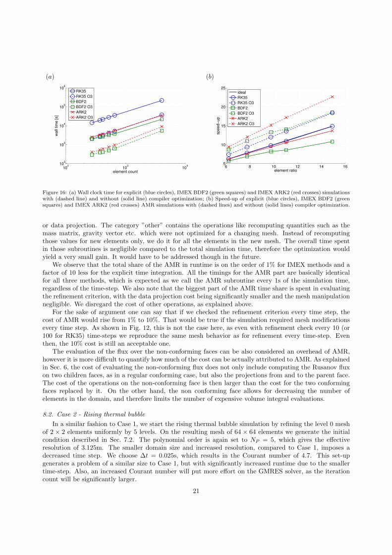
the theoretical ideal speed-up line. The IMEX time integrators benefitted more from optimization, as theyprovide higher speed-ups than the explicit method (even though it still suffers from a variable number ofGMRES iterations in the BDF2 case). The biggest beneficiary (speed-up wise) of the compiler optimizationis the ARK2 method. Also, the slope of all optimized curves is higher than the ideal slope. This indi-cates that the original assumption about the work load being proportional to the number of elements doesnot necessarily hold. The theoretical performance model of the algorithm does not incorporate possibleoptimizations that occur at the compiler level. We attribute those super-speed-ups to the optimization ofmemory accesses (e.g., prefetching, etc.), which plays a significant role when the problem size gets smaller(and fits in cache) due to the use of the AMR algorithm.

8.1.5. AMR cost breakdown

In Table II we present the absolute runtime (in seconds) and a percentage share in the total simulationtime of selected parts of the code for three time integration methods and two refinement thresholds. Welist the total runtime, the cost of evaluating the volume integrals (the Ωe integrals in Eq. (10) apart fromthe one containing the time derivative), conforming and non-conforming face integrals (both contribute tothe Γe integral in Eq. (10)) and the time spent in the AMR subroutine. We further provide a breakdownof how much time was spent doing particular AMR tasks like the criterion evaluation, mesh manipulation

20

(a) (b)

102

103

104

102

103

104

105

106

element count

wa

ll tim

e [

s]

RK35

RK35 O3

BDF2

BDF2 O3

ARK2

ARK2 O3

6 8 10 12 14 165

10

15

20

25

element ratio

sp

ee

d−

up

ideal

RK35

RK35 O3

BDF2

BDF2 O3

ARK2

ARK2 O3

Figure 16: (a) Wall clock time for explicit (blue circles), IMEX BDF2 (green squares) and IMEX ARK2 (red crosses) simulationswith (dashed line) and without (solid line) compiler optimization; (b) Speed-up of explicit (blue circles), IMEX BDF2 (greensquares) and IMEX ARK2 (red crosses) AMR simulations with (dashed lines) and without (solid lines) compiler optimization.

or data projection. The category ”other” contains the operations like recomputing quantities such as themass matrix, gravity vector etc. which were not optimized for a changing mesh. Instead of recomputingthose values for new elements only, we do it for all the elements in the new mesh. The overall time spentin those subroutines is negligible compared to the total simulation time, therefore the optimization wouldyield a very small gain. It would have to be addressed though in the future.

We observe that the total share of the AMR in runtime is on the order of 1% for IMEX methods and afactor of 10 less for the explicit time integration. All the timings for the AMR part are basically identicalfor all three methods, which is expected as we call the AMR subroutine every 1s of the simulation time,regardless of the time-step. We also note that the biggest part of the AMR time share is spent in evaluatingthe refinement criterion, with the data projection cost being significantly smaller and the mesh manipulationnegligible. We disregard the cost of other operations, as explained above.

For the sake of argument one can say that if we checked the refinement criterion every time step, thecost of AMR would rise from 1% to 10%. That would be true if the simulation required mesh modificationsevery time step. As shown in Fig. 12, this is not the case here, as even with refinement check every 10 (or100 for RK35) time-steps we reproduce the same mesh behavior as for refinement every time-step. Eventhen, the 10% cost is still an acceptable one.

The evaluation of the flux over the non-conforming faces can be also considered an overhead of AMR,however it is more difficult to quantify how much of the cost can be actually attributed to AMR. As explainedin Sec. 6, the cost of evaluating the non-conforming flux does not only include computing the Rusanov fluxon two children faces, as in a regular conforming case, but also the projections from and to the parent face.The cost of the operations on the non-conforming face is then larger than the cost for the two conformingfaces replaced by it. On the other hand, the non conforming face allows for decreasing the number ofelements in the domain, and therefore limits the number of expensive volume integral evaluations.

8.2. Case 2 - Rising thermal bubble

In a similar fashion to Case 1, we start the rising thermal bubble simulation by refining the level 0 meshof 2 × 2 elements uniformly by 5 levels. On the resulting mesh of 64 × 64 elements we generate the initialcondition described in Sec. 7.2. The polynomial order is again set to NP = 5, which gives the effectiveresolution of 3.125m. The smaller domain size and increased resolution, compared to Case 1, imposes adecreased time step. We choose ∆t = 0.025s, which results in the Courant number of 4.7. This set-upgenerates a problem of a similar size to Case 1, but with significantly increased runtime due to the smallertime-step. Also, an increased Courant number will put more effort on the GMRES solver, as the iterationcount will be significantly larger.

21

0 100 200 300 400 500 600 700200

400

600

800

1000

1200

1400

1600

1800

time [s]

Ne

θt = 0.001

θt = 0.01

θt = 0.1

θt = 0.3

Figure 17: History of element count for different refinement threshold settings for Case 2.

Table III: Maximum potential temperature perturbation (θmax), height of the bubble (Hb) and simulation runtime (Ts).

RK35 BDF2 ARK2θt Hb [m] θmax [K] Ts [h] Hb [m] θmax [K] Ts [h] Hb [m] θmax [K] Ts [h]ref. 961.09 0.46110 197.51 960.16 0.46124 91.29 961.27 0.46064 77.38

0.001 961.07 0.46110 58.51 960.75 0.46012 28.50 961.74 0.45993 23.640.01 961.05 0.46116 49.67 960.88 0.46031 25.79 961.81 0.46001 19.990.1 962.27 0.46049 35.48 962.15 0.45861 19.43 963.02 0.45853 14.980.35 968.92 0.45795 18.13 967.76 0.45551 10.22 968.34 0.45759 7.95

Figure 17 shows the time history of the element count for four different refinement thresholds. Thebehavior of the mesh is similar to Case 1; the mesh initially does not change much. The number of elementsstarts growing at later times. For high thresholds this growth is subsequently stopped (θt = 0.3 for t > 600s).The period of the initial inactivity is longer by 100s than for Case 1, and has a much larger share in thetotal simulation time (over 50%).

8.2.1. Accuracy analysis

Figure 18 compares four potential temperature perturbation fields at t = 700s for different refinementthresholds. Figure 18a shows that the lowest threshold refines a large portion of the domain around thebubble, including the interior of the mushroom bubble and the wake. This results in very smooth contourlines. As the threshold rises, a smaller portion of the domain is refined and the contours become more wavyindicating some instability. Note that in Figs. 18b and 18c we see that the outer contours of the mushroomare refined in the same way, but the mesh within the bubble is very different, which results in a more wavymushroom pattern in Fig. 18c. This indicates that not only the strong gradient zone, but also the internalmushroom region is important for this case. The solution in Fig. 18d is the worst case scenario where thegeneral bubble shape is still recreated, but the solution is not smooth and some mesh imprinting can beseen at the interfaces of big elements in the center of the mushroom. In this case only the highest potentialtemperature perturbation areas are refined and the lack of refinement in the rest of the bubble affects thesolution in the refined region significantly.

Table III summarizes the maximum potential temperature perturbation in the domain at time T = 700s,as well as the position (height) of the bubble at that time. The position of the bubble is defined as avertical coordinate of the top-most cross-section of θ = 0.1K isoline and x = 500m central axis of thebubble. Additionally the runtime for all the cases using different time integration methods is presented forcomparison. The runtime was measured for simulations without compiler optimizations and preconditioning.

For all time integration methods, both the bubble height and θmax follow the reference solution closelyfor low θt and diverge for larger values of the refinement threshold. The simulation with θt = 0.01 matches

22

(a) (b)

(c) (d)

Figure 18: Potential temperature perturbation contours at t = 700s for (a) θt = 0.001, (b) θt = 0.01, (c) θt = 0.1, and (d)θt = 0.35.

the reference solution almost perfectly, but obtains this result in a significantly shorter simulation time( 25%). In this case IMEX methods run with a significantly higher Courant number than in Case 1, whichcauses the reference simulations for both BDF2 and ARK2 to differ slightly from the explicit one. Similarly,the AMR results for both ARK2 and BDF2 are not exactly the same as their explicit counterparts. TheARK2 method proves to be the fastest among the three.

In Fig. 19 the L2 norms of the potential temperature perturbation for two IMEX methods are presented.The norms were computed using the reference simulation for each method (BDF2 AMR simulations com-pared with BDF2 reference, likewise for ARK2). Similarly to the Case 1 results, the error does not differmuch among methods, which indicates that AMR affects the accuracy of both methods in the same way. Thelevel of error is significantly higher, though, than in the density current case. This is because the artificialviscosity applied to stabilize this flow is significantly smaller than for the density current case. Typicallythe viscosity for Case 1 is µ = 75m2/s while for Case 2 it is µ = 0.1m2/s. This amount of viscosity isenough to stabilize the flow, but is barely enough to guarantee a smooth solution for the effective resolutionof ∆x = 3.125m (see [32]). A more in-depth analysis of the rising thermal bubble case with AMR will followin an upcoming paper.

8.2.2. Performance analysis

Figure 20 shows the simulation runtime (Fig. 20a) and speed-up (Fig. 20b) of AMR simulations fordifferent refinement thresholds. Solid lines represent unoptimized simulations, while dashed lines show the

23

3 4 5 6 7 8 9 10 11 1210

−4

10−3

10−2

10−1

element ratio

L2

BDF2

ARK2

RK35

Figure 19: L2 error norms for RK35 (blue line with circles), BDF2 (green line with squares) and ARK2 (red line with crosses)for Case 2.

(a) (b)

102

103

104

103

104

105

106

element count

wa

ll tim

e [

s]

BDF2 O3

ARK2 O3

BDF2

ARK2

RK35 O3

RK35

3 4 5 6 7 8 9 10 11 122

4

6

8

10

12

14

16

18

element ratio

sp

ee

d−

up

ideal

BDF2 O3

ARK2 O3

RK35 O3

ARK2

BDF2

RK35

Figure 20: (a) Wall clock time as a function of average element count and (b) speed-up of AMR simulations as a function ofER for different IMEX methods for Case 2. Green line with squares represents BDF2; red line with crosses shows the result forARK2; blue line with circles marks the timing of the explicit RK35 method. Dashed lines represent the code optimized usingcompiler flags, solid lines show the unoptimized case. The solid black line shows the expected ideal speed-up.

performance of the compiler O3 optimizations. As observed already in Table III, ARK2 was the fastestone for this case for both optimized and unoptimized runs. The speed-up plot for unoptimized simulationslooks similar to those for Case 1, where explicit RK35 obtains nearly ideal speed-up, followed by ARK2 andBDF2. This time the difference between IMEX methods is not as pronounced. The compiler optimized runsagain show speed-ups exceeding expectations.

The greater speed of ARK2 simulations can be credited to an increased Courant number (comparedto Case 1) and the absence of preconditioning. ARK2 is a two stage method, where each of the stagesperforms significantly less GMRES iterations than a single BDF2 time-step. The total number of iterationsper time step is presented in Fig. 21. Since the cost of GMRES is O(k2) (where k is the number of GMRESiterations) that alone accounts for an increased runtime. On the other hand, the use of preconditionerscould significantly bring down the number of iterations for BDF2, while ARK2 may not benefit as muchdue to the relatively small iteration count at each stage. We discuss the impact of preconditioners in thefollowing section.

Figure 21 shows the average number of GMRES iterations for both IMEX methods. For ARK2 wepresent the sum of iterations from both implicit stages. In both cases AMR causes the increase of theiteration count, however it is much more pronounced for the BDF2 method. Contrary to the Case 1 result,this does not translate into a significant difference in the speed-up plots.

Looking at Fig. 22 we see that the previously reported spikes in the GMRES iteration count (for Case

24

0 2 4 6 8 10 1228

30

32

34

36

38

40

42

element ratio

avg

. G

MR

ES

ite

ratio

ns

BDF2

ARK2

Figure 21: Average number of GMRES iterations as a function of ER for different IMEX methods for Case 2. Green line withsquares represents BDF2; red line with crosses shows the result for ARK2.

1) are not as significant for Case 2. The iteration count for the BDF2 AMR simulation (bottom plot of Fig.22a) is larger compared to the reference case (top plot). The spikes, however, mainly occur while de-refiningthe mesh (Fig. 22b) and do not significantly contribute to the overall average iteration count. Very smallspikes can be noted when the element count increases, but compared to the average iteration number thisincrease is negligible. For ARK2 the AMR GMRES iteration time history (bottom plot of Fig. 22c) muchmore closely follows the reference case (top plot of Fig. 22c), which indicates more robustness of this methodwith respect to the AMR algorithm.

8.2.3. Preconditioning

In any real application IMEX methods are used in combination with a preconditioner in order to im-prove the conditioning of the system and bring the GMRES iteration count down. Of course, the cost ofcomputing and applying the preconditioner has to be smaller than the cost saved by decreasing the iterationcount. An added complexity occurs in the AMR case, because the mesh keeps changing and therefore thepreconditioner has to adapt to those changes. Here we present only a very preliminary discussion of the useof preconditioners in the AMR simulations. We apply the element-based spectrally-optimized approximateinverse preconditioner described in [41].

Figure 23 presents the GMRES iteration count for both IMEX methods with preconditioning (dashedline) and without (solid line). For both BDF2 and ARK2, the preconditioner brought down the number ofiterations by a similar factor. The decrease of the iteration count does not translate to decrease in runtimefor both methods equally well, which can be observed in Fig. 24a. For BDF2 the use of preconditioningresulted in noticeably faster simulations, while for ARK2 the speed-up was not as pronounced. Interestingly,the reference simulations benefitted more from the preconditioner (the rightmost points on the graph). Thisis due to the fact that without AMR the preconditioner has to be computed only once at the beginning ofthe simulation and does not need to be recomputed. For AMR simulations the recomputing of the precon-ditioner adds a significant overhead. It is apparent in Fig. 24b, where the speed-up lines for preconditionedsimulations are significantly lower than the speed-up for non-preconditioned cases.

It is worth noting that this is just a preliminary study of the influence of preconditioning on the AMRsimulations. At the moment we recompute the preconditioner each time the mesh is modified, even if onlyone of the elements is changed. Further study will reveal if it is possible to limit this overhead. Additionally,this preconditioner was designed for the Schur-form CG method and is applied to no-Schur form DG method,therefore it may not be as beneficial for the cases at hand. We will address these issues in an upcomingpaper.

8.2.4. Mass conservation

Similarly to Case 1, the mass conservation error for the AMR simulations for Case 2 is bounded by theerror for the reference case. Figure 25 shows the same sensitivity of M to an increasing number of elements

25

(a) (b)

20

30

40

50

k

0 100 200 300 400 500 600 70020

30

40

50

time [s]

k

30

40

50

k

280 285 290 295 3001100

1150

time [s]

Ne

(c)

10

20

30

40

k

0 100 200 300 400 500 600 70010

20

30

40

time [s]

k

Figure 22: Time history of GMRES iterations (k) for reference (top figure on each panel) and θt = 0.1 (bottom figure on eachpanel) simulations for (a) BDF2 and (c) ARK2 simulation. Panel (b) contains the close-up of the time history of k betweent = 280s and 300s for BDF2 simulation (top figure) and the time history of the element count (Ne on the bottom figure).

Table IV: Corrected coefficients for the RK35 method. ∗ marks the difference from [42].

stage α β1 1 0 0 0.3772689153313682 0 1 0 0.3772689153313683 0.355909775063326∗ 0.644090224936674 0 0.2429952205373964 0.367933791638137 0.632066208361863 0 0.2384589328462905 0 0.762406163401431 0.237593836598569 0.237593836598569

over simulation time. All three time integration methods give consistent mass conservation behavior. Duringthe study an important feature of the explicit RK35 method has been noted, which can be extended to othertime integration methods. It is important that the coefficients of each stage of the Runge-Kutta method areconsistent up to a desired precision. If we aim for double precision and therefore are looking for round-offerrors at the 10−16 level, the coefficients have to be consistent up to the 16th decimal place. This is notthe case with the coefficients of the third stage of RK35 published in Ruuth [42]. In the case of this studya small inconsistency at the last decimal place, which is probably the result of a roundoff error, led to asteady growth of the M norm. In Table IV we provide consistent coefficients for the RK35 method whichfixed this steady growth.

8.2.5. AMR cost breakdown

Compared to the results for Case 1, the share of the cost of AMR for IMEX methods in Case 2 issignificantly smaller. This is because the time integration became more expensive due to the increasedCourant number. Also, the criterion evaluation cost with regards to the total AMR cost is much bigger thanin the previous case, especially for θt = 0.01 simulations. This is because we are checking the refinementcriterion every 10 iterations, which translates to 0.25s of simulation time. We therefore check for refinementmore often than actually perform any mesh modification. It is clear that the refinement check frequencyparameter could have been chosen more optimally. Note, however, that for this case the cost of timeintegration is so high that even more frequent checks would not cause the cost of AMR to exceed a fewpercents.

26

0 2 4 6 8 10 1210

15

20

25

30

35

40

45

element ratio

avg. G

MR

ES

ite

rations

BDF2

ARK2

AKR2 precon

BDF2 precon

Figure 23: Average number of GMRES iterations as a function of ER for different IMEX methods for Case 2 with (dashedline) and without preconditioning (solid line). Green line with squares represents BDF2; red line with crosses shows the resultfor ARK2.

(a) (b)

103

104

105

element count

wa

ll tim

e [

s]

BDF2

ARK2

BDF2 precon

ARK2 precon

2 4 6 8 10 122

4

6

8

10

12

14

16

18

element ratio

sp

ee

d−

up

ideal

BDF2

ARK2

BDF2 precon

ARK2 precon

RK35

Figure 24: (a) Runtime and (b) speed-up of compiler optimized IMEX simulations for Case 2 with (dashed line) and withoutpreconditioning (solid line). Green line with squares represents BDF2; red line with crosses shows the result for ARK2.

9. Conclusion

We presented the details of the AMR algorithm for the discontinuous Galerkin version of the Non-hydrostatic Unified Model of the Atmosphere (NUMA) and sought to analyze the benefit of AMR. To thisend, we compared the accuracy versus the speed-up of AMR with respect to uniform grid simulations.The AMR algorithm was tested using a threshold based criterion for both the density current and risingthermal bubble cases. We have investigated the performance of the AMR algorithm running with three timeintegration methods: explicit RK35 and two IMEX methods: BDF2 and ARK2. For all the methods theaccuracy of the result depends on the choice of the threshold for the refinement criterion. For higher elementratios (ER) the criterion does not capture all the features of the solution, therefore the L2 error increasesfrom 10−6 for low threshold simulations to 10−4 for high threshold ones for the density current case. Themost significant features of the solution such as the front position, minimum potential temperature or thegeneral structure of the front are captured correctly even for high ER simulations. The ARK2 methodreproduces closely the result of RK35, while BDF2 provides a less similar agreement.

For the rising thermal bubble case the general features of the solution are captured correctly by all thesimulations except the one with the highest threshold value. In that case the boundary of the bubble is

27

(a) (b)

0 100 200 300 400 500 600 70010

−16

10−15

10−14

10−13

10−12

time [s]

M1

RK35

BDF2

ARk2

0 100 200 300 400 500 600 70010

−16

10−15

10−14

10−13

10−12

time [s]

M1

RK35

BDF2

ARK2

(c) (d)

0 100 200 300 400 500 600 70010

−16

10−15

10−14

10−13

10−12

time [s]

M1

RK35

BDF2

ARK2

0 100 200 300 400 500 600 70010

2

103

104

time [s]

Nel

θt = 0.01

θt = 0.35

reference

Figure 25: Mass conservation error for Case 2 for (a) reference simulation, (b) θt = 0.01 AMR simulation and (c) θt = 0.35AMR simulation for three time integration methods. Panel (d) shows the time history of the element count for all threesimulations using all three methods. Results from different simulations with the same time-integration method overlap, whichis expected.

Table V: Timings (in seconds of runtime) and percentage breakdown of different AMR components for Case 2

RK35 BDF2 ARK2θt = 0.001 θt = 4.0 θt = 0.001 θt = 4.0 θt = 0.001 θt = 4.0

total 27994 (100%) 9710 (100%) 18938 (100%) 7154 (100%) 13245 (100%) 4687 (100%)volume integrals 13954 (49.8%) 4740 (48.8%) 4990 (26.3%) 1829 (25.6%) 4618 (34.9%) 1655 (35.3%)face integrals 2560 (9.14%) 678.9 (7%) 1540 (8.13%) 385.7 (5.39%) 1369 (10.3%) 342.6 (7.31%)non-conforming faces 677.7 (2.42%) 503.6 (5.19%) 535.4 (2.83%) 440.6 (6.16%) 460.3 (3.47%) 374.4 (7.99%)AMR: 21.7 (0.08%) 8.5 (0.09%) 22.2 (0.12 %) 8.49 (0.11%) 21.8 (0.16%) 8.29 (0.18%)

criterion evaluation 16.8 5.9 16.8 5.9 16.8 5.93mesh manipulation 0.15 0.16 0.15 0.16 0.15 0.15data projection 1.76 0.86 2.39 1.13 1.93 0.9other 2.5 1.11 2.7 1.16 2.81 1.22

clearly disturbed and some mesh artifacts are present in the solution. It was discovered that not only therefinement in the high temperature gradient area at the boundary of the bubble needs to be resolved, butthe resolution of the interior of the bubble plays a role. All the important features such as the positionof the bubble and maximum potential temperature were captured very accurately by the lower refinementthresholds at a fraction of the cost.

The performance of the algorithm was investigated by comparing the runtime and speed-up of differ-ent AMR simulations. The explicit RK35 showed nearly perfect speed-up which confirms that the AMRalgorithm is indeed very efficient. In the cases shown in the paper the overall cost of the adaptive meshalgorithm is below 1% of the total runtime. The main component of the AMR overhead is the evaluationof the refinement criterion, while the mesh manipulation and data projections have negligible cost. Forthe density current test case (Case 1) with BDF2 an additional big overhead was the increased GMRESiteration count caused by AMR. The BDF2 speed-up turned out to be the worst of all the three methods.Both IMEX methods had runtimes about an order of magnitude smaller than RK35. ARK2 was shown tobe slightly slower than BDF2 using the same time step, but with much increased accuracy and improvedspeed-up properties. The ARK2 method was shown to be more robust (less sensitive) to the changing meshcaused by the AMR algorithm. For the rising thermal bubble test case (case 2), the ARK2 was the fastest

28

method due to the increased Courant number. The difference in speed-up curves was not as pronounced,but again the ARK2 proved to have better properties and less overhead than BDF2.

In nonhydrostatic atmospheric applications (when using the fully compressible equations), IMEX meth-ods are an absolute necessity, due to a very strict constraint imposed on the explicit time-step by acousticwaves. This study shows that the performance of some IMEX methods can be affected by a dynamicallyadaptive mesh. It is important not only to design the AMR algorithm in an efficient way, but also to considerwhich time integration method to use in such applications. In our future investigations we will pursue theARK2 method due to its good performance properties and excellent accuracy.

The mass conservation error for both test cases and all the time integration methods was shown to bebounded by the mass conservation error of the reference simulations. For adaptive simulations the massconservation was affected by the changing number of elements in the mesh.

A preliminary study of the influence of preconditioning on the AMR simulations showed that it isanother significant source of overhead, mainly because the preconditioner was recomputed after every meshmodification. We will pursue the possibilities of reducing this overhead in future work since it may not benecessary to always recompute the preconditioner.

Finally, the effect of the compiler optimizations on the algorithm performance was investigated. Theoptimizations provide significant runtime reduction of the simulations, as big as a factor of 10. Additionally,optimization affects the speed-up of the AMR algorithm, as more efficient memory handling for smallerproblems allows for speed-ups greater than it would follow from the simple performance model. In a sensethe optimizations more than make up for the overhead caused by the AMR.

Acknowledgements

The authors gratefully acknowledge the support of the Office of Naval Research through program ele-ment PE-0602435N, the National Science Foundation (Division of Mathematical Sciences) through programelement 121670, and the Air Force Office of Scientific Research through the Computational Mathematicsprogram. The authors are grateful to Andreas Muller and Simone Marras for constructive discussions thatgreatly contributed to this paper.

[1] R. Nair, H.-W. Choi, H. Tufo, Computational aspects of a scalable high-order discontinuous galerkin atmospheric dynam-ical core, Comp. Fl. 38 (2) (2009) 309–319.

[2] J. Kelly, F. Giraldo, Continuous and discontinuous galerkin methods for a scalable 3d nonhydrostatic atmospheric model:limited area mode, J. Comp. Phys. 231 (2) (2012) 7988–8008.

[3] R. Hartmann, P. Houston, Adaptive discontinuous galerkin finite element methods for the compressible euler equations,J. Comp. Phys. 183 (2) (2002) 508–532.

[4] P. Bastian, M. Blatt, A. Dedner, C. Engwer, R. Klofkorn, R. Kornhuber, M. Ohlberger, O. Sander, A generic gridinterface for parallel and adaptive scientific computing. part ii: Implementation and tests in dune, Computing 82 (2-3)(2008) 121–138.

[5] C. Burstedde, O. Ghattas, M. Gurnis, G. Stadler, E. Tan, T. Tu, L. C. Wilcox, S. Zhong, Scalable adaptive mantleconvection simulation on petascale supercomputers, in: Proc. 2008 ACM/IEEE Supercomputing, IEEE Press, 2008, p. 62.

[6] C. Jablonowski, Adaptive grids in weather and climate modeling, Ph.D. thesis, The University of Michigan (2004).[7] J. Behrens, Adaptive atmospheric modeling: key techniques in grid generation, data structures, and numerical operations

with applications, Springer, 2006.[8] G. W. Ley, R. L. Elsberry, Forecasts of typhoon Irma using a nested grid model, Mon. Wea. Rev. 104 (1976) 1154.

doi:10.1175/1520-0493(1976)104¡1154:FOTIUA¿2.0.CO;2.[9] Y. Kurihara, M. A. Bender, Use of a movable nested-mesh model for tracking a small vortex, Mon. Wea. Rev. 108 (1980)

1792–1809. doi:10.1175/1520-0493(1980)108¡1792:UOAMNM¿2.0.CO;2.[10] D.-L. Zhang, H.-R. Chang, N. L. Seaman, T. T. Warner, J. M. Fritsch, A two-way interactive nesting procedure with

variable terrain resolution, Mon. Wea. Rev. 114 (7) (1986) 1330–1339.[11] G. S. Dietachmayer, K. K. Droegemeier, Application of continuous dynamic grid adaptation techniques to meteorological

modeling. i: Basic formulation and accuracy, Mon. Wea. Rev. 120 (8) (1992) 1675–1706.[12] J. M. Prusa, P. K. Smolarkiewicz, An all-scale anelastic model for geophysical flows: dynamic grid deformation, J. Comp.

Phys. 190 (2) (2003) 601–622.[13] C. J. Budd, W. Huang, R. D. Russell, Adaptivity with moving grids, Acta Numerica 18 (1) (2009) 111–241.[14] W. Skamarock, J. Oliger, R. L. Street, Adaptive grid refinement for numerical weather prediction, J. Comp. Phys. 80 (1)

(1989) 27–60.[15] W. C. Skamarock, J. B. Klemp, Adaptive grid refinement for two-dimensional and three-dimensional non-hydrostatic

atmospheric flow, Mon. Wea. Rev. 121 (3) (1993) 788–804.

29

[16] M. J. Berger, J. Oliger, Adaptive mesh refinement for hyperbolic partial differential equations, J. Comp. Phys. 53 (3)(1984) 484–512.

[17] M. J. Berger, P. Colella, Local adaptive mesh refinement for shock hydrodynamics, J. Comp. Phys. 82 (1) (1989) 64–84.[18] R. J. LeVeque, Wave propagation algorithms for multidimensional hyperbolic systems, J. Comp. Phys. 131 (2) (1997)

327–353.[19] N. Nikiforakis, Amr for global atmospheric modelling, in: Adaptive Mesh Refinement-Theory and Applications, Springer,

2005, pp. 505–526.[20] D. P. Bacon, N. N. Ahmad, Z. Boybeyi, T. J. Dunn, M. S. Hall, P. C. Lee, R. A. Sarma, M. D. Turner, K. T. Waight III,

S. H. Young, et al., A dynamically adapting weather and dispersion model: the operational multiscale environment modelwith grid adaptivity (omega), Mon. Wea. Rev. 128 (7) (2000) 2044–2076.

[21] P. K. Smolarkiewicz, A fully multidimensional positive definite advection transport algorithm with small implicit diffusion,J. Comp. Phys. 54 (2) (1984) 325–362.

[22] J. P. Iselin, J. M. Prusa, W. J. Gutowski, Dynamic grid adaptation using the mpdata scheme, Mon. Wea. Rev. 130 (4)(2002) 1026–1039.

[23] F. X. Giraldo, The lagrange-galerkin method for the two-dimensional shallow water equations on adaptive grids, Int. J.Numer. Meth. Fl. 33 (6) (2000) 789–832.

[24] J. Behrens, Atmospheric and ocean modeling with an adaptive finite element solver for the shallow-water equations, App.Num. Math. 26 (1) (1998) 217–226.

[25] J. Behrens, N. Rakowsky, W. Hiller, D. Handorf, M. Lauter, J. Papke, K. Dethloff, amatos: Parallel adaptive meshgenerator for atmospheric and oceanic simulation, Ocean Mod. 10 (1) (2005) 171–183.

[26] M. A. Taylor, A. Fournier, A compatible and conservative spectral element method on unstructured grids, J. Comp. Phys.229 (17) (2010) 5879–5895.

[27] A. St-Cyr, C. Jablonowski, J. M. Dennis, H. M. Tufo, S. J. Thomas, A comparison of two shallow water models withnon-conforming adaptive grids: classical tests, arXiv preprint physics/0702133.

[28] E. J. Kubatko, S. Bunya, C. Dawson, J. J. Westerink, Dynamic¡ i¿ p¡/i¿-adaptive runge–kutta discontinuous galerkinmethods for the shallow water equations, Comp. Meth. Appl. Mech. Engng. 198 (21) (2009) 1766–1774.

[29] D. A. Kopriva, A conservatice staggered-grid chebyshev multidomain method for compressible flows. II: A semi-stucturedmethod, Tech. Rep. 2, NASA Contractor Report (Oct. 1996). doi:10.1006/jcph.1996.0225.URL http://linkinghub.elsevier.com/retrieve/pii/S0021999196902259

[30] Y. Maday, C. Mavriplis, A. T. Patera, Nonconforming mortar element methods: Application to spectral discretizations,Institute for Computer Applications in Science and Engineering, NASA Langley Research Center, 1988.

[31] D. Rosenberg, A. Fournier, P. Fischer, A. Pouquet, Geophysical–astrophysical spectral-element adaptive refinement (gas-par): Object-oriented h-adaptive fluid dynamics simulation, J. Comp. Phys. 215 (1) (2006) 59–80.

[32] A. Mueller, J. Behrens, F. X. Giraldo, V. Wirth, An adaptive discontinuous galerkin method for modeling atmosphericconvection, J. Comp. Phys. 235 (1) (2012) 371–393.

[33] S. Brdar, M. Baldauf, A. Dedner, R. Klofkorn, Comparison of dynamical cores for nwp models: comparison of cosmo anddune, Theor. Comp. Fl. Dyn. (2012) 1–20.

[34] C. Eskilsson, An hp-adaptive discontinuous galerkin method for shallow water flows, Int. J. Numer. Meth. Fl. 67 (11)(2011) 1605–1623.

[35] S. Blaise, A. St-Cyr, A dynamic hp-adaptive discontinuous galerkin method for shallow-water flows on the sphere withapplication to a global tsunami simulation, Mon. Wea. Rev. 140 (3) (2012) 978–996.

[36] F. Giraldo, M. Restelli, A study of spectral element and discontinuous galerkin methods for the navier-stokes equations innon-hydrostatic mesoscale atmospheric modeling: equation sets and test cases, J. Comp. Phys. 227 (1) (2008) 3849–3877.

[37] C. Burstedde, O. Ghattas, M. Gurnis, T. Isaac, G. Stadler, T. Warburton, L. Wilcox, Extreme-scale amr, Proc. 2010ACM/IEEE Int. Confence for High Performance Computing, Networking, Storage and Analysis (1) (2010) 1–12.

[38] H. Sundar, R. S. Sampath, G. Biros, Bottom-up construction and 2:1 balance refinement of linear octrees in parallel,SIAM J. Sci. Comp. 30 (5) (2008) 2675–2708. doi:10.1137/070681727.URL http://epubs.siam.org/doi/abs/10.1137/070681727

[39] J. Straka, R. B. Wilhelmson, J. R. Anderson, K. K. Droegemeier, Numerical solutions of a non-linear density current: abenchmark solution and comparisons, Int. J. Numer. Meth. Fl. 17 (1993) 1–22.

[40] F. Giraldo, J. Kelly, E. Constantinescu, Implicit-explicit formulations for a 3d nonhydrostatic unified model of the atmo-sphere (numa), SIAM J. Sci. Comp. (1).

[41] L. E. Carr, C. F. Borges, F. X. Giraldo, An element-based spectrally-optimized approximate inverse preconditioner forthe euler equations, SIAM J. Sci. Comp. 34 (2012) B392–B420.

[42] S. Ruuth, Global optimization of explicit strong-stability-preserving runge-kutta methods, Math. Comp. 75 (253) (2006)183–207.

Appendix A

1D projection

The integral projection method presented in this section was proposed by [29] for general h-p non-conforming elements. Here we describe the method applied to a specific h-non-conforming edge in 2:1balance.

30

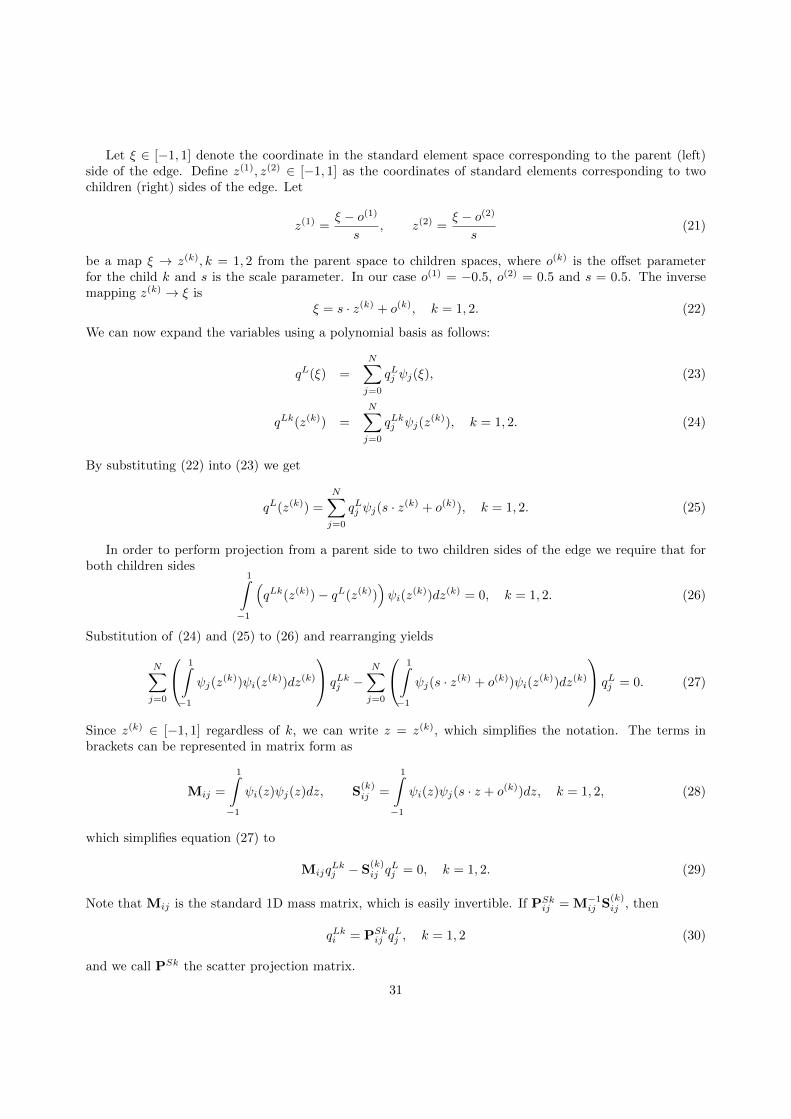
Let ξ ∈ [−1, 1] denote the coordinate in the standard element space corresponding to the parent (left)side of the edge. Define z(1), z(2) ∈ [−1, 1] as the coordinates of standard elements corresponding to twochildren (right) sides of the edge. Let

z(1) =ξ − o(1)

s, z(2) =

ξ − o(2)

s(21)

be a map ξ → z(k), k = 1, 2 from the parent space to children spaces, where o(k) is the offset parameterfor the child k and s is the scale parameter. In our case o(1) = −0.5, o(2) = 0.5 and s = 0.5. The inversemapping z(k) → ξ is

ξ = s · z(k) + o(k), k = 1, 2. (22)

We can now expand the variables using a polynomial basis as follows:

qL(ξ) =

N∑j=0

qLj ψj(ξ), (23)

qLk(z(k)) =

N∑j=0

qLkj ψj(z(k)), k = 1, 2. (24)

By substituting (22) into (23) we get

qL(z(k)) =

N∑j=0

qLj ψj(s · z(k) + o(k)), k = 1, 2. (25)

In order to perform projection from a parent side to two children sides of the edge we require that forboth children sides

1∫−1

(qLk(z(k))− qL(z(k))

)ψi(z

(k))dz(k) = 0, k = 1, 2. (26)

Substitution of (24) and (25) to (26) and rearranging yields

N∑j=0

1∫−1

ψj(z(k))ψi(z

(k))dz(k)

qLkj −N∑j=0

1∫−1

ψj(s · z(k) + o(k))ψi(z(k))dz(k)

qLj = 0. (27)

Since z(k) ∈ [−1, 1] regardless of k, we can write z = z(k), which simplifies the notation. The terms inbrackets can be represented in matrix form as

Mij =

1∫−1

ψi(z)ψj(z)dz, S(k)ij =

1∫−1

ψi(z)ψj(s · z + o(k))dz, k = 1, 2, (28)

which simplifies equation (27) to

MijqLkj − S

(k)ij q

Lj = 0, k = 1, 2. (29)

Note that Mij is the standard 1D mass matrix, which is easily invertible. If PSkij = M−1ij S

(k)ij , then

qLki = PSkij qLj , k = 1, 2 (30)

and we call PSk the scatter projection matrix.

31

Similarly the gather projection from two children sides to a parent side is performed (see Fig. 5b). Werequire that on the parent side of the face

1∫−1

(qR(ξ)− qR(ξ)

)ψi(ξ)dξ = 0, (31)

where qR is the continuous projection of the variables qR1 and qR2 from children sides to a parent side, and

qR(ξ) =

qR1(z(1)) = qR1(ξ−o(1)

s

)for − 1 ≤ ξ ≤ 0−,

qR2(z(2)) = qR2(ξ−o(2)

s

)for 0+ ≤ ξ ≤ 1.

(32)

Note that qR(ξ) allows for a discontinuity at ξ = 0. Substituting (32) into (31) yields

0∫−1

(qR(ξ)− qR1

(ξ − o(1)

s

))ψi(ξ)dξ +

1∫0

(qR(ξ)− qR2

(ξ − o(2)

s

))ψi(ξ)dξ = 0,

Using an expansion analogous to (24), (25) and rearranging we get 1∫−1

ψi(ξ)ψj(ξ)dξ

qRj −

0∫−1

ψi(ξ)ψj

(ξ − o(1)

s

)dξ

qR1j −

1∫0

ψi(ξ)ψj

(ξ − o(2)

s

)dξ

qR2j = 0.

We introduce the variable change ξ = s · z + o(k), dξ = s · dz to the second and third integral, that gives 1∫−1

ψi(ξ)ψj(ξ)dξ

qRj − s2∑k=1

1∫−1

ψi(s · z + o(k))ψj(z)dz

qRkj = 0. (33)

Note that the term in brackets to the left of qRkj is the transpose of S(k)ij defined in (??). We can write the

integrals in matrix notation:

MijqRj − s

2∑k=1

S(k)ij

TqRkj = 0, (34)

where Mij is the mass matrix as defined in (28).Finally, if we define PGkij = s ·M−1ij S

(k)lj

Tto be the gather

projection matrix, then

qRi =

2∑k=1

PGkij qRkj . (35)

2D projection

The 2D projection presented here is a two-dimensional extension of the integral projection methodpresented in the previous section.

Figure 6 presents the standard element corresponding to the parent element with coordinates (ξ, η) ∈[−1, 1]2 and four children, each with separate coordinates (z

(k)1 , z

(k)2 ) ∈ [−1, 1]2, where k = 1, . . . , 4. We

define a map:

z(k)1 =

ξ − o(k)1

s,

z(k)2 =

η − o(k)2

s, (36)

32

where o(k)1 and o

(k)2 are offset parameters corresponding to each child element k and coordinate z1 and z2.

The inverse mapping is now

ξ = s · z(k)1 + o

(k)1 , (37)

η = s · z(k)2 + o

(k)2 , (38)

where k = 1, . . . , 4, the scale parameter s = 0.5 and offsets o(k)i = ±0.5 depending on direction i and element

number k.Each element has a polynomial basis defined in which we expand the projected variable,

qP (ξ, η) =

MN∑j=1

qPj ψj(ξ, η), (39)

qCk(z(k)1 , z

(k)2 ) =

MN∑j=1

qCkj ψj(z(k)1 , z

(k)2 ), (40)

where qP is the parent element variable and qCk is the k-th child element variable projected from qP , andMN is the number of nodal points in the element. Similarly as in Equation (25) we can substitute theinverse map (37) to (39) and represent the parent variable in terms of the children coordinate system.

qP (ξ, η) = qP (z(k)1 , z

(k)2 ) =

MN∑j=1

qPj ψj(s · z(k)1 + o

(k)1 , s · z(k)

2 + o(k)2 ), k = 1, . . . , 4. (41)

For each k = 1, . . . , 4 we require that

1∫−1

1∫−1

(qCk(z

(k)1 , z

(k)2 )− qP (z

(k)1 , z

(k)2 ))ψj(z

(k)1 , z

(k)2 )dz

(k)1 dz

(k)2 = 0. (42)

Substituting expansions (39), (40), rearranging and employing matrix notation yields

MijqCkj − S

(k)ij q

Pj = 0, (43)

where

Mij =

1∫−1

1∫−1

ψj(z1, z2)ψi(z1, z2)dz1dz2, (44)

S(k)ij =

1∫−1

1∫−1

ψj(s · z1 + o(k)1 , s · z2 + o

(k)2 )ψi(z1, z2)dz1dz2. (45)

The projection matrix is once again constructed by inverting the mass matrix and left-multiplying the inversewith Eq. (43). This yields

qCki = (PSk2D)ijqPj , k = 1, . . . , 4, (46)

wherePSk2D = M−1S(k). (47)

Similarly as in the case of the gather projection in the 1D non-conforming edge case, the 2D gatherprojection matrix is constructed by multiplying the inverse of the mass matrix and transpose of 2D S(k):

PGk2D = s ·M−1S(k)T , (48)

33

which yields:

qPi =

4∑k=1

(PGk2D)ijqCkj . (49)

This approach is easily extendable to 3D projections of hexahedral elements since the same tensor-productoperations are being applied in 1D, 2D, or 3D.

34