Analysis of a long record of annual maximum rainfall in Athens, Greece, and

design rainfall inferences

Demetris Koutsoyiannis

Department of Water Resources, Faculty of Civil Engineering, National Technical University,

Heroon Polytechneiou 5, GR-15780 Zografou, Athens, Greece

(dk@hydro.ntua.gr – http://www.hydro.ntua.gr/faculty/dk)

George Baloutsos

Forest Research Institute, National Agricultural Research Foundation,

Terma Alkmanus, GR-115 28, Ilissia, Athens, Greece

Abstract. An annual series of maximum daily rainfall extending through 1860-1995, i.e., 136

years, was extracted from the archives of a meteorological station in Athens. This is the

longest rainfall record available in Greece and its analysis is required for the prediction of

intense rainfall in Athens, where currently major flood protection works are under way.

Moreover, the statistical analysis of this long record can be useful for investigating more

generalised issues regarding the adequacy of extreme value distributions for extreme rainfall

analysis and the effect of sample size on design rainfall inferences. Statistical exploration and

tests based on this long record indicate no statistically significant climatic changes in extreme

rainfall during the last 136 years. Furthermore, statistical analysis shows that the

conventionally employed Extreme Value Type I (EV1 or Gumbel) distribution is

inappropriate for the examined record (especially in its upper tail), whereas this distribution

would seem as an appropriate model if fewer years of measurements were available (i.e., part

of this sample were used). On the contrary, the General Extreme Value (GEV) distribution

appears to be suitable for the examined series and its predictions for large return periods agree

with the probable maximum precipitation estimated by the statistical (Hershfield’s) method,

when the latter is considered from a probabilistic point of view. Thus, the results of the

analysis of this record agree with a recently (and internationally) expressed scepticism about

2

the EV1 distribution which tends to underestimate the largest extreme rainfall amounts. It is

demonstrated that the underestimation is quite substantial (e.g. 1:2) for large return periods

and this fact must be considered as a warning against the widespread use of the EV1

distribution for rainfall extremes.

Keywords. Extreme rainfall, Extreme value distribution, Intensity-frequency-duration

relationship, Hydrologic statistics, Flood design, Flood risk, Athens.

1. Introduction

In modern times, particularly after World War II, Athens, the capital of Greece, has been

continually urbanised, nowadays reaching a population of about four million. Unfortunately,

urbanisation has seldom been combined with concurrent infrastructure works, such as natural

channel improvement and storm drainage networks. Moreover, there are cases where

buildings were illegally constructed over or very close to ephemeral streambeds. Thus,

flooding in Athens is probably the most severe among hydrometeorological hazards in Greece

(Koukis and Koutsoyiannis, 1997). Since 1896, at least 179 lives were lost due to floods in

Athens. The most catastrophic flood events were those of 14 November 1896, 5-6 November

1961, and 2 November 1977 causing 61, 40, and 38 deaths, respectively (Nicolaidou and

Hadjichristou, 1995). The number of lives lost due to floods in Athens is greater than that due

to any other natural hazards. For example 18 deaths due to earthquakes were reported the last

century in the Attica area that surrounds Athens (Nicolaidou and Hadjichristou, 1995).

To explain the flood propensity in Athens we must refer, in addition to the above-

mentioned anthropogenic reasons, to climatological and geomorphological factors. The

climate of Athens is Mediterranean and rather dry with a mean annual temperature around

18oC, relative humidity 62% and relative sunshine duration 66%. The mean annual number of

rain days is 72 (20%) and the mean annual rainfall depth 390 mm; the (potential) evaporation

rate is more than three times the rainfall depth. The mean annual length of dry spells is 7.7

days and this value becomes 25 days in the summer months (July-September); the maximum

observed dry spell (in the period 1930-90) is about three months and a half (109 days;

summer 1961). Interestingly, the mean annual rainfall in Athens is 3-5 times lower, and the

3

mean runoff rate is at least one order of magnitude lower, than the corresponding values in the

western part of Greece. The low runoff rate in combination with the natural relief did not lead

to the formation of significant river networks and river cross-sections. However, despite of the

small annual rainfall depth, the intense flood-producing rainstorms in Athens (typically 2-4

per year) are almost as high in intensity as in other parts of Greece.

The main and most flooding prone river of Attica is Kifissos, with a catchment area of

417 km2 (including Ilissos river). Most of the urban area of the greater Athens (240 out of 330

km2) lies in this catchment. These figures indicate that 58% (= 240 / 417) of the river

catchment is urbanised, which explains why flood propensity of Athens is mainly dependent

on rainfall generated over the city. Other factors such as antecedent moisture conditions are

less important as testified by the fact that even the first occurring storm in autumn, after a

prolonged dry summer period, may produce severe flooding.

Recently, attention has been given to the construction of storm drainage networks and

improvement of natural channels in Greater Athens. Kifissos is also being improved currently

by broadening its channel. However, until now the adopted return period for the design of

such constructions is traditionally 5-10 years for the storm drainage networks and does not

exceed 20-50 years for the main streams including Kifissos. It is estimated that these values of

return period do not provide a sufficient protection level and new, more severe, design criteria

have to be established (Xanthopoulos et al., 1995) to lower the risk. In doing that, the first

step is to estimate the rainfall amount for higher return periods or lower exceedance

probabilities. Rainfall intensity values for exceedance probabilities of the order of 10–2 to 10–4

(return periods of 100 to 10 000 years) as well as those corresponding to the probable

maximum precipitation (PMP) must be known not only for the design of new constructions

but also for performing simulations of extreme flood events to obtain a sight of the possible

impacts of such events.

Numerous studies of maximum rainfall intensities in Athens have been performed. They

used empirical or statistical techniques to construct intensity-frequency-duration (idf) curves

for return periods lower than 100 years. A review of such studies was given by Hydrauliki

(1980). Typically, these studies used rainfall intensity records of several stations in Greater

4

Athens, whose lengths varied between 26 and 72 years. However, a daily rainfall record can

be constructed in Athens for a much longer period, i.e., 136 years (extending through 1860-

1995), and clearly this can be utilised for a more reliable estimation of rainfall amount for low

exceedance probabilities.

Recently, Koutsoyiannis et al. (1998) showed that records of daily maximum rainfall

depths can be combined with rain-recording data for lower durations to construct an idf

relationship of the general form

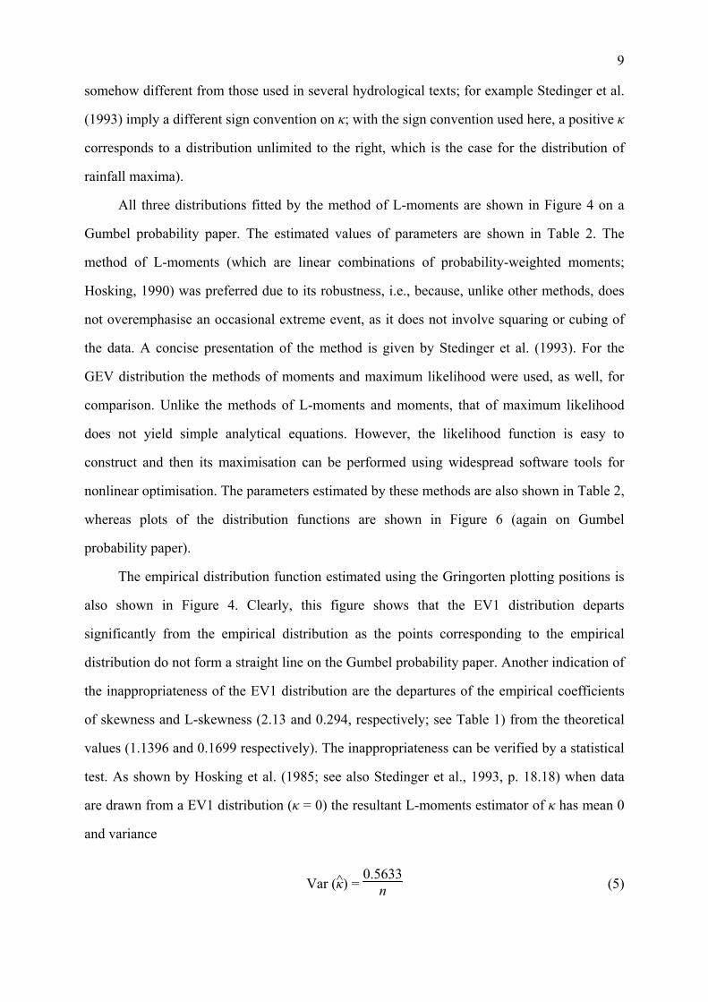
i(d, T) = a(T)b(d) (1)

where i(d, T) is the rainfall intensity corresponding to duration d and return period T, and a(T)

and b(d) functions of T and d, respectively. Particularly, they showed that the function a(T)

depends on, and can be directly derived from, the distribution function of the rainfall intensity

or rainfall depth using data of either recording or non-recording rain gauges. In addition, they

concluded that the daily observations of non-recording devices must never be ignored in

determining a(T), even in the case of coexistence of recording devices at the same station.

This is because autographic devices with their vulnerable mechanisms are more sensible to

erroneous recordings, whereas the standard non-recording rain gauges are more reliable due to

their simpler structure. Moreover, non-recording stations typically operate over periods longer

than those of recording stations and, therefore, their records lead to a more reliable estimation

of a(T). On the other hand, the determination of b(d) apparently needs rain-recording data of

lower durations down to some minutes or an hour.

The unusually large length of the record of annual maximum rainfall depth in Athens

can be utilised to investigate some issues that not necessarily apply to Athens only, but are

representative for a much wider area. Such issues are the possible changes of extreme rainfall

properties through the 136 years, and the behaviour of the distribution function in its upper

tail. We note that the record extracted for this study is the longest available one in Greece and

one of the longest in the world. For example, Wilks (1993) who investigated empirically

several distributions which are potentially suitable for describing extreme rainfall data, used

5

rainfall records of 13 stations in the U.S.A. with lengths ranging from 39 to 91 years, the

largest (91 years) being those of New York and Baltimore.

The purpose of this paper is the thorough investigation of the long series of maximum

daily rainfall in Athens (described in section 2) in order to inspect whether there appear

statistically significant changes of extreme rainfall properties through the 136 years (section

3) and to reveal properties of the distribution function of the maximum daily rainfall (section

4). Our interest is focused on the upper tail of the distribution and, particularly, we examine

the question whether the large record size alters this tail as compared with that obtained by a

typical 30 to 40-year record (section 5). In addition, the probable maximum precipitation

value is obtained by the typical statistical (Hershfield’s) method, and then is compared with

rainfall depth values of low-probability of exceedance, obtained by a specific distribution

function (section 6). The results of the analyses are combined with rainfall intensity data of

lower durations from a nearby station to derive intensity-frequency-duration curves applicable

to high return periods (section 7).

2. Brief presentation of the data

Precipitation observations at the city of Athens initiated in 1839; more systematic

measurements started in 1958, but a continuous record, free of missing daily values, exists

since 1860 (Katsoulis and Kambetzidis, 1989). Since 1890 the location of meteorological

station has been fixed at the Nymfon Hill (close to Acropolis) by the National Observatory of

Athens (NOA), whose Meteorological Institute became responsible for the observations.

Before that year, the station had been located at different sites at distances less than 2 km

from its current site at NOA; also, different organisations were responsible for the

observations and their processing and publishing; interestingly, during 1884-1890 the

observations were published in the Greek Government Paper. The altitude of the various

station locations varied between 77.0-124.1 m while that of the current location is 107.1 m.

Since 1894 the same type of instrument is used whereas earlier different types of rain gauges

were used. This brief history of the station (whose details are given by Katsoulis and

Kambetzidis, 1989) indicates that the observation record can be regarded as homogeneous

6

since 1890’s. For earlier years, it is not anticipated that different locations and instruments

have affected the record seriously, as all locations can be considered as lying in climatic

homogeneous region and, at the same time, departures due to different instrument types in the

collected rainfall amount do not exceed 2%, as found by Mariolopoulos (1938). This result

was strengthened by Katsoulis and Kambetzidis (1989) who concluded, using statistical tests,

that the complete series of precipitation depths can be considered as homogeneous; similar are

the results by Zerefos et al. (1977). In any case any suspicion of inhomogeneity does not give

reasons for exclusion of the priceless early part of the record (prior to 1890’s).

From the continuous record of daily precipitation measurements extending through

1860-1995, the annual maximum daily series was extracted. This work was relatively simple

for the years 1936-1995 because the necessary information was included in the Annual

Climatological Bulletins published by NOA. Unfortunately, bulletins had not been published

before 1936 and so we had to search in the oldest files of the NOA or to contact previous

researchers who had used the data for different objectives.

3. Tests of nonstationarity

The 136-year annual series of maximum daily values is depicted in Figure 1, along with a

smoothed series representing the 21-year moving averages. The most important sample

statistics are summarised in Table 1. In Figure 1 we recognise a highly variable random

pattern of the annual series (as expected), with the highest value of 150.8 mm being that of

year 1899. Also, we perceive a weak falling trend following 1890, which is rather unexpected

as we would normally expect a rising trend due to the island effect caused by the intensive

urbanisation of the area (such a rising trend was detected in rainfall intensities of low

durations in a nearby station by Deas, 1994). However, both the (non-parametric) Kendall’s

rank correlation test and the (parametric) regression test for linear trend (Kottegoda, 1989, p.

32) agree that this falling trend is not statistically significant at a 5% significance level (for a

two-tailed test).

As another attempt to detect nonstationarities within the time series, we divided it into

four sub-series each corresponding to one quarter of the record length (34 years). Box plots

7

for those sub-series as well as the complete series are shown in Figure 2; they are constructed

with the standard rules described by Hirsch et al. (1993, p. 17.10). Some differences appear in

the box plots of the four sub-series (for example, the fourth one appears to have lower values

than the others with only one outside value whereas the second has two outside and two far-

outside values). However, using the (non-parametric) Kruskal-Wallis test (Hirsch et al., 1993,

p. 17.25), the hypothesis that all four sub-series have identical distributions is not rejected at a

5% significance level.

Furthermore, to track possible climatic nonstationarities, we have examined the months

of occurrence of each year’s annual maximum rainfall. Specifically, we have estimated the

probability of occurrence of maximum rainfall in each month using the complete series and

the four sub-series discussed above. In Figure 3, where we have plotted these probabilities, we

observe that there appear no significant differences among the probabilities of the four sub-

series. This, however, should be tested statistically. We note that typical statistical tests that

assume large samples (and therefore assume that differences of probabilities are normally

distributed) are not applicable, at least to the summer months where the probability of

occurrence of maximum rainfall is small. Therefore, we have arranged the following

procedure, which has the advantage of being easily visualised (Figure 3). We have assumed

that the true probabilities pi for each month i are those estimated from the 136 year series. It

is easy then, using the binomial distribution, to estimate the number of occurrences of

maximum rainfall ki in each month i for any given probability a and any sample size n, and,

consequently, to estimate confidence limits of the empirical probability ki / n. This is done in

Figure 3 for n = 34, and a = 0.975 and a = 0.025 so that the values of ki / n are confidence

limits of probability of occurrence for a confidence coefficient 0.95 (= 0.975 – 0.025). From

the confidence limits for all months we have plotted the confidence curves (dashed lines in

Figure 3) and we observe that none of the points of empirical probabilities, estimated from the

four sub-series, lies outside the 95% confidence curves. Therefore, the hypothesis that in all

four sub-series the probability of occurrence of maximum rainfall in each month is equal to

the assumed true value (and, therefore, the same in all sub-series), cannot be rejected at a 5%

significance level. We must clarify that, strictly, the confidence intervals are wider than those

8

estimated with this method, because the probabilities of occurrence estimated from the 136

year series are not true values (as we assumed), since they are subject to sampling errors. This

strengthens even more our result that no significant differences appear among the

probabilities of occurrence of the four sub-series.

All these tests suggest that the complete series may be regarded as stationary, so that the

typical statistical analysis of extreme events can be applied to the complete record. This

enhances our confidence on the homogeneity of the data set and, thus, on the results of the

statistical analysis, which is performed in the next section.

4. Statistical analysis of the record

Three alternative distribution functions of maxima are used to model the annual maximum

series of daily rainfall depths of the NOA station in Athens. Namely, these are the Extreme

Value Type I (EV1 or Gumbel) distribution of maxima

FX(x) = exp(–e–x / λ + ψ) (2)

the 2-parameter Extreme Value Type II (EV2(2)) distribution of maxima

FX(x) = exp⎩⎪⎨⎪⎧

⎭⎪⎬⎪⎫

– ⎝⎜⎛

⎠⎟⎞ κ

x λ

–1 / κ

x ≥ 0 (3)

and the Generalised Extreme Value (GEV) distribution

FX(x) = exp⎩⎪⎨⎪⎧

⎭⎪⎬⎪⎫

– ⎣⎢⎡

⎦⎥⎤1 + κ ⎝⎜

⎛⎠⎟⎞

x λ – ψ

–1 / κ

κ x ≥ κ λ (ψ – 1 / κ) (4)

In all the above relationships X and x denote the random variable representing the annual

maximum daily rainfall depth and its value, respectively, FX(x) is the distribution function,

and κ, λ, and ψ are shape, scale, and location parameters, respectively; κ and ψ are

dimensionless whereas λ (> 0) has the same units as x which in our case are mm. Both (2) and

(3) are two-parameter special cases of the three-parameter (4), obtained when κ = 0 and ψ =

1 / κ, respectively. (Note that the conventions in functional forms of (2) - (4) may be

9

somehow different from those used in several hydrological texts; for example Stedinger et al.

(1993) imply a different sign convention on κ; with the sign convention used here, a positive κ

corresponds to a distribution unlimited to the right, which is the case for the distribution of

rainfall maxima).

All three distributions fitted by the method of L-moments are shown in Figure 4 on a

Gumbel probability paper. The estimated values of parameters are shown in Table 2. The

method of L-moments (which are linear combinations of probability-weighted moments;

Hosking, 1990) was preferred due to its robustness, i.e., because, unlike other methods, does

not overemphasise an occasional extreme event, as it does not involve squaring or cubing of

the data. A concise presentation of the method is given by Stedinger et al. (1993). For the

GEV distribution the methods of moments and maximum likelihood were used, as well, for

comparison. Unlike the methods of L-moments and moments, that of maximum likelihood

does not yield simple analytical equations. However, the likelihood function is easy to

construct and then its maximisation can be performed using widespread software tools for

nonlinear optimisation. The parameters estimated by these methods are also shown in Table 2,

whereas plots of the distribution functions are shown in Figure 6 (again on Gumbel

probability paper).

The empirical distribution function estimated using the Gringorten plotting positions is

also shown in Figure 4. Clearly, this figure shows that the EV1 distribution departs

significantly from the empirical distribution as the points corresponding to the empirical

distribution do not form a straight line on the Gumbel probability paper. Another indication of

the inappropriateness of the EV1 distribution are the departures of the empirical coefficients

of skewness and L-skewness (2.13 and 0.294, respectively; see Table 1) from the theoretical

values (1.1396 and 0.1699 respectively). The inappropriateness can be verified by a statistical

test. As shown by Hosking et al. (1985; see also Stedinger et al., 1993, p. 18.18) when data

are drawn from a EV1 distribution (κ = 0) the resultant L-moments estimator of κ has mean 0

and variance

Var (κ̂) = 0.5633

n (5)

10

This allows the construction of a powerful test whether κ = 0 (i.e., appropriateness of the EV1

distribution; null hypothesis) or not (alternative hypothesis). Applied to the data of the present

study, this test results to rejection of the null hypothesis at an attained significance level (i.e.,

probability of type I error) as low as 0.2%.

Also, Figure 4 displays that the EV2(2) distribution departs from the empirical

distribution function in its lower tail (this would be more apparent in a Weibull probability

plot or, equivalently, if we used logarithmic scale for the vertical axis in Figure 4). By

observing that if the distribution of X is EV2(2), then the distribution of the transformed

variable Y = ln X is EV1, we can apply the same test as above to statistically verify whether

the EV2(2) distribution is appropriate or not. The parameters of the GEV distribution fitted to

the logarithms of the data are shown in Table 2 (last row). With these parameters, the

statistical test resulted in rejection of the EV2(2) distribution at an attained level 1.7%.

On the contrary, in Figure 4 the GEV distribution fits well to the empirical distribution.

Also the values of L-skewness and L-kurtosis (Table 1) of the available data, if plotted to a

generalised diagram of L-kurtosis versus L-skewness (Stedinger et al., 1993, p. 18.9) show

that they are consistent with the GEV distribution. Moreover, this diagram shows that the

GEV distribution is more suitable than other typical distributions such as EV1, Pearson III,

Log-Normal and Pareto. Furthermore, the goodness of fit of the GEV distribution with its

three parameters estimated by the method of L-moments was tested using the χ2 test, applied

several times with a number of classes varying from 5 to 20. In all cases the null hypothesis

(that the GEV distribution is consistent with the data) was not rejected at the typical 5%-10%

(even at a non-typical 40%-50%) significance level. Other tests such as the probability plot

correlation test (Chowdhury et al., 1991) and the Kolmogorov-Smirnov test are not applicable

to our case where all three parameters are estimated from the data.

In conclusion, the above analyses provide evidence that the GEV distribution is a

consistent probabilistic model for the annual maximum series of the daily rainfall depth at the

NOA station in Athens, whereas the EV1 and EV2(2) models are inconsistent with the data.

11

5. Effect of the sample size

As explained above, a record length of 136 years is quite unusual (especially for Greece

where most hydrometeorological stations have been installed after World War II and many of

them did not operate continuously); typically, sample sizes vary between 10 and 50 years.

Thus, the question arises whether a sample of this typical small size can lead to conclusions

similar with those drawn in the previous section, or it delineates a different (and misleading)

picture of the distribution function of maximum rainfall.

To answer this question, we examined the four sub-series already presented in section 2.

Figure 5 depicts a plot of the empirical distribution of the fourth sub-series corresponding to

one quarter of the record length (last 34 years) in Gumbel probability paper. We observe that

the points corresponding to the empirical distribution form a straight line, which implies the

appropriateness of the EV1 distribution for this sub-series. This EV1 distribution fitted by the

method of L-moments for the fourth sub-series is also shown in Figure 5. For comparison we

have plotted on the same figure the empirical, the EV1, and the GEV distribution function of

the complete series of annual maximum rainfall depths (136 years). We notice the large

departure, particularly in the upper tails, of the EV1 distribution of the 34-year sample from

those of both the GEV and the EV1 distributions of the 136-year sample. Thus, the picture

acquired from the sub-series of the last 34 years is deforming: the inappropriate EV1

distribution appears as appropriate and also shifted towards lower values of rainfall amounts

in the upper tail.

Similar are the results for two other sub-series. In summary, the EV1 distribution tested

by the κ-test (described in section 4) is not rejected for the three out of four sub-series. Only

the second sub-series with the four outside values of the box plot (Figure 2) results in a high

value of the shape parameter κ, and consequently, a statistically significant departure from the

EV1 distribution. By performing the same analysis for the EV2(2) distribution we found that

this is not rejected again in three out of four sub-series, the exception being the third sub-

series.

One may wonder whether this result is a peculiarity of the examined maximum rainfall

record (owing perhaps to a location-specific anomaly, or to climatic nonstationarity) or it is a

12

generalised behaviour of small versus large sample sizes, i.e., a purely statistical effect.

Clearly, the answer is the latter. To demonstrate this we performed simulation experiments,

assuming that the true distribution of maximum rainfall is the GEV distribution with

papameters equal to those estimated from the available 136 year record with the method of L-

moments. With this assumption, we generated 1000 synthetic records each having 34 years.

From each of the 1000 records we estimated the sample parameter κ̂ of the fitted GEV

distribution, and we performed the κ-test described in section 4 to test whether the EV1

distribution is rejected or not. Only in 241 out of 1000 cases (24.1% or, roughly, one out of

four cases) the EV1 distribution is rejected, a figure quite the same with that already found

from the analysis of the historic record. Note that the percentage 100% – 24.1% = 75.9%

expresses the Type II error of the performed test, i.e., the probability of not rejecting a false

null hypothesis. When we repeated this simulation experiment but with each of the 1000

records having 136 years, the Type II error fell off to 23.4%.

The findings of this investigation have significant meaning from an engineering

viewpoint. Typically, engineers start a statistical study regarding storms and floods by

plotting the empirical probabilities on a Gumbel paper and, given that its arrangement is not

far from a straight line, they proceed adopting the EV1 distribution and perform

extrapolations for low probabilities of exceedance. Therefore, the EV1 distribution has

become the most widespread model for rainfall extremes. The above demonstration may be

considered as a warning against the use of the EV1 distribution, especially in the case of a

small sample size, even though the small sample size does not allow a reliable estimation of

the shape factor of a three-parameter distribution such as the GEV distribution.

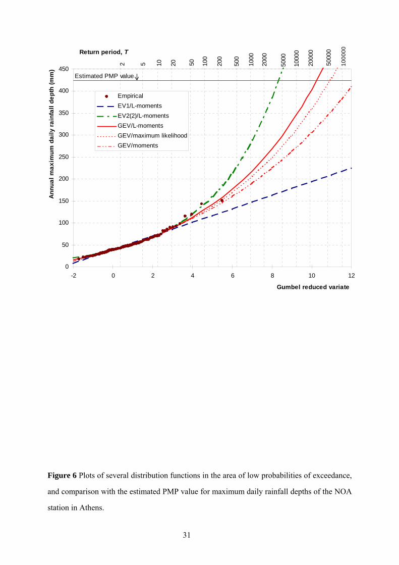
To acquire an idea of the implications of an improper adoption of the EV1 distribution,

we have re-plotted this distribution, along with the other distributions discussed above, in

Figure 6, where we have given emphasis to the right tail of the distribution, for probabilities

of exceedance less than 1/200. Clearly, the EV1 distribution, even though estimated from the

complete 136-year record, underestimates seriously the maximum rainfall for small

probabilities of exceedance. For instance, at the return period 10 000 years the EV1

distribution results in a value of rainfall depth half that obtained by the GEV distribution. We

13

note that 10 000 years is not an unusual return period for the design of major flood protection

works; for example most dam spillways in Greece were designed adopting this value.

We should emphasise that doubts about the adequacy of the EV1 distribution have been

expressed by others, as well. For example, Wilks (1993) notes that EV1 often underestimates

the largest extreme rainfall amounts and suggests an update and revision of the Technical

Paper 40 (Hershfield, 1961b), a widely used climatological atlas of United States that was

compiled fitting EV1 distributions to annual extreme rainfall data.

To complete the above discussion, we note that, if the GEV distribution must replace

the EV1 distribution in typical applications involving small sample sizes, the three parameters

of the former may be a drawback, given the well known disability of reliable parameter

estimation of three-parameter distributions. The solution to this problem can be the so-called

“substitution of space for time” (National Research Council, 1988), that is, the incorporation

in the analysis of information from other rainfall data sets from other locations in the same

region. In this respect, the analysis and results of the present work may be useful for

estimating probabilities of extreme rainfall in other parts of the country.

6. Comparison with probable maximum precipitation

The discussion in section 5 showed that a subset of the available 136-year data series may

bias seriously our knowledge of the distribution function. Besides, the distribution function

obtained by the complete 136-year series, apparently, cannot be the true population

distribution (136 years are still too low to determine the true population distribution). Thus,

the extrapolation of the GEV distribution obtained in section 4 to probabilities of exceedance

such as 1/1000, 1/10 000, or even less may lead to inaccurate results. This is a consequence of

the so-called “Myth of the Tails” (Wileeke, 1980), which reads “Statistical distributions

applied to hydrometeorological events that fit through the range of observed data are

applicable in the tails” and reminds us that the tails of distributions are highly uncertain (see

also Dooge, 1986).

Therefore, as another quantification of an extremely high rainfall magnitude we

estimated the daily probable maximum precipitation (PMP) in Athens, based on the available

14

annual series of maximum rainfall depths. More specifically, we used the so-called statistical

estimation of PMP as developed by Hershfield (1961a, 1965) and standardised by the World

Meteorological Organization (1986). The method estimates the rainfall depth hm of the

probable maximum precipitation of duration d by the formula

hm = h– + km sH (6)

where h– and sH are the sample mean and standard deviation, respectively, of maximum

rainfall depth of duration d, and km is a frequency factor given by an empirical nomograph as

a function of d and h–. This nomograph can be approximated by the simple analytical equation

(Koutsoyiannis and Xanthopoulos, 1997, p.160)

km = 20 – 8.6 ln ⎝⎜⎛

⎠⎟⎞h

–-

130 + 1 ⎝⎜⎛

⎠⎟⎞ 24

d

0.4

(7)

The method incorporates some adjustments of mean and standard deviation for sample size

and maximum observed event (World Meteorological Organization, 1986, pp. 97-107).

The application of the method to the data of this study (Table 1) with all adjustment

factors equal to one, due to the large sample size, results in km = 17.20 and a PMP value 424.1

mm for daily rainfall. This PMP value when considered from a probabilistic viewpoint can be

assigned a specific return period depending on the particular distribution function. In Table 3

we present the values of return period corresponding to rainfall depth of 424.1 mm for the

different distribution functions examined in this study. We observe that the results exhibit a

huge variability as the values vary from 4.2 thousand years for the EV2(2) distribution to 64

billion years for the EV1 distribution (see also Figure 6). To have an empirical idea about

what the true value of the return period might be, we recall that the method of Hershfield

(1961a) was based on the analysis of m = 95 000 station-years of data. That means that the

empirical probability corresponding to km (and, consequently, to hm) is of the order of p =

1 / m ≈ 10−5 and the return period is of the order of 105 years. Indeed, this is the order of

magnitude of the return period when this is estimated by the GEV distribution, the estimate

with the closest agreement being that obtained by the method of maximum likelihood. An

15

upper 99% confidence limit for p is p΄ = p + 2.58 [p (1 – p) / m]0.5 = 3.7 × 10–5 which

corresponds to a return period of 27 000 years. This suggests that the estimate of the method

of L-moments (28 000 years) is also consistent with the results of the Hershfield’s PMP

method, when the latter is considered from a probabilistic point of view.

This investigation provides another empirical indication that the GEV distribution

performs well in the case study examined, whereas the EV1 and EV2(2) distributions do not.

7. Estimation of intensity-frequency-duration curves

After the thorough investigation of the available extreme rainfall record and the results found,

some of which may have wider applicability, we must now return to the problem brought up

in section 1, i.e., the derivation of intensity-frequency-duration curves for Athens, applicable

for high return periods. To this aim, we follow a newly developed mathematical framework

for constructing idf curves, whose details are given elsewhere (Koutsoyiannis et al., 1998).

The results of the previous sections can be utilised to determine a(T) in equation (1). At

this time we do not have available maximum rainfall data of the NOA station for durations

shorter than daily, so we have adopted the function b(d) of a nearby rain-recording station,

namely Helliniko, that is (Koutsoyiannis et al., 1998)

b(d) = (d + 0.189) 0.796 (d in h) (8)

We note that this function was derived by making no hypothesis about the distribution

function of rainfall depth or intensity using a non-parametric statistical technique

(Koutsoyiannis et al., 1998) and the numerical coefficients (0.189 and 0.796) were found to

be reasonably constant over a wider geographical area (Koutsoyiannis et al., 1998; Kozonis,

1995).

Solving (4) for x ≡ h(d, T), and replacing FX by 1 – 1 / T, we get

h(24, T) = λ

⎩⎪⎨⎪⎧

⎭⎪⎬⎪⎫⎣⎢

⎡⎦⎥⎤−ln ⎝⎜

⎛⎠⎟⎞1 −

1T

–κ

– 1

κ

+ ψ (9)

16

Adopting the parameter values of the method of L-moments, which result in safer (higher)

values of rainfall depth in the upper tail of the distribution (Figure 6) and replacing them in

(9) we get

h(24, T) = 68.32 ⎩⎪⎨⎪⎧

⎭⎪⎬⎪⎫

⎣⎢⎡

⎦⎥⎤−ln ⎝⎜

⎛⎠⎟⎞1 −

1T

–0.185

– 0.45 (10)

Combining (1), (8), and (10) and solving for i(d, T) := h(d, T) /d we obtain the idf relationship

i(d, T) = 35.95

⎩⎪⎨⎪⎧

⎭⎪⎬⎪⎫

⎣⎢⎡

⎦⎥⎤−ln ⎝⎜

⎛⎠⎟⎞1 −

1T

–0.185

– 0.45

(d + 0.189) 0.796 (11)

For large return periods, e.g., T ≥ 50 we can write ln [1 − (1/T)] = −(1/T) − (1/T)2 − L ≈

−(1/T) which simplifies (11). Furthermore, (11) needs an adjustment to account for the fact

that the daily rainfall depth is a fixed-interval rainfall amount. Using the adjusting factor of

the bibliography (e.g., Linsley et al., 1975, p. 357), which is 1.13, and making the

simplification we finally obtain

i(d, T) = 40.6 (T 0.185 – 0.45)

(d + 0.189) 0.796 (i in mm/h, t in h) (12)

The simplified and adjusted equation (12) is also valid for small return periods if we replace

the return period T for the annual series with the return period T ΄ for the series over threshold

(or partial duration series). Indeed, in that case we have (see, e.g., Raudkivi, 1979, p. 411)

–ln (1 – 1 / T) = 1/T ΄ (13)

so that (11) again results in (12) with T ΄ substituted for T.

A plot of idf relationship (12) is given in Figure 7 along with a comparison with the

most widespread of earlier relationships, which were constructed using empirical techniques

(Dallas, 1968, Memos, 1980). The large departures among the different sets of curves are

apparent in this figure, especially for large return periods T = 1000 - 10 000 years. These

departures are explained by the smaller sample sizes and the empirical techniques used to

17

derive the earlier relationships. Due to the longer record used in the present study and the

more thorough study and the refined and consistent methodology, it is expected that the

relationship (12) is more reliable than those developed in the past.

8. Conclusions

The analysis of the longest record of annual maximum daily rainfall in Greece, i.e. the 136-

year series of the NOA station in Athens, results in useful findings both for prediction of

intense rainfall in Athens, where currently major flood protection works are under way, and

for investigating more generalised issues like the adequacy of extreme value distributions for

extreme rainfall analysis, and the effect of sample size on design rainfall inferences.

Statistical exploration and tests based on this long record indicate no statistically

significant climatic changes in extreme rainfall during the last 136 years. Furthermore,

statistical analysis shows that the conventionally employed EV1 distribution is inappropriate

for the examined record (especially in its upper tail), whereas this distribution would seem as

an appropriate model if fewer years of measurements were available (i.e., part of this sample

were used). Simulation experiments showed that, when the record length is small, the

misleading appearance of the EV1 distribution as an appropriate one, is not a peculiarity of

the examined record but a generalised statistical effect. On the contrary, the General Extreme

Value (GEV) distribution appears to be suitable for the examined series and its predictions for

large return periods agree with the estimate of probable maximum precipitation obtained by

the statistical (Hershfield’s) method, when the latter is considered from a probabilistic point

of view. Thus, the results of the analysis of this record agree with a recently (and

internationally) expressed scepticism about the EV1 distribution which tends to underestimate

the largest extreme rainfall amounts. It is demonstrated that the underestimation is quite

substantial (e.g. 1:2) for large return periods and this fact must be considered as a warning

against the widespread adoption of the EV1 distribution for rainfall extremes.

Although a 136-year record is still too short to accurately determine the upper tail of the

distribution function of maximum rainfall, it is quite longer than typical samples available for

hydrologic applications such as the construction of intensity-duration-frequency relationships.

18

Thus, this record provides a clearer view of such relationships for large return periods, and

based on a newly developed methodology, the fitted GEV distribution is directly utilised for

establishing their mathematical expressions.

Acknowledgements

The authors are grateful to the National Observatory of Athens and the Academy of Athens -

Research Centre of Atmospheric Physics and Climatology for their kind permission of access

to some of the oldest files and Annual Climatological Bulletins. They also thank A. Paliatsos

of the Technological Educational Institute of Pireas, Greece, for providing useful information

for the years 1890-1930. The constructive comments of an anonymous reviewer are gratefully

appreciated.

19

References

Chowdhury, J. U., J. R. Stedinger, and L.-H. Lu, Goodness-of-fit tests for regional

generalized extreme value flood distributions, Water Resour. Res., 27(7), 1765-1776,

1991.

Dallas, S., Study of the rehabilitation of the Kifissos River (in Greek), Sewage Organisation

of Athens, 1968.

Deas, N., Geographical distribution on intense rainfall in the Sterea Hellas area, Diploma

thesis (in Greek), National Technical University, Athens, 1994.

Dooge, J. C. I., Looking for hydrologic laws, Water Resour. Res., 22(9) pp. 46S-58S, 1986.

Hershfield, D. M., Estimating the probable maximum precipitation, Proc. ASCE, J. Hydraul.

Div., 87(HY5), 99-106, 1961a.

Hershfield, D. M., Rainfall Frequency Atlas of the United States, U.S. Weather Bur. Tech.

Pap. TP-40, Washington, D.C., 1961b.

Hershfield, D. M., Method for estimating probable maximum precipitation, J. American

Waterworks Association, 57, 965-972, 1965.

Hirsch, R. M., D. R. Helsel, T. A. Cohn, and E. J. Gilroy, Statistical analysis of hydrologic

data, in Handbook of Hydrology, edited by D. R. Maidment, McGraw-Hill, 1993.

Hosking, J. R. M., L-moments: Analysis and estimation of distributions using linear

combinations of order statistics, J. R. Stat. Soc., Ser. B, 52, 105-124, 1990.

Hosking, J. R. M., J. R. Wallis and E. F. Wood, Estimation of the generalized extreme value

distribution by the method of probability weighted moments, Technometrics, 27(3),

251-261, 1985.

Hydrauliki, Study of the sanitary and storm sewer networks of Acharnes, Ano Liosia,

Kamatero and Zefiri, Engineering Report, 204 pp. (in Greek), Sewage Organisation of

Athens, 1980.

Katsoulis, B. D., and H. D. Kambetzidis, Analysis of the long-term precipitation series at

Athens, Greece, Climatic change, 14, 263-290, 1989.

Kottegoda, N. T., Stochastic Water Resources Technology, Macmillan Press, London, 1980.

20

Koukis, G. C., and D. Koutsoyiannis, Greece, in Geomorphological Hazards of Europe,

edited by C. and C. Embleton, Elsevier, pp. 215-241, Amsterdam, 1997.

Koutsoyiannis, D., D. Kozonis and A. Manetas, A comprehensive study of rainfall intensity-

duration-frequency relationship, J. of Hydrol., 206, 118-135, 1998.

Koutsoyiannis, D., and Th. Xanthopoulos, Engineering Hydrology, 412 pp. (in Greek),

National Technical University, Athens, 1997.

Kozonis, D., Construction of idf curves from incomplete data sets, Application to the Sterea

Hellas area, Diploma thesis (in Greek), National Technical University, Athens, 1995.

Linsley, R. K. Jr., M. A. Kohler and J. L. H. Paulus, Hydrology for Engineers, McGraw-Hill,

Tokyo, 2nd edition, 1975.

Mariolopoulos, H., The Climate of Greece, National Observatory of Athens, 280 pp. (in

Greek), 1938.

Memos, C., Intensity-duration-frequency curves for large intensities, Proc. 2nd Greek

seminar on hydrology, 57-65 (in Greek), Ministry of Coordination, Athens, 1980.

National Research Council, Estimating Probabilities of Extreme Floods: Methods and

Recommended Research, National Academy Press, Washington, D.C., 1988.

Nicolaidou, M. and E. Hadjichristou, Recording and assessment of flood damages in Greece

and Cyprus, Diploma thesis (in Greek), National Technical University of Athens,1995.

Xanthopoulos, Th., D. Christoulas, M. Mimikou, D. Koutsoyiannis and M. Aftias, A strategy

for the problem of floods in Athens, Proc. of the Workshop for the Flood Protection of

Athens (in Greek), Technical Chamber of Greece, Athens, 1995.

Raudkivi, A. J., Hydrology, An Advanced Introduction to Hydrological Processes and

Modelling, Pergamon Press, Oxford, 1979.

Stedinger, J. R., R. M. Vogel, and E. Foufoula-Georgiou, Frequency analysis of extreme

events, Chapter 18 in Handbook of Hydrology, edited by D. R. Maidment, McGraw-

Hill, 1993.

Wilks, D. S., Comparison of three-parameter probability distributions for representing annual

extreme and partial duration precipitation series, Water Resour. Res., 29(10), 3543-

3549, 1993.

21

Willeke, G. E., Myths and uses of hydrometeorology in forecasting, in Proceedings of March

1979 Engineering Foundation Conference on Improved Hydrological Forecasting –

Why and How, pp. 117-124, American Society of Civil Engineers, New York, 1980.

World Meteorological Organization (WMO), Manual for Estimation of Probable Maximum

Precipitation, Operational Hydrology Report 1, 2nd edition, Publication 332, World

Meteorological Organization, Geneva, 1986.

Zerefos, C. S, G. B. Kosmas, C. C. Repapis, and J. D. Zambakas, Time series analysis of rain

at Athens National Observatory during the century 1871-1970, Report (in Greek),

National Observatory of Athens, 39 pp., 1977.

22

List of Tables

Table 1 Statistics of the sample of annual maximum daily rainfall depths (in mm) of the NOA

station in Athens.

Table 2 Parameter values of various distribution functions fitted to the sample of annual

maximum daily rainfall depths (in mm) of the NOA station in Athens.

Table 3 Return period of the PMP value as estimated using the various distribution functions

fitted to the sample of annual maximum daily rainfall depths of the NOA station in Athens.

23

Table 1 Statistics of the sample of annual maximum daily rainfall depths (in mm) of the NOA

station in Athens.

Statistic Value

Sample size 136

Maximum value 150.8

Minimum value 17.2

Mean 47.9

Median 42.5

Standard deviation 21.7

Interquartile range 19.7

Coefficient of variation 0.454

Coefficient of skewness 2.13

Coefficient of kurtosis 6.30

L-coefficient of variation 0.224

L-coefficient of skewness 0.294

L-coefficient of kurtosis 0.242

Table 2 Parameter values of various distribution functions fitted to the sample of annual

maximum daily rainfall depths (in mm) of the NOA station in Athens.

Distribution Fitting Transformation Parameter values

of variable method of variable κ λ ψ

EV1 Moments None (0) 16.89 2.26

EV1 L-moments None (0) 15.48 2.51

EV2(2) L-moments None 0.292 10.87 (3.43)

GEV Moments None 0.118 14.07 2.69

GEV L-moments None 0.185 12.64 2.99

GEV Max. likelihood None 0.161 12.93 2.94

GEV L-moments Logarithmic –0.136 0.345 10.51

24

Table 3 Return period of the PMP value as estimated using the various distribution functions

fitted to the sample of annual maximum daily rainfall depths of the NOA station in Athens.

Distribution of variable EV1 EV1 EV2(2) GEV GEV GEV

Fitting Method Moments L-moments L-moments Moments L-moments Max. likelihood

Return period of PMP 8.4 × 109 64 × 109 4 200 210 000 28 000 56 000

25

List of Figures

Figure 1 Time series of the annual maximum daily rainfall depth at the NOA station.

Figure 2 Box plots of the complete series of annual maximum rainfall depths and the four

sub-series each corresponding to one quarter of the record length.

Figure 3 Probability of occurrence of each year’s annual maximum rainfall in each of the

twelve months, as estimated from the complete series of annual maximum rainfall depths and

the four sub-series each corresponding to one quarter of the record length.

Figure 4 EV1, EV2(2), and GEV distributions fitted to the sample of annual maximum daily

rainfall depths by the method of L-moments, in comparison with the empirical distribution

estimated using Gringorten plotting positions.

Figure 5 Comparison of the distribution function of the complete series of annual maximum

rainfall depths (136 years) and the fourth sub-series corresponding to one quarter of the record

length (last 34 years).

Figure 6 Plots of several distribution functions in the area of low probabilities of exceedance,

and comparison with the estimated PMP value for maximum daily rainfall depths of the NOA

station in Athens.

Figure 7 Comparison of intensity-frequency duration curves for Athens derived in this study

(solid curves; eqn. (12)) with earlier empirical idf curves of the same region.

0

20

40

60

80

100

120

140

160

1860 1870 1880 1890 1900 1910 1920 1930 1940 1950 1960 1970 1980 1990

Ann

ual m

axim

um d

aily

rain

fall

dept

h (m

m)

Annual value21-year moving average

Figure 1 Time series of the annual maximum daily rainfall depth at the NOA station.

26

0

20

40

60

80

100

120

140

160

Ann

ual m

axim

um d

aily

rain

fall

(mm

)

Completerecord

Firstquarter

Secondquarter

Thirdquarter

Fourthquarter

136 years 34 years 34 years 34 years 34 years

Figure 2 Box plots of the complete series of annual maximum rainfall depths and the four

sub-series each corresponding to one quarter of the record length.

27

0%

5%

10%

15%

20%

25%

30%

35%

1 2 3 4 5 6 7 8 9 10 11 1

Month

Prob

abili

ty o

f occ

uren

ce

of a

nnua

l max

imum

rain

fall

2

Complete record (136 years)95% confidence limitsFirst quarterSecond quarterThird quarterFourth quarter

Figure 3 Probability of occurrence of each year’s annual maximum rainfall in each of the

twelve months, as estimated from the complete series of annual maximum rainfall depths and

the four sub-series each corresponding to one quarter of the record length.

28

0

20

40

60

80

100

120

140

160

180

200

-2 -1 0 1 2 3 4 5

Gumbel reduced variate

Annu

al m

axim

um d

aily

rain

fall

dept

h (m

m)

6

EmpiricalEV1

EV2(2)GEV

T = 2 5 10 20 50 100 200

Figure 4 EV1, EV2(2), and GEV distributions fitted to the sample of annual maximum daily

rainfall depths by the method of L-moments, in comparison with the empirical distribution

estimated using Gringorten plotting positions.

29

0

20

40

60

80

100

120

140

160

-2 -1 0 1 2 3 4 5 6

Gumbel reduced variate

Ann

ual m

axim

um d

aily

rai

nfal

l dep

th (m

m)

Empirical/All 136 yearsEmpirical/Last 34 yearsGEV/All 136 years

EV1/All 136 yearsEV1/Last 34 years

T = 2 5 10 20 50 100 200

Figure 5 Comparison of the distribution function of the complete series of annual maximum

rainfall depths (136 years) and the fourth sub-series corresponding to one quarter of the record

length (last 34 years).

30

0

50

100

150

200

250

300

350

400

450

-2 0 2 4 6 8 10 12

Gumbel reduced variate

Ann

ual m

axim

um d

aily

rai

nfal

l dep

th (m

m)

EmpiricalEV1/L-momentsEV2(2)/L-momentsGEV/L-momentsGEV/maximum likelihoodGEV/moments

Return period, T

5 10 20 50 100

200

500

1000

2000

5000

1000

0

2000

0

5000

0

1000

00

2

Estimated PMP value

Figure 6 Plots of several distribution functions in the area of low probabilities of exceedance,

and comparison with the estimated PMP value for maximum daily rainfall depths of the NOA

station in Athens.

31

T = 10

T = 100

T = 1000

T = 10 000

1

10

100

1000

0.1 1 10 100

Dura tion, d (h)

Rai

nfal

l int

ensi

ty, i

(mm

/h)

⎪⎪⎩

⎪⎪⎨

⎧

>

≤=

− mm /h 3013.8

mm/h 308.12

(1980) Memos to due onModificati

016.05.02/1

3/2

3/1

iedT

id

T

ii

796.0

185.0

)189.0(

)45.0(6.40study) (this (12) Equation

+

−=

d

Ti

3/2

3/18.12(1968) Dallas to due Equation

d

Ti =

Figure 7 Comparison of intensity-frequency duration curves for Athens derived in this study

(solid curves; eqn. (12)) with earlier empirical idf curves of the same region.

32