Analysis for Strategic Planning Applied to Ethanol and ... · Applied to Ethanol and Distillers’...

2013 International Food and Agribusiness Management Association (IFAMA). All rights reserved

37

International Food and Agribusiness Management Review Volume 16, Special Issue 3, 2013

Analysis for Strategic Planning

Applied to Ethanol and Distillers’ Grain

Dennis M. Conley

Professor and Director, Graduate Program in Agribusiness, Department of Agricultural Economics University of Nebraska – Lincoln, Lincoln, Nebraska, 68583-0922, USA

Abstract While traditional economic analysis is a look back on past events and relationships, the motivation for strategic planning is to look forward. An example, based on the ethanol and distillers’ grain industry, illustrates the kind of analysis that can used for strategic planning by agribusiness firms and non-governmental organizations. It is expected that the current U.S. monetary policy of expanding the money supply, a Renewable Fuel Standard mandating 15 billion gallons of ethanol, and a growing export market for distillers' grains could potentially result in the future production of ethanol and distillers' grain that would be well above a normal trend. The corresponding derived demand for corn, relative to the normal increases in supply, would significantly affect the price levels for corn. Keywords: strategic planning, ethanol, distillers’ grain, renewable fuels, exchange rates, corn, prices, scenarios

Corresponding author: Tel: + 1. 402.472.2034 Email: D. Conley: [email protected]

Conley Volume 16 Issue 3, 2013

2013 International Food and Agribusiness Management Association (IFAMA). All rights reserved.

38

Introduction When an agribusiness engages in strategic planning it begins a process of identifying goals and objectives for the future; determining how to accomplish the same; and to complete the process - estimating the resources needed. The process is both qualitative—what are the likely scenarios, and quantitative—what are the numerical measures of outcomes. Taking the process from a conceptual framework to specific application requires an analysis of current conditions and future scenarios which serve as boundaries for the goals and objectives. When an agribusiness retreats to engage in the process, senior management selects a cadre of managers who have experience with a collection of industry and public policy events over time. Those experiences result in the learning and internalizing of conditions that affect the agribusiness. It is a valuable and irreplaceable wisdom that contributes to a manager's historical perspective. When analyzing conditions in U.S. agriculture, there were a few historical periods when a collection of events brought about significant structural changes for row crop farmers, livestock producers and the agribusinesses that serve them. One of those periods was 1971-72. In August of 1971, President Richard Nixon unilaterally cancelled the direct convertibility of the U.S. dollar to gold, in effect going off the long-standing gold standard of $35 an ounce. The U.S. dollar was devalued by 7 percent. In April 1972, the new Secretary of Agriculture, Earl Butz, led a delegation of U.S. government officials to Moscow, the Soviet Union, to offer a line of credit for the purchase of U.S. grain over a three year period. Russian grain crops had not come through the winter very well and might be in short supply. With large surpluses of wheat, corn and soybeans in the U.S., the delegation was prospecting to see if the Soviet Union was interested in buying. Initially, they did not think the terms of the deal were favorable and declined to do anything. A few months later, on June 25, 1972 a crop report came out for the production estimates in the Soviet Union. This may have been a tipping point (Gladwell 2000). Within a few days the U.S. State Department received an urgent request to issue visas for Soviet officials to come to the U.S. ostensibly with the intent on buying grain (Morgan 139-160). In July and August 1972, the United States sold the Soviet Union about 440 million bushels of wheat, more than the total U.S. commercial wheat exports for the year beginning in July 1971. The sales were equivalent to 30 percent of average annual U.S. wheat production during the previous five years and more than 80 percent of the wheat used for domestic food during that period. Immediately following the sales announcements, the domestic price of wheat began to rise, and within a few months the prices of feed and food grain, soybeans, and livestock turned upward (Luttrell, p. 2). See Figure 1. The Soviet Union came to the U.S. after 1972 and continued to purchase grain sustaining the higher price levels. These events and changes also led to higher price volatility as shown by the wider range of prices in the figure. The U.S. agriculture economy became less supply-managed by the government and much more export led. As a side note, international agricultural trade and the use of futures markets to manage price risk emerged as important areas of study in academia.



39

Figure 1. U.S. Price of Wheat, 1950-2006. In more recent times, another example provides a historical perspective for use in strategic planning. Again, a collection of events during the years 2002-06 brought about structural changes for row crop farmers, livestock producers and the agribusinesses that serve them. This time the changes were triggered by the use of ethanol. Ethanol had been around for a long time. Henry Ford designed the Model T in 1908 to run on ethanol, gasoline or both. But the oil industry provided less expansive gasoline and ethanol didn't become part of the motor gasoline supplied until decades later. On December 17, 1963 President Lyndon B. Johnson signed the Clear Air Act into law. It was designed to control air pollution at a national level and required the Environmental Protection Agency (EPA) to develop and enforce regulations protecting the public from airborne contaminants known to be hazardous to human health. In 1992, amendments to the Clear Air Act required reduction of carbon monoxide emissions, primarily from vehicles. This led to the widespread use of methyl tertiary butyl ether (MTBE) as an oxygenate additive to gasoline. However, once it was discovered that MTBE contaminated groundwater, the additive was banned in almost 20 states by 2006. Suppliers were concerned about potential litigation stemming from a 2005 court decision denying legal protection for MTBE. This was likely a tipping point for the ethanol industry because ethanol became the oxygenate of choice for gasoline. Concurrent federal legislation contributed to the rapid growth in ethanol consumption with the goals of reducing oil consumption and dependence on foreign sources. The Energy Policy Act of 2005 required the use of 7.5 billion gallons of renewable fuel by 2012, and the Energy Independence and Security Act of 2007 raised the requirement to 36 billion gallons by 2022. Of this requirement, 15 billion gallons are to be ethanol by 2015. The following figure shows the

http://en.wikipedia.org/wiki/Methyl_tert-butyl_ether



40

decline in MTBE production starting in 2002 and the corresponding increase in ethanol production in response to the above changes.

0

50

100

150

200

250

300

350

400

450

1998 1999 2000 2001 2002 2003 2004 2005 2006 2007

1,00

0 ba

rrel

s per

day

Production of MTBE and Ethanol

MTBE

Ethanol

Figure 2. Production of MTBE and Ethanol, 1998-2007.

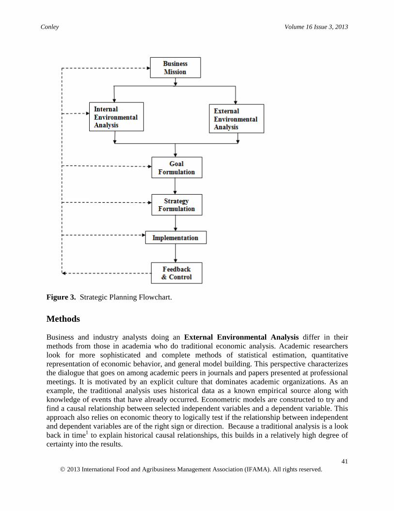
Strategic Planning The two examples from agriculture bring us to the question, "When doing strategic planning is it useful to do a scan of historical events where each one by itself may not make a difference, but taken collectively, can result in structural change? The literature on strategic planning is wide and deep and the flowchart in Figure 3 provides a general model. The Business Mission is a statement about the purpose of the business and what it wants to accomplish over a long-run time period. The Internal Environmental Analysis is an assessment of those factors internal to the organization that management and employees have some control over and can change, as needed. The boxes of Goal Formulation, Strategy Formulation, Implementation, and Feedback & Control are familiar and self-explanatory. The External Environmental Analysis is an assessment of those factors outside the organization that managers have very little or no controls over, yet could impact the business. Industry and public policy events are prime examples. The focus of the research illustrated in this article is centered on this box. It is about an approach, or a way of watching for events, and a collection of events, that contributes to an external environmental analysis.



41

Figure 3. Strategic Planning Flowchart.

Methods Business and industry analysts doing an External Environmental Analysis differ in their methods from those in academia who do traditional economic analysis. Academic researchers look for more sophisticated and complete methods of statistical estimation, quantitative representation of economic behavior, and general model building. This perspective characterizes the dialogue that goes on among academic peers in journals and papers presented at professional meetings. It is motivated by an explicit culture that dominates academic organizations. As an example, the traditional analysis uses historical data as a known empirical source along with knowledge of events that have already occurred. Econometric models are constructed to try and find a causal relationship between selected independent variables and a dependent variable. This approach also relies on economic theory to logically test if the relationship between independent and dependent variables are of the right sign or direction. Because a traditional analysis is a look back in time1 to explain historical causal relationships, this builds in a relatively high degree of certainty into the results.



42

In strategic planning the challenge is to look forward and do an analysis that describes probable scenarios. Unlike the conditions of certainty in the past, strategic planning is an attempt to manage or mitigate the uncertain conditions of the future. In so doing the industry analyst needs to consider the knowledge and experiences acquired by managers and boards of directors, and to use methods that are credible to them. These methods are generally structured differently than the traditional analysis seen in academia. Agribusiness managers and boards of directors acquire knowledge of their industry in a characteristically human manner - they talk and listen to those people who they think have insights into the future. Common behavior is to attend industry association events and conferences (such as the one hosted by the International Food and Agribusiness Management Association) and interact with their peers seeking their opinions, and giving their own, to gain insights into changing environmental conditions. If time permits they may read trade publications. One method that industry analysts regularly use is called the "balance sheet" approach. It includes data describing the historical supply and disappearance of a commodity and corresponding prices or price ranges. The World Agricultural Supply and Demand Estimates (WASDE) reports published by the U.S. Department of Agriculture (USDA) are the most notable commodity balance sheets. The reports are read closely by those in agriculture and agribusiness throughout the world. They give historical data in a balance sheet and also include short-run projections by USDA analysts on supply and disappearance of commodities along with estimates on a price range. The balance sheet approach is more open-ended than traditional analysis and gives the analyst the flexibility to craft probable scenarios based on the current environment and expectations about the future. This approach to looking forward appeals to managers because they know how to interpret a commodity balance sheet, such as the WASDE, and from it can follow the formulation of probable scenarios. In contrast, traditional economic analysis with structured models is usually not readily understood by managers, or a board of directors. To them there is a "black box" effect where something goes in, is processed, and the results come out. Because they cannot follow or track what happens and why, they are inclined to not trust the results. Objective Based on an astute awareness of external environmental factors such as proposed government policy, consumer tastes and preferences, emerging technology, etc., the question is, "How can this information be used to craft future business scenarios that have a reasonable probability of occurrence?" Related to this question is the challenge to explain to industry managers and boards of directors the economic behavior and outcomes in a way that is clear and they can accept with ______________________________________________________________________________ 1 Even though the traditional economic analysis is a look back and based on certainty, it is by no means useless. It helps the industry analyst identify critical variables worth watching in the current environment, and gives some relative weight to those variables. When a causal relationship is empirically confirmed with historical data and econometric models, the analyst can make use of it in developing future scenarios. Indeed, the statistically significant and logically correct variables provide a good starting point for anticipating the events, or conditions, that may make a big difference - that is, may lead to structural change.



43

some degree of confidence. Derivation of future behavior and outcomes needs to be transparent and resonate with their historical experiences. The objective of this article is to illustrate, by example for both academic and industry audiences, the kind of analysis needed for strategic planning. The following example shows how critical knowledge of external environmental factors and a historical perspective of events can be used to develop probable outlook scenarios. Problem Statement The U.S. ethanol industry has grown from a production level of 1.6 billion gallons in 2000 to a high of 13.7 billion in 2011 - over an 8 fold increase in twelve years. Based on a Renewable Fuel Standard that mandates 15 billion gallons of ethanol from corn by 2015, some experts think that will be the upper limit in the long term. However, if history provides any lessons the increasing trend suggests future ethanol production could reach the mandate before the 2015 deadline. That history signals production levels being determined by market conditions and not mandates. While the rapid growth in ethanol production and consumption in recent years has focused the industry and public's attention on ethanol's contribution to the fuel supply, distillers' grain early on was considered only a by-product of the production process to be disposed of at market clearing prices. The nutritional value is higher than for corn as a feed grain, yet the price on distillers' grain was discounted to that of corn. Over time livestock feeders adopted distillers' grain in place of corn and the price now reflects a small premium to that of corn. Not only have U.S. feeders adopted distillers' grain but so have their counterparts in foreign countries. The developing export situation leads to questions by agribusiness managers, livestock producers and industry representatives about the future impacts on the ethanol industry and more fundamentally on the price of corn. What could be the projected levels of distillers' grain exports over the next five years? What would be the associated levels of ethanol production needed to satisfy the domestic and export demand? What impact would higher levels of ethanol production, derived from higher export demand for distillers' grain, have on the prices of corn over the next five years? Scenario Objectives In response to the preceding questions, the objectives for developing scenarios are to:

a) Project three levels of ethanol production out to 2017 based on the Renewable Fuel Standard and Environmental Protection Agency (EPA) regulations.

b) Establish two scenarios on distillers' grain exports out to 2017 based on projected

exchange rates related to U.S. monetary policy.

c) Estimate the historical relationship of the price of corn to ending stocks in the U.S. from 1989 through 2012.



44

From the above, derive results that project price outlook scenarios for corn out to 2017. Objective 1 In December 2007 the U.S. Congress passed the Energy Independence and Security Act which was subsequently signed into law by President Bush. The Act mandated a Renewable Fuel Standard (RFS) of 36 billion gallons of biofuels from multiple sources by the year 2022. The target mandate for corn as a source was 15 billion gallons by 2015. In October 2010, the U.S. Environmental Protection Agency (EPA) expanded the permissible volume of ethanol in a gallon of gasoline from 10 percent (E10) to 15 percent (E15) for motor vehicles manufactured since 2007. The EPA did additional testing to determine if E15 can be used in vehicles manufactured in the 2001 - 2006 time period and subsequently gave approval. Under these conditions, estimates are that more than 50 percent of the U.S. vehicle fleet could use E15. One motivation for E15 was to move the "blend wall" confronting the ethanol industry because of the recent rapid growth in production. With the Renewable Fuels Standards mandated at 15 billion gallons of ethanol from corn, but motor fuel consumption projected to only reach 140 billion gallons by 2015, the 10 percent blend, or 14 billion gallons of ethanol, would be below the mandate - hence the "blend wall". See Figure 4. Raising the blend level to 15 percent would allow ethanol production to reach and even exceed the mandated 15 billion gallons in the near term. At the higher level, the trend increase shows that the blend wall would not become constraining until around 2017, if at all.

Figure 4. Ethanol Production from Corn, 200-2011, and Projected to 2017.



45

Objective 2 U.S. monetary policy is implemented by the U.S. Federal Reserve System (FED). Due to the severe recession that started in 2008, the current policy has a macroeconomic focus intended to reduce uncertainty in the financial sector by guaranteeing liquidity and reducing unemployment that was around 8 percent – a level considered too high by about double. The policy was implemented using a program of Quantitative Easing that increased the monetary base from $831 billion in 2008 to $2.742 trillion by January 2013 - an increase of $1.9 trillion to more than triple the base in 2008. See Figure 5.

Figure 5. Federal Reserve Board of Governors Monetary Base, 2000-2013.

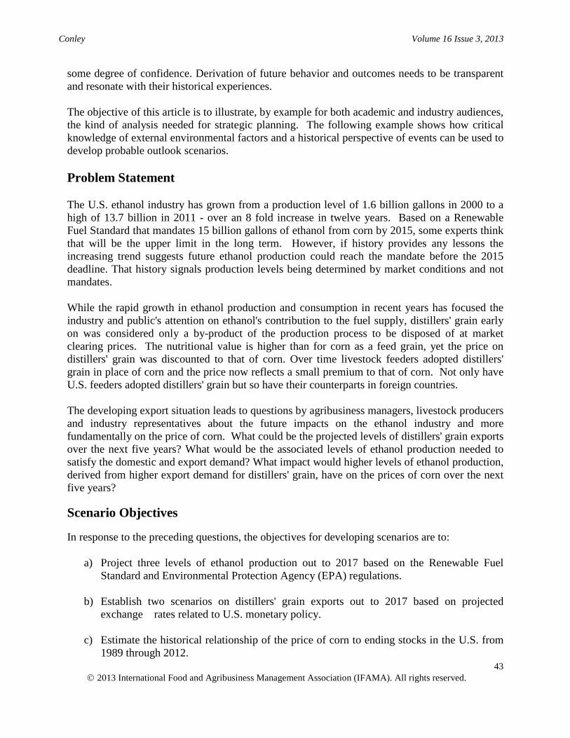
The ongoing increases in money supply have kept long term interest rates at record low levels, and the FED declared it will keep interest rates low for the next few years. This also affects the value of the dollar as a currency used in international trade. The trade weighted exchange rate for corn is shown in the following figure. (Distillers' grains are a direct feed substitute for corn.) The exchange rate index has been declining for the past eleven years which made U.S. exports of corn, and similarly distillers' dried grains (DDGs), less expensive to foreign buyers. Extending out to 2017, the exchange rate index is projected to be 77 by the year 2017.



46

Figure 6. Trade Weighted Exchange Rate for Corn. As background information, during the years 2006-12 there emerged a significant export market for distillers’ dried grain, notably to China, Mexico and Canada. See Figure 7.

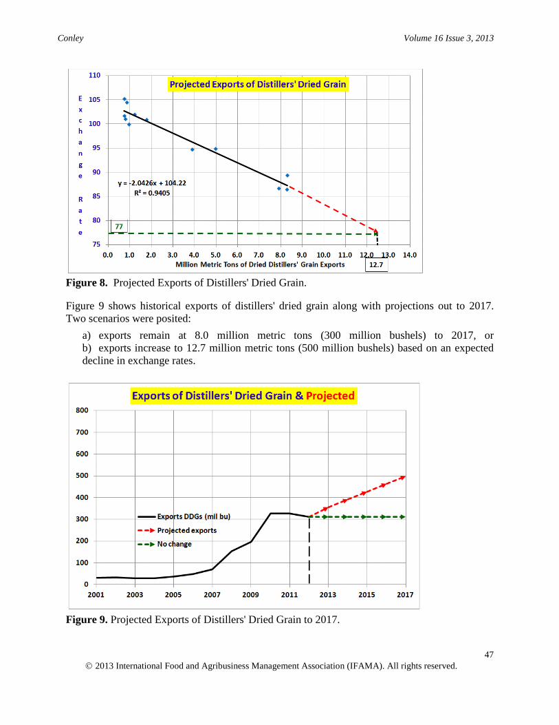
Figure 7. U.S. Exports of Distillers' Grain to Selected Countries, 2000-2012. Total exports of DDGs were plotted against the trade weighted exchange rate for corn over the past 12 years and are shown in Figure 8. In the 2011 and 2012 marketing years, exports were around 8.0 million metric tons (300 million bushels) when the exchange rate index was around 87. Applying the projected trade weighted exchange rate of 77 shown in Figure 6 out to 2017 results in estimated exports of 12.7 million metric tons (500 million bushels).



47

Figure 8. Projected Exports of Distillers' Dried Grain. Figure 9 shows historical exports of distillers' dried grain along with projections out to 2017. Two scenarios were posited:

a) exports remain at 8.0 million metric tons (300 million bushels) to 2017, or b) exports increase to 12.7 million metric tons (500 million bushels) based on an expected decline in exchange rates.

Figure 9. Projected Exports of Distillers' Dried Grain to 2017.



48

Objective 3 Data was collected on the historical and current supply and disappearance of corn from USDA's World Agricultural Supply and Demand Estimates (WASDE). The relationship of prices to ending stocks was graphed as shown in Figure 10. In the lower part to the graph for the 17 year period of 1989-2005 the relationship of the farm price to ending stocks was fairly stable. When ending stocks would range from 1.6 billion bushels up to 2.1 billion the price would be in a narrow range of $2.05 to $1.90, respectively. An easy rule of thumb to remember was that an ending stock of 2 billion bushels resulted in a price of $2.00. Ending stocks in the 0.80 to 1.5 billion bushel range would be higher and range from around $2.80 to $2.20, respectively. In the one rare year, 1995, where the ending stock was below 0.5 billion bushels, the price exceeded $3.00. In 2006 the relationship of prices to ending stocks began a structural change. The ending stock was 1.34 billion bushels but the farm price for corn ended up being $3.04. One dominant factor was the earlier mentioned ban on the use of MTBE as an oxygenate in fuel. Ethanol replaced MTBE but was in short supply at the time resulting in high prices. This caused a strong derived demand for corn and bid up its price. Another dominant factor could have been the declining value of the dollar and the favorable exchange rates for importers of corn. Exports did not decline from previous years even with the higher price of corn.

Figure 10. Farm Price for Corn versus Ending Stock, 1989-2012.



49

Scenario Results Scenario I: Attached in the Appendix is USDA's Long-Term Projections Report with Table 18 on page 66 showing marketing year supply and disappearance of corn out to 2021/22. The utilization of corn for ethanol in 2017 is projected at 5.175 billion bushels. This would yield 14.5 billion gallons of ethanol and still be under the RFS mandate of 15 billion gallons by 2015. Over the period of 2012/13 to 2017/18 ending stocks are in the 1.48 to 1.68 billion bushel range. USDA's projected prices for corn are $4.30 to $5.00 and would be about $0.50 higher than prices derived from the relationship in Figure 10 above. The lower set of projected prices, based on Figure 10, are shown in Figure 11 and would still be the 1st New Normal range. This scenario would be considered a baseline situation where economic conditions and external environmental variables are in a normal state. Events like drought or other critical events are absent. However, it is the deviation from the normal state that senior managers and board members want to know about. What are the underlying assumptions, relationships, possible changes and insights that bring about a deviation, and what are the expected outcomes? This leads us to Scenarios II and III.

Figure 11. Scenario I - Projected Farm Prices versus Ending Stocks, 2013-17. Scenario II: Also based on USDA’s long-term projections for corn out to 2017, what if ethanol production reaches 15 billion gallons and meets the RFS mandate? The higher level of ethanol production would use more of the projected supply of corn. Ending stocks would decline to the 1.15 to 1.50 billion bushel range. Based on Figure 10 projected corn prices would be $4.40 to $5.50. The prices are still in the 1st New Normal range shown in Figure 12.

1.00

2.00

3.00

4.00

5.00

6.00

7.00

8.00

9.00

0.25 0.50 0.75 1.00 1.25 1.50 1.75 2.00 2.25 2.50

$/bu

Ending Stocks billion bu

Projected Farm Price Received vs Ending Stock, Corn 2013 - 2017Based on USDA Long Term Projections

2013

2017

After 20061st New Normal

$4.00 to $6.00



50

1.00

2.00

3.00

4.00

5.00

6.00

7.00

8.00

9.00

0.25 0.50 0.75 1.00 1.25 1.50 1.75 2.00 2.25 2.50

$/bu


Projected Farm Price Received vs Ending Stock, Corn 2013 - 2017Based on 16.5 billion gallons of ethanol by 2017 & 53% higher DDG exports

2013

2017


$4.00 to $6.002013

2015

2017

2013

2015

2017

2016

After 2014 ??2nd New Normal

$6.00 to $8.00

1.00

2.00

3.00

4.00

5.00

6.00

7.00

8.00

9.00

0.25 0.50 0.75 1.00 1.25 1.50 1.75 2.00 2.25 2.50

$/bu


Projected Farm Price Received vs Ending Stock, Corn 2013 - 2017Based on 15 billion gallons of ethanol by 2015

2013

2017


$4.00 to $6.002013

2015

2017

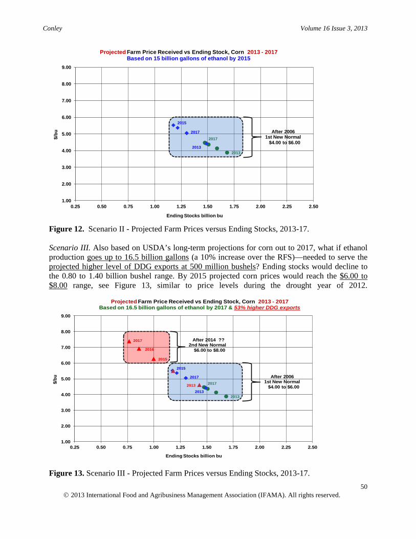
Figure 12. Scenario II - Projected Farm Prices versus Ending Stocks, 2013-17.

Scenario III. Also based on USDA’s long-term projections for corn out to 2017, what if ethanol production goes up to 16.5 billion gallons (a 10% increase over the RFS)—needed to serve the projected higher level of DDG exports at 500 million bushels? Ending stocks would decline to the 0.80 to 1.40 billion bushel range. By 2015 projected corn prices would reach the $6.00 to $8.00 range, see Figure 13, similar to price levels during the drought year of 2012.

Figure 13. Scenario III - Projected Farm Prices versus Ending Stocks, 2013-17.



51

Conclusions for the Scenarios It is probable that events –such as the current U.S. monetary policy of expanding the money supply, a Renewable Fuel Standard mandating 15 billion gallons of ethanol in the fuel supply, and the growing export market for distillers' grains—while individually may not have much impact, but taken collectively could result in a tipping point for the future production of ethanol and distillers' grain that would be a major increase from recent norms. The corresponding derived demand for corn, relative to the projected supply, would significantly affect the price levels for corn. From an industry analyst's perspective, it should be noted that the scenarios do not need to be viewed as static situations. Like using radar to track an emerging weather event, in the case of the third scenario it is possible to monitor on a monthly basis the exports of DDGs to leading countries like China, Mexico and Canada, along with total exports, to see if a higher export scenario begins developing. Since the scenario is looking forward five years, if exports do increase over time, then the relative probability of the third scenario being realized increases. If exports remain at current levels over the next two, three or four years, then the probability of realizing the scenario diminishes. Concurrent tracking of the money supply, the trade-weighted index for corn, and the RFS mandate provides additional insights into the probability of a third scenario being realized. The practice of tracking makes the analysis dynamic in contributing to a strategic plan. Implications for Management and Academia Imagine being in the role of an industry analyst or economist employed by a large multi-billion dollar company, or as a consultant to the same. In that role the person would be responsible for presenting an external environmental analysis to senior managers and board members who have substantial knowledge about various aspects of the industry. In addition, when presenting probable scenarios the person would be responsible for articulating the analysis in a way so recipients understand and have confidence in the results. Many of the senior managers and board members are likely to not be economists so a traditional analysis with a structured model may yield a "black box" effect and not be a credible, trusted approach. A regularly used method is the balance sheet approach, combined with graphical analysis and conditioned by an environmental scan, that explicitly shows expected cause and effect relationships. Managers and board members have a historical perspective on events and enough of an intuitive business sense that they understand and find such an approach as credible. The objective of this article was to illustrate, by example, the kind of analysis used for strategic planning by agribusiness firms and non-governmental organizations2. ____________________________________________________________________________ 2 The analysis in this article is based on actual experience. It was formally presented to an Ethanol Board of Directors for a major ethanol producing state in the U.S. and gave them a perspective they had not considered. As a result they have a strong interest in the ongoing research.



52

References Energy Information Administration. 2013. U.S. Oxygenate Plant Production of Fuel Ethanol

(Thousand Barrels). http://tonto.eia.gov/dnav/pet/hist/LeafHandler.ashx?n=PET&s=M _EPOOXE_YOP_NUS_1&f=A. [released date March 15, 2013]. Ethanol Producer Magazine, http://www.ethanolproducer.com/. 308 2nd Avenue North, Suite

304, Grand Forks, ND 58203, various issues in 2009-11. Food and Agricultural Policy Research Institute (FAPRI). 2010. FAPRI-MU US Biofuels, Corn

Processing, Distillers Grains, Fats, Switchgrass, and Corn Stover Model Documentation FAPRI-MU Report #09-10.

Gladwell, Malcolm. 2000. The Tipping Point: How Little Things Can Make a Big Difference.

Little, Brown and Company: New York. Luttrell, Clifton B. 1973. The Russian Wheat Deal - Hindsight vs. Foresight. Federal Reserve

Bank of St. Louis. http://research.stlouisfed.org/publications/review/73/10/Russian _Oct1973.pdf Morgan, Dan. 1979.Merchants of Grain. The Viking Press: New York, U.S. Department of Agriculture, Economic Research Service. 2012. Feed Outlook. FDS-10K.

Washington D.C., January 17, 2012. U.S. Department of Agriculture, Economic Research Service. World Agricultural Supply and

Demand Estimates (WASDE). Washington D.C., Various months, 1989-2012. U.S. Department of Agriculture. 2012. Office of the Chief Economist, World Agricultural

Outlook Board. Long-Term Projections Report OCE -2012-1. (Feb):66.

http://tonto.eia.gov/dnav/pet/hist/LeafHandler.ashx?n=PET&s=M_EPOOXE_YOP_NUS_1&f=A

http://www.ethanolproducer.com/

http://www.fapri.missouri.edu/outreach/publications/2010/FAPRI_MU_Report_09_10.pdf

http://www.fapri.missouri.edu/outreach/publications/2010/FAPRI_MU_Report_09_10.pdf



53

Appendix



54

Analysis for Strategic Planning Applied to Ethanol and ... · Applied to Ethanol and Distillers’...

Documents

Transcript of Analysis for Strategic Planning Applied to Ethanol and ... · Applied to Ethanol and Distillers’...