1

Department of Real Estate and Construction Management Thesis no. xxx

Name of Programme: Real Estate Management Master of Science, 30 credits

Real Estate Management and Financial Services

Analysis for Real Estate Investment of China

-Based on the Warning System of Monitoring Macro Economy Prosperity

Author Supervisor

Shu Jingying Mats Wilhelmsson

Song Jiawei Stockholm 2011

2

Title: Analysis for Real Estate Investment of China- Based on the Warning System of

Monitoring Macro Economy

Authors: Shu Jingying & Song Jiawei

Department: Department of Real Estate and Construction Management

Master Thesis number:

Supervisor: Mats Wilhelmsson

Keywords: real estate investment, leading indicator, granger causality, VAR models

Abstract

Real estate industry plays a significant role in high speed of economic development in

China. However, with increasingly high housing price and scare land resources, real

estate development is caught in a vicious circle. A large number of families could not

afford their housing while housing prices have no trend to decrease which leads to huger

gap between the rich and the poor and causes indirectly instability of society. Therefore,

creating a healthy and stable real estate investment market is extremely urgent. The

purpose of the thesis is to research the relationship between leading index of macro

economy prosperity and real estate investment based on the reality. We found that

leading indicator Granger causes real estate investment while real estate investment

Granger causes leading indicator at the same time. Based on that, this paper also

forecasts the real estate investment with VAR models in the following 7 years which

was proved to a circle of real estate market. In the light of our research, some target

suggestions are pointed out at last.

Master of Science thesis

3

Acknowledgement

We would like to express our sincere gratitude to our supervisor, professor Mats

Wilhelmsson, at The Royal Institute of Technology (KTH), for his feedback and

brilliant suggestions. His great patience and motivations support us to finish our hard

dissertation work. We also need to thank everyone at commissioner ’s office that gave us

valuable advice to improve our dissertation.

Last but not least, great thanks to our parents for their unconditional support and trust

when our stay in Sweden.

Stockholm May, 2011

Shu Jingying & Song Jiawei

4

Contents

1.Introduction ................................................................................................................................... 4

1.1 Background ......................................................................................................................... 4

1.2 Purpose ............................................................................................................................... 6

1.3 Outline ................................................................................................................................ 7

2.LiteratureReview ............................................................................................................................ 7

3. Methodology ............................................................................................................................... 10

3.1 Unit root ............................................................................................................................ 10

3.2 Co-integration and error correction .................................................................................. 13

3.3 VAR Model......................................................................................................................... 14

3.4 Granger causality .............................................................................................................. 16

3.5 Multiple-Step-Ahead Forecast .......................................................................................... 17

3.6 Impulse response function ................................................................................................ 18

4. Data ............................................................................................................................................. 19

5. Empirical Result ........................................................................................................................... 22

5.1 Result of Unit root tests .................................................................................................... 22

5.2 Result of Co-integration tests ............................................................................................ 24

5.3 Result of Error correction .................................................................................................. 25

5.4 Establishing VAR model ..................................................................................................... 25

5.5 Results of Impulse and Response Function ....................................................................... 28

5.6 Resulst of Granger causality test ....................................................................................... 30

5.7 Forecast of the Real Estate Investment in the Following 7 Years ...................................... 35

6. Summarys.................................................................................................................................... 38

7. Suggestions ................................................................................................................................. 40

8. Scope and Limitation of the study .............................................................................................. 41

Appendix ......................................................................................................................................... 43

References ....................................................................................................................................... 45

5

1. Introduction

1.1 Background

China’s rapid growth in the past years has been witnessed, even though the period of

global financial crisis. The total GDP increased from 364.5 billion RMB in 1978 to

3006.7 billion RMB in 2008, which was 82.5 times to 30 years ago. At the same time,

all industries expanded continuously. Although subprime crisis has moved forward

gradually to the end, expansion of domestic demand would still be the focal point of

future economic development in China, in which real estate played an important part.

Property investment (4044.18 billion) accounted for large share (23.4%) of total fixed

asset investment in 2008. (Yearly Book, 2009) As a pillar industry of national economy,

it promotes the boom of related industries, such as cement, steel and building materials.

In addition, this industry accelerates urbanization, improving the construction of urban

infrastructure. What’s more, the revenue and employment have been increased during

the course.

As a result of RMB appreciation, so much foreign hot money swarmed into China.

Owing to the irreplaceable role of high return, large amount of it pours in housing

market. In line with Qin. S and He. L (2010), this makes imbalance of real estate supply

and demand. Hot money belongs to venture capital, which focuses on luxury residential

buildings and villas, because of high margin. On the contrary, affordable housing or low

and medium residential are out of favor for developers. Due to the main source of fiscal

revenue and high added value, government encouraged its growth. Rapid rate led to

housing price beyond of people’s affordability. Overheating situation aroused people’s

thinking. China’s economy over-depended on real estate in the past years, which pushed

our economy into the abnormal situation. Instable factors come out, such as widening

the gap between the poverty and rich, distortion of the distribution of social wealth.

6

People expected for healthy and stable real estate market. These years, regulations

experienced the stages from inhibition of expansion for market demand, prevention

prices rising fast to encouragement of rational demand and change of investment-driven

economic growth.

In order to make a sustainable investment, many scholars took part in study actively

recently. Here, the real estate investment can be defined as the action that all kinds of

real estate companies develop the housing residencies, plants, warehouses, restaurants,

hotels, holiday villages, office buildings, as well as public facilities and land

development. (Yearly Book, 2009) Research fields referred to wide-ranging, such as

macroeconomic policy, the relationship between housing price or GDP and investment,

risk. However, there are seldom references regarding on how the warning system of

macro economy prosperity affected the investment, which consists of a series of

economic indicators to monitor the trend of macro economy and predict its development.

The warning system of macro economy prosperity will be used for this paper, including

leading, coincide and lagging indicator. Leading indicator refers to the data that change

before the overall increase or decrease of national economic cycle. The second one can

reflect the characteristics of fluctuation, and its turning point synchronizes with the

transformation of economy. The last one shows the effect after the rise and down. (Xie.

J. B, Wang. B. H, 2007)

1.2 Purpose

This paper will try to illustrate the relationship between macro economy prosperity and

real estate investment based on the reality. Within this context, the study of this issue is

of great significance. Investigation before real estate investment is in the initial stage in

China, especially based on the warning system of monitoring macro economy prosperity.

Through this analysis, policy makers could make effective adjustment on policies more

immediately and it would be beneficial for consumers to invest more rationally.

Additionally, the firms’ governors can master the overall situation and make a sensible

7

decision, which can promote the healthy development of real estate in China.

1.3 Outline

The reminder of the paper is divided into four parts. In section two, we will provide

literature review from home and abroad references. One area—warning system of

macro economy prosperity, which should have an effect on property investment, has

been neglected by most of the people. Methodologies will be presented in section three,

including the introduction of unit root, co-integration and error correction, VAR model,

Granger causality, impulse response function. The description for data will be illustrated

in Section four. Section five will focus on analysis and results according to the previous

study. Section six presents the summary. Suggestions will be given in the section seven.

In the last section, the scope and limitation of the this research will be discussed.

8

2. Literature Review

Looking at the world, real estate investment has increasingly affected the overall

economy. The development of global real estate investment benefits from the

liberalization and internationalization of financial market. The evaluation of market

fundamentals and institutions of recipient localities are the key factors to consider.

(Zhu.J.M, Sim.L.L, Zhang.X.Q, 2006) For the global investment, cost of international

real estate diversification should also be taken into account. The cost can be reduced by

invest in public property companies, who pays much attention to their local and

domestic market. (Eichholtz.P, Koedijk. K, Schweitzer.M, 2001)

For different countries, the study key points of housing investment are like chalk and

cheese. For example, in UK, The monetary policy has larger impact on residential

investment than fiscal policy. However, the power of money has disappeared in 1980s

of post deregulation. So the causality between residential investment and

macroeconomic variables had been changed during that time. (Hasan.M.S, Taghavi.M,

2002) In France, Arrondel.L (2001) compares the differences between housing

investment and consumption, which can influence the purchase decision as an

occupier-owner or landlord. However, the researches of real estate investment in

Australia are focused on cost and return of small investment companies and individual

investors, who account for majority of real estate investment market. (Eves, C. & Wills,

P., 2003)

In China, real estate investment is a totally different activity, upstream concerning for

government monopoly, while downstream related to common people. There is a game

between selling land at a high price and creating harmonious society for the government.

For the common people, stable and affordable housing market can increase the

happiness index. So the macroeconomic control for the real estate investment becomes

so important. Chen.B.G (2010) said the macroeconomic control in China went through

9

five years. The central government regulated the real estate market due to the high

growth of housing price in 2005~2006. The measures were mainly contraction fiscal

and monetary policy, including tightening of the mortgage, increasing the percentage of

down payment. Then the housing price calm down, and the property market recessed.

Nevertheless, due to the adjustment in 2007, the market boomed. One year later,

contraction policy was again brought it to the downturn. It was not until to 2009,

Chinese government realized that the role of real estate as pillar industry, which would

have an effect on expansion of domestic demand and economic growth in the prosperity

of global financial crisis. On the contrary, too far away from balance, abnormal speed of

development turned up.

No matter how many stages of real estate investment experienced, it is closely related to

macro economy at the time. Many scholars paid much attention to research the

relationship of these two aspects. Zhang.X.J and Sun.T (2006) analyzed the real estate

cycle and financial stabilization, including the growth, policy and macro aspect, by

using quarterly data of 1992~2004. Either the real estate industry or the housing price

would go up. It was reflected on credit risk and government guarantee risk that how the

real estate cycle affects stable finance. Wu.S (2010) studied the interaction between the

real estate investment and economic growth of the past 15 years, which showed that the

two variables had long term dynamic equilibrium. The increase of production factors

supply and productivities led to economic growth, consisting of the improvement of

industrial structure, scale economy, technology innovation, capital and labor. All of

these played a significant role in real estate investment and development. Sheng.C.M &

Fang.Z.D (1999) pointed that the change of national economy in China will lead to the

change of real estate investment. According to Duan.Y.Y and Tian.H (2009), real estate

investment and housing price were positively correlated by analysis of real estate

investment and GDP growth, housing price and people’s disposable income. Both of the

growth rate of property investment and housing price were much faster than national

economy. In the long run, the industry of real estate should keep pace with national

economy, people’s disposable income. When national economy growth rate increased

10

1%, the real estate investment went up 12.7%, vice versa. The larger the investment

range fluctuates, the slower the development for this industry. So the target of

macroeconomic control was to reduce the swing, making the growth sustainable.

(Wang.M, Tang.X.F, 2000)

Searching the previous study of real estate investment in China, most people focused on

economic growth or housing price. Although they were some of the most significant

factors, warning system of monitoring macro economy prosperity has been neglected,

which may affect the confidence of investors and their behaviors. In the following of the

paper, we will discuss the relationship between these two aspects.

11

3 Methodology

When choosing methodology to analyze, several methodologies occur to us. They are

theoretical analysis, fundamental analysis and VAR models analysis. However,

theoretical analysis is too abstract for such a practical problem and could not reflect

direct information for government or investors to take measures accordingly.

Considering fundamental analysis, since fundamentals in real estate investment are hard

to measure and quantified and we have no access of data of fundamentals in real estate

investment, it’s also not the main focus of this study. Meanwhile, in recent researches,

VAR models have been proven to be one of the most effective and easiest methods in

studying the relationship of variables in the housing market as well as forecasting

variables. For example, Zhou, Z. (1997) examined demand in the existing single-family

housing market and concentrated on relationship between sales volume and median

sales price and furthermore forecasting sales and prices of single-family housing in the

United States using VAR models. However, the limitation of VAR models is that they

require a large number of data in models. Therefore, we collect a long-term period

monthly data of 20 years for variables respectively.

In this part, the methodology employed in the thesis will be introduced. Unit root test is

to examine whether the time series data are stationary, which is essential for establishing

VAR models since non-stationary data are not supposed to be used in regression models

to avoid spurious regression. There are three kinds of unit root tests test for different

properties of data and we could choose one according to the plot of time series. If they

are non-stationary, difference the data to make them stationary and then we perform

co-integration test to examine whether they share similar stochastic trends. If they are

not co-integrated, any regression relationship between time series is fake. VAR models

are used to describe the interrelationship between two stationary variables, which is also

an effective tool to forecast economic variables. (Hill R. C, Griffiths, E. W & Lim, C. G,

2008)

12

3.1 Unit root

In the autoregressive model,

yt = c + βyt−1 + εt (1)

Where c is a constant, β is coefficient, εt is the sequence of error items of zero mean,

and t=1, 2, 3 … T. If the absolute value of β equals to one, leading to non-stationary

time series, the process of (1) is called random walk, which means that y at time t

depends on the previous value of yt−1. Random walk is a special example of unit root

process, in which the coefficient of yt−1is one at the first order of autoregressive model.

According to Wooldrigde (2005), unit root test has become increasingly important in the

modern time series econometrics. If the unit root exists, the normal approximations are

no longer valid even in the large sample sizes. Although there is many a method for this

kind of test, here Dickey-Fuller test will be chosen, since it is the most popular and

easiest one.

Subtracting yt−1 from both sides of equation (1), and defining θ=β − 1, the

Dickey-Fuller could be:

∆yt = c + θyt−1 + εt (2)

Where ∆yt is the first order difference of sequence yt . Wooldrigde (2005) points that

if we assume the null hypothesis of H0: θ = 0, the alternatives H1: θ < 1. Given that

there is a unit root for (2), then ∆yt = c + εt , mean linear exists in the change of yt。

So the appropriate hypothesis should be H0: θ = 0. For this test, t statistic will be used,

which is defined as:

t =θ−0

se (θ) (3)

Where se(θ) is the standard error of θ. The Dickey-Fuller test will be performed for

real estate investment and leading indicator. And the result will be presented in the next

section.

13

3.2 Co-integration and error correction

Once the Dickey-Fuller test done, if the two series of yt and xt experience unit root

process, it can be said to be integrated at order one or I (1). Generally speaking, the

linear combination of them is still I (1). Nevertheless, it could be the weakly dependent

process or I (0). If it is in this case, the two series are co-integrated at order one, which

implies they have constant mean, constant variance.

In order to check the co-integration, we define a new formula first,

yt = α + βxt + ut (4)

Then we have to check if the residuals of ut = yt − α − βxt is stationary. If we refuse

the null hypothesis of unit root in｛ut｝, yt and xt are co-integrated. Otherwise, the two

sequences are not co-integrated. The spread between them could be very large, and no

tendency for them to come back together. If we go as it is, we will run a spurious

regression, making no sense for the long-run relationship.

There are a number of methods can be used for testing co-integration. For instance, we

can use Dickey-Fuller (DF) or Augmented Dickey-Fuller (ADF). Gujarat (2004)

elaborates that ut is based on regressed coefficient β, so the DF or ADF critical

significant value may not suitable. Under these circumstances, Engel-Granger (EG) or

Augmented Engel-Granger (AEG) test can be the better choice. When we performed a

unit root test on the residual from Equation (4), we will get the below relationship:

∆ut = γut−1 + c. (5)

In this study, we will test co-integration between real estate investment and leading

indicator. If yt and xt are not co-integrated, we might consider a dynamic model in

first differences, i.e:

∆yt = c + αt + θ∆yt−1 + γ0∆xt + γ1∆xt−1 + ut (6)

Where ut has zero mean. From the above, we can find long-run propensity as well as

lags distribution. If yt and xt are co-integrated, the error correction term should be

added to (5), such as δ(yt−1 − βxt−1), and the model could be error correction model.

14

For simplicity, the model can be written as: (Wooldridge, 2005)

∆yt = c + γ0∆xt + δ(yt−1 − βxt−1) + ut (7)

According to Gujarati (2004), ∆yt depends not only on ∆xt but also on yt−1 −

βxt−1

3.3 VAR Model

Wooldridge (2005) points out that if the series of y and x follow

yt = δ1 + α1yt−1 + γ1xt−1+α2yt−2 + γ2xt−2 + ⋯ (8)

and

xt = δ2 + α1yt−1 + γ1xt−1+α2yt−2 + γ2xt−2 + ⋯ (9)

which is the vector autoregressive (VAR) model. Each equation has a zero expected

error.

There are types of criteria. Here, we discuss between in-sample and out-of-sample. In

regression, in-sample is better, using R-square.

R2 =SSE

SST= 1 −

SSR

SST (10)

SST means the total sum of squares, SSE equals to explained sum of squares, and SSR

denotes to the sum of squared residuals.

As a penalty for imposing independent variable to increaseR2, adjusted R-squared has

been developed.

R 2=1-SSR /(n−k−1)

SST /(n−1) (11)

Here k means the number of independent variables.

It may be better for us to choose the second criteria, since forecasting is not an

in-sample issue. If there are e+f observed values, the first e values can be used in the

regression model, while the later f ones can be applied for forecasting. Besides those,

15

we also have to consider Akaike information criterion (AIC), Schwarz Information

criterion (SIC), forecast χ2 (chi-square), Final prediction error (FPE) and Hannan-Quinn

Information Criterion (HQIC).

Gujarati (2004) elaborates another penalty for adding independent variables is to use

Akaike information criterion (AIC), in which the definition is:

AIC = e2k/n δ i2

n= e2k/n SSR

n (12)

Conveniently, the above can be written as:

lnAIC = (2k

n) + ln(

SSR

n) (13)

Where lnAIC is the log of AIC and 2k/n means the penalty factor. The lower AIC the

model has when comparing, the better it is. What’s more, this criterion fits not only the

in-sample but also the out-of-sample. Similar to AIC, SIC can be defined as:

SICnk/n u 2

n= nk/n SSR

n (14)

Or

lnSIC =k

nlnn + ln(

SSR

n) (15)

Here k

nlnn is the penalty factor. Likewise, the model with the lowest SIC is preferred.

Given n observations in the regression sample, we want to use them to forecast the

model for the added t observations. So the forecast chi-square (x2 ) can solve the

problem, which can be defined as:

χ2 = u i

2n +tn +1

δ 2 (16)

Where u i is the forecast error for time i (i=n+1, n+2 … n+t) based on the fitted model

and the post sample period, and δ is the error from ordinary least square of the fitted

regression.

Final prediction error (FPE) is another information criterion. According to Akaike

(1970),

16

FPE = n+p

n−p

SSR m

n (17)

Where n is the sample size, m is the lags, p=m+1 if series of yt and xt are not

co-integrated, while p=m+2 if they are.

In 1979, Hannan and Quinn found alternative information criterion to AIC and SIC,

which can be written as:

HQIC = nln SSR

n + 2kln(lnn) (18)

Here k is the number of parameters.

3.4 Granger causality

According to Granger (1969), the causality is defined as if it is better to forecast yt

based on all obtainable data than if the data is apart from xt , we say xt is causing yt .

Wooldridge (2005) tells us that z Granger causes y when E (yt｜𝐼𝑡−1) ≠ E(yt｜𝐽𝑡−1),

where the information of past y and x is included in 𝐼𝑡−1, while only information of y is

included in 𝐽𝑡−1. Provided the linear model and the lags of y have been chosen, it is easy

to test the null hypothesis in which x does not Granger y. At first, the autoregressive

model of y has to be estimated, as well as t and F tests are used to determine how many

lags of y. The lags of quarterly and monthly data are more than that of yearly data. We

can take a simple example, given E (ut｜𝑦𝑡−1 ,𝑦𝑡−2 ,𝑦𝑡−3 ,… = 0)

yt = δ0 + α1yt−1 + α2yt−2 + α3yt−3 + 𝑢𝑡 (19)

As long as the autoregressive model of y has been decided, the lags of x can be

determined, which is less significant since x does not Granger y. If one lags of x is

added to the above formula, t test can be used to examine the significance. While if two

or more lags of x are added, F test can be used for the joint significance, such as

yt = δ0 + α1yt−1 + α2yt−2 + α3yt−3 + γ1xt−1 + γ2xt−2 + 𝑢𝑡 (20)

17

3.5 Multiple-Step-Ahead Forecast

Given that we want to forecast yt+1 at time t and s (s<t), the VAR［yt+1 − E(yt+1｜𝐼t)］

≤ VAR［yt+1 − E(yt+1｜𝐼s)］, which is to say the more information the less error

variances. Assuming｛yt｝abides by autoregressive progress of order one, or ［AR(1)］,

such as

yt = c + βyt−1 + ut

E(ut｜𝐼t−1)=0, 𝐼t−1 = {yt−1 , yt−2 , yt−3,… },

where the variance σ2of {ut} is constant. As a result, the one-step-ahead forecast has

the variance of σ2. In the multiple-step-ahead forecast, through repeated substitution,

we get

yt+h = 1 + β + ⋯+ βh−1 c + βh yt−1 + βh−1ut+1 + βh−2ut+2 + ⋯+ ut+h (21)

We expect all the ut+j to be zero, for j≥1, at time t. Therefore,

E(yt+h｜𝐼t) = 1 + β + ⋯+ βh−1 c + βh yt−1 (22)

Where the forecast error is et,h = βh−1ut+1 + βh−2ut+2 + ⋯+ ut+h . So the Var

(et,h ) = σ2 1 + β2 + ⋯+ β2 h−1 . When β2 < 1, Var (et,h ) = σ2/(1 − β2). If

β2 = 1, ft,h=ch+ yt , and Var (et,h ) = σ2h.

Likewise, it is also applied to VAR model. Supposing

yt = δ0 + α1yt−1 + γ1xt−1 + ut (23)

and

xt = θ0 + α1yt−1 + γ1xt−1 + vt (24)

If we wish to forecast yt+h at time t, we can get

E(yt+h｜𝐼t) = δ0 + α1E(yt+h−1｜𝐼t) + γ1E(zt+h−1｜𝐼t). (25)

As a result of E ut+h 𝐼t = 0, the above can be written generally down as:

f t,h = δ 0 + α 1f t,h−1 + γ 1g t,h−1 (26)

18

So as to know how precise we forecast y for this out-of-sample, the root mean squared

error (RMSE) and the mean absolute error (MAE) can be used, including:

RMSE=(m−1 e n+h+12m−1

h=0 )1/2 (27)

and

MAE=m−1 ｜e n+h+1｜m−1h=0 (28)

Here e n+h+1 = yt+h+1 − f t+h. We prefer the smallest RMSE and MAE in order to

minimizing the largest absolute values of the forecast errors. (Wooldridge, 2005)

3.6 Impulse response function

Gujarati (2004) sets forth that the coefficients of VAR model are difficult to interpret, so

we introduce impulse response function (IRF). The IRF illustrates how a shock of one

standard deviation of error term (δ1 or δ2) influences endogenous variables. Take

Equation (7) and (8) for example. Suppose δ1 increase through a shock of one standard

deviation in y regression. Such a change will influence y at present as well as in the

future. Since y appears in x regression, the shock of δ1 will have an effect on x.

Analogously, such a shock in δ2 of x regression will lead y to change.

19

4 Data

The leading index will be chosen to represent the warning system of monitoring macro

economy prosperity in according to Table 1, since the property construction depends on

steel production, iron ore production, steel stocks, cement stock, infrastructure loan,

number of projects started, also people’s affordability reflects on wages of individuals,

all of which are comprised in leading index. Moreover, econometric method to forecast

real estate investment is seldom used in China. The data used in this thesis are leading

index of macro economy prosperity and real estate investment index which are monthly

data from January 1990 to September 2010 obtained from National Bureau of Statistics

of China.

Leading index of macro economy prosperity, denoted as ldind, changes in advance

compared to fluctuation of macro economy cycles. For instance, if some indicators

achieve peaks or troughs earlier than macro economy cycles for several months, they

are called leading indicator, which could predict the economic situation to some extent

in following years. (Xie Jiabin & Wang Binhui, 2007)

20

21

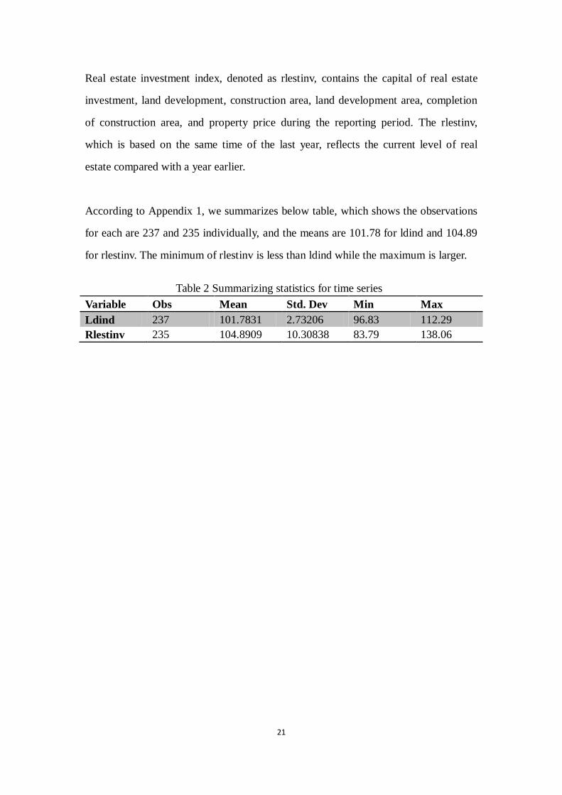
Real estate investment index, denoted as rlestinv, contains the capital of real estate

investment, land development, construction area, land development area, completion

of construction area, and property price during the reporting period. The rlestinv,

which is based on the same time of the last year, reflects the current level of real

estate compared with a year earlier.

According to Appendix 1, we summarizes below table, which shows the observations

for each are 237 and 235 individually, and the means are 101.78 for ldind and 104.89

for rlestinv. The minimum of rlestinv is less than ldind while the maximum is larger.

Table 2 Summarizing statistics for time series

Variable Obs Mean Std. Dev Min Max

Ldind 237 101.7831 2.73206 96.83 112.29

Rlestinv 235 104.8909 10.30838 83.79 138.06

22

5 Empirical Result

5.1 Result of Unit root tests

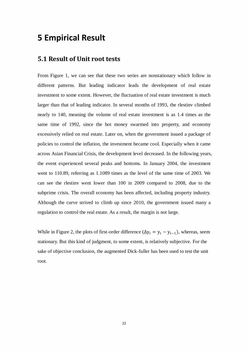
From Figure 1, we can see that these two series are nonstationary which follow in

different patterns. But leading indicator leads the development of real estate

investment to some extent. However, the fluctuation of real estate investment is much

larger than that of leading indicator. In several months of 1993, the rlestinv climbed

nearly to 140, meaning the volume of real estate investment is as 1.4 times as the

same time of 1992, since the hot money swarmed into property, and economy

excessively relied on real estate. Later on, when the government issued a package of

policies to control the inflation, the investment became cool. Especially when it came

across Asian Financial Crisis, the development level decreased. In the following years,

the event experienced several peaks and bottoms. In January 2004, the investment

went to 110.89, referring as 1.1089 times as the level of the same time of 2003. We

can see the rlestinv went lower than 100 in 2009 compared to 2008, due to the

subprime crisis. The overall economy has been affected, including property industry.

Although the curve strived to climb up since 2010, the government issued many a

regulation to control the real estate. As a result, the margin is not large.

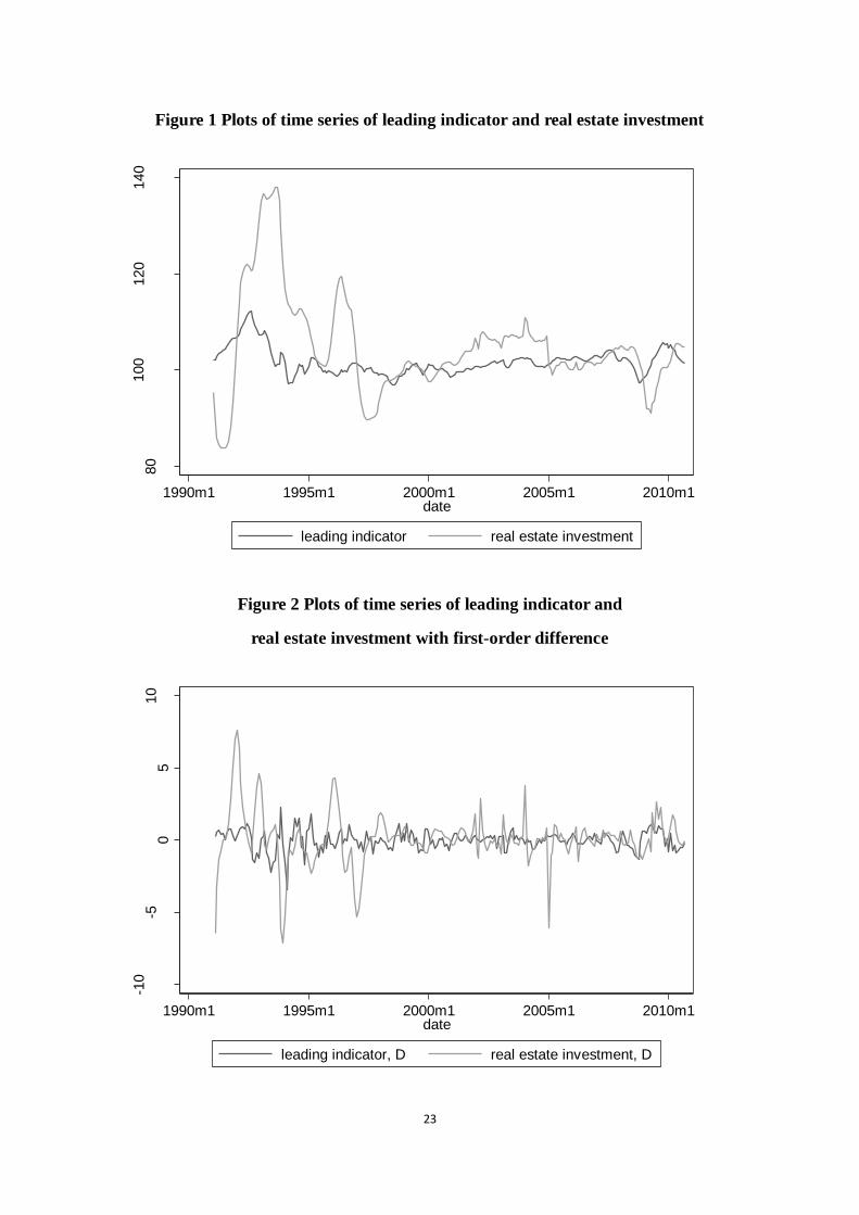
While in Figure 2, the plots of first-order difference (∆yt = yt − yt−1), whereas, seem

stationary. But this kind of judgment, to some extent, is relatively subjective. For the

sake of objective conclusion, the augmented Dick-fuller has been used to test the unit

root.

23

Figure 1 Plots of time series of leading indicator and real estate investment

Figure 2 Plots of time series of leading indicator and

real estate investment with first-order difference

80

100

120

140

1990m1 1995m1 2000m1 2005m1 2010m1date

leading indicator real estate investment

-10

-50

510

1990m1 1995m1 2000m1 2005m1 2010m1date

leading indicator, D real estate investment, D

24

Using Stata 10.0, we do the unit root test for ldind and rlestinv, including constant but

no time trend. Since they are monthly data, 12 lags have been chosen. According to

Table 3, test statistics for these two are -2.429 and -2.045 respectively, both of which

are larger than the critical value. As a result, we cannot reject the null hypothesis that

they are nonstationary. So we assume they are at I(1).

Table 3 Augmented Dickey-Fuller test for unit root

5.2 Result of Co-integration tests

Earlier, we found there exit unit root in the above two series. Now, we have to know if

they are co-integrated in order to avoid spurious regression. Let us first estimate

rlestinv on ldind and obtain following regression:

rlestinv = 1.256961ldind − 23.04795

Since rlestinv and ldind are respectively nonstationary, it is possible that this

regression is spurious. But when we performed a unit root test on its residuals, we

conclude the following results:

∆ut = −0.0624216ut−12 + 0.0992208

t = −5.19 (0.83)

R2 = 0.1095

The p-value for ut−1 is 0.000, which is to say the two series are I(0). In other words,

the regression residuals are stationary, so that leading indicator and real estate

investment are co-integrated in the long run, implying they are moving together in the

long run. Thus, 1.256961 represents the long-run marginal propensity to real estate

investment.

25

5.3 Result of Error correction

We just showed that rlestinv and ldind are co-integrated. However, there may be

disequilibrium in the short period. Therefore, we have to add the error term to identify

the short term behavior.

D. rlestinv = 0.0423247D. ldind − 0.0656059L12. ehat + 0 .0674634

t = 0.27 −6.14 ( 0.64)

R2 = 0.1482

Accordingly, the error term is zero, meaning that rlestinv adjusts to changes in ldind

in the same time period. Short-run shift in ldind have a positive impact on short-term

changes in rlestinv. We can interpret 0.0423247 as the short-run marginal propensity

to real estate investment.

5.4 Establishing VAR model

Based on the variables of leading indicators and real estate investment, the vector

autoregressive model has been established. In order to determine the lags, the

information criterion will used to choose (see Table 4).

Table 4 The information criterion for VAR lags

In the practical application, the lag period is the problem we have to think about. The

larger the lags, the more it can reflect the dynamic characteristics. On the contrary, the

larger the lags, the more unknown variables, and the less the degree of freedom. So

there is a trade-off between lags and degree of freedom. As the above shown, lag 4 is

26

the best choice according to the five criterion. Then VAR (2) would be set up. The

formula is ( see Table 5)

rlestinvldind

= −6.7833.776

+ 1.724 −0.220 0.027 1.401

rlestinvL 1ldindL 1

+ −0.685 0.285 −0.0008 −0.184

rlestinvL 2ldindL 2

+

0.095 −0.220 −0.012 −0.669

rlestinvL 3ldindL 3

+ 0.123 −0.054 −0.022 0.423

rlestinvL 4ldindL 4

+ ε1ε2

27

Table 5 VAR model

rlestinv means real estate investment index, ldind means leading indicator. L1, L2,

L3, L4 mean the first, second, third and forth lag from period t respectively.

28

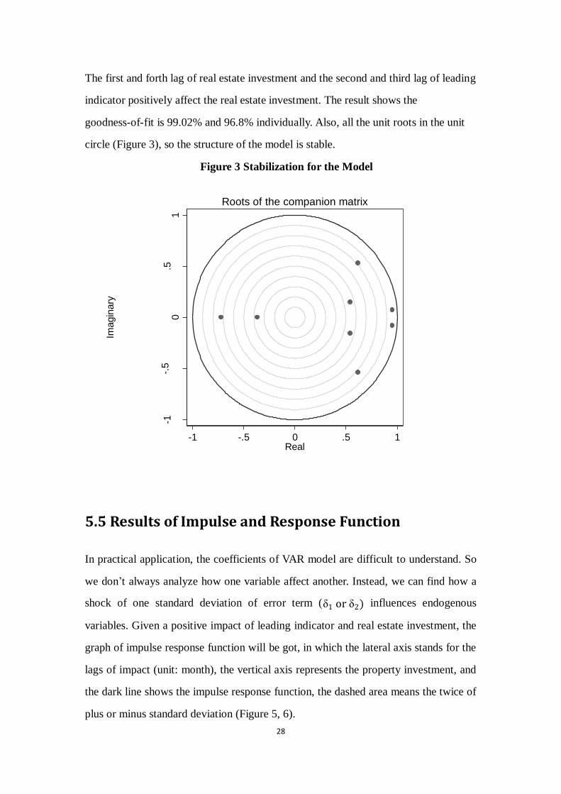
The first and forth lag of real estate investment and the second and third lag of leading

indicator positively affect the real estate investment. The result shows the

goodness-of-fit is 99.02% and 96.8% individually. Also, all the unit roots in the unit

circle (Figure 3), so the structure of the model is stable.

Figure 3 Stabilization for the Model

5.5 Results of Impulse and Response Function

In practical application, the coefficients of VAR model are difficult to understand. So

we don’t always analyze how one variable affect another. Instead, we can find how a

shock of one standard deviation of error term (δ1 or δ2) influences endogenous

variables. Given a positive impact of leading indicator and real estate investment, the

graph of impulse response function will be got, in which the lateral axis stands for the

lags of impact (unit: month), the vertical axis represents the property investment, and

the dark line shows the impulse response function, the dashed area means the twice of

plus or minus standard deviation (Figure 5, 6).

-1-.

50

.51

Imagin

ary

-1 -.5 0 .5 1Real

Roots of the companion matrix

29

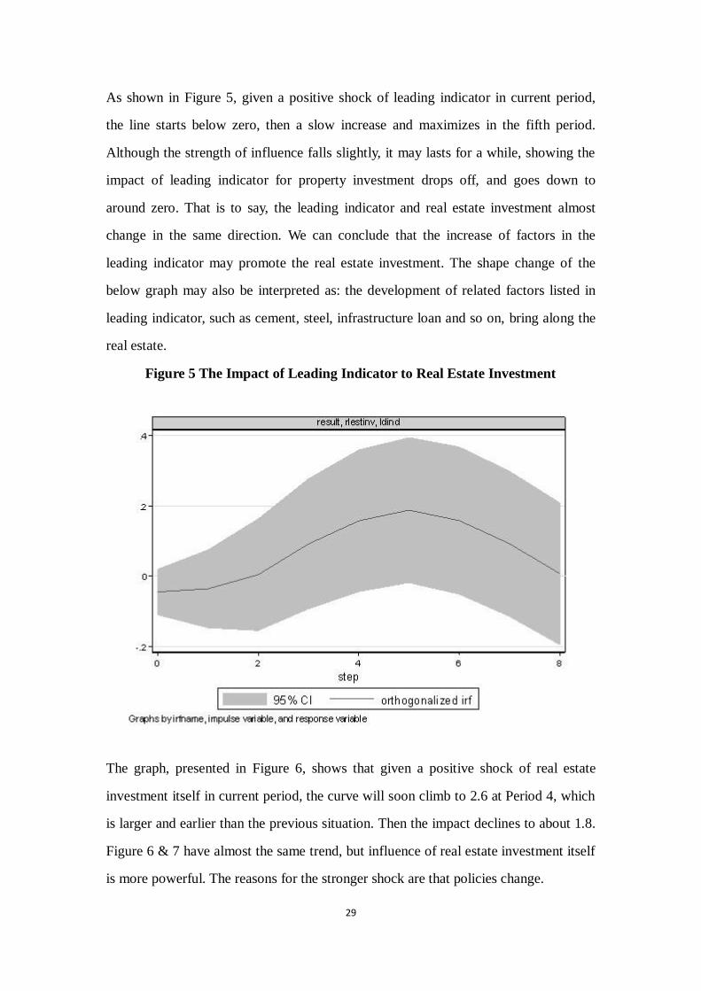
As shown in Figure 5, given a positive shock of leading indicator in current period,

the line starts below zero, then a slow increase and maximizes in the fifth period.

Although the strength of influence falls slightly, it may lasts for a while, showing the

impact of leading indicator for property investment drops off, and goes down to

around zero. That is to say, the leading indicator and real estate investment almost

change in the same direction. We can conclude that the increase of factors in the

leading indicator may promote the real estate investment. The shape change of the

below graph may also be interpreted as: the development of related factors listed in

leading indicator, such as cement, steel, infrastructure loan and so on, bring along the

real estate.

Figure 5 The Impact of Leading Indicator to Real Estate Investment

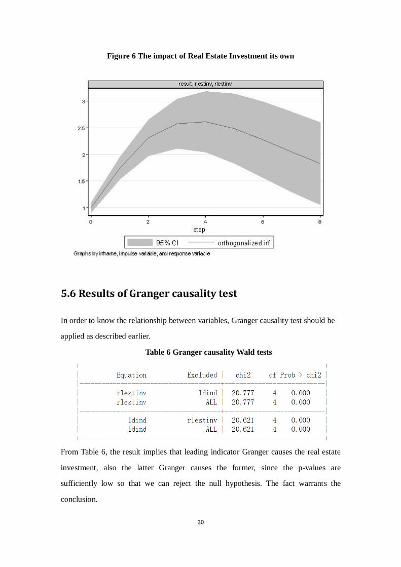
The graph, presented in Figure 6, shows that given a positive shock of real estate

investment itself in current period, the curve will soon climb to 2.6 at Period 4, which

is larger and earlier than the previous situation. Then the impact declines to about 1.8.

Figure 6 & 7 have almost the same trend, but influence of real estate investment itself

is more powerful. The reasons for the stronger shock are that policies change.

30

Figure 6 The impact of Real Estate Investment its own

5.6 Results of Granger causality test

In order to know the relationship between variables, Granger causality test should be

applied as described earlier.

Table 6 Granger causality Wald tests

From Table 6, the result implies that leading indicator Granger causes the real estate

investment, also the latter Granger causes the former, since the p-values are

sufficiently low so that we can reject the null hypothesis. The fact warrants the

conclusion.

31

5.6.1 In the Period of 1990~1996

Since early 1990’s, China’s experienced fast development of economic transition. By

establishing the goal of socialist market economy in 1992, the expansion came to the

climax. The government wanted to devote major effort to develop post and

telecommunications, chemical industry, infrastructure, energy resources in advance,

which stimulated the means of production, such as steel and cement. The situation

excessively relying on the investment came into being. The real estate craze acted

according to the circumstances, especially in Hainan province. The price was about

RMB 1000 per square meter at first, while went up to RMB 3000, even 10,000 yuan

between the year 1991 and 1993. (Niu. R. B and He. B, 2002)

In order to eliminate the side effect of overheating economy, contracted monetary

policy was adopted. At the same time, the State Council issued ―The Suggestions on

Present Economic Situation and Strengthening the Macro-control‖. The effect first

reflected on the production of raw material, infrastructure loan, which reflected on the

declining trend of leading indicator. As a result of the warning signal for future

economy, entrepreneurs’ confidences are greatly dampened, further affecting their

decision. Due to the hysteretic nature, the decrease in property investment exhibited

later. With the decreasing of leading indicator in the middle of 1990’s, the overall

trend of fix asset investment declined, although there was a little fluctuation.

Generally speaking, the developers made investment decisions in the booming cue.

When the warning system illustrated depression, capital flows to other fields. Unlike

other industries, real estate itself referred to lags. Sometimes, the leading indicator

had gone down during the process of construction while it was too late to adjust for

developers. Once the projects completed, the entire environment changed. Since the

high price wasn’t in people’s affordability, the demand for the housing went down.

Real estate companies had difficulty in taking a step of financing as a result of the

policy. Seldom new projects are started, but more space available on the market.

32

Some projects cannot be completed. A lot of property firms went to bankrupt due to

lack of loans when the old ones expired.

In addition, real estate itself is a dog-eat-dog industry so that some state-owned firms

could not adapt to the fast changing market for the sake of the rigid system. On the

other hand, overheated property investment is the engine for economy. The peak of

real estate attracted the authorities’ attention. They were aware that if the growth

relied mainly on real estate, how would the vacant properties go and how would the

inflation turn down. Soft-landed economic policy came out accordingly. The fiscal

expenditure decreased, while the interest rate went into the other direction. Through

these measures, currency circulation reduced. (Liu. W, 2005) As a result of depression,

output of raw material, primary energy and light industries would decrease. So did the

infrastructure loans and started projects. That is to say, real estate investment turned

down the economy, reflected on leading indicator.

5.6.2 In the Period of 1997~2004

Unfortunately, Asian financial crises broke out in 1997, which influenced China’s

foreign trade deeply, only with the degree of contribution of 0.2 in economic growth.

Decreasing export led to less foreign investment, as well as higher unemployment.

Finally, national economy was inevitably affected. (Cao. J. F, L. L, 2008) Most kinds

of industries, listed in the leading indicators, showed a tendency of decrease, which

influenced real estate investment.

In order to pull through, the Chinese government took the measures of slack fiscal and

monetary policy to expand the domestic demand. On one hand, the proactive fiscal

policy opened up a market for the weak domestic demand, such as the long-term

construction bond. From 1998 to 2002, we had issued this kind of bond for 660 billion

RMB. A package of polices were adopted like increasing tax refunds to exporters,

33

cutting regulation tax on fixed asset investment orientation by half at first then the all

between 1998 and 2000. On the other hand, the prudent monetary policy was benefit

to stabilize the prices. The reserve ratio was lowered from 13% to 8% in 1998, while

the interest rate was reduced in four successively running. (Yuan. Z. X, 2010) This

regulation stimulated the steel price slightly increase of RMB 500 to RMB 2630 per

ton. Higher price made the suppliers interest in this industries. So did the other

products not just related construction materials as a result of the low reserve ratio and

interest rate. ―The Management for Personal Housing Loan‖ was published by

People’s Bank of China in 1998, allowing for all commercial bank to offer loans to

individuals who wanted to buy a house. It seemed surprising but made sense.

In spite of a bit fall, the leading indicator and real estate investment kept the overall

upward trend until 2004. The iron, steel and cement were produced 110, 109 and 335

billion ton respectively in January 2001. Later, all of these went to 188, 218 and 755

billion ton individually at the same time of 2004. (Yearly Book, 2009) Meanwhile, the

export, energy and metals boomed which promoted the leading indicator. The index,

because, implied good future economy, the property firms found business

opportunities.

The real estate investment got golden age. Different from the previous cycle, it

progressed smoothly. The government and developers tended to pursue the rational

mode. Consequently, this round, which showed the expansion period, advanced wave

upon wave. (Zhou. X. Y, 2009)

5.6.3 Ever Since 2005

The latest phase lasted from 2005. With the dramatic increase of national economy, all

professions and trades appeared a scene of prosperity. The production related

construction material continued to rise. By perfecting the laws and regulations of

34

foreign trade, exports further contributed to the economy. In the mean time, M1 was

on the rise. The high growth needed large number of workers, thus rural population

swarmed into the cities, enlarging the urbanization. (Chen. R. L, 2009) A new round

of real estate investment boom began.

In this period, the lag effect performed most significantly. The leading indicator

preceded property investment a few months, both of which got another peaks in 2007.

Yet unpredictable American sub-prime crises shocked us a lot. Foreign export

decreased sharply, occurring economic weakness. For example, steel 482 billion ton,

cement 1208 billion ton in August 2007, while both had 3 billion ton decrease over

the same period of 2008. (Yearly Book, 2009) The investment went to the bottom in

the early 2009. According to Yuan. Z. X (2010), this time is different from the last one.

This time created double burden. For the outside, decreasing foreign customers

affected our export market. For the inside, inflation, over capacity, unbalanced

structure made the economy downturn objectively. By effective and efficient fiscal

and monetary policy, the factors of leading indicator gradually got warm again,

showing the prosperity for future environment. The decision-makers were greatly

encouraged, then property investment was back on stage.

However, in the recent one year, irrational demand and development led to the

housing price seriously exceed people’s affordability. In order to control the

investment overheating, central government published a package of laws and

regulations, such as increasing the down payment of the second apartment and interest

rate, imposing property tax and so on. Psychological warfare among developers,

consumers, government and banks quietly began. Since possessing cost increased, the

buyers and the renters were in a wait state for a long time. They couldn’t decide to

buy or not to buy, hoping the price to decrease to a psychological level. But for

developers, the situation was another matter. The confidence and construction were

influenced seriously in deed. Obtaining land and financing have been affected

significantly. On the contrary, some new properties were set abnormally high price to

35

stop sale. Once the action lasted for a while, the capital chain might face tremendous

pressure. The developers trapped in the dilemma of decreasing the price or not,

investing or not. In regard to regional governments, the revenue would decrease since

it relied on land transfer fee. What’s more, all of city and town land use tax, housing

property tax, farm land occupation tax turned over to local governments. The above

might account for 50%-70% fiscal revenue. (Lin. Y. Q, 2010) By implementing the

new policy, this part would be impaired a lot. As a result, the construction processes

for affordable housing would be affected. Control or not puzzled the officials. Another

aspect could not be ignored——banks. Interest rate increase would lead to fewer

loans, which seriously affected banks’ earnings. Increasing or not interrupted bank

executives.

For the uncertainty of future market, the market became ambiguous. Although

development was still carried out, as well as increasingly housing price, the growth

rate slowdown. The fluctuation and increase of this cycle alternatively performed. At

the same time, when over investment, contracted fiscal and monetary policy would

inhibit industrial production, such as factors listed in leading indicator. In other words,

property investment also influenced leading indicator.

5.7 Forecast of the Real Estate Investment in the

Following 7 Years

From previous analysis, we can see that real estate cycle in our country was 6~7 years,

so the following 7 years will be predicted. After considering the information in Figure

7, the investment is coming down in early 2011. However, the line is modest

increasing in around of 2012. But the figure of climax at this time is much lower than

before. As indicated in the graph, the index reveals a trend of steady decrease for the

next five years.

36

Figure 7 Forecast for Real Estate Investment

The forecast of next phase almost is keeping with the development of China’s real

estate. But we have to explore the deep-seated reasons for future move.

―Technological innovation, energy saving‖ is the idea of industry in the next five

years for China. China is a large country for steel production and consumption. Due to

the fast development, over-capacity is a big problem should be relived. (Deng.Q.L,

2010) The total quantity is estimated to be controlled. So did in the cement industry.

(Li. X, Song. L. Y, 2009) Allowing for cement running high investment in fixed asset

in the past years, and the implementation for low carbon economy, the production in

the future will be expected to slow down. At the same time, the output of non ferrous

metal will be controlled. Light industry, which is in the period of optimizing and

upgrading structure, will face opportunities and challenges. All these are the important

component of leading indicator, which indicate a slow growth in economy.

Supply exceeds demand much. Take 2008 for example. The sale area for commercial

residential building was 660 million square meters, while the completed area was 665

37

million square meters and the floor space under construction was 2832 million square

meters. (Yearly Book, 2009) Plus previous vacant area, the accumulation will further

increase. Different from other commodities, real estate has the characteristics of

long-term, high input. For the most ordinary Chinese families, buying a house may

cost their life savings. Once they buy, the houses may play an effect for several

decades. Even though the commercial real estate, these features also perform

significantly. As a result, digestion for the vacant areas will be a long time.

CPI increased 4.9% compared with the same period last year. Price stabilization is the

key duty this year. In Feb 9th

2011, central bank of China increased the interest rate by

0.25% in order to bring the monetary policy back to normal state. This is the third

time for interest rate hike since October last year. The act cannot be ignored in real

estate. The hike changed investors’ expectation. That is to say, realizing the shift

domestic monetary policy and speculated financing conditions, the investors will

adjust the speed of development, since the chance of utilizing the bank leverage

reduces and the financing cost raises. What’s more, hike is a cumulative process.

Once the loans cost out of consumers’ affordability, the demand will go down sharply.

In the light of expectation for the future slow growth, the confidence of entrepreneurs’

will go down which will affect their decision. Then supply will react accordingly.

In the newly issued real estate regulation, we can feel the strict the control policy. For

the family who buy the second apartment, the down payment should be higher than 60%

of the full price, and the loan interest would be 1.1 times higher than the basic interest.

It is said that the land supply of affordable housing, shantytown renovation, small and

medium size apartment should be more than 70% of the overall quantity. Neither the

market level nor the policy supports the situation of continued rise. The interest rate

will be added in the first half of this year. Evidences show that real estate investment

will steadily decrease although there will be a little peak.

38

6 Summary

As a pillar industry, real estate plays an essential part in our country’s development. It

promotes economic growth, since it involves dozens of the related industries.

Furthermore, China is in the middle stage of urbanization and industrialization,

property supplies people with residential place and employment. However, facing

increasingly high housing price and scare land resources, development comes across

bottleneck. Additional, two large scare financial crises in the past decades, the

banking sector was implicated. Then financing became sufficiently difficult, which

may hinder its development. If we can find some clues through the warning system of

monitoring macro economy prosperity, real estate investment will follow the healthy

direction. So the analysis of these two aspects may be benefit for mastering their

relationships, leading to the property investment flourish and laying down policies.

By using the time-series data of leading indicator and real estate investment between

1991m1 and 2010m9 (Appendix 1), this paper establishes the VAR model showing

the dynamic relationship of variables. Through Granger causality test and impulse

response function, we research the long-term dynamic equilibrium of the model.

Based on the above VAR discuss, the conclusions are as follows:

Firstly, both of leading indicator and real estate investment are non-stationary time

series. But we can find that co-integration exists between them. That is to say, they are

in the state of long-term dynamic equilibrium. By investigating the error correction

model, we can see how they fluctuates in short term.

Secondly, leading indicator Granger causes real estate investment, which is more

obvious since leading indicator is supposed to predict the economic trend including

the real estate investment. At the same time, the more interesting point found in this

thesis is that real estate investment Granger causes leading indicator. History has

39

proved that through the wavy development of these two series, they interacted with

each other.

Thirdly, the paper forecasts the investment in the following years. According to the

previous analysis, the cycle of China last for 6~7 years. Based on our models, in next

7 years, the investment will get to another climax in around 2012. It is estimated that

it will go down due to the decreasing leading indicator as well as macro economy

control policy. However, the economic development in China depends heavily on

government policies which could not be predicted by our models. Therefore, the

forecast result could differ a lot with reality if there are big changes of policies of real

estate regulation and control.

Last but not least, impulse response function further confirms that leading indicator

plays an irreplaceable part in real estate investment. Meanwhile, real estate

investment influences itself, which could be explained by bandwagon effect: people’s

preference for investing properties increases when the number of people investing

properties increases.

In the end, we proposed some suggestions based on our analysis to improve the real

estate investment conditions from three aspects of government, investment companies

and individual investors. Government could control the land supply by changing the

style of land provision to monitor real estate investment at root. Investment

companies need to react in time according to leading index of warning system and

increase the investment risk consciousness at the same time. For individual investors,

we should take more responsibility for our investment behaviors and be more rational

to invest in real estate.

40

7 Suggestions

In consideration of the key position, real estate investment concerning for people’s

livelihood and rational decision-making is the inevitable trend in the long run. While

in the short run how to guide investment according to the warning system is the

practical problem that needs us pay much effort to explore.

First of all, the regional governments have to set up the concept of sustainable

development. Economic growth relies on the land transfer excessively. The officials

regard the transfer fee as the prime revenue. Land is non-renewable resource. The

areas of agricultural acreage were 130.0 million (2001) and 121.7 (2008) respectively.

(Yearly Book, 2009) The decreasing rate was 0.9% per year. If we let it go, foodstuff

may be a big problem for Chinese people. So the governments should control the land

supply. Also, the provision style has to be changed. Auction is the main way at present.

However, the highest bidder gets the land which forces the houses’ price up. Once it

goes out of people’s affordability, there will be no market price. As a result, the

developers may the face the vacant situation. Consequently, we suggest the land

should not belong to the highest bidder. When making decision, the governments have

to take measures of comprehensive evaluation, the factors of which include

development qualification, amount over the past years, quality of the buildings and so

on. Effective and efficient control will restrain the hot investment.

In addition, the developers need to react in time according to warning system, and

increase the investment risk consciousness. The warning system of macro economy

prosperity provides us with signal of overall condition, especially the leading

indicator that illustrates the future economy behavior. Real estate investment index

explains the current property development. It is better for the developers to make full

use of these so that they can avoid risk. Moreover, the entrepreneurs have to adjust the

investment plan according the interval of market (super cooling, normal, super hot).

41

When it is super cooling, selling old buildings and delaying construction are the good

chooses. These measures are increasing the cash holdings to prevent trouble before it

happens. Super hot as it is, keeping their head is essential for developers. Generally

speaking, over-prosperity breeds bubbles. Control policies must be paid attention to

so that the strategies can be changed to reduce the risk. Only in this way, the firms

may avoid bubble burst leading to capital tied up.

What is more, feasibility analysis of new buildings is essential. Real estate

development refers to land, tax, project, marketing, finance as well as unpredictable

fees. The financial fees include cost and return, mainly on dynamic analysis,

accompanied by statistic study. Researching on the cash flow, internal rate of return

and payback period, senior executives can know the appropriate input amount, also

the best ratio for shops, residential and office.

The current situation of investing residential property in China is that the majority of

residential property investment market is occupied by individual investors, which

means a large number of families hold more than one residential property. People buy

as many as possible properties to resist high inflation rate and the more significant

factor is that prices of residential properties are expected to increase a lot. The

behavior disturbs the normal real estate market in terms of two aspects: the housing

price is pushed up and vacancy rate increases further. Hence, guiding real estate

investment behavior of individual investor is of great important. As individual

investors, we also need to have concept of sustainable investment. In order to

establish more healthy real estate investment environment, more rationality is

required.

42

8 Scope and Limitation of the study

Insufficient data on public shelters illustrates some shortfalls in this study, which

reflects on two aspects. Since China is a large country, the regional disparities of

property investment perform significantly, the declining trend from east to west. Also,

the proportions for every investment kind are unable to find out. Due to lack of

regional and type data, this paper only focuses on overall analysis of China. At the

same time, only the period of two decades examined because of the accessibility of

the time-series data. Actually, both of data of real estate investment and leading index

of macro economy prosperity are available for no more than twenty years in China.

Therefore, the suggestion of the prospective research is to expand the time horizon of

data so that more business cycles could be examined to obtain more complete and

accurate results and pay much attention to the regional investment to do analysis

according to different province. Also, the importance of investment for different

property kinds should be attached. Another potential research could focus on

comparing the relationship between consumer sentiment and the housing price with

quantitative method across different countries.

43

Appendix 1 The data of leading indicator and real estate investment

44

45

Source: Leading indicator from http://www.stats.gov.cn/was40/gjtjj_outline.jsp

Real estate investment from http://mac.hexun.com/Default.shtml?id=B405

46

References:

Arrondel.L (2001) Consumption and Investment Motives in Housing Wealth

Accumulation: A French Study, Journal of Urban Economics, 50, 112-137

Cao. J. F, L. L, (2008) The Comparative Analysis of Asian Financial Crises and

American Subprime Crises for China’s Economy, Journal of Yunnan Finance and

Economics University, 23 (5), pp. 39-41

China Statistic Bureau (2009), Yearly Book, China Statistic Press

Chen.B.G (2010), The Contradictions and Coordination for the Real Estate Market

and Macroeconomic Control, E-House Analysis, 10

Chen. R. L, (2009) Macro-Control Policy and its Impact on Real Estate in China,

Journal of Changjiang Engineering Vocational College, 26 (3), pp. 54-56

Deng.Q.L, ( 2010) Enhancing the Core Competitiveness of the Steel Industry, Qiushi,

21, pp. 44-46

Eichholtz.P, Koedijk. K, Schweitzer.M, (2001) Global Property Investment and the

Costs of International Diversification, Journal of International Money and Finance,

20, 349–366

Eves, C. and Wills, P. (2003). The true cost and performance of individual residential

property investment and the implication on real estate agency practice. In: Pacific

Rim Real Estate Society 9th Annual Conference, 19-22 January 2003, Brisbane,

Australia. (Unpublished)

Feng.L, Gong.Y.L, (2002) The Several Index for China’s Real Estate, China Real

47

Estate, 4, 25-27

Granger. C. W. J (1969), Investigating Causal Relations by Econometric Models and

Cross-spectral Methods, Econometrica, Vol. 37, No. 3, pp. 424-438

Gujarati (2004), Basic Econometrics 4th Economy Edition, Tata McGraw Hill

Hannan, E. J., and B. G. Quinn (1979), The Determination of the Order of an

Autoregression, Journal of the Royal Statistical Society, B, 41, 190-195.

Hasan.M.S, Taghavi.M, (2002) Residential Investment, Macroeconomic Activity and

Financial Deregulation in the UK: an Empirical Investigation, Journal of Economics

and Business, 54, 447–462

Hill, R. C, Griffiths, E. W & Lim, G. C (2008), Principles of Econometrics, Third

Edition

Hirotugu Akaike (1970). Statistical Predictor Identification, Ann. Inst. Statist. Math.,

22:203–217. ISSN 0020-3157.

Hwee.W.T.Y, Addae-Dapaah.K, (2009) The Unsung Impact of Currency Risk on the

Performance of International Real Property Investment, Review of Financial

Economics, 18, 56–65

Li. X, Song. L. Y, (2009) Excess Capacity of Cement Cannot be Ignored, China

Building Materials, 9, pp. 30-32

Lin. Y. Q (2010), Unruled Housing Price and Government Control, Macro Economy

Analysis, 5, 27-35

48

Liu. W (2005), The Problem on China’s Economic Growth and Micro-Control,

Finance and Economy, 8, 3-7

Niu. R. B and He. B (2002), The Reason and Suggestion of Real Estate Bubble,

Journal of Jinan University, 12 (5), 64-66

Qin. S and He. L (2010), The Impact of Foreign Hot Money on Real Estate Market of

China, Economy and Management, 24 (1), 89-91

Sheng.C.M, Fang.Z.D (1999) Property Investment in China during the Changing

Economic System, Property Management, 17(3), 1999, 262-270

Wang.M, Tang.X.F, (2000) The Relationship between Real Estate Investment

Fluctuation and Economic Cycle, Journal of Sichuan University, 3, 40-43

Wu.S (2010) China’s Real Estate investment and Economic growth in of the

quantitative analysis, Technology Economy and Management Study, 1, 22-25

Wooldrigde.J.M, (2005) Econometric introduction, third edition, South-Western

College Pub

Xie. J. B, Wang. B. H (2007), The Warning System of Monitoring Macro Economy

Prosperity in China, Statistics and Decision-Making, No. 4, pp. 122-124

Yuan. Z. X, (2010) The Coordination between China’s Fiscal Policy and Monetary

Policy during the Latest Two Financial Crises, South Financial, 6, pp. 31-34

Zhang.X.J and Sun.T (2006) China’ s Property Cycles and Financial Stability,

Economic Analysis, 1, 23-33

49

Zhou. X. Y, (2009) The Positive Analysis for China’s Real Estate Cycle, Study and

Explore, 3, pp.134-136

Zhou. Z., (1997) Forecasting Sales and Price for Existing Single-Family Homes: A

VAR Model with Error Correction, Journal of Real Estate Research, 14, 155-167.

Zhu.J.M, Sim.L.L, Zhang.X.Q, (2006) Global Real Estate Investments and Local

Cultural Capital in the Making of Shanghai’s New Office Locations, Habitat

International, 30, 462–481