Analysis and numerical solutions of positive and dead core ...

Analysis and numerical solutions of positive and dead core

solutions of singular Sturm-Liouville problems

Gernot Pulverera∗, Svatoslav Stanek b†and Ewa B. Weinmullerc∗

a Institute for Analysis and Scientific Computing,

Vienna University of Technology,

Wiedner Hauptstrasse 6-10, A-1040 Vienna, Austria

e-mail:[email protected] of Mathematical Analysis, Faculty of Science,

Palacky University, Tomkova 40, 779 00 Olomouc, Czech Republic

e-mail:[email protected] Institute for Analysis and Scientific Computing,

Vienna University of Technology,

Wiedner Hauptstrasse 6-10, A-1040 Vienna, Austria

e-mail:[email protected]

Abstract. In this paper we investigates the singular Sturm-Liouville problem

u′′ = λg(u), u′(0) = 0, βu′(1) + αu(1) = A,

where λ is a non-negative parameter, and β ≥ 0, α > 0, A > 0. We discuss the existence ofmultiple positive solutions and show that for certain values of λ, there also exist solutions thatvanish on a subinterval [0, ρ] ⊂ [0, 1), the so-called dead core solutions. The theoretical findingsare illustrated by computational experiments for g(u) = 1/

√

(u) and for some model problemsfrom the class of singular differential equations (φ(u′))′ + f(t, u′) = λg(t, u, u′) discussed in [1].For the numerical simulation the collocation method implemented in our Matlab code bvpsuitehas been applied.

Key words: Singular Sturm-Liouville problem, positive solution, dead core solution, pseudo deadcore solution, dead core, existence, uniqueness, multiplicity, collocation methods.

1 Introduction

In the theory of diffusion and reaction (see, e.g., [4]), the reaction-diffusion phenomena are de-scribed by the equation

∆v = φ2h(x, v),

where x ∈ Ω ⊂ RN . Here v ≥ 0 is the concentration of one of the reactants and φ is the Thiele

modulus. In case that h is radial symmetric with respect to x, the radial solutions of the above

∗ Supported by the Austrian Science Fund Projekt P17253† Supported by grant No. A100190703 of the Grant Agency of the Academy of Science of the Czech Republic

and by the Council of Czech Government MSM 6198959214

1

equation satisfying the boundary conditions

βδv

δn+ αv = A

are solutions to a boundary value problem of the type

u′′(t) + f(t, u′(t)) = φ2h(t, u(t)), (1.1a)

u′(0) = 0, βu′(1) + αu(1) = A, β ≥ 0, α, A > 0, (1.1b)

where t denotes the radial coordinate. Baxley and Gersdorff [9] discussed problem (1.1), where fand h were continuous and h was allowed to be unbounded for u → 0+. They proved the existenceof positive solutions and dead core solutions (vanishing on a subinterval [0, t0], 0 < t0 < 1) ofproblem (1.1), and also covered the case of the function h approximated by some regular functionhκ.Problem (1.1) was a motivation for discussing positive, pseudo dead core and dead core solutionsto the singular boundary value problem with a φ-Laplacian,

(φ(u′(t))′ + f(t, u′(t)) = λg(t, u(t), u′(t)), λ > 0, (1.2a)

u′(0) = 0, βu′(T ) + αu(T ) = A, β ≥ 0, α, A > 0, (1.2b)

see [1]. Here λ is a parameter, the function f is non-negative and satisfies the Caratheodoryconditions on (0, T ] × [0,∞), f(t, 0) = 0 for a.e. t ∈ [0, T ], and g is positive and satisfies theCaratheodory conditions on (0, T ] × D, D = (0, A

α] × [0,∞). Moreover, the function f(t, x) is

singular at t = 0 and g(t, x, y) is singular at x = 0.

Let us denote by ACloc(0, T ] the set of functions x : (0, T ] → R which are absolutely continuouson [ε, T ] for arbitrary small ε > 0.A function u ∈ C1[0, T ] is called a positive solution of problem (1.2) if u > 0 on [0, T ], φ(u′) ∈ACloc(0, T ], and u satisfies (1.2) for a.e. t ∈ [0, T ]. We say that u ∈ C1[0, T ] satisfying (1.2b) isa dead core solution of problem (1.2) if there exists a point ρ ∈ (0, T ) such that u = 0 on [0, ρ],u > 0 on (ρ, T ], φ(u′) ∈ AC[ρ, T ] and (1.2a) holds for a.e. t ∈ [ρ, T ]. The interval [0, ρ] is calledthe dead core of u. If u(0) = 0, u > 0 on (0, T ], φ(u′) ∈ ACloc(0, T ], and u satisfies (1.2) a.e. on[0, T ], then u is called a pseudo dead core solution of problem (1.2).

Since problem (1.2) is singular, the existence results in [1] are proved by a combination of themethod of lower and upper functions with regularization and sequential techniques. Therefore,the notion of a sequential solution of problem (1.2) was introduced. In [1], conditions on thefunctions φ, f and g were specified which guarantee that for each λ > 0, problem (1.2) has asequential solution and that any sequential solution is either a positive solution, a pseudo deadcore solution, or a dead core solution. Also, it was shown that all sequential solutions of (1.2) arepositive solutions for sufficiently small positive values of λ and dead core solutions for sufficientlylarge values of λ.

The differential equation (1.3a) of the following boundary value problem satisfies all conditionsspecified in [1]:

((u′(t))γ)′ +u′(t)

tρ= λ

(

1√

u(t)+ (u′(t))ν

)

, (1.3a)

u′(0) = 0, αu(1) + βu′(1) = 1, α > 0, β > 0. (1.3b)

2

Here, γ, ρ ∈ (0,∞), and ν ∈ [0, γ+1]. We note that in papers [1, 9] no information on the numberof positive and dead core solutions of the underlying problem is given.

In this paper we discuss the singular boundary value problem

u′′(t) = λg(u(t)), λ ≥ 0, (1.4a)

u′(0) = 0, αu(1) + βu′(1) = 1, α > 0, β > 0, (1.4b)

where λ is a non-negative parameter, and the function g ∈ C(0,∞) becomes unbounded at u = 0.Problem (1.4) is the special case of problem (1.2).

A function u ∈ C2[0, 1] is a positive solution of problem (1.4) if u satisfies the boundary conditions(1.4b), u > 0 on [0, 1] and (1.4a) holds for t ∈ [0, 1]. A function u : [0, 1] → [0,∞) is called a deadcore solution of problem (1.4) if there exists a point ρ ∈ (0, 1) such that u(t) = 0 for t ∈ [0, ρ],u ∈ C1[0, 1] ∩C2(ρ, 1], and u satisfies (1.4) for t ∈ (ρ, 1]. The interval [0, ρ] is called the dead coreof u. If ρ = 0, then u is called a pseudo dead core solution of problem (1.4).

The aim of this paper is twofold.

1. First of all, we analyze relations between the values of the parameter λ and the number andtypes of solutions to problem (1.4), provided that

g ∈ C(0,∞), g is positive, limu→0+ g(u) = ∞, and∫ a

0

g(s) ds < ∞ for all a > 0(1.5)

org ∈ C1(0,∞), g is positive and decreasing, limu→0+ g(u) = ∞, and

∫ a

0

g(s) ds < ∞ for all a > 0.(1.6)

2. Moreover, we compute solutions u to the singular boundary value problem

u′′(t) =λ

√

u(t), λ ≥ 0, (1.7a)

u′(0) = 0, αu(1) + βu′(1) = 1, α > 0, β > 0, (1.7b)

and the singular problem (1.3a), (1.7b). Note that (1.7a) is the special case of (1.4a) with gsatisfying (1.6).

In [20] similar questions equation (1.4a) and the Dirichlet boundary conditions u(0) = 1, u(1) = 1have been discussed. For further results on existence of positive and dead core solutions to dif-ferential equations of the types u′′ = λg(t, u) and (φ(u′))′ = g(t, u, u′) we refer the reader to[2, 3, 10, 11, 12]. The Dirichlet conditions have been discussed in [2, 3, 10, 12], while [11] dealswith the Robin conditions −u′(−1) + αu(−1) = a, u′(1) + αu(1) = a, α, a > 0.

3

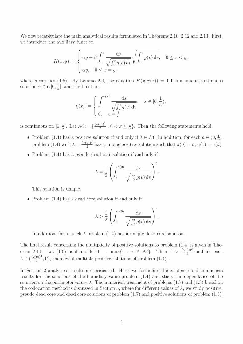
We now recapitulate the main analytical results formulated in Theorems 2.10, 2.12 and 2.13. First,we introduce the auxiliary function

H(x, y) :=

αy + β

∫ y

x

ds√

∫ s

xg(v) dv

√

∫ y

x

g(v) dv, 0 ≤ x < y,

αy, 0 ≤ x = y,

where g satisfies (1.5). By Lemma 2.2, the equation H(x, γ(x)) = 1 has a unique continuoussolution γ ∈ C[0, 1

α], and the function

χ(x) :=

∫ γ(x)

x

ds√

∫ s

xg(v) dv

, x ∈ [0,1

α),

0, x = 1α

is continuous on [0, 1α]. Let M := (χ(x))2

2: 0 < x ≤ 1

α. Then the following statements hold.

• Problem (1.4) has a positive solution if and only if λ ∈ M. In addition, for each a ∈ (0, 1α],

problem (1.4) with λ = (χ(a))2

2has a unique positive solution such that u(0) = a, u(1) = γ(a).

• Problem (1.4) has a pseudo dead core solution if and only if

λ =1

2

∫ γ(0)

0

ds√

∫ s

0g(v) dv

2

.

This solution is unique.

• Problem (1.4) has a dead core solution if and only if

λ >1

2

∫ γ(0)

0

ds√

∫ s

0g(v) dv

2

.

In addition, for all such λ problem (1.4) has a unique dead core solution.

The final result concerning the multiplicity of positive solutions to problem (1.4) is given in The-

orem 2.11. Let (1.6) hold and let Γ := maxτ : τ ∈ M. Then Γ > (χ(0))2

2and for each

λ ∈ ( (χ(0))2

2, Γ), there exist multiple positive solutions of problem (1.4).

In Section 2 analytical results are presented. Here, we formulate the existence and uniquenessresults for the solutions of the boundary value problem (1.4) and study the dependance of thesolution on the parameter values λ. The numerical treatment of problems (1.7) and (1.3) based onthe collocation method is discussed in Section 3, where for different values of λ, we study positive,pseudo dead core and dead core solutions of problem (1.7) and positive solutions of problem (1.3).

4

2 Analytical results

2.1 Auxiliary functions

Let assumption (1.5) hold, and let us introduce auxiliary functions ϕa, H and h as

ϕa(x) :=

∫ x

a

ds√

∫ s

ag(v) dv

, x ∈ (a,∞),

0, x = a,

(2.1)

where a ∈ [0,∞),

H(x, y) :=

αy + β

∫ y

x

ds√

∫ s

xg(v) dv

√

∫ y

x

g(v) dv, 0 ≤ x < y,

αy, 0 ≤ x = y,

(2.2)

h(t, y) := αy +β

1 − t

∫ y

0

ds√

∫ s

0g(v) dv

√

∫ y

0

g(v) dv, (t, y) ∈ [0, 1) × (0,∞). (2.3)

Here, the positive constants α and β are identical with those used in boundary conditions (1.4b).Note that the function H is used in the analysis of positive and pseudo dead core solutions ofproblem (1.4), while the function h for its dead core solutions.

Properties of ϕa are described in the following lemma.Lemma 2.1. Let assumption (1.5) hold and let a ∈ [0,∞). Then ϕa ∈ C[a,∞) ∩ C1(a,∞), andϕa is increasing on [a,∞).

Proof. Let c be arbitrary, c > a. Then ϕa ∈ C[a, c]∩C1(a, c], and ϕa is increasing on [a, c] by [20,Lemma 2.3 (where 1 is replaced by c)]. Since c > a is arbitrary, the result immediately follows. 2

In the following lemma, we introduce functions γ and χ and discuss their properties.Lemma 2.2. Let assumption (1.5) hold. Then the following statements follow:

(i) The function H is continuous on ∆ = (x, y) ∈ R2 : 0 ≤ x ≤ y, and ∂H

∂y(x, y) > 0 for

0 ≤ x < y.

(ii) For each x ∈[

0, 1α

]

, there exists a unique γ(x) ∈[

a, 1α

]

such that

H(x, γ(x)) = 1 for x ∈[

0, 1α

]

, (2.4)

and γ ∈ C[

0, 1α

]

, γ(x) > x for x ∈[

0, 1α

)

, γ( 1α) = 1

α.

(iii) The function

χ(x) :=

∫ γ(x)

x

ds√

∫ s

xg(v) dv

, x ∈[

0,1

α

)

,

0, x = 1α,

(2.5)

is continuous on[

0, 1α

]

.

5

Proof. (i) Let us define S, P on ∆ by

S(x, y) :=

√

∫ y

x

g(v) dv,

P (x, y) :=

∫ y

x

ds√

∫ s

xg(v) dv

, 0 ≤ x < y,

0, 0 ≤ x = y.

Then S ∈ C(∆). Let x ≥ 0 and define m := ming(s) : 0 < s ≤ x + 1. Then, by (1.5), m > 0.Hence

0 <

∫ y

x

ds√

∫ s

xg(v) dv

≤ 1√m

∫ y

x

ds√s − x

= 2

√

y − x

m, y ∈ (x, x + 1],

and consequently lim(x,y)∈∆, y→x P (x, y) = 0, which means that P is continuous at (x, x). Let0 ≤ x0 < y0. We now show that P is continuous at the point (x0, y0). Let us choose an arbitraryy∗ in the interval (x0, y0). Then P (x, y) = I1(x) + I2(x, y) for x ∈ [0, y∗] and y > y∗, where

I1(x) =

∫ y∗

x

ds√

∫ s

xg(v) dv

, I2(x, y) =

∫ y

y∗

ds√

∫ s

xg(v) dv

.

Since I1 ∈ C[0, y∗] by [20, Lemma 2.1 (where 1 was replaced by y∗)], it follows that I1 is continuousat x = x0. The continuity of P at (x0, y0) now follows from the fact that I2 is continuous at thispoint. Hence P is continuous on ∆, and from H(x, y) = αy + βP (x, y)S(x, y) we concludeH ∈ C(∆). Since

∂H

∂y(x, y) = α + β +

βq(y)

2√

∫ y

xg(v) dv

∫ y

x

ds√

∫ s

xg(v) dv

, 0 ≤ x < y,

we have ∂H∂y

(x, y) > 0 for 0 ≤ x < y.

(ii) Consider the equation H(x, y) = 1, that is,

αy + β

∫ y

x

ds√

∫ s

xg(v) dv

√

∫ y

x

g(v) dv = 1.

The function H(x, ·) is increasing on [x,∞), H(

1α, 1

α

)

= 1, and, for x ∈[

0, 1α

)

, H(

x, 1α

)

> 1.Hence, for each x ∈ [0, 1

α], there exists a unique γ(x) such that H(x, γ(x)) = 1 and γ( 1

α) = 1

α.

Clearly, γ(x) > x for x ∈ [0, 1α). In order to prove that γ ∈ C[0, 1

α], suppose the contrary, that

is suppose that γ is discontinuous at a point x = x0, x0 ∈ [0, 1α]. Then there exist sequences

νn, µn in [0, 1α] such that limn→∞ νn = x0 = limn→∞ µn, and the sequences γ(νn), γ(µn)

are convergent, limn→∞ γ(νn) = c1, limn→∞ γ(µn) = c2, c1 6= c2. Let n → ∞ in H(νn, γ(νn)) = 1and in H(µn, γ(µn)) = 1. This means H(x0, cj) = 1, j = 1, 2 and c1 = c2 = γ(x0) by the definitionof the function γ, which contradicts c1 6= c2.

(iii) By (ii),

αγ(x) + βχ(x)

√

∫ γ(x)

x

g(v) dv = 1, x ∈[

0,1

α

)

,

6

γ ∈ C[0, 1α] and γ(x) > x for x ∈ [0, 1

α). Hence, the function

√

∫ γ(x)

xg(v) dv is continuous on [0, 1

α]

and positive on [0, 1α). From

χ(x) =1 − αγ(x)

β

√

∫ γ(x)

xg(v) dv

, x ∈ [0,1

α),

we now deduce that χ ∈ C[0, 1α). Since

χ(x) ≤ 1√m

∫ γ(x)

x

ds√s − x

= 2

√

γ(x) − x

m, x ∈ [0,

1

α),

where m := ming(u) : 0 < u ≤ 1α > 0, and χ > 0 on [0, 1

α), γ( 1

α) = 1

α, we conclude

limx→( 1

α)− χ(x) = 0. Hence χ is continuous at x = 1

α, and consequently γ ∈ C[1, 1

α]. 2

Let γ be the function from Lemma 2.2(ii) defined on the interval [0, 1α] . From now on, Λ denotes

the value of γ at x = 0, that is,Λ = γ(0).

In the following lemma, we prove a property of χ which is crucial for discussing multiple positivesolutions of problem (1.4).Lemma 2.3. Let assumption (1.6) hold and let the function χ be given by (2.5). Then there existsε > 0 such that

χ(x) > χ(0) for x ∈ (0, ε). (2.6)

Proof. Note that χ(0) =∫ Λ

0

(

1/√

∫ s

0g(v) dv

)

ds. We deduce from [20, Lemma 2.2 (with 1

replaced by Λ)] that there exists an ε > 0 such that∫ Λ

x

ds√

∫ s

xg(v) dv

> χ(0) for x ∈ (0, ε). (2.7)

If γ(x) > Λ for some x ∈ (0, ε), then (2.7) yields

χ(x) =

∫ γ(x)

x

ds√

∫ s

xg(v) dv

>

∫ Λ

x

ds√

∫ s

xg(v) dv

> χ(0).

Consequently, inequality (2.6) holds for such an x. If the statement of the lemma were false, thensome x∗ ∈ (0, ε) would exist such that γ(x∗) ≤ Λ and

χ(x∗) ≤ χ(0). (2.8)

From the following equalities, cf. (2.4),

1 = αΛ + βχ(0)

√

∫ Λ

0

g(v) dv,

1 = αγ(x∗) + βχ(x∗)

√

∫ γ(x∗)

x∗

g(v) dv,

7

and from γ(x∗) ≤ Λ, we conclude that

χ(x∗) ≥ χ(0)

√

∫ Λ

0

g(v) dv/

∫ γ(x∗)

x∗

g(v) dv.

Finally, from∫ Λ

0

g(v) dv >

∫ γ(x∗)

x∗

g(v) dv

we have χ(x∗) > χ(0), which contradicts (2.8). 2

In order to discuss dead core solutions of problem (1.4) and their dead cores, we need to introducetwo additional functions µ and p related to h and study their properties.Lemma 2.4. Assume that (1.5) holds and let h be given by (2.3). Then for each t ∈ [0, 1), thereexists a unique µ(t) ∈ (0, 1

α) such that

h(t, µ(t)) = 1 for t ∈ [0, 1). (2.9)

The function µ is continuous and decreasing on [0, 1), and the function

p(t) :=1

1 − t

∫ µ(t)

0

ds√

∫ s

0g(v) dv

, t ∈ [0, 1), (2.10)

is continuous and increasing on [0, 1). Moreover, limt→1− p(t) = ∞.

Proof. It follows from (1.5) that h ∈ C([0, 1) × (0,∞)). Also, h is increasing w.r.t. both vari-ables, limt→1− h(t, y) = ∞ for any y ∈ (0, 1

α], and limy→0+ h(t, y) = 0, limy→ 1

αh(t, y) > 1 for any

t ∈ [0, 1). Hence, for each t ∈ [0, 1), there exists a unique µ(t) ∈ (0, 1α) such that h(t, µ(t)) = 1.

In order to prove that µ is decreasing on [0, 1) assume on the contrary that µ(t1) ≤ µ(t2) forsome 0 ≤ t1 < t2 < 1. Then h(t1, µ(t1)) < h(t2, µ(t2)) which contradicts h(tj, µ(tj)) = 1 forj = 1, 2. Hence, µ is decreasing on [0, 1). If µ was discontinuous at a point t0 ∈ [0, 1), then therewould exist sequences νn, τn in [0, 1) such that limn→∞ νn = t0 = limn→∞ τn and µ(νn),µ(τn) are convergent, limn→∞ µ(νn) = c1, limn→∞ µ(τn) = c2 with c1 6= c2. Taking the limitsn → ∞ in h(νn, µ(νn)) = 1 and h(τn, µ(τn)) = 1, we obtain h(t0, cj) = 1, j = 1, 2. Consequently,c1 = c2 = µ(x0) by the definition of the function µ, which is not possible.

By (2.9),

αµ(t) +β

1 − t

∫ µ(t)

0

ds√

∫ s

0g(v) dv

√

∫ µ(t)

0

g(v) dv = 1 for t ∈ [0, 1),

and therefore

p(t) =1 − αµ(t)

β

√

∫ µ(t)

0g(v) dv

, t ∈ [0, 1). (2.11)

It follows from the properties of µ that the functions 1 − αµ(t), 1/

√

∫ µ(t)

0g(v) dv are continuous,

positive and increasing on [0, 1). Hence (2.11) implies that p ∈ C[0, 1) and p is increasing.

Moreover, limt→1− p(t) = ∞ since∫ µ(t)

0(1/√

∫ s

0g(v) dv) ds is bounded on [0, 1). 2

8

Corollary 2.5. Let assumption (1.5) hold. Then

1

1 − t

∫ µ(t)

0

ds√

∫ s

0g(v) dv

>

∫ Λ

0

ds√

∫ s

0g(v) dv

for t ∈ (0, 1), (2.12)

and for each λ satisfying the inequality

λ >1

2

∫ Λ

0

ds√

∫ s

0g(v) dv

2

, (2.13)

there exists a unique ρ ∈ (0, 1) such that

∫ µ(ρ)

0

ds√

∫ s

0g(v) dv

= (1 − ρ)√

2λ. (2.14)

Proof. The equalities h(0, y) = H(0, y) for y ∈ (0,∞) and H(0, Λ) = 1 imply that µ(0) = Λ. Sincethe function p defined by (2.10) is continuous and increasing on [0, 1), it follows p(t) > p(0) fort ∈ (0, 1), see (2.12). Let us choose an arbitrary λ satisfying (2.13). Then

√2λ > p(0). Now, the

properties of p guarantee that equation√

2λ = p(t) has a unique solution ρ ∈ (0, 1). This means,that (2.14) holds for a unique ρ ∈ (0, 1). 2

2.2 Dependence of solutions on the parameter λ

The following two lemmas characterize the dependence of positive and dead core solutions ofproblem (1.4) on the parameter λ.Lemma 2.6. Let assumption (1.5) hold and let u be a positive solution of problem (1.4) for someλ > 0. Also, let a := minu(t) : 0 ≤ t ≤ 1, and Q := maxu(t) : 0 ≤ t ≤ 1. Then a = u(0),Q = u(1),

∫ Q

a

ds√

∫ s

ag(v) dv

=√

2λ, (2.15)

∫ u(t)

a

ds√

∫ s

ag(v) dv

=√

2λt for t ∈ [0, 1], (2.16)

andH(a,Q) = 1, (2.17)

where the function H is given by (2.2).

Proof. Since u′(0) = 0 and u′′(t) = λg(u(t)) > 0 for t ∈ [0, 1], we conclude that u′ > 0 on (0, 1]and a = u(0), Q = u(1). By integrating the equality u′′(t)u′(t) = λg(u(t))u′(t) over [0, t] ⊂ [0, 1],we obtain

(u′(t))2 = 2λ

∫ u(t)

a

g(v) dv,

9

and consequently, since u′ > 0 on (0, 1],

u′(t) =√

2λ

√

∫ u(t)

a

g(v) dv, t ∈ [0, 1].

Finally, integratingu′(t)

√

∫ u(t)

ag(v) dv

=√

2λ, t ∈ (0, 1],

over [0, t] yields (2.16). Now we set t = 1 in (2.16) and obtain (2.15). Equality (2.17) follows fromαu(1) + βu′(1) = 1 and from

u(1) = Q, u′(1) =√

2λ

√

∫ Q

a

g(v) dv =

∫ Q

a

ds√

∫ s

ag(v) dv

√

∫ Q

a

g(v) dv.

2

Remark 2.7. Let (1.5) hold and let u be a pseudo dead core solution of problem (1.4). Then, bythe definition of pseudo dead core solutions, u(0) = 0. We can proceed analogously to the proofof Lemma 2.6 in order to show that

∫ Q

0

ds√

∫ s

ag(v) dv

=√

2λ, (2.18)

where Q = u(1), and

∫ u(t)

0

ds√

∫ s

ag(v) dv

=√

2λt for t ∈ [0, 1], (2.19)

H(0, Q) = 1. (2.20)

From (2.20), we finally have Q = Λ. Consequently, u(1) = Λ.Remark 2.8. If λ = 0, then u(t) = 1

α, t ∈ [0, 1], is the unique solution of problem (1.4). This

solution is positive.Lemma 2.9. Let assumption (1.5) hold and let u be a dead core solution of problem (1.4) forsome λ = λ0. Moreover, let Q := maxu(t) : 0 ≤ t ≤ 1. Then Q = u(1) and there exists a pointρ ∈ (0, 1) such that u(t) = 0 for t ∈ [0, ρ],

∫ u(t)

0

ds√

∫ s

0g(v) dv

=√

2λ0(t − ρ) for t ∈ [ρ, 1], (2.21)

∫ Q

0

ds√

∫ s

0g(v) dv

=√

2λ0(1 − ρ), (2.22)

andh(ρ,Q) = 1, (2.23)

where the function h is given by (2.3). Furthermore, u is the unique dead core solution of problem(1.4) with λ = λ0.

10

Proof. Since u is a dead core solution of problem (1.4) with λ = λ0, there exists by definition,a point ρ ∈ (0, 1) such that u ∈ C1[0, 1] ∩ C2(ρ, 1], u(t) = 0 for t ∈ [0, ρ] and u > 0 on (ρ, 1].Consequently, u′ > 0 on (ρ, 1], and Q = u(1). We can now proceed analogously to the proof ofLemma 2.6 to show that

u′(t) =√

2λ0

√

∫ u(t)

0

g(v) dv, t ∈ [ρ, 1],

and (2.21) hold. Setting t = 1 in (2.21), we obtain (2.22). Also, from (1.4b), u(1) = Q,

u′(1) =√

2λ0

√

∫ Q

0

g(v) dv =1

1 − ρ

∫ Q

0

ds√

∫ s

0g(v) dv

√

∫ Q

0

g(v) dv,

(2.23) follows.

It remains to verify that u is the unique dead core solution of problem (1.4) with λ = λ0. Let ussuppose that w is another dead core solution of the above problem. Let w(t) = 0 for t ∈ [0, ρ1] andw > 0 on (ρ1, 1] for some ρ1 ∈ (0, 1). Then w′′(t) = λ0g(w(t)) > 0 for t ∈ (ρ1, 1], and consequentlyw′ > 0 on (ρ1, 1] and Q1 := maxw(t) : 0 ≤ t ≤ 1 = w(1). Hence, cf. (2.22) and (2.23),

∫ Q1

0

ds√

∫ s

0g(v) dv

=√

2λ0(1 − ρ1), (2.24)

αQ1 + β√

2λ0

√

∫ Q1

0

g(v) dv = 1. (2.25)

Since

αQ + β√

2λ0

√

∫ Q

0

g(v) dv = 1 (2.26)

by (2.23), and the function p(r) := αr+β√

2λ0

√

∫ r

0g(v) dv is increasing and continuous on (0,∞),

we deduce from (2.25) and (2.26) that Q = Q1. Then (2.22) and (2.24) yield ρ = ρ1. Therefore,∫ w(t)

0

(

1/√

∫ s

0g(v) dv

)

ds =√

2λ0(t − ρ) for t ∈ [ρ, 1]. Finally, since w(t) = 0 for t ∈ [0, ρ] and

since by Lemma 2.1 the function ϕ0 is increasing on [0,∞), u = w follows. This completes theproof. 2

2.3 Main results

Let the function χ be given by (2.5) and let us denote by M the range of the function χ2

2restricted

to the interval (0, 1α],

M :=

(χ(x))2

2: 0 < x ≤ 1

α

.

Since χ ∈ C[0, 1α] by Lemma 2.2(iii), χ(x) > 0 for x ∈ [0, 1

α) and χ( 1

α) = 0, we can have either

(i) χ(x) < χ(0) for x ∈ (0, 1α], or (ii) χ(x1) ≥ χ(0) for some x1 ∈ (0, 1

α]. For (i), we have

M = [0, (χ(0))2

2), while in case of (ii), M = [0, Γ] with

Γ := maxτ : τ ∈ M (2.27)

11

holds. Clearly, Γ ≥ (χ(0))2

2.

Positive solutions of problem (1.4) are analyzed in the following theorem.Theorem 2.10. Let assumption (1.5) hold. Then problem (1.4) has a positive solution if and only

if λ ∈ M. Additionally, for each a ∈ (0, 1α], problem (1.4) with λ = (χ(a))2

2has a unique positive

solution u such that u(0) = a and u(1) = γ(a).

Proof. Let u be a positive solution of problem (1.4) for λ > 0. By Lemma 2.6, (2.17) holds witha = u(0) > 0 and Q = u(1). Furthermore, by Lemmas 2.2(ii) and 2.6, Q = γ(a), which togetherwith (2.15) implies that

√2λ = χ(a). Consequently, λ ∈ M. For λ = 0, problem (1.4) has the

unique positive solution u = 1α, see Remark 2.8. Since χ( 1

α) = 0, 0 ∈ M. Consequently, if problem

(1.4) has a positive solution, then λ ∈ M.

We now show that for each λ ∈ M, problem (1.4) has a positive solution, and if λ = (χ(a))2

2

for some a ∈ (0, 1α], then problem (1.4) has a unique positive solution u such that u(0) = a and

u(1) = γ(a). Let us choose λ ∈ M. Then√

2λ = χ(a) for some a ∈ (0, 1α]. If a = 1

α, then χ(a) = 0.

Consequently, λ = 0 and u = 1α

is the unique solution of problem (1.4). Clearly, u(0) = a andu(1) = γ(a) since a = γ(a) = 1

α. Let us suppose that a ∈ (0, 1

α). If u is a positive solution of

problem (1.4) and u(0) = a, then, by Lemma 2.6, see (2.16), the equality ϕa(u(t)) =√

2λt holds

for t ∈ [0, 1], where ϕa is given by (2.1). Hence, in order to prove that for λ = (χ(a))2

2problem

(1.4) has a unique positive solution u such that u(0) = a and u(1) = γ(a), we have to show thatthe equation

ϕa(u(t)) =√

2λt, t ∈ [0, 1]. (2.28)

has a unique solution u, this solution is a positive solution of problem (1.4), and u(0) = a,u(1) = γ(a). Since ϕa ∈ C[a,∞)∩C1(a,∞), ϕa is increasing by Lemma 2.1, and ϕa(γ(a)) = χ(a),equation (2.28) has a unique solution u ∈ C[0, 1]. It follows from ϕa(a) = 0 and ϕa(u(1)) =√

2λ = χ(a) that u(a) = a and u(1) = γ(a). In addition,

u′(t) =

√2λ

ϕ′a(u(t))

=

√

2λ

∫ u(t)

a

g(v) dv, t ∈ (0, 1]. (2.29)

Hence, u ∈ C1(0, 1] and limt→0+ u′(t) = 0. In order to show that u′ is continuous at t = 0, we setM = maxg(s) : a ≤ s ≤ 1

α > 0. Then, cf. (2.28),

√2λt =

∫ u(t)

a

ds√

∫ s

ag(v) dv

≥ 1√M

∫ u(t)

a

ds√s − a

= 2

√

u(t) − a

M,

and therefore,

0 <u(t) − u(0)

t=

u(t) − a

t≤ Mλt

2, t ∈ (0, 1].

Consequently, u′(0) = limt→0+u(t)−a

t= 0, and so u′ is continuous at t = 0, or equivalently,

u ∈ C1[0, 1]. Now (2.29) indicates that u ∈ C2(0, 1] and

u′′(t) =√

2λg(u(t))u′(t)

2

√

∫ u(t)

ag(v) dv

= λg(u(t)) for t ∈ (0, 1].

12

Moreover, by the de L’Hospital rule,

limt→0+

u′(t) − u′(0)

t= lim

t→0+

u′(t)

t= lim

t→0+

1

t

√

2λ

∫ u(t)

a

g(v) dv

=√

2λ limt→0+

g(u(t))u′(t)

2

√

∫ u(t)

ag(v) dv

= λ limt→0+

g(u(t))

= λg(u(0)).

As a result u ∈ C2[0, 1] and u′′(t) = λg(u(t)) for t ∈ [0, 1]. Since u(1) = γ(a) and, by (2.29),

u′(1) = χ(a)

√

∫ γ(a)

ag(v) dv, we have

αu(1) + βu′(1) = αγ(a) + β

∫ γ(a)

a

ds√

∫ s

ag(v) dv

√

∫ γ(a)

a

g(v) dv = H(a, γ(a)) = 1

by Lemma 2.2(ii). Thus, u satisfies (1.4b), and therefore u is a unique positive solution of problem(1.4) such that u(0) = a and u(1) = γ(a). 2

The following theorem deals with multiple positive solutions of problem (1.4).

Theorem 2.11. Let assumption (1.6) hold. Then Γ > (χ(0))2

2, with Γ given by (2.27), and for each

λ ∈ ( (χ(0))2

2, Γ), there exist multiple positive solutions of problem (1.4).

Proof. By Lemmas 2.2(iii) and 2.3, χ ∈ C[0, 1α], χ( 1

α) = 0, and χ(x) > χ(0) in a right neighbour-

hood of x = 0. Hence, Γ > (χ(0))2

2. Let us choose λ ∈ ( (χ(0))2

2, Γ). Then there exist 0 < x1 < x2 < 1

α

such that λ =(χ(xj))

2

2for j = 1, 2. Now Theorem 2.10 guarantees that problem (1.4) has positive

solutions u1 and u2 such that uj(0) = xj, j = 1, 2. Since x1 6= x2, we have u1 6= u2 and therefore,

for each λ ∈ ( (χ(0))2

2, Γ), problem (1.4) has multiple positive solutions. 2

Next, we present results for pseudo dead core solutions of problem (1.4). Note that here Λ = γ(0).Theorem 2.12. Let assumption (1.5) hold. Then problem (1.4) has a pseudo dead core solutionif and only if

λ =1

2

∫ Λ

0

ds√

∫ s

0g(v) dv

2

. (2.30)

Moreover, for λ given by (2.30), problem (1.4) has a unique pseudo dead core solution such thatu(1) = Λ.

Proof. Let us assume that u is a pseudo dead core solution of problem (1.4) and let Q := u(1).Then, by Remark 2.7, equalities (2.18), (2.20) hold, and Q = Λ. Also, (2.19) implies that u is asolution of the equation

ϕ0(u(t)) =√

2λt, t ∈ [0, 1], (2.31)

where ϕ0 and λ are given by (2.1) and (2.30), respectively. The result follows by showing thatequation (2.31) has a unique solution and that this solution is a pseudo dead core solution of prob-lem (1.4). We verify these facts for solutions of (2.31) arguing as in the proof of Theorem 2.10,

13

with a replaced by 0. 2

In the final theorem below, we deal with dead core solutions of problem (1.4).Theorem 2.13. Let assumption (1.5) hold and let µ be the function defined in Lemma 2.4. Thenthe following statements hold:

(i) Problem (1.4) has a dead core solution if and only if

λ >1

2

∫ Λ

0

ds√

∫ s

0g(v) dv

2

. (2.32)

(ii) For each λ satisfying (2.32), problem (1.4) has a unique dead core solution.

(iii) If the subinterval [0, ρ] is the dead core of a dead core solution u of problem (1.4), thenmaxu(t) : 0 ≤ t ≤ 1 = µ(ρ) and

∫ µ(ρ)

0

ds√

∫ s

0g(v) dv

= (1 − ρ)√

2λ. (2.33)

Proof. (i) Let u be a dead core solution of problem (1.4) for some λ = λ0 and let Q := u(1). Thenthere exists a point ρ ∈ (0, 1) such that u(t) = 0 for t ∈ [0, ρ], and equalities (2.21), (2.22) and(2.23) are satisfied by Lemma 2.9. We deduce from (2.23) and from Lemma 2.4 that Q = µ(ρ).Therefore, cf. (2.22),

1

1 − ρ

∫ µ(ρ)

0

ds√

∫ s

0g(v) dv

=√

2λ0.

Since1

1 − ρ

∫ µ(ρ)

0

ds√

∫ s

0g(v) dv

>

∫ Λ

0

ds√

∫ s

0g(v) dv

by Corollary 2.5, we have

λ0 >1

2

∫ Λ

0

ds√

∫ s

0g(v) dv

2

.

Hence, if problem (1.4) has a dead core solution, then λ satisfies inequality (2.32).

We now prove that for each λ satisfying (2.32), problem (1.4) has a dead core solution. Let uschoose λ satisfying (2.32). Then, by Corollary 2.5, there exists a unique ρ ∈ (0, 1) such that

∫ µ(ρ)

0

ds√

∫ s

0g(v) dv

= (1 − ρ)√

2λ. (2.34)

Let us now consider, cf. (2.21),

ϕ0(w(t)) = (t − ρ)√

2λ, t ∈ [ρ, 1], (2.35)

14

where ϕ0 is given by (2.1). Since ϕ0 ∈ C[0,∞) ∩ C1(0,∞) and ϕ0 is increasing on [0,∞) byLemma 2.1, ϕ0(0) = 0, and, by (2.34), ϕ0(µ(ρ)) = (1 − ρ)

√2λ, there exists a unique solution

w ∈ C[ρ, 1] of (2.35) and w(ρ) = 0, w(1) = µ(ρ). In addition,

w′(t) =

√2λ

ϕ′0(w(t))

=

√

2λ

∫ w(t)

0

g(v) dv, t ∈ (ρ, 1],

and consequently, w ∈ C1(ρ, 1] and limt→ρ+ w′(t) = 0. Since

(t − ρ)√

2λ =

∫ w(t)

0

ds√

∫ s

0g(v) dv

=w(t)

√

∫ ξ(t)

0g(v) dv

, t ∈ (ρ, 1],

by the Mean Value Theorem for integrals, where 0 < ξ(t) < w(t), we have

w(t) − w(ρ)

t − ρ=

w(t)

t − ρ=

√

2λ

∫ ξ(t)

0

g(v) dv.

Therefore,

limt→ρ+

w(t) − w(ρ)

t − ρ= lim

t→ρ+

√

2λ

∫ ξ(t)

0

g(v) dv = 0

since limt→ρ+ ξ(t) = 0. Hence, w′ is continuous at t = ρ, and w ∈ C1[ρ, 1]. Furthermore,

w′′(t) =

√2λg(w(t))w′(t)

2

√

∫ w(t)

0g(v) dv

= λg(w(t)), t ∈ (ρ, 1].

Let

u(t) :=

0 for t ∈ [0, ρ),

w(t) for t ∈ [ρ, 1].

Then u ∈ C1[0, 1] ∩ C2(ρ, 1], u′′(t) = λg(u(t)) for t ∈ (ρ, 1], u(ρ) = u′(ρ) = 0, u(1) = µ(ρ), and

u′(1) =

√

2λ

∫ u(1)

0

g(v) dv =1

1 − ρ

∫ µ(ρ)

0

ds√

∫ s

0g(v) dv

√

∫ µ(ρ)

0

g(v) dv.

Thus,

αu(1) + βu′(1) = αµ(ρ) +β

1 − ρ

∫ µ(ρ)

0

ds√

∫ s

0g(v) dv

√

∫ µ(ρ)

0

g(v) dv = h(ρ, µ(ρ)),

where h is given by (2.3). Since h(ρ, µ(ρ)) = 1 by Lemma 2.4, u satisfies the boundary conditions(1.4b). Consequently, u is a dead core solution of problem (1.4).(ii) Let us choose an arbitrary λ satisfying (2.32). By (i), problem (1.4) has a dead core solutionwhich is unique by Lemma 2.9.(iii) Let the subinterval [0, ρ] be the dead core of a dead core solution u of problem (1.4). Then, byLemma 2.9, equalities (2.22) and (2.23) hold with λ0 replaced by λ and Q = maxu(t) : 0 ≤ t ≤ 1.

15

Since h(ρ, µ(ρ)) = 1 by the definition of the function µ, we have µ(ρ) = Q. Equality (2.33) nowfollows from (2.22) with Q and λ0 replaced by µ(ρ) and λ, respectively. 2

Example 2.14. We now turn to the case study of the boundary value problem (1.7),

u′′(t) =λ

√

u(t), u′(0) = 0, αu(1) + βu′(1) = 1, α > 0, β > 0.

Note that (1.7) is a special case of (1.4) with g(u) = 1√u

satisfying (1.6). Since∫ y

x

ds√

∫ s

x(1/

√v) dv

=4

3√

2

√√y −

√x(√

y + 2√

x)

, 0 ≤ x < y,

we have

H(x, y) = αy + β

∫ y

x

ds√

∫ s

x(1/

√v) dv

√

∫ y

x

dv√v

= αy +4β

3(√

y −√

x)(√

y + 2√

x)

for 0 ≤ x < y, and H(x, x) = αx for x ≥ 0. By Lemma 2.2, the equation H(x, y) = 1 has a uniquesolution y = γ(x) for x ∈ [0, 1

α], γ ∈ C[0, 1

α], γ(x) > x for x ∈ [0, 1

α), and γ( 1

α) = 1

α. Let

k(x) :=x

γ(x)for x ∈ [0, 1

α]. (2.36)

Then k ∈ C[0, 1α], k(0) = 0, and k( 1

α) = 1. In order to show that k is increasing on [0, 1

α] it is

sufficient to verify that k is injective. Let us assume that this is not the case, then there existx1, x2 ∈ [0, 1

α], x1 6= x2, such that k(x1) = k(x2). From H(xj, γ(xj)) = 1, j = 1, 2, or equivalently,

from

3α + 4β(

1 −√

k(xj))(

1 + 2√

k(xj))

=3

γ(xj), j = 1, 2,

it follows that γ(x1) = γ(x2), and x1 = x2, which is a contradiction. Hence, k is increasing on[0, 1

α] and therefore, there exists the inverse function k−1 mapping [0, 1] onto [0, 1

α]. Since

H(k(x)γ(x), γ(x)) = γ(x)

[

α +4β

3

(

1 −√

k(x))(

1 + 2√

k(x))

]

and H(k(x)γ(x), γ(x)) = 1 for x ∈ [0, 1α], we have

γ(x) =3

3α + 4β(

1 −√

k(x))(

1 + 2√

k(x)) .

Consequently,

(χ(x))2 =

∫ γ(x)

x

ds√

∫ s

x(1/

√v) dv

2

=8

9

(

√

γ(x) −√

x)(

√

γ(x) + 2√

x)2

=8

9(γ(x))

3

2

(

1 −√

k(x))(

1 + 2√

k(x))2

=8

9

3

3α + 4β(

1 −√

k(x))(

1 + 2√

k(x))

3

2(

1 −√

k(x))(

1 + 2√

k(x))2

.

16

In order to discuss the range M of the function χ2

2and the value of (χ(x))2

2for x ∈ [0, 1

α], we first

consider properties of the function

δ(x) :=4

9

3

3α + 4β(

1 −√x)(

1 + 2√

x)

3

2(

1 −√

x)(

1 + 2√

x)2

(2.37)

defined on [0, 1]. Let

f(x) := δ((x − 1

2

)2)

for x ∈ [1, 3].

Then

f(x) =2

9

(

3

3α + 2βx(3 − x)

) 3

2

x2(3 − x),

f ′(x) =2x

3

(

3

3α + 2βx(3 − x)

) 3

2 p(x)

3α + 2βx(3 − x),

where p(x) = 6α + 3(β − α)x − βx2. The function p vanishes only at point

x∗ =1

2β

(

3(β − α) +√

9(β − α)2 + 24αβ)

in the interval [1, 3], and 2 < x∗ < 3, because p(2) > 0 and p(3) < 0. Since f ′(x∗) = 0, p > 0 on[1, x∗), p < 0 on (x∗, 3] and

2x

3

(

3

3α + 2βx(3 − x)

) 3

2 1

3α + 2βx(3 − x)> 0

for x ∈ [1, 3], we have f ′ > 0 on [1, x∗) and f ′ < 0 on (x∗, 3]. Let us define k∗ := (x∗−12

)2.Then k∗ ∈ (1

4, 1), and it follows from f ′(x) = x−1

2δ′((x−1

2)2) that δ′ > 0 on (0, k∗) and δ′ < 0

on (k∗, 1]. Consequently, δ is increasing on [0, k∗] and decreasing on [k∗, 1]. It follows from theequality (χ(x))2 = 2δ(k(x)) for x ∈ [0, 1

α] and from the properties of the functions δ and k

that χ2 is increasing on [0, k−1(k∗)] and decreasing on [k−1(k∗),1α]. Hence, M = [0,M ], where

M := maxδ(x) : 0 ≤ x ≤ 1. Also,

(χ(0))2 =8

9

(

3

3α + 4β

) 3

2

, χ(1) = 0.

Using properties of the function χ and the results of Theorems 2.10–2.13, we can now characterizethe structure of the solution u:(i) For each λ > (M,∞), there exists only a unique dead core solution of problem (1.7).(ii) For λ = M , there exists a unique dead core solution and a unique positive solution of problem(1.7).

(iii) For each λ ∈(

49

(

33α+4β

) 3

2

,M)

, there exists a unique dead core solution and exactly two

positive solutions of problem (1.7).

(iv) For λ = 49

(

33α+4β

) 3

2

there exists the unique pseudo dead core solution u(t) = 33α+4β

t4

3 and a

unique positive solution of problem (1.7).

17

(v) For each λ ∈[

0, 49

(

33α+4β

) 3

2)

, there exists only a unique positive solution of problem (1.7).

Using Theorem 2.10, Lemma 2.6 and the properties of the function δ, we can specify furtherproperties of positive solutions of problem (1.7):

(i) If u is the (unique) positive solution of problem (1.7) with λ ∈[

0, 49

(

33α+4β

) 3

2)

∪ M, then

u(0) = x0u(1), where x0 6= 0 is the root of the equation δ(x) − λ = 0.

(ii) If u1, u2 are the (unique) positive solutions of problem (1.7) with λ ∈(

49

(

33α+4β

) 3

2

,M)

, then

uj(0) = xjuj(1), j=1,2, where 0 < x1 < k∗ < x2 < 1, are the roots of the equation δ(x) − λ = 0.

We are also able to give some more information on the dead core solutions of problem (1.7). Since

h(t, y) = αy +β

1 − t

∫ y

0

ds√

∫ s

0(1/

√v) dv

√

∫ y

0

dv√v

= αy +4βy

3(1 − t),

the function µ(t) = 3(1−t)3α(1−t)+4β

, t ∈ [0, 1), is the solution of the equation h(t, y) = 1. Let us choose

an arbitrary λ > 49

(

33α+4β

) 3

2

. By Corollary 2.5 the equation, see (2.14),

4

3√

2

(

3(1 − t)

3α(1 − t) + 4β

) 3

4

= (1 − t)√

2λ, t ∈ [0, 1),

has a unique solution ρ ∈ (0, 1). Consequently,

λ =4

9√

1 − ρ

(

3

3α(1 − ρ) + 4β

) 3

2

.

One can easily show that the function

u(t) =

0 for t ∈ [0, ρ],

(3

2

√λ(t − ρ)

) 4

3

for t ∈ (ρ, 1],

is the unique dead core solution of problem (1.7). Additionally, it follows from Theorem 2.13(iii)

that maxu(t) : 0 ≤ t ≤ 1 = 3(1−ρ)3α(1−ρ)+4β

since maxu(t) : 0 ≤ t ≤ 1 = µ(ρ).

3 Numerical Treatment

We now aim at the numerical approximation to the solution of the following two-point boundaryvalue problem:

u′′(t) = f(t, u(t)), t ∈ [0, 1], (3.38a)

u′(0) = 0, βu′(1) + αu(1) = A, β ≥ 0, α, A > 0. (3.38b)

For the numerical solution of (3.38) we are using the collocation method implemented in our Mat-

lab code bvpsuite. It is a new version of the general purpose Matlab code sbvp, cf. [6], [7] and

18

[16]. This code has already been used to treat a variety of problems relevant in application, seefor example [13], [14], [15], [17], and [19]. Collocation is a widely used and well-studied standardsolution method for two-point boundary value problems, cf. [5] and the references therein. It canalso be successfully applied to boundary value problems with singularities.

In the scope of the code are systems of ordinary differential equations of arbitrary order. Forsimplicity of notation we present a problem of maximal order four which can be given in a fullyimplicit form,

F (t, u(4)(t), u(3)(t), u′′(t), u′(t), u(t)) = 0, 0 ≤ t ≤ 1, (3.39a)

b(u(3)(0), u′′(0), u′(0), u(0), u(3)(1), u′′(1), u′(1), u(1)) = 0. (3.39b)

In order to compute the numerical approximation, we first introduce a mesh

∆h := τi : i = 0, . . . , N, 0 = τ0 < τ1 · · · < τN = 1.

The approximation for u is a collocation function

p(t) := pi(t), t ∈ [τi, τi+1], i = 0, . . . , N − 1,

where we require p ∈ Cq−1[0, 1] in case that the order of the underlying differential equation is q.Here, pi are polynomials of maximal degree m− 1 + q which satisfy the system (3.40a) at m innercollocation points

ti,j = τi + ρj(τi+1 − τi), i = 0, . . . , N − 1, j = 1, . . . ,m, 0 < ρ1 < · · · < ρm < 1,

and the associated boundary conditions (3.40b).Classical theory, cf. [5], predicts that the convergence order for the global error of the methodis at least O(hm), where h is the maximal stepsize, h := maxi(τi+1 − τi). To increase efficiency,an adaptive mesh selection strategy based on an a posteriori estimate for the global error of thecollocation solution is utilized. A more detailed description of the numerical approach can befound in [20].

The code bvpsuite also allows to follow a path in the parameter-solution space. This meansthat in the following problem setting, parameter ϑ is unknown:

F (t, u(4)(t), u(3)(t), u′′(t), u′(t), u(t), ϑ) = 0, 0 ≤ t ≤ 1, (3.40a)

b(u(3)(0), u′′(0), u′(0), u(0), u(3)(1), u′′(1), u′(1), u(1)) = 0, ϑ = λ, (3.40b)

where λ is given. The pathfollowing strategy can also cope with turning points in the path. Thetheoretical justification for the pathfollowing strategy implemented in bvpsuite has been givenin [18].

We first study the boundary problem problem (1.7). Positive solutions of problem (1.3) will bediscussed in Section 3.4.The above analytical discussion indicates that depending on the values of α, β, λ, the problem hasone or more positive solutions, a pseudo dead core solution or a dead core solution. All numericalapproximations have been calculated on a fixed mesh with N = 500 subintervals and collocation

19

degree m = 4. Figure 1 shows δ(x) for our choice of parameters used in the following sections.Here, δ is given by (2.37).

0 0.2 0.4 0.6 0.8 10

0.05

0.1

0.15

0.2

0.25

x

δ(x)

0 0.2 0.4 0.6 0.8 10

0.01

0.02

0.03

0.04

0.05

0.06

x

δ(x)

Figure 1: δ(x) for α = β = 1 (left) and for α = 5, β = 0.5 (right).

3.1 Positive Solutions

For λ ∈ [0, δ(0)), δ(0) = (4/9)(3/(3α + 4β))3/2, there exists a unique positive solution. Thissolution was found numerically by using the original problem formulation (1.7). For α = β = 1we obtain δ(0) ≈ 0.12469. In Figure 2 we display the numerical solution, the error estimate andthe residual for λ = 0.05. The residual r(t) is calculated by substituting the numerical solutionp(t) into the differential equation,

r(t) := p′′(t) − λ√

p(t).

0 0.2 0.4 0.6 0.8 1

0.925

0.93

0.935

0.94

0.945

t

u(t)

Solution

0 0.2 0.4 0.6 0.8 11.5

1.6

1.7

1.8

1.9

2

2.1

2.2

2.3x 10

−12

t

e(t)

Error Estimate

0 0.2 0.4 0.6 0.8 1

10−12

t

r(t)

Residual

Figure 2: Problem (1.7): The numerical solution, the error estimate and the residual for α = 1,β = 1 and λ = 0.05.

Due to the very small size of the error estimate and residual, it is obvious that the numericalapproximation is very accurate. According to the analytical results, a solution to the problemsatisfies |u(0) − x0u(1)| = 0 where x0 is a root of δ(x) − λ = 0. Here, we have x0 = 0.972608and |u(0) − x0u(1)| = 6.4 10−8 which again shows the high quality of the numerical solution. InFigure 3 we depict the results for the parameter α = 5, β = 0.5 and λ = 0.02 < δ(0) ≈ 0.03294.For this choice of parameters x0 = 0.877692 and |u(0) − x0u(1)| = 3.5 10−8.

20

0 0.2 0.4 0.6 0.8 1

0.175

0.18

0.185

0.19

0.195

t

u(t)

Solution

0 0.2 0.4 0.6 0.8 1

0.4

0.6

0.8

1

1.2

1.4

1.6

1.8

x 10−13

t

e(t)

Error Estimate

0 0.2 0.4 0.6 0.8 1

10−14

10−13

t

r(t)

Residual

Figure 3: Problem (1.7): The numerical solution, the error estimate and the residual for α = 5,β = 0.5 and λ = 0.02.

For λ = δ(0) = (4/9)(3/(3α + 4β))3/2 there exists a unique positive solution. To compute itsnumerical approximation, we rewrite the problem (1.7) and consider

u′′(t)√

u(t) = λ =4

9

(

3

3α + 4β

) 3

2

, t ∈ [0, 1], (3.41a)

u′(0) = 0, αu(1) + βu′(1) = 1, α > 0, β > 0. (3.41b)

The numerical results related to parameter sets α = 1, β = 1, and α = 5, β = 0.5 are shown inFigure 4, and Figure 5, respectively.

0 0.2 0.4 0.6 0.8 1

0.8

0.81

0.82

0.83

0.84

0.85

0.86

t

u(t)

Solution

0 0.2 0.4 0.6 0.8 1

1.5

1.6

1.7

1.8

1.9

2

2.1

2.2

x 10−11

t

e(t)

Error Estimate

0 0.2 0.4 0.6 0.8 1

10−11

t

r(t)

Residual

Figure 4: Problem (3.41): The numerical solution, the error estimate and the residual for α = 1,

β = 1 and λ = (4/9)(3/(3α + 4β))3/2.

Again, the error estimate and the residual are both very small and x0 = 0.919315, so |u(0) −x0u(1)| = 3.5 10−7.

21

0 0.2 0.4 0.6 0.8 1

0.155

0.16

0.165

0.17

0.175

0.18

0.185

0.19

t

u(t)

Solution

0 0.2 0.4 0.6 0.8 1

0.4

0.6

0.8

1

1.2

1.4

1.6

1.8

2

x 10−12

t

e(t)

Error Estimate

0 0.2 0.4 0.6 0.8 1

10−13

10−12

t

r(t)

Residual


β = 0.5 and λ = (4/9)(3/(3α + 4β))3/2.

Moreover, x0 = 0.783283 and |u(0) − x0u(1)| = 1.7 10−8.

For λ ∈ (δ(0),M) with M = maxδ(x) : 0 ≤ x ≤ 1 there exist two positive solutions. These twodifferent solutions for a fixed value of λ can be characterized via the roots x1,2 of δ(x) − λ = 0for x ∈ [0, 1]. The choice of parameters remains the same. For α = 1, β = 1 and λ = 0.15the solution corresponding to x1 ≈ 0.009159 is shown in Figure 6. The solution corresponding tox2 ≈ 0.896054 is depicted in Figure 7. Note that for these values of α and β we have M ≈ 0.28049.

The first of those two solutions was found using the reformulated problem (3.41) with λ as theright hand side. For the second solution it was necessary to rewrite the problem again and use

u′′(t)√

u(t) =4

9

(

3

3α + 4β(1 −√x)(1 + 2

√x)

) 3

2

(1 −√

x)(1 + 2√

x)2, t ∈ [0, 1],(3.42a)

u′(0) = 0, αu(1) + βu′(1) = 1, α > 0, β > 0, (3.42b)

with x as a free unknown parameter and x = x2 as a necessary additional boundary condition.

0 0.2 0.4 0.6 0.8 1

0.05

0.1

0.15

0.2

0.25

0.3

0.35

0.4

t

u(t)

Solution

0 0.2 0.4 0.6 0.8 1

1

2

3

4

5

6

7

8x 10

−15

t

e(t)

Error Estimate

0 0.2 0.4 0.6 0.8 1

10−12

10−10

t

r(t)

Residual

Figure 6: Problem (3.41): The numerical solution, the error estimate and the residual for α = 1,β = 1 and λ = 0.15. The associated root is x1.

Here, x1 = 0.009159 and |u(0) − x1u(1)| = 1.7 10−15.

22

0 0.2 0.4 0.6 0.8 1

0.75

0.76

0.77

0.78

0.79

0.8

0.81

0.82

t

u(t)

Solution

0 0.2 0.4 0.6 0.8 1

3.2

3.4

3.6

3.8

4

4.2

4.4

4.6

4.8

x 10−11

t

e(t)

Error Estimate

0 0.2 0.4 0.6 0.8 1

10−10.9

10−10.8

10−10.7

10−10.6

t

r(t)

Residual

Figure 7: Problem (3.42): The numerical solution, the error estimate and the residual for α = 1,β = 1 and λ = 0.15. The associated root is x2.

For comparison, x2 = 0.896054 and |u(0) − x2u(1)| = 4.1 10−7.In Figures 8 and 9, two different positive solutions for the second parameter set, α = 5, β = 0.5and λ = 0.05, are shown. Note that M ≈ 0.06608, x1 ≈ 0.037199 and x2 ≈ 0.624635.

0 0.2 0.4 0.6 0.8 1

0.02

0.04

0.06

0.08

0.1

0.12

0.14

0.16

t

u(t)

Solution

0 0.2 0.4 0.6 0.8 1

−1.5

−1

−0.5

0

0.5

1

1.5

2

2.5x 10

−16

t

e(t)

Error Estimate

0 0.2 0.4 0.6 0.8 1

10−14

10−13

10−12

10−11

t

r(t)

Residual

Figure 8: Problem (3.41): The numerical solution, the error estimate and the residual for α = 5,β = 0.5 and λ = 0.05. The associated root is x1.

For this example x1 = 0.037119 and |u(0) − x1u(1)| = 5.5 10−17.

0 0.2 0.4 0.6 0.8 1

0.12

0.13

0.14

0.15

0.16

0.17

0.18

t

u(t)

Solution

0 0.2 0.4 0.6 0.8 1

2

3

4

5

6

7

8

9

x 10−12

t

e(t)

Error Estimate

0 0.2 0.4 0.6 0.8 1

10−12

t

r(t)

Residual

Figure 9: Problem (3.42): The numerical solution, the error estimate and the residual for α = 5,β = 0.5 and λ = 0.05. The associated root is x2.

23

Here, x2 = 0.624635 and |u(0) − x2u(1)| = 8.1 10−8.

Finally, for λ = M there exists a unique positive solution. In Figures 10 and 11 we displaythe numerical results for α = 1, β = 1 and for α = 5, β = 0.5, respectively.

0 0.2 0.4 0.6 0.8 1

0.3

0.35

0.4

0.45

0.5

t

u(t)

Solution

0 0.2 0.4 0.6 0.8 1

1.2

1.3

1.4

1.5

1.6

1.7

1.8

x 10−7

t

e(t)

Error Estimate

0 0.2 0.4 0.6 0.8 1

10−15

10−14

t

r(t)

Residual

Figure 10: Problem (3.41): The numerical solution, the error estimate and the residual for α = 1,β = 1 and λ = 0.28049410745840.

In this example x0 = 0.525260 and |u(0) − x0u(1)| = 2.5 10−6.

0 0.2 0.4 0.6 0.8 1

0.06

0.08

0.1

0.12

0.14

0.16

t

u(t)

Solution

0 0.2 0.4 0.6 0.8 10.5

1

1.5

2

2.5

3

3.5x 10

−7

t

e(t)

Error Estimate

0 0.2 0.4 0.6 0.8 1

10−16

10−15

10−14

t

r(t)

Residual

Figure 11: Problem (3.41): The numerical solution, the error estimate and the residual for α = 5,β = 0.5 and λ = 0.06608546529011.

Using this latter set of parameters, we obtain x0 = 0.283205 and |u(0) − x0u(1)| = 4.1 10−6.All positive solutions could be easily found and they all show a very satisfactory level of accuracy.

3.2 Pseudo Dead Core Solutions

In order to calculate the pseudo dead core solutions, we solved the following problem:

u′′(t)√

u(t)u(t) = λu(t), t ∈ [0, 1], (3.43a)

u′(0) = 0, αu(1) + βu′(1) = 1, α > 0, β > 0, (3.43b)

where the differential equation has been premultiplied by the factor u. Otherwise, the problemformulated as (3.38) or (3.41), would have not been well-defined at all points t 6= 0 such that

24

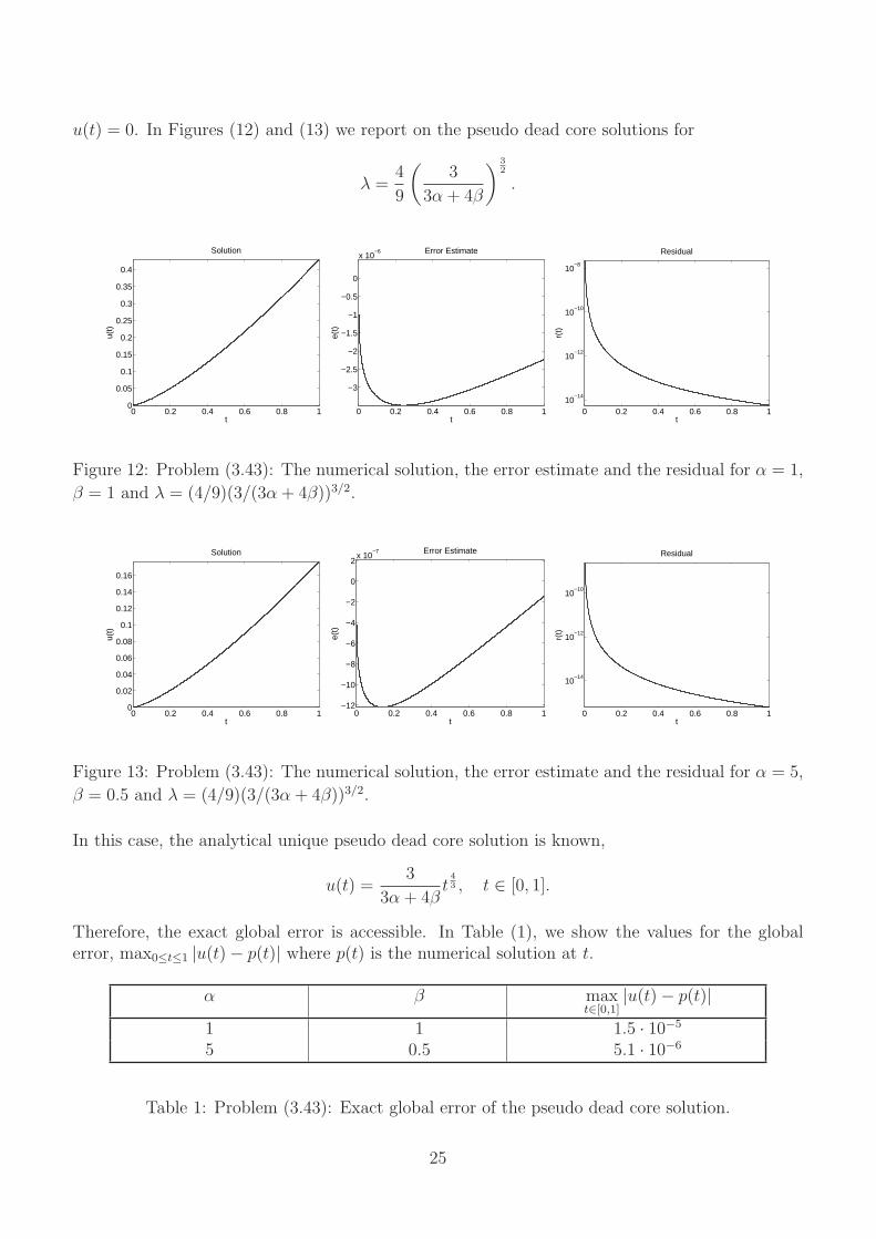
u(t) = 0. In Figures (12) and (13) we report on the pseudo dead core solutions for

λ =4

9

(

3

3α + 4β

) 3

2

.

0 0.2 0.4 0.6 0.8 10

0.05

0.1

0.15

0.2

0.25

0.3

0.35

0.4

t

u(t)

Solution

0 0.2 0.4 0.6 0.8 1

−3

−2.5

−2

−1.5

−1

−0.5

0

x 10−6

t

e(t)

Error Estimate

0 0.2 0.4 0.6 0.8 110

−14

10−12

10−10

10−8

t

r(t)

Residual


β = 1 and λ = (4/9)(3/(3α + 4β))3/2.

0 0.2 0.4 0.6 0.8 10

0.02

0.04

0.06

0.08

0.1

0.12

0.14

0.16

t

u(t)

Solution

0 0.2 0.4 0.6 0.8 1−12

−10

−8

−6

−4

−2

0

2x 10

−7

t

e(t)

Error Estimate

0 0.2 0.4 0.6 0.8 1

10−14

10−12

10−10

t

r(t)

Residual


β = 0.5 and λ = (4/9)(3/(3α + 4β))3/2.

In this case, the analytical unique pseudo dead core solution is known,

u(t) =3

3α + 4βt

4

3 , t ∈ [0, 1].

Therefore, the exact global error is accessible. In Table (1), we show the values for the globalerror, max0≤t≤1 |u(t) − p(t)| where p(t) is the numerical solution at t.

α β maxt∈[0,1]

|u(t) − p(t)|1 1 1.5 · 10−5

5 0.5 5.1 · 10−6

Table 1: Problem (3.43): Exact global error of the pseudo dead core solution.

25

3.3 Dead Core Solutions

We now deal with the dead core solutions of the problem. Note that they only occur for

λ >4

9

(

3

3α + 4β

) 3

2

.

Moreover, the relation between λ and t1, where t1 is such that the solution vanishes on [0, t1], isgiven by

λ =4

9√

1 − t1

(

3

3α(1 − t1) + 4β

) 3

2

.

Also, the dead core solution is known,

u(t) =

(

3

2

√λ(t − t1)

) 4

3

, t ∈ [t1, 1].

For the experiments, we used t1 = 0.2 and t1 = 0.8, in order to solve the problem,

u′′(t)√

u(t)u(t) = λu(t), t ∈ [t1, 1], (3.44a)

u′(t1) = 0, αu(1) + βu′(1) = 1, α > 0, β > 0. (3.44b)

Clearly, if we approached the problem (3.44) directly, we had to use the knowledge of t1 which isnot available in general. Therefore, it is especially important to note that we were able to find thedead core solution without explicit knowledge of t1 by treating the problem (3.43), formulated onthe whole interval [0, 1],

u′′(t)√

u(t)u(t) = λu(t), t ∈ [0, 1],

u′(0) = 0, αu(1) + βu′(1) = 1, α > 0, β > 0,

instead of solving (3.44).In Figures 14 and 15 we report on the numerical test runs for α = 1, β = 1, and two values of t1,t1 = 0.2 and t1 = 0.8, respectively.

26

0 0.2 0.4 0.6 0.8 10

0.05

0.1

0.15

0.2

t

u 0(t)

Initial profile

0 0.2 0.4 0.6 0.8 10

0.05

0.1

0.15

0.2

0.25

0.3

0.35

t

u(t)

Solution

0 0.2 0.4 0.6 0.8 1

−15

−10

−5

0

x 10−6

t

e(t)

Error Estimate

0 0.2 0.4 0.6 0.8 1

10−60

10−40

10−20

t

r(t)

Residual

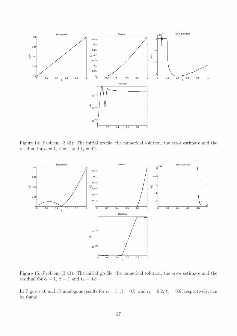
Figure 14: Problem (3.43): The initial profile, the numerical solution, the error estimate and theresidual for α = 1, β = 1 and t1 = 0.2.

0 0.2 0.4 0.6 0.8 10

0.05

0.1

0.15

0.2

t

u 0(t)

Initial profile

0 0.2 0.4 0.6 0.8 10

0.02

0.04

0.06

0.08

0.1

0.12

t

u(t)

Solution

0 0.2 0.4 0.6 0.8 1

−2

−1.5

−1

−0.5

0x 10

−5

t

e(t)

Error Estimate

0 0.2 0.4 0.6 0.8 1

10−200

10−100

t

r(t)

Residual

Figure 15: Problem (3.43): The initial profile, the numerical solution, the error estimate and theresidual for α = 1, β = 1 and t1 = 0.8.

In Figures 16 and 17 analogous results for α = 5, β = 0.5, and t1 = 0.2, t1 = 0.8, respectively, canbe found.

27

0 0.2 0.4 0.6 0.8 10

0.1

0.2

0.3

0.4

0.5

0.6

0.7

0.8

t

u 0(t)

Initial profile

0 0.2 0.4 0.6 0.8 10

0.02

0.04

0.06

0.08

0.1

0.12

0.14

0.16

t

u(t)

Solution

0 0.2 0.4 0.6 0.8 1

−4

−3

−2

−1

0

x 10−6

t

e(t)

Error Estimate

0 0.2 0.4 0.6 0.8 1

10−80

10−60

10−40

10−20

t

r(t)

Residual

Figure 16: Problem (3.43): The initial profile, the numerical solution, the error estimate and theresidual for α = 5, β = 0.5 and t1 = 0.2.

0 0.2 0.4 0.6 0.8 10

0.05

0.1

0.15

0.2

t

u 0(t)

Initial profile

0 0.2 0.4 0.6 0.8 10

0.02

0.04

0.06

0.08

0.1

0.12

t

u(t)

Solution

0 0.2 0.4 0.6 0.8 1

−16

−14

−12

−10

−8

−6

−4

−2

0x 10

−6

t

e(t)

Error Estimate

0 0.2 0.4 0.6 0.8 1

10−300

10−200

10−100

r(t)

Residual

Figure 17: Problem (3.43): The initial profile, the numerical solution, the error estimate and theresidual for α = 5, β = 0.5 and t1 = 0.8.

Table 2 contains the information on the exact global error of the numerical dead core solution.We report on its maximal value maxt∈[0,1] |u(t)− p(t)| for a wide range of parameters. Obviously,dead core solutions can be found without exact use of the known solution structure, but the initial

28

profile must be chosen carefully to guarantee the Newton iteration to convergence.

α β t1 maxt∈[0,1]

|u(t) − p(t)|1 1 0.2 9.7 10−4

1 1 0.5 1.2 10−3

1 1 0.8 1.7 10−3

0.5 1.5 0.2 1.5 10−3

0.5 1.5 0.5 1.5 10−3

0.5 1.5 0.8 1.2 10−3

0.5 0.8 0.3 5.5 10−2

0.5 0.8 0.5 1.8 10−3

0.5 0.8 0.8 2.8 10−3

0.3 5 0.2 7.4 10−4

0.3 5 0.5 7.1 10−4

0.3 5 0.8 6.2 10−4

5 0.5 0.2 3.6 10−4

5 0.5 0.5 6.2 10−4

5 0.5 0.8 6.7 10−4

Table 2: Maximum of the exact global error of the numerical dead core solution.

3.4 Positive Solutions of Problem (1.3)

In this section we deal with problem (1.3). Since this problem is very involved, we decided tosimulate it numerically first in order to provide some preliminary information about its solution.The numerical treatment of (1.3) turned out to be not at all straightforward, but nevertheless, fora certain choice of parameters, γ = 3, ρ = 2, ν = 2, and α = 0.1, β = 1, we were able to solve theproblem and provide the error estimate and the residual for its approximative solution. We haveapplied the pathfollowing strategy implemented in bvpsuite to the boundary value problem

((u′(t))3)′ +u′(t)

t2= ϑ

(

1√

u(t)+ (u′(t))2

)

, 0 < t ≤ 1, (3.45a)

u′(0) = 0, 0.1u(1) + u′(1) = 1, ϑ = λ. (3.45b)

29

0.6 0.8 1 1.2 1.4 1.6 1.8

1

2

3

4

5

6

7

8

λ

||p||

Figure 18: Graph of the ‖p‖ − λ path obtained in 76 steps of the pathfollowing procedure, where‖p‖ = max

t∈[0,1]|p(t)|. The turning point has been found at λ ≈ 1.8442.

In Figures 19 to 28, we present numerical results for problem (3.45). The values of λ for whichwe were able to calculate the associated numerical solutions, are shown in Figure 18. Accordingto Figure 18, we have found a turning point at λ ≈ 1.8442. In a certain region below this value,there exist for any λ two different positive solutions.In order to start the pathfollowing procedure we set λ = 0.5 and used u ≡ 1 as an initial profile.For each further step, we used the solution from the previous step as an initial profile. The solutioncorresponding to the values of λ shown in Figures 19 and 20 is unique.

0 0.2 0.4 0.6 0.8 1

7.63

7.64

7.65

7.66

7.67

7.68

7.69

7.7

t

u(t)

Solution

0 0.2 0.4 0.6 0.8 1

−2.4

−2.35

−2.3

−2.25

−2.2

x 10−13

t

e(t)

Error Estimate

0 0.2 0.4 0.6 0.8 1

10−15

10−14

10−13

t

r(t)

Residual

Figure 19: Problem (3.45): The numerical solution, the error estimate and the residual for λ =0.69901190254861.

30

0 0.2 0.4 0.6 0.8 16.26

6.28

6.3

6.32

6.34

6.36

6.38

t

u(t)

Solution

0 0.2 0.4 0.6 0.8 1

−1

−0.5

0

0.5

1

1.5

x 10−14

t

e(t)

Error Estimate

0 0.2 0.4 0.6 0.8 1

10−15

10−14

10−13

10−12

t

r(t)

Residual


For λ ≈ 1.215 we have found two different positive solutions, cf. Figures 21 and 22.

0 0.2 0.4 0.6 0.8 1

5.76

5.78

5.8

5.82

5.84

5.86

5.88

t

u(t)

Solution

0 0.2 0.4 0.6 0.8 10

0.2

0.4

0.6

0.8

1

1.2

1.4x 10

−14

t

e(t)

Error Estimate

0 0.2 0.4 0.6 0.8 110

−15

10−14

10−13

10−12

t

r(t)

Residual


0 0.2 0.4 0.6 0.8 1

0.1

0.2

0.3

0.4

0.5

t

u(t)

Solution

0 0.2 0.4 0.6 0.8 10

1

2

3

4

5

6x 10

−14

t

e(t)

Error Estimate

0 0.2 0.4 0.6 0.8 1

10−14

10−12

10−10

t

r(t)

Residual


Also, for λ ≈ 1.425, two different positive solutions exist, see Figures 23 and 24.

31

0 0.2 0.4 0.6 0.8 1

4.9

4.92

4.94

4.96

4.98

5

5.02

5.04

5.06

t

u(t)

Solution

0 0.2 0.4 0.6 0.8 1

−1

−0.5

0

0.5

1

1.5

x 10−14

t

e(t)

Error Estimate

0 0.2 0.4 0.6 0.8 1

10−15

10−14

10−13

10−12

t

r(t)

Residual


0 0.2 0.4 0.6 0.8 10.3

0.35

0.4

0.45

0.5

0.55

0.6

0.65

0.7

t

u(t)

Solution

0 0.2 0.4 0.6 0.8 10.8

1

1.2

1.4

1.6

1.8

x 10−13

t

e(t)

Error Estimate

0 0.2 0.4 0.6 0.8 1

10−14

10−12

10−10

t

r(t)

Residual


Interestingly, solutions found in the vicinity of the turning point change rather fast, although thevalues of λ do not, see Figures 25 to 27.

0 0.2 0.4 0.6 0.8 1

2.15

2.2

2.25

2.3

2.35

2.4

t

u(t)

Solution

0 0.2 0.4 0.6 0.8 1

1.32

1.34

1.36

1.38

1.4

1.42

1.44

1.46

1.48x 10

−12

t

e(t)

Error Estimate

0 0.2 0.4 0.6 0.8 1

10−14

10−12

t

r(t)

Residual


32

0 0.2 0.4 0.6 0.8 1

2

2.05

2.1

2.15

2.2

2.25

t

u(t)

Solution

0 0.2 0.4 0.6 0.8 1

1

2

3

4

5

6

7

8

9

x 10−14

t

e(t)

Error Estimate

0 0.2 0.4 0.6 0.8 1

10−14

10−13

10−12

10−11

t

r(t)

Residual


0 0.2 0.4 0.6 0.8 1

1.8

1.85

1.9

1.95

2

2.05

2.1

t

u(t)

Solution

0 0.2 0.4 0.6 0.8 1

4.2

4.4

4.6

4.8

5

x 10−13

t

e(t)

Error Estimate

0 0.2 0.4 0.6 0.8 1

10−14

10−13

10−12

10−11

t

r(t)

Residual


Finally, in the last step of the procedure, we obtained a solution which nearly reaches a pseudodead core solution with p(0) ≈ u(0) ≈ 0.

0 0.2 0.4 0.6 0.8 1

0.1

0.2

0.3

0.4

0.5

t

u(t)

Solution

0 0.2 0.4 0.6 0.8 10

1

2

3

4

5

6x 10

−14

t

e(t)

Error Estimate

0 0.2 0.4 0.6 0.8 1

10−14

10−12

10−10

10−8

t

r(t)

Residual


33

References

[1] R. P. Agarwal, D. O’Regan and S. Stanek. Dead core problems for singular equationswith φ-Laplacian, Bound. Value Probl. Vol. 2007, Article ID 18961.

[2] R. P. Agarwal, D. O’Regan and S. Stanek. Positive and dead core solutions problemsof singular Dirichlet boundary value problems with φ-Laplacian, Comput. Math. Appl. 54(2007), 255–266.

[3] R. P. Agarwal, D. O’Regan and S. Stanek. Dead cores of singular Dirichlet boundaryvalue problems with φ-Laplacian, Appl. Math., accepted for publication.

[4] R. Aris. The mathematical theory of diffusion and reaction in permeable catalysts, Claren-don Press, Oxford, 1975.

[5] U. Ascher, R. M. M. Mattheij, and R. D. Russell. Numerical solution of boundaryvalue problems for ordinary differential equations, Prentice-Hall, Englewood Cliffs, New York,1988.

[6] W. Auzinger, O. Koch, and E. Weinmuller. Efficient collocation schemes for singularboundary value problems, Numer. Algorithms 31 (2002), 5–25.

[7] W. Auzinger, G. Kneisl, O. Koch, and E. Weinmuller. A collocation code forboundary value problems in ordinary differential equations, Numer. Algorithms 33 (2003),27–39.

[8] W. Auzinger, O. Koch, and E. Weinmuller. Efficient mesh selection for collocationmethods applied to singular BVPs, J. Comput. Appl. Math. 180 (2005), 213–227.

[9] J. V. Baxley and G. S. Gersdorff. Singular reaction-diffusion boundary value problems,J. Differential Equations 115 (1995), 441–457.

[10] L. E. Bobisud. Asymptotic dead cores of reaction-diffusion equations, J. Math. Anal. Appl.147 (1990), 249–262.

[11] L. E. Bobisud. Behaviour of solutions for a Robin problem, J. Differential Equations 85(1990), 249–262.

[12] L. E. Bobisud, D. O’Regan and W. D. Royalty. Existence and nonexistence for asingular boundary value problem, Appl. Anal. 28 (1988), 245–256.

[13] C. J. Budd, O. Koch, and E. Weinmuller. Self-similar blow-up in nonlinear PDEs.AURORA TR-2004-15, Inst. for Anal. and Sci. Comput., Vienna Univ. of Technology, Austria,2004. Available at http://www.vcpc.univie.ac.at/aurora/publications/.

[14] C. J. Budd, O. Koch, and E. Weinmuller. Computation of Self-Similar Solution Profilesfor the Nonlinear Schrodinger Equation, Computing 77 (2006), 335–346.

[15] C. J. Budd, O. Koch, and E. Weinmuller. From Nonlinear PDEs to Singular ODEs,Appl. Numer. Math. 56 (2006), 413–422.

34

[16] G. Kitzhofer. Numerical treatment of implicit singular BVPs. Ph.D. Thesis, Inst. for Anal.and Sci. Comput., Vienna Univ. of Technology, Austria. In preparation.

[17] G. Kitzhofer, O. Koch, and E. Weinmuller. Collocation methods for the computationof bubble-type solutions of a singular boundary value problem in hydrodynamics. J. Sci.Comp. 32 (2007), 411–424.

[18] G. Kitzhofer, O. Koch, and E. Weinmuller. Pathfollowing for Essentially SingularBoundary Value Problems with Application to the Complex Ginzburg-Landau Equation.Accepted for BIT.

[19] I. Rachunkova, O. Koch, G. Pulverer, and E. Weinmuller. On a Singular Bound-ary Value Problem Arising in the Theory of Shallow Membrane Caps, Math. Anal. and Appl.332 (2007), 523–541.

[20] S. Stanek, G. Pulverer and E. Weinmuller. Analysis and numerical simulation ofpositive and dead core solutions of singular two-point boundary value problems, in press forComp. Math. Appl.

35

Analysis and numerical solutions of positive and dead core ...

Documents

Transcript of Analysis and numerical solutions of positive and dead core ...