Delft University of Technology

Analysis and modelling of performances of the HL (Hyperloop) transport system

van Goeverden, Kees; Milakis, Dimitris; Janic, Milan; Konings, Rob

DOI10.1186/s12544-018-0312-xPublication date2018Document VersionFinal published versionPublished inEuropean Transport Research Review

Citation (APA)van Goeverden, K., Milakis, D., Janic, M., & Konings, R. (2018). Analysis and modelling of performances ofthe HL (Hyperloop) transport system. European Transport Research Review, 10(2), [41].https://doi.org/10.1186/s12544-018-0312-x

Important noteTo cite this publication, please use the final published version (if applicable).Please check the document version above.

CopyrightOther than for strictly personal use, it is not permitted to download, forward or distribute the text or part of it, without the consentof the author(s) and/or copyright holder(s), unless the work is under an open content license such as Creative Commons.

Takedown policyPlease contact us and provide details if you believe this document breaches copyrights.We will remove access to the work immediately and investigate your claim.

This work is downloaded from Delft University of Technology.For technical reasons the number of authors shown on this cover page is limited to a maximum of 10.

ORIGINAL PAPER Open Access

Analysis and modelling of performances ofthe HL (Hyperloop) transport systemKees van Goeverden1* , Dimitris Milakis1, Milan Janic1 and Rob Konings2

Abstract

Introduction: Hyperloop (HL) is presented as an efficient alternative of HSR (High Speed Rail) and APT (Air PassengerTransport) systems for long-distance passenger transport. This paper explores the performances of HL and comparesthese performances to HSR and APT.

Methods: The following performances of the HL system are analytically modeled and compared to HSR and APT: (i)operational performance; (ii) financial performance; (iii) social/environmental performance.

Results: The main operational result is that the capacity of HL is low which implies a low utilization of the infrastructure.Because the infrastructure costs dominate the total costs, the costs per passenger km are high compared to those forHSR and APT. The HL performs very well regarding the social/environmental aspects because of low energy use, no GHGemissions and hardly any noise. The safety performance needs further consideration.

Conclusions: The HL system is promising for relieving the environmental pressure of long-distance travelling, but hasdisadvantages regarding the operational and financial performances.

Keywords: HL (Hyperloop) system, Performances, Long-distance transport, Modelling, Estimation

1 IntroductionThe competition between contemporary transport modeshas been rather constant over the past decades. However,this has not applied to the European long-distance passen-ger transport where the airlines have increased their marketshare substantively. Van Goeverden et al. [1] have estimatedthat air travel increased by about 45% between 2001 and2013 while usage of the alternative modes has been ratherstable (car, train) or declining (bus). The increasing domin-ance of air transport has enlarged the environmental im-pacts of long-distance transport and this trend is expectedto continue in the next decades [2, 3]. The aircraft highspeed in combination with comparatively low fares particu-larly those offered by low cost carriers has caused thatrequirements of travellers have become increasingly de-manding, thus leading to a pressure on modes to offer highservice quality particularly in terms of the shorter traveltimes, and low fares. In addition, the environmental impactof transport has gained increasing interest, implying a grow-ing concern with the further dominance of air transport

and a demand for more environmental-friendly competitivetransport alternatives. This is particularly the case since thecurrent transport modes have been trying to adapt theiroperational, commercial, environmental, and social perfor-mances, though being bounded by their technologies. Forthese technologies, marginal but not radical improvementshave been permanently made. Radical new technologies,which could offer significantly better performances, are stillrare and so far have not been able to enter the transportmarket successfully.The HL (Hyperloop) system is a new transport technol-

ogy in conceptual stage that is claimed to provide superiorperformances to HSR (High Speed Rail) and APT (AirPassenger Transport) system, particularly regarding thetravel time, transport costs, energy consumption, andtransport safety [4]. So far, studies on HL have focused onenabling technologies of the system such as the electro-magnetic levitation [5], the dynamics of the HL vehicleand the infrastructure [6–9], the implications of the HLfor bridge dynamics [10] and the impact of earthquakeforces on the HL vehicle [11]. Decker et al. [12] exploredthe feasibility of the HL system focusing on tradesbetween technical/design aspects and the associated cost.

* Correspondence: c.d.vangoeverden@tudelft.nl1Transport & Planning Department, Delft University of Technology, P.O.Box5048, 2600 GA Delft, the NetherlandsFull list of author information is available at the end of the article

European TransportResearch Review

© The Author(s). 2018 Open Access This article is distributed under the terms of the Creative Commons Attribution 4.0International License (http://creativecommons.org/licenses/by/4.0/), which permits unrestricted use, distribution, andreproduction in any medium, provided you give appropriate credit to the original author(s) and the source, provide a link tothe Creative Commons license, and indicate if changes were made.

van Goeverden et al. European Transport Research Review (2018) 10:41 https://doi.org/10.1186/s12544-018-0312-x

Finally, Janić [13, 14] analysed multiple performances (e.g.operational, economic, social, and environmental) of high-speed rail and compared them to competing modes, with-out including HL in his analysis though.Existing studies have not yet systematically explored the

HL system’s performances as compared to other transportmodes. This paper aims at filling in this gap in the literatureby exploring the operational, financial, and social/environ-mental performances of the HL system and comparingthem with those of the HSR and APT system. The resultsof such comparison are intended to underpin the discus-sion about the overall feasibility of the HL system.In addition to this introductory section, the paper

consists of four other sections. Section 2 provides a briefdescription of the considered HS (High Speed) transport sys-tems - already fully operational HSR and APT and still onthe conceptual stage HL system. Section 3 deals with ananalysis and analytical modelling of the above-mentionedperformances of the three systems. Section 4 gives a com-parison of the HL system’s performances with those of theHSR and APT. For such purpose, the inputs for estimatingindicators of performances of the latter two systems (HSRand APT) are extracted from the existing secondary sources(references). The final Section (5) summarizes the mainconclusions regarding the prospective advantages and disad-vantages of the HL system and provides some perspectiveson its market opportunities.

2 The HS (high speed) transport systemsIn this section, we present an overview of the deploy-ment and main technical characteristics of the threehigh speed transport systems considered in this study:HSR, ART and HL.

2.1 The HSR (high speed rail) systemThe HSR systems have been developing worldwide (Europe,Far East-Asia, and USA -United States of America-) as anactually innovative system within the railway transportmode, particularly as compared to its conventional passen-ger counterparts. The system has had different definitionsin the particular world’s regions. For example: In Japan, theHSR system is called ‘Shinkansen’ (i.e., ‘new trunk line’)whose trains can run at the speed of at least 200 km/hr.The system’s network has been built with the specifictechnical standards (i.e., dedicated tracks without the levelcrossings and the standardized and special loading gauge).In Europe the HSR system has included infrastructurespecially built and/or upgraded for the HS (High Speed)travel and considered to be a part of the Trans-Europeanrail transport system/network. Respecting the maximumspeed, the HSR lines have been categorized as Category I(for the speeds equal to or greater than 250 km/h), CategoryII (those specially upgraded for the speeds of about 200 km/h), and Category III (those upgraded with particular features

resulting from the topographical relief or the town-planningconstraints). In China, according to Order No. 34, 2013from the country’s Ministry of Railways, the HSR system hasbeen considered to be the new built passenger-dedicatedlines with (actual or reserved) speed equal to and/or greaterthan 250 km/h along these lines and 200 km/h along themixed (passenger and freight) lines. In the USA, the HSRsystem has mainly been considered as that providing the fre-quent express services between the major population centreson the distances from 200 to 600 mi (mile) with a few or nointermediate stops, at the speeds of at least 150 mph (mi/h)on the completely grade-separated, dedicated rights-of waylines (1 mi = 1.609 km) [14]. Table 1 gives an example ofdeveloping the HSR networks round the world.In addition, Fig. 1 shows the development of the pas-

senger transportation in the European HSR network.As can be seen, the volumes of transportation in terms of

p-km have continuously been growing over the specifiedperiod of time, which has been possible thanks to expand-ing the HSR network in particular European countries.

2.2 The APT (air passenger transport) systemThe APT has been permanently growing thanks toimproving the ‘aircraft capabilities’, the ‘airline strat-egy’ and ‘governmental regulation’ (Boeing, 1998). The‘aircraft capabilities’ has related to increasing speed,payload, and take-off-weight. Both the speed and pay-load have contributed to an enormous increase in theaircraft productivity, for more than 100 times duringthe last forty years. In particular, increase in the speedhas been noticeable over the last six decades as shownon Fig. 2.During the same period, the aircraft seat capacity has

increased from 21 to 32 at the aircraft DC3 to almost600 at Airbus A380. In addition, the ‘airline strategy’have permanently deployed bigger, faster, safer, and morefuel-efficient aircraft equipped with lower emission andless-noise engines. As well, the aircraft of various sizeshave been progressively engaged to efficiently matchmarkets in the different network configurations, routelength, and demand density. The ‘governmental regula-tion’ has mainly been leading towards liberalization ofthe national and partially international markets. That inUSA (1978) and EU (European Union) (1997) are someof the earliest cases. Consequently, the APT system has

Table 1 Development of the HSR network around the world [14]

Status Continent Total-world

Europe Asia Othersa)

In operation (km) 7351 15,241 362 22,954

Under construction (km) 2929 9625 200 12,754

Total (km) 10,280 24,866 562 35,708a)Latin America, USA, Africa

van Goeverden et al. European Transport Research Review (2018) 10:41 Page 2 of 17

been growing over time as shown by the exampleson Fig. 3.As can be seen, in both areas the volumes of air

passenger transportation have been generally growing inthe long term, with some fluctuations. As well, thevolumes of the world’s air passenger transportation havebeen growing at an annual rate of 4–6% up to about 7trillion p-km in the year 2015 [15].

2.3 The HL (Hyperloop) systemHistorically, several pneumatic and maglev trains similar toHL have been proposed at conceptual level primarily aimingto substantially reduce travel time compared to existingmodes, and therefore being adopted in the transport system.For example, in 1910 Robert Goddard designed a floatingtrain on magnets inside a vacuumed tunnel that could reach250 miles/hour covering the distance between Boston andNew York in 10 min. In 1972, RAND suggested that a veryhigh speed transit (VHST) system operating in undergroundevacuated tubes propelled by electromagnetic waves wouldbe technically feasible to travel coast-to-coast in the US inas low as 21 min [16]. Yet, this report recognized that polit-ical feasibility of such project would be very low.For the purpose of this analysis and modelling its perfor-

mances, the HL system is assumed to consist of five maincomponents: i) the line/tube including at least two paralleltubes and the stations along them, which enable oper-ations of the HL vehicles in both directions withoutinterfering with each other and embarking and disembarking

of passengers, respectively; ii) the fleet of HL vehicles, whichcan consist of a single and/or few coupled capsules (these areoperated by means of a magnetic linear accelerator posi-tioned at the stations, which would accelerate the vehicles/capsules with the support of rotors attached to each ofthem); iii) the vacuum pumps maintaining the vacuumconditions within the tubes and at the stations at the speci-fied parts; iv) the vehicle control system while operatingalong the line(s)/tube(s); and v) the maintenance systems forall previous components.The tubes will be based on elevated pillars except for tun-

nel sections, while the solar panels above the tubes willprovide the system with energy. The ultra-high vacuum ap-proximately at the level of 10− 8 Torr (British and Germanstandards; Torr = Toricheli) would be maintained in thetube (the atmospheric pressure is variable but standardisedat the level of 760 Torr or 1.013·105 Pa (Pascal)). Each sta-tion of the HL system is to be generally integrated withinthe tube. It would consist of three modules. The first one isthe chamber as a part of the vacuum tube handling thearriving HL vehicle (ultimately ‘arriving’ chamber). Afterthe vehicle enters, de-vacuuming of the chamber is carriedout, and the vehicle proceeds to the second module withthe normal atmospheric pressure where passengersembark and disembark the vehicle(s). After that, thevehicle(s) passes to the third chamber where at thatmoment normal atmospheric pressure prevails (ultimately‘departing’ chamber). Then it spends time until the cham-ber is de-vacuuming, leaves it, and proceeds along theline/tube. This vehicle handling process takes place ateach station of the line. The chambers are separated bythe hermetic doors enabling establishing and maintainingthe required air pressure in the above-mentioned order.The capsules would operate in the above-mentioned

low-pressure tube(s) on a 0.5–1.3 mm layer of air fea-turing the pressurized air and the aerodynamic lift asshown on Fig. 4. Under such conditions, they would beable to reach the maximum speed of vmax = 1.220 km/h[4]; the maximum inertial acceleration would be a+ =0.5 g; g = 9.81 m/s2.

Fig. 1 Development of the volumes of passenger transportation inthe European HSR network over time (Period: 1990–2015) [34]

Fig. 2 Development of the aircraft speed over time [35]

Fig. 3 Development of air passenger transport in EU 28 (EuropeanUnion) and USA (United States of America) over time [34]

van Goeverden et al. European Transport Research Review (2018) 10:41 Page 3 of 17

The vacuum pumps are installed to initially evacuateand later maintain the required level of vacuum inside thetubes and in the stations’ first and third chambers. Inparticular, creating vacuum within the tube implies aninitially large-scale evacuation of air and later on removalof the smaller molecules near the tubes’ walls using theheating techniques. These pumps would consume a rathersubstantive amount of energy. At the initial stage, theywould operate until achieving the above-mentioned requiredlevel of tube vacuum, then, be automatically stopped, andthe vacuum-lock isolation gates opened. In cases of air leak-age in some section(s), the corresponding gates will be closedand the pumps activated again. The pumps would be locatedalong the tube(s) in the required number depending on thevolumes of air to be evacuated, available time, and theirevacuation capacity. As far as de-vacuuming and vacuumingof chambers at the stations is concerned, the required num-ber of vacuum pumps will operate accordingly.Regarding the characteristics of operations within the

tube and at the station(s), the control of safe and efficientmovement of vehicles and maintaining the vacuum insidethe tube and at the station(s) would be provided by theconvenient traffic control and management system.Given the above-mentioned technical features, the HL

is envisioned to be a transport mode for the medium- tolong-distance travelling. As such, if operating along theroutes without substantive physical barriers, it seems to bea good alternative to APT. At present, the HL technologyis being tested in practice on the short test tracks withprototype (capsule) models.Musk [4] considers two variants of the HL system: ex-

clusively for passenger only and mixed for both passengerand freight. The latter has larger dimensions for both thetube and the capsules. For example, the diameter of thetube for the exclusive passenger variant is 2.23 m and forthe mixed passenger and freight variant is 3.3 m. The cap-sules for passengers only are of the standardized seatingcapacity of S = 28 seats/unit, the mixed passenger andfreight variant gives room for 14 passengers and 3 full sizeautomobiles per unit. In particular, those intended exclu-sively to passengers allow them only to sit since the lack

of space for walking through the vehicle(s). In addition,the capsules of both variants lack the toilets, which dimin-ishes the flexibility and applicability of the system becausethe vehicles would need to stop every 30–60 min for alonger time for toilet visits. The capsules of the passengerand freight variant seem to be sufficiently large to enablewalking through the vehicle and to visit a toilet when thisis built-in. Their frontal area is supposed to be 4.0 m2 andthe height about 1.9 m. The larger dimensions make thesystem more expensive, but they are essential for itsfunctionality for long-distance travelling. Therefore,our analysis regards the passenger+freight variant withthe larger dimensions. Unlike Musk [4], we assumethat it is fully utilized for passenger transport and thatthe seating capacity is equal to the capacity of thesmall dimensioned passenger only variant: 28 seats perunit. Room for the toilet can be gained by reducingthe luggage compartment. The larger dimensions ofthe vehicles imply that a larger volume for luggage isavailable per m2 area, and that the seating compart-ment has more room for storing luggage.

3 Modelling performances of the HL, HSR, andAPT systemThe development and adoption of transport innovationscan be influenced by multiple factors. According to [17]development and adoption of transport innovations is afunction of techno-economic, social and political feasi-bility. If any of those three minimum criteria is not metthen the transport innovation will not be adopted. Janic[13] suggests that the performance of a new transportsystem can be considered in different ways and from theperspectives of different stakeholders involved, i.e., theusers/customers, the transport operator, the governmen-tal authorities at different institutional levels, and thesociety. If the different interests of stakeholders are notsuccessfully balanced, they may block the implementa-tion of a new transport system. In this study, we explorethe operational, financial and social/environmental per-formances of HL that reflect its all feasibility dimensions

Fig. 4 Conceptual design and subsystems of the HL system (source: [4])

van Goeverden et al. European Transport Research Review (2018) 10:41 Page 4 of 17

(see Fig. 5). The performances of its counterparts HSRand APT are considered for the comparative purposes.

3.1 Operational performanceThe operational performance of the HL system generallyincludes the system capacity and the quality of services.The former is mainly relevant for the operators, and thelatter for the users/customers.

3.1.1 CapacitySimilarly to its counterparts, the HSR and APT, the HLsystem is characterized by its traffic and transport ‘ul-timate’ capacity. The ‘ultimate’ capacity is the capacity inthe case that everything functions perfectly. In practice,this condition is not met, and the ‘practical’ capacity willbe somewhat lower than the ‘ultimate’ capacity.

a) Traffic capacity

The traffic ‘ultimate’ capacity is defined by the max-imum number of vehicles, which can pass through the“reference location” for their counting in one directionduring a given period of time under conditions of con-stant demand for service. In case of the HL system, thisis actually the capacity of the infrastructure, i.e., sta-tions, segments between the stations, and the line/tubeas the whole.

i) Station(s)

The ‘ultimate’ capacity of the station (i) of a given HLline/tube can be ‘static’ and ‘dynamic’. The ‘static’ cap-acity can be defined by the number of tracks/places atthe station. The static capacity that is needed to handlethe vehicles of guided transport systems during the given

period (T) under conditions of constant demand for ser-vice can generally be estimated as follows:

ns=i ¼ μi−1 Tð Þ � τs=i ð1Þwhereμi-1(T) is the capacity on the (i-1) segment of the line/tube in terms of the maximum transport service fre-quency during the time period (T) (veh/min or h); andτs/i is the average time of occupying a track/place at astation (i) by the Hyperloop vehicle (min, h/track).In the case of the HL system the relation between

occupation time and capacity is more complex. Thevehicles pass through the three above mentioned cham-bers, an arriving chamber, a chamber for disembarkingand embarking passengers, and a departure chamber.The arriving and departure chambers function as locks.The static capacity is not related to the sum of these oc-cupation times by a vehicle of the three chambers (τs/i),because a) occupation times can overlap (e.g. vehicle 1can enter the arriving chamber while vehicle 2 is still oc-cupying the platform in chamber 2) –this enlarges thecapacity– and b) the arriving and departure chambersare for some time occupied while they are empty (adapt-ing the air pressure for the next vehicle) –this lowers thecapacity–. The static capacity of HL can be estimated as:

ns=i ¼ μi−1 Tð Þ � max τca=i; τp=i; τcd=i� � ð2Þ

whereτca/i is the average occupation time of the arriving cham-ber of station i for one vehicle (min)τp/i is the average occupation time of the platform of astation (i) by one vehicle (min).τcd/i is the average occupation time of the departingchamber of station i for one vehicle (min)

Fig. 5 The considered HL, HSR, and APT performances explored in this study

van Goeverden et al. European Transport Research Review (2018) 10:41 Page 5 of 17

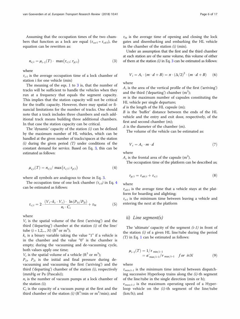
Assuming that the occupation times of the two cham-bers that function as a lock are equal (τca/i = τcd/i), theequation can be rewritten as:

ns=i ¼ μi−1 Tð Þ � max τc=i; τp=i� � ð3Þ

whereτc/i is the average occupation time of a lock chamber ofstation i for one vehicle (min)The meaning of the eqs. 1 to 3 is, that the number of

tracks will be sufficient to handle the vehicles when theyrun at a frequency that equals the segment capacity.This implies that the station capacity will not be criticalfor the traffic capacity. However, there may spatial or fi-nancial limitations for the number of tracks. One shouldnote that a track includes three chambers and each add-itional track means building three additional chambers.In that case the station capacity can be critical.The ‘dynamic’ capacity of the station (i) can be defined

by the maximum number of HL vehicles, which can behandled at the given number of tracks/spaces at the station(i) during the given period (T) under conditions of theconstant demand for service. Based on Eq. 3, this can beestimated as follows:

μs=i Tð Þ ¼ ns=i= max τc=i; τp=i� � ð4Þ

where all symbols are analogous to those in Eq. 3.The occupation time of one lock chamber (τc/i) in Eq. 4

can be estimated as follows:

τc=i ¼ 2 � V i−kc � Vcð Þ � ln P1i=P2ið Þni � Ci

þ τ0i ð5Þ

whereVi is the spatial volume of the first (‘arriving’) and thethird (‘departing’) chamber at the station (i) of the line/tube (i = 1,2,.., N) (ft3 or m3);kc is a binary variable taking the value “1” if a vehicle isin the chamber and the value “0” is the chamber isempty; during the vacuuming and de-vacuuming cycle,both values apply one time;Vc is the spatial volume of a vehicle (ft3 or m3);P1i, P2i is the initial and final pressure during de-vacuuming and vacuuming the first (‘arriving’) and thethird (‘departing’) chamber of the station (i), respectively(mmHg or Pa (Pascals));ni is the number of vacuum pumps at a lock chamber ofthe station (i);Ci is the capacity of a vacuum pump at the first and thethird chamber of the station (i) (ft3/min or m3/min); and

τ0i is the average time of opening and closing the lockgates and disembarking and embarking the HL vehiclein the chamber of the station (i) (min).Under an assumption that the first and the third chamber

at each station are of the same volume, this volume of eitherof them at the station (i) in Eq. 3 can be estimated as follows:

V i ¼ Ai � m � d þ Bð Þ ¼ π � Δ=2ð Þ2 � m � d þ Bð Þ ð6ÞwhereAi is the area of the vertical profile of the first (‘arriving’)and the third (‘departing’) chamber (m2);m is the maximum number of capsules constituting theHL vehicle per single departure;d is the length of the HL capsule (m);B is the ‘buffer’ distance between the ends of the HLvehicle and the entry and exit door, respectively, of thefirst and second chamber (m);Δ is the diameter of the chamber (m).The volume of the vehicle can be estimated as:

Vc ¼ Ac �m � d ð7ÞwhereAc is the frontal area of the capsule (m2).The occupation time of the platform can be described as;

τp=i ¼ τab=i þ τe=i ð8Þ

whereτab/i is the average time that a vehicle stays at the plat-form for boarding and alighting;τe/i is the minimum time between leaving a vehicle andentering the next at the platform

ii) Line segment(s)

The ‘ultimate’ capacity of the segment (i-1) in front ofthe station (i) of a given HL line/tube during the period(T) in Eq. 1 can be estimated as follows:

μi−1 Tð Þ ¼ 1=τ min=i−1¼ a−max=i−1=v max=i−1 f or i∈N ð9Þ

whereτmin/i-1 is the minimum time interval between dispatch-ing successive Hyperloop trains along the (i)-th segmentof the line/tube in the single direction (min or h);vmax/i-1 is the maximum operating speed of a Hyper-loop vehicle on the (i)-th segment of the line/tube(km/h); and

van Goeverden et al. European Transport Research Review (2018) 10:41 Page 6 of 17

a−max=i−1 is the maximum safe deceleration rate of the

Hyperloop vehicle on the (i)-th segment of the line/tube(m/s2).Equation 9 assumes that for safety reasons in each

pair of successive HL vehicle(s) moving in the samedirection the leading vehicle needs to be separated byat least the minimum breaking distance of the follow-ing vehicle.

iii) Line/tube

The line/tube capacity is the traffic capacity of the HLsystem and is defined as the lowest of the station andsegment capacities. From Eqs. 4 and 9, the ‘ultimate’capacity of a given HL line/tube in the single directioncan be estimated as follows:

μ Tð Þ ¼ min μs=i Tð Þ; μi−1 Tð Þh i

for i∈N ð10Þ

where all symbols are analogous to those in the previ-ous Eqs.Eq. 10 indicates that the ‘ultimate’ capacity of a given HL

line/tube is determined by the minimum ‘ultimate’ capacityof its (“critical”) segment(s) and/or the station(s). The‘ultimate’ capacity is higher than the ‘practical’ capacity. Thelatter can be described as:

μ Tð Þ� ¼ μ Tð Þ � Ui ð11Þwhere.μ(T)* is the practical traffic capacity;Ui is the utilisation rate of the ultimate traffic capacity

b) Transport capacity

The transport ‘ultimate’ capacity of a given HL line/tubecan be expressed by the maximum number of offeredseats in the single direction during the specified period oftime (T). Based on Eq. 10, it can be estimated as follows:

C Tð Þ ¼ μ Tð Þ �m � S ð12ÞwhereS is the number of seats per capsule (seats/capsule).The other symbols are analogous to those in Eqs. 6 and 10.The practical transport capacity can be described as:

C Tð Þ� ¼ μ Tð Þ� �m � S � θ ð13ÞwhereC(T)* is the practical transport capacity;

Θ is the average load factor of the vehicles (the ‘utilisa-tion rate’ of the ultimate vehicle capacity)For the practical applications, the actual transport

service frequency instead of the ‘ultimate’ transportcapacity of a HL line/tube in Eq. 10 needs to beconsidered. This frequency generally depends on thevolumes of demand, the HL vehicle’s average seatingcapacity per departure, and the average preferred loadfactor as follows:

f T ;Qð Þ ¼ min μ Tð Þ�; Q Tð Þm � s � θ

� �ð14Þ

whereQ(T) is the user/passenger demand during the period(T) in single direction (pass/h or pass/day);The other symbols are analogous to those in Eq. 13.The meaning of Eq. 14 is that if the frequency is set

equal to the practical traffic capacity (μ(T)*), the transportcapacity can be superfluous compared to the demand.That could be a reason to provide services with a lowerfrequency. In that case, the (scheduled) service frequencycan in some cases depend on a policy regarding a ‘de-cency’ transport service frequency.

c) Technical productivity

Multiplied by the average vehicle operating speedalong the line/tube the transport capacity gives an esti-mate of the technical productivity of a HL system undergiven conditions. From Eqs. 10 and 14, this maximumtechnical productivity is equal to:

TP Tð Þ ¼ min μ Tð Þ; f T ;Qð Þ½ � � v ð15Þwherev is the average speed of the HL vehicle(s) along theline/tube in the single direction (km/h).The other symbols are analogous to those in the previ-

ous Eqs.One can conclude from Eqs. 11 and 14 that f(T,Q)

never can exceed μ(T). Eq. 15 can then be rewritten as:

TP Tð Þ ¼ f T ;Qð Þ � v ð16ÞThe average speed ( v ) of the HL vehicle(s) in Eq. 16

can be estimated as follows:

v ¼ 2 � L=τ ð17Þwhere

L is the length of a given HL line/tube (km); andτ is the average turnaround time of the vehicles/capsules(min)The other symbols are analogous to those in previous

Eqs. (L ¼ PN−1i¼1 li).

van Goeverden et al. European Transport Research Review (2018) 10:41 Page 7 of 17

The technical productivity in Eq. 16 can also be esti-mated analogously.

d) Fleet size

Based on Eq. 3, the total time, which the HL vehicle(s)would spend at all stations along the line while movingin the same direction, is estimated as:

τs ¼ τs=1 þXN−1

i¼2

τs=i þ τs=N ð18Þ

whereN is the number of stations along the line/tube includingthe begin and end station (terminuses); andτs/1, τs/N is the average time, which the HL vehiclespends at the begin and the end station (terminus), re-spectively (min/veh).τs/i is the passing time of a vehicle through the station

(see also Eq. 1), This time is equal to:

τs=i ¼ 2 � τc=i þ τp=i ð19Þ

The other symbols are analogous to those in Eq. 3.The running time of the HL vehicle(s) along the line/

tube in the single direction is estimated as follows:

tL ¼XN−1

i¼1

12

v max=i

aþiþ liv max=i

þ 12

v max=i

a−i

� �ð20Þ

wherevmax/i is the maximum operating speed of the vehiclealong the (i)- the segment of the line (km/h); anda−i ; a

þi is the maximum safe deceleration and acceler-

ation rate, respectively, of the HL vehicle(s) on the (i)-the segment of the line (m/s2).The total turnaround time of the HL vehicle along the

line can be estimated based on Eqs. 18 and 20 as follows:

τ ¼ 2 � τs þ τLð Þ ð21Þ

Given the transport ‘ultimate’ capacity of a given line/tube (μ(T)) in Eq. 10 or the transport service frequencyin Eq. 14, and the average turnaround time per vehicle(τ) in Eq. 21, the required size of the HL fleet (Totalnumber of capsules) can be estimated as follows:

M Tð Þ ¼ min μ Tð Þ; f ðT ;QÞ½ � � τ �m ð22Þ

where all symbols are analogous to those in the previ-ous Eqs.

3.1.2 Quality of servicesThe quality of services influences (in addition to fares)the attractiveness of the HL system services and as suchindicates its relative advantage/disadvantage over thecompeting modes such as HSR and APT. The relative ad-vantage can be seen as the degree to which an innovationis perceived better than the product it replaces or com-petes with [18]. The relative advantage has considered tobe one of the strongest predictors of the outcome of thedecision on whether or not to adopt the innovation. Ingeneral, a new transport system does not need to performbetter on all aspects, but overall - taking all the relevantcharacteristics of the service into account - it should offersome added value, i.e., benefits to its users/passengers. Inthe given context, the attributes of quality service of theHL system such as a) door-to-door travel time; b) trans-port service frequency; and c) reliability of services areconsidered relevant for eventual mode/system choice.

a) Door-to-door travel time

The door-to-door travel time consists of the accessand egress time, schedule delay (including possibletime for luggage checking) at the boarding and alight-ing stations, in-vehicle time, and the interchange timebetween different HL vehicles and their particularservices at intermediate and end stations.

i) The access and egress time

The access and egress time depends on the interconnec-tivity between the HL system and the pre- and post-haulagesystems, the density of the HL stations, and the speed ofthe pre- and post-haulage systems (from the users’ doors tothe HL station, and vice versa). The access and egress timegenerally varies at particular HL stations depending on thelocal spatial and traffic conditions.

ii) The waiting time

The waiting time depends on the frequency of accessibleHL services. If there is no limitation on the accessibility,the waiting time is determined by the schedule delay.Based on Eq. 14, the schedule delay can be estimatedas follows:

SD Tð Þ ¼ 12� Tf T ;Qð Þ ð23Þ

where all symbols are as in the previous Eqs.In the case of full accessibility and frequent and

punctual services, the waiting time will be equal to theschedule delay. If the frequency is lower than 6/h, theaverage waiting time at the station will tend to be

van Goeverden et al. European Transport Research Review (2018) 10:41 Page 8 of 17

smaller than the schedule delay [19], but then there willbe some ‘hidden’ waiting time at the departure location. Ifseat reservation is obligatory, which is common for long-distance modes, the passengers can use only the servicefor which they reserved a seat; in that case, the frequencyof accessible services is just 1. Particularly in the case oflow frequencies, the timetables of connecting scheduledsystems as well as risk aversion of travellers for missingthe intended service can affect the waiting time.Low punctuality increases waiting time. The punctuality

of the HL system correlates with the homogeneity of succes-sive services (regarding to destination/routing, intermediatestops) and the scheduled buffer times. In the case of anetwork where some passengers also make interchanges,the policy on whether/how long to wait for the delayed con-necting services can additionally affect the punctuality andwaiting time.

iii) In-vehicle time and interchange time

The in-vehicle time of the HL system depends on thetravel distance, the average speed, and the stopping timeat the particular stations.If the HL system is set up as the network where some

travellers also make interchanges within it, the inter-change time will depend on the frequency of services,matching the timetables, punctuality, and the policy onwaiting for delayed connecting services.The in-vehicle time and the interchange time correlate

with the door-to-door distance. The access/egress andwaiting times are ‘fixed ‘times to this respect. The rela-tive values of the latter two time components will de-crease when the travel distances increase.

iv) Interchanges

The need to make interchanges generally diminishesthe overall quality of service because these may extendtravel times and make trips less convenient. In thelong-distance travel markets, which the HL system issupposed to penetrate, the users/passengers usually haveluggage with them. They generally will have to make atleast two interchanges (between the access mode andthe HL, and between the HL and the egress mode). Insome cases they have to make interchanges within the HLsystem. The opportunity of interchanges in the access andegress trips is related to the density of HL stations. Theopportunity of interchanges within the HL system isrelated to the design of the HL network.

b) Transport service frequency

The relevance of the service frequency as perceived bythe traveller will depend on the envisaged business plan

of HL: either as a ‘walk up’ service (i.e. direct accesswithout reservation in advance) or through an advancedobligatory seat reservation. In a scenario with the advancedseat reservation, on the one hand a lower frequency (i.e. 3–4dep/h) would be well acceptable, while on the other handthe offered service frequency at the time of booking will belower than the scheduled frequency in the case services arefully booked. In case of ‘walk up’ services the service fre-quency can also be lower than the scheduled frequency, i.e.when the demand exceeds temporally the offered capacity;then the imbalance between demand and supply will increasewaiting times [20].

c) Service reliability

The HL system has two major characteristics that enablea potential high reliability of its services. This is a com-pletely automated system, which as such, per definition,excludes delays due to the human errors. In addition, HLsystem operates in a closed environment which makes itresilient to the weather conditions. Of course, like any othertransport system, the reliability of the HL transport serviceswill depend on the technical reliability of all parts of thesystem (i.e., capsules, infrastructure, and control system).Table 2 gives the very preliminary estimates of the

above-mentioned indicators of operational performancesfor three considered systems - HL, HSR, and APT usingthe above-mentioned analytical models. Mode specificassumptions are presented below the table in the formof notes.As can be seen, based on the technical characteristics of

the HL, its transport service frequency is estimated to be12 dep/h, which is comparable to that of HSR. In addition,under given conditions, the HL system would perform bet-ter than its HSR and APT system counterpart only in termsof the indicator - the total station-station travel time.The station capacity depends on the choices of pump-

ing capacity and number of tracks. Based on Eq. 5, thepumping capacity for one lock chamber that makes thecapacity of the chamber equal to the segment capacitycan be calculated. Assuming one track, the required cap-acity can be described as:

ni � Ci ¼ 2 � V i−kc � Vcð Þ � ln P1i=P2ið Þτc=i � Ui−τ0i

¼ 2 � π � Δ=2ð Þ2 � m � d þ Bð Þ−kc � Ac �m � d� � � ln P1i=P2ið Þ60= f �Ui−τ0i

ð24Þ

Assuming that the chamber diameter is equal to thetube diameter (Δ = 3.3 m), and that m = 1, d = 30 m, B =3 m, kc = 0.5 (average of 0 and 1), Ac = 4.0 m2, P1i =0.74·1.013·105 Pa (Equivalent to the altitude of 2500 m

van Goeverden et al. European Transport Research Review (2018) 10:41 Page 9 of 17

MSL (Middle-Sea-Level)), P2i = 1·10–10 Pa (Ultra HighVacuum), f = 12/h, Ui = 0.8 and τ0i = 1 min, the requiredpumping capacity is about 5000 m3/min, e.g. 10 pumps(ni = 10) that produce 500 m3/min each (Ci = 500). Ifmore tracks are built, the calculated pumping capacityshould be divided by the number of tracks.

3.2 Financial performanceSimilarly as at the other transport modes and theirsystems, the financial performance of the HL system isdefined by its revenues, costs, and profits as the differ-ence between the former two. Consequently, the zeroprofitability achieved by the competitive prices giventhe costs could guarantee the bottom line for a stableeconomic viability of the HL system.

3.2.1 CostsThe costs consist of capital costs, operational costs, andoverhead costs. The capital costs are the costs for buildingthe infrastructure (tracks, stations), and the costs for pur-chasing the vehicles. The operational costs regard the cost

of maintenance of infrastructure and vehicles, and thecosts related to the operation of the vehicles and stations.The overhead costs comprise the capital and maintenancecost of real estate, and the staff costs.The estimation of the costs of a still not existing system

is a rather complex task. Therefore, in the given context,these costs are estimated based on published figures regard-ing the actual costs of the Maglev-system that are – to acertain extent – comparable to that of the HL system [21].The cost level is defined by the cost value, currency,

and time. One Euro in 2010 reflects a different cost levelthan either one US Dollar in 2010 or one Euro in 2015.For the sake of comparability, we will convert the figuresto Euros of 2015.

a) Capital cost for building tracks

The capital cost for building 1 km of line/tube is likelyto depend largely on the local conditions. Building in anempty area on flat sandy soil will be cheaper than build-ing in a highly urbanized area, in moorland, or in moun-tains. Crossing wide rivers or the need to build tunnelswill increase the costs. Musk [4] has estimated the costsof tubes on pylons and tubes in tunnels amounted€10.3 million/km and €34.0 million/km, respectively, forthe passenger + freight variant (converted into 2015€).For the purpose of comparison, there is the example

of a high-speed Maglev connection between ShanghaiPudong airport and the outskirts of the city in the formof a dual track of the length of 30 km and two stations(begin and end). Published costs are $1.2 billion and$1.33 billion [22, 23] (2002$US). A possible explanationfor the difference is the exclusion/inclusion of the twostations. Both amounts included the purchase cost ofthe vehicles. Excluding station costs and vehicle costs,the investment costs would have been about €41 millionper km track (€2015). Cost estimates for an extension ofthe line to Shanghai Hongqiao Airport were just thehalf: about €20 million €/km [24]. A reported reason forthe lower costs has been using all-concrete modulardesign that would reduce the cost by 30%. A secondpossible reason for the lower cost has been a more solidsoil. The current track has been built in an area withseismic activity and weak alluvial soil. This has requiredthe construction on piles, which raised the costs. An-other cost estimate of 34 million AU$/km (2008) or 26million €/km (2015) relates to the proposed Maglev linein the Melbourne area [25]. This estimate is somewhathigher than that for the Shanghai extension. Consideringthat the cost estimates generally are too low and there-fore the Melbourne estimate might be more realisticthan the Shanghai estimate, it is assumed that the costsof the Maglev track are in the order of 25 million €/kmunder favourable conditions.

Table 2 Some estimates of the indicators of operationalperformances of the HL system and its counterparts - HSR andAPT

Indicator HL HSRf) APTg)

Traffic capacity (veh/h)

- Segment 12a) –

- Station(s) p.m.b) –

- Linec) 12 12 –

Maximum service frequency (dep/h) 12d) 12 3

Vehicle capacity (seats/veh) 28 1000 130

Transport capacity (pax/h)e) 269e) 9600 312

Technical productivity (pax-km/h2)f) 327936f) 3360000g) 258968h)

Length of line (km) 600 600 600

Average operating speed (km/h) 965 264 407

In-vehicle time (minutes) 37.3 136.4 88.5

Schedule delay (min)i) 2.5 2.5 10

Total station-station travel time (min) 40.3 138.9 98.5a)At the maximum speed of: vmax = 1220 km/h and the maximum decelerationrate of: a- = 1.5m/s2 without stops along the line/tub, and a utilization rate ofthe infrastructure Ui = 80%b)The station capacity is so far undefined, because it depends on choicesregarding number of tracks and pumping capacity, and on the occupation timeof the platform by one vehicle. We assume for the latter 4 min, implying acapacity of no more than 15 veh./h in the case of one trackc)Min (Segment; station); Here we assume that the station capacity is not criticaland that the line capacity equals the segment capacityd)We assume that the demand volume is sufficient for providing the maximumfrequency, partly because the transport capacity of the Hyperloop is low at thehighest frequency, and partly because a quick scan for Europe revealed that thepotential demand for Hyperloop likely exceeds the capacity by far [32]e)At the maximum load factor θ: TC = f·θ·S; we assume for the Hyperloop θ = 80%f)At the maximum service frequency and speed, and load factor: TP = f·θ·S·vg)Average speed: v = 350 km/hh)Average speed: v = 830 km/hi)Based on Eq. 23

van Goeverden et al. European Transport Research Review (2018) 10:41 Page 10 of 17

The costs of 1 km of the HL line/tube will likely besomewhat higher than the cost of Maglev because thelatter system does not have the costs for tube con-struction and the costs for vacuum pumps. On theother hand, the HL does not need the concrete guide-way unlike the Maglev. Consequently, it is assumedthat the construction costs of the two systems aresimilar and therefore adopted to be 25 million €/kmfor the HL system built on solid soil This appearsmore than double the costs that were estimated byMusk [4] .Assuming that the actual cost of 40 million €/km for

the current Maglev track built on weak soil could havebeen reduced to about 35 million €/km by using amodular design, the latter figure is adopted for the HLsystem as well.The estimated costs for building tunnels at the HL system

of 34.0 million €/km [4] can only be compared with thecorresponding costs of the railway or road tunnels – theGotthard base tunnel consisting of two single-track tunnels:200 million €/km [26]; the Chuo Shinkansen railway linein Japan between Tokyo and Nagoya where 60% of theline goes through tunnels: 160 million €/km [27]; theChannel tunnel between France and Britain of the lengthof 50.5 km: 4.65 billion £/km (1990) or 190 million €/km(2015) [28]. These figures indicate that the tunnel costsfor a double track railway line are in the order of 200 mil-lion €/km. This is likely considerably higher than thecorresponding costs at the HL system. One of the mainreasons is a much smaller diameter of the HL tube – forexample, the two single-track Gotthard tunnels with di-ameters of about 9 m vs a HL tube of 3.3 m. The tunnelconstruction costs for two HL tubes might then evenbe somewhat lower than the costs for one single-trackrail tunnel. If it is assumed that the costs were underes-timated by about a factor 2, just like the argued under-estimation for the tube on pylons, the real costs for twoparallel tubes would be in the order of 70 million €/km.

b) Capital cost for building stations/terminals

The building costs for a station/terminal were esti-mated to be about 125 million $US (116 million €). Thecosts for the two stations of the current Maglev line nearShanghai could be 130 million US$ for two stations (i.e.,77 million €/station), which is significantly lower thanthe above-mentioned amount [4]. However, the HL sys-tem’s stations are more complex than that of the Maglevsystem because they should give access to vehicles in theevacuated tubes as mentioned above. Therefore, it is as-sumed that the cost per station of the HL system of€116 million is a fairly good estimate. Stations at nodesof the network where several lines inter-connect willlikely be more expensive.

c) Costs of vehicles

The costs for purchase of a vehicle (capsule) wereestimated to be about €1.42 million [4]. These are thecosts of a vehicle without toilets. Adding a toilet issupposed to increase the costs to about €1.52 million.For the purpose of comparison, the cost of one car-riage of a Maglev train with the capacity of 90 seatsare €12.5–15 million (compared to the capacity of theHL capsule of 28 seats) [25]. The average unit cost perseat which might be rather comparable are €0.14–0.17million for the Maglev and €0.054 million estimatedfor the HL. In the present case, it is assumed that theaverage unit cost for the HL capsule is 0.17 million €/seat,which is more than the threefold of the above-mentionedestimation by Musk [4]. The assumed cost of a capsule isthen €4.8 million.

d) The annual costs

The capital costs discussed above as incidental costscan be calculated as the annual costs (depreciation andinterest) as follows:

Cb eð Þ ¼Cb eð Þ−Re

Lt eð Þþ Cb eð Þ þ Re

2� It ð25Þ

whereCb(e) is the annual capital cost of the cost element e(€/track, station, and/or vehicle);CB(e) is the incidental capital cost of the cost element e (€);Re is the residual value of cost element e (€);Lt(e) is the life span of infrastructure element e (years); andIt is the interest rate (%/year).Table 3 gives an overview of the incidental investment

and the annual costs for the HL system. In all cases, it isassumed no residual value (Re= 0) for all cost elements,the interest rate: It = 4%/year, and the life spans as anaverage used in the EU-countries for the rail and roadinfrastructure and rolling stock [29].

Table 3 Investment and annual capital cost for the HL systeminfrastructure and vehicles

Cost element Investment cost(106 €/km or unit)a)

Annual cost(106 €/km or unit) a)

Life span(years)

Track infrastructure

- Pylons, solidsoil

25 0.92 60

- Pylons, weaksoil

35 1.28 60

- Tunnel 70 2.57 60

Station 116 4.64 50

Capsule 4.8 0.58 10a)The value 2015

van Goeverden et al. European Transport Research Review (2018) 10:41 Page 11 of 17

e) Maintenance costs of infrastructure and rolling stock

For the maintenance costs of the HL lines/tubes,stations, and rolling stock, a fixed ratio to the capitalcosts is assumed. The World Bank [30] states that thevariable component of rail infrastructure cost can varyfrom just a few percent to about 30% depending onthe intensity of use. The HL system is assumed to beheavily used, leading to relatively high maintenancecost, but the ratio to the capital cost will be smallerthan for rail because of the lack of physical contactbetween the vehicles and the infrastructure. Conse-quently, the ratio of 10% is assumed for both infra-structure and vehicles setting the annual maintenancecosts at 10% of the annual capital costs.

f ) Operating costs

The operating costs consist of the costs for staff in thevehicles and at the stations, and the traffic managementcosts. Generally the energy costs for moving the vehiclesare also part of the operating costs, but the HL is a spe-cial case because it is assumed to take energy from thesolar panels at the top of the tube. Some estimates indi-cate that such produced energy exceeds the energyconsumption by the vehicles [4]. The capital and main-tenance costs of the solar panels and the transmission ofenergy to the vehicles are then the only energy costs.The costs for employees in the vehicles and stations

depend on the organization, i.e., the number of employeesin the vehicles, and manpower needed for ticket sales andcontrol. In the present context, it is assumed that in eachcapsule one employee is present checking the seat belts,helping in the case of problems, and possibly providingsome food and drink. The staff at stations would includetwo employees per station controlling and possibly sellingtickets, and helping and guiding passengers. Assumingthat the average operation time of a capsule is 15 h/day,that stations are opened for 18 h/day, and that the average

working time of an employee is 7 h/day (including holidayand sickness absence), the number of full-time employeesfor a single capsule is 2.14 and for a station 5.14. Assum-ing an average annual wage of €35,000, the annual oper-ation cost for one capsule would be €75,000 and for astation €180,000. These costs appear to be relatively smallcompared to the capital cost.The traffic management costs depend on the inten-

sity of use and the complexity of the network. It isassumed that these costs are equal to the wage of oneemployee for each 1000 km of ‘double tube’. Assum-ing an operation time of 18 h per day, 2,57 fullemployees are needed per 1000 km of the line/tube.The relating annual costs would be €90,000/1000 km,or €90/km.

g) Overhead costs

The overhead costs include the capital and maintenancecost of real estate, and the staff costs. In the present con-text, it is assumed that the real estate costs are marginalcompared to the capital and maintenance costs of the HLinfrastructure. As such they are neglected. As far as thestaff costs, one overhead employee is assumed per eachten employees needed for operation, these costs are in-cluded by increasing the costs of operational staff for 10%.

h) Overview of the costs

Table 4 gives an overview of the annual unit costs ofthe HL system. At vehicles, the costs are also expressedper seat and seat-km, which makes them comparable tothat of other transport systems. For the calculation ofnumbers per seat km, we assume 28 seats per capsule,15 operating hours per day per capsule, and an averagedistance of 600 km per hour in the operating period.The vehicle cost per seat-km is very low compared to

the vehicle costs of other systems. Earlier calculations in-dicated that these costs ranged from 0.022–0,058 €/s-km

Table 4 Estimated annual costs of the HL system (€2015)

Cost element Unit Investment cost Maintenance cost Operating andoverhead cost

Total cost

Track infra

- Solid soil Km 917,000 91,700 100 1,010,000

- Weak soil Km 1,280,000 128,000 100 1,410,000

- Tunnel Km 2,570,000 257,000 100 2,820,000

Station Station 4,640,000 464,000 200,000 5,300,000

Capsule Vehicle 580,000 58,000 82,500 716,000

Seata) 21,000 2100 3000 26,000

Seat-kmb) 0.006 0.0006 0.0009 0.008a)Seat capacity: S = 28 seats/capsuleb)Seat capacity: S = 28 seats/capsule; Average speed in operating period: 600 km/h; Operating time: 15 h/day

van Goeverden et al. European Transport Research Review (2018) 10:41 Page 12 of 17

(1993€) at different public transport systems in theNetherlands [31]. These costs would be even higher whenexpressed in 2015€, but public transport provision hasbecome more cost-efficient since. An interesting findingin the study was that the costs are negatively correlated tothe speed of a system. The explanation is the fact thatmost cost components are time related, like the salary ofthe staff, which lowers the cost per km when the speedincreases. Very low costs for the extremely fast HL systemcould then be expected. An additional explanation is thatthe energy costs – the only cost component where theper-km cost increases with distance– are not included inthe HL vehicle costs.

3.2.2 Revenues/pricesAt an economically viable transport system as the HLsystem intends to be, the average unit price that theusers/passengers pay should at least cover the corre-sponding total average unit cost. These costs dependon the local conditions and the configuration of thesystem, including

� Soil condition, natural barriers; the impact isillustrated in Table 4.

� Average station spacing.� Connectivity; this defines together with the station

spacing the number of stations per km track that hasto be built; in the case of just one line connecting twostations, the number of stations per km at a givenstation spacing is about two times the number in alarge network.

� Frequency of the services; when the service frequencyincreases, the infrastructure costs are divided amongmore services and will be lower per ride.

� Load factor of the vehicles; this is inversely linearlycorrelated with the costs per passenger; because ofthe low transport capacity of the HL (see Table 2)and the high market potential because of the veryhigh speed (even higher than the airplane), generallya high load factor might be expected [32].

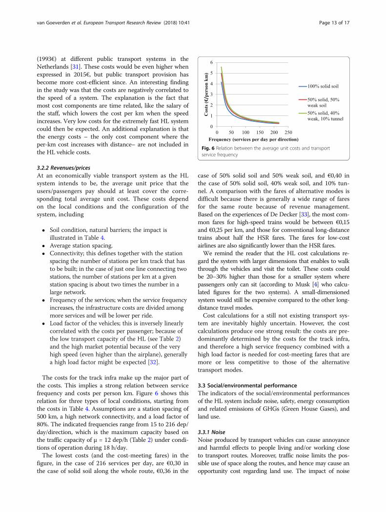
The costs for the track infra make up the major part ofthe costs. This implies a strong relation between servicefrequency and costs per person km. Figure 6 shows thisrelation for three types of local conditions, starting fromthe costs in Table 4. Assumptions are a station spacing of500 km, a high network connectivity, and a load factor of80%. The indicated frequencies range from 15 to 216 dep/day/direction, which is the maximum capacity based onthe traffic capacity of μ = 12 dep/h (Table 2) under condi-tions of operation during 18 h/day.The lowest costs (and the cost-meeting fares) in the

figure, in the case of 216 services per day, are €0,30 inthe case of solid soil along the whole route, €0,36 in the

case of 50% solid soil and 50% weak soil, and €0,40 inthe case of 50% solid soil, 40% weak soil, and 10% tun-nel. A comparison with the fares of alternative modes isdifficult because there is generally a wide range of faresfor the same route because of revenue management.Based on the experiences of De Decker [33], the most com-mon fares for high-speed trains would be between €0,15and €0,25 per km, and those for conventional long-distancetrains about half the HSR fares. The fares for low-costairlines are also significantly lower than the HSR fares.We remind the reader that the HL cost calculations re-

gard the system with larger dimensions that enables to walkthrough the vehicles and visit the toilet. These costs couldbe 20–30% higher than those for a smaller system wherepassengers only can sit (according to Musk [4] who calcu-lated figures for the two systems). A small-dimensionedsystem would still be expensive compared to the other long-distance travel modes.Cost calculations for a still not existing transport sys-

tem are inevitably highly uncertain. However, the costcalculations produce one strong result: the costs are pre-dominantly determined by the costs for the track infra,and therefore a high service frequency combined with ahigh load factor is needed for cost-meeting fares that aremore or less competitive to those of the alternativetransport modes.

3.3 Social/environmental performanceThe indicators of the social/environmental performancesof the HL system include noise, safety, energy consumptionand related emissions of GHGs (Green House Gases), andland use.

3.3.1 NoiseNoise produced by transport vehicles can cause annoyanceand harmful effects to people living and/or working closeto transport routes. Moreover, traffic noise limits the pos-sible use of space along the routes, and hence may cause anopportunity cost regarding land use. The impact of noise

Fig. 6 Relation between the average unit costs and transportservice frequency

van Goeverden et al. European Transport Research Review (2018) 10:41 Page 13 of 17

depends on the noise levels at sources, the number ofpeople exposed to them, and duration of the noise exposure.This implies that this performance at the considered systemsmainly depends on the routing of transport lines and speedand number of passing by vehicles.The HL is supposed to hardly produce any external

noise affecting relatively close population. This is due tothe fact that the HL is not in contact with the tube andtherefore there is no transfer of vibration. Any noisefrom the capsule itself will not be heard outside the tubeand the low air pressure inside the tube prevents noisefrom moving the capsule. The only potential source ofnoise could be the vacuum pumps, but these are assumedto produce negligible noise [21].

3.3.2 SafetyIn evaluating the performance of a transport system adistinction is usually made regarding the internal and ex-ternal safety. The internal safety relates to risk and damagecaused by incidents to the users/operator of the transportsystem itself. The external safety reflects the possible riskand damage of accidents/incidents to people and their liv-ing/working environment outside the systems. The HLsystem is a dedicated and closed transport system, exclud-ing any kind of interaction with other transport modesand its direct environment. Hence there are no externalsafety concerns, giving the HL system seemingly an ad-vantage over its prospective counterparts - APT and HSR.Internal safety benefits are expected because the HL sys-

tem is a completely automated system and hence excludesthe possibility of human errors. In addition the HL systemis supposed to be designed according to the fail-safe-principle: in case of danger (e.g., a rapid depressurizationin the capsule or tunnel), the “clever” systems will stop thecapsule and, if needed, will provide means of individualsalvation (e.g., oxygen masks for passengers). However,many safety issues still need further consideration, elabor-ation and testing, such as for example, evacuation ofpeople, stranded capsules, incorporation of emergencyexits, etc. [20].

3.3.3 Energy consumption and emissions of GHGs (greenhouse gases)The HL system is expected to be less energy demandingcompared to the HSR mainly due to having less frictionwith the track(s) and low air resistance due to the lowpressure in the tube. Some preliminary estimates havesuggested that the HL system can be about 2–3 timesmore energy-efficient than the HSR, and depending ontransport distances, about 3–6 times more energy-effi-cient than APT [20]. This is mainly because the HL sys-tem is intended to be completely propelled by theelectrical energy obtained by the solar panels on top ofthe tube(s). These are claimed to be able to generate

more than the energy needed to operate the system. Thisalso takes into account that sufficient energy can bestored (e.g., in the battery packs on board the vehicles)to operate the system at night, in periods of cloudy wea-ther, and in tunnels [4].In general, emissions of GHGs are directly related to the

energy consumption. If only emissions of GHGs by opera-tions are considered, regarding the above-mentionedprimary energy source, the HS system will not make anyof them. However, the indirect emissions from buildingthe infrastructure (lines and stations/terminals), rollingstock (capsules), and other equipment should be takeninto account in cases of dealing with the system’s life-cycleemissions of GHGs.

3.3.4 Land useIn general, land used to facilitate transport systems cannot,except for underground transportation, be used for otherpurposes, hence creating an opportunity cost. The valu-ation of land occupied by the HL system will be a functionof the space that is needed (width and length of the infra-structure) and the value of the land. The latter will dependheavily on the specific routing of the line. On the one hand,the HL system is planned to be elevated on pillars, so theeffective land occupation on the ground (net area of landneeded) can be limited. On the other hand, it remains to beseen if the space between the pillars can be used meaning-fully. Moreover, the elevated construction may bring alongvisual pollution. In general the total amount of land (grossarea of land) required for new transport infrastructure canbe minimized by maintaining the route as close as pos-sible to the existing transport infrastructure. The HLsystem’s tubes will be mounted side by side on elevatedpillars. For the small tubes – designed for passengertransport only – the size of the pillar that carries twotubes is about 3.5 m wide [21]. The tubes for mixedtraffic (passengers and freight) are larger and hence thepillars for these tubes are also expected to be larger, i.e.5.2 m. Since the pillars will be spaced averagely 30 mand the possibilities to use the space on the ground inbetween effectively is limited, the net area needed for1 km of HL system’s line will be about 0.5 ha. The aver-age gross area of taken land by the line is estimated tobe about 1.0 ha/km. Despite of more efficient land useof the HL system, it is likely that it will have higher costof land than, for instance, its HSR counterpart. This isbecause the HL system is less flexible than HSR systemin routing the line particularly in terms of accommo-dating to the sharp turns.

4 Overview of the indicators of performanceAn overview of the estimated indicators of perfor-mances of the HL, HSR, and APT systems accordingto the methodology presented in Sections 3.1 to 3.3 is

van Goeverden et al. European Transport Research Review (2018) 10:41 Page 14 of 17

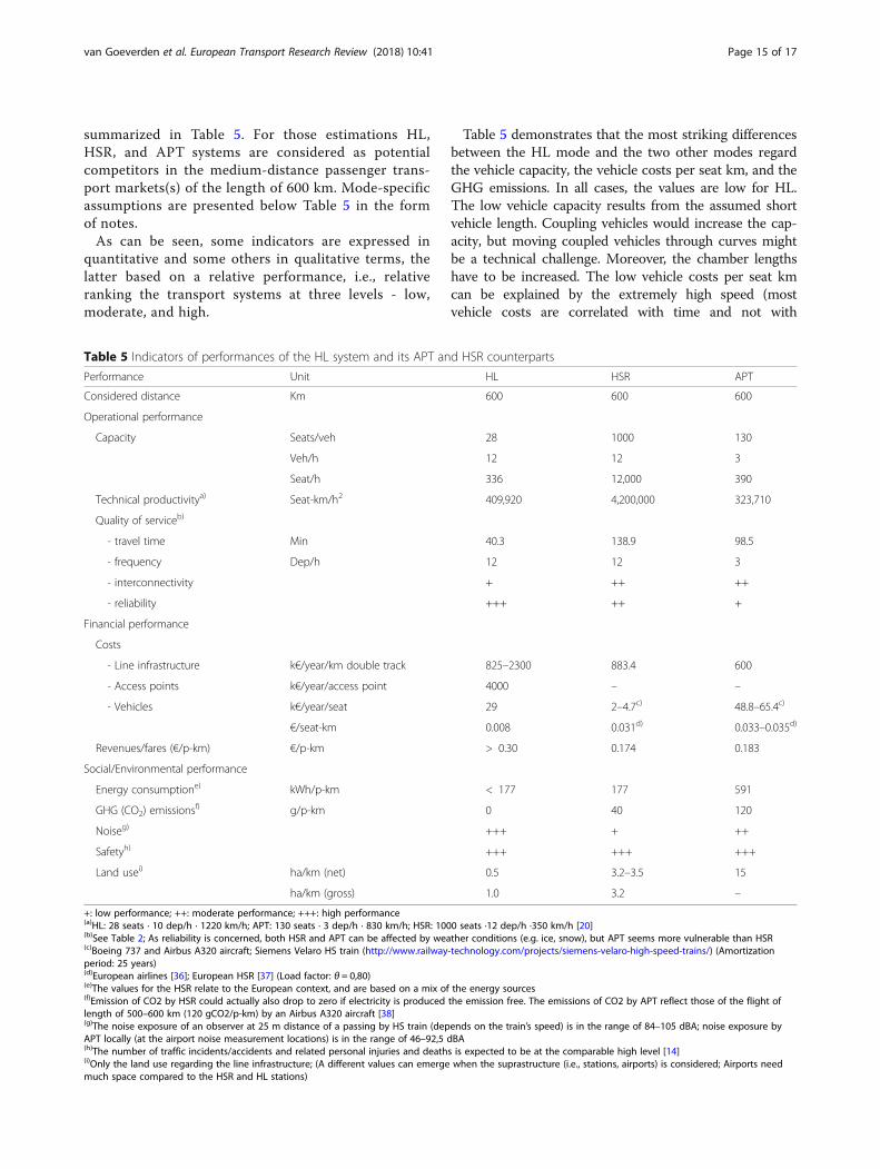
summarized in Table 5. For those estimations HL,HSR, and APT systems are considered as potentialcompetitors in the medium-distance passenger trans-port markets(s) of the length of 600 km. Mode-specificassumptions are presented below Table 5 in the formof notes.As can be seen, some indicators are expressed in

quantitative and some others in qualitative terms, thelatter based on a relative performance, i.e., relativeranking the transport systems at three levels - low,moderate, and high.

Table 5 demonstrates that the most striking differencesbetween the HL mode and the two other modes regardthe vehicle capacity, the vehicle costs per seat km, and theGHG emissions. In all cases, the values are low for HL.The low vehicle capacity results from the assumed shortvehicle length. Coupling vehicles would increase the cap-acity, but moving coupled vehicles through curves mightbe a technical challenge. Moreover, the chamber lengthshave to be increased. The low vehicle costs per seat kmcan be explained by the extremely high speed (mostvehicle costs are correlated with time and not with

Table 5 Indicators of performances of the HL system and its APT and HSR counterparts

Performance Unit HL HSR APT

Considered distance Km 600 600 600

Operational performance

Capacity Seats/veh 28 1000 130

Veh/h 12 12 3

Seat/h 336 12,000 390

Technical productivitya) Seat-km/h2 409,920 4,200,000 323,710

Quality of serviceb)

- travel time Min 40.3 138.9 98.5

- frequency Dep/h 12 12 3

- interconnectivity + ++ ++

- reliability +++ ++ +

Financial performance

Costs

- Line infrastructure k€/year/km double track 825–2300 883.4 600

- Access points k€/year/access point 4000 – –

- Vehicles k€/year/seat 29 2–4.7c) 48.8–65.4c)

€/seat-km 0.008 0.031d) 0.033–0.035d)

Revenues/fares (€/p-km) €/p-km > 0.30 0.174 0.183

Social/Environmental performance

Energy consumptione) kWh/p-km < 177 177 591

GHG (CO2) emissionsf) g/p-km 0 40 120

Noiseg) +++ + ++

Safetyh) +++ +++ +++

Land usei) ha/km (net) 0.5 3.2–3.5 15

ha/km (gross) 1.0 3.2 –

+: low performance; ++: moderate performance; +++: high performance(a)HL: 28 seats · 10 dep/h · 1220 km/h; APT: 130 seats · 3 dep/h · 830 km/h; HSR: 1000 seats ·12 dep/h ·350 km/h [20](b)See Table 2; As reliability is concerned, both HSR and APT can be affected by weather conditions (e.g. ice, snow), but APT seems more vulnerable than HSR(c)Boeing 737 and Airbus A320 aircraft; Siemens Velaro HS train (http://www.railway-technology.com/projects/siemens-velaro-high-speed-trains/) (Amortizationperiod: 25 years)(d)European airlines [36]; European HSR [37] (Load factor: θ = 0,80)(e)The values for the HSR relate to the European context, and are based on a mix of the energy sources(f)Emission of CO2 by HSR could actually also drop to zero if electricity is produced the emission free. The emissions of CO2 by APT reflect those of the flight oflength of 500–600 km (120 gCO2/p-km) by an Airbus A320 aircraft [38](g)The noise exposure of an observer at 25 m distance of a passing by HS train (depends on the train’s speed) is in the range of 84–105 dBA; noise exposure byAPT locally (at the airport noise measurement locations) is in the range of 46–92,5 dBA(h)The number of traffic incidents/accidents and related personal injuries and deaths is expected to be at the comparable high level [14](i)Only the land use regarding the line infrastructure; (A different values can emerge when the suprastructure (i.e., stations, airports) is considered; Airports needmuch space compared to the HSR and HL stations)

van Goeverden et al. European Transport Research Review (2018) 10:41 Page 15 of 17

distance) and the absence of energy costs: the costs for thesolar cells are part of the line infrastructure costs. TheGHG emissions are low (even zero) because it is assumedthat the solar cells provide all energy.

5 ConclusionsHyperloop (HL) is a new mode of transport that claims tobe a competitive and sustainable alternative to thelong-distance rail transport (HSR (High Speed Rail)) andthe medium-distance APT (Air Passenger Transport) sys-tem (less than or equal to 1.500 km). Taking into accountthat the performance of the HL system can be consideredin different ways and from the perspectives of differentstakeholders (i.e., passengers, transport operators, govern-ment authorities, and society) the operational, financial,social/environmental performances of the HL system havebeen investigated and evaluated.In comparing the HL with the HSR and APT system,

it has been found that the HL system has relativelypositive social/environmental performances, particu-larly in terms of the energy consumption, emissions ofGHGs, and noise. The HL system can potentially be avery safe mode, but both HSR and APT have also a verygood safety track record.A major weak point of the HL system technology appears

to be its rather low transport capacity, mainly due to thelow seating capacity of individual vehicles/capsules, whichaffects both the operational and the financial performance.Consequently, the investment costs of HL infrastructuremake up a large part of the total costs per seat-kilometre,raising the latter to a higher level than those of its counter-parts – HSR and APT. Hence, the break-even fares wouldalso be higher, even if the load factor is relatively high. Thisfinding suggests that HL-application may be limited to thepremium passenger transport market, in which there is‘willingness to pay’ for the strongest feature of HL systemservice carried out at the very high average speed.So far, the HL technology is in its infancy and there are

still many uncertainties around the system that need furtherexploration. From operational perspective, an important re-search issue is if and how the HL system transport capacitycould be increased, for instance, by increasing the numberseats or coupling several capsules into a single vehicle(‘train’). And also to what extent such change in capacitycould influence other operational, financial and socio/envir-onmental performances of the system. An initial studyexplored the relationship of HL vehicle capacity to total en-ergy consumption and found the former being ratherinsensitive to the latter (Decker et al., 2017). From financialperspective, further research is needed to more accuratelyestimate costs associated with HL development especiallywith respect to infrastructure (i.e. tracks, stations and vehi-cles) which form the larger part of the total costs perseat-kilometre. Apparently, further specification of these

costs requires more research on technological aspects ofthe system. Finally, from social/environmental perspective,further research is required in exploring the total life-cycleenergy consumption and GHGs emissions of the systemincluding infrastructure development (lines and stations/terminals), rolling stock (capsules), and operation of sub-systems such as the vacuum pumps. Moreover, estimationof social performance of the system would be improved byfurther research on possible implications of HL for socialwelfare such as accessibility to life-enhancing opportunitiesand creation of jobs (direct and indirect).

AcknowledgementsA previous version of this paper was presented at the BIVEC/GIBET TransportResearch Days 2017 in Liege, Belgium.

Authors’ contributionsDM conceived the research concept and wrote the theoretical and historicalbackground to the subject and the directions for future research. DM, MJ,KVG and RK designed the study. MJ described the HSR and APT systems andanalysed the operational performance of HL. KVG analysed the financialperformance of HL and contributed to the analysis of HL capacity. RKanalysed the social and environmental performance of HL. All authors readand approved the final manuscript.

Competing interestsThe authors declare that they have no competing interests.

Publisher’s NoteSpringer Nature remains neutral with regard to jurisdictional claims in publishedmaps and institutional affiliations.

Author details1Transport & Planning Department, Delft University of Technology, P.O.Box5048, 2600 GA Delft, the Netherlands. 2OTB, Research for the BuiltEnvironment, Delft University of Technology, Julianalaan 134, 2628 BL Delft,the Netherlands.

Received: 15 December 2017 Accepted: 22 August 2018

References1. Van Goeverden CD, Van Arem B, Van Nes R (2016) Volume and GHG

emissions of long-distance travelling by western Europeans. Transp Res D45:28–47. https://doi.org/10.1016/j.trd.2015.08.009

2. Lee DS, Fahey DW, Forster PM, Newton PJ, Wit RCN, Lim LL, Owen B,Sausen R (2009) Aviation and global climate change in the 21st century.Atmos Environ 43:3520–3537. https://doi.org/10.1016/j.atmosenv.2009.04.024

3. European Commission (2014) EU Energy, Transport and GHG Emissions,Trends to 2050, Reference Scenario 2013. Publications Office of theEuropean Union, Luxembourg

4. Musk E (2013) Hyperloop Alpha. SpaceX, Texas http://www.spacex.com/sites/spacex/files/hyperloop_alpha-20130812.pdf

5. Abdelrahman AS, Sayeed J, Youssef MZ (2018) Hyperloop transportationsystem: analysis, design, control, and implementation. IEEE Trans IndElectron 65(9):7427–7436. https://doi.org/10.1109/TIE.2017.2777412

6. Braun, J, Sousa, J, Pekardan, C (2017) Aerodynamic design and analysis ofthe hyperloop. AIAA Journal 55(12):4053-60 https://doi.org/10.2514/1.J055634

7. Chin, JC, Gray, JS, Jones, SM, Berton, JJ (2015) Open-source conceptualsizing models for the hyperloop passenger pod. 56th AIAA/ASCE/AHS/ASCStructures, Structural dynamics, and materials Conference, Kissimmee,Florida. https://doi.org/10.2514/6.2015-1587

8. Janzen R (2017) TransPod ultra-high-speed tube transportation: dynamics ofvehicles and infrastructure. Procedia Engineering 199:8–17 https://doi.org/10.1016/j.proeng.2017.09.142

van Goeverden et al. European Transport Research Review (2018) 10:41 Page 16 of 17

9. Yang Y, Wang H, Benedict M, Coleman D (2017) Aerodynamic Simulation ofHigh-Spee Capsule in the Hyperloop System. In: 35th AIAA AppliedAerodynamics Conference. American Institute of Aeronautics andAstronautics, Reston

10. Alexander NA, Kashani MM (2018) Exploring bridge dynamics for ultra-high-speed, Hyperloop, trains. Structures 14:69–74 https://doi.org/10.1016/j.istruc.2018.02.006

11. Heaton TH (2017) Inertial forces from earthquakes on a Hyperloop pod. BullSeismol Soc Am 107(5):2521–2524 https://doi.org/10.1785/0120170054

12. Decker K, Chin J, Peng A, Summers C, Nguyen G, Oberlander A, SakibG, Sharifrazi N, Heath C, Gray JS, Falck RD (2017) Conceptual Sizingand Feasibility Study for a Magnetic Plane Concept. In: 55th AIAAAerospace Sciences Meeting. American Institute of Aeronautics andAstronautics, Reston

13. Janić M (2003) Multicriteria evaluation of high-speed rail, Transrapid maglevand air passenger transport in Europe. Transp Plan Technol 26(6):491–512https://doi.org/10.1080/0308106032000167373

14. Janić M (2016) A multidimensional examination of performances of HSR(high-speed rail) systems. Journal of Modern Transportation 24(1):1–21https://doi.org/10.1007/s40534-015-0094-y

15. AIRBUS (2017) Growing Horizons 2017/2036: Global Market Forecast.AIRBUS, S.A.S, Blagnac Cedex, France

16. Salter RM (1972) The Very High Speed Transit System. RAND Corporation,Santa Monica

17. Feitelson E, Salomon I (2004) The political economy of transportinnovations. In: Beuthe M, Himanen V, Reggiani A, Zamparini L (eds)Transport development and innovations in an evolving world. Springer,Berlin, pp 11–26

18. Tidd J, Bessant J, Pavitt K (2001) Managing innovation, integrating technological,market, and organizational change. John Wiley and Sons, Chichester

19. Weber W (1966) Die Reisezeit der Fahrgäste öffentlicher Verkehrsmittel inAbhängigkeit von Bahnart und Raumlage. Forschungsarbeiten desVerkehrswissenschaftlichen Instituts an der Technischen HochschuleStuttgart, Stuttgart

20. Taylor CT, Hyde DJ, Barr LC (2016) Hyperloop commercial feasibility analysis:high level overview. Volpe (US Department of Transport), Cambridge

21. Wilkinson J (2016) A comparison of Hyperloop performances against highspeed rail and air passenger transport using multi-criteria analysis: casestudy of the San Francisco-Los Angeles corridor. Minor thesis, DelftUniversity of technology, Delft

22. Antlauf W, Bernardeau FG, Coates KC (2004) Fast track. Civil Engineering,The Magazine of the American Society of Civil Engineers 74(11):37–43

23. Wikipedia: https://en.wikipedia.org/wiki/Transrapid, assessed 31 October 201624. Wikipedia: https://en.wikipedia.org/wiki/Maglev, assessed 31 October 201625. TKTA: ThyssenKrupp Transrapid Australia (2008) ThyssenKrupp Transrapid

Australia submission in response to East West link needs assessment report“Investing in Transport”. ThyssenKrupp Transrapid Gmbh, Kassel

26. Wikipedia: https://en.wikipedia.org/wiki/Gotthard_Base Tunnel, assessed 31October 2016

27. Quora: https://www.quora.com/What-are-the-cost-differences-between-Maglev-and-conventional-high-speed-rail, assessed 31 October 2016

28. Wikipedia: https://en.wikipedia.org/wiki/Channel_Tunnel, assessed 31 October 201629. Ecorys transport, CE Delft (2005) Infrastructure expenditures and costs,

Practical guidelines to calculate total infrastructure costs for five modes oftransport, final report. Rotterdam. https://ec.europa.eu/transport/sites/transport/files/themes/infrastructure/studies/doc/2005_11_30_guidelines_infrastructure_report_en.pdf, assessed 31 October 2016

30. The World Bank (2011) Railway Reform: Toolkit for Improving Rail SectorPerformance. The World Bank, Washington

31. Goeverden V, CD Peeters PM (2006) Suspending subsidies for publictransport, its impacts on the public transport system in the Netherlands.85th annual meeting of the Transportation Research Board, Washington

32. Van Goeverden CD, Janić M, Milakis D (2018) Is Hyperloop helpful inrelieving the environmental burden of long-distance travel? An explorativeanalysis for Europe. Proceedings international conference on transport,climate change and clean air, Gif-sur-Yvette. https://www.iip.kit.edu/downloads/WCTR_SIGf2_2018_BookOfAbstracts.pdf, assessed 1 July 2018

33. De Decker K (2013) High Speed Trains are Killing the European RailwayNetwork. Low-tech Magazine 15, http://www.lowtechmagazine.com/2013/12/high-speed-trains-are-killing-the-european-railway-network.html.Assessed 31 Oct 2016.

34. EC (2017) EU Transport in Figures. Statistical Pocketbook 2017. EuropeanCommission. Publications Office of the European Union, Luxembourg, p 164

35. Janić M (2007) The sustainability of air transportation: quantitative analysisand assessment. Ashgate Publishing Company, Farnham

36. EEC (2015) Standard Inputs for EUROCONTROL Cost-Benefit Analyses.Edition Number: 7.0 Edition Date: November 2015. European Organisationfor the Safety of Air Navigation (EUROCONTROL), Brussels

37. UIC (2010) High speed rail: fast track to sustainability. International Union ofRailways, Paris, France, http://www.hsr.ca.gov/docs/about/business_plans/BPlan_2012LibraryCh7FastTrack.pdf. Accessed 1 Apr 2017.

38. ICAO (2016) Carbon Emissions Calculator, https://www.icao.int/environmental-protection/CarbonOffset/Pages/default.aspx. Accessed 1 Apr 2017.

van Goeverden et al. European Transport Research Review (2018) 10:41 Page 17 of 17