Purdue UniversityPurdue e-PubsDepartment of Electrical and ComputerEngineering Technical Reports

Department of Electrical and ComputerEngineering

7-1-1988

Analysis and Modeling of a Single-Phased Bifilar-Wound Brushless DG MotorJeffrey S. MeyerPurdue University

Follow this and additional works at: https://docs.lib.purdue.edu/ecetr

This document has been made available through Purdue e-Pubs, a service of the Purdue University Libraries. Please contact epubs@purdue.edu foradditional information.

Meyer, Jeffrey S., "Analysis and Modeling of a Single-Phased Bifilar-Wound Brushless DG Motor" (1988). Department of Electrical andComputer Engineering Technical Reports. Paper 620.https://docs.lib.purdue.edu/ecetr/620

Analysis and Modeling of a Single-Phased Bifilar-Wound Brushless DG Motor

Jeffrey S. Mayer

TR-EE 88-39 July 1988

School of Electrical EngineeringPurdue UniversityWest Lafayette, Indiana 47907

\

ii

This is dedicated to my family

iii

ACKNOWLEDGMENTS

Professor Wasynczuk’s constant willingness to discuss all aspects of nay graduate work is deeply appreciated. I want to thank Professor Krause for encouraging me to pursue graduate work. Special thanks goes to PEPC for its for financial support.

TABLE OF CONTENTS

V\

Page

LIST OE TABLES..

LIST OF FIGURES..................

ABSTRACT............... ...... ....... ..............................

CHAPTER I - INTRODUCTION............

CHAPTER 2 - MOTOR DESCRIPTION.

• « • • • • . • « . . . . O . . . . . * • > • • " V I

....... • • • •'•*•♦••••••••••••••••>••••••••••••••••• •.,* •• •» • ® ♦ • • »"V.i i-

....««. •. »« .« • • ««■« • • • .. •..... . ••X

77 ■ 7 ' I••.»•»••••»•*••*••••♦•.*•♦•»•« • '•,* »**•*••»®«..»» •"» • • • X

••♦••••••••••••••••••••••••••♦•••••♦••*•••*••*•**••»4.

2.1 Introduction.............. . • • •'• • • • • • • » •■» • ......TA2.2 Physical Description.v...........................®................®...®..-............®.........42.3 Analytical Derivation of Permanent Magnet Flux Linkage ................102.4 M athem atkd Mndel....®.............................................................v.,.®... 18

CHAPTER 3 - INVEitTER DESCRIPTION............. ;• »»•» . . . . . . . .■« » o-».. o'... .24

: 04> * # • -*;■* ^3.1 Introdtictibn...............3.2 Operation of the Inverter ...................................................................243.3 Inverter Switching Logic........... *............... ...... ......... *............... - ......... 2^

Ch a p t e r 4 - s t a r t in g c h a r a c t e r is t ic s . * . . . . . , , . , . ....... 32 -

. ..•..•....324*i . Introduction . . . . . . i . ; . . . . . . . . . . . . . . . . ^ . . ....>...•4.2 Static Eiectromagnetic T orque...................;...................... *................ 324*3 - Goggmg Torque an cl Detents.......... .... »...................••»••••*.» .334.4 Starting (Characteristics................................... •••••»•♦••••»•»••*..*•»*. •....•• ♦ •» 39

CHAPTER 5 - COMPUTER SIMULATION... ♦ ♦ • ♦ ♦••«•••••••••••••••♦••••• ..42

5.1 Introduction..... • • • • • • • • ♦',♦-♦.♦ • •♦ • • • • • •>.♦ • • • • • • • ♦ • ••• ♦♦♦••♦

5.2 A- Statc Model fdr tEe'Machine:-;.,i...Lv.ii;...i,V.i;..v...;..^:.i^.:^i.yi;Lv...;.....43-.5.3 Computer Simulation.. . . . . . . . . .V . . . . . . . . . . . . . . . . 465.4 An I-V Characteristic Model of the Inverter..........^5.5 Functional Representation of the Inyerter.......,..............................„...57

CHAPTER 6 - STEADY-STATE AND DYNAMIC SIMULATIONS............ 66

6.1 Introduction6.2 Steady-State Characteristics.

•••♦••♦•••*•♦♦••••••••••••••••■ •*••♦•••••••••♦♦♦* «*• • • • • • • • • • •• ••• • • • • • • • • • • • • • • • • • •

L .........66..66

: 6.3; Starting Charactcristics..............

CHAPTER 7 - SUMMARY AND CONCLUSIONS •♦••••••♦•••••♦•♦♦•*♦•*••♦♦

LIST OE REFERENCES .A.;........:. • • • • • • > > ♦ ♦ • • • • ♦ • • • • • • o • •• •♦••'••••••••• .♦• 7 9.

vi

■; , LIST. OF TABLES '-

' T a b l e : ; ; Page

2.4-1 Electricalsystem parameters. ....................................

5.3- 1 The four intervals of inverter o p e r a t i o n . . . . . . . . ...........,......>...,4?

5.4- 1 The I-V characteristic model for the switch voltages in eachinterval of inverter operation ........................

5.5-1 Sequence of calculations during each interval of inverter operation.....63

LIST OF FIGURES

Figure Page

2.2- 1 Gross-sectional view of the stator and rotor assemblyand schematic diagram of the bifilar stator winding..... .6

2.2- 2 Orthographic view of the stator................ ............................................. 7

2.2- 3 Simplifiedschematic diagram ofthebifilarstatorw indingand switching circuit..................... ........ .......... ........ ................. .............-.9

2.3- 1 Cross-sectional view of the two-pole machine. ....... — ........................11

2.3- 2 The magnetic circuit when the stator and rotor poles are(a) aligned (#r = 90 0) and (b) unaligned (#r =0 ° ..........13

2.3- 3 Plot of (a) stator axial length and (b) approximateflux density distribution.................. ........ .......................... .......................16

2.3- 4 Analytically derived plot of (a) the permanent-magnet componentof flux linkage and (b) its derivative with respect torotor position........................................................... ................................ --17

2.3- 5 Experimentally recorded plot of (a) open-circuit induced voltageand (b) its integral..................................................................................17

3.2- 1 Schematic diagram of the dc-to-ac inverter andbifilar stator winding.......................... ......... ......... ....... ................. ...... ....25

3.3- 1 Schematic diagram of the inverter switching logic. ..............................29

3.3- 2 Plot of the transistor gating signals versus rotor position. ...................30

Figure P age

4.2- 1 Plot of the static stator winding currents and their difference..........35

4.2- 2 Plot of the unitized back emf. .. .................................................... 36

4.2- 3 Plot of the static electromagnetic torque....... .... 37

4.3- 1 The rotor positioned at a stable detent.................... . 38

4.3- 2 Plot of Ihe cogging torque....................................................................38

4.4- 1 Superimposed plots of the static electromagnetic torqueand cogging torque. ......................................................................... 40

5.3- 1 Schematic diagram of the winding equivalent circuitand dc-to-ac inverter ......................................... ........... .......... ...............47

5.4- 1 Diode I-V characteristic used in the computer simulation...........„.......52

5.4- 2 Schematic diagram of the equivalent circuit for situationwhen T l is on and T2 is off................. ................................................... 54

5.4- 3 Comparison of traces from (a) simulation using I-V characteristicsand (b) experimental measurement, for motor operatingat wr = 754 rad/s and Tff = Q.......................... ...... ......... .......................55

5.4- 4 I-V characteristic simulation results for motor operatingat wr = 754 rad/s and Tl = 0. ........... ....56

5.5- 1 Comparison of traces from (a) simulation using functionalrepresentation and (b) experimental measurement, for motor operating at wr = 754 rad/s and Tl = 0 . ................................. ..............64

5.5- 2 Functionar representation simulation results for motor operatingat wr = 754 rad/s and Tl = 0 . ...................... ....................... ..................65

viii

Figure Page

6.2- 1 Torque-speed characteristics for Vdc = 4,6,8,10,andl2 V.......... ........ .68

6.2- 2 Gtirreht-speed characteristics for Vdc = 4,6,8,10,and.l2 V...........-........69

6.2- 3 Machine variables for motor operating with otr = 754 rad/sand Vdc = 8.3 V ......................... ........

6;2^4 CharacteHstics for Vdc = 8.3 V (a)T e-Otr and (b) I1-Otr. . ....................73

6.2- 5 Plot of motor efficiency for Vdc = 8.3 V. ..............................................74

6.3- 1 Machine variables during starting........................................................76

ABSTRACT

Mayer, Jeffrey S., MSEE, Purdue University, August 1988. Analysis and Modeling of a Single-Phase Bifilar-Wound Brushless DC Machine. Major Pro­fessor: Oleg Wasynczuk.

A single-phase brushless dc motor utilizing a bifilar stator winding and

having asymmetrical stator pole faces is investigated. The form of the

permanent-magnet component of the stator winding flux linkage is analyzed

considering the asymmetry of the stator pole faces. Equations describing the

electromechanical dynamics of the motor are then derived along with an

expression for the electromagnetic torque. The requirements of the dc-to-ac

inverter which drives the motor are determined. Using the expression for elec­

tromagnetic torque and inverter characteristics, the form of the so-called static

electromagnetic torque is analyzed. The so-called cogging torque is established,

and in conjunction with the static electromagnetic torque, used to explain the

starting characteristics of the motor. The equations for the electromechanical

dynamics are converted into state-model form and two mathematical models of

the inverter are developed for use in a computer simulation. This computer

simulation is then used to demonstrate steady-state and dynamic operation of

the motor.

v-- /C iJ i^ T E R .I ':

IN TEbpU C TIO N

Brushless dc motors are becoming widely used in low-power applications

such as blower motors, computer disk drive spindle motors, and in copiers and

laser printers [I]. For these applications, the brushless dc motor ,offers the

following advantages: small size, reliability, no carbon dust from brushes,

precise speed: control, and potentially high efficiency. The f f ip s tcommonly

used brushless dc motors are two- or three-phase permanent-magnet

synchronous machines driven by a dc-to-ac inverter. The three-phase machine

combined with h six-pulse, full-bridge inverter usually represents the best

trade-off of machine iron and copper utilization with the cost of the inverter

[2j. Because of the prevalence of two- and three-phase devices, they are the

brushless dc motors which have been analyzed the most extensively.

Qii the other hand, there has been little investigation into the ope

the single-phase brushless dc motor. Single-phase motors generally suffer from

slow starting characteristics, pOOr utilization Of machine iron and copper, and

higher losses. Because of these undesirable characteristics, single-phase motors

are limited to applications where rapid response and high efficiency are not

required. The lack of general applicability of single-phase motors is, perhaps,

the major reason that there has been little investigation into their operation.

The primary advantage offered by single-phase devices is the simplified

source requirements. For example, a single-phase brushless dc motor requires

only one-third the number of transistors and position sensors needed by a

three-phase motor and can be powered by a unipolar voltage supply. Thus, in

applications where cost is of greater importance than performance, the single­

phase motor may be a superior alternative to a two- or three-phase motor.

Examples of applications for which the single-phase motor is well suited are

loW-fiow-rate air blowers used in computer and copying equipment and low-

cost computer disk drives.

For the present: research, a single-phase bifilar-wound brushless dc motor,

designed for use as a computer disk, drive spindle motor, is investigated. The

investigation encompasses experimental, analytical, and simulation results.

?The experimental aspects of the research were performed using several

identical motors. Experimental data collected from the motors included the

winding resistance and inductance and theopen-circuit induced voltage created

by the rotor permanent magnets. These data were used throughout the

analysis and simulation of the motor. A dc-to-ac inverter was designed and

built to drive , the motor. Measurements of windihg currents and voltages

during operation of the motor-inverter system provided a benchmark for

simulation results. The analytical aspects of the research included: a

derivation of the permanent-magnet component of stator winding flux linkage,

development of a mathematical model for the motor, determination of the

requirements for the dc-to-ac inverter, and an explanation of the self-starting

characteristic of the motor. A computer simulation of the motor was

developed and used to investigate both steady-state and dynamic operation of

the motor. "V'..;?/."/'.'--

In this thesis, Ghapter 2 contains a physical description of the device; its

distinctive features, a bifilar stator winding and asyniinetric stator pole faces,

are emphasized; Following the physical description, the permanent-magnet

component of stator Winding flux linkage is analyzed. The second chapter is

concluded with a derivation of the machine’s electrodynamic and torque

equations^ A dc-to-ac inverter designed to drive the brushless dc motor is

described, in Chapter 3. In Chapter 4, the starting characteristics are analyzed

in terms of the so-called static electromagnetic and cogging torques. In

Chapter 5, the electrodyhamie equations derived in Chapter 2 are expressed in

state-model form and two mathematical models for the inverter are developed

for use in a computer simulation. Simulations using each model of the inverter

are performed and compared to experimental results. Finally, the computer

simulation is used to demonstrate the motor’s steady-state operation and

dynamic performance during starting.

CHAPTER 2

MOTOR DESCRIPTION

2.1 lfltrodtittioil

In this chapter, a physical description of the single-phase brushless dc

motor is provided. In addition, a mathematical model is established which

may be used to predict its steady-state and dynamic electromechanical

behavior. An important feature of this motor is the asymmetry of its stator

pdle faces. An analysis of the stator flux linkage which considers the effects of

the stator asymmetry is presented and supported by plots of the measured

open-circuit induced voltage. Electrodynamic equations relating the stator

voltages and currents, and expressions for coupling field energy and

electromagnetic torque are then developed. The characterization of the

electrical, magnetic, and mechanical systems is completed with measured

values Cf resistance, inductance, and inertia.

2.2 Physical Description

The brushless dc motor analyzed is a four-pole, single-phase, permanent-

magnet synchronous machine. There are two stator windings with three

terminals; two ends of the stator windings are connected to a common

terminal. This winding arrangement is referred to as a bifilar winding. The

stator winding terminals are connected to a dc-to-ac inverter and the

combination of the inverter and synchronous machine is referred to as a

brushless dc motor. The motor has three distinctive features: a salient-pole

asymmetric stator, an external bell-type rotor, and the so-called bifilar stator

winding. The salient features of the synchronous machine are described in the

following paragraphs, while a detailed description of the inverter is given in the

next chapter.

A cross-sectional view of the stator and rotor assembly with the air gap

exaggerated for clarity is depicted in Fig. 2.2—1. The internal stator is a 3 mm

stack of six steel laminations shaped like the section depicted in Fig. 2.2—1 and

has an outer diameter, of 53 mm. Four distinct poles extend from a central ring

then flair to form pole faces spanning approximately 80°. Some portions of

the stator pple faces are augmented with extra steel laminations which rise

2 mm above the rest of the stack. These portions are depicted by double arcs

in Fig. 2.2—I and are more clearly seen in the orthographic view of the stator

in Fig. 2.2—2. The stator asymmetry refers to the presence of these raised

portions of the stator pole faces. The asymmetry manifests itself in detents

(positions for which the rotor as an affinity). The detent positions play an

important role in starting of the motor, which is analyzed in Chapter 4. The

effects of the stator asymmetry on the stator flux linkage due to the rotor

permanent magnets are discussed in the next section.

A uniform air gap separates the stator from the external rotor which, in

Fig. 2.2—1, is shown rotated by the angle Orm . The rotor has four ferrite

magnets bonded to the interior of a soft steel cap. The equally sized magnets

Figure 2.2—1 Cross-sectional view of the stator and rotor assembly and schematic diagram of the bifilar stator winding.

7

Figure 2.2—2 Orthographic view of the stator.

are arranged such that their interior surfaces alternate north-south-north-south

(N-S-N-S). The interior diameter of the rotor surface is 54 mm, leading to a

uniform, air gap of Q.5 mm. The magnets have an axial length of 6 mm. Here,

axial direction is taken as perpendicular to the cross-sectional view. The rotor

cap has a 68 mm outer diameter and an axial length of 8 mm. The rotor is

supported by a thrust bearing, which fits through the stator central ring.

The bifilar stator winding is depicted in Fig. 2.2—I by two oppositely

directed coil symbols on each stator pole. A coil symbol shows the cross

section of one coil turn and indicates a positive direction of current into the

page with (0 and out of the page with 0 • The 61-turn coils represented by

the outermost coil symbols are series-connected and form a stator winding

which will be denoted as the !-winding. The innermost symbols represent a

second similar winding denoted as the 2-winding. The series connection of the

four coils in each winding is more Clearly seen in the winding schematic below

the cross-sectional view Ih Fig. 2.2—I. The coils are constructed by winding a

l>air of conductors around the stator poles. As a result, the two coils on eacli

pole share the same (opposing) magnetic axis and are tighUy coupled. Because

the machine has a single magnetic axis (for each stator pole), it is a single-

phase device. The I- and 2-windings shale a common terminal which is

connected to the positive terminal of the power supply; the other terminal of

each winding is connected to ground through a switching transistor. The

bifilar stator winding and switching circuit (inverter) are depicted in simplified

form in Fig. 2.2-3. It should be emphasized that the two windings are

actually wound as a pair of conductors around the same steel. However,

because the opposite end of each winding is connected to the common

terminal, the windings have opposite magnetic sense; positive current in the 1-

winding produces magnetic flux which is opiposite in direction to the magnetic

flux produced by positive current in the 2-winding. The switching signal input

to the inverter controls current in the 1-winding; either there is positive

current or the finding is open-circuited. The switching signal for the 2-

winding is the complement of the 1-winding signal; as a result, there is positive

current in only one winding at a time. By alternately supplying a positive

current in the two, :stator findings, an alternating magnetic flux is produced.

The bifilar winding combined with this switching circuit has the advantage of

requiring only a unipolar voltage source to produce the effect of a bipolar

supply.

Vh ©

- V2 + J 2- yYYYv - ^

j T c r -Ii v + Vl -

rotorpositionsensor

M

/\

F igure 2,2— 3 Simplified schematic diagram of the bifilar stator winding and ' ' .’switching, circuit.' ■ .

The switching signal supplied to the inverter is based upon rotor position.

A stationary Sensor indicates rotor position by signaling the polarity of the

inner shrface of the rotor magnet spinning past the sensor. The sensor is

mounted on a printed Circuit board which lies parallel to the rotor (cross-

sectional view). The sensor consists of a Hall-effect element whose output

voltage depends upon the magnetic field direction and integrated circuitry to

amplify, square, and buffer the sensor’s output signal. The resulting output is

a TTL compatible logic signal.

2.3 Analytical Derivation of Permanent Magnet Flux Linkage

P rediction of the flux linking the bifilar stator winding due to the rotor

permanent magnets serves as a starting point for the analysis of the given

brushless dc motor. A distinctive feathre of the motor is tfie stator asymmetry

created by differences in axial length (height) of sections of the stator pole

faces. The stator asymmetry affects the reluctance of the motor’s magnetic

circuit and is considered in the following derivation of the flux linking the

stator winding due to the permanent magnets.

Although the given brushless dc motor is a four-pole device, it is

convenient to consider a two-pole version to facilitate analysis. The equations

of the two-pole equivalent device are readily modified with a simple

substitution of variables to represent the the actualfour-polemotor. A cross-

sectional view erf the two-pole machine is shown in Fig. 2,3—1. The two stator

poles extend from a single stator section, rather than from the central stator

ring. Wound around each stator pole are two coils, one for each of the two

stator windings which comprise the bifilar winding. In Fig. 2.3 I, coils Ia I a

and Ib—It,7 are series-connected forming the I-winding. Similarly, coils 2a—2a'

and 2b—2b' coils form the the 2-winding. Positive current in the 1-winding

(both the I a- I a' and Ib- Ib ' coiIs) produces positive flux horizontally to the

right; an axis in that direction is shown and labeled as the I—axis. Position bn

the stator is measured by the Stator displacement ^ The

rotor quadrature-axis (q—axis) extends outward from the center of the rotor

between the north (N) and south (S) permanent magnets. Rotor position is

indicated by the angle 9V measured between the 1—axis and q—axis, while

points on the rotor are located by the rotor displacement measured from the

q—axis. A position on the rotor may also be measured relative to the 1—axis

using the relationship <f>s = Or + <pr.

^ I-axis

F igure 2.3—I Cross-sectional view of the two-pole machine.

The analysis of stator flux linkage due to the rotor permanent magnets

begins with a description of the machine’s magnetic circuit. The topology of

the magnetic circuit depends upon rotor position. Two extreme rotor

positions, the stator and rotor poles aligned and the stator and rotor poles

unaligned, are shown in Fig. 2.3—2. The dashed lines in Fig. 2.3 2 depict

magnetic flux lines. F1Iux crossing the air gap from the rotor north pole is

primarily radial because the uniform air gap is small relative to the axial

length of the permanent magnets (about one-twelfth the length). The non-

radial components of flux in the stator and rotor steel and in the space above

and below the stator stack are inconsequential when considering the effects of

the air-gap flux. Flux issuing from the rotor north pole which passes through a

stator pole face is channeled within the highly permeable stator steel through

the coils, thereby linking the coils on that pole. With the stator and rotor

poles aligned, as in Fig. 2.3—2(a), the flux issuing from the rotor north pole

and crossing the air gap into the stator links the coils on both stator poles and

crosses the air gap again toward the rotor south pole. With the stator and

rotor poles unaligned, as in Fig. 2.3—2(b), the flux entering the, upper-left pole

face will return to the rotor south pole Without linking the winding. The total

flux linking a turn of the stator winding is equal to the net flux entering both

halves of the left pole face. Flux which does not pass through a pole face does

not link the winding because of the low relative permeability of the air and the

location of the spaces between the stator pole faces.

An expression for the stator winding flux linkage due to the rotor

permanent magnets is obtained by multiplying the flux through a single

winding turn by the total number of turns in the winding. In order to simplify

references to windings, the single turn considered will be that shown for the

I —I ' coil in Fig. 2.3—1. With a change in sign, the results obtained for the

!-winding apply to the 2-winding. The permanent-magnet flux linking a single

13

Figure 2.3—2 The magnetic circuit when the stator and rotor poles are (a) aligned (#r = 90 0 ) and (b) unaligned (#r =0 °).

turn of the 1-winding may be expressed

(2.3-1)

where the surface S, over which the integration is performed, Inay be chosen to

be any open surface that has the single turn of the !-winding as its periphery

(boundary). The flux density, t in (2.3-1),depends implicitly on the location

of the differential surface eleihent, d f . . In addition, because the. flux- density, B,

varies as a function of the position of the permanent magnets, the flux density

and, consequently, flux linkage are functions of rotor position, 9T. Multiplying

the flux through a single winding turn, $ pml, by the total number of winding

turns produces an expression for flux linkage

Xpml= n j ^ M (2.3-2)

’',V: d The integral of (2.3-2) can be simplified by considering the surface of

integration, S, and flux density, B, in terms of the magnetic circuit description.

It was reasoned that flux passing through the stator pole faces links the stator

winding. As a result, the right pole face in Fig. 2.3 I will be used as the open

surface of integration, instead of the simpler planar surface bounded by a turn

of the Ia- I J coil. The pole face has a uniform radius, r0, and spans an angle

from 4 = 4 q to (6S = J sl. The axial length of the pole face is a function of the

stator displacement; a plot of axial length versus sta^pr displacement, <(JS)> is

shown in Fig. 2.3—3(a). Expressing dS in terms of ^ (4 )t ro> d4> and ar yields

Ai'P m * ) = K J W M ' W

- -V' ' (j>K) .(2.3-3)

where B is expressed as a function of (j)s and Otj and Xpml is expressed as a

function of Or Theassum ption that the air-gap flux density is radial,

B — BrIf1., allows the dot product in (2.3-3) to be replaced by scalar

multiplication

siS.; (2.3-4)

The functional dependence of the radial flux density, Br, on stator location, <f)s,

and rotor position, $T, can be shown explicitly. Recall that the flux density, Br,

is produced by the rotor permanent magnets; an approximation of the

distribution of flux density as a function of rotor displacement* Br(d>r), is shown

in Fig. 2.3—3(b). The north pole occupies the region, O < <Pr < 7r, flux from

that magnet is radially inward and that region in Fig. 2.3—3(b) is shown as

negative. From Fig. 2.3—I, <f)T = <j)s — Or Thus, Br(C ^ r) may be established

from Br(^r), plotted in Fig. 2.3—3(b), by replacing the argument, <px with <f>s — Ot .

In this case, (2.3-4) may be expressed

V i ( f r ) = N /B t(0s- « r) / ( « r od ^-'Or-V ’ '.-V M ; .V-' ' --V;'- ■-:

(2.3-5)

where Br(’) is defined in Fig. 2.3—3(b) in terms of 4 \. ;

Using the functions, /(d>s) and Br('), and appropriate values for r0 and N,

the convolution-like definite integral in (2.3-5) can be evaluated numerically

over a range of #r. A plot of Xpml versus Ot is given in Fig. 2.3—4(a). Taking

the derivative of Xpml(^r) with respect to Qx yields the plot in Fig. 2.3—4(b).: /X ‘,

m -L ! . . . . Vl , ^^pml(^r)The derivative, . ...—X - X. .X ' '■ d6L

is significant because it appears in the expression

for electromagnetic torque developed later and can he experimentally obtained

16

■ m .(a)

O

- B (4 ) ( b ) s

Figure 2.3—3 Plot of (a) stator axial length and (b) approximate flux density distribution.

-v by dividing the measured open-circuit induced voltage (back emf) by the rotor

speed.

The assumptions and simplifications used in the analysis appear justified

Vfhen the results are compared to measurements. The open-circuit induced

voltage (back emf) for a mechanically driven motor is shown in Fig. 2.3—5(a).

Integrating the measured emf waveform gives the flux linkage shown in

Fig. 2.3—5(b). Comparison with the analytically established results in

Fig. 2.3—4 reveals excellent agreement.

F ig u re 2.3—4'' Analytically derived plot of (a) the permanent-magnet component of flux linkage and (by its derivative with respect to rotor position.

flux linkage

Fijgure 2.3—5 ExperirnentaHy recorded plot of (a) open-circuit induced A , - v o l t a g e and (b) its integral.

2.4 M athematical Model

In this section, a mathematical model of the single phase brushless dc

motor/ ca^able qf predictiiig its steady^state and transient response, U3 derived.^

This model consists of differential equations describing the dynamics of the

electrical and mechanical systems and an algebraic expression: for the

electromagnetic torque, which mathematically, couples the two systems.

The electrical system dynamics may bedescribed by two equations, one

for each stator winding, which relate voltages, currents,, and changes in flux

linkage. From Faraday’s law, the induced voltage across each sfator winding is

equal to the time rate of change of flux linkage. Taking into account the

resistance of the stator winding, the applied stator voltages may be expressed

V1 = Tp1 + pXj

Y2 - T2I2 + PX2

(2-4-1)

(2.4-2)

9 9 . dwhere p is the Heaviside notation for the time differentiation operator ^ .

Assuming that the stator flux linkages are linearly related to the currents, the

winding flux linkages, X1 and X2, may be expressed in terms of self- and mutual

inductances multiplied by currents and a permanent-magnet component of flux

linkage, i.e.

X1 = L11I1 + L12i2 -f- Xpml (2.4-3)

X2 = T21I1 + L22i2 + Xpm2 . ::(2-4-4)

Measurements confirmed the assumption that the stator windings are

Symmetric. They have the same total self-inductance, resistance, and number

Qf turns. Since the self-inductance is the same for both windings, Lj1 and L22

in (2.4-3) and (2.4-4) will hereafter be denoted as Lss. Since the stator windings

are tightly Wound on highly permeable stator steel, the numerical value of the

mutual inductance is nearly equal to the total self-inductance. However, since

tlie magnetic axes are in opposite directions for positive current in each

winding, the mutual inductance is negative. A minus sign and the symbol Lrn•

will replace L12 and L21 in (2.4-3) and (2.4-4). The symmetry and

configuration of the windings indicate that both have the same permanent-

magnet component of flux linkage but with opposite signs. The symbol Xm will

be used for the permanent-magnet flux linkage term; a positive sign for the 1-

winding is chosen arbitrarily. With these substitutions, the resulting

expressions for-stator flux linkages become

■ > : : = + xm V '' :

■2 . LmL T LSSi2 Xjj

(2.4-5)

(2.4-6)

The values for the winding parameters (resistances and inductances) were

measured experimentally^?The measured value of stator resistance, T , is 3.7 0.

The copper windings demonstrated expected thermal characteristics. In

particular, resistance increased with temperature, but remained less than 4.1 fi

even under load. Skin effect at the normal operating frequency (120 Hz) is

negligible. Transformer open-circuit and short-circuit tests were performed to

determine the stator winding self- and mutual inductances. In the open-circuit

test, a sinusoidal voltage was applied to the 1-winding while the 2-winding was

open-circuited. Waveforms of the !-winding voltage and current were recorded

20

simultaneously and used to determine a voltage phasor and a current phasor,

respectively. The ratio of the voltage phasor to the current phasor indicated

that the self-inductance, Lss, is 2.4 mH. Using 2.4 mil for the self-inductance

and data collected with the 2-winding short-circuited, impedance calculations

indicated that the mutual inductance, Lm, is 2.3 mH.

The final form of the electrical dynamic equations and the values for its

parameters are

V1 = rsit + LssPi1 - L mpi2 + P Xm (2*4-7)

v2 = rsi2 - LmPiI + IjSSpi2 - PXn (2.4-8)

Table 2.4—1 Electrical system parameters.

r S L53 , ; : ;

3.7 n 2.4 mH 2.3 mH

The mechanical dynamics may be described using Newton’s second law

applied to rotational systems. The torque developed by the electromagnetic

system is countered by the inertial acceleration torque, the torques due to

windage and friction, and the load torque, i.e.

T e = JpWr + Bwr + Tl (2.4-9)

An expression for the electromagnetic torque, Te, will be developed

subsequently. The. term JpcJr represents the accelerating torque which is

needed to change the angular Yelocity of the moment of inertia of the motor

and connected load. Mantifacturor’s specifications Ust the moment of inertia of

the motor as 1.70/ikg‘m2. It will be assumed that windage and friction for the

motor can be modeled as a torque which is proportional to angular velocity.

The proportionality constant, B, is used for both the windage and friction; its

value will be determined from considerations during simulation. The load

torque, Tjj, represents an externally applied torque which, if negative,

accelerates the motor. The load torque will be considered as a mechanical

input during simulation of the motor.

The interaction of currents in the : stator electrical system with the

magnetic field of the rotor permanent magnets creates an electromagnetic

torque. An expression for the electromagnetic torque may be derived by first

expressing the field energy and then the coenergy }3i. For a two winding

system, the field energy may be expressed

: ■ i 7 3X,K,isA) : ! / y ,y '"Wl(W A ) = J e 7 <v :

, 7 . 3X,(ii,?A) . ,SXs(W A )11,. 7 7.+^ 77 + J l 1I d c + £ '.-,He'W -

+ Wpm(^r) (2.4-10)

The first term on the right-hand side of (2.4-10) represents the coupling field

energy contributed by current in the I-winding. The second term is analogous

for the 2-winding. The third term represents the coupling field energy

contributed by the permanent magnet. The functional dependence of X1 and

X2 on q, i2, and 9X in (2.4-10) is shown explicitly for clarity. Substituting the

expressions for flux linkages, (2.4-5) and (2.4-6), into (2.4-10) and taking the

partial derivatives

I1 *2 LWfO1O2A) = /£Lssd£ + Ji1 (—Lm) dJf +. Jv Lasdv + WpmA) (2.4-11)

’■ 0 0 V 0 , ' - ) "+V

Evaluating the given integral

Wf(I1O2A ) = j Lssii2 S LlnI112 + Lssif; -H WpniA ) J (2.4-12)

For a two winding system, the coenergy may be expressed in terms of the

field energy as

WcO1O2A ) = I1 X1O1O2A ) + "^SOl/^A ) — WfO1O2A ) (2.4-13)

Substituting the expressions for the flux linkages, (2.4-5) and (2.4-6), and for

the field energy, (2.4-12), into (2.4-13) yields

: ; i WcOlO2A) = I 1 [LssI1 - L mi2 + Xm; + i2 [-LmIi + LssI2 - X[n; ; ■

i + + -L m i2I , * | L» i? X Wpm(Sr) (2.4-14)

Simplifying:

WcO1O2A) = T lj- iI + i Lssi| - L mI1I2 + Oi - i2) Xm - Wpm (2-4-15)

Finally, the electromagnetic torque is established by taking the partial

derivative of the coenergy with respect to rotor position. In particular,

Te S l i 1- I2)-axm aw pmd d t d d r

(2.4-16)

Since Xm and Wpm are functions only of $T, i k e partial derivatives in (2.4-16)

may be replaced by total derivatives, i.e.

Te ~ (h ~ >2)'dw .

&$r d $ T (2.4-17)

Tbe first term on the right-hand side of (2.4-17) represents the electromagnetic

torque produced by the interaction of electric current in the stator windings

with the magnetic field of the rotor permanent magnets. The second term

represents a torque that is due to the attraction between the rotor permanent

magnets and the stator steel and acts to drive the rotor to a position having

the lowest permanent-magnet component of coupling field energy. This torque

ensures that the rotor position of the unexcited motor is such that an

electromagnetic torque sufficient for starting is developed when the stator

windings are suddenly energized. Chapter 4 is devoted to the issue of starting

CHAPTER 3

INVERTER DESCRIPTION

3.1 Introduction ■'

In a brushless dc motor, a dc-to-ac inverter supplies the stator windings of

a permanent-magnet synchronous machine with a set of ac voltages whose

frequency corresponds to the rotor speed. In this chapter, an inverter designed

for the given brushless dc motor is described. The descriptioh is broken into

two parts. In the first part, the operation of the inverter’s switching

transistors and the requirements for the Zener diodes which protect the

transistors are presented.; The logic which;generates the gating signals for the

switching transistors is described in the second part.

3.2 Operation of the Inverter

The purpose of the dc-to-ac inverter for the given brushless dc motor is to

supply the bifilar stator winding (I- and 2-windings) with a set of ac voltages

whose frequency corresponds to the rotor speed. An inverter designed for the

present research, connecting the bifilar stator winding to a dc voltage supply, is

shown in Fig. 3.2—1. Each leg of the inverter is series-connected to one of the

stator windings. The operating characteristics of each inverter leg are

identical. For conyeniehcey equations in the following analysis are written for

the leg connected to the 1-winding, blit are equally valid, with an appropriate

change of subscripts, for the leg connected to the 2-winding.

F igure 3.2—1 Schematic diagram of the de-to-ac inverter and bifilar stator

THe bipolar transistors, T l and T2, are operated as switches that control

the voltage (current) supplied to the I- and 2-winding, respectively. The

transistors are driven into saturation (on) or cutoff (off) by the gating signals

gl and g2 which are generated by a switching logic circuit described in the

next section. When the gating signal to a transistor is high, the transistor is on

and the voltage applied to the winding is approximately equal to the dc supply

voltage, V1 ^ Vdc; a small collector-to-emitter saturation voltage,

vcseat ~ 0.25 Y, which lowers the applied stator voltage, will be considered in

subsequent analyses. When the gating signal to a transistor is low, the

transistor is off and the winding is essentially open-circuited, I1 = 0. A positive

open-circuit voltage, induced by the time rate of change of the 2-winding

current, pi2, and the permanent-magnet flux linkage, pXm, appears across the

transistor (diode). Generally, the gating signals are complementary; when Onn

is high, the other is low and vice versa, XDuring the so-called commutation

interval^ however, both signals are momentarily low; that is, the low-to-high

transition of one signal is delayed relative to the high-to-low transition of the

other. More information about the gating signals will be given in the next

section.

The Zener diodes, Dl and D2, connected between the emitter and collector

terminals of transistors T l and T2 protect the transistors during commutation.

The Zener voltage, Vz, is considered to be a positive constant value and is

selected to be less than the transistors’ collector-to-emitter breakdown vpltage,

Vcbereak, and greater than twice the dc supply voltage, Vdc. In: particular,

Ycereak > Vz > 2Vdc. These bounds are determined by analyzing the voltage

developed across transistor T l during the intervals in which that transistor is

being commutated off or is already off. An equation for the collector-to-emitter

voltage, vcel, is obtained from KirchofTs voltage law applied to the loop

containing transistor T l, the dc voltage supply, and the !-winding, i.e.

Vcel = Ydc - V1 (3.2-1)

Substituting (2.4-7) for the 1-winding voltage, V1, yields

vcei = Vdc — H1 — LssPi1 + Lmpi2 — pXm (3.2-2)

A value for Vcel during the interval in which transistor T l is being commutated

off can be estimated from (3.2-2). Observations revealed that during

commutation, the algebraic sum of the first, second, and last terms on the

right-hand side of (3.2-2) is approximately zero. The fourth term is identically

zero because the gating signal g2 is low during the commutation interval and

the 2-winding current remains constant at zero. Only the third term of (3.2-2),

experimental measurements as three hundred volts. In order to prevent such a

large voltage, which would damage the transistor, the Zener diode is used to

break-down voltage, Vz < Vc1reak. .

The lower limit for the Zener voltage, 2Vdc < Vz, is needed to prevent the

voltage induced in the !-winding from zenering the diode during the interval

T l is off. During the interval in which T l is off, the 1-winding current is zero

and (3.2-2) simplifies to

i.e. - LssPi1, contributes to the transistor’s collector-to-emitter voltage during

commutation of transistor T l. The value of this term was estimated from

limit the collector-to-emitter voltage to a value below the break-down voltage.

Thus, the upper bound for the Zener voltage, Vz, is the collector-to-emitter

Ael ^dc T ^mP'2 P^m (3.2-3)

An expression for the time rate of change of 2-winding current, pi2, can be obtained from (2.4-8) which is repeated here

v2 = rSiZ - LmPii + LssPi2 - P X m (3.2-4)

• ; I i j • I i • • • I « i t

(3.2-5)

Substituting Vdc for V2, setting pipto zero, and collecting terms yields

'cl = (! + T2Ovac - I2-** + (I - s-JpX1L SS I j SS L SS

(3.2-6)

This represents the collector-to-emitter voltage of T l when T2 is on (Tl is off).

The ratio of Lm to Lss is the coefficient of coupling between the windings and is

nearly unity, so the first factor of the first term is nearly two and the first

factor of the last term is nearly zero. Neglecting the voltage drop across the

winding resistance, rsi2,

Vcei = 2Vdc

Thus, during the interval that transistor T l is off, a voltage of approximately

twice the dc supply voltage is induced across the parallel combination of

transistor T l and diode DIv The value selected for the Zener voltage, V2, must

be greater than the induced voltage, 2V<jc, in order to prevent the diode from

zenering and thereby permitting current to flow in the !-winding.

3.3 Inverter Switching Logic

The inverter switching logic utilizes a rotor position signal provided by the

motor’s Hall-effect sensor to generate gating signals (base-drive) for the

switching transistors described previously. The use of sensed rotor position to

control switching ensures that the requisite synchronism between the brushless

dc motor’s electrical frequency and rotor speed is maintained. A schematic

diagram of the switching logic is shown in Fig. 3.3-1. Two paths of standard

and open-collector (o.c.) TTL gates process the rotor position signal into

complementary gating signals, gl and g2. ■; The rotor position signal and

corresponding gating signals for the actual four-pole machine are shown in

Fig. 3.3-2. y ' E EE' . ' ,

.+5 V

,PWM

Hall-effect sensor _

u r d _ >

E E - U v w J - E

o.c.I____S

■AW—g2

n+5 V

•O-filE E -

4—WV— gl

Figure 3.3—1 Schematic diagram of the inverter switching logic.

Signals propagate from left to right in the schematic diagram; the

important features of the switching logic will be discussed in a similar order.

The output of the motor’s Hall-effect sensor is the input to the switching logic.

The TTU compatible sensor output feeds one input of the nand-gate shown at

the far left-hand side of Fig. 3.3-1. The other nand-gate input is not used.

The nand-gate serves merely as a buffer, isolating the motor and inverter

electronics and providing sufficient fan-out for the two signal paths. A nand-

gate wired as a logic inverter in the lower path results in the gating signal g2

Hall-effect • sensor

gl... ! , , . . .. - . . ' . ■■ '• 7 ■ ■

,'v 7'I v S - "7- - S/ . . ' .. ' '

g2

■.Vf,Ii

4J -I- t - ■ I I:i;

'"'TV

2 .

rH3tt

2' rm =:41°

Figure 3.3—2 FibfcBfthfe tfansistor gatmg signalsyersus fotbf pdsition.

being the complement of gating signal gl, except during commutation. Aside

from the additional nand-gate in the lower path, the two paths are identical.

Beyond satisfying the frequency and phase requirements for the gating

signals, the switching logic produces small delays (approximately 10/is) in the

low-to-high transitions of the gating signals to allow for commutation. The

delay permits commutation of a transistor to be completed before the other

transistor is energized. The gating signal transitions are delayed by the

combination of an RC network and nand-gate.

The final level of logic provides the base-drive necessary to switch the

bipolar transistors. As a convenience, the TTL gates are used to drive the

switching transistors directly. This obviates the need for additional transistor

networks or darlington transistors. But because standard TTL gates do not

source the current required to drive the bipolar transistors into saturation,

31

open collector TTL gates were used instead. The use of open collector gates

also allows the facility for pulse width modulation (PWM) to be incorporated

in the switching logic. The so-called "wire-tied and", indicated by a dashed

and-gate symbol in Fig. 3.3—I, allows a gating signal to be forced low

regardless the state generated by the previous switching logic. An external

source provides the PWM signal.

. n/;.;

CHAPTER 4

STARTING CHAR AC TERIS TICS

4.1 Introduction

It might be expected that a single-phase brushless dc motor would be

unable to accelerate from stall (self-start). The given single-phase brushless dc

Ehdtdrj howeverj does accelerate from stall with bfte- hundred percent

repeatability. In this chapter, the motor’s starting characteristics are analyzed

in terms of the so-called static electromagnetic and cogging torques. The static

electromagnetic torque characteristics for the given motor are derived from

ihformatidh pfeserited in previous chapters. Follcvvihg this derivation, an

empirical approach is used to approximate the motor’s cogging torque.

Finally, the two torque characteristics are superimposed and used to explain

the starting response.

- • 4.2 Static Electromagnetic Torque '

In Order to accelerate from stall, an initially unexcited motor must develop

sufficient electromagnetic torque to overcome torques due to friction, magnetic

attraction between stator and rotor members, and any external loads. A

problem associated with commutated single-phase motors is that if the rotor

33

initially rests in certain positions called dead-points, little or no (static)

electromagnetic torque is developed. Static electromagnetic torque is the

torque developed by the interaction of stator currents with the magnetic field

of the rotor permanent magnets when the motor is at or near stall and the

stator currents are limited primarily by the stator winding resistance (the back

emf is small by comparison). Generally, the static electromagnetic torque for a

commutated single-phase motor varies widely with rotor position, including

zero or negative torque for some rotor positions.

Using the expression for electromagnetic torque derived in Section 2.4, the

inverter gating sequence in Section 3.3, and a scaled plot of measured open-

circuit induced voltage (back emf), a plot of the static electromagnetic torque

versus rotor position for the given motor will be derived. The expression for

electromagnetic torque, Te> given by (2.4-17) is repeated here for convenience

C1I ~ *2)A ndtfr

dWpmd0r

(4.2-1)

The second term on the right-hand side of (4.2-1),dWpm

A, represents torque

related to the magnetic field of the rotor permanent magnets and is

independent of the stator currents. This torque will be called the cogging

torque, Tec, and is the subject of the next section. The first term on the right-

d \mhand side of (4.2-1), (I1 — i2)—— , represents torque due to the interaction of

d uT

the stator currents with the magnetic field of the rotor permanent magnets.

This torque will be called the dynamic electromagnetic torque and denoted as

Ted. The term dynamic is used because, in general, the currents involved in

this torque are determined by the stator electrical system dynamics. When the

rotor is at or near stall, however, the electrical system dynamics (described by-

differential equations) simplify to a static condition (described by algebraic

equations). Under the static condition, the stator winding currents will be

denoted il0 and i2o and the first term of (4.2-1) will be referred to as the static

electromagnetic torque,

(4.2-2)

The value of the first factor on the right-hand side of (4.2-2), (il0 — i2o)>

depends upon the rotor position, Ov through the gating sequence of the inverter

supplying the motor currents (voltages). Plots of the static winding currents

versus rotor position appear in Fig. 4.2—I. The plots of ijQ;-and i2o have the

same basic form as the gating signals, gl and g2, shown in Fig. 3.3—2. A

minor difference is that a commutation interval is not included for the static

currents; the small time delay accounted for by the commutation interval in

the gating signals is inconsequential when the rotor is at or near stall. The

value of the static stator winding currents, il0 and i2o, is calculated by dividing

the dc supply voltage, Vdc, by the stator winding resistance,

iib or I20 - 12^. = 3.2 A. This value is indicated in Fig. 4.2-1. The

difference, ilo — i2o, is also plotted in Fig. 4.2—1.

dXmA plot of the second factor on the right-hand side of (4.2-2), ^ , can be

obtained from measurements of open-circuit induced voltage (back emf).

Using Faraday’s law, the open-circuit induced voltage across the 1-winding can

be written as

Figure 4>2—I Plot of the static stator winding currents and their difference.

d \ rn (4.2-3)

Applying the chain rule of calculus yields

__ dXm dflr Vl dl9r dt

\ - ^ y . : . v cReplacing — - with wr yields

■:d t ^

(4.2-4)

(4.2-5)

Thus, dividing the measured open-circuit voltage, V1, for a mechanically driven

motor by the rotor speed, 04, yieldsdX„

BecausedXr

d#r ; M 1; represents the back

emf when the rotor speed is unity, it will be referred to hereafter as the

unitized back emf. The unitized back emf is plotted in Fig. 4 .2—2 .

Figure 4.2—2 Plot of the unitized back emf.

Multiplying on a point by point basis, the quantity ii0 plotted in

dXFig. 4 .2 -1 , by — p , plotted in Fig. 4 .2-2 , yields Tes; plotted in Fig. 4 .2 -3 .

The plot of Tes indicates that when the rotor is stalled, a positive accelerating

torque is developed at most rotor positions. In some rotor positions, however,

a negative (or flyback) torque results from energizing the motor. The purpose

of the cogging torque and detents, discussed in the next section, is to ensure

that the rotor position for an initially unexcited motor is in one of the Tegions

where positive static electromagnetic torque is developed.

4.3 Cogging Torque and Detents

The second terna on the right-hand side of (4.2-1),dWpm

M^ represents

r ,

torque due to the interaction of the magnetic field of the rotor permanent

magnets with the stator steel. In particular, it is considered to be a torque

Figure 4.2—3 Plot of the static electromagnetic torque.

which acts to move the rotor (magnets) toward a position at which the stator

steel offers a minimum reluctance path. A derivation of the exact form of this

term requires advanced analysis. However, an empirical approach is used

herein in which the cogging torque is measured at several rotor positions.

Jhe first rotor positions considered are the so-called (stable) detents.

These are equally spaced positions for which the rotor has an affinity. The

stable detents are the intentional result of the stator asymmetry. At the stable

detent positions, the rotor poles cover the raised portions of the Stator pole face

as depicted in Fig. 4.3— I. Any Small disturbance that moves the rotor away

from a detent results in a torque which acts to return the rotor to the detent.

This implies that at a detent, the cogging torque is zero, Tec = 0, and that the

slope of the cogging torque characteristic is negative. These features are

included in a plot of the cogging torque characteristic in Fig. 4.3—2.

Located midway between the stable detents are unstable detents. If the

rotor is moved to an unstable detent, it will have an equal tendency to rotate

in the clockwise (cw) or counterclockwise (ccw) direction. However, any small

perturbation near an unstable detent will cause the rotor to move away from

Figure 4.3—1 THe rotor positioned at a stable detent.

stable detents

■ unstable detents

Figure 4.3—2 Plot of the Cogging torque.

the unstable detent toward a stable detent. This implies that at an unstable

detent, the cogging torque is zero, Tec = O, and the slope of the Tec-

characteristic is positive. , /

Moving counterclockwise (in the direction of increasing dT) from a stable

detent, the cogging torque decreases to a minimum of —llm N ’m midway

between the stable and unstable detents. A maximum cogging torque having

approximately the same magnitude occurs midway between the unstable

detents and detents. In subsequent discussions, the cogging torque is assumed

4o; be sinusoidal, cbixhecting the ?eros anb extrema as depicted in Fig. 4.3—2.

4.4 Starting Gharacteristlcs

Using the derived static electromagnetic torque curve and the approximate

cogging torque curve, the single-phase , brushless dc motor’s self-starting

capabilitycan beexplained. It will be assumed that near stall, friction can be

neglected and that no external loads are present. Only the static

electromagnetic torque and cogging torque are considered. Plots of both

torques are superimposed in Fig. 4.4—1.

For an initially unexcited motor, the cogging torque drives the rotor to

rest at one of the stable detent positions indicated in Fig. 4.4—I. When the

appropriate stator winding is energized, a positive static electromagnetic torque

(approximately 18mN-m) acts to accelerate the rotor. The rotor moves away

from the stable detent in the direction of increasing rotor position (toward the

right in Fig. 4.4—1 or counterclockwise in Fig. 4.3—I). As the rotor position

increases, the cogging torque acts to return the rotor to the detent position.

The positive static electromagnetic torque, however^ has greater magnitude and

the net torque continues to create a positive acceleration - the rotor position

continues to increase. Upon reaching the unstable detent, the cogging torque

40

stable detents

Figure 4.4—1 Supefimpbsed plots of the static electromagnetic torque and the cogging torque.

becomes positive and contributes to positive rotor acceleration. The positive

cogging torque combined with rotor inertia prevent the negative static

electromagnetic torque immediately following commutation from bringing the

motor back to stall.

The static electromagnetic torque continues to accelerate the rotor until

the back emf created by the rotating magnetic field of the permanent magnets

begins to appreciably reduce the stator currents at rotor speeds around

100 rad/s. For OJr > 100 rad/s, the accelerating torque is attributable to the

dynamic electromagnetic torque, rather than the static electromagnetic torque.

Also, at these speeds, the instantaneous pulsations in the cogging torque

become less significant because of rotor inertia. Under the influence of the

dynamic electromagnetic torque, the motor continues to accelerate until the

41

increasing back emf decreases the winding currents (electromagnetic torque) to

a level at which the electromagnetic torque equals the torque due to windage

and.friction. :

A Ipad torque can be accounted for during starting by decreasing the net

accelerating torque. At higher speeds, the dynamic electromagnetic torque

must counter both the load torque, and torque due td friction and windage.,

■V .. ■

CHAPTER 5

COMPUTER SIMULATION

5.1 Introduction

A computer simulation of the single-phase brushless dc motor was

developed to investigate its steady-state and dynamic performance. In this

chapter, the mathematical model derived in Chapter. 2 is expressed in a form

amenable to computer simulation. After developing an appropriate computer

model for the synchronous machine, the implementation of the computer

simulation is described. Since the brushless dc motor is supplied by a dc-to-ac

inverter, the simulation also requires a mathematical model of the inverter.

Two different models of the inverter are developed and investigated. Using

each model, the steady-state and dynamic characteristics of the motor,

operating at rated speed and without mechanical load are established.

Experimentally measured voltage and current waveforms serve as a benchmark

for the simulation results and indicate that the computer modeling of the

motor is quite accurate.

5.2 A State Model for the Machine

In order to facilitate development of a computer simulation, the

mathematical model derived in Section 2.4 was rewritten in the following

state-model forth [4]

x - f(x(t),u(t),t) V'- V (5.2-1)

where x(t) is a yectofc of state variables, u(t) is a vector of input variables, and

f (y ,•) is a vector-valued function. In this section, the state variables are

identified and the derivation of the state model is presented.

The Computer simulation is based upon the equations describing the

dynamics of the electrical and mechanical systems derived in Section 2.4 and

repeated here for convehience. y

v I = r Si I + LssPit - LmP^ + ; ( 5 - 2 * 2 )

V2 = rS - LmPiI + LssP^ “ P '\

Te = Jpwr + Bwr + Tl

(5.2-3)

(5.2-4)

An approximate expression for the electromagnetic torque is obtained from

(2.4-17) by om ittingthe term associated with the cogging torque, Tec. In

particular,

Te « (h - i2)rd£r(5.2-5)

This omission is reasonable because the cogging torque has zero average-value

over one revolution and, even at low speeds, the effect of the cogging torqueo 7 7 yy-V .. ; -.7 .^ , ' 7 / ■ /7 ; . v.

pulsations on rotor speed is filtered by the rotor’s relatively large moment of

inertia.

'■ 44

Four state variables are needed to describe the combined electrical and

mechanical system. The stator winding currents, I1 and i2, are selected as state

variables. The rotor speed, CJr, is also a state variable. Because the machine is

a synchronous machine, and. in particular a brushless de motor wherein;

inverter switching is related to rotor position, it is necessary to include the

rotor position, $r, as a state variableo The resulting vector of state variables is

■ 7 x*- == ! h >2 H % ]:T .; . 5-2' 6)

where the superscript T denotes transpose.

The process of converting (5,2-2) to (5.2-4) to state-model form involves

solving each one of the equations for the time rate of change of one of the state

variables. In order to simplify manipulation of the voltage equations, (5.2-2)

and (5.2-3) are put in the form of a matrix-vector equation

Solving for the vector containing Pi1 and pi2 by collecting all other terms and

pre-multiplying by the inverse of the inductance matrix yields

v,’-. : -T-;;'- M ;vi rSiI ■ IjSS IjIDL Ph 'pX„ r

y - i .

-----1'.JJiTuP

- I

+IjHl IjSS pi 2 L

+

Pb IjSS IjDX Vi - V 1 - pXm

? h i IjBI IjSS _ 72 “ rS + p V .

The coefficient of coupling, k, will be defined as the ratio of the magnetizing

inductance, Lm, to the self-inductance, Lss, and is used in rewriting (5.2-8) as

(5.2-9)pi 1 I k Vi ~ rsii - P-Xm

pi?. IjSsli — k2) k I V2 ~ Tgh. + P \n .

This vector equation may be expressed as two scalar equations, one for each of

the two stator win In addition, pXm can be expressed as w,■dX*

Thus,

P*2

L J l - k 2)

IL J l - k 2)

(Ti ^ i1) H- k(v2 - rsi2) - (I -k)w r# 2dOr

kK - rsi:) + (v2 - rsi2) H- (I - k)wr-d#_

' r d6? '" ' r ■ "

(5.2-10)

(5.2-11)

The equation for the mechanical dynamics (5.2-4) provides an expression for

the time rate of, change of rotor velocity,

pH = y ( T e - Bcyr - Tl ) (5.2-12)

J n expression for the time rate of change of rotor position is obtained by

equating p $r with vV-'.

(5.2-13)

Iii (5*2-10) to (5.2-12) the applied stator voltages, Y1 and v2> and the load

torque, Tl represent inputs variables. The vector of input variables may be

written, ■

u = I v i v2 Tl (5.2-14)

Equations (5.2-iO) to (5.2-13) along with the state and input vectors defined by

(5.2-6) and (5.2-14), respectively, comprise a state-model description of the

electromechanical dynamics of the single-phase brushless dc motor.

5.3 Computer Simulation

The digital computer simulation of the motor uses an Euler-predictor,

trapezoidal-corrector algorithm with variable length time steps [5] to integrate

the state equations, (5.2-10) to (5.2-13). In order to calculate the rate of

change of the electrical state variables using (5.2-10) and (5.2-11), the value of

the input variables V1 and v2 along with the unitized back emf, , must be

determined at each time step.

The applied stator winding voltages, V1 and v2, are calculated using a

mathematical model of the dc-to-ac inverter which drives the brushless dc

nidtor. For convenience, the schematic diagram of the inverter, described in

Chapter 3, is redrawn with each inverter leg connected to a terminal of the

stator winding equivalent circuit in Fig. 5.3—1. Two different mathematical

models of--'this'^inyerter were developed for the computer simulation The

inverter •. --IiJddeil which will be described in the next section uses idealized

current-voltage (I-Y) characteristics to model the inverter’s transistors and

diodes. In Section 5.5, a so-called functional representation of the inverter is

presented, ;■

In both models, four intervals of inverter operation (combinations of

transistor conduction states) are considered. In the simulatioii, the procedure

for determining the appropriate interval of inverter operation emulates the

function of the switching logic in the actual inverter. Accordingly, the criteria

used to determine the conduction are: (I) the rotor position and (2)

the elapsed time since the last change of iiiterval, The commutation angle, $c,

is a ^'simulatiou parameter that determines the rotor position at which

rs ^ss-Ljn Lss Ln+ jT-----" W r—^

*

~ K

~ + D l j .Vcel vSWl A v J I

I +

V o

+ + D2 Iv ce2 VSw2 ,

©

iV,|2

+

Figure 5.3—I Schematic diagram of the winding equivalent circuit arid dc- to-ac inverter.

commutation from transistor Tl. to transistor T2 begins. The normal value for

^he qdrnmutatiq^^ #,. = 82", :w,as obtained experimentally by noting the

difference in rotor position between transitions in the Hall-effect sensor output

and the zero-crossings off the open-circuit voltage for a mechanically driven

motor. Generally, for rotor positions less than the commutation angle (and

greater than the commutation angle plus or minus 180 °) the simulation

considers transistor: T l to be on and T2 to be off. The interval when T l is on

and T2 is off will be referred to as TlON. At the instant the rotor passes

through the commutation angle, the time, t, is stored as the commutation

time, tc, and transistor T l is subsequently considered to be commutating off

while T2 remains off. This interval is the so-called commutation interval of

transistor T l and will be referred to as T lC OMM. The TlCOMM interval

lasts for a fixed-time commutation delay, tdelay. The value used for the

commutation delay is 10 /is, which was the value measured for the actual

inverter. At each time step, the elapsed time since passing through the

commutation angle is compared to the commutation delay. When the elapsed

time is greater than the commutation delay, the simulation considers the

commutation of T l to be complete and T2 to be on. This interval will be

called T20N. An interval T2COMM, which is similar to TlCOMM, begins

when the rotor position passes through the commutation angle plus 180 . The

transistor conduction states and bounds of the four intervals are summarized

in Table 5.3-1.

The unitized back emf, -^p -, appearing in the state model equationsdc'j.

(5.2-10) and (5.2-11) and the torque equation (5.2-5), is a function only of rotor

position and is determined using a simple data look-up procedure. Data for

the unitized back emf was digitally recorded and is loaded into an array prior

to entering the integration loop. At the start of each predictor and corrector

iteration, the value of the rotor position^ 9T, is used to calculate an array index

dXm ,Which, in turn, is used to access the value of — — which corresponds to that

dcq

rotor position.

The procedure for updating the state variables at each time step in the

simulation is briefly outlined as follows. At the start of each time step, the

inverter interval is determined based upon the rotor position at the end of the

previous time step. Next, the unitized back emf and applied stator voltages for

the predictor iteration are determined. All calculations during the predictor

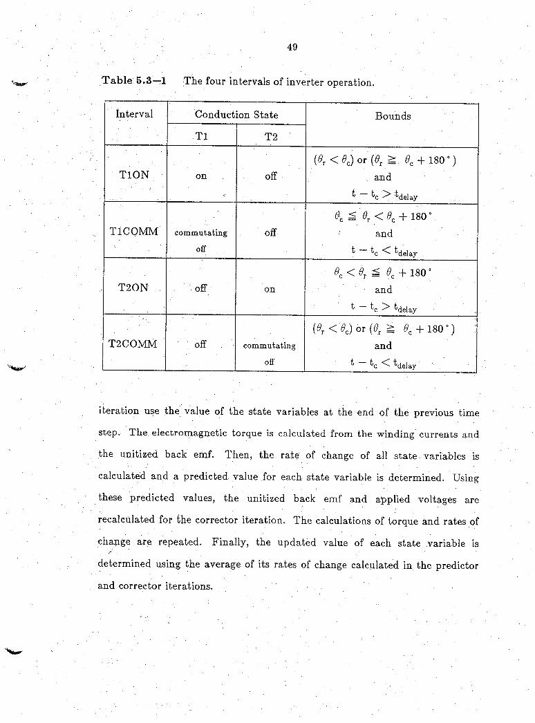
Table: 5 .3 —1 The four intervals of inverter operation.

Interval Conduction State Bounds

T l T2 ’

T lO N on off(0r < 0C) or [0I = 0c + 180 °)

and

fc — tC > delay

TlCQMM commutatingoff

off9C ^ 0T < 0C + 180 ’ .; and

t — tc < tdelay

T20N off on0C < 0T ^ Oc + 180°

andt — tc > tdelay

T2C0MM off commutatingoff

(0r < c) or (0r ^ 9C + 180 0 ) :and

I c ^ delay .

iteration use the value of the state variables at the end of the previous time

step. The electromagnetic torque is calculated from the winding currents and

the unitized back emf. Then, the rate of change of all state variables is

calculated and a predicted value for each state variable is determined. Using

these predicted values, the unitized back emf and applied voltages are

recalculated for the corrector iteration. The calculations of torque and rates of

change are repeated. Finally, the updated value of each state variable is

determined using the average of its rates of change calculated in the predictor

and corrector iterations.

5.4 An I-V Characteristic Model of the Inverter

The first method developed for calculating the applied stator voltages

utilizes piecewise-linear I-V characteristics to calculate the voltage across the

inverter switching elements (transistors and diodes). In this section, the I-V

characteristics (circuit models) for the transistors and diodes are presented.

The use of these models in the computer simulation is then discussed.

Equations in the following derivation are written for transistor T l and

diode DI, but are equally valid, with an appropriate change of subscripts, for

transistor T2 and diode D2. A switch voltage, Vswv is indicated in Fig. 5.3—1

as the voltage across the parallel combination of transistor T l and diode DI.

Expressions for the transistor voltage, vcel, and diode voltage, Vdl, will be

related to the switch voltage, vswl, which, in turn, is related to the applied

stator winding voltage, V1, by the equation

Tl Vdc vsw I (5,4-1 )

When a transistor is on (operated in saturation), it is modeled as a small

resistor connected between the collector and emitter terminals [6j. In this case,

the switch voltage, Tswl, which equals the transistor’s collector-to-emitter

voltage, is given by

Vswl *= Vcel = TsatI1 (5.4-2)

where rsat is the transistor’s collector-to-emitter saturation resistance and is

approximately 0.5 Cl. Because the switch voltage is also across the parallel

diode, it is restricted to values between the Zener and forward conduction

voltages of the diode as described in the subsequent discussion.

51

'h f When a transistor is off (operated in cutoff) or being commutated off, the

transistor is considered to be an open-circuit and the I-V characteristic of the

parallel diode determines the switch voltage. Thediodel-Vcharacteristicused

for the simulation is depicted in Fig. 5.4—1 with the slopes exaggerated for

clarity. In the diode’s reverse bias region of operation, between the negative

.......Zener voltage, — Vz, and the forward conduction voltage, Vb, the characteristic

has a positive slope of , and the diode voltage is related to the diode1Yev

(negative I-winding) current by

Vdi = - W i - f or ~ V z < v d i < v b ( 5 .4 -4 )

Diode voltages calculated using (5.4-4) which are'less than the negative Zener

voltage are clamped at vbl = — Vz, but generally this is not necessary because

the value selected for the Zener voltage prevents zenering except during

'*** commutation. Voltages above the forward conduction voltage are fixed at the

forward conduction voltage, vbl == Vb. From Fig. 5.3—I, the switch voltage

equals the opposite of the diode voltage, vswl = — vdl.

The model used for each transistor-diode pair in a given interval follows

directly from the conduction states listed in Table 5.3—1. For example, during

TlON, transistor T l is on and modeled by a transistor saturation resistance

while T2 is off and modeled by a diode reverse leakage resistance. By

symmetry, the models are exchanged during T20N. During the commutation

intervals, TlCOMM and T2C0MM, both transistor-diode pairs are modeled by

the diode I-V characteristic depicted in Fig. 5.4—I. Models fo rthe switching

elements are summarized in Table 5.4—I. After calculating the switch

voltages, the applied stator voltages are calculated by subtracting the switch

52

30V

F igure 5.4—1 Diode I-V characteristic used in the computer simulation,

voltages from the dc supply voltage.

Although the previous I-V characteristics of the transistors and diodes are

easily imp lehaented in a computer program, the resulting simulation requires

extremely small time steps. The need for a small time step can be explained

by considering the eigenvalues associated with the circuit shown Fig. 5.4—2,

This circuit, for the situation when transistor T l is on and T2 is off (TlON), is

a special case of the equivalent circuit in Fig. 5.3-1 and has a resistor

(rrev = 2 kH) replacing the reverse biased diode D2. The circuit eigenvalue

with largest modulus is on the order of 10 , indicating that simulation time

steps should be on the order 10 ^s. In fact, by trinl-nnd-error, 2.0x10 s was

found to the largest time step that did not result in a numerical instability

using the given predictor-corrector algorithm. Although larger time steps are

possible by decreasing the value of rrev, this has the adverse effect of permitting

• - ■ ' I

53-. ■ ;

T able 5 .4 -: I The I-V characteristic model for the switch voltages in each interval of inverter operation.

V - V . ... ■, SwitchVoltage V . ' ” : . ’ ‘ ' .- Interval■' '■ ■ ■ ; ■ ; ■ ' •' '■ - V • ■ ' ■ ■

■ ■ ■■ swl ' ■' vsw2 ■

' : v: TlO N vcel == rsat*l rsat*l vd2 rrev*2 if rr,yi. < V ,:: vvvvvvv ■ .V,. . Vr a l = - V b if FtalI1S - Vb >Ir3>I I f rrtrU i Vt

TlGOMM ” vdl rrev*l ^ rrev l ^ ~~yd2 — rrev 2 if r revi2> - V b■ . . ' . -Vdl - V 1 if FrtyI1 a v ,

>?:III3>I c. IIA I «r<

;■ ■T20N ydi IYeyi1 if rrevij < V Z yce2 YatY if rSat1Z > —Vb

■ ' • ". - ■ ' . ■■. - . ' ' ■ -V i1 ==Vz if Frevll= Vz vce2 = - V b IfF sa tizS -V b

■ ' ■' ; T2COMM vdl rrevb if 1YevY Vb Cl• r-HJIl3>I i f r rtyiz<Vs

-Yd1 - - V b if TrevI1 = — Vb — vd2 - Vz if FrtyI2 S V,

a, larger leakage current in the winding which, for practical purposes should be

zero. Decreasing the value of the coupling coefficient, k, also permits a larger

time step, but alters the nature of the electrodynamics. A second approach for

modeling the inverter is developed in the next section.

Operation of the actual jnptor-inverter system provided a benchmark for

Ithe simulation. Instantaneous winding currents and voltages for a motor

operating without external load,: Tl = Q, and at a (mechanical) speed of

3600 rpm (377 rad/s) were recorded experimentally. The dc supply voltage

required to maintain a no-load speed of 3600 rpm was determined through

trial-and-error as 6.3 V. Because the given motor is a four pole device, the

mechanical speed of 3600 rpm corresponds to an electrical angular frequency of

754 rad/s. Thus, the simulation was performed with CUr = 754 rad/s. The dc

rs .• Lss Lm-WV— i y s -

Lss Lm rs

OJm

P r

W V-rsat = 0.5 Cl O

-Vll

rrev 2kCt

Figure 5.4—2 Schematic diagram of the equivalent circuit for situation when T l is on and T2 is off.

supply voltage used in the simulation was the same as for the actual motor-

inverter. In particular, V^c = 6.3 V. Traces of the 1-winding current and

voltage from the simulation are shown along with the experimentally recorded

traces in Fig. 5.4-3. The simulation results compare well with the measured

waveforms. A more complete set of traces in Fig. 5.4—4 includes the 2-winding

current and voltage, as well as the electromagnetic torque, Te, and the (back)

emf.

55

0.60 0.40

I1V A 0.20 0.00

- 0.20

V1JV 0.0

-H (*-4.166 ms

i,, A 0.20

. . . ,. : '

' '-.-'-I

F igure 5.4—3 Comparison of traces from (a) simulation using I-V characteristics and (b) experimental measurement, for a motor operating at ;-Jr = 754 rad/s and T1 = 0.

Te, mN'm

Figure 5.4—4 I-V characteristic simulation results for motor operating at

5.5 A Functional Representation of the Inverter

In the so-called functional representation of the inverter, the switch

voltages, V s^ i and V sw 2 , are calculated at each time step using relationships

derived froip the voltage equations (5.2-2) and (5.2-3). In particular, modeling

of the inverter’s switching elements involves calculating the open-circuit

voltage which should appear across a transistor-diode pair whenever the

transistor is not on. By setting the switch voltage to this calculated open-

circuit value and determining the corresponding applied Stator voltage, the

appropriate winding current is maintained at or driven toward a value

corresponding to an open-circuit condition.

The schematic diagram of the finding equivalent circuit and inverter

shown in Fig. 5.3—1 will be considered again. In the following derivations, the

voltages across transistor T l and diode DI during each of the simulation

intervals areconsidered, but in order to simplify references, some of the

corresponding equations for transistor T2 and diode D2 are given without

derivation. ■■:: Vr-.-

In the functional model, the voltage applied to the stator winding whose

transistor is on must be determined before thq switch voltage of the transistor

which i$ -off *can be calculated. When a transistor is on (operated in

saturation), as during the interval T I ON, the transistor is modeled as a voltage

source connected between the collector and emitter terminals. In this case, the

switch voltage and transistor voltage are given by

‘ ; — Vcet ; (5 .5-1)

Likewise, during T20N, ;

_. _-T T satvsw2 ~ vce2 — v ce (5.5-2)

•where Y ^ t is the transistor collector-to-emitter saturation voltage and is

approximately 0.25 V. As with the I-V characteristic model, (5.4-1) is used to

calculate the applied stator winding voltage from the switch voltage.

Central to the functional representation of the inverter is the relationship

between the electric system dynamics and the switch voltage for the transistor

which is not on. The diode I-V characteristic places constraints on the switch

voltage, and it is convenient to write expressions for the diode voltage rather

than for the negative switch voltage. The voltage across diode Dl is obtained

from Kirchoffs voltage law applied to the loop containing diode DI, the 1-

winding, and the dc voltage supply, i.e.

. ■ :(5-5"3)

Substituting (5.2-2) f o r V 1 yields

VdI = ^Vi T LssPii —‘ tjmP*2 T pXm ^dc (5.5 4)

Solving (5.2-3) for pi2 and substituting into (5.5-4) yields

V dI = r si i , + b s s P i i - t SL[v 2 - r i2 + L mp i i + p X J + P'\n _ Vdc (5-5-5)' I ‘ -•

' ■ ' JJlCollecting terms and using the coupling coefficient, k, to replace —- and

. o / V ,../. . .. ■ ; / ■ . O - 1 j SS

d\.^ ~ W ~ to rePlace P \n yields

dX„vdi = V 1 + (I - k2)Lsspi1 - k(v2 - rsi2) + (I - k K -j^ 2- “ Vdc t5-5"6)

Similarly, for diode D2,

■ vd2 = rsi2 + (I — k2)Ls pi2 — k(vj — Vji1) - (I -k )a 'r^ - - V dc (5.5-7)■ . • ' T

Gonstraints on the diode voltage, vdl, expressed in (5.5-6) result from the

device’s physical characteristics. In particular, the diode voltage must remain

greater than the negative Zener voltage and below the forward conduction

voltage, - V z < vdl < Vj3, Equation (5.5-6) represents a general expression for

the Voltage developed across diode D l due to the electrical dynamics whenever

transistor T l is off or being commutated off. Specific simplifications of (5.5-6)

are made when considering each of the intervals T20N, T2COMM, and

TICOMM.

When transistor T l is off and T2 is on, namely the interval T2ON, the

function of T l and Dl is to prevent current from flowing in the 1-winding, i.e.

open-circuit the !-winding. In this case, I1 and Pi1 are zero and (5.5-6) may be

simplified to r --V

■ ':- 'W X :v: v. ■■ dXm ''W1--V-';-.VdI = ~ k(v2 ~ rsi2) + (I - k K — - - V dc

V V V - : \V>;- 'v V ' - v V d ^r - v . /

Likewise, during interval TlO N when T2 is off (5.5-7) reduces to

Vd2 = - M v 1 - T sI1) - ( I - k )H — ^ - V dc

(5.5-8)

(5.5-9)

Before evaluating (5.5-8), the 2-winding voltagej V2, is deterrnined using (5.5-2)

and the relationship V2 = Vdc — Vsw2. The other expressions on the right-hand

side Of (5.5-8) are readily established from simulation values. By applying the

stator voltage corresponding to the open-circuit diode voltage calculated with

(5.5-6), the value of the 1-winding current is held at zero throughout the

interval T20N. A different equation, however, must be used to calculate the

60

stator voltage necessary to drive the 1-winding current from a non-zero value

toward zero, i.e. commutate off transistor T l.

While transistor T l is being commutated off (interval TlCOMM), neither

the 1-winding current nor its time rate of change are zero. Thus, all terms on

the right-hand side of (5.5-6) contribute to the diode voltage, vdl, The

differentiation of the state variable q in the second term of (5.5-6), however,

makes use of this equation, as written, undesirable. Instead, an algebraic

relationship between the diode voltage and a predicted value for the 1-winding

current at the end of the time step will be derived from (5.5-6) by solving (5.5-

6) as a differential equation. Using the derived algebraic relationship, the diode

voltage which would drive the 1-winding current to zero at the end of the time

step is calculated. In order to avoid carrying complicated expressions through

the derivation of the hew expression for vdl, hew variables, Lc and vc, are

defined hs ■ ' ■

j SS

vc = Vdc + k(v2 - rsi2) - (I -k )w r d d T

(5.5-10)

(5.5-11)

All expressions on the right-hand side of (5.5-11) except V2 are readily-

established from simulation values at each time step. However, as T l is being

commutated off, the 1-winding current rapidly decreases to zero and a positive

voltage is induced in the 2-winding. This induced voltage forward biases diode

D2 whereupon V2 = Vb during this commutation interval. Given v2, Vc is

readily calculated from (5.5-11). The value of Vc obtained from (5.5-11) is

assumed constant throughout the time step. Using (5.5-10) and (5.5-11), (5.5-

61

6) may be rewritten as

PiI + ^ " iI = ^ “ (vg + vdi) (5.5-12)

This is a linear, first-order, inhomogeneous differential equation which is time-

invariant over a time step and can be solved in closed form. It is applicable

throughout the interval TlCOMM. At the start of each time step during

TlCOMM, the value of the !-winding current calculated during the previous

time step serves as the initial condition i1(t0) for (5.5-12). The solution to

(5.5-12) with the given initial condition and assuming vdl is constant is

ii(k —to) — b(to)eT (t — t0) j

+ — (vc + Vdl)r S

I - e (5.5-13)

Evaluating (5,5-13) at the end of the time step, whose length is h, yields

. Ib(h) = h M 6 c + — (vc + vdl)

r S

I - e~ t h (5.5-14)

Thus, the value of the 1-winding current at the end of a time step can be

predicted using (5.5-14). Because the purpose of the diode during

commutation is to drive the 1-winding current toward zero, vdl should be

calculated so that U1(Ii) = 0. Setting I1(Ii) = O in (5.5-14) and solving for vdl

yields

-^ /L cvdl = TsI1(I0) ! _ e- a / Lc — V„ (5.5-15)

Thus during TlCOMM, the value of the diode voltage, vdl, which, when

applied over the time step h, will drive the !-winding current to zero is

calculated using (5.5-15). If the calculated VtJi is less than —Vz, VtJ1 is set to

- V z to take into account zenering.

The applied voltages during the remaining interval, T2COMM, are

calculated in the same manner as during TlCOMM. The sequence of

calculations during all the intervals of inverter operation are summarized in

Table 5.5-1.

The use of the functional representation of the Inverter pertnits much

longer time steps than the I-V characteristic model. During the intervals

TlON and T20N, the time step can be as large as h = 500/zs, an improvement

of 250-fold. Eigenvalue analysis of the winding equivalent circuit with one

terminal open circuited (the effect of the functional representation) indicates

even longer time steps are possible, but further improvements are limited by

the higher space harmonics of the unitized back emf. During the intervals

TlCOMM and T2COMM, it is necessary to reduce the time step to 5 (Js in

order to accurately model the zenering of the inverter diodes.

Traces of the 1-winding current and voltage from a simulation at

<4 == 754 rad/s and Tl = 0 are shown along with expermentally recorded traces

in Fig. 5.5—1. A more complete set of traces in Fig. 5.5—2 includes the 2-

winding current and voltage as well as the electromagnetic torque, Te, and the

(back) emf.

T ab le 5.5—I Sequence of calculations during each interval of inverteroperation.

Interval Sequence of calculations

TlON' vcel = VcSeat

vI = Vdc - Vcei -dXm

Vd2 - - ^ v 1 - T sI1) - (I - k)wr - Vdc

v2 = Vdc + vd2

TlCOMM

V2 - V dc- V b ;

vc - Vdc + k’(v2 - T sI2) - (I - k)coT ^-r^/Lc . / r

Tdi - V 1W 1 ^ l l t 'V

if vdl < - V z then vdl = - Vz v r = V dc + vdl

; 'T ’20N;:' ;y _ ysatvce2 ... v ceV2 = V dc- V ce2 V

V- ■: . . dXmVdl - - k(v2 - rsi2) + (I - k )n ^ - Vdc

V1 = V dc + v d2

T2CPMM ;

V1 = Vdc - Vb :V ” dXm ■ ■

Vc = Vdc + k(Vi - TsI1) + (I - k)wr d0p-^/Lc

Vd2 - TsI2(O) i/L - Vc' I —- e rJi/L'if vd2 < - V z then vd2 = - V z 1v2 = Vdc + vd2

-H >-4.166ms

Figure 5.5—1 Com parison of traces from (a) sim ulation using functional representation and (b) experim ental m easurem ent, for a m otor operating at wr = 754 rad/s and T jj = 0.

65

V2, V o.o

Te, mN'm

4.0

2.0

o.o- 2.0

|*-4.166 ms

Figure 5.5—2 Functional representation simulation results for a motor operating at Wr = 754 rad/s and Tjj = 0.

CHAPTER 6

STEADY-STATE AND DYNAMIC SIMULATIONS

6.1 Introduction

The pulsating starting torque and large iiioment of inertia of the single-

phase brushless dc motor make it impractical for position-control or fast-

response speed-control applications. The motor is, however, well suited for

constant-speed (steady-state) operation. In this chapter, steady-state operation

of the motor is investigated using data produced by computer simulation. In

particular, a family of steady-state torque-speed and current-speed

characteristics are generated. F rom these characteristics, the normal operating

point for the motor is determined. Operation near this point is then simulate

and'.-the motor efficiency is determined. Finally, the computer simulation is

used to demonstrate the dynamic performance of the motor during starting.

6.2 Steady-State Gharacteristics

In order to investigate the steady-state performance of the motor,

electromagnetic torque-speed (Te—cur) and current-speed (I1- iCUr) characteristics

were generated using the computer simulation described in Chapter 5. Here, I1

represents the average current in the !-winding and Te is the average torque.

Families of the simulated Te- o;r and I1-CUr characteristics are depicted in

Fig. 6.2—1 and Fig. 6.2—2, respectively. The families consist of curves

corresponding to dc supply voltages ranging from 4 Y to 12 V. Each curve was

generated by simulating the motor at several constant rotor speeds (electrical

angular frequencies) ranging from 20rad/s to 1200rad/s and recording the

average electromagnetic torque and 1-winding current during one revolution.

The functional representation of the inverter was used in the. simulations in

order to reduce computation time; even so, this procedure for generating the

characteristics was computationally intensive.

The torque-speed characteristics in Fig. 6.2—1 are typical of a brushless dc

motor. In particular, the slopes of the curves are negative throughout the

region where rotor speed and electromagnetic torque are both positive (motor

action), and, at rotor speeds between stall and 377 rad/s, the characteristics are

nearly linear. The upward concavity for speeds above 377 rad/s is attributable

to commutation effects which become more prominent at higher speeds (larger

number of commutations per unit time). ;

Using the family of Te-Cur characteristics and manufacturer’s

specifications for running torque, the normal operating voltage for the motor

was established. The running torque is the combination of load torque, Tl,

and the windage and friction torque which is modeled as Bwr Manufacturer’s

specifications provided the normal running torque as 4.9 mN'm and rotor/speed

(electrical angular frequency) as 754 rad/s. In the steady state, the torque due

to inertial acceleration can be neglected and the electromagnetic torque

developed by the motor counters only the running torque. Thus, the point on

the Te-Wr characteristic whose ordinate is Te = 4.9mN-m and abscissa is

Tp, mN*m io

Figure 6.2—1 Torque-speed characteristics for Vdc = 4, 6,8,10, and 12 V.

Figtire 6.2—2 Current-speed characteristics^for V,jc — 4,6,8, IOj and 12V.

ooT = 754 rad/s corresponds to the normal operating point of the motor. This

point is indicated in Fig. 6.2-1. The dc supply voltage (applied stator winding

voltages) required for the motor to develop 4.9mN*m at 754 rad/s was

estimated as 8.3V by interpolation between the 8 and IOV curves in

Fig. 6.2—1. In practice, the applied stator winding voltages would be regulated

to maintain the appropriate operating point (rotor speed). That is, pulse

width modulation (PWM) would be employed to reduce a dc supply voltage of

12 V to an effective applied stator winding voltage of 8.3 V. Voltage reduction

through PWM is achieved by periodically switching the applied voltage to zero,

thereby reducing its average value. The length of time that zero voltage is

applied would be determined from a comparison of the measured rotor speed

with a reference speed. For purposes of simulation, however, it is assumed

that the dc supply voltage has been set to a constant value of 8.3 V and PWM

is not considered.

The motor operating at OJ1 =754 rad/s with Vdc = 8.3 V was simulated

with the inverter switching elements modeled by their T-V characteristics.

Resulting traces of the machine variables are given in Fig. 6.2—3. The most

notable aspects of the traces pertain to the winding currents. In particular, it

is noted that at the instant the winding currents are commutated, the value of

the two currents are nearly equal in magnitude but opposite in sign.

Considering the commutation of the winding current from the 1-winding to the

2-winding, i2 is zero prior to commutation and the flux linking both windings is

related only to T1 and the rotor permanent magnets. During the commutation

interval, iL decreases rapidly. But because the winding flux linkages have a

tendency to remain nearly constant throughout the commutation interval, the

decrease in ix requires a corresponding (negative) increase in i2. The increase in

i2 must have a negative sense because the mutual inductance is negative. The

forward-biased diode connected to the 2-winding provides the conduction path

for i2. After the commutation interval, i2 increases under the influence of the

applied stator voltage, V2, until the instantaneous back emf counters V2. The

instantaneous current, i2, decreases as the back emf reaches a maximum during

the latter part of the cycle. After reaching a maximum, the back emf

decreases and i2 again increases rapidly immediately prior to commutation. At

commutation, the cycle begins to repeat for the 1-winding current.

In addition to traces of the instantaneous machine variables for motor

operation at cc£ =?= 754 rad/s, torque-speed and Current-Speed characteristics for

Vdc= 8.3 V were generated. These characteristics are given in Fig. 6.2—4.

From these dhta, a plot of motor efficiency, 7], versus rotor speed can be

dbtained using the relatibnship: ':V W y ”'. f

. y * ■ S -W - ''. i- - ” ■■ y ' y . - 1 . : ' ' / • : : : . V . . - ' y V / "i V !

> ) - — - r ■ (6.2-1)

Where P in and Pout are the average input and output power, respectively. For

the brushless dc motor, the average input power is the product of the dc

supply voltage- (constant) and the average dc current drawn by motor. The

average dc current is obtained by doubling the I-winding current, I1, to

account for the second winding. The output power of the motor is the product

of electromagnetic torque with rotor mechanical speed. Because the motor is a

four-pole device, the rotor mechanical speed is equal to one-half the electrical

angular speed, i.e. -(Ur. Thus, the expression for efficiency becomes

-4 |*-4.166ms

Te, mN*m

Figure 6.2—3 Machine variables for motor operating with Wr = 754 rad/s and V cJc = 8.3 V.

Te, mN*m

Figure 6.2—4 Characteristics for YcJc = 8.3 Y (a) Te- e^ and (b) .Ij-W1,.

74

2 T ,H _ I T .H 2V,.!, J V dcI1

(6 .2- 2)

Using (6.2-2) and the data, from Fig. 6.2-4, the plot of efficiency given in

Fig. 6.2—5 was produced. The motor has an efficiency of 0.34 at

OOt = 754 rad/s, while a maximum efficiency of 0.37 is achieved around

u)T — 900 rad /s .

Tj 0.50

1131

F igure 6.2—5 Plot of motor efficiency for Vdc = 8.3 V.

6.3 S ta rtin g G haracteristics

The starting characteristics analyzed in Chapter 4 can be demonstrated

using the computer simulation of the motor. In order to accurately simulate

the starting characteristics, the cogging torque, which was omitted from the

75

expression for electromagnetic torque, is represented here as a position

dependent load torque. In particular, the form of the load torque is given by

>-'V--:,'-;/TL,:= lls in (2^ '-—'44 °) mN'm (6.3-1)

where 11 mN'm is the maximum cogging torque. The argument of sine

function in (6.3-1) follows directly from the plot of cogging torque in

Fig. 4.3—2. The rotor position must be initialized to a stable detent; the value

Ot ~ 292 0 is used. All other state variables are initialized to zero. During

starting of the actual motor, a maximum voltage of 12 Y is applied to the

stator windings, and in the simulation Vdc = 12 V. The proportionality

constant, B, for the windage and friction torque was calculated as 6.5 ulNbnrs

by dividing the manufacturer specified running torque by the specified rotor

speed. Using these data, the dynamic performance of the motor during

starting was simulated. Besulting traces of machine variables are given in

Big. h .3 -1 . V y ;h 'V;: v , v .■ 'V./.' Vv-''

These traces demonstrate many of the features hypothesized during the

analysis of the starting characteristics in Uhapter 4. > In particular, for the first

several revolutions after energizing the motor, the winding currents are nearly

rectangular and the the electromagnetic torque developed by the motor

resembles the derived static electromagnetic torque. The algebraic sum of the

electromagnetic, load, windage, and friction torques is labeled as Tnet in

Fig- 6.3.1. The net torque remains positive at all rotor positions and the motor

has a continuously positive acceleration.

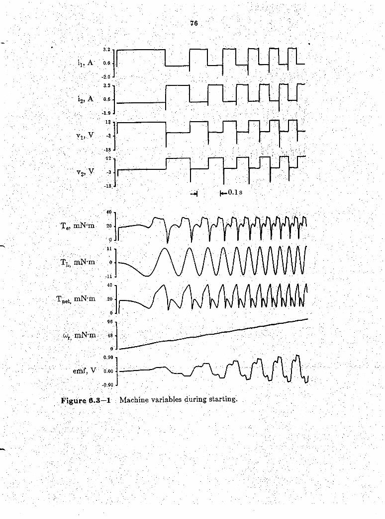
Vf':- r ..

- H K - O - I s

J lS L

_n_r

TLj mN-in o

F igure 6.3—1 Machine variables during starting.

CHAPTER 7

SUMMARY AND CONCLUSIONS

In this thesis, models of the permanent-magnet synchronous machine and

dc-to-ac inverter which comprise a single-phase brushless dc motor have been

developed. Central to the model of the brushless dc motor is the form of the

synchronous machine’s stator winding flux linkage due to the rotor permanent

magnets. The permanent-magnet component of stator flux linkage has been

derived analytically and compared with measured results revealing excellent

agreement. Two different mathematical models of the dc-to-ac inverter have

been established: one in which the current-voltage characteristics of the

inverter switching elements are incorporated; the second is a reduced model

which permits a more efficient computer simulation. Operation of the

brushless dc motor was simulated using each inverter model. Comparison of

simulation results with measurements of an actual motor-inverter system

indicate that the computer models are very accurate.

The starting response of the motor was analyzed using static

electromagnetic torque and cogging torque characteristics. The cogging torque

results from variations in the stator reluctance with respect to rotor position

and is accentuated intentionally by the asymmetry of the stator pole faces.

The cogging torque acts to drive the unexcited motor to a position at which

sufficient (static) electromagnetic torque is developed upon energization to

accelerate the motor. This method of ensuring that the motor develops

sufficient starting torque is well suited for the single-phase brushless dc motor.

LIST OF REFERENCES

LIST OF REFERENCES

[1] Takashi Kenjo, p crryq n en t-M a g n e t and Srush lesa D C M o to rs ,Caledon Press, 1985.

[2] M. R. Harris, "Brushless Motors - A Selective Review," P roc.First European Conferehce on Electrical Drives, Motors? and Controls pp. 84-90, July 1982.

[3] Paul C. Krause, A n u ly s is o f E lec tr ic M a ch in ery , McGraw Hill, 1986.

[4j Raymond DeCarlo, Class notes, 1987.

[5] James S. Vandergraft, In tro d u c tio n to N u m erica l C o m p u ta tio n s , Academic Press, 1978.

[6] William H. Hayt Jr. and Gerold W. Neudeck, E lec tro n ic C ircu itA n a ly s is and D esig n , Houghton Mifflin Co., 1984.