Analysis & PDE Vol 1 Issue 2, 2008 - msp.org
142
A NALYSIS & PDE A NALYSIS & PDE A NALYSIS & PDE A NALYSIS & PDE A NALYSIS & PDE A NALYSIS & PDE A NALYSIS & PDE A NALYSIS & PDE A NALYSIS & PDE A NALYSIS & PDE A NALYSIS & PDE A NALYSIS & PDE A NALYSIS & PDE A NALYSIS & PDE A NALYSIS & PDE A NALYSIS & PDE A NALYSIS & PDE A NALYSIS & PDE A NALYSIS & PDE A NALYSIS & PDE A NALYSIS & PDE A NALYSIS & PDE A NALYSIS & PDE A NALYSIS & PDE A NALYSIS & PDE A NALYSIS & PDE A NALYSIS & PDE A NALYSIS & PDE A NALYSIS & PDE A NALYSIS & PDE A NALYSIS & PDE A NALYSIS & PDE A NALYSIS & PDE A NALYSIS & PDE A NALYSIS & PDE A NALYSIS & PDE A NALYSIS & PDE A NALYSIS & PDE A NALYSIS & PDE A NALYSIS & PDE A NALYSIS & PDE A NALYSIS & PDE A NALYSIS & PDE A NALYSIS & PDE A NALYSIS & PDE A NALYSIS & PDE A NALYSIS & PDE A NALYSIS & PDE A NALYSIS & PDE A NALYSIS & PDE A NALYSIS & PDE A NALYSIS & PDE A NALYSIS & PDE A NALYSIS & PDE A NALYSIS & PDE A NALYSIS & PDE A NALYSIS & PDE A NALYSIS & PDE A NALYSIS & PDE A NALYSIS & PDE A NALYSIS & PDE A NALYSIS & PDE A NALYSIS & PDE A NALYSIS & PDE A NALYSIS & PDE A NALYSIS & PDE A NALYSIS & PDE A NALYSIS & PDE A NALYSIS & PDE A NALYSIS & PDE A NALYSIS & PDE A NALYSIS & PDE A NALYSIS & PDE A NALYSIS & PDE Volume 1 No. 2 2008 Volume 1 No. 2 2008 Volume 1 No. 2 2008 Volume 1 No. 2 2008 Volume 1 No. 2 2008 Volume 1 No. 2 2008 Volume 1 No. 2 2008 Volume 1 No. 2 2008 Volume 1 No. 2 2008 Volume 1 No. 2 2008 Volume 1 No. 2 2008 Volume 1 No. 2 2008 Volume 1 No. 2 2008 Volume 1 No. 2 2008 Volume 1 No. 2 2008 Volume 1 No. 2 2008 Volume 1 No. 2 2008 Volume 1 No. 2 2008 Volume 1 No. 2 2008 Volume 1 No. 2 2008 Volume 1 No. 2 2008 Volume 1 No. 2 2008 Volume 1 No. 2 2008 Volume 1 No. 2 2008 Volume 1 No. 2 2008 Volume 1 No. 2 2008 Volume 1 No. 2 2008 Volume 1 No. 2 2008 Volume 1 No. 2 2008 Volume 1 No. 2 2008 Volume 1 No. 2 2008 Volume 1 No. 2 2008 Volume 1 No. 2 2008 Volume 1 No. 2 2008 Volume 1 No. 2 2008 Volume 1 No. 2 2008 Volume 1 No. 2 2008 Volume 1 No. 2 2008 Volume 1 No. 2 2008 Volume 1 No. 2 2008 Volume 1 No. 2 2008 Volume 1 No. 2 2008 Volume 1 No. 2 2008 Volume 1 No. 2 2008 Volume 1 No. 2 2008 Volume 1 No. 2 2008 Volume 1 No. 2 2008 Volume 1 No. 2 2008 Volume 1 No. 2 2008 Volume 1 No. 2 2008 Volume 1 No. 2 2008 Volume 1 No. 2 2008 Volume 1 No. 2 2008 Volume 1 No. 2 2008 Volume 1 No. 2 2008 Volume 1 No. 2 2008 Volume 1 No. 2 2008 Volume 1 No. 2 2008 Volume 1 No. 2 2008 Volume 1 No. 2 2008 Volume 1 No. 2 2008 Volume 1 No. 2 2008 Volume 1 No. 2 2008 Volume 1 No. 2 2008 Volume 1 No. 2 2008 Volume 1 No. 2 2008 Volume 1 No. 2 2008 Volume 1 No. 2 2008 Volume 1 No. 2 2008 Volume 1 No. 2 2008 Volume 1 No. 2 2008 Volume 1 No. 2 2008 Volume 1 No. 2 2008 Volume 1 No. 2 2008 mathematical sciences publishers
Transcript of Analysis & PDE Vol 1 Issue 2, 2008 - msp.org

ANALYSIS & PDEVolume 1 No. 2 2008
AN
ALY
SIS&
PDE
Vol.1,N
o.2A
NA
LYSIS
&PD
EVol.1,
No.2
2008
ANALYSIS & PDEANALYSIS & PDEANALYSIS & PDEANALYSIS & PDEANALYSIS & PDEANALYSIS & PDEANALYSIS & PDEANALYSIS & PDEANALYSIS & PDEANALYSIS & PDEANALYSIS & PDEANALYSIS & PDEANALYSIS & PDEANALYSIS & PDEANALYSIS & PDEANALYSIS & PDEANALYSIS & PDEANALYSIS & PDEANALYSIS & PDEANALYSIS & PDEANALYSIS & PDEANALYSIS & PDEANALYSIS & PDEANALYSIS & PDEANALYSIS & PDEANALYSIS & PDEANALYSIS & PDEANALYSIS & PDEANALYSIS & PDEANALYSIS & PDEANALYSIS & PDEANALYSIS & PDEANALYSIS & PDEANALYSIS & PDEANALYSIS & PDEANALYSIS & PDEANALYSIS & PDEANALYSIS & PDEANALYSIS & PDEANALYSIS & PDEANALYSIS & PDEANALYSIS & PDEANALYSIS & PDEANALYSIS & PDEANALYSIS & PDEANALYSIS & PDEANALYSIS & PDEANALYSIS & PDEANALYSIS & PDEANALYSIS & PDEANALYSIS & PDEANALYSIS & PDEANALYSIS & PDEANALYSIS & PDEANALYSIS & PDEANALYSIS & PDEANALYSIS & PDEANALYSIS & PDEANALYSIS & PDEANALYSIS & PDEANALYSIS & PDEANALYSIS & PDEANALYSIS & PDEANALYSIS & PDEANALYSIS & PDEANALYSIS & PDEANALYSIS & PDEANALYSIS & PDEANALYSIS & PDEANALYSIS & PDEANALYSIS & PDEANALYSIS & PDEANALYSIS & PDEANALYSIS & PDEVolume 1 No. 2 2008Volume 1 No. 2 2008Volume 1 No. 2 2008Volume 1 No. 2 2008Volume 1 No. 2 2008Volume 1 No. 2 2008Volume 1 No. 2 2008Volume 1 No. 2 2008Volume 1 No. 2 2008Volume 1 No. 2 2008Volume 1 No. 2 2008Volume 1 No. 2 2008Volume 1 No. 2 2008Volume 1 No. 2 2008Volume 1 No. 2 2008Volume 1 No. 2 2008Volume 1 No. 2 2008Volume 1 No. 2 2008Volume 1 No. 2 2008Volume 1 No. 2 2008Volume 1 No. 2 2008Volume 1 No. 2 2008Volume 1 No. 2 2008Volume 1 No. 2 2008Volume 1 No. 2 2008Volume 1 No. 2 2008Volume 1 No. 2 2008Volume 1 No. 2 2008Volume 1 No. 2 2008Volume 1 No. 2 2008Volume 1 No. 2 2008Volume 1 No. 2 2008Volume 1 No. 2 2008Volume 1 No. 2 2008Volume 1 No. 2 2008Volume 1 No. 2 2008Volume 1 No. 2 2008Volume 1 No. 2 2008Volume 1 No. 2 2008Volume 1 No. 2 2008Volume 1 No. 2 2008Volume 1 No. 2 2008Volume 1 No. 2 2008Volume 1 No. 2 2008Volume 1 No. 2 2008Volume 1 No. 2 2008Volume 1 No. 2 2008Volume 1 No. 2 2008Volume 1 No. 2 2008Volume 1 No. 2 2008Volume 1 No. 2 2008Volume 1 No. 2 2008Volume 1 No. 2 2008Volume 1 No. 2 2008Volume 1 No. 2 2008Volume 1 No. 2 2008Volume 1 No. 2 2008Volume 1 No. 2 2008Volume 1 No. 2 2008Volume 1 No. 2 2008Volume 1 No. 2 2008Volume 1 No. 2 2008Volume 1 No. 2 2008Volume 1 No. 2 2008Volume 1 No. 2 2008Volume 1 No. 2 2008Volume 1 No. 2 2008Volume 1 No. 2 2008Volume 1 No. 2 2008Volume 1 No. 2 2008Volume 1 No. 2 2008Volume 1 No. 2 2008Volume 1 No. 2 2008Volume 1 No. 2 2008
mathematical sciences publishers

Analysis & PDEpjm.math.berkeley.edu/apde
EDITORS
EDITOR-IN-CHIEF
Maciej ZworskiUniversity of California
Berkeley, USA
BOARD OF EDITORS
Michael Aizenman Princeton University, USA Nicolas Burq Universite Paris-Sud 11, [email protected] [email protected]
Luis A. Caffarelli University of Texas, USA Sun-Yung Alice Chang Princeton University, [email protected] [email protected]
Michael Christ University of California, Berkeley, USA Charles Fefferman Princeton University, [email protected] [email protected]
Ursula Hamenstaedt Universitat Bonn, Germany Nigel Higson Pennsylvania State Univesity, [email protected] [email protected]
Vaughan Jones University of California, Berkeley, USA Herbert Koch Universitat Bonn, [email protected] [email protected]
Izabella Laba University of British Columbia, Canada Gilles Lebeau Universite de Nice Sophia Antipolis, [email protected] [email protected]
Laszlo Lempert Purdue University, USA Richard B. Melrose Massachussets Institute of Technology, [email protected] [email protected]
Frank Merle Universite de Cergy-Pontoise, France William Minicozzi II Johns Hopkins University, [email protected] [email protected]
Werner Muller Universitat Bonn, Germany Yuval Peres University of California, Berkeley, [email protected] [email protected]
Gilles Pisier Texas A&M University, and Paris 6 Tristan Riviere ETH, [email protected] [email protected]
Igor Rodnianski Princeton University, USA Wilhelm Schlag University of Chicago, [email protected] [email protected]
Sylvia Serfaty New York University, USA Yum-Tong Siu Harvard University, [email protected] [email protected]
Terence Tao University of California, Los Angeles, USA Michael E. Taylor Univ. of North Carolina, Chapel Hill, [email protected] [email protected]
Gunther Uhlmann University of Washington, USA Andras Vasy Stanford University, [email protected] [email protected]
Dan Virgil Voiculescu University of California, Berkeley, USA Steven Zelditch Johns Hopkins University, [email protected] [email protected]
PRODUCTION
[email protected] Ney de Souza, Production Manager Sheila Newbery, Senior Production Editor Silvio Levy, Senior Production Editor
See inside back cover or pjm.math.berkeley.edu/apde for submission instructions.
Regular subscription rate for 2008: $180.00 a year ($120.00 electronic only).Subscriptions, requests for back issues from the last three years and changes of subscribers address should be sent to Mathematical SciencesPublishers, Department of Mathematics, University of California, Berkeley, CA 94720-3840, USA.
Analysis & PDE, at Mathematical Sciences Publishers, Department of Mathematics, University of California, Berkeley, CA 94720-3840 ispublished continuously online. Periodical rate postage paid at Berkeley, CA 94704, and additional mailing offices.
PUBLISHED BYmathematical sciences publishers
http://www.mathscipub.orgA NON-PROFIT CORPORATION
Typeset in LATEXCopyright ©2008 by Mathematical Sciences Publishers
ANALYSIS AND PDEVol. 1, No. 2, 2008
MICROLOCAL PROPAGATION NEAR RADIAL POINTS ANDSCATTERING FOR SYMBOLIC POTENTIALS OF ORDER ZERO
ANDREW HASSELL, RICHARD MELROSE AND ANDRÁS VASY
In this paper, the scattering and spectral theory of H =1g + V is developed, where 1g is the Laplacianwith respect to a scattering metric g on a compact manifold X with boundary and V ∈ C∞(X) is real;this extends our earlier results in the two-dimensional case. Included in this class of operators are per-turbations of the Laplacian on Euclidean space by potentials homogeneous of degree zero near infinity.Much of the particular structure of geometric scattering theory can be traced to the occurrence of radialpoints for the underlying classical system. In this case the radial points correspond precisely to criticalpoints of the restriction, V0, of V to ∂X and under the additional assumption that V0 is Morse a functionalparameterization of the generalized eigenfunctions is obtained.
The main subtlety of the higher dimensional case arises from additional complexity of the radialpoints. A normal form near such points obtained by Guillemin and Schaeffer is extended and refined, al-lowing a microlocal description of the null space of H −σ to be given for all but a finite set of “threshold”values of the energy; additional complications arise at the discrete set of “effectively resonant” energies.It is shown that each critical point at which the value of V0 is less than σ is the source of solutions ofHu = σu. The resulting description of the generalized eigenspaces is a rather precise, distributional,formulation of asymptotic completeness. We also derive the closely related L2 and time-dependentforms of asymptotic completeness, including the absence of L2 channels associated with the nonminimalcritical points. This phenomenon, observed by Herbst and Skibsted, can be attributed to the fact that theeigenfunctions associated to the nonminimal critical points are “large” at infinity; in particular they aretoo large to lie in the range of the resolvent R(σ ± i0) applied to compactly supported functions.
1. Introduction 1282. Radial points 1353. Microlocal normal form 1404. Microlocal solutions 1555. Test modules 1576. Effectively nonresonant operators 1657. Effectively resonant operators 1748. From microlocal to approximate eigenfunctions 1779. Microlocal Morse decomposition 17910. L2-parameterization of the generalized eigenspaces 181
MSC2000: primary 35P25; secondary 81U99.Keywords: radial point, scattering metric, degree zero potential, asymptotics of generalized eigenfunctions, microlocal Morse
decomposition, asymptotic completeness.Hassell was supported in part by an Australian Research Council Fellowship. Melrose was supported in part by the NationalScience Foundation under grant #DMS-0408993. Vasy was supported in part by the National Science Foundation under grant#DMS-0201092, a Clay Research Fellowship and a Fellowship from the Alfred P. Sloan Foundation.
127

128 ANDREW HASSELL, RICHARD MELROSE AND ANDRÁS VASY
11. Time-dependent Schrodinger equation 186Appendix: Errata for [Hassell et. al 2004] 193Acknowledgement 195References 195
1. Introduction
In this paper, which is a continuation of [Hassell et al. 2004] (sometimes referred to as Part I) scatteringtheory is developed for symbolic potentials of order zero. The general setting is the same as in Part I,consisting of a compact manifold with boundary, X , equipped with a scattering metric, g, and a realpotential, V ∈ C∞(X). Recall that such a scattering metric on X is a smooth metric in the interior of Xtaking the form
g =dx2
x4 +hx2 (1–1)
near the boundary, where x is a boundary defining function and h is a smooth cotensor which restrictsto a metric on {x = 0} = ∂X . This makes the interior, X◦, of X a complete manifold which is asymptot-ically flat and is metrically asymptotic to the large end of a cone, since in terms of the singular normalcoordinate r = x−1, the leading part of the metric at the boundary takes the form dr2
+ r2h(y, dy).In the compactification of X◦ to X , ∂X corresponds to the set of asymptotic directions of geodesics.In particular, this setting subsumes the case of the standard metric on Euclidean space, or a compactlysupported perturbation of it, with a potential which is a classical symbol of order zero, hence not decayingat infinity but rather with leading term which is asymptotically homogeneous of degree zero. The studyof the scattering theory for such potentials was initiated by Herbst [1991].
Let V0 ∈ C∞(∂X) be the restriction of V to ∂X , and denote by Cv(V ) the set of critical values of V0.It is shown in [Hassell et al. 2004] that the operator H =1g + V (where the Laplacian is normalized tobe positive) is essentially self-adjoint with continuous spectrum occupying [min V0,∞). There may bediscrete spectrum of finite multiplicity in (− minX V,max V0] with possible accumulation points only atCv(V ). To obtain finer results, it is natural to assume, as we do throughout this paper unless otherwisenoted, that V0 is a Morse function, that is, has only nondegenerate critical points; in particular Cv(V ) isthen a finite set; by definition this is the set of threshold energies, or thresholds.
From the microlocal point of view scattering theory is largely about the study of radial points, that is,the points in the cotangent bundle where the Hamilton vector field is a multiple of the radial vector field(that is, the vector field A =
∑i zi∂zi on Euclidean space, where (z1, . . . , zn)∈ Rn). These correspond in
the classical dynamical system to the places where the particle is moving either in purely incoming or out-going sense. In scattering theory for potentials decaying at infinity, there is a radial point for each point onthe sphere at infinity; thus there is a manifold of radial points and the behaviour of the flow in a neighbour-hood of these points is rather simple, either attracting (at the outgoing radial surface) or repelling (at theincoming radial surface) in the transverse direction. Estimates involving commutation with the radial vec-tor field A multiplied by suitable powers of |z| and perhaps additional microlocalizing operators, are usu-ally sufficient to control the behaviour of generalized eigenfunctions. These are known as Mourre-typeestimates and play a fundamental role in conventional scattering theory. In the present case, assuming V0
is a Morse function, the radial points are isolated and occur in pairs, one pair (incoming/outgoing) for each
MICROLOCAL PROPAGATION NEAR RADIAL POINTS AND SCATTERING FOR SYMBOLIC POTENTIALS 129
critical point of V0. The linearized Hamiltonian flow at the radial points is rather more complicated since itdepends on the Hessian of V0 at the critical point, which is arbitrary apart from being nondegenerate. Thismakes the higher dimensional case more intricate than the case dim X = 2 which we treated in [Hassellet al. 2004]. Correspondingly one needs more elaborate commutator estimates in order to control the be-haviour of generalized eigenfunctions. We give a rather general and complete analysis of the regularity ofsolutions of Pu =0 in a microlocal neighbourhood of a radial point of P , using the concept of a test mod-ule of operators. This is a family of pseudodifferential operators which is a module over the zero-orderoperators, contains P , and is closed under commutation. By choosing a test module closely tailored to theHamilton flow of P near the radial point we are able to produce enough positive-commutator estimatesto parametrize the microlocal solutions of Pu = 0. The construction of appropriate test modules (whichcan be thought of as simply an effective bookkeeping device for keeping track of a rather intricate set ofcommutator estimates) to analyze general radial points is the main technical innovation of this paper.
The general study of radial points was initiated by Guillemin and Schaeffer [1977]. This was done in aslightly different context, where P is a standard pseudodifferential operator with homogeneous principalsymbol and a radial point is one where the Hamilton vector field is a multiple of the vector field
∑i ξi∂ξi
generating dilations in the cotangent space. This setting is completely equivalent to ours, via conjugationby a “local Fourier Transform” (see Section 3.1). They analyzed the situation in the nonresonant case.We refine their analysis by treating the resonant case, which is crucial in our application since we havea family of operators parametrized by the energy level, and the closure of the set of energies which giverise to resonant radial points may have nonempty interior. Moreover, we show that our parametrization ofmicrolocal solutions is smooth except at a set of “effectively resonant” energies which is always discrete.
Bony, Fujiie, Ramond and Zerzeri [Bony et al. 2007] have studied the microlocal kernel of pseudodif-ferential operators at a hyperbolic fixed point, corresponding, in our setting, to a radial point associatedto a local maximum of V0. Their results partially overlap ours, being most closely related to [Hassellet al. 2004, Section 10] and [Hassell et al. 2001].
1.1. Previous results. The Euclidean setting described above was first studied by Herbst [1991], whoshowed that any finite energy solution of the time dependent Schrodinger equation, so u = e−i t H f withf ∈ L2(Rn), can concentrate, in an L2 sense, asymptotically as t → ∞ only in directions which arecritical points of V0. This was subsequently refined by Herbst and Skibsted [2008], who showed thatsuch concentration can only occur near local minima of V0. In contrast, solutions of the classical flowcan concentrate near any critical point of V0.
Asymptotic completeness has been studied by Agmon, Cruz and Herbst [1999], by Herbst and Skib-sted [1999; 2008; 2004] and the present authors in [Hassell et al. 2004]. Agmon, Cruz and Herbstshowed asymptotic completeness for sufficiently high energies, while Herbst and Skibsted extended thisto all energies except for an explicitly given union of bounded intervals; in the two dimensional case,they showed asymptotic completeness for all energies. These results were obtained by time-dependentmethods. On the other hand the principal result of [Hassell et al. 2004] involves a precise description ofthe generalized eigenspaces of H
E−∞(σ )= {u ∈ C−∞(X); (H − σ)u = 0};
note that the space of “extendible distributions” C−∞(X) is the analogue of tempered distributions

130 ANDREW HASSELL, RICHARD MELROSE AND ANDRÁS VASY
and reduces to it in case X is the radial compactification of Rn . Thus we are studying all temperedeigenfunctions of H . Let us recall these results in more detail.
For any σ /∈ Cv(V ) the space Epp(σ ) of L2 eigenfunctions is finite dimensional, and reduces tozero except for σ in a discrete (possibly empty) subset of [minX V,max V0] \ Cv(V ). It is always thecase that Epp(σ ) ⊂ C∞(X) consists of rapidly decreasing functions. Hence E−∞
ess (σ ) ⊂ E−∞(σ ), theorthocomplement of Epp(σ ), is well defined for σ /∈ Cv(V ). Furthermore, as shown in the Euclidean caseby Herbst [1991], the resolvent, R(σ ) of H , acting on this orthocomplement, has a limit, R(σ ± i0), on[min V0,∞)\Cv(V ) from above and below. The subspace of “smooth” eigenfunctions is then defined as
E∞
ess(σ )= Sp(σ )(C∞(X) Epp(σ )
)⊂ E−∞(σ ), Sp(σ )≡
12π i
(R(σ + i0)− R(σ − i0)
). (1–2)
In factE∞
ess(σ )⊂
⋂ε>0
x−1/2−εL2(X).
An alternative characterization of E∞ess(σ ) can be given in terms of the scattering wavefront set at the
boundary of X .The scattering cotangent bundle, scT ∗X , of X is naturally isomorphic to the cotangent bundle over
the interior of X , and indeed globally isomorphic to T ∗X by a nonnatural isomorphism; the naturalidentification exhibits both “compression” and “rescaling” at the boundary. If (x, y) are local coordinatesnear a boundary point of X , with x a boundary defining function, then linear coordinates (ν, µ) are definedon the scattering cotangent bundle by requiring that q ∈
scT ∗X be written as
q = −νdxx2 +
∑i
µidyi
x, ν ∈ R, µ ∈ Rn−1. (1–3)
This makes (ν, µ) dual to the basis (−x2∂x , x∂yi ) of vector fields which form an approximately unitlength basis, uniformly up to the boundary, for any scattering metric. In Euclidean space, ν is dual to ∂r
and µi is dual to the constant-length angular derivative r−1∂yi . In the analysis of the microlocal aspectsof H − σ , in part for compatibility with [Guillemin and Schaeffer 1977], it is convenient pass to anoperator “of first order” by multiplying H − σ by x−1, that is, to replace it by
P = P(σ )= x−1(H − σ).
The classical dynamical system giving the behaviour of particles, asymptotically near ∂X , moving underthe influence of the potential corresponds to “the bicharacteristic vector field,” see (2–3), determined bythe boundary symbol, p, of P . This vector field is defined on scT ∗
∂X X , which is to say on scT ∗X at, and tan-gent to, the boundary scT ∗
∂X X =scT ∗X∩{x =0}. It has the property that ν is nondecreasing under the flow;
we refer to points (y, ν, µ) where µ= 0 as incoming if ν < 0 and outgoing if ν > 0. What is important inunderstanding the behaviour of the null space of P , that is, tempered distributions, u, satisfying Pu = 0,is bicharacteristic flow inside {p = 0, x = 0}, a submanifold to which it is tangent. The only criticalpoints of the flow are at points (y, ν, 0) where y is a critical point of P and ν = ±
√σ − V (y). Thus, the
only possible asymptotic escape directions of classical particles under the influence of the potential Vare the finite number of critical points of V0. Moreover, only the local minima are stable; the others haveunstable directions according to the number of unstable directions as a critical point of V0 : ∂X −→ R.

MICROLOCAL PROPAGATION NEAR RADIAL POINTS AND SCATTERING FOR SYMBOLIC POTENTIALS 131
The classical dynamics of p and the quantum dynamics of P are linked via the scattering wavefrontset. Let u ∈ C−∞(X) be a tempered distribution on X (that is, in the dual space of C∞(X;�)). The partof the scattering wavefront set, WFsc(u), of u lying over the boundary {x = 0}, which is all that is ofinterest here, is a closed subset of scT ∗
∂X X which measures the linear oscillations (Fourier modes, in thecase of Euclidean space) present in u asymptotically near boundary points; see [Melrose 1994] for theprecise definition. We shall also need to use the scattering wavefront set WFs
sc(u)with respect to the spacex s L2(X) which measures the microlocal regions where u fails to be in x s L2(X). There is a propagationtheorem for the scattering wavefront set in the style of the theorem of Hormander in the standard setting;if Pu ∈ C∞(X), then the scattering wavefront set of u is contained in {p = 0} and is invariant underthe bicharacteristic flow of P; see [Melrose 1994]. In particular, generalized eigenfunctions of u havescattering wavefront set invariant under the bicharacteristic flow of P . Note that the elliptic part of thisstatement is already a uniform version of the smoothness of solutions.
In view of this propagation theorem, it is possible to consider where generalized eigenfunctions“originate”, although the direction of propagation is fixed by convention. Let us say that a generalizedeigenfunction originates at a radial point q, if q ∈ WFsc(u) and if WFsc(u) is contained in the forwardflowout 8+(q) of q; thus each point in WFsc(u) can be reached from q by travelling along curves thatare everywhere tangent to the flow and with ν nondecreasing along the curve, so allowing the possibilityof passing through radial points, where the flow vanishes, on the way. In Part I of this paper we showed,in the two-dimensional case and provided the eigenvalue σ is a nonthreshold value:
• Every L2 eigenfunction is in C∞(X).• Every nontrivial generalized eigenfunction pairing to zero with the L2 eigenspace fails to be in
x−1/2L2(X).• There are generalized eigenfunctions originating at each of the incoming radial points in {p = 0},
that is, at each critical point of V0 with value less than σ .• There are fundamental differences between the behaviour of eigenfunctions near a local minimum
and at other critical points. The radial point corresponding to a local minimum is always an isolatedpoint of the scattering wavefront set for some nontrivial eigenfunction. For other critical points, thescattering wavefront set necessarily propagates and in generic situations each nontrivial generalizedeigenfunction is singular at some minimal radial point.
• A generalized eigenfunction, u, with an isolated point in its scattering wavefront set, necessarily aradial point corresponding to a local minimum of V0, has a complete asymptotic expansion there.The expansion is determined by its leading term, which is a Schwartz function of n − 1 variables.The resulting map extends by continuity to an injective map from E∞
ess(σ ) into⊕
q L2(Rn−1), wherethe direct sum is over local minima of V0 with value less than the energy σ .
• The space E0ess(σ ), consisting of those generalized eigenfunctions which are in x−1/2L2 microlocally
near {ν = 0}, is a Hilbert space and the map above extends to a unitary isomorphism, M+(σ ), fromE0
ess(σ ) to⊕
q L2(Rn−1). A similar map M−(σ ) can be defined by reversal of sign or complexconjugation and the scattering matrix for P = P(σ ) at energy σ may be written
S(σ )= M+(σ )M−1−(σ ).
In this paper we extend these results to higher dimensions.

132 ANDREW HASSELL, RICHARD MELROSE AND ANDRÁS VASY
1.2. Results and structure of the paper. We treat this problem by microlocal methods. Thus, the “classi-cal” system, consisting of the bicharacteristic vector field, plays a dominant role. The main step involvesreducing this vector field to an appropriate normal form in a neighbourhood of each of its zeroes, whichare just the radial points. Nondegeneracy of the critical points of V0 implies nondegeneracy of thelinearization of the bicharacteristic vector field at the corresponding radial points. If there are no reso-nances, Sternberg’s Linearization Theorem, following an argument of Guillemin and Schaeffer, allowsthe bicharacteristic vector field to be reduced to its linearization by a contact transformation of scT ∗
∂X X .At the quantum level this means that conjugation by a (scattering) Fourier integral operator, associatedto this contact transformation, microlocally replaces P by an operator with principal symbol in normalform. For this normal form we construct “test modules” of pseudodifferential operators and analyze thecommutators with the transformed operator. Modulo lower order terms, the operator itself becomes aquadratic combination of elements of the test module. Just as in Part I, we use the resulting system ofregularity constraints to determine the microlocal structure of the eigenfunctions and ultimately showthe existence of asymptotic expansions for eigenfunctions with some additional regularity.
However, the problem of resonances cannot be avoided. Even for a fixed operator and fixed criticalpoint, the closure of the set of values of σ for which resonances occur may have nonempty interior.Such resonances prevent the reduction of the bicharacteristic vector field to its linearization, and henceof the symbol of P to an associated model, although partial reductions are still possible. In general it isnecessary to allow many more terms in the model. Fortunately most of these terms are not relevant tothe construction of the test modules and to the derivation of the asymptotic expansions. We distinguishbetween “effectively nonresonant” energies, where the additional resonant terms are such that the defini-tion of the test modules, now only to finite order, proceeds much as before and the “effectively resonant”energies, where this is not the case. Ultimately, we analyze the regularity of solutions at all (nonthreshold)energies. Near effectively nonresonant energies, smoothness of families of eigenfunctions may still bereadily shown. Effectively resonant energies are harder to analyze, but the set of these is shown tobe discrete. In any case, the space of microlocal eigenfunctions is parameterized at all nonthresholdenergies. At effectively resonant energies the problems arising from the failure of the direct analogue ofSternberg’s linearization are overcome by showing that, to an appropriate finite order, the operator maybe reduced to a nonquadratic function of the test module.
In outline, the discussion proceeds as follows. In Sections 2–4 we study radial points. This is a generalmicrolocal study except that we work under the assumption that the symplectic map associated to thelinearization of the flow at each radial point (see Lemma 2.5) has no 4-dimensional irreducible invariantsubspaces; this assumption is always fulfilled in the case of our operator 1+ V − σ . The main result isTheorem 3.11 in which the operator is microlocally conjugated to a linear vector field plus certain “errorterms”. In the nonresonant case the error terms can be made to vanish identically, while in the effectivelynonresonant case the error terms have a good property with respect to a test module of pseudodifferentialoperators, namely they can be expressed as a positive power xε , ε > 0, times a power of the module. Inthe effectively resonant case this is no longer possible and we must allow “genuinely” resonant terms,but the set of effectively resonant energies is discrete in the parameter σ in all dimensions.
We then turn in Sections 5–7 to studying microlocal eigenfunctions which are microlocally outgoingat a given radial point q . The main result here is Theorem 6.7 (or Theorem 7.3 in the effectively resonantcase) which gives a parameterization of such microlocal eigenfunctions. For a minimal radial point, they

MICROLOCAL PROPAGATION NEAR RADIAL POINTS AND SCATTERING FOR SYMBOLIC POTENTIALS 133
are parameterized by S(Rn−1), Schwartz functions of n − 1 variables, for a maximal radial point theyare parameterized by formal power series in n − 1 variables, and in the intermediate case of a saddlepoint with k positive directions, they are parameterized by formal power series in n − 1 − k variableswith values in S(Rk). In all cases, the parameterizing data appear explicitly in the asymptotic expansionof the eigenfunction at the critical point.
We next investigate in Sections 8 and 9 the manner in which the various radial points interact, andprove, in Theorem 9.2, a “microlocal Morse decomposition.” This shows that for each nonthreshold en-ergy σ there are genuine eigenfunctions (as opposed to microlocal eigenfunctions) in E∞
ess(σ ) associatedto each energy-permissible critical point.
Then we turn in Sections 10 and 11 to the spectral decomposition of P and prove several versionsof asymptotic completeness. First this is established at a fixed, nonthreshold energy; see Theorem 10.1which shows that the natural map from E0
ess(σ ) to the leading term in its asymptotic expansion (thatis, to its parameterizing data) is unitary. Next we prove a form valid uniformly over an interval of thespectrum, Theorem 10.10. In Section 11 a time-dependent formulation is derived, as Theorem 11.4.This is based on the behaviour at large times of solutions of the time-dependent Schrodinger equationDt u = Pu and is subsequently used to derive a result of Herbst and Skibsted’s on the absence of L2-channels corresponding to nonminimal critical points (Corollary 11.7).
1.3. Results used from [Hassell et al. 2004]. Throughout this paper we state the specific location ofresults used from [Hassell et al. 2004] (Part I). For the convenience of the reader we summarize here therelevant locations. Sections 1–3 of Part I are used as the basic background (and Section 3 of Part I relieson Section 4 there). The present Section 4 is the analogue of Section 5 of Part I, although we restate manyof the arguments due to the slightly different (more general) setting. The basic analytic technique usingtest modules in Section 5 comes from Section 6 of Part I. Certain results and methods from Sections 11and 12 of Part I are used here in Sections 9 and 10. However, the results of the intermediate Sections7–10 of Part I, while certainly of interest when comparing to the results of Sections 6 and 7 here, arenever used in the present work directly or indirectly.
In addition, there was an error in the proof of Proposition 6.7 of Part I. While this error is minor and iseasily remedied, we present the modified proof, together with some of the context, here in the Appendixsince this proposition lies at the heart of the analysis in both papers.
1.4. Notation. The items listed below without a reference whose definition is not immediate from thestated brief description are defined in [Melrose 1994].
Notation Description or definition Reference
V0 restriction of V to ∂XCv(V ) set of critical values of V0scT ∗X scattering cotangent bundle over X (1–3)scT ∗
∂X X restriction of scT ∗X to ∂X (1–3)x boundary defining function of X such that (1–1) holdsy coordinates on ∂X(ν, µ) fibre coordinates on scT ∗X (1–3)

134 ANDREW HASSELL, RICHARD MELROSE AND ANDRÁS VASY
Notation Description or definition Reference
y = (y′, y′′, y′′′) decomposition of y variable Lemma 2.7µ= (µ′, µ′′, µ′′′) dual decomposition of µ variable Lemma 2.7r ′
i , r′′
j , r′′′
k eigenvalues of the contact map A Lemma 2.7Y ′′
j y′′
j /xr ′′
j (5–18)Y ′′′
k y′′′
k /x1/2 (5–18)1 (positive) Laplacian with respect to gP x−1(1+ V − σ) Section 2H 1+ VR(σ ) resolvent of H , (H − σ)−1
R(σ ± i0) limit of resolvent on real axis from above/belowV modified potential Lemma 8.5Sp(σ ) (generalized) spectral projection of H at energy σ (1–2)R(σ ) resolvent of modified potential (1+ V − σ)−1
L2sc(X) L2 space with respect to Riemannian density of g
H m,0sc (X) Sobolev space; image of L2
sc(X) under (1 +1)−m/2
H m,lsc (X) x l H m,0
sc (X)9m,0
sc (X) scattering pseudodiff. ops. of differential order m9m,l
sc (X) x l9m,0sc (X); maps H m′,l ′
sc (X) to H m′−m,l ′+l
sc (X)σ∂,l(A) boundary symbol of A ∈9m,l
sc (X); C∞ fn. on scT ∗
∂X Xσ∂(A) σ∂,0(A)WFsc(u) scattering wavefront set of u; closed subset of scT ∗
∂X XWFm,l
sc (u) scattering wavefront set with respect to H m,lsc
WF′sc(A) operator scattering wave front set; in its complement
A is microlocally in 9∗,∞sc (X), in other words, is trivial
sc Hp scattering Hamilton vector field Section 28+(q) forward flowout from q ∈
scT ∗
∂X X Section 1.1radial point point in scT ∗
∂X X where p and sc Hp vanish Section 2RP±(σ ) set of radial points of H − σ where ±ν > 0Min+(σ ) subset of RP+(σ ) associated to local minima of V0
≤ partial order on RP+(σ ) compatible with 8+ Definition 8.3Emic,+(O, P) microlocal solutions of Pu = 0 in the set O (4–1)Emic,+(q, σ ) microlocal solutions of (H − σ)u = 0 near q (4–4)E s
ess(σ ) space of generalized σ -eigenfunctions of H (9–1)E s(0, σ ) subset of u ∈ E s
ess(σ ) with WFsc(u)∩ RP+(σ )⊂ 0 (9–4)E s
Min,+(σ ) E s(0, σ ), with 0 = Min+(σ )
M test module Section 5I (s)sc (O,M) space of iteratively-regular functions with respect to M (5–6)τ
XSch
rescaled time variable; τ = xtX × Rτ
Section 11(11–2)

MICROLOCAL PROPAGATION NEAR RADIAL POINTS AND SCATTERING FOR SYMBOLIC POTENTIALS 135
2. Radial points
Let X be a compact n-dimensional manifold with smooth boundary. Recall that if (x, y) are localcoordinates on X , with x a boundary defining function, then dual scattering coordinates (ν, µ) on thescattering cotangent bundle are determined. The restriction of the scattering cotangent bundle to ∂X isdenoted scT ∗
∂X X and has a natural contact structure, the contact form at the boundary being
α = −dν+
∑i
µi dyi (2–1)
in local coordinates. Recall that a contact structure on a 2n − 1-dimensional manifold, here scT ∗
∂X X ,is given by a nondegenerate one-form, that is, a one-form α with α ∧ (dα)n−1 everywhere nonzero;correspondingly its kernel is a maximally nonintegrable hyperplane field on scT ∗
∂X X . One refers to eitherthe line bundle given by the span of α, or the hyperplane field given by its kernel, as the contact structure.
Suppose that P ∈ 9∗,−1sc (X) is a scattering pseudodifferential operator of order −1 at the boundary;
for example, P = x−1(1+ V − σ). Then the boundary part of its principal symbol, p = σ∂(x P), is aC∞ function on scT ∗
∂X X . In this, and the next, section we consider radial points of a general real-valuedfunction, p ∈ C∞(scT ∗
∂X X), with only occasional references to the particular case, p = |ζ |2 + V0 − σ ,of direct interest in this paper. Although we discuss radial points in the context of boundary points inthe scattering calculus this analysis applies directly (and could alternatively be done for) radial pointsin the usual microlocal picture, as described in the Introduction. Our objective in this section is to finda change of coordinates, preserving the contact structure, in which the form of p is simplified. In thissection we consider the simplification of p up to second order, in a sense made precise below.
The basic nondegeneracy assumption we make is that
p = 0 implies dp 6= 0; (2–2)
this excludes true “thresholds” which however do occur for our problem, when σ is a critical value ofV0. It follows directly from (2–2) that the boundary part of the characteristic variety
6 = {q ∈scT ∗
∂X X; p(q)= 0} is smooth;
we shall assume that 6 is compact, corresponding to the ellipticity of P .
Definition 2.1. A radial point for a function p satisfying (2–2) is a point q ∈ 6 such that dp(q) is a(necessarily nonzero) multiple of the contact form α given by (2–1). Conversely, if q ∈6 and dp and αare linearly independent at q then we say that p is of principal type at q .
We may extend p to a C∞ function on scT ∗X , still denoted by p. Over the interior scT ∗
X◦ X is naturallyidentified with T ∗X◦, which is a symplectic manifold with canonical symplectic form ω. Near theboundary, expressed in terms of scattering-dual coordinates,
ω = d(
− νdxx2 +
∑i
µidyi
x
)= (−dν+
∑i
µi dyi )∧dxx2 +
∑i
dµi ∧dyi
x.
Consider the Hamilton vector field, Hx−1 p, of x−1 p, which we shall denote sc Hp, fixed by the identityω( · , sc Hp)= dp. Then sc Hp extends to a vector field on scT ∗X tangent to its boundary, so sc Hp lies in

136 ANDREW HASSELL, RICHARD MELROSE AND ANDRÁS VASY
Vb(scT ∗X).1 At the boundary sc Hp, as an element of Vb(
scT ∗X), is independent of the extension of p.We denote the restriction of sc Hp (as a vector field) to scT ∗
∂X X by W , so W is a vector field on scT ∗
∂X X .Explicitly in local coordinates
sc Hp = − (∂ν p)(x∂x +µ · ∂µ)+ (x∂x p − p +µ · ∂µ p)∂ν
+
∑j
(∂µ j p ∂y j − ∂y j p ∂µ j
)+ xVb(
scT ∗X); (2–3)
since p is smooth up to the boundary, x∂x p = 0 at scT ∗
∂X X . Thus,
W = −(∂ν p)µ · ∂µ + (µ · ∂µ p − p)∂ν +
∑j
(∂µ j p ∂y j − ∂y j p ∂µ j
). (2–4)
Alternatively W may be described in terms of the contact structure on scT ∗
∂X X . Namely W is the Legendrevector field of p, determined by
dα(.,W )+ γα = dp, α(W )= p (2–5)
for some function γ . It follows that W is tangent to 6, since dp(W ) = γα(W ) = γ p = 0 at any pointat which p vanishes. An equivalent definition of q ∈ 6 being a radial point is that the vector field Wvanishes as q , as follows from (2–5) and the nondegeneracy of α.
Definition 2.2. A radial point q ∈6 for a real-valued function p ∈ C∞(scT ∗
∂X X) satisfying (2–2) is saidto be nondegenerate if the vector field W , restricted to 6= {p = 0}, has a nondegenerate zero at q . Notethat this implies that a nondegenerate radial point is necessarily isolated in the set of radial points.
Since the vector field W vanishes at a radial point q , its linearization is well defined as a linear map,A′ on Tq
scT ∗
∂X X , (later we will use the transpose, A, as a map on differentials)
A′v = [V,W ](q),
for any smooth vector field V with V (q) = v; it is independent of the choice of extension and can alsobe written in terms of the Lie derivative
A′v = −LW V (q). (2–6)
Since W p = γ p, A′ preserves the subspace Tq6. Since α is normal to Tq6, the restriction of dα to Tq6
is a symplectic 2-form, ωq .
Lemma 2.3. At a nondegenerate radial point for p, where dp = λα, the linearization A′ acting on Tq6
is such that
S ≡ A′−
12λ Id ∈ sp(2(n − 1))
is in the Lie algebra of the symplectic group with respect to ωq :
ωq(Sv1, v2)+ωq(v1, Sv2)= 0, ∀ v1, v2 ∈ Tq6.
1Here Vb(M) denotes the space of smooth vector fields on the manifold with boundary M that are tangent to ∂M .

MICROLOCAL PROPAGATION NEAR RADIAL POINTS AND SCATTERING FOR SYMBOLIC POTENTIALS 137
Proof. Observe that (2–5) implies that
LWα = (dα)(W, · )+ d(α(W ))= γα.
For two vector smooth vector fields Vi , defined near q,
W (dα(V1, V2))= LW (dα(V1, V2))
= (LW dα)(V1, V2)+ dα(LW V1, V2)+ dα(V1, LW V2).
The left side vanishes at q so using (2–6)
ωq(A′v1, v2)+ωq(v1, A′v2)= λωq(v1, v2) ∀ v1, v2 ∈ Tq6. �
It follows from Lemma 2.3 (see for example [Guillemin and Schaeffer 1977]) that A′ is decomposableinto invariant subspaces of dimension 2 and 4, with eigenvalues on the two-dimensional subspaces ofthe form λr , λ(1 − r), r ≤ 1/2 real or λ(1/2 + ia), λ(1/2 − ia), with a > 0.
Note that, by (2–5), dν p(q)= −γ (q)= −λ, so from (2–3), the Hamilton vector field sc Hp is equal toλx∂x modulo vector fields of the form f · W ′ where W is tangent to {x = 0} and f (q)= 0. Therefore ifλ>0, then x is increasing along bicharacteristics of p in the interior of scT ∗X , that is, the bicharacteristicsleave the boundary, that is, “come in from infinity” if ∂X is removed, while if λ< 0, the bicharacteristicsapproach the boundary, that is, “go out to infinity”. Correspondingly we make the following definition.
Definition 2.4. We say that a nondegenerate radial point q for p with dp(q) = λα(q) is outgoing ifλ < 0, and we say that it is incoming if λ > 0.
For p = |ζ |2 + V0 − σ , we have λ = −∂ν p = −2ν. Hence, radial points are outgoing for ν > 0 andincoming for ν < 0 in this case. We next discuss the form the linearization takes for p = |ζ |2 + V0 − σ .
Lemma 2.5. For the function p = |ζ |2 + V0 − σ with V0 Morse, the radial points are all nondegenerateand the linear operator S associated with each has only two-dimensional invariant symplectic subspaces.
Remark 2.6. In view of the nonoccurrence of nondecomposable invariant subspaces of dimension 4 inthis case we will exclude them from further discussion below.
Proof. Choose Riemannian normal coordinates y j on ∂X , so the metric function h satisfies h − |µ|2=
O(|y|2). Since the Hessian of V |∂X at a critical point is a symmetric matrix, it can be diagonalized by a
linear change of coordinates on ∂X , given by a matrix in SO(n − 1), which thus preserves the form ofthe metric. It follows that for each j , (dy j , dµ j ) is an invariant subspace of A. �
Let I denote the ideal of C∞ functions on scT ∗
∂X X vanishing at a given radial point, q . The linearizationof W then acts on T ∗
q(
scT ∗
∂X X)= I/I2; dp(q), or equivalently αq , is necessarily an eigenvector of A
with eigenvalue 0. Similarly, sc Hp defines a linear map A on T ∗q (
scT ∗X). By (2–3), A preserves theconormal line, span dx and the eigenvalue of A corresponding to the eigenvector dx is λ. Thus A actson the quotient
T ∗
q(scT ∗
∂X X)≡ T ∗
q(scT ∗X
)/ span dx,
and this action clearly reduces to A.By Darboux’s theorem we may make a local contact diffeomorphism of scT ∗
∂X X and arrange thatq = (0, 0, 0). Thus, as a module over C∞(scT ∗
∂X X) in terms of multiplication of functions, I is generated

138 ANDREW HASSELL, RICHARD MELROSE AND ANDRÁS VASY
by ν, y j and the µ j , for j = 1, . . . , n − 1. Thus in general we have the following possibilities for thetwo-dimensional invariant subspaces of A.
(i) There are two independent real eigenvectors with eigenvalues in λ(R \ [0, 1]).
(ii) There are two independent real eigenvectors with eigenvalues in λ(0, 1).
(iii) There are no real eigenvectors and two complex eigenvectors with eigenvalues in λ( 12 + i(R\ {0})).
(iv) There is only one nonzero real eigenvector with eigenvalue 12λ.
Case (iv) was called the “Hessian threshold” case in Part I. In all cases the sum of the two (generalized)eigenvalues is λ.
Lemma 2.7. By making a change of contact coordinates, that is, a change of coordinates on scT ∗
∂X Xpreserving the contact structure, near a radial point q for p∈C∞(scT ∗
∂X X) for which the linearization hasneither a Hessian threshold subspace, (iv), nor any nondecomposable 4-dimensional invariant subspace,coordinates y and µ, decomposed as y = (y′, y′′, y′′′) and µ= (µ′, µ′′, µ′′′), may be introduced so that
(i) (y′, µ′)= (y1, . . . , ys−1, µ1, . . . , µs−1),
where e′
j = dy′
j , f ′
j = dµ′
j are eigenvectors of A with eigenvalues λr ′
j , λ(1 − r ′
j ), j = 1, . . . , s − 1with r ′
j < 0 real and negative.
(ii) (y′′, µ′′) = (ys, . . . , ym−1, µs, . . . , µm−1) where e′′
j = dy′′
j , f ′′
j = dµ′′
j are eigenvectors with eigen-values λr ′′
j , λ(1 − r ′′
j ), j = s, . . . ,m − 1 where 0< r ′′
j ≤ 1/2 is real and positive.
(iii) (y′′′, µ′′′) = (ym, . . . , yn−1, µm, . . . , µn−1), where some complex combination e′′′
j , f ′′′
j , of dy′′′
j anddµ′′′
j , m ≤ j ≤ n − 1, are eigenvectors with eigenvalues λr ′′′
j and λ(1 − r ′′′
j ) with r ′′′
j = 1/2 + iβ ′′′
j ,β ′′′
j > 0.
Thus if we set e = (e′, e′′, e′′′), f = ( f ′, f ′′, f ′′′) the eigenvectors of A are dν, e j and f j , withrespective eigenvalues 0, λr j and λ(1 − r j ); we will take the coordinates so that the r j are ordered bytheir real parts.
Remark 2.8. We emphasize that the change of coordinates here is on the contact space, scT ∗
∂X X , and it is,in general, not induced by a change of coordinates on X . Analytically it is implemented by a scatteringFIO (see Section 3.1).
In coordinates in which the eigenspaces take this form it can be seen directly that
p = λ(
− ν+
m−1∑j=1
r j y jµ j +
n−1∑j=m
Q j (y j , µ j )+ νg1 + g2
)(2–7)
with the Q j elliptic homogeneous polynomials of degree 2, g1 vanishing at least linearly and g2 to thirdorder.
Remark 2.9. For the function p = |ζ |2 + V0 −σ with V0 Morse, the eigenvalues of A at a radial point qare easily calculated in the coordinates used in the proof of Lemma 2.5. Indeed, since the 2-dimensionalinvariant subspaces decouple, the results of [Hassell et al. 2004, Proof of Proposition 1.2] can be used.
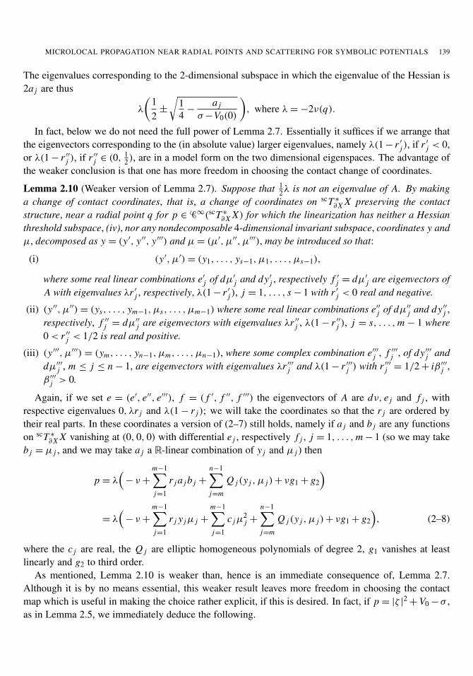
MICROLOCAL PROPAGATION NEAR RADIAL POINTS AND SCATTERING FOR SYMBOLIC POTENTIALS 139
The eigenvalues corresponding to the 2-dimensional subspace in which the eigenvalue of the Hessian is2a j are thus
λ
(12
±
√14
−a j
σ−V0(0)
), where λ= −2ν(q).
In fact, below we do not need the full power of Lemma 2.7. Essentially it suffices if we arrange thatthe eigenvectors corresponding to the (in absolute value) larger eigenvalues, namely λ(1 − r ′
j ), if r ′
j < 0,or λ(1 − r ′′
j ), if r ′′
j ∈ (0, 12), are in a model form on the two dimensional eigenspaces. The advantage of
the weaker conclusion is that one has more freedom in choosing the contact change of coordinates.
Lemma 2.10 (Weaker version of Lemma 2.7). Suppose that 12λ is not an eigenvalue of A. By making
a change of contact coordinates, that is, a change of coordinates on scT ∗
∂X X preserving the contactstructure, near a radial point q for p ∈ C∞(scT ∗
∂X X) for which the linearization has neither a Hessianthreshold subspace, (iv), nor any nondecomposable 4-dimensional invariant subspace, coordinates y andµ, decomposed as y = (y′, y′′, y′′′) and µ= (µ′, µ′′, µ′′′), may be introduced so that:
(i) (y′, µ′)= (y1, . . . , ys−1, µ1, . . . , µs−1),
where some real linear combinations e′
j of dµ′
j and dy′
j , respectively f ′
j = dµ′
j are eigenvectors ofA with eigenvalues λr ′
j , respectively, λ(1 − r ′
j ), j = 1, . . . , s − 1 with r ′
j < 0 real and negative.
(ii) (y′′, µ′′)= (ys, . . . , ym−1, µs, . . . , µm−1) where some real linear combinations e′′
j of dµ′′
j and dy′′
j ,respectively, f ′′
j = dµ′′
j are eigenvectors with eigenvalues λr ′′
j , λ(1 − r ′′
j ), j = s, . . . ,m − 1 where0< r ′′
j < 1/2 is real and positive.
(iii) (y′′′, µ′′′) = (ym, . . . , yn−1, µm, . . . , µn−1), where some complex combination e′′′
j , f ′′′
j , of dy′′′
j anddµ′′′
j , m ≤ j ≤ n − 1, are eigenvectors with eigenvalues λr ′′′
j and λ(1 − r ′′′
j ) with r ′′′
j = 1/2 + iβ ′′′
j ,β ′′′
j > 0.
Again, if we set e = (e′, e′′, e′′′), f = ( f ′, f ′′, f ′′′) the eigenvectors of A are dν, e j and f j , withrespective eigenvalues 0, λr j and λ(1 − r j ); we will take the coordinates so that the r j are ordered bytheir real parts. In these coordinates a version of (2–7) still holds, namely if a j and b j are any functionson scT ∗
∂X X vanishing at (0, 0, 0) with differential e j , respectively f j , j = 1, . . . ,m − 1 (so we may takeb j = µ j , and we may take a j a R-linear combination of y j and µ j ) then
p = λ(
− ν+
m−1∑j=1
r j a j b j +
n−1∑j=m
Q j (y j , µ j )+ νg1 + g2
)
= λ(
− ν+
m−1∑j=1
r j y jµ j +
m−1∑j=1
c jµ2j +
n−1∑j=m
Q j (y j , µ j )+ νg1 + g2
), (2–8)
where the c j are real, the Q j are elliptic homogeneous polynomials of degree 2, g1 vanishes at leastlinearly and g2 to third order.
As mentioned, Lemma 2.10 is weaker than, hence is an immediate consequence of, Lemma 2.7.Although it is by no means essential, this weaker result leaves more freedom in choosing the contactmap which is useful in making the choice rather explicit, if this is desired. In fact, if p = |ζ |2 + V0 −σ ,as in Lemma 2.5, we immediately deduce the following.

140 ANDREW HASSELL, RICHARD MELROSE AND ANDRÁS VASY
Lemma 2.11. For the function p = |ζ |2 + V0 −σ with V0 Morse, the contact map in Lemma 2.10 can betaken as the composition of the contact map on scT ∗
∂X X induced by a change of coordinates on X , withthe canonical relation of multiplication by a function of the form eiφ/x , φ ∈ C∞(X).
Remark 2.12. The canonical relation of multiplication by eiφ/x is given, in local coordinates (y, ν, µ),by the map
8φ : (y, ν, µ) 7→ (y, ν+φ(y), µ+ ∂yφ(y)),
that is, if we write 8φ(y, ν, µ)= (y, ν, µ), then µk = µk + ∂ykφ(y). Note that while φ is a function onX , the canonical relation only depends on φ|∂X , which is why we simply regard φ as a function on ∂Xand write φ(y) here.
Proof. As in the proof of Lemma 2.5 we may assume, by a change of coordinates on X , that thecritical point of V0 over which the radial point q lies is y = 0, that h − |µ|
2= O(|y|
2) and that theHessian of V0 at 0 is diagonal, so for each j , (dy j , dµ j ) is an invariant subspace of A. Note that in thecoordinates (y, ν, µ), q = (0, ν0, 0). With the notation of Remark 2.9 above, if dy j is an eigenvector ofthe Hessian with eigenvalue 2a j then the eigenvectors of A of eigenvalue λr j , respectively λ(1−r j ), aree j = (λ/2)(1 − r j )dy j + dµ j , respectively f j = (λ/2)r j dy j + dµ j ; see Remark 1.3 of [Hassell et al.2004]. In particular, if r j is real, so is f j .
Now, the contact map8φ induced by multiplication by eiφ/x as above acts on T ∗scT ∗
∂X X by pullbacks,namely
8∗
φ
( ∑k
y∗
k d yk + ν∗ d ν+
∑k
µ∗
k dµk
)=
∑k
y∗
k dyk + ν∗(dν+
∑j
(∂y jφ) dy j )+∑
k
µ∗
k(dµk +
∑j
∂y j ∂ykφ(y) dy j ).
Thus, by the above remark, 8 will map q to (0, 0, 0) provided φ(0) = −ν0, ∂y jφ(0) = 0 for all j . Inthis case, moreover, the pullback 8∗
φ will map dyk to dyk , dν to dν and dµk to dµk +∑
j ∂y j ∂ykφ(y).Correspondingly, by letting φ(y)= −ν0 +
∑m−1j=1 b j y2
j , b j = (λ/4)r j , (8−1φ )
∗ maps f j to dµ j , j =
1, . . . ,m −1. Since the Legendre vector field W ′ of (8−1φ )
∗ p is the pushforward of the Legendre vectorfield W of p under 8φ , it follows that dµ j is an eigenvector of the linearization of W ′ with eigenvalueλ(1 − r j ). As 8∗
φ also maps the 2-dimensional subspaces (dy j , dµ j ) (at (0, 0, 0)) to the 2-dimensionalsubspaces (dy j , dµ j ) (at q), and the latter are invariant under A, so are the former under the linearizationof W ′. This proves the lemma. �
3. Microlocal normal form
Let P ∈9∗,−1sc (X) be an operator with real principal symbol p obeying (2–2), as in the previous section,
and assume that q is a nondegenerate radial point for p. In this section we shall reduce p to a normalform, via conjugation with a scattering Fourier integral operator. We first pause to define such operators.
3.1. Scattering Fourier integral operators. Scattering Fourier integral operators (FIOs) are defined interms of conventional FIOs via the local Fourier transform, as defined in [Melrose and Zworski 1996].Let X be a manifold of dimension n with boundary, and (x, y) local coordinates where x is a boundarydefining function. We can always identify a neighbourhood U ⊂ ∂X of y0 ∈ ∂X with an open set
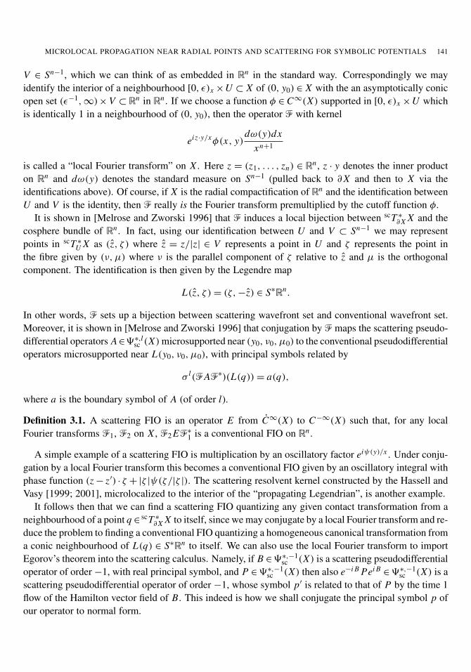
MICROLOCAL PROPAGATION NEAR RADIAL POINTS AND SCATTERING FOR SYMBOLIC POTENTIALS 141
V ∈ Sn−1, which we can think of as embedded in Rn in the standard way. Correspondingly we mayidentify the interior of a neighbourhood [0, ε)x ×U ⊂ X of (0, y0) ∈ X with the an asymptotically conicopen set (ε−1,∞)× V ⊂ Rn in Rn . If we choose a function φ ∈ C∞(X) supported in [0, ε)x ×U whichis identically 1 in a neighbourhood of (0, y0), then the operator F with kernel
ei z·y/xφ(x, y)dω(y)dx
xn+1
is called a “local Fourier transform” on X . Here z = (z1, . . . , zn) ∈ Rn , z · y denotes the inner producton Rn and dω(y) denotes the standard measure on Sn−1 (pulled back to ∂X and then to X via theidentifications above). Of course, if X is the radial compactification of Rn and the identification betweenU and V is the identity, then F really is the Fourier transform premultiplied by the cutoff function φ.
It is shown in [Melrose and Zworski 1996] that F induces a local bijection between scT ∗
∂X X and thecosphere bundle of Rn . In fact, using our identification between U and V ⊂ Sn−1 we may representpoints in scT ∗
U X as (z, ζ ) where z = z/|z| ∈ V represents a point in U and ζ represents the point inthe fibre given by (ν, µ) where ν is the parallel component of ζ relative to z and µ is the orthogonalcomponent. The identification is then given by the Legendre map
L(z, ζ )= (ζ,−z) ∈ S∗Rn.
In other words, F sets up a bijection between scattering wavefront set and conventional wavefront set.Moreover, it is shown in [Melrose and Zworski 1996] that conjugation by F maps the scattering pseudo-differential operators A∈9∗,l
sc (X)microsupported near (y0, ν0, µ0) to the conventional pseudodifferentialoperators microsupported near L(y0, ν0, µ0), with principal symbols related by
σ l(FAF∗)(L(q))= a(q),
where a is the boundary symbol of A (of order l).
Definition 3.1. A scattering FIO is an operator E from C∞(X) to C−∞(X) such that, for any localFourier transforms F1, F2 on X , F2 EF∗
1 is a conventional FIO on Rn .
A simple example of a scattering FIO is multiplication by an oscillatory factor eiψ(y)/x . Under conju-gation by a local Fourier transform this becomes a conventional FIO given by an oscillatory integral withphase function (z − z′) · ζ +|ζ |ψ(ζ/|ζ |). The scattering resolvent kernel constructed by the Hassell andVasy [1999; 2001], microlocalized to the interior of the “propagating Legendrian”, is another example.
It follows then that we can find a scattering FIO quantizing any given contact transformation from aneighbourhood of a point q ∈
scT ∗
∂X X to itself, since we may conjugate by a local Fourier transform and re-duce the problem to finding a conventional FIO quantizing a homogeneous canonical transformation froma conic neighbourhood of L(q) ∈ S∗Rn to itself. We can also use the local Fourier transform to importEgorov’s theorem into the scattering calculus. Namely, if B ∈9∗,−1
sc (X) is a scattering pseudodifferentialoperator of order −1, with real principal symbol, and P ∈9∗,−1
sc (X) then also e−i B Pei B∈9∗,−1
sc (X) is ascattering pseudodifferential operator of order −1, whose symbol p′ is related to that of P by the time 1flow of the Hamilton vector field of B. This indeed is how we shall conjugate the principal symbol p ofour operator to normal form.

142 ANDREW HASSELL, RICHARD MELROSE AND ANDRÁS VASY
3.2. Normal form. In this section we put the principal symbol of P into a normal form pnorm. For laterpurposes we shall also need the subprincipal symbol of P in a normal form, but only along the “flow-out”,that is, the unstable manifold, of q, which can be done via conjugation by a function; this is accomplishedin Lemma 6.1. (The model form of the subprincipal symbol only plays a role in the polyhomogeneous,as opposed to just conormal, analysis, which is the reason it is postponed to Section 6.)
For this purpose, we only need to construct the principal symbol σ(B) of B as in the first subsection.This in turn can be written as x−1b, b ∈ C∞(scT ∗X), so we only need to construct a function b on scT ∗
∂X Xsuch that the pullback 8∗ p of p by the time 1 flow 8 of Hx−1b is the desired model form pnorm, where bis some extension of b to scT ∗X; this property is independent of the chosen extension. Thus any B withσ(B)= b will conjugate P to an operator with principal symbol pnorm. This construction is accomplishedin two steps, following Guillemin and Schaeffer [1977] in the nonresonant setting. First we constructthe Taylor series of b at q = (0, 0, 0), which puts p into a model form modulo terms vanishing to infiniteorder at q . Next, we remove this error along the unstable manifold of q by modifying an argument dueto Nelson [1969].
Rather than using powers of I to filter the Taylor series of b, we proceed as in [Guillemin and Schaeffer1977] and assign degree 1 to y and µ but degree two to ν in local coordinates as discussed above. Thus,let h j denote the space of functions
h j=
∑2a+|α|+|β|−2= j
νa yαµβC∞(scT ∗
∂X X)
Note that this is well-defined, independently of our choice of local coordinates, since −dν is the contactform α at q , so ν is well-defined up to quadratic terms. The Poisson bracket preserves this filtration ofI in the following sense. If a, b are some smooth extensions to scT ∗X of elements a ∈ hi , b ∈ h j then
x−1c = {x−1a, x−1b} H⇒ c = c|scT ∗
∂X X ∈ hi+ j .
When this holds we write c = {{a, b}}; explicitly,
{{a, b}} = Wa(b)+∂a∂ν
b −∂b∂ν
a, (3–1)
with W given by (2–4). Thus
{{., .}} : hi× h j
7→ hi+ j .
We then consider the quotient
g j= h j/h j+1,
so the bracket {{., .}} descends to
gi× g j
→ gi+ j .
Remark 3.2. These statements remain true with h j replaced by I j . However, note that p = −ν in I/I2,since dp = −dν at q, but it is not the case that p = −ν in g0. In fact, p is given by (3–2) below in g0.
Using contact coordinates as discussed above, g j may be freely identified with the space of homoge-neous functions of ν, y, µ of degree j + 2 where the degree of ν is 2. Now let p0 be the part of p of

MICROLOCAL PROPAGATION NEAR RADIAL POINTS AND SCATTERING FOR SYMBOLIC POTENTIALS 143
homogeneity degree two. In order to use Lemmas 2.7 and 2.10, we assume throughout the paper fromhere on that case (iv) above Lemma 2.7 does not apply. Hence from (2–7)
p0 = λ(
− ν+
m−1∑j=1
r j y jµ j +
n−1∑j=m
Q j (y j , µ j )), p − p0 ∈ h1. (3–2)
If we take b ∈ hl , l ≥ 1 and let 8 be the time 1 flow of Hx−1b then
x8∗(x−1 p)= p + {{p, b}} = p + {{p0, b}}, modulo hl+1.
This allows us to remove higher order term in the Taylor series of the symbol successively provided wecan solve the “homological equation”
{{p0, b}} = e ∈ hl, modulo hl+1.
Thus we need to consider the range of this linear map; its eigenfunctions are easily found from theeigenfunctions of the linearization of W .
Lemma 3.3. The (equivalence classes of the) monomials pa0 eα f β with 2a + |α| + |β| = l + 2 satisfy
{{p0, pa0 eα f β}} = Ra,α,β pa
0 eα f β
with eigenvalues
Ra,α,β = λ(
a − 1 +
n−1∑j=1
α jr j +
n−1∑j=1
β j (1 − r j ))
(3–3)
and give a basis of eigenvectors for {{p0, .}} acting on gl .Here we identify the differentials e j and f j with linear functions with these differentials.
Remark 3.4. In fact, the contact coordinates given by Lemma 2.10 suffice for the proof of this lemma;the additional information in Lemma 2.7 is not needed. In this case, by (2–8),
p0 = λ(
− ν+
m−1∑j=1
r j e j f j +
n−1∑j=m
Q j (y j , µ j )).
We also remark that we could equally well use the eigenvector basis for {{p0, .}} acting on gl given byνaeα f β with 2a + |α| + |β| = l + 2. This follows from the lemma using that
ν =
m−1∑j=1
r j y jµ j +
n−1∑j=m
Q j (y j , µ j )− λ−1 p0
in g0, and y jµ j as well as Q j (y j , µ j ) are eigenvectors with eigenvalue λ(r j +(1−r j ))= λ, and so is p0.
Proof. Taking into account the eigenvalues and eigenvectors of A, all eigenvalues and eigenvectors of{{p0, .}} can be calculated iteratively using the derivation property of the original Poisson bracket. This

144 ANDREW HASSELL, RICHARD MELROSE AND ANDRÁS VASY
implies
{{p0, ab}} = x{x−1 p0, x(x−1a)(x−1b)}
= x−1{x−1 p0, x}ab + x{x−1 p0, x−1a}b + xa{x−1 p0, x−1b}
= λab + {{p0, a}}b + a{{p0, b}},
where each term within {., .} really uses a C∞ extensions of the a, b, p0 to scT ∗X , followed by evaluationof the bracket and then restriction to scT ∗
∂X X . Since
{{p0, a}} = x{x−1 p0, x−1a} = x{x−1 p0, x−1}a + {x−1 p0, a} = −λa + {x−1 p0, a},
on g−1 the eigenvectors of {{p0, .}} are the eigenvectors e j and f j of A with eigenvalues −λ+ λr j and−λ+λ(1−r j ). Moreover, in g0, p0 is an eigenvector of {{p0, .}} with eigenvalue 0. Thus, e j , f j and p0
satisfy the claim of the lemma. Since the other generators of g0, as well as generators of g j , j ≥ 1, canbe written as a products of the e j , f j and p0, the conclusion of the lemma follows by induction. �
Definition 3.5. We call the multiindices in the set
I ={(a, α, β); Ra,α,β = 0 and 2a + |α| + |β| ≥ 3
}, (3–4)
with Ra,α,β given by (3–3), resonant.
Conjugation therefore allows us to remove, by iteration, all terms except those with indices in I .Expanding pa
0 using (3–2) we deduce the following.
Proposition 3.6. If P is as above and the leading term of p = σ∂,−1(P) is given by (3–2) near a givenradial point q then there exists a local contact diffeomorphism 8 near q such that
8∗ p =λ(
− ν+
m∑j=1
r j y jµ j +
n−1∑j=m+1
Q j (y j , µ j )+∑
(a,α,β)∈I
ca,α,βνaeα f β
)modulo I∞
= h∞ at q (3–5)
with I given by (3–4).
Proof. The Taylor series of8 at q can be constructed inductively over the filtration h j as indicated above.At the j–th stage, the terms of weighted homogeneity j can be removed from p except for those in thenull space of {{p0, ·}}, that is, the resonant terms with Ra,α,β = 0. This leads to (3–5) in the sense offormal power series. However, by use of Borel’s Lemma a local contact diffeomorphism can be foundgiving (3–5). �
Now a small extension of Nelson’s proof of Sternberg’s linearization theorem can be used to removethe infinite order vanishing error along the unstable manifold, that is, at ν = 0, µ= 0, y′′
= 0, y′′′= 0.
Proposition 3.7. Suppose that X and X0 are C∞ vector fields on RN with X0(0)= 0 and X1 = X − X0
vanishing to infinite order at 0. Suppose also that they are both linear outside a compact set and equalthere to their common linearization, DX (0), at 0 which is assumed to have no pure imaginary eigenvalue.Let U (t), U0(t) be the flows generated by X and X0. If E is a linear submanifold invariant under X0
such thatlim
t→∞U0(t)x = 0 for all x ∈ E (3–6)

MICROLOCAL PROPAGATION NEAR RADIAL POINTS AND SCATTERING FOR SYMBOLIC POTENTIALS 145
then for all j = 0, 1, 2, . . . and x ∈ E
limt→∞
D j (U (−t)U0(t))x (3–7)
exists, and is continuous in x ∈ E , and
W−x = limt→∞
U (−t)U0(t)x, x ∈ E
has a C∞ extension, G, to RN which is the identity to infinite order at 0 and such that (G−1)∗X = X0 toinfinite order along E in a neighbourhood of 0.
Remark 3.8. Note that the derivatives D j in (3–7) refer to the ambient space RN , and not merely to E .This is useful in producing the Taylor series of G for the last part of the conclusion.
Also, the limit t → ∞ means t → +∞, as in Nelson’s book.
Proof. We follow the proof of Theorem 8 in [Nelson 1969]. Indeed, if X0 was assumed to be linearthen Nelson’s theorem would apply directly. Dropping this assumption has little effect on the proof; themain difference is that a little more work is required to show the exponential contraction property, (3–8)below.
Since the real part of every eigenvalue of DX (0) is nonzero, RN= E+ ⊕ E− where E+, respectively
E−, is the direct sum of the generalized eigenspaces of DX (0) with eigenvalues with positive, respec-tively negative, real parts. Since E is invariant under X0, and hence under DX (0), necessarily E ⊂ E−.We actually apply the theorem with E = E−, but, as in Nelson’s discussion, the more general case isuseful for the inductive argument for the derivatives.
Let e j denote a basis of E− consisting of generalized eigenvectors of DX (0) with correspondingeigenvalue σ j ; we shall consider the e j as differentials of linear functions f j on RN . For x ∈ RN , letx(t)= U0(t)x , F j (t)= f j (x(t)). Then d F j/dt |t=t0 = (X0 f j )(x(t0)) where
X0 f j (y)= DX (0) f j (y)+ O(‖y‖2).
Moreover, for y ∈ E−, ‖y‖2≤ C1
∑j f 2
j for some C1 > 0. So, setting ρ =∑
f 2j , we deduce that
X0ρ(y)=
∑j
2σ j f 2j (y)+ O(ρ(y)3/2),
hence with R(t)= ρ(x(t)), c0 ∈ (sup σ j , 0), there exists δ > 0 such that for ‖R(t)‖ ≤ δ,
d Rdt
− 2c0 R ≤ 0,
and hence R(t)≤ e−2c0t‖x‖ for t ≥ 0, ‖r(x)‖ ≤ δ, x ∈ E−. A corresponding estimate also holds outside
a compact set, as X0 is given by DX (0) there, so a patching argument and (3–6) yield the estimateR(t)≤ C0e−2c0t
‖x‖ for all x ∈ E−. Since R(t)1/2 is equivalent to ‖.‖, we deduce that there are constantsC , c > 0 such that
‖U0(t)x‖ ≤ Ce−ct‖x‖ ∀ x ∈ E and t ≥ 0. (3–8)
For the remainder of the argument we can follow Nelson’s proof even more closely. Thus, let κ be aLipschitz constant for X and X0, and choose m such that cm > κ . Note that there exists c0 > 0 such that

146 ANDREW HASSELL, RICHARD MELROSE AND ANDRÁS VASY
for all x ∈ RN ,‖X1(x)‖ ≤ c0‖x‖
m, X1 = X − X0. (3–9)
For t1 ≥ t2 ≥ 0, t1 = t2 + t , x ∈ E ,
I = ‖U (−t1)U0(t1)x − U (−t2)U0(t2)x‖ = ‖U (−t2) (U (−t)U0(t)− Id)U0(t2)x‖
≤ eκt2‖(U (−t)U0(t)− Id)U0(t2)x‖
by the Lipschitz condition (see [Nelson 1969, Theorem 5]). But with X = X0 + X1, by [Nelson 1969,Proof of Theorem 6, (5)]
‖U (−t)U0(t)y − y‖ ≤
∫ t
0eκs
‖X1(U0(s)y)‖ ds.
Applying this with y = U0(t2)x , we deduce that
I ≤ eκt2∫ t
0eκs
‖X1(U0(s + t2)x)‖ ds. (3–10)
Thus, by (3–9) and (3–8),
I ≤ eκt2∫ t
0eκsc0Cme−cm(s+t2)‖x‖
m ds ≤ eκt2∫
∞
0eκsc0Cme−cm(s+t2)‖x‖
m ds =c0Cme−(cm−κ)t2‖x‖
m
cm − κ.
Letting t2 → ∞ shows that W−x = limt→∞ U (−t)U0(t)x exists, with convergence uniform on compactsets, hence W− is continuous in x ∈ E . Moreover, applying the estimate with t2 = 0 shows that W−(x)−x = O(‖x‖
m). Since m is arbitrary, as long as it is sufficiently large, this shows that W− is the identity toinfinite order at 0, provided it is smooth, as we proceed to show.
Smoothness can be seen by a similar argument, although we need to put a slight twist into Nelson’sargument. Namely, first consider the first derivatives, or rather the 1-jet. Thus, we work on RN
⊕L(RN ).Let (x, ξ) denote the components with respect to this decomposition. These evolve under the flow U ′(t),respectively U ′
0(t), given by
X ′(x, ξ)= (X (x), DX (x) · ξ), X ′
0(x, ξ)= (X0(x), DX0(x) · ξ),
where DX (x) and ξ are considered as elements of L(RN ), and · is composition of operators. Note thatthe second, L(RN ), component of these vector fields is a homogeneous degree zero vector field, that is,it is invariant under pushforward by the natural R+-action (by dilations).
The twist, as compared to Nelson’s work, is that we identify L(RN ) with RN 2, which we radially
compactify to a (closed) ball B N 2, which we further embed as the closed unit ball in RN 2
in such afashion that the smooth structure of the ball agrees with the restriction of the smooth structure fromRN 2
. Let ι : RN 2→ RN 2
be this map with range the interior of B N 2. Then the pushforward under ι of a
homogeneous degree zero vector field, such as DX (x)·ξ is for each x ∈ RN , extends to a C∞ vector fieldon the closed ball B N 2
, which by homogeneity is tangent to the boundary. Furthermore, if ι1 = idRN × ι,then (ι1)∗X ′ and (ι1)∗X ′
0 extend to C∞ vector field on RN× B N 2
tangent to the boundary and theirdifference, (ι1)∗X ′
1, in addition vanishes to infinite order at {0} × B N 2. Thus (ι1)∗X ′ and (ι1)∗X ′
0 areLipschitz with some Lipschitz constant κ ′: this is automatic over a compact subset of RN
× B N 2, which

MICROLOCAL PROPAGATION NEAR RADIAL POINTS AND SCATTERING FOR SYMBOLIC POTENTIALS 147
in fact suffices here, but in fact holds on all of RN× B N 2
since outside the inverse image of a compactsubset of RN
× B N 2, X ′ and X ′
0 are linear, so in particular their B N 2component is independent of x .
To minimize confusion about the “change of coordinates”, we write the coordinates on RN× B N 2
as (x, η) below. With c as in (3–8), choose m such that cm > κ ′. Then the infinite order vanishing of(ι1)∗X ′
1 at x = 0 yields‖((ι1)∗X ′
1)(x, η)‖ ≤ c′
0‖x‖m
for all (x, η). Let U ′(t), U ′
0(t) denote the evolution groups generated by (ι1)∗X ′ and (ι1)∗X ′
0, respectively.Thus, for all real t ,
‖U ′(t)(x, η)‖ ≤ eκ′t‖(x, η)‖, (3–11)
see [Nelson 1969, Theorem 5]. So (3–10) still applies, with X1 replaced by (ι1)∗X ′
1, κ replaced by κ ′,etc. Thus, by (3–8) and (3–11),
I ′= ‖U ′(−t1)U ′
0(t1)(x, η)− U ′(−t2)U ′
0(t2)(x, η)‖
≤ eκ′t2
∫ t
0eκ
′s‖((ι1)∗X ′
1)(U′
0(s + t2)(x, η))‖ ds
≤ eκ′t2
∫ t
0eκ
′sc′
0Cme−cm(s+t2)‖x‖m ds
≤ eκ′t2
∫∞
0eκ
′sc′
0Cme−cm(s+t2)‖x‖m ds =
c′
0Cme−(cm−κ ′)t2‖x‖m
cm − κ ′.
Thus, limt→∞ U ′(−t)U ′
0(t)x exists, with convergence uniform on compact sets, so the limit dependscontinuously on (x, ξ) for x ∈ E .
The higher derivatives can be handled similarly. The resulting Taylor series about E can be summedasymptotically, giving G: this part of the argument of Nelson is unchanged. �
3.3. Effective resonance and nonresonance. Next we apply this general result to the symbol p. Fol-lowing Lemma 2.7, when resonances occur we cannot remove all error terms even in the sense of formalpower series. Consequently we do not attempt to get a full normal form in a neighbourhood of the criticalpoint, but only along the submanifold
S = {ν = 0, y′′= 0, y′′′
= 0, µ= 0}, (3–12)
which is the unstable manifold for W0. After reduction to normal form, errors which are polynomial inthe normal directions to S will remain. For later purposes, we divide these into two parts.
Definition 3.9. With I as in Definition 3.5, let
Ier = I ′
er ∪ I ′′
er,
I ′
er = {(a,α,β)∈ I : α= (α′,α′′,α′′′), β = (β ′,β ′′,β ′′′),a = 0, α′′′= 0, β ′′′
= 0, α′′= 0, β ′′
= 0, |β ′| = 1},
I ′′
er = {(a,α,β)∈ I : α= (α′,α′′,α′′′), β = (β ′,β ′′,β ′′′), a = 0, α′′′= 0, β ′′′
= 0, α′= 0, β ′
= 0}. (3–13)
An effectively resonant function is a polynomial of the form
rer =∑
(a,α,β)∈Ier
ca,α,β pa0 eα f β,

148 ANDREW HASSELL, RICHARD MELROSE AND ANDRÁS VASY
or equivalentlyrer =
∑(a,α,β)∈Ier
ca,α,β νaeα f β .
Thus, elements of Ier satisfy (0, α, β)∈ I (that is, are resonant; see Definition 3.5), with α= (α′, α′′, 0),β = (β ′, β ′′, 0), and either α′′
= 0, β ′′= 0, |β ′
| = 1, or α′= 0, β ′
= 0.Moreover, an effectively resonant function has the form∑
α′,|β ′|=1
cα′β ′(e′)α′
( f ′)β′
+
∑α′′,β ′′
cα′′β ′′(e′′)α′′
( f ′′)β′′
. (3–14)
For a fixed critical point of a fixed operator P (for example, P = x−1(1+ V − σ) for a fixed σ ),the set Ier is finite. Thus, only a finite number of terms can occur in (3–14), and hence restricting topolynomials in the definition of effectively resonant functions (rather than infinite formal sums) is in factnot a restriction. To see this, note that in the expression for Ra,α,β in (3–4), we have a = 0, α′′′
= β ′′′= 0
and either (i) α′′= β ′′
= 0 and |β ′| = 1 or (ii) α′
= β ′= 0. In case (i), if β ′
j = 1 then to haveRa,α,β = 0 we need
∑α′
kr ′
k = r ′
j , which is only possible for |α′| ≤ |r ′
j |/mink |r ′
k |. In case (ii), we need∑α′′
j r′′
j +∑β ′′
j (1−r ′′
j )= 1, which is only possible for |α′′| ≤ 1/min r ′′
k and |β ′′| ≤ 2. (Actually in case
(ii) we must have |β ′′| ≤ 1 in order to satisfy the condition 2a + |α| + |β| ≥ 3 in (3–4).)
Definition 3.10. Let JS denote the ideal of C∞ functions on scT ∗
∂X X which vanish on S and set
J ′′=
{(α′′, β ′′);
m−1∑j=s
r ′′
j α′′
j + (1 − r ′′
j )β′′
j ∈ (1, 2)}.
An effectively nonresonant function is an element of JS of the form
renr =
s−1∑j=1
h j f ′
j +
∑(α′′,β ′′)∈I ′′
h′′
α′′,β ′′eα′′
f β′′
+
∑j,k
h′′′
jke′′′
j f ′′′
k
h j ∈ JS, j = 0, 1, . . . , s, h′′
α′′,β ′′ ∈ C∞(scT ∗
∂X X), (α′′, β ′′) ∈ I ′′,
h′′′
jk ∈ JS, j, k = m, . . . , n − 1. (3–15)
Note that J ′′ is finite, hence all sums in the definition are finite.
Theorem 3.11. Using the notation of Lemma 2.7 for coordinates near a radial point of q of p there isa local contact diffeomorphism 8 from a neighbourhood of (0, 0, . . . , 0) to a neighbourhood of q suchthat 8∗ p = pnorm such that
λ−1 pnorm = −ν+
∑j
r j y jµ j +
n−1∑j=m
Q j (y j , µ j )+ renr + rer, (3–16)
with renr of the form (3–15) and rer of the form (3–14); in addition at a nonresonant critical point, thatis, if I = ∅, then we may take renr = rer = 0 near q.
Remark 3.12. If F is an elliptic Fourier integral operator with canonical relation 8 then P = F−1 P Fsatisfies σ∂,−1(P)= pnorm.
MICROLOCAL PROPAGATION NEAR RADIAL POINTS AND SCATTERING FOR SYMBOLIC POTENTIALS 149
Remark 3.13. As will be seen below, of the two error terms, only rer has any effect on the leadingasymptotics of microlocal solutions. The construction below shows that modulo I∞, renr may be chosento consist of resonant terms only, that is, to be an asymptotic sum of resonant terms. However, this playsno role in the paper; all the relevant information is contained in the statement of the theorem.
Remark 3.14. We do not need the full power of Lemma 2.7 to find 8 as in this theorem; Lemma 2.10suffices. Indeed, the terms
∑m−1j=1 c jµ
2j in (2–8) can be absorbed in renr.
Similarly any term νaµβ yα with a +|β| ≥ 2 and a 6= 0, or with |β| ≥ 3 can be included in rer or renr.The same is true for any term with |β| ≥ 2 such that β j 6= 0 for some j with Re r j 6=
12 . In particular, if
Re r j 6=12 for any j , the only terms which need to be removed have a +|β| ≤ 1. The conjugating Fourier
integral operator can therefore also be arranged to have such terms only and thus to be of the form ei B ,with B = Z +( f/x) where Z is a vector field on X tangent to its boundary and f is a real valued smoothfunction on X . Correspondingly, the normal form may be achieved by conjugation of P by an oscillatoryfunction, ei f/x , followed by pullback by a local diffeomorphism of X , that is, a change of coordinates.However, if Re r j =
12 for some j , some quadratic terms in µ would also need to be removed for the
model form, but since they play a role analogous to rer, the arguments of Section 5, giving conormality,are unaffected, and only the polyhomogeneous statements of Section 6 would need alterations. However,the contact diffeomorphism (that is, FIO conjugation) approach we present here is both more unified andmore concise.
If p = |ζ |2 + V0 − σ , the model form of Lemma 2.10 also only required a change of coordinatesand multiplication by an oscillatory function (see Lemma 2.11), the model form of this theorem can beobtained by these two operations, starting from the original operator P with symbol p.
Proof. First we apply Proposition 3.6. Next we need to show that rer as in (3–14) and renr as in (3–14)can be chosen to have Taylor series at 0 given exactly by the error term in (3–5).
So, consider a monomial νaeα f β with (a, α, β) ∈ I . If α′′′6= 0 then β ′′′
6= 0 since Im r ′′′
j > 0, andonly the eigenvalues of f ′′′
j have negative imaginary parts, and conversely. In addition, 2a +|α|+ |β| ≥
3 implies that a monomial with α′′′6= 0 or β ′′′
6= 0 has the form νaeα f βe′′′
j f ′′′
k for some j, k with2a + |α| + |β| ≥ 1 and
Re(a +
∑rl αl +
∑(1 − rl)βl)= 0.
Since Re(1−rl) > 0 for all l and Re rl > 0 for l ≥ s, while rl < 0 for l ≤ s −1, we must have α′6= 0 (that
is, αl 6= 0 for some l ≤ s − 1) and correspondingly a + |α′′| + |α′′′
| + |β|> 0. Due to the latter, νaeα f β
vanishes on S, so the terms with α′′′6= 0 or β ′′′
6= 0 appear in renr.So we may assume that α′′′
= β ′′′= 0. If a 6= 0, the monomial is of the form ν aeα f βν, a = a − 1,
2a + |α| + |β| ≥ 1 with
a +
∑r j α j +
∑(1 − r j )β j = 0.
Arguing as in the previous paragraph we deduce that the terms with a 6= 0 also appear in renr.So we may now assume that a = 0, α′′′
= β ′′′= 0. If β ′
6= 0, the monomial is of the form νaeα f β f j
for some j , and 2a + |α| + |β| ≥ 2,
a +
∑rl αl +
∑(1 − rl)βl = r j < 0.

150 ANDREW HASSELL, RICHARD MELROSE AND ANDRÁS VASY
We can still conclude that α′6=0, but it is not automatic that a+|α′′
|+|β|>0. However, if a+|α′′|+|β|>0
then νaeα f β f j is again included in renr, while if a +|α′′|+|β| = 0, then the monomial is included in rer.
Finally then, we may assume that a = 0, β ′= 0, α′′′
= β ′′′= 0. Since r ′
j < 0 for all j = 1, . . . , s − 1∑(r ′′
j α′′
j + (1 − r ′′
j )β′′
j )≥
∑r ′
jα′
j +
∑(r ′′
j α′′
j + (1 − r ′′
j )β′′
j )= 1.
Moreover, the equality holds if and only if α′= 0, in which case this term is included in rer. The terms
with α′6= 0 can be included in h′′
α′′,β ′′eα
′′
f β′′
for some α′′≤ α′′, β ′′
≤ β ′′, chosen by reducing α′′ and/orβ ′′ to make ∑
(r ′′
j α′′
j + (1 − r ′′
j )β′′
j ) ∈ (1, 2).
This can be done since r ′′
j , 1 − r ′′
j ∈ (0, 1).It follows that λ−1 p can be conjugated to the form
−ν+
∑j
r j y jµ j +
n−1∑j=m
Q j (y j , µ j )+ renr + rer + r∞, (3–17)
where renr, rer are as in (3–15), (3–14), with both vanishing if q is nonresonant, and r∞ vanishes toinfinite order at (0, 0, 0). Thus, it remains to show that we can remove the r∞ term in a neighbourhoodof the origin.
To do this we apply Proposition 3.7. Let X ′ be the Legendre vector field of (3–17), and let X ′
1 bethe Legendre vector field of r∞, while X ′
0 = X ′− X ′
1. Let X be the linear vector field with differentialequal to DX (0), let χ be compactly supported, identically 1 near 0, and let X = −(χX ′
+ (1 − χ)X),X0 = −(χX ′
0 +(1−χ)X). The overall minus sign is due to S being the unstable manifold of X ′
0 near theorigin, hence the stable manifold of −X ′
0. Let E be the subspace S of R2n−1, defined by (3–12). ThenProposition 3.7 is applicable, and G given by it may be chosen as a contact diffeomorphism since U (t),U0(t) are such; see [Guillemin and Schaeffer 1977, Section 3, Theorem 4]. �
3.4. Parameter-dependent normal form. We also need a parameter-dependent version of this theorem.Namely, suppose that p depends smoothly on a parameter σ , can we make the normal form dependsmoothly on σ as well? This problem can be approached in at least two different ways. One canconsider σ simply as a parameter, so p ∈ C∞((∂scT ∗X)× I )= C∞((scT ∗
∂X X)× I ) and then try to carryout the reduction to normal form uniformly. Alternatively, one identify p with the function p′ on thelarger space ∂scT ∗(X × I ) arising by the pullback under the natural projection
p′= π∗ p, π :
scT ∗
∂X×I (X × I )→ (scT ∗
∂X X)× I
and then carry out the reduction to a model on the larger space. Whilst the second approach may be morenatural from a geometric stance, we will adopt the first, since it is closer to the point of view of spectraltheory of [Hassell et al. 2004]. Clearly the difficulty in obtaining a uniform normal form is particularlyacute near a value of σ at which the effectively resonant terms do not vanish. Fortunately in the case ofcentral interest here, and in other cases too, the set of points at which such problems arise is discrete.
Lemma 3.15. If P = P(σ ) = x−1(1+ V − σ), q = q(σ ) is a radial point of P lying over the criticalpoint z = π(q) of V0 and I (σ ), respectively Ier(σ ), are the sets (3–4), respectively (3–13), for p(σ ) then

MICROLOCAL PROPAGATION NEAR RADIAL POINTS AND SCATTERING FOR SYMBOLIC POTENTIALS 151
the set Rz = RHt,z ∪ Rer,z , defined by
RHt,z ={σ ∈ (V0(z),+∞) | ∃ j such that r j =
12
},
Rer,z ={σ ∈ (V0(z),+∞) | Ier(σ ) 6= ∅
},
that is, the set of energies σ which are either a Hessian threshold (see Lemma 2.7) or such that q(σ ) hasa nontrivial effectively resonant error term (see Definition 3.9), is discrete in (V0(π(q)),+∞).
Remark 3.16. It follows that if K ⊂ (V0(z),+∞) is compact then K ∩ Rz is finite. Thus, to proveproperties such as asymptotic completeness, one can ignore all σ ∈ K which are Hessian thresholds oreffectively resonant.
Note also that by the definition of Ier(σ ),
Rer,z ={σ ∈ (V0(z),+∞) | either ∃ (0, (α′, 0, 0), (β ′, 0, 0)) ∈ I (σ ) with |β ′
| = 1
or ∃ (0, (0, α′′, 0), (0, β ′′, 0)) ∈ I (σ )}.
Proof. Using Remark 2.9, the set RHt,z of Hessian thresholds is given by {V0(z) + 4a j } where a j isan eigenvalue of the Hessian of V0 at z and hence has cardinality at most n − 1, so this set is triviallydiscrete.
Let K be a compact subset of (V0(z),+∞). The set K ∩Rer,z of effectively resonant energies in K isthe union of zeros of a finite number of analytic functions (none of which are identically zero). Indeed,Rer,z is given by the union of the set of zeros of the countable collection of functions
−1 +
m−1∑j=s
α′′
j r′′
j (σ )+β′′
j (1 − r ′′
j (σ )), −1 + (1 − rk)+
s−1∑j=1
α′
jr′
j (σ )
as k = 1, . . . , s −1, while α′, α′′, β ′′ are multiindices. But if c> 0 is large enough then c−1> |r j (σ )|> cfor all j and for all σ ∈ K as K is compact and the r j do not vanish there. Correspondingly, for |α′
|>2/c2,
−1 + (1 − rk)+
s−1∑j=1
α′
jr′
j (σ ) <−rk − |α′|c <−c−1,
and analogously for |α′′| + |β ′′
|> 2/c,
−1 +
m−1∑j=s
α′′
j r′′
j (σ )+β′′
j (1 − r ′′
j (σ )) >−1 + (|α′′| + |β ′′
|)c > 1.
Thus, there are only a finite number of these analytic functions that may vanish in K , as claimed. �
If q(σ ) are the radial points corresponding to z ∈ Cv(V ), and σ /∈ Rer,z , then we will say that q(σ ) iseffectively nonresonant, or that σ is an effectively nonresonant energy for z. We now prove that, awayfrom effectively resonant energies and Hessian thresholds, we have a normal form for p(σ ) of the form(3–16) with rer = 0 and depending smoothly on σ . Thus, for a given critical point z of V0, consider anopen interval O ⊂ (V0(z),+∞)\Rz . Apart from the coefficients h j , h′′
α′′,β ′′ , etc., in (3–15) the only part
152 ANDREW HASSELL, RICHARD MELROSE AND ANDRÁS VASY
of the model form depending on σ is
J ′′(σ )=
{(α′′, β ′′);
m−1∑j=s
r ′′
j (σ )α′′
j + (1 − r ′′
j (σ ))β′′
j ∈ (1, 2)}.
We note that on compact subsets K of O , there is a c > 0 such that r ′′
j (σ ) > c for σ ∈ K , and then for|α′′
| + |β ′′|> 2c−1,
sα′′β ′′(σ )=
m−1∑j=s
r ′′
j (σ )α′′
j + (1 − r ′′
j (σ ))β′′
j > 2,
so if we letJK =
⋃σ∈K
J ′′(σ ),
then JK is a finite set of multiindices. For each multiindex (α′′, β ′′) we let
Oα′′,β ′′ = s−1α′′β ′′((1, 2)), (3–18)
which is thus an open subset of O .For the parameter dependent version of the Theorem 3.11 we introduce
S = {(y, ν, µ, σ ); ν = 0, y′′= 0, y′′′
= 0, µ= 0, σ ∈ O},
in place of S (3–12).
Theorem 3.17. Suppose that p ∈ C∞(scT ∗
∂X X × O), O ⊂ (V0(z),+∞) \ Rz is open, that the symplecticmap S induced by the linearization A′ of p at q(σ ) (see Lemma 2.3) can be smoothly decomposed(as a function of σ ∈ O) into two-dimensional invariant symplectic subspaces and that there existsc > 0 such that r ′′
j (σ ) > c for σ ∈ O. Then 8(σ) and F(σ ) can be chosen smoothly in σ so thatpnorm(σ )= σ1(P(σ )), P(σ ) = F(σ )−1 P(σ )F(σ ), is of the form in Theorem 3.11, with rer ≡ 0, withthe sum over J ′′ replaced by a locally finite sum (the sum is over JK over compact subsets K ⊂ O), theh j , etc., in (3–15) depending smoothly on σ , that is, they are in C∞(scT ∗
∂X X × O), vanishing at S as inTheorem 3.11, and with the h′′
α′′β ′′ supported in scT ∗
∂X X × Oα′′β ′′ in terms of (3–18).
Remark 3.18. For P = x−1(1+ V − σ) the conditions of the theorem are satisfied for any boundedO = I disjoint from the discrete set of effectively resonant σ , since in local coordinates (y, µ) on 6(σ),the eigenspaces of S are independent of σ as shown in the proof of Lemma 2.5, and the r ′′
j are boundedbelow by Remark 2.9.
Proof. Since the invariant subspaces depend smoothly on σ by assumption, so do the eigenvalues of thelinearization, and there is smooth family of local contact diffeomorphisms, that is, coordinate changes,under which p(σ ) takes the form (2–7), that is,
p(σ )= λ(σ)(
− ν+
m−1∑j=1
r j (σ )y jµ j +
n−1∑j=m
Q j (σ, y j , µ j )+ νg1 + g2
)the Q j (σ, .), are homogeneous polynomials of degree 2, g1 vanishes at least linearly and g2 to thirdorder, all depending smoothly on σ .

MICROLOCAL PROPAGATION NEAR RADIAL POINTS AND SCATTERING FOR SYMBOLIC POTENTIALS 153
For the rest of the argument it is convenient to reduce the size of the parameter set O as follows. Forσ ∈ O , let
O(σ )=
( ⋂(α′′,β ′′):
sα′′,β′′ (σ )∈(1,2)
s−1α′′,β ′′((1, 2))
)∩
( ⋂(α′′,β ′′):
sα′′,β′′ (σ )∈(−∞,1)
s−1α′′,β ′′((−∞, 1))
), (3–19)
an open set (as it is a finite intersection of open sets) that includes σ . Thus, {O(σ ) : σ ∈ O} is an opencover of O . Take a locally finite subcover and a partition of unity subordinate to it. It suffices now toshow the theorem for each element O(σ0) of the subcover in place of O , for we can then paste togetherthe models pnorm we thus obtain using the partition of unity. Thus, we may assume that O = O(σ0) forsome σ0 ∈ O , and prove the theorem with the sum over J ′′ replaced by a sum over J ′′(σ0). Hence, onO , for any (α′′, β ′′) either
(a) sα′′β ′′(σ0) > 1, and then for some (α′′, β ′′) ∈ J ′′(σ0), (α′′, β ′′) ≥ (α′′, β ′′) (reduce |α′′| + |β ′′
| untilsα′′,β ′′ ∈ (1, 2) – this will happen as r j ∈ (0, 1/2)) hence sα′′β ′′(σ ) ≥ sα′′β ′′(σ ) > 1 for all σ ∈ O bythe definition of O(σ0), or
(b) sα′′β ′′(σ0) < 1, and then sα′′β ′′(σ ) < 1 for all σ ∈ O by the definition of O(σ0).
In order to make 8(σ) smooth in σ , we slightly modify the construction of the local contact diffeo-morphism 81(σ ) in Proposition 3.6 so that for any given σ we do not necessarily remove every term wecan (that is, which are nonresonant for that particular σ ). Namely, we choose the set I ′ of multiindices(a, α, β) which we do not remove by 81(σ ) so that I ′ is independent of σ , and such that I ′ containsevery multiindex which is resonant for some σ ∈ O , that is, I ′
⊃⋃σ∈O I (σ ), with I (σ ) denoting the set
of multiindices corresponding to resonant terms for p(σ ), as in Proposition 3.6. With any such choice ofI ′, the local contact diffeomorphism of Proposition 3.6, 81(σ ), can be chosen smoothly in σ such thatλ−18∗
1 p is of the form
−ν+
m∑j=1
r j (σ )y jµ j +
n−1∑j=m+1
Q j (σ, y j , µ j )+∑
I ′
caαβ(σ )νaeα f β modulo I∞
= h∞ at q,
with caαβ depending smoothly on σ .The requirement I ′
⊃⋃σ∈O I (σ ) means that for (a, α, β) 6∈ I ′, Ra,α,β(σ ) must not vanish for σ ∈ O .
Here we recall that Ra,α,β(σ ) is the eigenvalue of {{p0, .}} defined by (3–3), namely
Ra,α,β(σ )= λ(
a − 1 +
n−1∑j=1
α jr j (σ )+
n−1∑j=1
β j (1 − r j (σ ))). (3–20)
Keeping this in mind, we choose I ′ by defining its complement (I ′)c to consist of multiindices (a, α, β)with 2a + |α| + |β| ≥ 3 such that either
(i) a + |β ′| = 1 and α′′
= 0, α′′′= 0, β ′′
= 0, β ′′′= 0, or
(ii) |α′′′| ≥ 1, β ′′′
= 0, or
(iii) |β ′′′| ≥ 1, α′′′
= 0, or
(iv) a = 0, β ′= 0, |α′′′
| + |β ′′′| = 2, α′′
= 0, β ′′= 0, or
(v) a = 0, β ′= 0, α′′′
= β ′′′= 0, sα′′β ′′(σ ) < 1 (for one, hence all, σ ∈ O , as remarked above).

154 ANDREW HASSELL, RICHARD MELROSE AND ANDRÁS VASY
We next show that multiindices in (I ′)c are indeed nonresonant. In cases (ii)–(iii), Im Ra,α,β(σ ) 6= 0since the imaginary part of all terms in (3–20) (with nonzero imaginary part) has the same sign, and thereis at least one term with nonzero imaginary part, so (a, α, β) is nonresonant.
In case (v), the nonresonance follows from
λ−1 Ra,α,β(σ )≤ −1 + sα′′β ′′(σ ) < 0,
since λ−1 Ra,α,β(σ )= −1 + sα′′β ′′(σ )+∑s−1
j=1 α jr j , and each term in the last summation is nonpositive.In case (i), if a = 1, β ′
= 0 then
λ−1 Ra,α,β(σ )=
s−1∑j=1
r jα j < 0
since |α′| ≥ 1 due to 2a + |α| + |β| ≥ 3. Also in case (i), if a = 0, |β ′
| = 1, with say βl = 1, then
λ−1 Ra,α,β(σ )= −rl +
s−1∑j=1
α jr j
which does not vanish since otherwise (a, α, β) would be effectively resonant – it would correspond toone of the terms in the first summation in (3–14).
Finally, in case (iv),
λ−1 Re Ra,α,β(σ )=
s−1∑j=1
α jr j < 0
since α′6= 0 due to 2a + |α| + |β| ≥ 3.
Thus, all terms corresponding to multiindices in (I ′)c can be removed from p(σ ) by a local contactdiffeomorphism 81(σ ) that is C∞ in σ . So we only need to remark that any term corresponding to amultiindex in I ′ can be absorbed into renr(σ ). In fact, such a multiindex has either
(i) a + |β ′| ≥ 2, or
(ii) a + |β ′| = 1 and |α′′
| + |α′′′| + |β ′′
| + |β ′′′| ≥ 1, or
(iii) |α′′′| + |β ′′′
| ≥ 3 (with neither α′′′ nor β ′′′ zero), or
(iv) a = 0, β ′= 0, |α′′′
| = 1, |β ′′′| = 1, |α′′
| + |β ′′| ≥ 1, or
(v) a = 0, β ′= 0, α′′′
= 0, β ′′′= 0, sα′′β ′′ > 1.
The first two cases can be incorporated into the h0 or h j terms in (3–15). The third and fourth onescan be incorporated into the h′′′
jk term. Finally, in the fifth case, any infinite linear combination of thesemonomials can be written as ∑
(α′′,β ′′)∈J ′′(σ0)
h′′
α′′,β ′′(e′′)α
′′
( f ′′)β′′
,
as remarked in (a) after (3–19).We thus obtain
λ(σ)(
− ν+
∑j
r j (σ )y jµ j +
n−1∑j=m
Q j (y j , µ j )+ renr(σ )+ r∞
),

MICROLOCAL PROPAGATION NEAR RADIAL POINTS AND SCATTERING FOR SYMBOLIC POTENTIALS 155
with renr as in (3–15), and r∞ vanishes to infinite order at (0, 0, 0). Finally, we can remove the r∞ termin a neighbourhood of the origin, smoothly in σ , using Proposition 3.7 as in the proof of Theorem 3.11,thus completing the proof of this theorem. �
4. Microlocal solutions
In [Hassell et al. 2004, Equation (0.15)] microlocally outgoing solutions were defined using the globalfunction ν on scT ∗
∂X X . This is increasing along W and plays the role of a time function; microlocallyincoming and outgoing solution are then determined by requiring the wave front set to lie on one side of alevel surface of ν. In the present study of microlocal operators, no such global function is available. How-ever there are always microlocal analogues, denoted here by ρ, defined in appropriate neighbourhoodsof a critical point.
Lemma 4.1. There is a neighbourhood O1 of q in scT ∗
∂X X and a function ρ ∈ C∞(O1) such that O1
contains no radial point of P except q, ρ(q)= 0, and Wρ ≥ 0 on 6 ∩ O with Wρ > 0 on 6 ∩ O1 \ {q}.
Proof. This follows by considering the linearization of W . Namely, if P is conjugated to the form(2–7), then for outgoing radial points q take ρ = |y′
|2− (|y′′
|2+ |y′′′
|2+ |µ|
2), defined in a coordinateneighbourhood O0, for incoming radial points take its negative. On 6, Wρ ≥ c(|y|
2+|µ|
2)+h for somec>0 and h ∈ I3. As (y, µ) form a coordinate system on6 near q , it follows that Wρ≥ (c/2)(|y|
2+|µ|
2)
on a neighbourhood O′ of q in 6. Now let O1 ⊂ O0 be such that O ∩6 = O′. Then Wρ(p)= 0, p ∈ O1,implies p = q, so there are indeed no other radial points in O1, finishing the proof. �
Remark 4.2. Below it is convenient to replace O1 by a smaller neighbourhood O of q with O ⊂ O1, so ρis defined and increasing on a neighbourhood of O.
Consider the structure of the dynamics of W in O. First, ρ is increasing (that is, “nondecreasing”)along integral curves γ of W , and it is strictly increasing unless γ reduces to q . Moreover, W has nonontrivial periodic orbits and
Lemma 4.3. Let O be as in Remark 4.2. If γ : [0, T )→ O or γ : [0,+∞)→ O is a maximally forward-extended bicharacteristic, then either γ is defined on [0,+∞) and limt→+∞ γ (t)= q , or γ is defined on[0, T ) and leaves every compact subset K of O, that is, there is T0 < T such that for t > T0, γ (t) 6∈ K .
An analogous conclusion holds for maximally backward-extended bicharacteristics.
Proof. If γ : [0,+∞)→O then limt→+∞ ρ(γ (t))=ρ+ exists by the monotonicity of ρ, and any sequenceγk : [0, 1] → 6, γk(t) = γ (tk + t), tk → +∞, has a uniformly convergent subsequence, which is thenan integral curve γ of W in 6 with image in O, hence in O1 along which ρ is constant. The only suchbicharacteristic segment is the one with image {q}, so limt→+∞ γ (t) = q. The claim for γ defined on[0, T ) is standard. �
As in [Hassell et al. 2004] we make use of open neighbourhoods of the critical points which arewell-behaved in terms of W .
Definition 4.4. By a W -balanced neighbourhood of a nondegenerate radial point q we shall mean aneighbourhood, O , of q in scT ∗
∂X X with O ⊂ O (in which ρ is defined) such that O contains no otherradial point, meets 6(σ)∩ O in a W -convex set (that is, each integral curve of W meets 6(σ) in a singleinterval, possibly empty) and is such that the closure of each integral curve of W in O meets ρ = ρ(q).
156 ANDREW HASSELL, RICHARD MELROSE AND ANDRÁS VASY
The existence of W -balanced neighbourhoods follows as in [Hassell et al. 2004, Lemma 1.8].If q is a radial point for P and O a W -balanced neighbourhood of q we set
Emic,+(O, P) ={u ∈ C−∞(X); O ∩ WFsc(Pu) = ∅, and WFsc(u) ∩ O ⊂ {ρ ≥ ρ(q)}
}, (4–1)
with Emic,−(O, P) defined by reversing the inequality.
Lemma 4.5. If O 3 q is a W -balanced neighbourhood then every u ∈ Emic,±(O, P) satisfies WFsc(u)∩O ⊂8±({q}); furthermore, for u ∈ Emic,±(O, P)
WFsc(u)∩ O = ∅ ⇐⇒ q 6∈ WFsc(u).
Thus, we could have defined Emic,±(O, P) by strengthening the restriction on the wavefront set toWFsc(u) ∩ O ⊂ 8±({q}). With such a definition there is no need for O to be W -balanced; the onlyrelevant bicharacteristics would be those contained in 8±({q}). Moreover, with this definition ρ doesnot play any role in the definition, so it is clearly independent of the choice of ρ.
Proof. For the sake of definiteness consider u ∈ Emic,+(O, P); the other case follows similarly. Supposeζ ∈ O \ {q}. If ρ(ζ ) < ρ(q), then ζ 6∈ WFsc(u) by the definition of Emic,+(O, P), so we may supposethat ρ(ζ )≥ ρ(q). Since q ∈8+({q}) we may also suppose that ζ 6= q .
Let γ : R →6 be the bicharacteristic through ζ with γ (0)= ζ . As O is W -convex, and WFsc(Pu)∩O = ∅, the analogue here of Hormander’s theorem on the propagation of singularities shows that
ζ ∈ WFsc(u)⇒ γ (R)∩ O ⊂ WFsc(u).
As O is W -balanced, there exists ζ ′∈ γ (R)∩ O such that ρ(ζ ′) = ρ(q). If ρ(ζ ) = ρ(q) = 0, we may
assume that ζ ′= ζ . From this assumption, and the fact that ρ is increasing along the segment of γ in O,
and O is W -convex, we conclude that ζ ′∈ γ ((−∞, 0])∩ O .
If ζ ′= γ (t0) for some t0 ∈ R, then for t < t0, ρ(γ (t)) < ρ(γ (t0)) = ρ(q), and for sufficiently small
|t − t0|, γ (t) ∈ O as O is open. Thus, γ (t) 6∈ WFsc(u) by the definition of Emic,+(O, P), and hence wededuce that ζ 6∈ WFsc(u).
On the other hand, if ζ ′6∈ γ (R), then as O is open γ (tk) ∈ O for a sequence tk → −∞, and as O is
W -convex, γ |(−∞,0] ⊂ O . Then, again from the propagation of singularities and Lemma 4.3, ζ ′= q . �
We may consider Emic,±(O, P) as a space of microfunctions, Emic,+(q, P), by identifying elementswhich differ by functions with wavefront set not meeting O:
Emic,±(q, P)= Emic,±(O, P)/{u ∈ C−∞(X); WFsc(u)∩ O = ∅}.
The result is then independent of the choice of O , as we show presently.If O1 and O2 are two W -balanced neighbourhoods of q then
O1 ⊂ O2 H⇒ Emic,±(O2, P)⊂ Emic,±(O1, P). (4–2)
Since {u ∈ C−∞(X); WFsc(u)∩ O = ∅} ⊂ Emic,±(O, P) for all O and this linear space decreases withO , the inclusions (4–2) induce similar maps on the quotients
Emic,±(O, P)= Emic,±(O, P)/{u ∈ C−∞(X); WFsc(u)∩ O = ∅},
O1 ⊂ O2 H⇒ Emic,±(O2, P)−→ Emic,±(O1, P).(4–3)

MICROLOCAL PROPAGATION NEAR RADIAL POINTS AND SCATTERING FOR SYMBOLIC POTENTIALS 157
Lemma 4.6. Provided Oi , for i = 1, 2, are W -balanced neighbourhoods of q , the map in (4–3) is anisomorphism.
Proof. We work with Emic,+ for the sake of definiteness.The map in (4–3) is injective since any element u of its kernel has a representative u ∈ Emic,+(O2, σ )
which satisfies q 6∈ WFsc(u), hence WFsc(u)∩ O2 = ∅ by Lemma 4.5, so u = 0 in Emic,+(O2, σ ).The surjectivity follows from Hormander’s existence theorem in the real principal type region [1971].
First, note thatR = inf{ρ(p) : p ∈8+({q})∩ (O \ O1)}> 0 = ρ(q)
since in O, ρ is increasing along integral curves of W , and strictly increasing away from q . Let U be aneighbourhood of 8+({q})∩ O1 such that U ⊂ O, and ρ > R0 = R/2 on U \ O1. Let A ∈9−∞,0
sc (O) besuch that WF′
sc(Id −A)∩O1∩8+({q})=∅ and WF′sc(A)⊂U . Thus, WFsc(Au)⊂U and WFsc(P Au)⊂
U \ O1, so in particular ρ > R0 on WFsc(P Au). We have thus found an element, namely u = Au, of theequivalence class of u with wave front set in O and such that ρ > R0 > 0 = ρ(q) on the wave front setof the “error”, Pu.
The forward bicharacteristic segments from U \ O1 inside O leave O2 by the remark after Lemma 4.1;since O2 \ O1 is compact, there is an upper bound T > 0 for when this happens. Thus, Hormander’sexistence theorem allows us to solve Pv= Pu on O2 with WFsc(v) a subset of the forward bicharacteristicsegments emanating from U \ O1. Then u′
= u−v satisfies WFsc(u′)⊂ O∩{ρ ≥ 0 = ρ(q)}, WFsc(Pu′)∩
O2 = ∅, so u′∈ Emic,+(O2, P), and q 6∈ WFsc(u′
−u). Thus WFsc(u′−u)∩ O1 = ∅, hence u and u′ are
equivalent in Emic,+(O1, P). This shows surjectivity. �
It follows from this Lemma that the quotient space Emic,±(q, P) in (4–3) is well-defined, as thenotation already indicates, and each element is determined by the behaviour microlocally “at” q . WhenP is the operator x−1(1+ V − σ), then we will denote this space
Emic,±(q, σ ). (4–4)
Definition 4.7. By a microlocally outgoing solution to Pu = 0 at a radial point q we shall mean eitheran element of Emic,+(O, P), where O is a W -balanced neighborhood of q, or of Emic,+(q, P).
5. Test modules
Following Part I, [Hassell et al. 2004], we use test modules of pseudodifferential operators to analyzethe regularity of microlocally incoming solutions near radial points. This involves microlocalizing nearthe critical point with errors which are well placed relative to the flow. For readers comparing thisdiscussion to Part I, we mention that the microlocalizer Q in the following definition corresponds to themicrolocalizer Q in Equation (6.27) of Part I; the orders in the commutator are different as now we areworking with P ∈9∗,−1
sc (X).
Definition 5.1. An element Q ∈ 9∗,0sc (X) is a forward microlocalizer in a neighbourhood O 3 q of a
radial point q ∈scT ∗
∂X X for P ∈ 9∗,−1sc (X) if it is elliptic at q and there exist B, F ∈ 90,0
sc (O) andG ∈90,1
sc (X) such that
i[Q∗Q, P] = (B∗B + G)+ F and WF′
sc(F)∩8+({q})= ∅. (5–1)
158 ANDREW HASSELL, RICHARD MELROSE AND ANDRÁS VASY
Using the normal form established earlier we can show that such forward microlocalizers exist underour standing assumption that
the linearization has neither a Hessian threshold subspace, (iv),nor any nondecomposable 4-dimensional invariant subspace.
(5–2)
Proposition 5.2. A forward microlocalizer exists in any neighbourhood of any nondegenerate outgoingradial point q ∈
scT ∗
∂X X for P ∈9∗,−1sc (X) at which the linearization satisfies (5–2).
Proof. Since the conditions (5–1) are microlocal and invariant under conjugation with an elliptic Fourierintegral operator, it suffices to consider the model form in Theorem 3.11 which holds under the sameconditions (5–2).
Let R = |µ′|2+ |y′′
|2+ |y′′′
|2+ |µ′′
|2+ |µ′′′
|2, and
S = {pnorm = 0, R = 0},
so S is the flow-out of q . We shall choose Q ∈9−∞,0sc (X) such that
σ∂(Q)= q = χ1(|y′|2)χ2(R)ψ(pnorm),
where χ1, χ2, ψ ∈ C∞c (R), χ1, χ2 ≥ 0 are supported near 0, ψ is supported near 0, χ1, χ2 ≡ 1 near 0
and χ ′
1 ≤ 0 in [0,∞). Choosing all supports sufficiently small ensures that Q ∈ 9−∞,0sc (O). Note that
supp d(χ2 ◦ R)∩ S = ∅. On the other hand,
sc Hpχ1
( ∑j
(y′
j
)2)= 2
∑j
y′
j (sc Hp y′
j )χ′
1(|y′|2)= 2λy′
j (r′
j y′
j + h j )χ′
1(|y′|2),
with h j vanishing quadratically at q. Moreover, on suppχ ′
1 ◦ (|.|2), y′ is bounded away from 0. Sincer ′
j < 0, −∑
j r ′
j (y′
j )2 > 0 on suppχ ′
1 ◦ (|.|2). The error terms h j can be estimated in terms of |y′|2, R
and p2norm, so, given any C > 0, there exists δ > 0 such that the −
∑j y′
j (r′
j y′
j + h j ) > 0 if suppχ1 ⊂
(−δ, δ), R/|y′|2 < C and |pnorm|/|y′
| < C . In particular, taking C = 2, −∑
j y′
j (r′
j y′
j + h j ) > 0 onS ∩ suppχ ′
1 ◦ (|.|2), for R = pnorm = 0 on S. Thus (5–1) is satisfied (with B appropriately specified,microsupported near S), provided that χ1 is chosen so that (−χ1χ
′
1)1/2 is smooth.
More explicitly, letting χ ∈ C∞c (R) be supported in (−1, 1) be identically equal to 1 in (− 1
2 ,12) with
χ ′≤ 0 on [0,∞), χ ≥ 0, χ1 = χ2 = ψ = χ(./δ). Indeed, for any choice of δ ∈ (0, 1), |y′
|2≥ δ/2
on suppχ ′
1 ◦ |.|2, hence R/|y′|2 < 2, |pnorm|/|y′
|< 2 on supp q ∩ suppχ ′
1 ◦ |.|2. With C = 2, choosingδ ∈ (0, 1) as above, we can write
σ∂(i[Q∗Q, P])= −sc Hpq2
= −4λb2+ f ,
b =
( ∑j
y′
j (r′
j y′
j + h j )χ′
1(|y′|2)χ1(|y′
|2)
)1/2χ2(R)ψ(pnorm), supp f ∩ S = ∅,
which finishes the proof since λ < 0 for an outgoing radial point. �
A test module in an open set O ⊂scT ∗
∂X X is, by definition, a linear subspace M ⊂9∗,−1sc (X) consisting
of operators microsupported in O which contains and is a module over 9∗,0sc (X), is closed under com-
mutators, and is algebraically finitely generated. To deduce regularity results we need extra conditionsrelating the module to the operator P .

MICROLOCAL PROPAGATION NEAR RADIAL POINTS AND SCATTERING FOR SYMBOLIC POTENTIALS 159
Definition 5.3. If P ∈9∗,−1sc (X) has real principal symbol near a nondegenerate outgoing radial point q
then a test module M is said to be P-positive at q if it is supported in a W -balanced neighbourhood of qand
(i) M is generated by A0 = Id, A1, . . . , AN = P over 9∗,0sc (X),
(ii) for 1 ≤ i ≤ N − 1, 0 ≤ j ≤ N there exists Ci j ∈9∗,0sc (X), such that
i[Ai , x P] =
N∑j=0
xCi j A j (5–3)
where σ∂(Ci j )(q)= 0, for all 0 6= j < i , and Re σ∂(C j j )(q)≥ 0.
As shown in [Hassell et al. 2004], microlocal regularity of solutions of a pseudodifferential equationcan be deduced by combining such a P-positive test module with a microlocalizing operator as discussedabove. We recall and slightly modify this result.
Proposition 5.4 (Essentially Proposition 6.7 of [Hassell et al. 2004]; see Proposition A.1 below fora slightly modified statement and a corrected proof). Suppose that P ∈ 9∗,−1
sc (X) has real principalsymbol, q is a nondegenerate outgoing radial point for P ,
σ∂,1(x P − (x P)∗)(q)= 0, (5–4)
M is a P-positive test module at q , Q, Q′∈ 9∗,0
sc (X) are forward microlocalizers for P at q withWF′
sc(Q′) being a subset of the elliptic set of Q. Finally suppose that for some s < −
12 , u ∈ H∞,s
sc (X)satisfies
WFsc(u)∩ O ⊂8+({q}) and Pu ∈ C∞(X). (5–5)
Then u ∈ I (s)sc (O ′,M) where O ′ is the elliptic set of Q′.
Proof. As already noted this is essentially Proposition 6.7 of [Hassell et al. 2004], with a small change tothe statement and the proof given in Proposition A.1 below. However, there are some small differencesto be noted. In Part I (and here in the Appendix), the condition in (5–3) was j > i ; here we changed toj < i for a more convenient ordering. Since the labelling is arbitrary, this does not affect the proof ofthe Proposition.
Also, in Part I the proposition was stated for the 0–th order operators such as 1 + V − σ , whichare formally self-adjoint with respect to a scattering metric. This explains the appearance of x P both in(5–4) and in (5–3) here, even though in the applications below, [Ai , x] could be absorbed in the Ci0 term.In particular, s < −1/2 in (5–5) arises from a pairing argument that uses the formal self-adjointness ofx P , modulo terms that can be estimated by [x s Aα, x P], s > 0, Aα a product of the A j .
The proposition in Part I is proved with (5–4) replaced by (x P) = (x P)∗, but (5–4) is sufficient forall arguments to go through, since B = (x P)− (x P)∗ would contribute error terms of the form x s AαBwith σ∂,1(B)(q)= 0, which can thus be handled exactly the same way as the C j j term in (5–3).
In fact (5–4) can always be arranged for any P0 ∈ 9∗,−1sc (X) with a nondegenerate radial point and
real principal symbol. Indeed, we only need to conjugate by xk giving
P = xk P0x−k, k =−σ∂,1(B)(q)
2iλ∈ R

160 ANDREW HASSELL, RICHARD MELROSE AND ANDRÁS VASY
satisfies (5–4); here dp|q = λα|q , with α the contact form. Microlocal solutions P0u0 = 0, correspondto microlocal solutions Pu = 0 via u = xku0, so u ∈ H∞,s
sc (X) is replaced by u0 ∈ H∞,s−ksc (X). �
Thus, iterative regularity with respect to the module essentially reduces to showing that the positivecommutator estimates (5–3) hold. For each critical point q satisfying (5–2) a suitable (essentially maxi-mal) module is constructed below, so microlocally outgoing solutions to Pu = 0 have iterative regularityunder the module; that is, that
u ∈ I (s)sc (O,M)= {u; Mmu ⊂ H∞,ssc (X) for all m}. (5–6)
The test modules are elliptic off the forward flow out 8+(q) which is an isotropic submanifold of 6.Thus, it is natural to expect that u is some sort of an isotropic distribution. In fact the flow out (in themodel setting just the submanifold S) has nonstandard homogeneity structure, so these distributions aremore reasonably called “anisotropic”.
First we construct a test module for the model operator when there are no resonant terms. Thus, wecan assume that the principal symbol is
p0 = λ(
− ν+
m−1∑j=1
r j y jµ j +
n−1∑j=m
Q j (y j , µ j )).
Then let M be the test module generated by Id and operators with principal symbols
x−1 f ′
j , x−r ′′
j e′′
j , x−(1−r ′′
j ) f ′′
j , x−1/2e′′′
j , x−1/2 f ′′′
j and x−1 p0 (5–7)
over 9∗,0sc (X).
Note that the order of the generators is given by the negative of the normalized eigenvalue (that is, theeigenvalue in Lemma 2.7 divided by λ) subject to the conditions that if the order would be < −1, it isadjusted to −1, and if it would be > 0, it is omitted. The latter restrictions conform to our definition ofa test module, in which all terms of order 0 are included and there are no terms of order less than −1.These orders can be seen to be optimal (that is, most negative) by a principal symbol calculation) of thecommutator with A in which the corresponding eigenvalue arises.
Lemma 5.5. Suppose P is nonresonant at q. Then the module M generated by (5–7) is closed undercommutators and satisfies condition (5–3).
Proof. It suffices to check the commutators of generators to show that M is closed. In view of (2–3)(applied with a in place of p), {a, b} =
sc Hab, this can be easily done. Property (5–3) follows readilyfrom (3–1). Indeed, we have the stronger property
i[Ai , P(σ )] = ci Ai + Gi , Gi ∈9∗,0(X), Re ci ≥ 0
where Ai is any of the generators of M listed in (5–7). �
Remark 5.6. We may take generators of M to be the operators
Dy′
j, x−r ′′
j y′′
j , xr ′′
j Dy′′
j, x−1/2 y′′′
j , x1/2 Dy′′′
jand
x Dx +
m−1∑j=1
r j y j Dy j +
n−1∑j=m
Q j (x−1/2 y j , x1/2 Dy j ).(5–8)

MICROLOCAL PROPAGATION NEAR RADIAL POINTS AND SCATTERING FOR SYMBOLIC POTENTIALS 161
Combining this with Proposition 5.4 proves that, in the nonresonant case, if u is a microlocal solutionat q , and if WFs
sc(u) is a subset of the W -flowout of q , then u ∈ I (s)sc (O,M) for all s <−1/2.The discrepancy between the “resonance order” of polynomials in νaeβ f γ , given by a +
∑j β jr j +∑
k γk(1 − rk) and the “module order” given by the sum of the orders of the corresponding moduleelements is closely related to arguments which allow us to regard most resonant terms as “effectivelynonresonant”. To give an explicit example, take a resonant term of the form y′
iµ′
j (y′′)β
′′
, corresponding toa term like x−1 y′
i (y′′)β
′′
(x Dy′
j) in P . Resonance requires that r ′
i + (1 − r ′
j )+∑
k β′′
k r ′′
k = 1 and |β ′′|> 0.
In the module, this corresponds to a product of module elements with an additional factor of xε withε > 0, since we can write it
xε y′
i
∏k
(x−r ′′
k y′′
k )β ′′
k Dy′
i, ε =
∑k
β ′′
k r ′′
k > 0.
Since, by Proposition 5.4, the eigenfunction u remains in x s L2(X), for all s <−1/2, under applicationof products of elements of M, this term applied to u yields a factor xε , and therefore it can be treatedas an error term in determining the asymptotic expansion of u; see the proof of Theorem 6.7. Only theterms with the module order equal to the resonance order affect the expansion of u to leading order, andit is these we have labelled “effectively resonant”.
Next we consider the general resonant case. To do so, we need to enlarge the module M so that certainproducts of the generators of M, such as those in the resonant terms of Theorem 3.11, are also includedin the larger module M. For a simple example, see [Hassell et al. 2004, Section 8]. It is convenient toreplace P0 by x Dx as the last generator of M listed in (5–8), though this is not necessary; all argumentsbelow can be easily modified if this is not done. Let us denote the generators of M by
A0 = Id, A1 = x−s1 B1, . . . , AN−1 = x−sN−1 BN−1, AN = x Dx = x−1 BN ,
si = − order(Ai ), Bi ∈9−∞,0sc (O).
Note that for each i = 1, . . . , N , dσ∂,0(Bi ) is an eigenvector of the linearization of W ; we denote theeigenvalue by σi . Thus,
si = min(1, σi ) > 0 for i = 1, . . . , N .
For any multiindex α ∈ NN (with N = {1, 2, . . .}) let
s(α)= min( ∑
siαi , 1), s(α)=
∑i
siαi − s(α)= max(
0,∑
i
siαi − 1),
and letAα = Aα1
1 Aα22 . . . AαN
N .
Let ei be the multiindex ei = (0, . . . , 0, 1, 0, . . . , 0), where the 1 is in the i–th slot, if i = 1, . . . , N , andlet e0 = (0, . . . , 0).
To deal with resonant terms, we define a module Mk generated (over 9−∞,0sc (O)) by the operators
x s(α)Aα ∈9−∞,−s(α)sc (O), |α| ≤ k. (5–9)
Note that α= 0 gives Id as one of the generators. Thus, the order of the generators in (5–9) is “truncated”so that it is always between 0 and −1; in particular Mk ⊂9−∞,−1
sc (O). Since in computations below we

162 ANDREW HASSELL, RICHARD MELROSE AND ANDRÁS VASY
will think of 9−∞,0sc (O) as the submodule of Mk consisting of trivial elements, it is convenient to work
modulo such terms, so we use what is essentially the principal symbol equivalence relation on Mk whereP ∼ Q if P − Q ∈9−∞,0
sc (O).While it appears that the ordering in the factors in the product Aα matters, this is not the case. Indeed,
if σ is a permutation of {1, . . . , |α|}, and j : {1, . . . , |α|} 7→ {1, . . . , N } which takes αm-times the valuem, m = 1, . . . , N , then
x s(α)A j (1) . . . A j (|α|) ∼ x s(α)A j (σ (1)) . . . A j (σ (|α|)),
for this is clear if σ interchanges n and n + 1, as
x s(α)A j (1) . . . A j (n−1)[A j (n), A j (n+1)]A j (n+2) . . . A j (|α|)
∈9−∞,s(α)+1−
∑siαi
sc (O)⊂9−∞,0sc (O)
since s(α)+ 1 −∑
i siαi = 1 − s(α)≥ 0.In addition, for Q ∈9−∞,0
sc (O),
x s(α)Q A j (1) . . . A j (|α|) ∼ x s(α)A j (1) . . . A j (m)Q A j (m+1) . . . A j (|α|).
Similarly, one can shift powers of x from in front of the product to in between factors, so in fact thegenerators can be written equivalently, modulo 9−∞,0
sc (O), as
x s(α)Bα ∈9−∞,−s(α)sc (O), |α| ≤ k, (5–10)
where Bα = Bα11 . . . BαN
N .Moreover, there is an integer J such that Mk = MJ if k ≥ J ; indeed this is true for any J ≥ 2(r ′′
s )−1,
where r ′′s is the smallest positive eigenvalue of the operator in Lemma 2.5 (or J ≥ 4 if no eigenvalue
lies in (0, 12 ]), since then adding new elements to the product simply has the effect of multiplying by an
element of 9∗,0sc (X).
In particular, note that the generators in (5–9) or (5–10) are usually not linearly independent: someBα j may be absorbable into a 9∗,0
sc (O) factor without affecting s(α). We could easily give a linearlyindependent (over 9∗,0
sc (O)) subset of the generators, but this is of no importance here.Suppose that P , the normal operator for P(σ ) at q , contains resonant terms. Then Lemma 5.5 is
replaced by:
Lemma 5.7. Let > be a total order on multiindices α satisfying
(i) |α′|> |α| implies α′ > α;
(ii) |α′| = |α| and
∑k skα
′
k >∑
k skαk imply α′ > α;
(iii) |α′| = |α| = 1, α′
= ei , α = e j , si = s j = 1, σi > σ j imply that α′ > α.
With the corresponding ordering of the generators x−s(α)Aα, the module MJ is a test module for P at qsatisfying (5–3).
Remark 5.8. (ii) and (iii) could be replaced by (ii)’: |α′| = |α| and
∑k σkα
′
k >∑
k σkαk imply α′ > α,which would simplify the statement of the lemma. However, the proof is slightly simpler with thepresent statement. Note that (ii)+(iii) is not equivalent to (ii)’, that is, the ordering of the generators maybe different, but either ordering gives (5–3).

MICROLOCAL PROPAGATION NEAR RADIAL POINTS AND SCATTERING FOR SYMBOLIC POTENTIALS 163
Proof. We first observe that MJ is closed under commutators. Indeed, not only is M closed undercommutators, but the commutators [Ai , A j ] can be written as
∑Nl=0 Cl Al with Cl ∈ 9−∞,0
sc (X) andCl = 0 unless sl ≤ si + s j − 1. Expanding
[x s(α)QαAα, x s(β)Qβ Aβ], Qα, Qβ ∈9−∞,0sc (O),
and ignoring momentarily the commutators with powers of x and with Qα and Qβ , gives a sum of termsof the form
x s(α)+s(β)QαQβ Aα′
Aβ′
[Ai , A j ]Aα′′
Aβ′′
with α = α′+ α′′
+ ei , and similarly for β. Substituting in [Ai , A j ] =∑N
l=0 Cl Al shows that this is anelement of the module and is indeed equivalent, modulo 9−∞,0
sc (O), to∑l:sl≤si +s j −1
(Cl x s(α)+s(β)−s(γ (l)))x s(γ (l))Aγ
(l),
γ (l) = α′+α′′
+β ′+β ′′
+ el = α+β − ei − e j + el,
(5–11)
provided thats(γ (l))≤ s(α)+ s(β). (5–12)
But s(α)+s(β)≥ (∑
siαi −1)+(∑
siβi −1)=∑
siγ(l)i +si +s j −sl −2 ≥
∑siγ
(l)i −1 as si +s j −sl ≥ 1.
Moreover, s(α)+ s(β)≥ 0, so
s(α)+ s(β)≥ max( ∑
skγ(l)k − 1, 0)= s(γ (l)
),
proving (5–12).The commutators
x s(β)Qβ[x s(α)Qα, Aβ]Aα, x s(α)Qα[Aα, x s(β)Qβ]Aβ (5–13)
also lie in MJ . Indeed, [Ai , xρQ] = xρ−si +1 Q′ for some Q′∈9−∞,0
sc (O), so they are sums of terms ofthe form x s(α)+s(β)−si +1 Q′ Aγ with γ = α+β − ei . Now,
s(γ )≤ s(α)+ s(β)− si + 1
since s(α)+ s(β)− si + 1 ≥ 0 as 1 ≥ si as well as s(α)+ s(β)− si + 1 ≥ (∑
k skαk − 1)+ (∑
k skβk −
1)− si + 1 =∑
k skγk − 1, so s(α)+ s(β)− si + 1 ≥ max(∑
k skγk − 1, 0) = s(γ ) indeed, proving that(5–13) is in MJ . The commutators
[x s(α)Qα, x s(β)Qβ]AαAβ (5–14)
can be shown to lie in MJ by a similar argument, this time using γ = α+β, and s(γ )≤ s(α)+ s(β)+1.Thus, we conclude that [x s(α)QαAα, x s(β)Qβ Aβ] ∈ MJ , and hence MJ = MJ+1 = . . . is closed undercommutators.
Modulo 9−∞,0sc (O), x s(γ (l)))Aγ
(l)may be replaced by x−s(γ (l))Bγ
(l). If |γ (l)|> J in (5–11), then this is
written in terms of one of the generators listed in (5–10) (or equivalently, modulo 9−∞,0sc (O), in (5–9)),
only after some of the factors in Bγ(l)
, which we may always take from Bl Bβ′
Bβ′′
, are moved to the frontand are incorporated in Cl , that is, they are simply regarded as 0–th order operators and Cl is replaced

164 ANDREW HASSELL, RICHARD MELROSE AND ANDRÁS VASY
by Cl = Cl Bl Bβ′
Bβ′′
. Notice the principal symbol of Cl always vanishes at q in this case. Analogousconclusions hold for the terms in (5–13) and (5–14).
On the other hand, if |γ (l)| ≤ J , then x s(γ (l))Aγ(l)
is one of the generators in (5–9), and |γ (l)| =
|α| + |β| − 1 if l ≥ 1, and |γ (l)| = |α| + |β| − 2 if l = 0. Moreover, if∑
k skβk > 1 then∑k
skγ(l)k =
∑k
skαk +
∑k
skβk − si − s j + sl ≥
∑k
skαk +
∑k
skβk − 1>∑
k
skαk . (5–15)
For the terms in (5–13) and (5–14), if |γ | ≤ J , we always get |γ | ≥ |α| + |β| − 1 since γ = α + β orγ = α+β − ei for some i .
Now we turn to (5–3). First, with P replaced by P0, (5–3) is certainly satisfied, exactly as in thenonresonant case, since the σ∂,0(Bα) are eigenvectors of the linearization of W with eigenvalue given inSection 3. Thus,
i[Aα, x−1 P0]∑γ
C ′
γ Aγ , C ′
γ ∈9−∞,0sc (O), (5–16)
with σ∂,0(C ′γ (q)) = 0 if α 6= γ and Re σ∂,0(C ′
α(q)) ≥ 0. So it remains to show that it also holds for theresonant terms. If x−s(β)QβBβ is a resonant term, then s(β)= 1. Moreover,
(i) if |β| = 1, then x−1 QβBβ =∑
µ′(y′)µ′
Dy′
kfor some µ′ and some k; in particular it is a summand
of rer;
(ii) if |β| = 2, then either x−1 QβBβ = B j Dy′
kfor some j > 0, k, or x−1 QβBβ is associated to the sum
over J ′′ in (3–15); in either case∑
skβk > 1.
We claim that for a resonant term x−s(β)QβBβ ,
[x−s(α)Bα, x−s(β)QβBβ] ∼
∑γ
Cγ x−s(γ )Bγ , Cγ ∈9−∞,0sc (X), (5–17)
and each term on the right hand side has the following property:
(i) Either σ∂,0(Cγ )(q)= 0, or
(ii) |γ |> |α|, or
(iii) |γ | = |α|,∑
k skγk >∑
k skαk , or
(iv) |γ | = |α| = 1, γ = ek , α = e j , s j = sk = 1 and σk > σ j .
Indeed, if |β|≥ 3, then either (i) or (ii) holds, depending on whether any factors Ak had to be cancelledto write the commutator in terms of the generators in (5–9). If |β| = 2, then
∑skβk > 1. Thus, again,
either (i) or (ii) holds, or |γ | = |α| and∑
k skγk >∑
k skαk by (5–15), so (iii) holds. Finally, if |β| = 1,then x−1 QβBβ =
∑µ′(y′)µ
′
Dy′
kfor some µ′ and some k. Since r1 ≤ r2 ≤ . . . ≤ rs−1 < 0, and the
resonance condition is∑s−1
l=1 µ′
lrl + (1 − rk) = 1 with |µ′| + 1 ≥ 3, we immediately deduce that µ′
l = 0for l ≤ k. Thus, not only do powers of x commute with x−1 QβBβ , but all Ai commute with Dy′
kand
[Ai , (y′)µ′
] = 0 unless Ai = Dy′
jandµ′
j 6=0 for some j , which in turn implies that j>k, so 1−rk>1−r j ,hence (iv) holds. This completes the proof of (5–17).

MICROLOCAL PROPAGATION NEAR RADIAL POINTS AND SCATTERING FOR SYMBOLIC POTENTIALS 165
By the assumption on the ordering of the multiindices α, we deduce that for all resonant termsx−s(β)Bβ ,
i[Aα, x−s(β)Bβ] =
∑γ
Cγ Aγ , Cγ ∈9−∞,0sc (O),
and either σ∂,0(Cγ )(q) = 0, or γ > α. Combining this with (5–16), we deduce that MJ satisfies (5–3).This establishes the lemma. �
Corollary 5.9. Let M = MJ be as in the previous lemma. Suppose that
s <−12 , u ∈ H∞,s
sc (X), Pu ∈ C∞(X), WFsc(u)∩ O ⊂8+({q}).
Then u ∈ I (s)sc (O,M).
Regularity with respect to M can be understood more geometrically as follows. Suppose δ > 0 issufficiently small so that (x, y′, y′′, y′′) define local coordinates on the region U given by 0 ≤ x < δ,|y j |< δ for all j . Let
8 : U ◦→ Rn
+, 8(x, y′, y′′, y′′′)= (x, y′, Y ′′, Y ′′′), Y ′′
j =y′′
j
xr j, Y ′′′
j =y′′′
j
x1/2 . (5–18)
Thus, 8 is a diffeomorphism onto its range 8(U ◦) with
8−1(x, y′, Y ′′, Y ′′′)= (x, y′
j , xr j Y ′′
j , x1/2Y ′′′).
Note that 8(U ◦) is not compact; Y ′′ and Y ′′′ are “global” variables. Thus 8−1 is actually continuouson 8(U ◦) since r ′′
j > 0. Thus, 8 is a blow-up and 8−1 is a somewhat singular blow-down map. In thecoordinates (x, y′, Y ′′, Y ′′′) the Riemannian density takes the form
ax−n−1 dx dy = ax−n+∑
r ′′
j +(n−m)/2−1 dx dy′ dY ′′ dY ′′′,
a > 0, a ∈ C∞(X). We thus conclude that (for O small) u ∈ I (s)sc (O,M) if and only if for any Q ∈
9−∞,0sc (O) with Schwartz kernel supported in U × U , its microlocalization Qu satisfies
(Y ′′)γ′′
(Y ′′′)γ′′′
(x Dx)a Dβ ′
y′ Dβ ′′
Y ′′ Dβ ′′′
Y ′′′ Qu ∈ x s+n/2−∑
r ′′
j /2−(n−m)/4L2(x−1 dx dy′ dY ′′ dY ′′′), (5–19)
for every a, β, γ ′′ and γ ′′′, that is, if and only if microlocally u is conormal in (x, y′) with values inSchwartz functions in (Y ′′, Y ′′′), with the weight given by s + n/2 −
∑r ′′
j /2 − (n − m)/4.We also recall that for conormal functions, the L2 and the L∞ spaces are very close, namely they are
included in each other with a loss of xε . Thus, u ∈ I (s)sc (O,M) implies that
(Y ′′)γ′′
(Y ′′′)γ′′′
(x Dx)a Dβ ′
y′ Dβ ′′
Y ′′ Dβ ′′′
Y ′′′ Qu ∈ x s+n/2−∑
r ′′
j /2−(n−m)/4−εL∞(x−1 dx dy′ dY ′′ dY ′′′),
for every ε > 0.
6. Effectively nonresonant operators
We now assume that the normal form pnorm for σ1(P(σ )) at q is such that the term rer in Theorem 3.11vanishes. If this is true, we shall call pnorm effectively nonresonant, and σ an effectively nonresonantenergy for q. The significance of the notion of effective resonance in general is that the form of the

166 ANDREW HASSELL, RICHARD MELROSE AND ANDRÁS VASY
asymptotics of microlocally outgoing solutions of Pu = f , f ∈ C∞(X), is independent of renr; only rer
changes this form slightly. Moreover, effective nonresonance is a more typical condition than nonreso-nance. We deal with the effectively nonresonant case in this section and treat the effectively resonant casein the following section. In both cases, it is convenient to reduce P , and not only its principal symbol,to model form. This is accomplished in the following lemma. We recall here our ongoing assumption(5–2).
Lemma 6.1. Let pnorm be as in Theorem 3.11 and P as in Remark 3.12, that is, σ∂,−1(P)= pnorm. ThenP can be conjugated by a smooth function to the form
Pnorm =λ(
x Dx +
m−1∑j=1
r j y j Dy j +
n−1∑j=m
Q j (x−1/2 y j , x1/2 Dy j )+ Rer + b + R)
Rer =
s−1∑j=1
P j (y′)Dy j +
m−1∑j=s
P j (y′′)Dy j + P0(y′′),
(6–1)
where b is a constant, Q j is a real elliptic homogeneous quadratic polynomial (that is, a harmonicoscillator), P j and P0 are homogeneous polynomials of degree r j , respectively 1, when yk is assigneddegree rk , and R ∈ xε(M) j for some j ∈ N and ε > 0. In addition, for s ≤ j ≤ m − 1, P j is actuallya polynomial in ys, . . . , y j−1 (that is, is independent of y j , . . . , ym−1) without constant or linear terms,while for j ≤ s − 1, P j is a polynomial in y j+1, . . . , ys−1.
We call Pnorm a normal form for P. If pnorm is effectively nonresonant then Rer = 0.
Remark 6.2. Note that Q j (x−1/2 y j , x1/2 Dy j ) is not completely well-defined since Q j is a homogeneousquadratic polynomial, and y j and Dy j do not commute. However, any two choices for the quantizationQ j differ by a constant multiple of the commutator [x−1/2 y j , x1/2 Dy j ] = [y j , Dy j ], hence by a constant.
In particular, with the notation of the previous section, Q j (Y j , DY j )may be arranged to be self-adjointwith respect to dY j , by symmetrizing if necessary, which changes Q j at most by a constant.
Proof. With the notation of Lemma 5.7, any effectively resonant monomial (defined in Definition 3.9)gives rise to a term of the form x−1 QβBβ with
∑k skβk = 1, while the effectively nonresonant terms
(defined in Definition 3.10) are of the form x−1 QβBβ with∑
k skβk > 1. This is indeed the key pointin categorizing resonant terms as effectively resonant or nonresonant; see the proof of Theorem 6.7. Butif ε =
∑skβk − 1 > 0, we can rewrite x−1 QβBβ ∼ xεQβ Aβ (that is, the difference of the two sides is
in 9−∞,0sc (X)), and Qβ Aβ ∈ M|β|. Since there are only finitely many effectively nonresonant terms in
(3–15), we deduce that any P with σ1(P)= pnorm may be written
λ−1 P = x Dx +
m−1∑j=1
r j y j Dy j +
n−1∑j=m
Q j (x−1/2 y j , x1/2 Dy j )+ Rer + B + R,
where Rer is as in (6–1), R ∈ xεMJ for some ε > 0, and B ∈ 9∗,0sc (X). Note that P j and P0 are
polynomials, and the homogeneity claim is the meaning of the resonance condition Proposition 3.6. Fors ≤ j ≤ m − 1, P j is independent of y j , . . . , ym−1 since 0 < rs ≤ rs+1 ≤ . . . ≤ rm−1; y j itself cannotappear in P j due to the restriction 2a + |β| + |γ | ≥ 3 in Proposition 3.6. Similarly, for j ≤ s − 1, P j is

MICROLOCAL PROPAGATION NEAR RADIAL POINTS AND SCATTERING FOR SYMBOLIC POTENTIALS 167
independent of y1, . . . , y j as r1 ≤ r2 ≤ . . .≤ rs−1 < 0. This also shows that the polynomials P j , j 6= 0,have no constant or linear terms.
Let B have symbol b(ν, y, µ). This can be reduced to the symbol b′(0, (y′, 0, 0), 0), modulo termsin xεM j . Finally, by conjugating Pnorm by a function ei f (y′), we can remove the y′-dependence of b′.Indeed, the Taylor series of f can be constructed iteratively. Let I′ denote the ideal of functions of y′
that vanish at 0. Conjugating P by ei f produces the terms∑s−1
j=1 r ′
j y′
j Dy′
jf , as well as terms from Rer,
which map (I′)k → (I′)k+1. For k ≥ 1, f 7→∑s−1
j=1 r ′
j y′
j∂y′
jf defines a linear map on (I′)k , k ≥ 1, with
all eigenvalues negative since r ′
j < 0 for j = 1, . . . , s−1. Thus, this map is invertible, and this shows thatb′
− b′(0) can be conjugated away in Taylor series. Then it is straightforward to check that the infiniteorder vanishing error can also be removed. �
Later in this section we show that if pnorm is effectively nonresonant, the leading asymptotics ofmicrolocally outgoing solutions for (6–1) and for the completely explicit operator
P0 = x Dx +
m−1∑j=1
r j y j Dy j +
n−1∑j=m
Q j (x−1/2 y j , x1/2 Dy j )+ b, b constant (6–2)
are the same, if R ∈ x1+εM j for some ε >0, that is, R is indeed an “error term”. An analogous conclusionholds in the effectively resonant case, with Rer included in the right hand side of (6–2).
First, however, we study the asymptotics of approximate solutions of P0u = 0. The constant b simplyintroduces a power x−ib into the asymptotics, as can be seen by conjugation of P0 by x−ib. Here it isconvenient to have the asymptotics for the ultimately relevant case, where the operator x P is self-adjoint,stated explicitly, so we assume that x P0 is formally self-adjoint on L2
sc(X), which amounts to
Im b =n − 1
2−
12
( s−1∑j=1
r ′
j +
m−1∑j=s
r ′′
j
)−
n − m2
, (6–3)
provided that we have already made Q j self-adjoint as stated in Remark 6.2. Note that
n − m2
=
n−1∑j=m
Re r ′′′
j .
For convenience, we separate the case where q is a source/sink of W , hence of the contact vector fieldof P0. Recall from the previous section that
Y ′′
j = x−r ′′
j y′′
j , Y ′′′= x−1/2 y′′′, (6–4)
and define the exponents
b = b − in − m
4, aβ ′ = −
s−1∑j=1
r jβ′
j − i b. (6–5)
Notice that Re aβ ′ → ∞ as |β ′| → ∞.
168 ANDREW HASSELL, RICHARD MELROSE AND ANDRÁS VASY
Proposition 6.3. Suppose that the radial point q is a source/sink of W , and (6–3) holds. Suppose thatu ∈ I (s)(O,M), and P0u ∈ I (s
′)(O,M) where s <−1/2< s ′. Then u takes the form
u =
∑k
x−i b−iκkwk(Y ′′)vk(Y ′′′)+ u′ (6–6)
where the sum is over k ∈ N, vk(Y ) is an L2-normalized eigenfunction of the harmonic oscillator
n−1∑j=m
Q j (Y j , DY j ), Q j (Y j , DY j )= Q j (Y j , DY j )−14(Y j DY j + DY j Y j ), Y j =
y j
x1/2 , (6–7)
with eigenvalue κk , wk are Schwartz functions with each seminorm rapidly decreasing in k, and u′∈
I (s′−ε)(O,M) for every ε > 0.Conversely, given any rapidly decreasing Schwartz sequence, wk , in Y ′′, meaning one for which all
seminorm rapidly decreasing in k, and given any f ∈ I (s′)
sc (O,M), there exists u ∈⋂
s<−1/2 I (s)sc (O,M)
of the form (6–6) with WFsc(P0u − f )∩ O = ∅.
Remark 6.4. The result is true if we only assume s < s ′. However, if s ≥ −1/2, we can replace s bys >−1/2, apply the proposition with s in place of s, and then use u ∈ I (s)sc (O,M) to show that each wk
vanishes. On the other hand, if s ′≥ −1/2, the proof of the proposition shows that u ∈ I (s)sc (O,M) implies
u ∈ I (s′−ε)
sc (O,M) for every ε > 0.
Proposition 6.5. Suppose that q is a saddle point of W , and (6–3) holds. Suppose u ∈ I (s)(O,M), andP0u ∈ I (s
′)(O,M) for some s < s ′ <∞. Then u takes the form
u =
∑β ′,k
xaβ′−iκk (y′)β′
wβ ′,k(Y ′′)vk(Y ′′′)+ u′ (6–8)
where the sum is over k ∈ N and a finite set of multiindices β ′, vk(Y ) and κk are as above, wβ ′,k is arapidly decreasing Schwartz sequence and u′
∈ I (s′−ε)(O,M) for every ε > 0.
Conversely, given any rapidly decreasing sequence of Schwartz functions wβ ′,k , finite in β ′ and anyf ∈ I (s
′)sc (O,M) there exists u ∈
⋂s<−1/2 I (s)sc (O,M) of the form (6–8) with WFsc(P0u − f )∩ O = ∅.
Remark 6.6. As shown later, x2 Dx gives rise to the terms in Q − Q after the change of variables(x, y j ) 7→ (x, y j/x1/2). If Q j is self-adjoint on L2(R, dY j ) then Q j has the same property.
Also, with
B =n − 1
2−
12
∑j
r ′′
j −n − m
4,
the (β ′, k) summand in (6–8) is in
I(Re aβ′−B−1/2−ε)sc (O,M)
for every ε > 0. We show below that Im b = B + d, d = −12
∑r ′
j > 0, so the (β ′, k) summand is in
I(d−
∑r jβ
′
j −1/2−ε)
sc (O,M)
MICROLOCAL PROPAGATION NEAR RADIAL POINTS AND SCATTERING FOR SYMBOLIC POTENTIALS 169
for every ε > 0, and in view of the rapid decay in k, the same is true after the k summation. Thus, foru as in (6–8), u ∈ I (d−1/2−ε)
sc (O,M) provided s ′ > d −12 , that is, decays by a factor xd faster than the
microlocal solutions at sources/sinks of W .
Proof of Proposition 6.3. Suppose that P0u = f ∈ I (s′)(O,M) for some s ′ > −1/2. Let O ′ be a W -
balanced neighbourhood of q with O ′ ⊂ O , and let Q ∈ 9−∞,0sc (X) satisfy WF′
sc(Q) ⊂ O (that is,Q ∈9−∞,0
sc (O)) and WF′sc(Id −Q)∩ O ′ = ∅, with Schwartz kernel supported in U × U ,
U = {0 ≤ x < δ, |y j |< δ for all j}.
(See (5–18) for the definition of the diffeomorphism8, the coordinates Y j , etc.) Then, as noted in (5–19),by the definition of I (s)sc (O,M), u = Qu satisfies
(Y ′′)γ′′
(Y ′′′)γ′′′
(x Dx)a Dβ ′′
Y ′′ Dβ ′′′
Y ′′′ u ∈ x s L2sc(X)
for all a, β ′′, β ′′′, γ ′′ and γ ′′′. Here u is a microlocalization of u since WFsc(u − Qu) ⊂ WF′sc(Id −Q),
so WFsc(u − Qu)∩ O ′= ∅. Moreover,
P0(Qu)= Q P0u + [P0, Q]u = Q f + f ′, f ′∈ C∞(X),
since WFsc(u) ∩ O ⊂ {q}, while WF′sc([P0, Q]) ⊂ WF′
sc(Q) ∩ WF′sc(Id −Q) ⊂ O \ O ′, so WFsc(u) ∩
WF′sc([P0, Q])= ∅. Thus, with f = Q f + f ′,
P0u = f ,
(Y ′′)γ′′
(Y ′′′)γ′′′
(x Dx)a Dβ ′′
Y ′′ Dβ ′′′
Y ′′′ f ∈ x s′
L2sc(X),
(6–9)
for all a, β ′′, β ′′′, γ ′′ and γ ′′′.To prove first part of the proposition, it thus suffices to show that, with the notation of (6–6),
u =
∑k
x−i b−iκkwk(Y ′′)vk(Y ′′′)+ u′.
Writing the operator P0 in the coordinates x, Y ′′, Y ′′′ we have
P0 = x Dx |Y +
∑j
Q j (Y ′′′
j , DY ′′′
j)+ b (6–10)
with b = b − i n−m4 as in (6–5). Formal self-adjointness of x P0, that is, (6–3), requires that
Im b =n − 1
2−
12
∑j
r ′′
j −n − m
4≡ B. (6–11)
As already remarked, (6–9), which states that f is conormal in x , and Schwartz in Y ′′, Y ′′′, and belongsto x s′
L2(dxdy/xn+1), or in terms of the Y coordinates, to x s′+n/2−
∑r ′′
j /2−(n−m)/4 L2(dxdY/x), implies(by conormality) that
f ∈ x s′+1/2+B−εL∞
for every ε > 0, where B is defined by (6–11). More precisely, for all a, β, γ ′′ and γ ′′′,
(Y ′′)γ′′
(Y ′′′)γ′′′
(x Dx)a Dβ ′′
Y ′′ Dβ ′′′
Y ′′′ f ∈ x s′+1/2+B−εL∞

170 ANDREW HASSELL, RICHARD MELROSE AND ANDRÁS VASY
for every ε > 0. Conversely these conditions imply that f satisfies (6–9) with s ′ replaced by s ′− ε for
every ε > 0.Writing f in the form
f (x, Y ′′, Y ′′′)=
∑k
fk(x, Y ′′)vk(Y ′′′),
where fk is conormal in x , rapidly decreasing as a Schwartz sequence in Y ′′, a particular solution toP0u = f , is given by
u =
∑k
uk(x, Y ′′)vk(Y ′′′),
uk = −i x−i b−iκk
∫ x
0fk(t, Y ′′)t i b+iκk
dtt.
(6–12)
Since s ′+ 1/2> 0, this integral is convergent and u ∈ I (s
′−ε)(O,M) for every ε > 0.
On the other hand, the general solution to P0u = 0 with u Schwartz in Y ′′ and Y ′′′ is given by
u =
∑k
x−i b−iκkwk(Y ′′)vk(Y ′′′),
where wk is rapidly decreasing in k. Since any solution is the sum of the particular solution (6–12) andsome homogeneous solution, the first half of the proposition follows.
In fact, the second half also follows by defining
u =
∑k
uk(x, Y ′′)vk(Y ′′′)+∑
k
x−i b−iκkwk(Y ′′)vk(Y ′′′),
with uk as in (6–12). Multiplying by a cutoff function φ∈C∞(X)which is identically 1 near (0, 0, . . . , 0),it follows that u = φu satisfies all requirements. �
Proof of Proposition 6.5. We use a similar argument to prove this result. Let O ′, Q, etc., be as in theprevious proof. With u = Qu, as noted in (5–19),
(Y ′′)γ′′
(Y ′′′)γ′′′
(x Dx)a Dβ ′
y′ Dβ ′′
Y ′′ Dβ ′′′
Y ′′′ u ∈ x s L2sc(X), (6–13)
for all a, β, γ ′′ and γ ′′′. One of the main differences with the proof of Proposition 6.3 is that microlo-calization introduces a nontrivial error, that is, P0u is not globally well-behaved (not as good as f wasmicrolocally). However, the error is supported away from y′
= 0. Indeed, now WFsc(u)∩ O ⊂ S, and
f = P0u = Q f + f ′, f ′= [P0, Q]u.
Here WF′sc([P0, Q])∩ S ⊂ {|y′
|> δ0} for some δ0 > 0, so f ′∈ I (s)sc (O,M) in fact satisfies
(Y ′′)γ′′
(Y ′′′)γ′′′
(x Dx)a Dβ ′
y′ Dβ ′′
Y ′′ Dβ ′′′
Y ′′′ f ′∈ x s L2
sc(X)
for all a, β ′, β ′′ and β ′′′, γ ′′ and γ ′′′, with the improved conclusion
φ(y′)(Y ′′)γ′′
(Y ′′′)γ′′′
(x Dx)a Dβ ′
y′ Dβ ′′
Y ′′ Dβ ′′′
Y ′′′ f ′∈ C∞(X)
if φ is supported in |y′|< δ0. Correspondingly,
φ(y′)(Y ′′)γ′′
(Y ′′′)γ′′′
(x Dx)a Dβ ′
y′ Dβ ′′
Y ′′ Dβ ′′′
Y ′′′ f ∈ x s′
L2sc(X). (6–14)

MICROLOCAL PROPAGATION NEAR RADIAL POINTS AND SCATTERING FOR SYMBOLIC POTENTIALS 171
The operator P0 in the coordinates x, y′, Y ′′, Y ′′′ now takes the form
P0 = x Dx |y′,Y ′′,Y ′′′ +
∑j
r ′
j y′
j Dy′
j+
∑j
Q j (Y ′′′
j , DY ′′′
j)+ b, (6–15)
with b = b − i n−m4 as in (6–5). Again, (6–14) implies that f is conormal in x , smooth in y′, and Schwartz
in Y ′′, Y ′′′, and belongs to x s′+1/2+B−εL∞ for every ε > 0, where B is defined by (6–11), in the precise
sense that for all a, β, γ ′′ and γ ′′′,
φ(y′)(Y ′′)γ′′
(Y ′′′)γ′′′
(x Dx)a Dβ ′′
Y ′′ Dβ ′′′
Y ′′′ f ∈ x s′+1/2+B−εL∞
for every ε > 0. However, now formal self-adjointness of x P0 requires that
Im b = B + d, d = −12
∑j
r ′
j > 0,
so there is a discrepancy of d compared with the previous proposition. Write f in the form
f (x, Y ′′, Y ′′′)=
∑k
fk(x, y′, Y ′′)vk(Y ′′′),
where fk is rapidly decreasing sequence which is conormal in x , smooth in y′ and Schwartz in Y ′′.We start by describing solutions of the homogeneous equation P0u = 0 in U which in addition satisfy
(6–13). Decomposing u in terms of the vk , and factoring out a power of x for convenience, that is, writingu =
∑k x−i b−iκk uk(x, y′, Y ′′)vk(Y ′′′), we see that the coefficients uk satisfy(
x∂x |y′,Y ′′,Y ′′′ +
∑j
r ′
j y′
j∂y′
j
)uk = 0.
Since u is smooth in the interior of U , P0u = 0 amounts to demanding that uk be constant along eachintegral curve segment of the vector field x∂x +
∑j r ′
j y′
j∂y′
j, with the value of u depending smoothly on
the choice of the integral curve. (We remark that U is convex for this vector field; |y′| is increasing as
x → 0.) Thus, uk(x, y′, Y ′′)= uk(Y ′, Y ′′) with uk smooth in Y ′ and Schwartz in Y ′′. Here Y ′
j = y′
j/xr ′
j ;note that r ′
j < 0. Expanding uk in Taylor series around Y ′= 0 to order N , we see that
uk(x, y′, Y ′′)−∑
|β ′|≤N−1
x−∑
j r ′
jβ′
j (y′)β′
wβ ′,k(Y ′′)
is a finite sum of terms of the form x−∑
j r ′
jβ′
j (y′)β′
uk,β ′(Y ′, Y ′′) with uk,β ′ smooth (Schwartz in Y ′′′),where the sum runs over β ′ with |β ′
| = N . Thus, given any s ′′ (for example, s ′′= s ′), we can choose
N sufficiently large so this difference lies in I (s′′)
sc (O,M), which means it is ignorable for our purposes.Thus, the general solution to P0u = 0 in U which satisfies (6–13) is given by
u =
∑β ′,k
xaβ′−iκk (y′)β′
wβ ′,k(Y ′′)vk(Y ′′′),
modulo any I (s′′)
sc (O,M) (where the sum is understood as a finite one, due to the remark above), wherethe seminorms of wβ ′,k are rapidly decreasing in k for each β ′.

172 ANDREW HASSELL, RICHARD MELROSE AND ANDRÁS VASY
In expressing a particular solution u of P0u = f in terms of f , we need to integrate along integralcurves of the vector field x∂x +
∑j r ′
j y′
j∂y′
j, and since r ′
j < 0, |y′| → ∞ as x → 0 along such curves
(unless y′= 0); in fact |y′
| is increasing as x → 0 as mentioned above. So we cannot integrate down tox = 0. Instead we fix an x0 > 0 and use the formula
uk(x, y′, Y ′′)=
(xx0
)−i b−iκk
uk
(x0,
(xx0
)−r ′
j
y′
j , Y ′′
)+i x−i b−iκk
∫ x
x0
fk
(t,
(xt
)−r ′
j
y′
j , Y ′′
)t i b+iκk
dtt.
(6–16)
Notice that uk(x], y′
], Y ′′
] ) depends only on fk evaluated at points (x, y′, Y ′′) with |y′| ≤ |y′
]|. Thus,(6–14) can be used to deduce properties of uk , hence of u, in |y′
|< δ0.If s ′ < −1/2 + d, then (6–16) gives φ(y′)u ∈ I (s
′−ε)(O,M) for every ε > 0, with φ as in (6–14).
If s ′≥ −1/2 + d , then φ(y′)u ∈ I (−1/2+d−ε)(O,M) for every ε > 0. However, this is actually a sum
of terms solving the homogeneous equation, plus a function in I (s′−ε)(O,M) for every ε > 0. For
simplicity we show this only in the case that −1/2 + d < s ′ <−1/2 + d +|r ′
s−1|. Then we observe that
(x/x0)−i b−iκk u(x0, 0, Y ′′) is a solution of the homogeneous equation, while the difference(
xx0
)−i b−iκk
u(x0,
(xx0
)−r ′
j
y′
j , Y ′′)−
(xx0
)−i b−iκk
u(x0, 0, Y ′′)
=
∑j
(xx0
)−r ′
j∫ 1
0y′
j∂y′
j
(u(
x0, τ
(xx0
)−r ′
j
y′
j , Y ′′
))dτ
has decay at least x−r ′
s−1 better, hence yields a term in I (s′−ε)(O,M) for every ε > 0. Similarly, if we
replace fk(t, ( xt )
−r ′
j y′
j , Y ′′) in the integral by fk(t, 0, Y ′′) then we get a homogeneous term, while thedifference gives a term in I (s
′−ε)(O,M) for every ε > 0. The argument can be repeated, removing more
and more terms in the Taylor series for u and f , for larger values of s ′. Since any solution is the sumof the particular solution above and the general solution, the first half of the proposition follows with Oreplaced by a smaller neighbourhood O ′′ of q . However, we recover the original statement by using thereal principal type parametrix construction of Duistermaat and Hormander [1972].
The second half can be proved as in the previous proposition. Fix some x0 > 0, and let uk be givenby the second term on the right hand side of (6–16), and let u =
∑k uk(x, Y ′′)vk(Y ′′′). Then P0u = f ,
and as shown above, u has the form
u =
∑β ′,k
xaβ′−iκk (y′)β′
wβ ′,k(Y ′′)vk(Y ′′′)+ u′,
with u′∈ I (s
′−ε)
sc (O,M) for all ε > 0. Then with
u =
∑k
uk(x, Y ′′)vk(Y ′′′)+∑β ′,k
xaβ′−iκk (wβ ′,k(Y ′′)− wβ ′,k(Y ′′))vk(Y ′′′),
u = φu, φ ∈ C∞(X) identically 1 near (0, . . . , 0), u satisfies all requirements. �

MICROLOCAL PROPAGATION NEAR RADIAL POINTS AND SCATTERING FOR SYMBOLIC POTENTIALS 173
These results on the explicit normal form P0 then allow us to parameterize microlocally outgoingsolutions for every effectively nonresonant critical point.
Theorem 6.7. Suppose that P(σ ) is effectively nonresonant at q , with normal form Pnorm near q as inLemma 6.1, and (6–3) holds.
(i) If in addition q is a source/sink of W , then any microlocally outgoing solution u of Pnorm has the form(6–6), and conversely given any Schwartz sequence of Schwartz functions wk there is a microlocallyoutgoing solution u of Pnorm which has the form (6–6). Thus, microlocal solutions at a source/sinkof W are parameterized by Schwartz functions of the variables (Y ′′, Y ′′′).
(ii) If q is a saddle point of W , then all microlocally outgoing solutions are in x−1/2+εL2 for some ε >0.For each monomial (y′)β in the variables y′, each k ∈ N and each Schwartz function w(Y ′′) there isa microlocally outgoing solution of the form
u =
∑k
xaβ′−iκk (y′)β′
w(Y ′′)vk(Y ′′′)+ u′, (6–17)
where u′ is in a strictly smaller weighted L2 space than u, and every microlocally outgoing solutionis a sum of such solutions, with the w = wk,β ′ rapidly decreasing as k → ∞ in every seminorm.
Proof. First, Pnorm = λ(P0 + R), R ∈ xεM j , ε > 0. Thus, if O is a neighbourhood of q as above,WFsc(Pnormu)∩ O = ∅, then u ∈ I (s)sc (O,M) for all s < −1/2, so Ru ∈ I (s
′)sc (O,M) for some s ′ > 1/2.
Hence P0u = λ−1 Pnormu − Ru ∈ I (s′)
sc (O,M).If q is a source/sink of W , then Proposition 6.3 is applicable, and we deduce that u is microlocally
of the form (6–6). Moreover, if q is a source/sink of W , then given any Schwartz sequence of Schwartzfunctions wk , let u0 ∈
⋂s<−1/2 I (s)sc (O,M) be of the form (6–6) with P0u0 ∈ C∞(X). We construct
uk ∈⋂
r<−1/2−kε I (r)sc (O,M), k ≥1, inductively so that P0uk +Ruk−1 ∈ C∞(X) for k ≥1; this can be doneby the second half of Proposition 6.3. Asymptotically summing
∑k uk to some u ∈
⋂s<−1/2 I (s)sc (O,M)
gives a microlocally outgoing solution with the prescribed asymptotics, completing the proof of thetheorem in this case.
If q is a saddle point of W , we apply Proposition 6.5 with s ′ > −1/2 as in the first paragraph of theproof. If ε′ > 0 is sufficiently small, all of the terms in (6–8) are in I (−1/2+ε′)
sc (O,M) proving the firstclaim. To show the next, let u0 = xaβ′−iκk (y′)β
′
w(Y ′′)vk(Y ′′′), so P0u0 = 0 and u0 ∈ I (s)sc (O,M) for anys <−1/2 + d. We construct uk inductively as above, using Proposition 6.5, to obtain u. �
Remark 6.8. From (6–6) or (6–17) it is not hard to derive the asymptotic expansion of eigenfunctionsof the original operator 1+ V − σ ; we need only apply the Fourier integral operator F−1 arising bycomposing any Fourier integral operators with canonical relation given by the contact maps in Lemma2.7 and Theorem 3.11 to these expansions. In fact, as mentioned in Remark 3.14, this Fourier integraloperator can be taken to be a composition of a change of coordinates with multiplication by an oscillatoryfunction if q is either a source/sink (so q ∈Min+(σ )) or the linearization of W has no nonreal eigenvalues(so there are no y′′′ variables).

174 ANDREW HASSELL, RICHARD MELROSE AND ANDRÁS VASY
In the case of a radial point q ∈ Min+(σ ), in appropriate coordinates y on ∂X , the expansion takesthe form
u = ei8(y)/x∑
k
x−i b−iκkwk(Y ′′)vk(Y ′′′)+ u′, u′∈ I −
12 +ε(O,M) for some ε > 0 (6–18)
where 8 is a smooth function (it parameterizes the Legendrian submanifold which is the image of thezero section under the canonical relation of F−1). For a given σ , only a finite number of terms in theTaylor series for 8 are relevant. Similarly in the case of radial points q ∈ RP+(σ ) \ Min+(σ ), theexpansion (6–19) takes the form
u = ei8(y)/x∑
k
xaβ′−iκk (y′)β′
w(Y ′′)vk(Y ′′′)+ u′, (6–19)
with 8 smooth. Again it parameterizes the image of the zero section under the canonical relation ofF−1. In this case, the value of 8 on the unstable manifold {y′′
= y′′′= 0} is essential, but only a finite
number of terms in the Taylor series for 8 about this unstable manifold are relevant.These expansions were obtained directly in Part I (that is, without going via a normal form) in the two
dimensional case.
7. Effectively resonant operators
If P is effectively resonant, the simple expressions (6–6) and (6–8) need to be replaced by slightly morecomplicated ones in which positive integral powers of log x also appear. Essentially, instead of powers,or Schwartz functions, of y j/xr j , factors of log x also arise in the expressions for the Yl .
First define a change of coordinates inductively that simplifies the vector field
V = (x Dx)+
m−1∑j=1
(r j y j + P j (ys, . . . , y j−1))Dy j (7–1)
that appears in (6–1) as the combinations of the linear terms∑
r j y j Dy j and the effectively resonantvector fields in Rer. (Note that r j y j and P j (ys, . . . , y j−1) are both homogeneous of degree r j .) We dothis in two steps to clarify the argument, first only dealing with the y′′ terms, that is, j = s, . . . ,m − 1.
The coordinates Y j , j = s, . . . ,m − 1, are a modification of the coordinates y j/xr j that appear in(6–4), so that Y j − y j/xr j are polynomials P
]j in Ys, . . . , Y j−1, t = log x . Thus, we let
Ys =ys
xrs, P]
s = 0, Y s(Ys, log x)= Ys + P]s(log x)
and provided that Ys, . . . , Y j−1, P]s, . . . ,P
]
j−1 have been defined, we let
P]j (Ys, . . . , Y j−1, t)=
∫ t
0P j (Y s(Ys, t ′), . . . , Y j−1(Ys, . . . , Y j−1, t ′)) dt ′,
Y j =y j
xr j− P
]j (Ys, . . . , Y j−1, log x),
Y j = Y j + P]j (Ys, . . . , Y j−1, log x), j = s, . . . ,m − 1.
MICROLOCAL PROPAGATION NEAR RADIAL POINTS AND SCATTERING FOR SYMBOLIC POTENTIALS 175
The point of the construction is that V annihilates Y j for all j . This can be seen iteratively: for Ys thisis straightforward, and if V Ys = . . . = V Y j−1 = 0 then (with ∂t P
]j denoting the derivative with respect
to the last variable, t = log x)
V Y j = −r jy j
xr j+ (r j y j + P j (ys, . . . , y j−1))x−r j − (∂t P
]j )(Ys, . . . , Y j−1, log x)
= P j (ys x−rs , . . . , y j−1x−r j−1)− P j (Y s(Ys, log x), . . . , Y j−1(Ys, . . . , Y j−1, log x))
= 0
in view of the definition of Ys, . . . , Y j−1 and Y s, . . . , Y j−1.One can deal with the j = 1, . . . , s −1 terms similarly. We define P
]j , Y j and Y j inductively as above,
starting with Ys−1. Thus, we let
Ys−1 =ys−1
xrs−1, P
]
s−1 = 0, Y s−1(Ys−1, log x)= Ys−1 + P]
s−1(log x)
and provided that Y j+1, . . . , Ys−1, P]
j+1, . . . ,P]
s−1 have been defined, we let
P]j (Y j+1, . . . , Ys−1, t)=
∫ t
0P j (Y j+1(Y j+1, . . . , Ys−1, t ′), . . . , Y s−1(Ys−1, t ′)) dt ′,
Y j =y j
xr j− P
]j (Y j+1, . . . , Ys−1, log x),
Y j = Y j + P]j (Y j+1, . . . , Ys−1, log x), j = 1, . . . , s − 1.
With these definitions, in the coordinates X = x, Y1, . . . , Ym−1, ym, . . . , yn−1, that is, (X, Y ′, Y ′′, y′′′),which correspond to a blow-up of x = ys = . . .= ym−1 = 0, V = X2 DX .
The zeroth order term is a polynomial P0 in ys, . . . , ym−1 which is homogeneous of degree 1 (wherey j has degree r j ). Thus,
x−1P0(ys, . . . , ym−1)= P0(Y s(Ys, log x), . . . , Y m−1(Ys, . . . , Ym−1, log x)).
Let
P]
0(Ys, . . . , Y j−1, t)=
∫ t
0P0(Y s(Ys, t ′), . . . , Y j−1(Ys, . . . , Y j−1, t ′)) dt ′,
which is thus a polynomial in Ys, . . . , Y j−1, t . Then eiP]0(Ys ,...,Y j−1,log x) can be used as an integrating
factor, conjugating P , to remove the zeroth order term in Rer.Finally, to put the quadratic terms in a convenient form, we let
Y j =y j
x1/2 , j = m, . . . , n − 1
as before.Suppose first that P0 = 0. With our definition of the Y j , (6–10), respectively (6–15), holds if q is
a source/sink, respectively saddle point, of V0. Thus, the statement and the proof of Proposition 6.3holds without any changes, while the statement and the proof of Proposition 6.5 carry over providedxaβ′ (y′)β
′
is replaced by x−i b(Y ′)β′
. A minor difference is that slightly more effort is required to show

176 ANDREW HASSELL, RICHARD MELROSE AND ANDRÁS VASY
that |y′| decreases on the integral curves of the vector field (7–1) inside |y′
| < δ1 for δ1 > 0 small.Namely we need to use that, as P j , j = 1, . . . , s − 1 have no linear or constant terms by Lemma 6.1,V |y′
|2=
∑s−1j=1 r j y2
j +O(|y′|3)≤ rs−1|y′
|2+O(|y′
|3), rs−1 < 0, to conclude that V |y′
|2≤ 0 for |y′
|< δ1,δ1 > 0 small.
In general, with b = b −14 i(n − m) as in (6–5), Equations (6–10) and (6–15) are replaced by
P0 = x Dx |Y +
∑j
Q j (Y ′′′
j , DY ′′′
j)+ P0 + b,
P0 = x Dx |y′,Y ′′,Y ′′′ +
s−1∑j=1
(r ′
j y′
j + P j )Dy′
j+
∑j
Q j (Y ′′′
j , DY ′′′
j)+ P0 + b,
respectively. Thus we obtain,
eiP]
0 P0e−iP]
0 = x Dx |Y +
∑j
Q j (Y ′′′
j , DY ′′′
j)+ b,
eiP]
0 P0e−iP]
0 = x Dx |y′,Y ′′,Y ′′′ +
s−1∑j=1
(r ′
j y′
j + P j )Dy′
j+
∑j
Q j (Y ′′′
j , DY ′′′
j)+ b,
respectively. Since multiplication by e±iP]
0 preserves I (s)sc (O,M), the rest of the proof of the propositionsis applicable with u replaced by eiP
]
0u, f = P0u replaced by eiP]
0 f . We thus deduce the followinganalogues of Propositions 6.3–6.5 in the effectively resonant case.
Proposition 7.1. Suppose that the radial point q is a source/sink of W , and (6–3) holds, that u ∈
I (s)(O,M), and P0u ∈ I (s′)(O,M) where s <−1/2< s ′. Then u takes the form
u =
∑k
x−i b−iκk e−iP]
0wk(Y ′′)vk(Y ′′′)+ u′ (7–2)
where the sum is over k ∈ N, vk(Y ) is an L2-normalized eigenfunction of the harmonic oscillator
n−1∑j=m
Q j (Y j , DY j ), Q j (Y j , DY j )= Q j (Y j , DY j )−14(Y j DY j + DY j Y j ), Y j =
y j
x1/2 ,
with eigenvalue κk , wk are Schwartz functions with each seminorm rapidly decreasing in k, and u′∈
I (s′−ε)(O,M) for every ε > 0.Conversely, given any sequence wk of Schwartz functions in Y ′′ with each seminorm rapidly decreas-
ing in k, and given any f ∈ I (s′)
sc (O,M), there exists u ∈⋂
s<−1/2 I (s)sc (O,M) of the form (7–2) withWFsc(P0u − f )∩ O = ∅.
Proposition 7.2. Suppose that q is a saddle point of W , and (6–3) holds, that u ∈ I (s)(O,M), andP0u ∈ I (s
′)(O,M) for some s < s ′ <∞. Then u takes the form
u =
∑β ′,k
x−i b−iκk (Y ′)β′
e−iP]0wβ ′,k(Y ′′)vk(Y ′′′)+ u′ (7–3)
where the sum is over k ∈ N and a finite set of multiindices β ′, vk(Y ) and κk are as above, wβ ′,k areSchwartz functions with each seminorm rapidly decreasing in k, and u′
∈ I (s′−ε)(O,M) for every ε > 0.

MICROLOCAL PROPAGATION NEAR RADIAL POINTS AND SCATTERING FOR SYMBOLIC POTENTIALS 177
Conversely, given any sequence of Schwartz functions wβ ′,k , finite in β ′ with each seminorm rapidlydecreasing in k, and any f ∈ I (s
′)sc (O,M) there exists u ∈
⋂s<−1/2 I (s)sc (O,M) of the form (7–3) with
WFsc(P0u − f )∩ O = ∅.
We thus deduce the following analogue of Theorem 6.7, with a similar proof.
Theorem 7.3. Suppose that P(σ ) is effectively resonant at q , with normal form Pnorm near q as inLemma 6.1, and (6–3) holds.
(i) If in addition q is a source/sink of W , then any microlocal solution u of Pnorm has the form (7–2),and conversely given any rapidly Schwartz sequence of functionswk there is a microlocally outgoingsolution u of Pnorm which has the form (7–2). Thus, microlocal eigenfunctions at a source/sink areparameterized by Schwartz functions of the variables (Y ′′, Y ′′′).
(ii) If q is a saddle point of W , then all microlocal solutions are in x−1/2+εL2 for some ε > 0. For eachmonomial in the variables Y ′, each k ∈ N and each Schwartz function w(Y ′′) there is a microlocallyoutgoing solution of the form
u = x−i b−iκk e−iP]
0(Y ′)β′
w(Y ′′)vk(Y ′′′)+ u′,
where u′ is in a strictly faster decaying weighted L2 space than u, and every microlocally outgoingsolution is a sum of such solutions, with the w = wk,β ′ rapidly decreasing as k → ∞ in everyseminorm.
8. From microlocal to approximate eigenfunctions
We are interested in the structure of (global) eigenfunctions of1+V . While in the first half of the papera rather general element P ∈9∗,−1
sc (X) was considered, from now on attention is limited to
H =1+ V ∈9∗,0sc (X), H(σ )= H − σ,
in particular the order of H at ∂X is 0.In the next section we obtain an iterative description of the “smooth” eigenfunctions in terms of
the microlocal eigenspaces. As the first step, we show that if q is a radial point for H(σ ) = H −
σ , then elements of Emic,+(q, σ ), which are the microlocally outgoing eigenfunctions near q, haverepresentatives satisfying (H − σ)u ∈ C∞(X), that is, they extend to approximate eigenfunctions, withWFsc(u) a subset of the forward flow-out of q. Stated explicitly this is:
Proposition 8.1. If q ∈ RP+(σ ) then every element of Emic,+(q, σ ) has a representative u such that(H − σ)u ∈ C∞(X), and WFsc(u)⊂8+({q}).
Remark 8.2. From this result, given u as in Proposition 8.1 it is easy to produce an exact eigenfunctionv such that WFsc(v)∩ {ν ≥ 0} ⊂8+({q}): we simply take v = u − R(σ − i0)(H − σ)u.
The key ingredient of the proof, as in the two-dimensional case studied in [Hassell et al. 2004], isthe microlocal solvability of the eigenequation through radial points. To avoid a microlocal constructionalong the lines of Hormander [1971], we introduce, as in Lemma 5.3 of Part I, an operator H which arisesfrom H by altering V appropriately. This is chosen to be equal to H near the radial point in question

178 ANDREW HASSELL, RICHARD MELROSE AND ANDRÁS VASY
but to have no other radial points in RP+(σ ) at which ν takes a smaller value. One may then assume, inany argument concerning q ∈ RP+(σ ), that there is no q ′
∈ RP+(σ ) with ν(q ′) < ν(q).As in Definition 11.3 of Part I, we introduce a partial order on RP+(σ ) corresponding to the flow-out
under W .
Definition 8.3. If q , q ′∈ RP+(σ ) we say that q ≤ q ′ if q ′
∈ 8+({q}) and q < q ′ if q ≤ q ′ but q ′6= q .
A subset 0 ⊂ RP+(σ ) is closed under ≤ if, for all q ∈ 0, {q ′∈ RP+(σ ); q ≤ q ′
} ⊂ 0. We call the set{q ′
∈ RP+(σ ); q ≤ q ′} the string generated by q .
Remark 8.4. This partial order relation between two radial points in RP+(σ ) corresponds to the existenceof a sequence q j ∈ RP+(σ ), j = 0, . . . , k, k ≥ 1, with q0 = q, qk = q ′ and such that for every j =
0, . . . , k − 1, there is a bicharacteristic γ j with limt→−∞ γ j = q j and limt→+∞ γ j = q j+1.
Lemma 8.5. Given σ > min V0 and ν > 0, set K = V0−1((−∞, σ − ν2
]) ⊂ ∂X then there exists apotential function V ∈ C∞(X) with V0 Morse such that
(i) V0 ≥ V0,
(ii) V0 = V0 on a neighbourhood of K ,
(iii) no critical value of V lies in the interval (σ − ν2, σ ],
(iv) if 6(σ ) is the characteristic variety at energy σ of H =1+ V then
6(σ)∩ {ν ≥ ν} = 6(σ )∩ {ν ≥ ν},
(v) H − σ has no L2 null space.
Proof. Choose a smooth function f on the real line so that f ′ > 0, f (t)= t if t ≤ σ − ν2 and f (t) > σfor t ≥ min{V (q); dV (q)= 0 and V (q) > σ − ν2
}> σ − ν2. Then let V = f ◦ V , so the critical pointsof V0 and V0 are the same and are nondegenerate.
On 6(σ) ∩ {ν ≥ ν}, we have ν2+ |µ|
2y + V0 = σ , hence V0 ≤ σ − ν2, so V0 = V0, and therefore
6(σ)∩ {ν ≥ ν} ⊂ 6(σ ). With the converse direction proved similarly, (i)–(iv) follow. Property (v) canbe arranged by a suitable perturbation of V with compact support in the interior. �
These properties of H are exploited in the proof of the following continuation result.
Lemma 8.6 (Lemma 5.5 of [Hassell et al. 2004]). Suppose u ∈ C−∞(X) satisfies
WFsc(u)⊂ {ν ≥ ν1} and WFsc((H − σ)u)⊂ {ν ≥ ν2},
for some 0<ν1<ν2, then there exists u ∈ C−∞(X) with WFsc(u−u)⊂{ν≥ ν2} and (H −σ)u ∈ C∞(X).
Proof. We just sketch the proof here; for full details, see [Hassell et al. 2004]. The obvious idea ofsubtracting R(σ + i0)((H −σ)u) from u does not quite work, since the forward flowout of other criticalpoints q ′
∈ RP+(σ ) with ν(q ′) less than ν(q) may strike q . To avoid this problem, choose ν withν1 < ν < ν2, sufficiently close to ν2 so that there are no radial points q with ν(q) ∈ [ν, ν2), and acorresponding V as in Lemma 8.5. Then consider the function R(σ + i0)(H − σ)Au, where A is equalto the identity microlocally on {ν ≤ ν} ∩6(σ) and vanishes microlocally in {ν ≥ ν2}. Since V0 has nocritical points q with 0<ν(q)< ν2 it follows readily u = Au− R(σ+i0)(H −σ)Au satisfies the desiredconditions. �

MICROLOCAL PROPAGATION NEAR RADIAL POINTS AND SCATTERING FOR SYMBOLIC POTENTIALS 179
From this we can readily deduce:
Lemma 8.7. If q ∈ RP+(σ ) then every element of Emic,+(q, σ ) has a representative u such that (H −
σ)u ∈ C∞(X) and WFsc(u) is contained in the union of8+({q}) and the8+({q ′}) for those q ′
∈ RP+(σ )
with ν(q ′) > ν(q).
Proof. Let O be a W -balanced neighbourhood of q (see Definition 4.4). Let A ∈9−∞,0sc (X) be microlo-
cally equal to the identity on 8+({q}) ∩ O and supported in a small neighbourhood of 8+({q}) ∩ O .Then there exists ν2 > ν(q) such that ν > ν2 on 8+({q}) \ O , and WF′
sc(A) \ O ⊂ {ν ≥ ν2}. (HereWF′
sc(A) is the operator wavefront set of A, that is, the complement in scT ∗
∂X X of the set where A ismicrolocally trivial; see [Melrose 1994].) Now let u be any representative. Since WFsc(u)∩O ⊂8+({q}),WFsc(Au − u)∩ O = ∅. In addition, WFsc(Au) ⊂ WF′
sc(A)∩ WFsc(u), hence ν ≥ ν(q) on WFsc(Au).Moreover, WFsc(Au − u)∩ O = ∅ implies that
WFsc((H − σ)Au)∩ O = WFsc((H − σ)Au − (H − σ)u)∩ O = ∅,
so WFsc((H −σ)Au)⊂ WF′sc(A)\ O , hence is contained in {ν ≥ ν2}. Then, by Lemma 8.6, there exists
u ∈ C−∞(X) such that ν ≥ ν2 on WFsc(u − Au) and (H − σ)u ∈ C∞(X). In particular, ν ≥ ν(q) inWFsc(u). Moreover, ν ≥ ν2 on WFsc(u −u)∩ O , hence by Lemma 4.5, WFsc(u −u)∩ O = ∅, so u andu have the same image in Emic,+(O, σ ). �
Finally, we can show that each microlocally outgoing eigenfunction is represented by an approximateeigenfunction.
Proof of Proposition 8.1. Let u be a representative as in Lemma 8.7. If we choose q ′ from the set{q ′
∈ RP+(σ )∩ WFsc(u); ν(q ′) > ν(q), q ′ /∈8+({q})}, (8–1)
with ν(q ′) minimal, then, localizing u near q ′, gives an element v of Emic,+(q ′). By subtracting from ua representative of v given by Lemma 8.7, we remove the wavefront set near q ′. Inductively choosingradial points from (8–1) and performing this procedure repeatedly, all wavefront set may be removedfrom u except that contained in 8+({q}). �
9. Microlocal Morse decomposition
Next we show that global smooth eigenfunctions can, in an appropriate sense, be decomposed intocomponents originating, in the sense of the Introduction, at a single radial point. We do this by definingsubspaces of E∞
ess(σ ) corresponding to the location of scattering wavefront set in {ν >0} and showing thatsuitable quotients of these spaces are isomorphic to the spaces of microlocal eigenfunctions E∞
mic,+(q, σ ),q ∈ RP+(σ ), analyzed in Sections 6 and 7. Since each of the spaces E∞
mic,+(q, σ ), q ∈ RP+(σ ), is non-trivial this shows that each such radial point gives rise to eigenfunctions. However, as noted previouslyin [Herbst and Skibsted 1999; 2004; 2008] and [Hassell et al. 2004] in some special cases, there is aqualitative difference between the radial points corresponding to local minima of V0 and the others. Thisis expressed by Proposition 10.3 where we show that the eigenfunctions u ∈ E∞
Min,+(σ ) originating onlyat minimum radial points are dense in E0
ess(σ ) (definitions of these spaces are given below).Recall from [Hassell et al. 2004, Equation (3.14)] the spaces of eigenfunctions of fixed growth
E sess(σ )= {u ∈ E−∞
ess (σ ); WF0,s−1/2sc (u)∩ {ν = 0} = ∅}. (9–1)

180 ANDREW HASSELL, RICHARD MELROSE AND ANDRÁS VASY
This condition is equivalent to requiring that
Bu ∈ x s−1/2L2(X) (9–2)
for some pseudodifferential operator B ∈90,0sc (X)with boundary symbol which is elliptic on6(σ)∩{ν=
0} and microsupported in {|ν|< a(σ )}, where
a(σ )= min{|ν(q)|; q ∈ RP(σ )}.
The space E0ess(σ ) is of particular interest. Choose an operator A ∈90,0
sc (X) whose boundary symbol is0 for ν ≤ −a(σ ) and 1 for ν ≥ a(σ ). The space E0
ess(σ ) is a Hilbert space with norm
‖u‖2E0
ess(σ )= 〈i[H, A]u, u〉. (9–3)
The positive-definiteness of this form, and its independence of the choice of operator A, was shown in[Hassell et al. 2004, Section 12]. An equivalent norm is
‖Bu‖x−1/2 L2 + ‖u‖x−1/2−εL2
where ε > 0 and B is as in (9–2); see [Hassell et al. 2004, Section 3].We now define subspaces of E s
ess(σ ) depending on the location of the scattering wavefront set inside{ν > 0}. Given any ≤-closed subset 0 of RP+(σ ), we define
E sess(σ, 0)= {u ∈ E s
ess(σ ); WFsc(u)∩ RP+(σ )⊂ 0}. (9–4)
The set of radial points q ∈ RP+(σ ) lying above local minima of V is an example of a ≤-closed subspaceand will be denoted Min+(σ ). In this case we use the notation
E sMin,+(σ )≡ E s
ess(σ,Min+(σ ))= {u ∈ E sess(σ ); WFsc(u)∩ RP+(σ )⊂ Min+(σ )}
to be consistent with [Hassell et al. 2004].
Proposition 9.1. Suppose that 0 ⊂ RP+(σ ) is ≤-closed and q is a ≤-minimal element of 0. Then with0′
= 0 \ {q},
0 −→ E∞
ess(σ, 0′)
ι−→ E∞
ess(σ, 0)rq−→ Emic,+(σ, q)−→ 0
is a short exact sequence, where ι is the inclusion map and rq is the microlocal restriction map.
Proof. The injectivity of ι follows from the definitions. The null space of the microlocal restriction maprq , which can be viewed as restriction to a W -balanced neighbourhood of q, is precisely the subset ofE∞
ess(σ, 0) with wave front set disjoint from {q}, and this subset is E∞ess(σ, 0
′). Thus it only remains tocheck the surjectivity of rq .
We do so first for the strings generated by q ∈ RP+(σ ). For q ∈ Min+(σ ), the string just consists ofq itself and the result follows trivially. So consider the string S(q) generated by q ∈ RP+(σ )\Min+(σ ).By Proposition 8.1 any element of Emic,+(q, σ ) has a representative u satisfying (H − σ)u ∈ C∞(X)with WFsc(u) ⊂ 8+({q}). Then u = u − R(σ − i0)(H − σ)u ∈ E∞
ess(σ, 0), which gives surjectivity inthis case.
For any ≤-closed set 0 and ≤-minimal element q, the string S(q) is contained in 0, so the surjectivityof rq follows in general. �

MICROLOCAL PROPAGATION NEAR RADIAL POINTS AND SCATTERING FOR SYMBOLIC POTENTIALS 181
Notice that we can always find a sequence ∅ = 00 ⊂ 01 ⊂ . . .⊂ 0n = RP+(σ ), of ≤-closed sets with0 j \0 j−1 consisting of a single point q j which is ≤-minimal in 0 j : we simply order the qi ∈ RP+(σ )
so that ν(q1)≥ ν(q2)≥ . . . , and set 0i = {q1, . . . , qi }. Then Proposition 9.1 implies the following:
Theorem 9.2 (Microlocal Morse decomposition). Suppose that ∅ = 00 ⊂ 01 ⊂ . . . ⊂ 0n = RP+(σ ), isas described in the previous paragraph. Then
{0} −→ E∞
ess(σ, 01) ↪→ . . . ↪→ E∞
ess(σ, 0n−1) ↪→ E∞
ess(σ ),
with
E∞
ess(σ, 0 j )/E∞
ess(σ, 0 j−1)' Emic,+(q j , σ ), j = 1, 2, . . . , n.
10. L2-parameterization of the generalized eigenspaces
Recall from Theorem 6.7, or Theorem 7.3 in the effectively resonant case, that there is a surjective map
M+(σ ) : E∞
Min,+(σ )→
⊕q∈Min+(σ )
S(Rn−1), σ ∈ (min V0,∞) \(
Cv(V )∪⋃
z∈Cv(V )
RHt,z
), (10–1)
given by taking u ∈ E∞
Min,+(σ ), microlocally restricting u to a neighbourhood of each q giving uq ∈
E∞
mic,+(σ, q) and sending u to the sum of the leading coefficients∑
k wk(Y ′′)vk(Y ′′′), (Y ′′, Y ′′′) ∈ Rn−1,of each of the uq . Since the vk are normalized eigenfunctions of a harmonic oscillator and the wk areSchwartz functions of Y ′′ with seminorms rapidly decreasing in k, the sum is a Schwartz function of(Y ′′, Y ′′′).
Let us regard⊕
q S(Rn−1) as a subspace of⊕
q L2(Rn−1), endowed with the norm
‖(wq)q∈Min+(σ )‖2=
∑q
∫Rn−1
|wq(Y )|2dωq,σ , dωq,σ = 2√σ − V (π(q)) dωq , (10–2)
where ωq is the measure induced by Riemannian measure, namely the measure
xn−(n−m)/2−∑
j r ′′
j dg
divided by dx/x and restricted to x = 0. (It takes the form dY ′′ dY ′′′ provided that the y are normalcoordinates, centred at the critical point, for the metric h(0, y, dy).)
The next result is the main content of this section.
Theorem 10.1. The map M+(σ ) in (10–1) has a unique extension to an unitary isomorphism
M+(σ ) : E0ess(σ )→
⊕q∈Min+(σ )
L2(Rn−1).
Remark 10.2. Here, and throughout this section, we take σ ∈ (min V0,∞) \ Cv(V ).
To prove the theorem, we establish several intermediate results. First we show:
Proposition 10.3. The space E∞
Min,+(σ ) is dense in E∞ess(σ ) in the topology of E0
ess(σ ).

182 ANDREW HASSELL, RICHARD MELROSE AND ANDRÁS VASY
Proof. The proof is by induction. We consider a sequence 00 ⊂ 01 ⊂ · · · ⊂ 0n = RP+(σ ) as in theprevious section, but with the additional condition that the radial points are ordered so that, among thepoints with equal values of ν, those corresponding to local minima of V0 are placed last. We shall proveby induction that
E∞
ess(σ, 0i ∩ Min+(σ )) is dense in E∞
ess(σ, 0i ) in the topology of E0ess(σ ). (10–3)
For i = 1 there is nothing to prove. Assume that (10–3) is true for i = k. Let 0k+1 \ 0k = {q}. Ifq arises from a local minimum of V0, then using a microlocal decomposition, any u ∈ E∞
ess(σ, 0k+1)
can be written as the sum of u1 ∈ E∞ess(σ, {q}) and u2 ∈ E∞
ess(σ, 0k). A similar statement is true foru ∈ E∞
ess(σ, 0k+1 ∩ Min+(σ )), which proves (10–3) for i = k + 1.Next suppose that q does not arise from a local minimum of V0. Then we adapt the argument of
Proposition 11.6 of [Hassell et al. 2004] to prove (10–3) for i = k +1. We first make the assumption thatσ is not in the point spectrum of H . Using our inductive assumption, it is enough to show that E∞
ess(σ, 0k)
is dense in E∞ess(σ, 0k+1). Let u ∈ E∞
ess(σ, 0k+1). Let Q ∈90,0sc (X) be microlocally equal to the identity
near 0k ∩Min+(σ ), and microsupported sufficiently close to 0k ∩Min+(σ ). Then away from Min+(σ ),u ∈ x−1/2+εL2 by (ii) of Theorem 6.7 and thus (H −σ)Qu = [H, Q]u ∈ x1/2+εL2 for some ε > 0. Thisis also true near Min+(σ ) since Q is microlocally the identity there, so we have (H −σ)Qu ∈ x1/2+εL2
everywhere. This implies that
u = Qu − R(σ − i0)(H − σ)Qu, (10–4)
since v = u − (Qu − R(σ − i0)(H −σ)Qu) satisfies (H −σ)v = 0 and v ∈ x−1/2+εL2 microlocally forν > 0.
Now choose a modified potential function V as in Lemma 8.5, where we choose ν larger than ν(q)but smaller than ν(q ′) for every q ′
∈ 0k ∩ Min+(σ ). (This is possible because of the way we orderedthe qi .) Since WFsc(Qu) lies in {ν > ν}, we have
Qu = R(σ + i0)(H − σ)Qu. (10–5)
Now take u′
j = φ(x/r j )u, where φ ∈ C∞(R), φ(t) = 1 for t ≥ 2, φ(t) = 0 for t ≤ 1 and r j → 0 asj → ∞. Then u′
j ∈ C∞(X), and w j defined by
w j = R(σ + i0)(H − σ)Qu′
j
converge to Qu in x−1/2−εL2. Our choice of V ensures that
WFsc(w j )∩ RP+(σ )⊂ 0k .
Moreover,
(H − σ)w j converges to (H − σ)Qu in x1/2+εL2. (10–6)
Now define
u j = w j − R(σ − i0)(H − σ)w j .

MICROLOCAL PROPAGATION NEAR RADIAL POINTS AND SCATTERING FOR SYMBOLIC POTENTIALS 183
Then u j ∈ E∞ess(σ, 0k). We claim that u j →u in the topology of E0
ess(σ ). Certainly, u j →u in x−1/2−εL2.We must also show that Bu j → Bu in x−1/2L2, where B is as in (9–2). To do this we write
Bu j − Bu = B(w j − R(σ − i0)(H − σ)w j
)− B
((Id −Q)u + Qu
)= B
(R(σ + i0)(H − σ)Qu′
j − R(σ − i0)(H − σ)w j
+R(σ − i0)(H − σ)Qu − R(σ + i0)(H − σ)Qu),
using (10–4) and (10–5), and this goes to zero in x−1/2L2 by (10–6) and propagation of singularities,Theorem 3.1 of [Hassell et al. 2004], as in the proof of [Hassell et al. 2004, Proposition 11.6].
If σ is in the point spectrum of H , then Equation (10–4) must be replaced by
u =5(
Qu − R(σ − i0)(H − σ)Qu),
where 5 is projection off the L2 σ -eigenspace. Consequently we must define w j by 5R(σ + i0)(H −
σ)Qu′
j , and then the rest of the proof goes through. �
The second intermediate result we need is:
Proposition 10.4. The Hilbert norm (9–3) on the subspace E∞
Min,+(σ )⊂ E0ess(σ ) is given by the formula
‖u‖2E0
ess(σ )=
∑q∈Min+(σ )
2√σ − V (π(q))
∫Rn−1
∣∣M+(q, σ )u∣∣2 dωq . (10–7)
Proof. The proof is the same as the one dimensional case, which is proved in Proposition 12.6 of [Hassellet al. 2004], so we just give a sketch here.
Let φ be as in the proof of Proposition 10.3. Then we can write the natural norm (9–3) on E0ess(σ ) as
a limitlimr→0
i〈(H − σ)Au, φ(x/r)u〉 = limr→0
i〈Au, [H, φ(x/r)]u〉.
Since u ∈ x−1/2−εL2, the only term in [H, φ(x/r)] contributing in the limit is 2(x2 Dx)φ(x/r)(x2 Dx).The cutoff operator A restricts attention to {ν > 0}, and the limit vanishes when localized to any regionwhere u ∈ x−1/2+εL2, so we can substitute for u a sum of expressions uq as in (6–18) in the effectivelynonresonant case, or its analogue in the effectively resonant setting arising from (7–2) (namely ei8(y)/x
times an expression as in (7–2); see Remark 6.8), one for each q ∈ Min+(σ ). A straightforward compu-tation then gives (10–7). �
Proof of Theorem 10.1. Proposition 10.4 shows that M+(σ ) maps E∞
Min,+(σ ) into a dense subspace of⊕q L2(Rn−1), with the Hilbert norm of M+(σ )u, u ∈ E∞
Min,+(σ ), equal to that of u. By Proposition10.3, E∞
Min,+(σ ) is dense in E∞ess(σ ), and by Corollary 3.13 of [Hassell et al. 2004], E∞
ess(σ ) is dense inE0
ess(σ ). The result follows. �
So far we have only considered the microlocal restriction of eigenfunctions near radial points q sat-isfying ν(q) > 0. For each critical point of V0, there are two corresponding radial points with oppositesigns of ν, and we can equally well consider microlocal restriction near radial points with ν(q) < 0. Thisleads to an operator
M−(σ ) : E0ess(σ )→
⊕q∈Min−(σ )
L2(Rn−1)

184 ANDREW HASSELL, RICHARD MELROSE AND ANDRÁS VASY
and the analogue of Theorem 10.1 holds also for M−(σ ).
Definition 10.5. The inverses of M±(σ ), P±(σ ) :⊕
q∈Min±(σ )L2(Rn−1)→ E0
ess(σ ) of M±(σ ) are calledthe Poisson operators at energy σ .
We can identify⊕
q∈Min+(σ )L2(Rn−1) and
⊕q∈Min−(σ )
L2(Rn−1) in the obvious way, and may there-fore assume that the M±(σ ) have the same range, identified with the domain of P±(σ ).
Corollary 10.6. For σ /∈ Cv(V ), the S-matrix may be identified as the unitary operator
S(σ )= M+(σ )P−(σ )
on⊕
z∈Min L2(Rn−1).
Remark 10.7. For n = 2, the structure of S(σ ) was described rather precisely in [Hassell et al. 2001] asan anisotropic Fourier integral operator.
Theorem 10.1 is essentially a pointwise version of asymptotic completeness in σ . Integrating gives aversion of the usual statement, but some uniformity in σ is required for this. So we proceed to discussan extension of part (i) of Theorem 6.7 that is valid in an interval rather than just at one value. For thispurpose, let I ⊂ (min V0,∞) be a compact interval disjoint from the set of effectively resonant energies,the set of Hessian thresholds and Cv(V ). Then for each σ ∈ I , the sets Min+(σ ) ⊂ RP+(σ ) can beidentified; we write Min+(I ) for this set. Each element of Min+(I ) is thus a continuous family q(σ ) ofminimal radial points, with q(σ ) ∈ Min+(σ ).
Proposition 10.8. Let I ⊂ (min V0,∞) be as above, and let the q(σ ) ∈ Min+(I ) be an outgoing radialpoint associated to a minimum point z of V0, with Y ′′, Y ′′′ the associated coordinates given by (5–18).For any h(σ, · ) ∈ C∞(I ; S(Rn−1)) there is φ ∈ C∞(X) orthogonal to Epp(I ) such that for every σ ∈ I ,
F(σ )−1 R(σ + i0)φ =
∑j
x−i b−iκ jw j (Y ′′, σ )v j (Y ′′′, σ )+ u′,
h(σ, Y ′′, Y ′′′)=
∑j
w j (Y ′′, σ )v j (Y ′′′, σ ),(10–8)
where w j , v j , κ j and b are as in Proposition 6.3, where u′∈ C∞(I ; I (l)sc (X,M)) for some l > −
12 , and
F(σ ) is as in Theorem 3.17.
Remark 10.9. The statement u′∈ C∞(I ; I (l)sc (X,M)) is meant to underline that this is a global claim,
namely u′∈ C∞(I ; I (l)sc (O,M)) and that this is C∞ with values in C∞(X) microlocally away from
{q(σ ); σ ∈ I }, that is, for all A ∈9sc(X) with WF′sc(A)∩ {q(σ ); σ ∈ I } = ∅, Au′
∈ C∞(I ; C∞(X)).
Proof. By the construction of Section 6, for each σ ∈ I there is an approximate microlocally outgoingsolution uσ with fσ = (H − σ)uσ ∈ C∞(X) and F(σ )−1uσ of the same form as the right hand side of(10–8). Indeed, the construction is smooth in σ , in the sense that (d/dσ)ku ∈ I s(O,M) for each k andeach s <−1/2, so that with f (σ, .)= fσ (.), we have f ∈ C∞(I ; C∞(X)). Notice that there is no needto “globalize” using Proposition 8.1, since microlocally outgoing solutions over sources/sinks (that is,minima of V0) are localized at q(σ ).

MICROLOCAL PROPAGATION NEAR RADIAL POINTS AND SCATTERING FOR SYMBOLIC POTENTIALS 185
Let f ∈ C∞c (C × X) be an almost analytic extension of f with compact support, so ∂σ f vanishes to
infinite order at R × X , and let
φ =−12π i
∫C
R(σ )∂σ f dσ ∧ dσ .
Thus, φ ∈ C∞(X) since ∂σ f vanishes to infinite order on the real axis.We also claim that (10–8) holds. Indeed, let σ0 ∈ R, χ ∈ C∞
c (R), χ identically 1 near σ0, let χ be analmost analytic extension of χ of compact support. Thus,
f (σ, .)= f (σ0, .)χ(σ )+ (σ − σ0)g(σ, .), f (σ, .)= f (σ0, .)χ(σ )+ (σ − σ0)g(σ, .)
with g ∈ C∞c (R × X), g ∈ C∞
c (C × X). Then, writing σ − σ0 = (H − σ0)− (H − σ),
φ =−12π i
( ∫C
R(σ )∂σ χ dσ ∧ dσ)
f (σ0, .)
−1
2π i(H − σ0)
∫C
R(σ )∂σ g dσ ∧ dσ +1
2π i
∫C
∂σ g dσ ∧ dσ ,
where in the last term the identity (H − σ)R(σ ) = Id is used. Since the last term vanishes (as g issmooth), and the integral in the second term is in C∞(X), while the integral in the first term is χ(H),we deduce that
φ = fσ0 + (H − σ0) f ′
σ0= (H − σ0)(uσ0 + f ′
σ0)
for some f ′∈ C∞(I × X). Then if v ∈ Epp(I ), (H − σ0)v = 0, we have v ∈ C∞(X), so 〈φ, v〉 =
〈uσ0 + f ′σ0, (H − σ0)v〉 = 0. Also R(σ0 + i0)φ − R(σ0 + i0) fσ0 = f ′
σ0∈ C∞(X), so R(σ0 + i0)φ and
R(σ0 + i0) fσ0 indeed have the same asymptotics. In particular, (10–8) holds for every σ0 ∈ R. �
Now we state asymptotic completeness in a more standard form.
Theorem 10.10 (Asymptotic completeness). Let I ⊂ (min V0,∞) be a compact interval as above. Then
M+( · ) ◦ Sp( · ) : Ran(5I ) Epp(I )→
⊕q∈Min+(I )
L2(I × Rn−1q ; 2π dσ dωq,σ )
is unitary. Here, as before, dωq,σ = 2√σ − V (π(q)) dωq .
Proof. For f ∈ C∞(X) orthogonal to Epp(I ), let
u = u(σ )= (2π i)−1(R(σ+ i0) f − R(σ− i0) f )= Sp(σ ) f, Sp(σ )= (2π i)−1(R(σ+ i0)− R(σ− i0))
is the spectral measure. The norm of u in E0ess(σ ) is given by 〈i(H − σ)Au, u〉, where A is as in (9–3).
Notice that
2π i(H − σ)Au − f = (H − σ)A(R(σ + i0)− R(σ − i0)
)f − (H − σ)R(σ + i0) f
= (H − σ)((A − Id)R(σ + i0) f − AR(σ − i0) f
)= (H − σ)v, v ∈ C∞(X),
sinceWF′
sc(A)∩ WFsc(R(σ − i0) f )= ∅ and WF′
sc(A − Id)∩ WFsc(R(σ + i0) f )= ∅.Hence
2π‖u‖2E0
ess(σ )= 2π i〈(H − σ)Au, u〉 = 〈 f + (H − σ)v, u〉 = 〈 f,Sp(σ ) f 〉.

186 ANDREW HASSELL, RICHARD MELROSE AND ANDRÁS VASY
The right hand side is continuous, hence so is the left hand side.Integrating over σ in I , denoting the spectral projection of H to I by 5I , and using Proposition 10.4,
we deduce that M+(σ )Sp(σ ) f is continuous with values in L2 and
‖5I f ‖2= 2π
∫I‖M+(σ )Sp(σ ) f ‖
2 dσ,
so M+( · ) ◦ Sp( · ) is an isometry on the orthocomplement of the finite dimensional space Epp(I ) in therange of 5I .
It remains to prove that the range is dense in⊕
q∈Min L2(I × Rn−1). It suffices to show that if h ∈⊕q∈Min C∞(I × Rn−1), then there is a f ∈ C∞(X) with M+(σ )Sp(σ ) f = h(σ, .). But this was proved
in Proposition 10.8, so the proof of the theorem is complete. �
Remark 10.11. The results of this section can be related more closely with Theorem 9.2 by consideringthe closure of E∞
Min,+(σ ) as a subset of E∞ess(σ ) in the topology of E s
ess(σ ) for varying values of s. Wehave seen in Proposition 10.3 that E∞
Min,+(σ ) is dense, in the topology of E0ess(σ ). In fact the proof
of Proposition 10.3 shows that this is true in the topology of E sess(σ ) for 0 ≤ s < s0, where s0 is the
smallest number such that every u ∈ E∞
mic(q), for every q ∈ RP+(σ )\Min+(σ ), is in x−1/2+s0 L2 locallynear π(q); that s0 is strictly positive follows from (ii) of Theorem 6.7. By contrast, E∞
Min,+(σ ) is closedin the E∞
ess(σ ) topology. What happens as s increases is that the closure of E∞
Min,+(σ ) in the E sess(σ )
topology changes discretely, as s crosses certain values determined by the structure of eigenfunctions atthe nonminimal critical points.
One way to understand this is in terms of microlocally incoming eigenfunctions at the outgoing radialpoints, that is, microlocal eigenfunctions u with scattering wavefront set near q is contained in 8−(q)as opposed to 8+(q). In Part I we showed (in all dimensions) that there are nondegenerate pairings
Emic,+(q, σ )× Emic,−(q, σ )→ C,
E sess(σ )× E−s
ess(σ )→ C
(Lemma 12.2 and Proposition 12.3 of [Hassell et al. 2004]). The closure of E∞
Min,+(σ ), in the topologyof E s
ess(σ ), may be identified with the annihilator, in E∞ess(σ ), of the eigenfunctions which are in E−s
ess(σ )
and have scattering wavefront set contained in⋃q∈RP+(σ )\Min+(σ )
8−(q)∪ {ν < 0}.
This set is trivial for s < s0, and nontrivial for s > s0. The fact that this set of eigenfunctions jumpsdiscretely with s in shown in the two dimensional case in Section 10 of Part I.
11. Time-dependent Schrödinger equation
11.1. Long-time asymptotics. In this final section we apply the earlier results to deduce the long-timeasymptotics for solutions of the initial value problem
(Dt + H)u = 0, u|t=0 = u0, u0 ∈ C∞(X), (11–1)
for a dense set (in L2 Epp(H)) of initial data.

MICROLOCAL PROPAGATION NEAR RADIAL POINTS AND SCATTERING FOR SYMBOLIC POTENTIALS 187
Our approach is to use the spectral resolution of u0 and the functional calculus. In this way, wededuce the long-time asymptotics of u from the asymptotics of generalized eigenfunctions of H usingthe stationary phase lemma.
We first define the space XSch on which the asymptotics of the solution u of (11–1) will be described.Let us first choose a global boundary defining function x satisfying (1–1); we can specify, for example,that x ≡ 1 outside a collar neighbourhood of ∂X . We then introduce the variable τ = t x , where t istime. Let us compactify the real τ -line R to an interval R using τ−1 as a boundary defining function nearτ = ∞, and −τ−1 as a boundary defining function near τ = −∞. Then we define
XSch = X × Rτ (11–2)
Thus XSch is a compact manifold with corners, with boundary hypersurfaces if (the “infinity face”) atτ = ±∞ (or t = ±∞), naturally diffeomorphic to two copies of X (one at t = +∞, one at t = −∞),and a boundary hypersurface af (the “asymptotic face”) diffeomorphic to ∂X × Rτ . At af, every pointwith τ > 0 corresponds to t = +∞ and every point with τ < 0 corresponds to t = −∞, so this is theplace to look for long-time (and large-distance) asymptotics of the Schrodinger wave u. The variable τhas an interpretation of inverse speed; a particle travelling asymptotically radially at speed τ−1
0 will endup at af after infinite time at τ = τ0.
We now specify a good subset of L2 initial data u0, for which the asymptotics as t → +∞ of thesolution, u, to (11–1) are particularly simple. Let I ⊂ (min V0,∞) be a compact interval disjointfrom Cv(V ) and from the set of effectively resonant energies and Hessian thresholds. Let (h(σ, · ))q ∈
C∞(I ; S(Rn−1)) be a collection of smooth functions from I into Schwartz functions of n − 1 variables,one for each q ∈ Min+(I ), and let φ = φ(I, h)=
∑q φ(I, hq) ∈ C∞(X) be the function constructed in
Proposition 10.8. Let
AI = {φ(I, h); h(σ, · ) ∈ C∞(I ; S(Rn−1))} and A =
∑I
AI
be the (algebraic) vector space sum of AI over all such I as above. It is clear from Theorem 10.10that AI is dense in Ran5I (H) Epp(I ), and hence that A is dense in L2
Epp(H) = Hac(H). Togive the asymptotics of (11–1) with initial data from A it suffices to give the asymptotics starting fromu0 = φ(I, h) for some h as above.
Theorem 11.1. Suppose that I is as above and that φ = φ(I, h) ∈ AI . Let u( · , t) be the solution of(11–1) with initial data u0 = φ, regarded as a function on XSch. Then u has trivial asymptotics (that is,u and all its derivatives are O(t−∞)) at if. Also, if w ∈ ∂X is not a local minimum of V0, and τ > 0, thenu has trivial asymptotics in a neighbourhood of (w, τ) ∈ af.
Let z be a local minimum of V0, and let (Y ′′, Y ′′′) be the coordinates given by (5–18), where σ isdetermined in terms of τ by (11–4). Then, in a neighbourhood of (z, τ ) ∈ af , u takes the form
u(x, Y ′′, Y ′′′, τ )= cτ−3/2∑
j
x−i b−iκ j +1/2ei9(y,τ )/xw j (Y ′′, σ (τ ))v j (Y ′′′, σ (τ ))+ u′, (11–3)

188 ANDREW HASSELL, RICHARD MELROSE AND ANDRÁS VASY
where
h(σ (τ ), Y ′′, Y ′′′)=∑
j
w j (Y ′′, σ (τ ))v j (Y ′′′, σ (τ )), c=1
2√π
e−3iπ/4, σ (τ )= V0(z)+1
4τ 2 , (11–4)
b is as in (6–5) and (6–3), κ j is as in (6–6), 9 is a smooth function of y and τ , h is decomposed as inProposition 10.8, and u′ decays faster than the leading term.
Proof. Let v(σ )= Sp(σ )φ = (2π i)−1(R(σ + i0)− R(σ − i0))φ. Then
u(t, · )=1
2π i
∫I
e−i tσ (R(σ + i0)− R(σ − i0))φ dσ.
Shifting the contour of integration shows that, as t → ∞, R(σ − i0)φ has trivial asymptotics. Hence itis enough to consider
u(t, · )=1
2π i
∫I
e−i tσ R(σ + i0)φ dσ. (11–5)
Let F(σ ) be the FIO constructed in Theorem 3.17, which conjugates x−1(H−σ) to normal form microlo-cally near the point q ∈ RP+(σ ) with π(q) = z. By construction, F(σ )−1 R(σ + i0)φ has asymptotics(10–8) for every σ . Since F(σ ) is a smooth family of FIOs, and (10–8) is a Legendre distributionassociated to the zero section (that is, it is conormal at x = 0 with no oscillatory factor), it follows thatR(σ + i0)φ itself has asymptotics
R(σ + i0)φ = x−i b−iκ j ei8(y,σ )/xa(Y ′′, Y ′′′, x, σ )+ v′, (11–6)
where 8( · , σ ) is a smooth function, parametrizing the image of the zero section under the canonicalrelation of F(σ ) (as in (6–18)). By assumption, a is smooth in σ , conormal in x and Schwartz in(Y ′′, Y ′′′). At the critical point z we have
8(z, σ )=
√σ − V0(z), z = π(q), q ∈ Min+(σ ). (11–7)
We may substitute (11–6) into (11–5) and compute
u(t, · )=1
2π i
∫I
e−i tσ(
ei8(y,σ )/xa(Y ′′, Y ′′′, x, σ )+ v′
)dσ, (11–8)
exploiting the smoothness of 8 and a in σ .Let p ∈ X be an interior point. Then (R(σ ± i0)φ)(p) is a smooth function of σ by Proposition 10.8.
It follows that for a fixed interior point p the integral (11–8) is rapidly decreasing as t → ∞, being theFourier transform of a smooth, compactly supported function. Hence the asymptotics of u are trivialat af.
To investigate asymptotics at af, where x → 0, we rewrite (11–8) as
u(τ, x, Y ′′, Y ′′′)=1
2π i
∫ei(−τσ+8(y,σ ))/x
(a(Y ′′, Y ′′′, x, σ )+ v′(Y ′′, Y ′′′, x, σ )
)dσ, (11–9)
and apply stationary phase to the integral. We first note that for anyw∈ ∂X which is not a local minimumof V0, the integrand is rapidly decreasing as x → 0 in a neighbourhood of (w, σ )∈ ∂X × I , uniformly in

MICROLOCAL PROPAGATION NEAR RADIAL POINTS AND SCATTERING FOR SYMBOLIC POTENTIALS 189
σ , so u is rapidly decreasing as x → 0 in a neighbourhood of (w, τ) ∈ af. So we may restrict attentionto a neighbourhood of (z, τ ) ∈ af, where z is a local minimum of V0.
To do this we apply stationary phase to (11–9). The phase is critical when τ = dσ8(y, σ ). Since 8is smooth in y, this gives
τcritical = dσ8(z, σ )+ O(Yi xri )
and, since a is Schwartz in Y , to compute the expansion of u to leading order we may drop the O(Yi xri )
terms when we substitute τ = τcritical into a in (11–8). Since8(z, σ ) is given by (11–7), we may thereforetake τ in the argument of a to be given by τ =dσ8(z, σ )which implies (11–4). Moreover, the Hessian ofthe phase function at the critical point is (4x)−1(σ − V0(z))−3/2
= 2x−1τ 3. The stationary phase lemmathen gives (11–3), with 9(y, τ )= −τσ (τ)+8(y, σ (τ )). �
Remark 11.2. Equation (11–4) is just the energy equation “total energy = potential energy+ kineticenergy” at infinity, since 1/τ is the asymptotic speed. The factor 1/4 comes from the fact that in writingour Hamiltonian as 1+ V , we have taken the value of mass to be 1/2 in our units.
Remark 11.3. We may not replace 9(y, τ ) with 9(z, τ ) in (11–3), due to the singular factor 1/x inthe phase. In fact, if we expand 9(y, τ ) in a Taylor series about y = z, written in terms of the variablesYi = yi/xri , then we get an asymptotic expansion involving polynomials yα in the variables yi multipliedby nonnegative powers xr , where r =
∑αiri . We may discard all terms in the Taylor series of 9 with
r > 1 since these will only contribute to the term u′ decaying faster than the leading term, but we mustkeep all terms with r ≤ 1. The number of such terms is always finite, but depends on σ − V0(z) and theeigenvalues of the Hessian of V0 at z.
11.2. Asymptotic completeness: time dependent formulation. We see that solutions of the time depen-dent Schrodinger equation (at least those with initial data in A) have expansions at af which are equivalentto first spectrally resolving the initial data and looking at the expansion of the corresponding family ofgeneralized eigenfunctions; the variable σ in the time-independent setting, and τ in the time-dependentsetting, play equivalent roles and are linked by (11–4). In view of this, we can recast Theorem 10.10 intime-dependent terms as follows:
Theorem 11.4. Let I and AI be as in Theorem 11.1, let u0 ∈ AI and let u be the solution of the timedependent Schrödinger Equation (11–1) with initial data u0. For a given local minimum z of V0, letMin+(I ) be the associated family of outgoing radial points, and let Q =
∑j Q j , b and κ j be as in
Proposition 6.3. The map
AI 3 u0 7→
⊕q∈Min+(I )
(ei log x Q x i b−1/2e−i9(y,τ )/x u(x, τ, Y ′′, Y ′′′)
)∣∣x=0 (11–10)
whose existence is guaranteed by Theorem 11.1 extends uniquely by linearity and continuity to a unitaryisomorphism
L2 Epp(H)→
⊕q
L2(R+
τ × Rn−1q ;
dτ2τ 4 ⊗ωq,τ
). (11–11)
Here ωq,τ is the measure in (10–2) and τ = τ(q, σ ) is given by (11–4).
Remark 11.5. The operator ei log x Q simply removes the factors of x−iσk in the expansion (11–3), so thatwe can take a limit as x → 0.

190 ANDREW HASSELL, RICHARD MELROSE AND ANDRÁS VASY
Remark 11.6. The measure in (11–11) should be thought of as the product of τ−1ωq,τ , which is themeasure in Proposition 10.4, tensored with the measure dσ = τ−3dτ/2.
Proof. Let u0 = φ(I, h) be as in Theorem 11.1. We may take the L2 norm of (11–3) for a fixed t , andtake the limit as t → ∞. To do this, we write x = τ/t and integrate with respect to the measure on Xwhich is given by tτ−2x−1−2 Im bdY dτ . If we just look at the principal term in (11–3) then the powersof t cancel exactly and we get∑
q
∫1
2π
∣∣ ∑j
w j (Y ′′, σ (τ ))v j (Y ′′′, σ (τ ))
∣∣∣2dY
dτ2τ 4 . (11–12)
Since ωq,σ = τ−1dY , and dσ = τ−3dτ/2 using (11–4), this is given by
12π
∑q
∫I
2√σ − V0(z)
∣∣∣ ∑j
w j (Y ′′, σ )v j (Y ′′′, σ )
∣∣∣2dωq,σ dσ.
The expression∑
j w jv j is equal to
M+(q, σ )((R(σ + i0)− R(σ − i0))u0,
or equivalently 2π i M+(q, σ )Sp(σ )u0. Also, the norm on⊕
q L2(Rn−1) is given by (10–2). So we get,using Theorems 10.1 and 10.10,
(11–12)= 2π∑
q
∫I‖M+(q, σ )Sp(σ )u0‖
2 dσ = ‖u0‖2L2 .
But (11–12) is precisely the square of the norm of the right hand side of (11–10). So we have establishedthe conclusion of the theorem for the principal term in the asymptotic expansion in (11–3). Since theremainder term u′ decays faster than the principal term, the L2 norm of u′( · , t) goes to zero as t → ∞,so the proof is complete. �
From Theorem 11.4 we can deduce the following result first proved by Herbst and Skibsted, using adirect method involving the uncertainty principle, rather than proceeding via the structure of generalizedeigenfunctions as here.
Corollary 11.7 (Absence of L2 channels at nonminimal critical points). Let χ ∈ C∞(X) vanish in aneighbourhood of the local minima of V0 on ∂X. Let u be the solution of (11–1) on X × R with initialvalue u0 ∈ L2(X) Epp(H). Then
limt→∞
‖χu(t, · )‖L2(X) → 0. (11–13)
Proof. We may assume that 0 ≤ χ ≤ 1 without loss of generality.Let ε > 0 be given. Then by density of A in L2
Epp(H), we can find φ ∈ A, with φ equal to a sumof a finite number of φ j (I j , h j ) ∈ AI j , such that ‖u0 − φ‖L2 < ε. Without loss of generality we mayassume that all the I j are disjoint. Let u′ be the solution with initial condition φ. By direct calculationfrom (11–3) we find that
limt→∞
‖(1 −χ)u′(t, · )‖2L2 =
∑j
∫I
√σ − V0(π(q))‖h j‖
2L2(Rn−1)
dσ,

MICROLOCAL PROPAGATION NEAR RADIAL POINTS AND SCATTERING FOR SYMBOLIC POTENTIALS 191
which by Theorem 10.10 is equal to ‖φ‖2L2 . But by unitarity of e−i t H , we have
‖u′(t, · )‖2L2 = ‖φ‖
2L2 for each t.
Since 0 ≤ χ ≤ 1, an elementary calculation shows that ‖(1−χ)u′‖
2L2 +‖χu′
‖2L2 ≤ ‖u′
‖2L2, which implies
limt→∞
‖χu′(t, · )‖2L2 = 0.
So (11–13) is true for u′. On the other hand,
lim supt→∞ ‖χ(u(t, · )− u′(t, · ))‖L2 ≤ ε,
so lim supt→∞ ‖χu(t, · )‖L2 ≤ ε. Since this is true for every ε > 0, the result follows. �
11.3. Comparison with results of Herbst–Skibsted. We first show that our results on the asymptoticsof the solutions to the time-dependent Equation (11–1) are consistent with the comparison dynamics ofHerbst–Skibsted [2004]. Herbst and Skibsted define comparison dynamics, that is, a family of unitary op-erators U0(t) for a given local minimum of V0 and for either a “low energy” range or a “high energy” rangewhich depends on the behaviour of the ri (σ ) from Lemma 2.7. It has the property that the strong limit
limt→∞
ei t H U0(t)
exists in L2(X) and defines a unitary wave operator.Let us compare their results on long-time asymptotics with ours. For simplicity, we consider the
“very low energy” energy interval in which all of the exponents ri are complex, with real part 1/2 (thisis “below the Hessian threshold”, in our terminology). For simplicity we also assume, as do Herbst andSkibsted, that V0(z) = 0. In this case, the exponent −i b in (11–3) is equal to (n − 1)/4, and there areno Y ′′ variables. Moreover, the function 8(y, σ ) is equal to
√σ(1 − |y|
2/4) (see [Hassell et al. 2004,Section 7], particularly (7.22) and (7.23) for the case n = 2), which implies that9(y, τ )= (1−|y|
2/4)/τ .If we substitute x = τ/t into (11–3) then we get
c∑
j
t−(n−1)/4−1/2+iκ j τ (n−1)/4+1−iκ j ei t (1−|y|2/4)/τ 2
w j (τ )v j (Y ′′′, τ ).
To compare this with Herbst and Skibsted’s comparison dynamics, we adopt their notation: we decom-pose the variable x ∈ Rn as x = (x1, x⊥) where (1, 0, . . . , 0) is the point on the sphere at infinity whereV0 has a local minimum, and x⊥ are n − 1 orthogonal linear coordinates. We can identify our boundarydefining function x with 1/x1. Thus τ = t/x1 and y = x⊥/x1, and we can write the expression above as
c∑
j
t−(n−1)/4−1/2+iκ j τ (n−1)/4+1−iκ j ei t/τ 2ei |x⊥
|2/4tw j (τ )v j (x⊥/
√x1, τ ). (11–14)
In this very low-energy case the Herbst–Skibsted comparison dynamics is given explicitly by
U0(t)= St−1/2ei |x⊥|2/4e−i tp2
1/2e−i(log t)H2U0,
where the operator pi stands for Dxi = −i∂xi , St−1/2 is the scaling
St−1/2 f (x1, x⊥)= t−(n−1)/4 f (x1, t−1/2x⊥),

192 ANDREW HASSELL, RICHARD MELROSE AND ANDRÁS VASY
the operator H2 is given by
H2 =12 |p⊥
|2+
12〈x⊥,
(p−2
1 V (2)− Id /4
)x⊥
〉
(where V (2) is the Hessian of V0 at the critical point), and finally U0 is an arbitrary unitary operator.To compare this to our long-time asymptotic expansion (11–14), it is convenient to take U0 to be
inverse Fourier transform mapping functions of p1 to functions of x1. Then H2 is a family of harmonicoscillators parametrized by p1. The operator e−i tp2
1/2 acting on W (p1, x⊥) then takes the form
(2π)−1/2∫
ei x1 p1e−i tp21/2W (p1, x⊥) dp1
and by stationary phase we see that the large t asymptotics of this operation is given by
W (p1, x⊥) 7→ t−1/2ei x21/2t W
( x1
t, x⊥
).
Let us expand W (p1, x⊥) in eigenfunctions of the operator H2 = H2(p1) as
W (p1, x⊥)=
∑j
ω j (p1)χ j (x⊥, p1),
and write τ for t/x1. A computation shows that St−1/2 H2St1/2 is equal to p−11 Q where Q is the operator
from (6–7). The comparison dynamics therefore maps W to
t−(n−1)/4−1/2ei t/2τ 2e−i |x⊥
|2/4t
∑j
t iκ jω j (τ−1)χ j (x⊥/
√t, τ−1).
This agrees with (11–14), if we identify w j (τ ) with τ−1ω j (τ−1), and v j (Y ′′′, τ ) with χ j (Y ′′′τ−1/2, τ−1).
(The imaginary powers of τ simply amount to a different choice of normalized eigenfunction v j . Alsothere are some discrepancies of factors of 1/2 since Herbst–Skibsted’s operator is half the Laplacianplus V .) Thus, the two expansions are consistent.
In the high energy regime, it is easier to check the agreement of the two expansions. In this case, thereare no Y ′′′ variables. The Herbst–Skibsted comparison dynamics takes the form
U0(t) f (x)= ei S(t,x) J (t, x)1/2 f (k(t, x), w(t, x)),
where S(t, x) is a solution to the eikonal equation
∂t S(t, x)+ 12 |∇x S(t, x)|2 + V (x)= 0
and k(t, x) is the energy function
12 k2
=12 |∇x S(t, x)|2 + V (x).
To make the link with our long time expansion (11–3), we begin by showing that S corresponds to ourphase function9/x . Indeed,9 is obtained from8, the phase function in (11–6) by performing stationaryphase as in (11–9). The phase function 8/x parametrizes a Legendrian submanifold which is the imageof the zero section under the FIO F in Remark 6.8. Since the zero section is the flowout from the criticalpoint in the eigendirections (of the linearized flow) with eigenvalues λri (as opposed to λ(1−ri )), as canbe computed easily from (2–7), the same is true of the Legendrian submanifold parametrized by 8/x ;

MICROLOCAL PROPAGATION NEAR RADIAL POINTS AND SCATTERING FOR SYMBOLIC POTENTIALS 193
in particular, it corresponds precisely to Herbst–Skibsted’s Lagrangian submanifold Mk parametrizedby S (using the correspondence between conic Lagrangian submanifolds and Legendre manifolds “atinfinity”); see [Herbst and Skibsted 2004, Theorem 2.1]. Then the way 9/x is obtained from 8/x isexactly the same as the Legendre transform by which Herbst–Skibsted obtain S from S (see [Herbst andSkibsted 2004, page 559]), with k2 corresponding to our σ and S corresponds to our 9. Moreover, from[Herbst and Skibsted 2004, page 561], we have
w j = t−β j (k)k1−β j (k)(1 + 2β j (k))u j + O(u j |u|).
In our notation, β j (k)= −r j , u j = y j and t = τ/x . Setting Y ′′
j = y j x−r j as above, we get
w j = g j (k)Y ′′
j + O(xmin r j ).
Thus, up to an energy-dependent factor g j (k), the coordinate w in Herbst–Skibsted is equivalent to ourY ′′. The asymptotics (11–3) in this regime (where now there are no Y ′′′ variables, hence no sum over j)thus take the form
cx−i b+1/2τ−3/2ei9(y,σ (τ ))/xw(Y ′′, σ )
which is consistent with the Herbst–Skibsted comparison dynamics.It is a little more difficult to make the link between our asymptotics and Herbst–Skibsted’s in the
low-energy regime where not all the ri have real part equal to 1/2, but the real parts are all at least 1/3.We can, however, offer some explanation as to why the low-energy comparison dynamics fails to workabove this energy level. Referring to Remark 11.3, above this energy we cannot approximate the function9(y, σ (τ )) by its quadratic approximation; we need to include at least cubic terms in the Taylor series of9 at y = z. These in turn depend on the cubic terms in the Taylor series for V0 at z. The Herbst–Skibstedlow energy comparison dynamics neglects these terms. It cannot therefore be expected to provide anaccurate approximation to the long-time asymptotics of solutions to (11–1), since we have seen that in(11–3) that one cannot replace 9 by its quadratic approximation.
We emphasize that our long time asymptotic formula (11–3) works for all energies (except for thediscrete set of eigenvalues, effectively resonant energies and Hessian thresholds), whereas in Herbst andSkibsted’s results there is a gap of “intermediate energies” in which they do not give any comparisondynamics. The formula (11–3) correctly interpolates between low energies, below the Hessian threshold,and high energies, where all the exponents ri are real.
Appendix: Errata for [Hassell et al. 2004]
A.1. Correction to the proof of Proposition 6.7. With the stated assumptions, the proof of Proposition6.7 in Part I needs to be two-step, and the conclusion is slightly modified, although this does not affectany of its applications, in particular Proposition 6.9 of Part I, which is its only use in that paper. Belowequation numbers of the form (6.xx) refer to Part I, while equation numbers of the form (A.xx) refer tothis appendix.
The error in the proof arises from the microlocalizers Q ∈ 9−∞,0sc (X) considered there, in (6.27),
so we recall the assumptions on it. With Om a neighborhood of q as (6.24) or (6.25), we assume that

194 ANDREW HASSELL, RICHARD MELROSE AND ANDRÁS VASY
WF′sc(Q)⊂ Om q 6∈ WF′
sc(Id −Q),
i[Q∗Q, P − σ ] = x1/2(B∗ B + G)x1/2+ x1/2 F x1/2,
where B, F ∈90,0sc (O), G ∈90,1
sc (X), q 6∈ WF′
sc(F), (A.1)
and in addition, F satisfies WF′sc(F) ⊂ {ν < ν(q)}. (This condition on F ensures that WF′
sc(F) ∩
WFsc(u)= ∅ for the application in Section 9 of Part I.)In fact, due to the two step nature of the proof below, we also need another microlocalizer Q′
∈
9−∞,0sc (X) satisfying analogous assumptions with B, etc., replaced by B ′, etc.,
i[(Q′)∗Q′, P − σ ] = x1/2((B ′)∗ B ′+ G ′)x1/2
+ x1/2 F ′x1/2, (A.2)
with properties analogous to (A.1), except that WF′sc(Q
′)⊂ O ′m , etc., where O ′
m is the elliptic set of Q.The following is a slightly modified version of Proposition A.1, in that we need to assume the existence
of Q′ as above, and that the conclusion is on the elliptic set of Q′ rather than that of Q.
Proposition A.1 (Modified version of [Hassell et al. 2004, Proposition 6.7]). Suppose that m > 0, s <−1/2, q ∈ RP+(σ ), σ 6∈ Cv(V ), either (6.14) or (6.15) hold, and let Om be as in (6.24) (or (6.25)).Suppose that u ∈ I (s),m−1
sc (Om,M), WFsc((P −σ)u)∩ Om = ∅ and that there exists Q, Q′∈9−∞,0
sc (Om)
elliptic at q that satisfies (A.1)–(A.2) with WF′sc(F) ∩ WFsc(u) = ∅, WF′
sc(F′) ∩ WFsc(u) = ∅. Then
u ∈ I (s),msc (O ′′,M) where O ′′ is the elliptic set of Q′.
The issue with the argument presented in the proof of Proposition 6.7 is that it gains a whole extrafactor in the module at once: u ∈ I (s),m−1
sc (Om,M), is assumed, and u ∈ I (s),msc (O ′,M) is concluded.Now, the novel part of such a statement, corresponding to the terms arising from factors from the moduleM ⊂ 9−∞,−1
sc (X), is properly dealt with in the (erroneous) proof presented in Part I. However, there isa problem with the microlocalizer Q unless (6.27) is strengthened to make the error term G have twoorders higher decay than the main term, that is, to make it order (0, 2). This is of course the same issueas what makes one gain 1/2 order at a time usually in positive commutator proofs for the propagationof singularities for operators of real principal type. Factors from the module M are fine because theyessentially get reproduced by the commutator with P −σ . The problem is that G cannot be written as amultiple of Q, in general. Technically, this shows up in (6.29) where ε‖Aα,su′
‖2 cannot be absorbed in
the left hand side for it does not have a factor of Q. (One needs to remember that Au′ is the vector ofQ Aα,su′, so all terms arising by commutators with the module generators are OK, the only issue is themicrolocalizer Q.)
This error is easily remedied by a two-step argument. The cost of this is that the open set on whichwe conclude regularity is shrunk slightly from the elliptic set of Q to that of Q′, although in relevantsituations one can usually recover the original statement of Proposition 6.7 easily as in Proposition 6.9.First, the argument given in the proof of Proposition 6.7 proves the following lemma.
Lemma A.2. Suppose that m > 0, r <−1/2, q ∈ RP+(σ ), σ 6∈ Cv(V ), either (6.14) or (6.15) hold, andlet Om be as in (6.24) (or (6.25)). Suppose that u ∈ I (r),m−1
sc (Om,M), WFsc((P − σ)u)∩ Om = ∅ andthat there exists Q ∈ 9−∞,0
sc (Om) elliptic at q that satisfies (A.1) with WF′sc(F)∩ WFsc(u) = ∅. Then
u ∈ I (r−1/2),msc (O ′,M) where O ′ is the elliptic set of Q.

MICROLOCAL PROPAGATION NEAR RADIAL POINTS AND SCATTERING FOR SYMBOLIC POTENTIALS 195
Notice that under the same hypothesis as Proposition A.1, this lemma proves regularity under Mm (asProposition A.1), but does so at the cost of losing half an order of decay: u ∈ I (r−1/2),m
sc (O ′,M) ratherthan u ∈ I (r),msc (O ′,M).
Proof of Lemma A.2. With the notation of the proof of Proposition 6.7 of Part I, let s = r − 1/2 (so inparticular s < −1/2), let Aα,s , etc., be as there. Then the pairing 〈Aα,su′, G Aα,su′
〉 (where u′ will beregularizations of u) is controlled by the a priori control of u′ in I (s+1/2),m−1
sc (Om,M)= I (r),m−1sc (Om,M).
Indeed, x1/2 Aα,s and x−1/2G Aα,s are both the product of an element of 9(0,−s+1/2)sc (Om) and m factors
in the module M ⊂90,−1sc (Om), hence in particular can be thought of (by combining the factor from
9(0,−s+1/2)sc (Om) with a factor from M) as the product of an element of 9(0,−s−1/2)
sc (Om) with m − 1factors in M. So this gives u ∈ I (s),msc (O ′,M)= I (r−1/2),m
sc (O ′,M), proving the lemma. �
Proof of Proposition A.1. Lemma A.2 shows that u ∈ I (s−1/2),msc (O ′,M) with O ′ as in Lemma A.2.
With this additional knowledge, the argument stated in the proof of Proposition 6.7 of Part I, appliedwith the same s, goes through. (But now we apply it with Q replaced by Q′, etc!) Indeed, the pairing〈Aα,su′, G ′ Aα,su′
〉 is controlled by the a priori information, as x1/2 Aα,su′= Aα,s−1/2u′, so it is controlled
in L2 if u′ is a priori controlled in I (s−1/2),msc (O ′,M) (which we just have proved), and a similar conclusion
holds for x−1/2G ′ Aα,su′ as x−1/2G ′∈9
0,1/2sc (X) just like x1/2 is. Thus, u ∈ I (s),msc (O ′′,M), with O ′′ the
elliptic set of Q′, as desired. This finishes the proof. �
A.2. Correction to Proposition 9.4. The proof of Proposition 9.4 in Part I contains the statement “ Sincer1 < 0, the vector field x∂x + r1 y∂y is nonresonant”, which is false. To correct the proof, that statementshould be deleted and the sentence following it replaced by: “By a change of coordinates x ′
= a(y)x ,y′
= b(y)y, where a, b ∈ C∞ near y = 0 satisfy the ODEs
a′(y)= −a(y)F(y)
r1 + yG(y), b′(y)= −
b(y)r1 + yG(y)
, a(0)= b(0)= 1
the F and G terms are eliminated and the vector field becomes
−2ν
a(y)
(((x ′)2 Dx ′)+ r1 y(x ′Dy′)
),
modulo terms in x2M2 and subprincipal terms.” This proves the proposition apart from the prefactor ofa(y)−1 in front of P0 which is irrelevant for the application of this proposition.
Of course, Proposition 9.4 also follows by applying the results of the present paper, noting that thecase considered there is effectively nonresonant.
Acknowledgement
We thank an anonymous referee for helpful comments and for pointing out some errors in the first versionof this manuscript.
References
[Agmon et al. 1999] S. Agmon, J. Cruz-Sampedro, and I. Herbst, “Generalized Fourier transform for Schrödinger operatorswith potentials of order zero”, J. Funct. Anal. 167:2 (1999), 345–369. MR 2000h:35032 Zbl 0937.35033

196 ANDREW HASSELL, RICHARD MELROSE AND ANDRÁS VASY
[Bony et al. 2007] J.-F. Bony, S. Fujiié, T. Ramond, and M. Zerzeri, “Microlocal kernel of pseudodifferential operators at ahyperbolic fixed point”, J. Funct. Anal. 252:1 (2007), 68–125. MR 2357351 Zbl 05214703
[Duistermaat and Hörmander 1972] J. J. Duistermaat and L. Hörmander, “Fourier integral operators. II”, Acta Math. 128:3-4(1972), 183–269. MR 52 #9300 Zbl 0246.47059
[Guillemin and Schaeffer 1977] V. Guillemin and D. Schaeffer, “On a certain class of Fuchsian partial differential equations”,Duke Math. J. 44:1 (1977), 157–199. MR 55 #3504 Zbl 0356.35080
[Hassell and Vasy 1999] A. Hassell and A. Vasy, “The spectral projections and the resolvent for scattering metrics”, J. Anal.Math. 79 (1999), 241–298. MR 2001d:58034 Zbl 0981.58025
[Hassell and Vasy 2001] A. Hassell and A. Vasy, “The resolvent for Laplace-type operators on asymptotically conic spaces”,Ann. Inst. Fourier (Grenoble) 51:5 (2001), 1299–1346. MR 2002i:58037
[Hassell et al. 2001] A. Hassell, R. Melrose, and A. Vasy, “Spectral and scattering theory for symbolic potentials of or-der zero”, pp. XIII–1–21 in Séminaire Équations aux Dérivées Partielles, 2000–2001, École Polytech., Palaiseau, 2001.MR 2002i:35142 Zbl 1063.35126
[Hassell et al. 2004] A. Hassell, R. Melrose, and A. Vasy, “Spectral and scattering theory for symbolic potentials of order zero”,Adv. Math. 181:1 (2004), 1–87. MR 2005b:58048 Zbl 1038.35085
[Herbst 1991] I. W. Herbst, “Spectral and scattering theory for Schrödinger operators with potentials independent of |x |”, Amer.J. Math. 113:3 (1991), 509–565. MR 92k:35069 Zbl 0732.35063
[Herbst and Skibsted 1999] I. Herbst and E. Skibsted, “Quantum scattering for homogeneous of degree zero potentials: Ab-sence of channels at local maxima and saddle points”, Technical report, Center for Math. Physics and Stocastics, Århus, 1999,Available at http://www.maphysto.dk/cgi-bin/gp.cgi?publ=126.
[Herbst and Skibsted 2004] I. Herbst and E. Skibsted, “Quantum scattering for potentials independent of |x |: asymptoticcompleteness for high and low energies”, Comm. Partial Differential Equations 29:3-4 (2004), 547–610. MR 2005m:81331Zbl 1064.35128
[Herbst and Skibsted 2008] I. Herbst and E. Skibsted, “Absence of quantum states corresponding to unstable classical chan-nels”, Ann. Henri Poincaré 9:3 (2008), 509–552. MR 2419770 Zbl 1141.81029
[Hörmander 1971] L. Hörmander, “On the existence and the regularity of solutions of linear pseudo-differential equations”,Enseignement Math. (2) 17 (1971), 99–163. MR 48 #9458 Zbl 0224.35085
[Melrose 1994] R. B. Melrose, “Spectral and scattering theory for the Laplacian on asymptotically Euclidian spaces”, pp. 85–130 in Spectral and scattering theory (Sanda, 1992), edited by M. Ikawa, Lecture Notes in Pure and Appl. Math. 161, Dekker,New York, 1994. MR 95k:58168 Zbl 0837.35107
[Melrose and Zworski 1996] R. Melrose and M. Zworski, “Scattering metrics and geodesic flow at infinity”, Invent. Math.124:1-3 (1996), 389–436. MR 96k:58230 Zbl 0855.58058
[Nelson 1969] E. Nelson, Topics in dynamics, I: Flows, Princeton University Press, Princeton, N.J., 1969. MR 43 #8091Zbl 0197.10702
Received 7 Jan 2008. Revised 12 Sep 2008. Accepted 13 Oct 2008.
ANDREW HASSELL: [email protected] of Mathematics, Australian National University, Canberra ACT 0200, Australiahttp://wwwmaths.anu.edu.au/~hassell/index.html
RICHARD MELROSE: [email protected] of Mathematics, Massachusetts Institute of Technology, Cambridge MA 02139-4307, United Stateshttp://www-math.mit.edu/~rbm/rbm-home.html
ANDRÁS VASY: [email protected] of Mathematics, Stanford University, Stanford, CA 94305-2125, United Stateshttp://math.stanford.edu/~andras/

ANALYSIS AND PDEVol. 1, No. 2, 2008
CR-INVARIANTS AND THE SCATTERING OPERATORFOR COMPLEX MANIFOLDS WITH BOUNDARY
PETER D. HISLOP, PETER A. PERRY AND SIU-HUNG TANG
Suppose that M is a strictly pseudoconvex CR manifold bounding a compact complex manifold X ofcomplex dimension m. Under appropriate geometric conditions on M , the manifold X admits an ap-proximate Kähler–Einstein metric g which makes the interior of X a complete Riemannian manifold. Weidentify certain residues of the scattering operator on X as conformally covariant differential operatorson M and obtain the CR Q-curvature of M from the scattering operator as well. In order to constructthe Kähler–Einstein metric on X , we construct a global approximate solution of the complex Monge–Ampère equation on X , using Fefferman’s local construction for pseudoconvex domains in Cm . Ourresults for the scattering operator on a CR-manifold are the analogue in CR-geometry of Graham andZworski’s result on the scattering operator on a real conformal manifold.
1. Introduction 1972. Geometric preliminaries 2033. Poisson operator and scattering operator 2144. CR-covariant operators 2215. Proofs of the main theorems 224Acknowledgements 225References 225
1. Introduction
The purpose of this paper is to describe certain CR-covariant differential operators on a strictly pseudo-convex CR manifold M as residues of the scattering operator for the Laplacian on an ambient complexKahler manifold X having M as a “CR-infinity”. We also characterize the CR Q-curvature in terms of thescattering operator. Our results parallel earlier results of Graham and Zworski [2003], who showed thatif X is an asymptotically hyperbolic manifold carrying a Poincare–Einstein metric, the Q-curvature andcertain conformally covariant differential operators on the “conformal infinity” M of X can be recoveredfrom the scattering operator on X . The results in this paper were announced in [Hislop et al. 2006].
To describe our results, we first recall some basic notions of CR geometry and recent results [Feffermanand Hirachi 2003; Gover and Graham 2005] concerning CR-covariant differential operators and CR-analogues of Q-curvature. If M is a smooth, orientable manifold of real dimension (2n + 1), a CR-structure on M is a real hyperplane bundle H on TM together with a smooth bundle map J : H → H
MSC2000: primary 58J50; secondary 32W20, 53C55.Keywords: CR geometry, Q curvature, geometric scattering theory.Hislop supported in part by NSF grant DMS-0503784. Perry supported in part by NSF grants DMS-0408419 and DMS-0710477. Tang supported in part by NSF grants DMS-0408419 and DMS-0503784.
197
198 PETER D. HISLOP, PETER A. PERRY AND SIU-HUNG TANG
with J 2= −1 that determines an almost complex structure on H . We denote by T1,0 the eigenspace of
J on H ⊗ C with eigenvalue +i ; we will always assume that the CR-structure on M is integrable in thesense that [T1,0, T1,0] ⊂ T1,0. We will assume that M is orientable, so that the line bundle H⊥
⊂ T ∗Madmits a nonvanishing global section. A pseudo-Hermitian structure on M is smooth, nonvanishingsection θ of H⊥. The Levi form of θ is the Hermitian form
Lθ (v,w)= dθ(v, Jw)
on H . The CR-structure on M is called strictly pseudoconvex if the Levi form is positive definite. Notethat this condition is actually independent of the choice of θ compatible with a given orientation of M .We will always assume that M is strictly pseudoconvex in what follows. It follows from strict pseudocon-vexity that θ is a contact form, and the form θ∧(dθ)n is a volume form that defines a natural inner producton C∞(M) by integration. The pseudo-Hermitian structure on M also determines a connection on TM ,the Tanaka–Webster connection ∇θ ; the basic data of pseudo-Hermitian geometry are the curvature andtorsion of this connection (see [Tanaka 1975; Webster 1978]).
Given a fixed CR-structure (H, J ) on M , any nonvanishing section θ of H⊥ compatible with a givenorientation takes the form e2ϒθ for a fixed section θ of H⊥ and some function ϒ ∈ C∞(M). Thecorresponding Levi form is given by
Lθ = e2ϒ Lθ .
In this sense the CR-structure determines a conformal class of pseudo-Hermitian structures on M .For strictly pseudoconvex CR manifolds, Fefferman and Hirachi [2003] proved the existence of CR-
covariant differential operators Pk of order 2k, k = 1, 2, . . . , n + 1, whose principal parts are 1kθ , where
1θ is the positive sub-Laplacian on M with respect to the pseudo-Hermitian structure θ . They exploitFefferman’s construction [1976] (formulated intrinsically by Lee [1986]) of a circle bundle C over Mwith a natural conformal structure and a mapping θ 7→ gθ from pseudo-Hermitian structures on M toLorentz metrics on C that respects conformal classes. They then construct the conformally covariantdifferential operators found in [Graham et al. 1992] (referred to here as GJMS operators) on C, andshow that these operators pull back to CR-covariant differential operators on M . The CR Q-curvaturemay be similarly defined as a pullback to M of Branson’s Q-curvature (see [Branson 1993] and see also[Chang et al. 2008] for a review and further references) on the circle bundle C. Here we will show thatthe operators Pk on M occur as residues for the scattering operator associated to a natural scatteringproblem with M as the boundary at infinity, and that the CR Q-curvature QC R
θ can be computed fromthe scattering operator.
To describe the scattering problem, we first discuss its geometric setting. Recall that if M is anintegrable, strictly pseudoconvex CR manifold of dimension (2n + 1) with n ≥ 2, there is a complexmanifold X of complex dimension m = n + 1 having M as its boundary so that the CR-structure on Mis induced from the complex structure on X (this result is false, in general, when n = 1; see [Harvey andLawson 1975]). Let ϕ be a defining function for M and denote by X the interior of X (we take ϕ < 0 inX ). The associated Kahler metric g on X is the Kahler metric with Kahler form
ωϕ = −i2∂∂ log(−ϕ) (1-1)

CR-INVARIANTS AND THE SCATTERING OPERATOR FOR COMPLEX MANIFOLDS WITH BOUNDARY 199
in a neighborhood of M , extended smoothly to all of X . The metric has the form
gϕ = −η
ϕ+ (1 − rϕ)
(dϕ2
ϕ2 +22
ϕ2
). (1-2)
in a neighborhood of M , where η and 2 have Taylor series to all orders in ϕ at ϕ = 0. The boundaryvalues 2|M = θ , and η|H = h induce respectively a contact form on M and a Hermitian metric on H ,where H is a subbundle of TM . The function r is a smooth function, the transverse curvature, whichdepends on the choice of ϕ (see [Graham and Lee 1988]). Thus, the conformal class of a Hermitianmetric h on H , is a kind of “Dirichlet datum at infinity” for the metric gϕ , that is (−ϕ)gϕ|H = h.
A motivating example for our work is the case of a strictly pseudoconvex domain X ⊂ Cm withHermitian metric
g =
m∑j,k=1
∂2
∂z j∂zklog
(−
1ϕ
)dz j ⊗ dzk,
where ϕ is a defining function for the boundary of X with ϕ < 0 in the interior of X . In this example,observe that if
2=i2(∂ϕ− ∂ϕ)
and ι : M → X is the natural inclusion, then θ = ι∗2 is a contact form on M that defines the CR-structureH = ker θ . The form dθ induces the Levi form on M and so defines a pseudo-Hermitian structure onM . Denote by J the almost complex structure on H ; the two-form h = dθ( · , J · ) is a pseudo-Hermitianmetric on M . It is not difficult to see that the conformal class of the pseudo-Hermitian structure on M ,that is, its CR-structure, is independent of the choice of defining function ϕ.
It is natural to consider scattering theory for the positive Laplacian, 1g, on (X , g), where X is acomplex manifold with boundary M . As discussed in what follows, the metric g belongs to the class of2-metrics considered by Epstein, Melrose, and Mendoza [1991]; see also the recent paper of Guillarmouand Sa Barreto [2008] where scattering theory for asymptotically complex hyperbolic manifolds (a classwhich includes those considered here) is analyzed in depth. Thus, the full power of the Epstein–Melrose–Mendoza analysis of the resolvent
R(s)= (1g − s(m − s))−1
of 1g is available to study scattering theory on (X , g).For f ∈ C∞(M), <(s)= m/2, and s 6= m/2, there is a unique solution u of the “Dirichlet problem”
(1g − s(m − s))u = 0, u = (−ϕ)m−s F + (−ϕ)s G, F |M = f, (1-3)
where F,G ∈ C∞(X). The uniqueness follows from the absence of L2 solutions of the eigenvalueproblem for <(s) = m/2; this may be proved, for example, using [Vasy and Wunsch 2005] (see thecomments in [Guillarmou and Sa Barreto 2008]). Here we will use the explicit formulas for the Kahlerform and Laplacian obtained in [Graham and Lee 1988] to obtain the asymptotic expansions of solutionsto the generalized eigenvalue problem.
Unicity for the “Dirichlet problem” (1-3) implies that the Poisson map
P(s) : C∞(M)→ C∞(X), f 7→ u (1-4)

200 PETER D. HISLOP, PETER A. PERRY AND SIU-HUNG TANG
and the scattering operator
SX (s) : C∞(M)→ C∞(M), f 7→ G|M
are well defined. The operator SX (s) depends a priori on the boundary defining function ϕ for M . Ifϕ = eυϕ is another defining function for M and υ|M = ϒ , the corresponding scattering operator SX (s)is given by
SX (s)= e−sϒ SX (s)e(s−m)ϒ .
The operator SX (s) admits a meromorphic continuation to the complex plane, possibly with singularitiesat s = 0,−1,−2, . . . ; see [Melrose 1999] where the scattering operator is described and the problem ofstudying its poles and residues is posed, and see [Guillarmou and Sa Barreto 2008] for a detailed analysisof the scattering operator. The scattering operator is self-adjoint for s real. We will show that, with ageometrically natural choice of the boundary defining function ϕ, the residues of certain poles of SX (s)are CR-covariant differential operators.
To describe the setting for this result, recall that for strictly pseudoconvex domains� in Cm , Fefferman[1976] proved the existence of a defining function ϕ for ∂� which is an approximate solution of thecomplex Monge–Ampere equation.
The complex Monge–Ampere equation for a function ϕ ∈ C∞(�) is the equation
J [ϕ] = 1, ϕ|∂� = 0,
where J is the complex Monge–Ampere operator
J [ϕ] = det(ϕ ϕ j
ϕk ϕ jk
).
We say that ϕ ∈ C∞(�) is an approximate solution of the complex Monge–Ampere equation if
J [ϕ] = 1 + O(ϕm+1), ϕ|∂� = 0.
The Kahler metric g associated to such an approximate solution ϕ is an approximate Kahler–Einsteinmetric on �, that is, g obeys
Ric(g)= −(m + 1)ω+ O(ϕm−1), (1-5)
where ω is the Kahler form associated to ϕ, and Ric is the Ricci form.Under certain conditions, Fefferman’s result can be “globalized” to the setting of complex manifolds
X with strictly pseudoconvex boundary M , as we discuss below. It follows that X carries an approximateKahler–Einstein metric g in the sense that (1-5) holds.
We will call a smooth function ϕ defined in a neighborhood of M a globally defined approximatesolution of the Monge–Ampere equation on X if for each p ∈ M there is a neighborhood U of p inX and a holomorphic coordinate system in U for which ϕ is an approximate solution of the Monge–Ampere equation. As we will show, such a solution exists if and only if M admits a pseudo-Hermitianstructure θ which is volume-normalized with respect to some locally defined, closed (n + 1, 0)-form ina neighborhood of any point p ∈ M (see Section 2D.2 where we defined “volume-normalized”, and seeBurns–Epstein [1990] where a similar condition is used to construct a global solution of the Monge–Ampere equation when dim M = 3). If dim M ≥ 5, we can give a more geometric formulation of

CR-INVARIANTS AND THE SCATTERING OPERATOR FOR COMPLEX MANIFOLDS WITH BOUNDARY 201
this condition. Recall that a CR manifold is pseudo-Einstein if there is a pseudo-Hermitian structureθ for which the Webster Ricci curvature is a multiple of the Levi form. Lee [1988] introduced andstudied this geometric notion; he proved that if dim M ≥ 5, then M admits a pseudo-Einstein, pseudo-Hermitian structure θ if and only if θ is volume-normalized with respect to a closed (n +1, 0)-form in aneighborhood of any point p ∈ M . If dim M = 3, the pseudo-Einstein condition is vacuous and must bereplaced by a more stringent condition; see Section 2D.2 in what follows. If X is a pseudoconvex domainin Cm , this condition is trivially satisfied since the pseudo-Hermitian structure induced by the Feffermanapproximate solution is volume-normalized with respect to the restriction of ζ = dz1
∧ · · · ∧ dzm to M .
Theorem 1.1. Let X be a complex manifold of complex dimension m = n +1 with strictly pseudoconvexboundary M. Let g be the Kähler metric on X associated to the Kähler form (1-1), and let SX (s) bethe scattering operator for 1ϕ . Finally, suppose that 1ϕ has no L2-eigenvalues. Then SX (s) has simplepoles at the points s = (m + k)/2, k ∈ N, and
Ress=(m+k)/2
SX (s)= ck Pk,
where the Pk are differential operators of order 2k, and
ck =(−1)k
2kk!(k − 1)!. (1-6)
If g is an approximate Kähler–Einstein metric given by a globally defined approximate solution of theMonge–Ampère equation, then for 1 ≤ k ≤ m, the operators Pk are CR-covariant differential operators.
Remark 1.2. It is not difficult to show that, for generic compactly supported perturbations of the metric,L2-eigenvalues are absent. Our analysis applies if only the metric g has the form (1-2) in a neighborhoodof M .
Remark 1.3. We view the operators Pk as operators on C∞(M); if one instead views these operators asacting on appropriate density bundles over M they are actually invariant operators. Gover and Graham[2005] showed that the CR-covariant differential operators Pk are logarithmic obstructions to the solutionof the Dirichlet problem (1-3) when X is a pseudoconvex domain in Cm with a metric of Bergman type,but did not identify them as residues of the scattering operator.
It follows from the self-adjointness (s real) and conformal covariance of SX (s) that the operators Pk
are self-adjoint and conformally covariant. As in [Graham and Zworski 2003], the analysis centers onthe Poisson map P(s) defined in (1-4). As shown in [Epstein et al. 1991], the Poisson map is analytic ins for Re(s) > m/2. Moreover, at the points s = (m + k)/2, k = 1, 2, . . . , the Poisson operator takes theform
P(s) f = (−ϕ)(m−k)/2 F + (−ϕ)(m+k)/2 log(−ϕ)G
for functions F,G ∈ C∞(X) withF |M = f, G|M = ck Pk f.
Here Pk are differential operators determined by a formal power series expansion of the Laplacian (seeLemma 3.4), and are the same operators that appear as residues of the scattering operator at pointss = (m + k)/2. An important ingredient in the analysis is the asymptotic form of the Laplacian due toLee and Melrose [1982] and refined by Graham and Lee [1988].

202 PETER D. HISLOP, PETER A. PERRY AND SIU-HUNG TANG
If the defining function ϕ is an approximate solution of the complex Monge–Ampere equation, thedifferential operators Pk , 1 ≤ k ≤ m , can be identified with the GJMS operators owing to the character-ization of P(s) f described above (see [Gover and Graham 2005, Proposition 5.4]; the argument giventhere for pseudoconvex domains easily generalizes to the present setting).
Explicit computation shows that, for an approximate Kahler–Einstein metric g, the first operator hasthe form
P1 = c1(1b + n(2(n + 1))−1 R
),
where 1b is the sub-Laplacian on X and R is the Webster scalar curvature, that is, P1 is the CR-Yamabeoperator of Jerison and Lee [1984].
The CR Q-curvature is a pseudo-Hermitian invariant realized as the pullback to M of the Q-curvatureof the circle bundle C.
Theorem 1.4. Suppose that X is a complex manifold with strictly pseudoconvex boundary M , and sup-pose that g is an approximate Kähler–Einstein metric given by a globally defined approximate solutionof the Monge–Ampère equation. Let SX (s) be the associated scattering operator. The formula
cm QC Rθ = lim
s→mSX (s)1
holds, where cm is given by (1-6).
It follows from Theorem 1.1 and the conformal covariance of SX (s) that if θ = e2ϒθ , then
e2mϒQC Rθ
= QC Rθ + Pmϒ
as was already shown in [Fefferman and Hirachi 2003]. From this it follows that the integral∫M
QC Rθ ψ
is a CR-invariant (recall that ψ is the natural volume form on M defined by the contact form θ ). Weremark that the integral of QC R
θ vanishes for any three-dimensional CR manifold because the integrandis a total divergence (see [Fefferman and Hirachi 2003, Proposition 3.2] and comments below), whileunder the condition of our Theorem 1.4, there is a pseudo-Hermitian structure for which QC R
θ = 0 (see[Fefferman and Hirachi 2003, Proposition 3.1]). In our case, if ϕ is a globally defined approximatesolution of the Monge–Ampere equation, the induced contact form
θ =i2(∂ϕ− ∂ϕ)
on M is an “invariant contact form” in the language of [Fefferman and Hirachi 2003], and they show inProposition 3.1 that QC R
θ = 0 for an invariant contact form. Thus it is not clear at present under whatcircumstances this invariant is nontrivial for a general, strictly pseudoconvex manifold.
Finally, we prove a CR-analogue of [Graham and Zworski 2003, Theorem 3] using scattering theory.
Theorem 1.5. Suppose that X is a compact complex manifold with strictly pseudoconvex boundary M ,and g is an approximate Kähler–Einstein metric given by a globally defined approximate solution of theMonge–Ampère equation. Then
volg{−ϕ > ε} = c0ε−n−1
+ c1ε−n
+ · · · + cnε−1
+ L log(−ε)+ V + o(1).

CR-INVARIANTS AND THE SCATTERING OPERATOR FOR COMPLEX MANIFOLDS WITH BOUNDARY 203
where
L = cm
∫M
QC Rθ ψ = 0.
We remark that Seshadri [2007] already showed that L is, up to a constant, the integral of QC Rθ . It is
worth noting that our choice of defining function differs from Seshadri’s.
2. Geometric preliminaries
2A. CR manifolds. Suppose that M is a smooth orientable manifold of real dimension 2n + 1, and letCTM = TM ⊗R C be the complexified tangent bundle on M . A CR-structure on M is a complex n-dimensional subbundle H of CTM with the property that H∩H = {0}. If, also, [H,H] ⊆ H, we say thatthe CR-structure is integrable. If we set H = Re H, then the bundle H has real codimension one in TM .The map
J : H → H, V + V 7→ i(V − V )
satisfies J 2= −I and gives H a natural complex structure.
Since M is orientable, there is a nonvanishing one-form θ on M with ker θ = H . This form is uniqueup to multiplication by a positive, nonvanishing function f ∈ C∞(M). A choice of such a one-form θ iscalled a pseudo-Hermitian structure on M . The Levi form is given by
Lθ (V,W )= −idθ(V,W ) (2-1)
for V,W ∈ H (here dθ is extended to H by complex linearity). Note that
L f θ = f Lθ
since θ annihilates H. If dθ is nondegenerate, then there is a unique real vector field T on M , thecharacteristic vector field T , with the properties that θ(T )= 1 and T y dθ = 0. If {Wα} is a local framefor H (here α ranges from 1 to n), then the vector fields {Wα,Wα, T } form a local frame for CTM . Ifwe choose (1, 0)-forms θα dual to the Wα then {θα, θα, θ} forms a dual coframe for CTM . We say that{θα} forms an admissible coframe dual to {W α
} if θα(T ) = 0 for all α. The integrability condition isequivalent to the condition that
dθ = dθα = 0 mod {θ, θα}.
The Levi form is then given byLθ = hαβ θ
α∧ θβ (2-2)
for a Hermitian matrix-valued function hαβ . We will use hαβ to raise and lower indices in this article.We will say that a given CR-structure is strictly pseudoconvex if Lθ is positive definite. Note that (up
to sign) this condition is independent of the choice of pseudo-Hermitian structure θ .In what follows, we will always suppose that M is orientable and that M carries a strictly pseudocon-
vex, integrable CR-structure. In this case, the pseudo-Hermitian geometry of M can be understood interms of the Tanaka–Webster connection on M (see Tanaka [1975] and Webster [1978]). With respect tothe frame discussed above, the Tanaka–Webster connection is given by
∇Wα = ωαβ
⊗ Wβ, ∇T = 0

204 PETER D. HISLOP, PETER A. PERRY AND SIU-HUNG TANG
for connection one-forms ωαβ obeying the structure equations
dθα = θβ ∧ωαβ
+ θ ∧ τα,
dθ = ihαβ θα∧ θβ,
where the torsion one-forms are given by
τα = Aαβ θβ,
with Aαβ = Aβα. The connection obeys the compatibility condition
dhαβ = ωαβ +ωβα
with the Levi form described in (2-1) and (2-2).
2B. Complex manifolds with CR boundary. Now suppose that X is a compact complex manifold ofdimension m = n + 1 with boundary ∂X = M . We will denote by X the interior of X . The manifold Minherits a natural CR-structure from the complex structure of the ambient manifold. We will suppose thatM is strictly pseudoconvex; such a structure, induced by the complex structure of the ambient manifold,is always integrable.
We will suppose that ϕ ∈ C∞(X) is a defining function for M , that is, ϕ < 0 in X , ϕ = 0 on M , anddϕ(p) 6= 0 for all p ∈ M . We will further suppose that ϕ has no critical points in a collar neighborhoodof M so that the level sets Mε
= ϕ−1(−ε) are smooth manifolds for all ε sufficiently small.Associated to the defining function ϕ is the Kahler form
ωϕ = −i2∂∂ log(−ϕ)=
i2
(∂∂ϕ−ϕ
+∂ϕ ∧ ∂ϕ
ϕ2
).
We will study scattering on X with the metric induced by the Kahler form ωϕ . Since we can cover aneighborhood of M in X by coordinate charts, it suffices to consider the situation where U is an opensubset of Cm and ϕ : U → R is a smooth function with no critical points in U , the set {ϕ < 0} isbiholomorphically equivalent to a boundary neighborhood in X , and {ϕ = 0} is diffeomorphic to thecorresponding boundary neighborhood in M . We will now describe the asymptotic geometry near M ,recalling the ambient metric of [Graham and Lee 1988] and computing the asymptotic form of the metricand volume form.
The manifolds Mε inherit a natural CR-structure from the ambient manifold X with
Hε= CTMε
∩ T 1,0U.
Given a defining function ϕ, we define a one-form
2=i2(∂ − ∂)ϕ
and let
θε = ι∗ε2,

CR-INVARIANTS AND THE SCATTERING OPERATOR FOR COMPLEX MANIFOLDS WITH BOUNDARY 205
where ιε : Mε→U is the natural embedding. The contact form θε gives Mε a pseudo-Hermitian structure.
We will denote by H the subbundle of T 1,0U whose fibre over Mε is Hε. Note that
d2= i∂∂ϕ
and the Levi form on Mε is given byLθε = −idθε.
We will assume that each Mε is strictly pseudoconvex, that is, Lθε is positive definite for all sufficientlysmall ε > 0. To simplify notation, we will write θ for θε, suppressing the ε, as the meaning will be clearfrom the context.
2B.1. Ambient connection. In order to describe the asymptotic geometry of X , we recall the ambientconnection defined by Graham and Lee [1988] that extends the Tanaka–Webster connection on each Mε
to CT U . First we recall the following simple lemma (see [Lee and Melrose 1982, §2]).
Lemma 2.1. There exists a unique (1, 0)-vector field ξ on U so that:
∂ϕ(ξ)= 1 and ξy ∂∂ϕ = r ∂ϕ
for some r ∈ C∞(U ).
The smooth function r is called the transverse curvature. We decompose ξ into real and imaginaryparts as
ξ =12(N − iT ),
where N and T are real vector fields on U . It easily follows that
dϕ(N )= 2, θ(N )= 0, θ(T )= 1, T y dθ = 0.
Thus T is the characteristic vector field for each Mε, and N is normal to each Mε.Let {Wα} be a frame for H. It follows from Lemma 2.1 that {Wα,Wα, T } forms a local frame for
CTMε, while {Wα,Wα, ξ, ξ} forms a local frame for CT U . If {θα} is a dual coframe for {Wα}, then{θα, θα, θ} is a dual coframe for CTMε, while {θα, θα, ∂ϕ, ∂ϕ} is a dual coframe for CT U . The Leviform on each Hε is given by
Lθ = hαβ θα∧ θβ
for a Hermitian matrix-valued function hαβ . We will use hαβ to raise and lower indices. We will set
Wm = ξ, Wm = ξ, θm= ∂ϕ, θm
= ∂ϕ.
In what follows, repeated Greek indices are summed from 1 to n and repeated Latin indices are summedfrom 1 to m = n + 1.
The following important lemma decomposes the form d2 into “tangential” and “transverse” compo-nents.
Lemma 2.2. We have∂∂ϕ = hαβ θ
α∧ θβ + r ∂ϕ ∧ ∂ϕ.
206 PETER D. HISLOP, PETER A. PERRY AND SIU-HUNG TANG
Proposition 2.3 [Graham and Lee 1988, Proposition 1.1]. There exists a unique linear connection ∇ onU so that:
(a) For any vector fields X and Y on U tangent to some Mε,
∇X Y = ∇εX Y
where ∇ε is the pseudo-Hermitian connection on Mε.
(b) ∇ preserves H, N , T and Lθ ; that is, ∇X H ⊂ H for any X ∈ CT U , and ∇T = ∇N = ∇Lθ = 0.
(c) If {Wα} is a frame for H, and {θα, ∂ϕ} is the dual (1, 0)-coframe on U , then
dθα = θβ ∧ϕβα− i∂ϕ ∧ τα + i(W αr)dϕ ∧ θ +
12r dϕ ∧ θα.
The connection ∇ is called the ambient connection.
2B.2. Kähler metric. Using Lemma 2.2, we can also compute the Kahler form
ωϕ =i2
( 1−ϕ
hαβθα∧ θβ +
1 − rϕϕ2 ∂ϕ ∧ ∂ϕ
).
The induced Hermitian metric is
gϕ =1
−ϕhαβ θ
α⊗ θβ +
1 − rϕϕ2 ∂ϕ⊗ ∂ϕ.
It is easy to compute that
gϕ(N , N )= 41 − rϕϕ2 ,
so the outward unit normal field associated to the surfaces Mε is
ν =−ϕ
2√
1 − rϕN .
We note for later use that the induced volume form ωmϕ is given by
ωmϕ =
( i2
)m(
1 − rϕ(−ϕ)m+1 det(hαβ) θ
1∧ θ 1
∧ · · · ∧ θm∧ θm
),
whileνyωm
ϕ |Mε =m2m
√1 + rεεm (dθε)n ∧ θε. (2-3)
We will setψ =
m2m (dθ)
n∧ θ. (2-4)
We also note for later use that if u ∈ C∞(X) and
du = uαθα + uαθα + um∂ϕ+ um∂ϕ,
then|du|
2gϕ = −ϕhαβuαuβ +
ϕ2
1 − rϕumum .

CR-INVARIANTS AND THE SCATTERING OPERATOR FOR COMPLEX MANIFOLDS WITH BOUNDARY 207
2C. The Laplacian on X. The Laplacian on the Kahler manifold (X, ωϕ) is the positive operator1
1ϕu = Tr(i∂∂u)= g jku jk,
for u ∈ C∞(X), where we now write 1ϕ rather than 1g to emphasize the dependence of 1 on theboundary defining function ϕ.
Graham and Lee [1988] computed the Laplacian in a collar neighborhood of M , separating “normal”and “tangential” parts. To state their results, recall that the sub-Laplacian is defined on each Mε by
1bu =(uαα + uβ
β),
where covariant derivatives are taken with respect to the Tanaka–Webster connection on Mε.
Theorem 2.4 [Graham and Lee 1988].
1ϕ =ϕ
4
(−ϕ
1 − rϕ(N 2
+ T 2+ 2r N + 2Xr )− 21b + 2nN
), (2-5)
where Xr = rαWα + rαWα.
It will be useful to recast (2-5) for 1ϕu in terms of x = −ϕ. Note that N = 2 ∂/∂ϕ = −2 ∂/∂x , so
−1ϕu =
( 11 + r x
)(x∂
∂x
)2u − (n + 1)
(x∂
∂x
)u +
14
( x2
1 + r x
)(T 2u − 2rux + 2Xr u)+ 1
4 x(−21bu).
We think of 1ϕ as a variable-coefficient differential operator with respect to vector fields x ∂/∂x andvector fields tangent to the boundary M . In a neighborhood of M we have
1ϕ ∼
∑k≥0
xk Lk, (2-6)
for differential operators Lk = Lk(y; ∂y, x∂x), where the indicial operator L0 is
L0 = −
(x∂
∂x
)2+ mx
∂
∂x, (2-7)
and the operator L1 is
L1 =121b + r0
(x∂
∂x
)2,
where r = r0 + O(x).
2D. The complex Monge–Ampère equation.
2D.1. Local theory. Let � be a domain in Cm with smooth boundary. The complex Monge–Ampereequation is the nonlinear equation
J [u] = 1, u|∂� = 0,
for a function u ∈ C∞(�), u > 0 on �, where J [u] is the Monge–Ampere operator:
J [u] = (−1)m det(
u u jui ui j
). (2-8)
1Note that our definition differs from that of Graham and Lee by an overall factor of −14 .

208 PETER D. HISLOP, PETER A. PERRY AND SIU-HUNG TANG
If u solves the complex Monge–Ampere equation then
−
(log
(1u
))jk
dz j⊗ dzk
is a Kahler–Einstein metric.Fefferman [1976] showed that there is a smooth function ψ ∈ C∞(�) that satisfies
J [ϕ] = 1 + O(ϕm+1), ϕ|∂� = 0,
and that ψ is uniquely determined up to order m + 1. Cheng and Yau [1980] showed the existence ofan exact solution belonging to C∞(�)∩ Cm+3/2−ε(�), while Lee and Melrose [1982] showed that theexact solution has an asymptotic expansion with logarithmic terms beginning at order m + 2.
We will show that Fefferman’s local approximate solution of the Monge–Ampere equation [Fefferman1976] can be globalized to an approximate solution of the Monge–Ampere equation near the boundaryof a complex manifold X . We will see later that, to globalize Fefferman’s construction, we need toimpose a geometric condition on the CR-structure of M inherited from the complex structure of X .For the convenience of the reader, we review the properties of the operator J under a holomorphiccoordinate change and the connection between solutions of the Monge–Ampere equation and Kahler–Einstein metrics.
If f :�⊂ Cm→ Cm is holomorphic, then f ′ denotes the matrix
( f ′) jk =∂ f j
∂zk.
Lemma 2.5. Let f be a local biholomorphism. Then, for any local smooth function u on �,
J[| det( f ′)|−2/(m+1)(u ◦ f )
]= J [u] ◦ f.
A proof was given by Fefferman [1976]. Here we give an alternative proof using the following identity.
Lemma 2.6.
J [u] = um+1 det((
log(1
u
))jk
).
Proof. Using row-column operations, one proves that
det(
u uku j u jk
)= u det
(u jk −
u j uk
u
). (2-9)
On the other hand, the identity (log
(1u
))jk
= −u jk
u+
u j uk
u2
shows that
J [u] = (−1)mu det(
u jk −u j uk
u
)= um+1 det
((log
(1u
))jk
). (2-10)
The lemma follows (2-9) and (2-10). �

CR-INVARIANTS AND THE SCATTERING OPERATOR FOR COMPLEX MANIFOLDS WITH BOUNDARY 209
We can use Lemma 2.6 to show that if u solves the Monge–Ampere equation, then u is the Kahlerpotential of a Kahler–Einstein metric. Recall that if
g = v jk dz j⊗ dzk,
then the Ricci curvature isRab = −
(log det(v jk)
)ab.
Now let v = log( 1u ) where J [u] = 1. Then
Rab = −(log det(v jk)
)ab = −
(log(u−(m+1))
)ab = −(m + 1)
(log
(1u
))ab
= −(m + 1)gab,
which is the Einstein equation.
Proof of Lemma 2.5. First, we compute(log(| det f ′
|−2/(m+1) u ◦ f )
)jk =
−1m+1
(log(| det f ′
|2)
)jk + (log(u ◦ f )) jk,
where the first term on the right-hand side vanishes because | det f ′|2
= (det f ′)(det f ′) and det f ′ isholomorphic. We note that the vanishing of the first term also shows that the Kahler metric with Kahlerpotential u (when u solves the Monge–Ampere equation) is invariant whether u is considered as a scalarfunction or a density. To compute the nonzero term on the right-hand side we first note that if f is aholomorphic map then we have the identity
(v ◦ f ) jk =(( f ′)t(vab ◦ f ) f ′
)jk .
Thus, using Lemma 2.6, we compute
J[| det( f ′)|−2/(m+1)u ◦ f
]= | det( f ′)|−2(u ◦ f )m+1
· det(( f ′)t
)det
(log
(1u
)ab
◦ f)
det( f ′)
= (u ◦ f )m+1 det(
log(1
u
)ab
)◦ f = J [u] ◦ f. �
It is essential for our globalization argument that an approximate solution to the Monge–Ampereequation be determined uniquely up to a certain order. This proof was given by Fefferman [1976] andwe repeat it for the reader’s convenience.
Lemma 2.7. Any smooth, local, approximate solution ψ ∈ C∞(�) to the Monge–Ampère equation isuniquely determined up to order m + 1.
Proof. Suppose that ρ is a smooth function on � defined in a neighborhood of ∂� with ρ = 0 on ∂�and ρ ′(p) 6= 0 for all p ∈ ∂�. We recall Fefferman’s iterative construction of an approximate solution uto the Monge–Ampere equation, that is, a function u ∈ C∞ with u|∂� = 0 and J [u] = 1 + O(um+2). Toobtain a first approximation, note that for ρ as above, and for any smooth function η, we have
J [ηρ] = ηm+1 J [ρ], (2-11)
when ρ = 0, so the functionψ (1) = ρ · J [ρ]
−1/(m+1)

210 PETER D. HISLOP, PETER A. PERRY AND SIU-HUNG TANG
satisfies J [ψ (1)] = 1 on ∂�, and J [ψ (1)] = 1 + O(ψ (1)). The fact that J [ρ] is nonzero on ∂� followsfrom pseudoconvexity that implies that ρ jk is positive definite on ker ∂ρ on ∂�, and that ρ ′
6= 0 on ∂�.Note that if ϕ and ψ are two functions vanishing on ∂�, it follows that ϕ= ηψ for some smooth functionη. Thus, by (2-11), J [ϕ] = ηm+1 J [ψ]. From this computation it follows that any approximate solutionu is uniquely determined up to first order.
We now iterate this construction. Suppose that for an integer s ≥ 2, we have an approximate solutionto the Monge–Ampere equation to order s − 1. That is, we have a smooth function ψ with ψ = 0 on∂�, ψ ′(p) 6= 0 for all p ∈ ∂�, and J [ψ] = 1 + O(ψ s−1). We seek a function of the form v = ψ + ηψ s ,where η ∈ C∞ is chosen so that J [v] = 1 + O(ψ s). The iteration is based on formula
J [ψ + ηψ s] = J [ψ] + s(m + 2 − s)ηψ s−1
+ O(ψ s),
for smooth functions ψ and η, again with the property that ψ vanishes on ∂�. This formula is a straight-forward computation using the formula (2-8). From this formula it follows that the desired function v isgiven by
v = ψ +1 − J [ψ]
s(m + 2 − s)ψ s .
The iteration clearly works up to s = m + 1 and produces an approximate solution with the desiredproperties. It also follows that any function u with u − u = O(ψm+2) satisfies J [u] = J [u] + O(ψm+2).Thus, in particular, any smooth function having the same (m+1)-jet on ∂� as an approximate solutionis also an approximate solution.
On the other hand, it is clear that any two approximate solutions must have the same (m+1)-jet on∂�. If ψ and ψ satisfy ψ − ψ = ηψ s then
J [ψ] − J [ψ] = s(m + 2 − s)ηψ s−1+ O(ψ s).
In particular, if s<m+2 and J [ψ]− J [ψ]= O(ψm+2) then ψ and ψ are approximate solutions uniquelydetermined up to order m + 2. �
2D.2. Global theory. Now suppose X is a compact complex manifold of dimension m = n + 1 withboundary M = ∂X . Note that M has real dimension 2n +1 and inherits an integrable CR-structure fromX . As always, we assume that M with this CR-structure is strictly pseudoconvex. We first say what itmeans for a single smooth function ϕ defined in a neighborhood of M to be an approximate solution ofthe complex Monge–Ampere equation. We denote by C∞(X) the smooth functions on X .
Definition 2.8. We will say that a function ϕ ∈ C∞(X) is a globally defined approximate solution of thecomplex Monge–Ampere equation near M = ∂X if for any p ∈ M , there is a neighborhood V of p in Xand holomorphic coordinates z on V so that ϕ is an approximate solution of the complex Monge–Ampereequation in the chosen coordinates.
As we will see later, we will need such a globally defined approximate solution in order to identifythe residues of the scattering operator on X with CR-covariant differential operators.
If ϕ is a defining function for M with ϕ < 0 in the interior of X , we associate to ϕ a Kahler form
ωϕ =i2∂∂ log
(−
1ϕ
)

CR-INVARIANTS AND THE SCATTERING OPERATOR FOR COMPLEX MANIFOLDS WITH BOUNDARY 211
and a pseudo-Hermitian structure
θ =i2(∂ − ∂)ϕ|M . (2-12)
Observe that two defining functions ϕ and ρ generate the same Kahler metric if and only if ρ = eFϕ fora pluriharmonic function F , that is, ∂∂F = 0. It is known that a pluriharmonic function F is uniquelydetermined by its boundary values (see, for example, Bedford [1980]). If θρ and θϕ are the correspondingpseudo-Hermitian structures on M then θρ = e f θϕ , where f = F |M .
We give a necessary and sufficient condition on M for a globally defined approximate solution of theMonge–Ampere equation to exist. Recall that the canonical bundle of M is the bundle generated byforms f θ1
∧· · ·∧ θn∧ θ where f is smooth, θ is a contact form, and {θα}n
α=1 is an admissible coframe.If M is the boundary of a strictly pseudoconvex domain in Cm , the canonical bundle is generated byrestrictions of forms f dz1
∧ · · · ∧ dzm to M . The sections of the canonical bundle are (n + 1, 0)-formsζ on M .
If θ is a contact form, T is the characteristic vector field, and ζ is any nonvanishing section of thecanonical bundle, it is not difficult to see that
θ ∧ (T y ζ )∧ (T y ζ )= λθ ∧ (dθ)n
for a smooth positive function λ. We say that the contact form θ is volume-normalized with respect to anonvanishing section ζ of the canonical bundle if
θ ∧ (dθ)n = in2n! θ ∧ (T y ζ )∧ (T y ζ ),
where T is the characteristic vector field. The following criterion will be useful.
Lemma 2.9. The contact form θ given by (2-12) is volume-normalized with respect to the form
ζ = (dz1∧ · · · ∧ dzm)|M
if and only ifJ [ϕ] = 1 + O(ϕ)
in the coordinates (z1, . . . , zm).
For the proof see [Farris 1986, Proposition 5.2]. Using Lemma 2.9 we can prove:
Proposition 2.10. Suppose that X is a compact complex manifold with boundary M = ∂X. There is aglobally defined approximate solution ϕ of the Monge–Ampère equation in a neighborhood of M if andonly if M admits a pseudo-Hermitian structure θ with the following property: In a neighborhood of anypoint p ∈ M , there is a local, closed (n+1, 0) form ζ such that θ is volume-normalized with respect to ζ .
Proof. (i) First, suppose that X admits a globally defined approximate solution ϕ of the Monge–Ampereequation. Let θ be the associated contact form on X , that is, θ is given by (2-12). Pick p ∈ M and letz ≡ (z1, . . . , zm) be holomorphic coordinates near p so chosen that ϕ is an approximate solution of theMonge–Ampere equation near p in these coordinates. Let
ζ = (dz1∧ · · · ∧ dzm)|M .
Then θ is volume-normalized with respect to ζ by Lemma 2.9.

212 PETER D. HISLOP, PETER A. PERRY AND SIU-HUNG TANG
(ii) Suppose that θ is a given contact form on M with the property that, for each point p ∈ M , thereis a neighborhood of p and a closed, locally defined section ζ of the canonical bundle with respect towhich θ is volume-normalized. Write
ζ = f (dz1∧ · · · ∧ dzm)|M
for holomorphic coordinates {z1, . . . , zm} defined in a neighborhood of p and a smooth function f . Thecondition dζ = 0 is equivalent to the condition
∂b f = 0,
that is, f is a CR-holomorphic function. By the strict pseudoconvexity of M , there is a holomorphicextension F to a neighborhood V of p in X , that is, there is an F defined near p with ∂F = 0 andF |M∩V = f (see [Kohn and Rossi 1965]). We claim that we can find new holomorphic coordinatesw ≡ (w1, . . . , wm) near p with the property that
∂(w1, . . . , wm)
∂(z1, . . . , zm)= F(z), (2-13)
where the left-hand side is the determinant of the holomorphic Jacobian. If so then
ζ = dw1∧ · · · ∧ dwm
|M .
Constructing in V an approximate solution ψV of the Monge–Ampere equation in the w-coordinates (asin Lemma 2.7, following Fefferman [1976]), we conclude from Lemma 2.9 that the induced contact form
θV =i2(∂ − ∂)ψV |M∩V
on M ∩ V is volume-normalized with respect to ζ , and thus coincides with θ .We now claim that the local approximate solutions ψV can be glued together to form a globally
defined approximate solution to the Monge–Ampere equation in the sense of Definition 2.8. We firstnote an important property of the transition map for two local coordinate systems. Let V1 and V2 beneighborhoods of M in X with nonempty intersection, let z and w be holomorphic coordinates on V1
and V2, and suppose that ψ1 and ψ2 are approximate solutions of the complex Monge–Ampere equationin these coordinates respectively. More precisely, u1 =ψ1 ◦ z and u2 =ψ2 ◦w are approximate solutionsto the Monge–Ampere equation on coordinate patches U1 and U2 in Cm , and there is a biholomorphicmap
g : U2 ∩w−1(V1 ∩ V2)→ U1 ∩ z−1(V1 ∩ V2).
The function u2 = |g′|2/(m+1)u1 ◦ g is also an approximate solution of the complex Monge–Ampere
equation in U2 ∩w−1(V1 ∩ V2) by Lemma 2.5, so by uniqueness we have u2 = eF u1 ◦ g, up to orderm +1, where F =
2m+1 log |g′
| is pluriharmonic. Moreover, since u1 and u2 both induce the contact formθ it follows that
(∂ − ∂)u2|U2∩w−1(M∩V1∩V2) = ((∂ − ∂)u1) ◦ f |U2∩w−1(M∩V1∩V2)
from which we deduce that F |U2∩w−1(M∩V1∩V2) = 0, and hence F = 0 by the uniqueness of pluriharmonicextensions. In particular, the map g is unimodular, |g′
| = 1. Thus u2 = u1 ◦ g on U2 ∩w−1(V1 ∩ V2) upto order m + 1.

CR-INVARIANTS AND THE SCATTERING OPERATOR FOR COMPLEX MANIFOLDS WITH BOUNDARY 213
We now fix a boundary defining function ρ. Suppose that {Ui } is a finite cover of a neighborhood ofthe boundary by holomorphic charts. Denote by Fi the map from Cm into Ui and set Fi j = F−1
i ◦ F j .As proved above, the cover and holomorphic coordinates (Ui , Fi ) may be chosen so that the transitionmaps are unimodular, that is, |F ′
i j | = 1. Using Fefferman’s construction, we can produce in each Ui anapproximate solution ui in the sense that
J [ui ] = 1 + O(ρm+1).
Now suppose that {χi } is a C∞ partition of unity subordinate to the cover {Ui }. We claim that thesmooth function u =
∑i χi ui is an approximate solution of the Monge–Ampere equation in the sense of
Definition 2.8. Choose Ui so that p ∈ U . We may write
u =
∑j
(χ j ◦ Fi )(u j ◦ Fi ).
Since u j ◦ Fi = (u j ◦ F j )◦ F j i , we see that u j ◦ Fi is also an approximate solution to the Monge–Ampereequation in the Fi -coordinates. Thus, there is a smooth function η j i so that
(u j ◦ Fi )(z)− (ui ◦ Fi )(z)= η j i (z)(ρ ◦ Fi )m+2(z)
where η j i is smooth. We conclude that
u(z)− ui (z)= O((ρ ◦ Fi )m+2).
This shows that u is also an approximate solution of the Monge–Ampere equation in the Fi -coordinatesas claimed.
To finish the proof it suffices to establish that such a holomorphic coordinate change z 7→ w, as in(2-13), exists. We consider a coordinate transformation given by
w(z)= (h(z), z2, . . . , zm), (2-14)
where h(z) is the unknown holomorphic function. Condition (2-13) is equivalent to
∂h∂z1
(z1, . . . , zm)= F(z1, z2, . . . , zm).
Here, F is the holomorphic extension of the CR-function f . We solve this equation for h as follows.We set the convention that a boundary chart in Cm is the intersection of an open ball about 0 with the
(real) half-space Im zm ≥ 0. We assume that the boundary point p corresponds to 0 ∈ ∂Cm . The unknownfunction h is a complex-valued function defined in a neighborhood V of 0 ∈ Cm , is holomorphic inV ∩{Im zm > 0}, has CR boundary values, and satisfies h(0)= 0. Thus, the map w(z), defined in (2-14),preserves the boundary Im(zn)= 0.
Consequently, the desired change of coordinates is obtained by solving the initial value problem
∂h∂z1
(z1, . . . , zm)= F(z1, z2, . . . , zm),
h(0, z2, . . . , zm)= 0,
by simple integration. �

214 PETER D. HISLOP, PETER A. PERRY AND SIU-HUNG TANG
We can also express the basic criterion in Proposition 2.10 in geometric terms. Recall that the contactform θ defines a pseudo-Hermitian, pseudo-Einstein structure on M if the Webster Ricci tensor is amultiple of the Levi form. Lee [1988] proved:
Theorem 2.11. Suppose that M is a CR manifold of dimension ≥ 5. A contact form θ on M is pseudo-Einstein if and only if for each p ∈ M there is a neighborhood of p in M and a locally defined closedsection ζ of the canonical bundle with respect to which θ is volume-normalized.
As an immediate consequence of Theorem 2.11, we have:
Theorem 2.12. Suppose that M is a CR manifold of dimension ≥ 5. There is a globally defined ap-proximate solution ϕ of the complex Monge–Ampère equation in a neighborhood of M if and only if Mcarries a contact form θ for which the corresponding pseudo-Hermitian structure is pseudo-Einstein.In this case, the contact form θ is induced by the globally defined approximate solution to the Monge–Ampère equation ϕ.
Remark 2.13. If ϕ is a global approximate solution to the Monge–Ampere equation, then so is eFϕ
where F is any pluriharmonic function. The effect of the factor F is simply to change the choice of localcoordinates needed to obtain a local approximate solution of the Monge–Ampere equation in any chart,as the argument in the proof of Proposition 2.10 easily shows. As observed above, the Kahler form ωϕ
is invariant under the change ϕ 7→ eFϕ.
3. Poisson operator and scattering operator
In this section we study the Dirichlet problem (1-3) following a standard technique in geometric scatteringtheory (see, for example, Melrose [1995]; we follow closely the analysis of the Poisson operator and scat-tering operator on conformally compact manifolds by Graham and Zworski [2003]). Note that Epstein,Melrose and Mendoza [1991] had previously studied the Poisson operator for a class of manifolds thatincludes compact complex manifolds with strictly pseudoconvex boundaries. More recently, Guillar-mou and Sa Barreto [2008] studied scattering theory and radiation fields for asymptotically complexhyperbolic manifolds, a class which also includes that studied here.
We will set x = −ϕ and we will denote by C∞(X) the set of smooth functions on X having Taylorseries to all orders at x = 0, and by C∞(X) the space of functions vanishing to all orders at x = 0.The space C∞(X) consists of smooth functions on X with no restriction on boundary behavior. We willdenote by x sC∞(X) the set of functions in C∞(X) having the form x s F for F ∈ C∞(X).
Since
N = −2∂
∂xit follows that
ν = −x
√1 + r x
∂
∂x(3-1)
is the outward normal to the hypersurface x = ε. Green’s theorem implies that∫x>ε(u11ϕu2 − u21ϕu1) ω
m=
∫x=ε
(u1νu2 − u2νu1) νyωm . (3-2)
We first note the “boundary pairing formula” (recall the definition (2-4)).

CR-INVARIANTS AND THE SCATTERING OPERATOR FOR COMPLEX MANIFOLDS WITH BOUNDARY 215
Proposition 3.1. Suppose Re(s)=m/2, that u1 and u2 belong to C∞(X) and there are functions Fi ,Gi ∈
C∞(X) so that ui = xm−s Fi + x s Gi , i = 1, 2. Finally, suppose that (1ϕ − s(m − s))ui = ri ∈ C∞(X),i = 1, 2. Then, ∫
X(u1r2 − u2r1) ω
m= (2s − m)
∫M(F1G2 − F2G1) ψ.
Proof. A standard computation using (3-2) and (3-1) together with (2-3) and (2-5). �
Remark 3.2. For Re(s)= m/2 complex conjugation reverses the roles of s and m − s. Thus we obtainthe formula ∫
X(u1r2 − u2r1) ω
m= (2s − m)
∫M(F1 F2 − G1G2) ψ. (3-3)
For later use, we note an extension of the boundary pairing formula analogous to [Graham and Zworski2003, Proposition 3.3].
Proposition 3.3. Suppose that Re(s) > m/2 and 2s − m /∈ N. Suppose that ui ∈ C∞(X) takes the formui = xm−s Fi + x s Gi and (1ϕ − s(m − s))ui = 0, for i = 1, 2. Then
FPε↓0
(∫x>ε(〈∇u1,∇u2〉 − s(m − s)u1u2) ω
m)
= −m∫
MG1 F2 ψ = −m
∫M
F1G2 ψ,
where FP denotes the Hadamard finite part of the integral as ε ↓ 0.
Proof. Green’s formula (3-2) for the operator (1ϕ − s(m − s)) gives∫x>ε(〈∇u1,∇u2〉 − s(m − s)u1u2) ω
m=
∫x=ε
u1(νu2)νyωm,
from which the claimed formula follows. �
3A. The Poisson map. We will now prove that the Dirichlet problem (1-3) has a unique solution ifRe(s) ≥ m/2, 2s − m /∈ Z, and s(m − s) is not an eigenvalue of 1ϕ . Most of the formal argumentsare almost identical to the case of even asymptotically hyperbolic manifolds considered in [Graham andZworski 2003] since the form of the indicial operator (2-7) for the Laplacian is the same.
Lemma 3.4. Suppose that u ∈ C∞(X) satisfies u = xm−s F + x s G for functions F and G belonging toC∞(X), and that
(1ϕ − s(m − s))u ∈ C∞(X), (3-4)
for s ∈ C with 2s − m /∈ Z. Then the Taylor expansions of F and G at x = 0 are formally determinedrespectively by F |M and G|M . In particular, we have
F ∼
∑k≥0
xk fk and G ∼
∑k≥0
xk gk
where
fk =(−1)k
2kk!
0(2s − m − k)0(2s − m)
Pk,s f0 and gk =(−1)k
2kk!
0(m − 2s − k)0(m − 2s)
Pk,m−s g0, (3-5)

216 PETER D. HISLOP, PETER A. PERRY AND SIU-HUNG TANG
with Pk,s the differential operators of order 2k holomorphic in s with leading symbol 2
σ(Pk,s)= σ(1kb).
Proof. Recall the asymptotic development (2-6) for the Laplacian which we use to derive a recurrencefor the Taylor coefficients fk and gk of F and G. For 2s − m /∈ Z, we may consider the terms involvingF and G separately. We first consider F . Observe that
(L0 − s(m − s))(xm−s+k f )= k(2s − m − k)xm−s+k f
for f ∈ C∞(M). Since Lk = P(x∂x , ∂y) for a defining function x and boundary coordinates y where Pis a polynomial of degree at most two with smooth coefficients, the operators
Qk,`(s)= x−m+s−`Lk−`xm−s+`
are differential operators of order at most two depending holomorphically on s. If u ∼∑
∞
k=0 xm−s+k fk ,it follows from (3-4) and (2-6) that for any k ≥ 1,
fk = −1
k(2s − m − k)
k−1∑`=0
Qk,`(s) f`. (3-6)
Similarly, if u ∼∑
k≥0 x s+k gk for gk ∈ C∞(M), we have
gk = −1
k(m − 2s − k)
k−1∑`=0
Qk,`(m − s)g`.
The formulas for fk , gk and Pk,s follow easily from these formulas and the fact that
Qk,k−1(s)=121b + r0(m − s + k − 1)2. �
Remark 3.5. We will write pk,s for the operator satisfying fk = pk,s f0, so that
pk,s =(−1)k
2kk!
0(2s − m − k)0(2s − m)
Pk,s,
where Pk,s is described in Lemma 3.4. The operator pk,s is meromorphic with poles at
s =m2 +
k2 , . . . ,
m2 +
12 .
We will denotep` = Res
s=(m+`)/2p`,s .
The operator p` is a differential operator of order at most 2` with principal symbol
σ(p`)=(−1)`
2`+1`!(`− 1)!σ(1`b).
2Here in the sense of the ordinary (rather than the Heisenberg) calculus on M .
CR-INVARIANTS AND THE SCATTERING OPERATOR FOR COMPLEX MANIFOLDS WITH BOUNDARY 217
For Re(s) > m/2, letR(s)= (1ϕ − s(m − s))−1
be the L2(X) resolvent, let σp(1ϕ) denote the set of L2-eigenvalues of 1ϕ , and let
6 = {s : Re(s) > m2 , s(m − s) ∈ σp(1ϕ)}.
We will now solve the Dirichlet problem (1-3) for Re(s)≥ m/2 and s /∈6.The following result is an easy consequence of the work of Epstein, Melrose, and Mendoza [1991].
Note that in our case the Kahler metric is an even metric, that is, depends smoothly on the definingfunction ϕ (and not simply on its square root).
Proposition 3.6. The set 6 contains at most finitely many points, and the resolvent operator R(s) is ameromorphic operator-valued function for Re(s) > m/2 having at most finitely many, finite-rank polesat s ∈6. Moreover, for s /∈6 and Re(s) > m/2,
R(s) : C∞(X)→ x sC∞(X).
First, we prove uniqueness of the solutions to the Dirichlet problem (1-3) for s with Re(s) ≥ m/2,s /∈6, and 2s − m /∈ Z.
Proposition 3.7. Suppose that Re(s) ≥ m/2, s /∈ 6, and 2s − m /∈ Z. Suppose that u ∈ C∞(X) with(1ϕ − s(m − s))u = 0, and that u = xm−s F + x s G with F |M = 0. Then u = 0.
Proof. First, suppose that Re(s) > m/2 and s /∈ 6. It follows from Lemma 3.4 that u = x s G forG ∈ C∞(X). Since Re(s) > m/2 it is clear that∫
X|u|
2 ωm <∞,
hence u ∈ L2(X), hence u = 0.If Re(s) = m/2 but s 6= m/2, we may again assume that u = x s G for G ∈ C∞(X). Next, we set
u1 = u2 = u in (3-3) to conclude that ∫M
|G|2ψ = 0
so that G|M = 0. Using Lemma 3.4 again we conclude that G ∈ C∞(X), hence u ∈ C∞(X). As in[Guillarmou and Sa Barreto 2008], we can now deduce from [Vasy and Wunsch 2005] that u = 0. �
To prove the existence of a solution of the Dirichlet problem (1-3), we follow the method of Grahamand Zworski [2003]. Given f ∈ C∞(M) we can construct a formal power series solution u = xm−s Fmodulo C∞(X), and then use the resolvent to correct this approximate solution to an exact solution.Using Borel’s lemma we can sum the asymptotic series
∑j≥0 f j x j (where f j is computed via (3-6)
with f0 = f ) to a function F ∈ C∞(X). As in [Graham and Zworski 2003], we obtain:
Lemma 3.8. There is an operator 8(s) : C∞(M)→ xm−sC∞(X) with
(1ϕ − s(m − s)) ◦8 : C∞(M)→ C∞(X)
so that 0(m − 2s)−18(s) is holomorphic in s.

218 PETER D. HISLOP, PETER A. PERRY AND SIU-HUNG TANG
Note that 8(s) need not be linear as the construction of F depends on the choice of cutoff functionsin the application of Borel’s lemma. As noted in [Graham and Zworski 2003], an expansion to finiteorder in x suffices for the construction. This guarantees the continuity of the map 8(s) in the data f .Now define an operator
P(s) : C∞(M)→ C∞(X)
for s with Re(s)≥ m/2, s 6= m/2 and s 6∈6 by
P(s)=(I − R(s)(1ϕ − s(m − s))
)◦8(s).
Lemma 3.9. For any f ∈ C∞(M), the function u = P(s) f solves the Dirichlet problem (1-3), andf 7→ P(s) f is a linear operator.
Proof. The linearity of P(s) will follow from the unicity of the solution to (1-3). It is immediate from thedefinition that (1ϕ−s(m−s))u =0, and from the mapping property in Proposition 3.6, u = xm−s F+x s Gwith
F = x s−m8(s) f and G = −x−s R(s)((1ϕ − s(m − s))8(s) f
). �
Theorem 3.10. For Re(s)≥ m/2, 2s − m /∈ Z, and s /∈6, there exists a unique solution of the Dirichletproblem (1-3).
3B. The scattering operator. The scattering operator for 1ϕ is the linear mapping
SX (s) : C∞(M)→ C∞(M), f 7→ G|M ,
where u = xm−s F + x s G solves (1-3). It is well defined by Theorem 3.10.The scattering operator has infinite-rank poles when Re(s)>m/2 and 2s−m ∈Z owing to the crossing
of indicial roots for the normal operator L0. At the exceptional points s = (m+k)/2 one expects solutionsof the eigenvalue equation (1ϕ − s(m − s))u = 0 having the form
u = xm/2−k F + (xm/2+k log x)G.
In order to study the singularities of the scattering operator at these points we modify the constructionof the Poisson operator following the lines of [Graham and Zworski 2003, Section 4].
Let f1 and f2 belong to C∞(M) and let u1 and u2 solve the corresponding Dirichlet problems forsome s with Re(s) > m/2 and 2s − m /∈ N. Applying the generalized boundary pairing formula (seeProposition 3.3) to u1 and u2 for s real, we conclude that∫
Mf1SX (s) f2 ψ =
∫M(SX (s) f1) f2 ψ
so SX (s) is self-adjoint in the natural inner product on C∞(M).Now we study the scattering operator near the exceptional points. The arguments used here are exactly
those of [Graham and Zworski 2003, Section 3] but we summarize them here for the reader’s convenience.Recall the operators pk,s and p` defined in Remark 3.5. First, we prove:
Lemma 3.11. At the points s = (m + `)/2 for `= 1, 2, . . . , s /∈6, the Poisson map takes the form
P(m2 +
`2) f = xm/2−`/2 F + (xm/2+`/2 log x)G,
CR-INVARIANTS AND THE SCATTERING OPERATOR FOR COMPLEX MANIFOLDS WITH BOUNDARY 219
where F |M = f , G|M = −2p` f andp` = Res
s=(m+`)/2p`,s (3-7)
is a differential operator of order 2` with
σ(p`)=(−1)`
2`+1`!(`− 1)!σ(1`b).
Proof. We first show that the Poisson map P(s) is also regular at s = (m + `)/2, `= 1, 2, . . . so long asthese points do not belong to 6. As in [Graham and Zworski 2003] we introduce the operator
8`(s)=8(s)−8(m − s) ◦ p`,s,
where p`,s is a differential operator of order 2` defined in Remark 3.5, each term on the right-hand sidehas at most a first-order pole at s = (m + `)/2, the operators p j,s occurring in the definition of 8(s)have at most first-order poles and 8(m − s) is analytic in s for Re(s) >m/2. For given f ∈ C∞(M), wecompute the residue of 8`(s) f at s = (m + `)/2. First
lims→(m+`)/2
(s −
m2
−`
2
)8(s) f = x (m+`)/2 Res
s=(m+`)/2(p`,s f )+ O(xm/2+`/2+1),
since the remaining terms in the asymptotic expansion for 8(s) f are holomorphic near s = (m + `)/2.Second,
lims→(m+`)/2
(s −
m2
−`
2
)8(m − s)(p`,s f )= xm/2+`/2 Res
s=(m+`)/2(p`,s f )+ O(xm/2+`/2+1).
It follows thatRes
s=(m+`)/28`(s) f = O(xm/2+`/2+1) (3-8)
so that, by Lemma 3.4,Res
s=(m+`)/28`(s) f ∈ C∞(X).
Now let us defineP`(s)=
(I − R(s)(1ϕ − s(m − s))
)◦8`(s).
Clearly, P`(s) is holomorphic in a deleted neighborhood of s = (m + `)/2 (with at most a first-orderpole at s = (m + `)/2) and maps C∞(M) into C∞(X). If s /∈6, it follows from the definition of P`(s),(3-8) and Proposition 3.6 that
Ress=(m+`)/2
P`(s) f ∈ x sC∞(X).
Hence the residue is an L2(X) function, and hence is zero. Thus P`(s) is holomorphic at s = (m +`)/2.It follows from the uniqueness of solutions to the Dirichlet problem that P`(s) = P(s) wherever theformer is defined. Exactly as in [Graham and Zworski 2003] we can compute P((m + `)/2) f by usingP`(s), the formula
limt→0
x−t− x t
t= −2 log x
and the fact that the pk,s have at most simple poles at s = (m + `)/2. This computation shows thatP((m + `)/2) has the stated form. �

220 PETER D. HISLOP, PETER A. PERRY AND SIU-HUNG TANG
Proposition 3.12. Suppose that 1X has no eigenvalues of the form s(m − s) with s = (m + `)/2, ` =
1, 2, . . . . Then, the scattering operator SX (s) has a first-order pole at s = (m + `)/2, `= 1, 2, . . . with
Ress=(m+`)/2
SX (s)= −p`,
where p` is the differential operator given by (3-7).
Proof. From the formula for the P(s), it is clear that for 2s − m /∈ N, we can compute the scatteringoperator from
SX (s) f =(−x−s R(s)(1ϕ − s(m − s))8(s) f
) ∣∣x=0 .
Since P(s) is holomorphic at s = (m + `)/2, it follows that
Ress=(m+`)/2
(SX (s) f )= − Ress=(m+`)/2
(x−s8(s) f )|x=0.
But
Ress=(m+`)/2
(x−s8(s) f )|x=0 = Ress=(m+`)/2
((x−s8(m − s)p`,s f )|x=0
)= Res
s=(m+`)/2(p`,s f )
and the claimed formula holds. �
To connect the scattering operator and the CR Q-curvature, we will also need the following result aboutthe pole of the scattering operator at s = m; this result is a direct analogue of [Graham and Zworski 2003,Proposition 3.7] but we give the short proof for the reader’s convenience.
Proposition 3.13. Let 1 denote the constant function on M. Then,
SX (m)1 = − lims→m
pm,s(1).
Proof. As s → m we have P(s)1 → 1. On the other hand, for s with |s − m|< 12 ,
P(s)1 =
m∑k=0
xm−s+k pk,s(1)+ x s SX (s)1 + O(xm+1/2).
This implies that
lims→m
(x2m−s pm,s(1)+ xm SX (s)1)= 0
from which the claimed formula follows. �
Remark 3.14. Note that, although pm,s has a pole at s =m, the limit lims→m pm,s(1) exists. This impliesthat Pm,s1 (see (3-5)) has a first-order zero at s = m, that is,
Pm,s1 = (m − s)Qm,s
for a scalar function Qm,s . The CR Q-curvature is then given by Qm,m [Fefferman and Hirachi 2003].

CR-INVARIANTS AND THE SCATTERING OPERATOR FOR COMPLEX MANIFOLDS WITH BOUNDARY 221
4. CR-covariant operators
In this section we show that if ϕ is an approximate solution of the complex Monge–Ampere equation inthe sense discussed above, then the residues of the scattering operator at s = (m +`)/2 for `= 1, . . . ,mare the CR-covariant differential operators Pk defined in [Fefferman and Hirachi 2003]. In order to dothis we first recall Fefferman and Graham’s [1985] set-up for studying conformal invariants of compactmanifolds and the construction of the GJMS operators [Graham et al. 1992]. We then recall its applicationto CR manifolds taking care that the arguments carry over from pseudoconvex domains in Cm to themanifold setting studied here.
4A. The GJMS construction. We begin by recalling Fefferman and Graham’s construction of the am-bient metric and ambient space for a conformal manifold and the GJMS conformally covariant operatorson C obtained from this construction. Suppose that (C, [g]) is a conformal manifold of signature (p, q),that is, a smooth manifold of dimension N = p+q together with a conformal class of pseudo-Riemannianmetrics of signature (p, q) on C. Fix a conformal representative g0. The metric bundle G ⊂ S2T ∗C is abundle on C with fibres
Gp = {t2g0(p) : t > 0}.
We denote by π : G → M the natural projection. The tautological metric G on G is given by
G(X, Y )= g(π∗X, π∗Y )
for tangent vectors X and Y to (p, g) ∈ G. There is a natural R+-action δs on G given by
δs(p, g)= (p, s2g).
The ambient space over C is the space G = G× (−1, 1). Note that the map i : g 7→ (g, 0) imbeds G in G.Fefferman and Graham proved the existence of a unique metric g of signature (p + 1, q + 1) on G,
the ambient metric on G having the following three properties:
(a) i∗g = G;
(b) δ∗s g = s2g;
(c) Ric(g)= 0 along G to infinite order if N is odd, and up to order N/2 if N is even.
Here the uniqueness is meant in the sense of formal power series.To define the GJMS operators, we first define spaces of homogeneous functions on G. For w ∈ R let
E(w) denote the functions f on G homogeneous of degree w with respect to δs and smooth away from0. The GJMS operators Pk may be defined in two ways:
(1) Given f ∈ E(−N/2+ k), extend f to a function f homogeneous of the same degree on G, and set
Pk f = 1k f∣∣G, (4-1)
where 1 is the Laplacian for the ambient metric g on G.
(2) Given f ∈ E(−N/2 + k), Pk is the normalized obstruction to extending f to a smooth function fon G having the same homogeneity and satisfying 1 f = 0.
The existence of GJMS operators was proven in [Graham et al. 1992] for k = 1, 2, . . . if N is odd,and for k = 1, 2, . . . , N/2 if N is even.

222 PETER D. HISLOP, PETER A. PERRY AND SIU-HUNG TANG
4B. Application to CR manifolds. Following [Gover and Graham 2005] we describe how the GJMSconstruction [Graham et al. 1992] can be used to prove the existence of CR-covariant differential oper-ators. We begin with a CR manifold M of dimension 2n + 1 and show how to construct a conformalmanifold C of dimension 2n + 2 and a conformal class of metrics with signature (2n + 1, 1) to whichthe GJMS construction may be applied. One then “pulls back” the GJMS operators on C to M .
Recall that the canonical bundle K over M is the bundle of holomorphic (n + 1)-forms generated byholomorphic forms of the type θ ∧ θ1
∧ · · · ∧ θn where θ is a contact form and {θα} is a basis for H ofadmissible (1, 0)-forms. We denote by K ∗ the canonical bundle of M with the zero section removed.The circle bundle C over M is the bundle
C = (K ∗)1/(n+2)/R+.
The circle bundle is an S1-bundle over M , having real dimension 2m if m = n + 1. If we fix a contactform θ on M (and hence a pseudo-Hermitian structure on M), there is a corresponding section ζ of K ∗
chosen so that θ is volume-normalized with respect to ζ . We denote by ψ the angle determined by ζ(p)in each fibre of C and define a fibre variable
γ =ψ
n + 2.
Note that γ is canonically determined by θ . Following Lee [1986], let us define a canonical one-form σ
on C by
(n + 2) σ = (n + 2)dγ + iωαα −1
2(n+1)Rθ, (4-2)
where ωαβ is the connection one-form and R is the Webster scalar curvature of the pseudo-Hermitianstructure θ . The mapping θ 7→ gθ given by
gθ = hαβ θα · θβ + 2θ · σ, (4-3)
where · denotes the symmetric product, defines a mapping of pseudo-Hermitian structures to Lorenzmetrics which respects conformal classes. One can now obtain GJMS operators on C using the Feffer-man–Graham construction.
Remark 4.1. It is immediate from formulas (4-2) and (4-3) that
gθ (T, T )= −1
(n + 1)(n + 2)R,
where R is the Webster scalar curvature, a pseudo-Hermitian invariant. On the other hand, Farris [1986]computed that, if θ is the contact form induced by an approximate solution of the complex Monge–Ampere equation, then
gθ (T, T )= 2r,
where r is the transverse curvature. It follows that the transverse curvature is, in this case, an intrinsicpseudo-Hermitian invariant.

CR-INVARIANTS AND THE SCATTERING OPERATOR FOR COMPLEX MANIFOLDS WITH BOUNDARY 223
To compute their pullbacks to M , we first note that the metric bundle G of (C, [g]) is diffeomorphicto (K ∗)1/(n+2) and G ' (K ∗)1/(n+2)
× (−1, 1). We define spaces of functions
E(w,w′)={
f ∈ C∞((K ∗)1/(n+2))
: f (λξ)= λwλw′
f (ξ) for λ ∈ C∗}
={
f ∈ E(w+w′) : (eiφ)∗ f (ξ)= eiφ(w−w′) f (ξ)}.
We will primarily be concerned with functions in
E(w,w)= { f ∈ E(2w) : (eiφ)∗ f (ξ)= f (ξ)},
which descend to smooth functions on M .For k ∈ Z, we define
Pw,w′ : E(w,w′)→ E(w− k, w′− k), f 7→ 2−kPk f,
where Pk is defined in (4-1). Then choosing w = w′= k − (n + 1)/2, we get operators Pk defined on
E(−N/2 + k) (recall that N/2 = n + 1) which are invariant under the circle action (eiφ)∗ and hencemay be viewed as smooth sections of a density bundle over M . These operators Pk are the CR-covariantdifferential operators which we will connect to poles of the scattering operator.
If X admits a globally defined approximate solution ϕ of the Monge–Ampere equation, then for eachp ∈ M = ∂X there is a neighborhood U of p and holomorphic coordinates (z1, . . . , zm) near p so thatϕ is an approximate solution of the Monge–Ampere equation in U . Let
θ =i2(∂ − ∂)ϕ
∣∣M
be the induced pseudo-Hermitian structure on M , and let ζ = dz1∧ · · · ∧ dzm
|M . Then θ is volume-normalized with respect to ζ .
Let us denote by z0 the induced fibre coordinate of (K ∗)1/(n+2) and let
Q = |z0|2ϕ.
Then Q is a globally defined smooth function on G (which is diffeomorphic to C × N for a collarneighborhood N of M in X ) and the ambient metric on G is the Kahler metric associated to the Kahlerform
ω = i∂∂Q
where the corresponding metric gθ on C is given by (4-3). The key computation linking the GJMSoperators to the Laplacian is given in [Gover and Graham 2005, Proposition 5.4] and clearly generalizesto our situation. Thus we have:
Proposition 4.2. If u is a smooth function on X then
1(|z0|2wϕwu)= (|z0|
2wϕw)(1ϕ +w(n + 1 +w))u,
where 1ϕ is the Laplacian associated to the Kähler form
ωϕ =i2∂∂ log
(−
1ϕ
).

224 PETER D. HISLOP, PETER A. PERRY AND SIU-HUNG TANG
5. Proofs of the main theorems
Finally, we prove Theorems 1.1, 1.4 and 1.5. We are grateful to the referee for suggesting the proof ofTheorem 1.5 in what follows, based on ideas of Graham and Fefferman [2002]; see especially the proofsof Theorems 3.1 and 4.1 there.
Proof of Theorem 1.1. The statement about the poles of SX (s) and s = (m+k)/2 is proved in Proposition3.12. If g is a metric on X associated to the Kahler form ω = i∂∂ log(− 1
ϕ) for a globally defined
approximate solution of the Monge–Ampere equation, then the identification of the residues of SX (s)with the CR-covariant differential operators of Fefferman and Hirachi is a consequence of Proposition4.2 and the second characterization of the GJMS operators given in Section 4A. �
Proof of Theorem 1.4. Owing to Proposition 3.13, it suffices to identify lims→m pm,s1 with the CR Q-curvature. This is a consequence of Remark 3.14. �
Proof of Theorem 1.5. To begin with we note that if 1 denotes the constant function with value 1 on M ,then the mapping s 7→ P(s)1 is a holomorphic mapping into C∞(X) and that, moreover,
P(s)1 = xm−s F(s)+ x s G(s), (5-1)
where F and G are smooth functions on X with Taylor series to all orders at the boundary and dependholomorphically on s (this is not true for P(s) f for general f , but does hold true when f = 1 since 1lies in the kernel of the differential operators occurring in the logarithmic term). For s 6= m we have
F(s)|M = 1, G(s)|M = SX (s)1,
and by holomorphy the same is true when s = m. By uniqueness we also have P(m)1 = 1 so that
F(m)= 1 − xmG(m). (5-2)
Let U = −dds
∣∣s=m P(s)1. It is easy to see that
1ϕU = m. (5-3)
It follows from (5-1)–(5-2) that
U = log x + Axm log x + B,
where A and B are smooth functions having Taylor series to all orders at ∂X and
A|∂X = SX (m)1.
By Proposition 3.13 and Remark 3.14 we have:
SX (m)1 = cm QC Rθ .

CR-INVARIANTS AND THE SCATTERING OPERATOR FOR COMPLEX MANIFOLDS WITH BOUNDARY 225
On the other hand, we have from (5-3) that for x0 sufficiently small,
m vol(ε < x < x0)=
∫ε<x<x0
1gU ω
= −ε−m∫
x=ε
(1 + rε)∂U∂ν(νcωm)+ x−m
0
∫x=x0
(1 + r x0)∂U∂ν(νcωm)
= −ε−m∫
x=ε
(1 + rε)∂U∂ν(νcωm)+ O(1)
where we have used Green’s formula and (2-3). Recalling that
∂
∂ν= −
1√
1 + r xx∂
∂x
(see (3-1)), it is clear that the coefficient of log ε in the expansion of mvol(ε < x < x0) is
mL = m∫
MSX (s)1|s=m ψ
from which we conclude thatL = cm
∫M
QC Rθ ψ. �
Acknowledgements
We are grateful to Charles Epstein, Robin Graham, John Lee, and Antonio Sa Barreto for helpful dis-cussions and correspondence. We specifically acknowledge Robin Graham for a private lecture on theMonge–Ampere equation on which Section 2D is based. PAP thanks the National Center for TheoreticalScience at the National Tsing Hua University, Hsinchu, Taiwan, for hospitality during part of the timethat this work was done. SHT thanks the Department of Mathematics at the University of Kentucky forhospitality during part of the time that this work was done. Finally, we are grateful to the referee for acareful reading of the manuscript and for suggesting a simpler proof of Theorem 1.5 based on the proofsof [Fefferman and Graham 2002, Theorems 3.1 and 4.1].
References
[Bedford 1980] E. Bedford, “(∂∂)b and the real parts of CR functions”, Indiana Univ. Math. J. 29:3 (1980), 333–340. MR82a:32024 Zbl 0441.32008
[Branson 1993] T. P. Branson, The functional determinant, Lecture Notes Series 4, Seoul National University Research Instituteof Mathematics Global Analysis Research Center, Seoul, 1993. MR 96g:58203 Zbl 0827.58057
[Burns and Epstein 1990] D. Burns and C. L. Epstein, “Characteristic numbers of bounded domains”, Acta Math. 164:1-2(1990), 29–71. MR 90k:32063 Zbl 0704.32005
[Chang et al. 2008] S.-Y. A. Chang, M. Eastwood, B. Ørsted, and P. C. Yang, “What is Q-curvature?”, Acta Appl. Math.102:2-3 (2008), 119–125. MR 2407525 Zbl 05306233
[Cheng and Yau 1980] S. Y. Cheng and S. T. Yau, “On the existence of a complete Kähler metric on noncompact complexmanifolds and the regularity of Fefferman’s equation”, Comm. Pure Appl. Math. 33:4 (1980), 507–544. MR 82f:53074Zbl 0506.53031
[Epstein et al. 1991] C. L. Epstein, R. B. Melrose, and G. A. Mendoza, “Resolvent of the Laplacian on strictly pseudoconvexdomains”, Acta Math. 167:1-2 (1991), 1–106. MR 92i:32016 Zbl 0758.32010

226 PETER D. HISLOP, PETER A. PERRY AND SIU-HUNG TANG
[Farris 1986] F. A. Farris, “An intrinsic construction of Fefferman’s CR metric”, Pacific J. Math. 123:1 (1986), 33–45. MR87f:53068 Zbl 0599.32018
[Fefferman 1976] C. L. Fefferman, “Monge–Ampère equations, the Bergman kernel, and geometry of pseudoconvex domains”,Ann. of Math. (2) 103:2 (1976), 395–416. Correction in 104:2 (1976), 393–394. MR 53 #11097a Zbl 0322.32012
[Fefferman and Graham 1985] C. Fefferman and C. R. Graham, “Conformal invariants”, Astérisque Numero Hors Serie (1985),95–116. MR 87g:53060 Zbl 0602.53007
[Fefferman and Graham 2002] C. Fefferman and C. R. Graham, “Q-curvature and Poincaré metrics”, Math. Res. Lett. 9:2-3(2002), 139–151. MR 2003f:53053 Zbl 1016.53031
[Fefferman and Hirachi 2003] C. Fefferman and K. Hirachi, “Ambient metric construction of Q-curvature in conformal andCR geometries”, Math. Res. Lett. 10:5-6 (2003), 819–831. MR 2005d:53044 Zbl 02064736
[Gover and Graham 2005] A. R. Gover and C. R. Graham, “CR invariant powers of the sub-Laplacian”, J. Reine Angew. Math.583 (2005), 1–27. MR 2006f:32049 Zbl 1076.53048
[Graham and Lee 1988] C. R. Graham and J. M. Lee, “Smooth solutions of degenerate Laplacians on strictly pseudoconvexdomains”, Duke Math. J. 57:3 (1988), 697–720. MR 90c:32031 Zbl 0699.35112
[Graham and Zworski 2003] C. R. Graham and M. Zworski, “Scattering matrix in conformal geometry”, Invent. Math. 152:1(2003), 89–118. MR 2004c:58064 Zbl 1030.58022
[Graham et al. 1992] C. R. Graham, R. Jenne, L. J. Mason, and G. A. J. Sparling, “Conformally invariant powers of theLaplacian. I. Existence”, J. London Math. Soc. (2) 46:3 (1992), 557–565. MR 94c:58226 Zbl 0726.53010
[Guillarmou and Sá Barreto 2008] C. Guillarmou and A. Sá Barreto, “Scattering and inverse scattering on ACH Manifolds”, J.Reine. Angew. Math. 622 (2008), 1–55. Zbl 05344063
[Harvey and Lawson 1975] F. R. Harvey and H. B. Lawson, Jr., “On boundaries of complex analytic varieties. I”, Ann. of Math.(2) 102:2 (1975), 223–290. MR 54 #13130 Zbl 0317.32017
[Hislop et al. 2006] P. D. Hislop, P. A. Perry, and S.-H. Tang, “CR-invariants and the scattering operator for complex manifoldswith CR-boundary”, C. R. Math. Acad. Sci. Paris 342:9 (2006), 651–654. MR 2007g:32024 Zbl 1096.58009
[Jerison and Lee 1984] D. Jerison and J. M. Lee, “A subelliptic, nonlinear eigenvalue problem and scalar curvature on CRmanifolds”, pp. 57–63 in Microlocal analysis (Boulder, CO, 1983), edited by M. S. Baouendi et al., Contemp. Math. 27,Amer. Math. Soc., Providence, RI, 1984. MR 85i:58122 Zbl 0577.53035
[Kohn and Rossi 1965] J. J. Kohn and H. Rossi, “On the extension of holomorphic functions from the boundary of a complexmanifold”, Ann. of Math. (2) 81 (1965), 451–472. MR 31 #1399 Zbl 0166.33802
[Lee 1986] J. M. Lee, “The Fefferman metric and pseudo-Hermitian invariants”, Trans. Amer. Math. Soc. 296:1 (1986), 411–429. MR 87j:32063 Zbl 0595.32026
[Lee 1988] J. M. Lee, “Pseudo-Einstein structures on CR manifolds”, Amer. J. Math. 110:1 (1988), 157–178. MR 89f:32034Zbl 0638.32019
[Lee and Melrose 1982] J. M. Lee and R. Melrose, “Boundary behaviour of the complex Monge–Ampère equation”, ActaMath. 148 (1982), 159–192. MR 84e:58078 Zbl 0496.35042
[Melrose 1995] R. B. Melrose, Geometric scattering theory, Cambridge University Press, Cambridge, 1995. MR 96k:35129Zbl 0849.58071
[Melrose 1999] R. Melrose, “Scattering theory for strictly pseudoconvex domains”, pp. 161–168 in Differential equations: LaPietra 1996 (Florence, 1996), edited by M. Giaquinta et al., Proc. Sympos. Pure Math. 65, Amer. Math. Soc., Providence, RI,1999. MR 2000a:58081 Zbl 0927.37034
[Seshadri 2007] N. Seshadri, “Volume renormalization for complete Einstein–Kähler metrics”, Differential Geom. Appl. 25:4(2007), 356–379. MR 2345277
[Tanaka 1975] N. Tanaka, A differential geometric study on strongly pseudo-convex manifolds, Lectures in Mathematics, De-partment of Mathematics, Kyoto University 9, Kinokuniya Book-Store Co. Ltd., Tokyo, 1975. MR 53 #3361 Zbl 0331.53025
[Vasy and Wunsch 2005] A. Vasy and J. Wunsch, “Absence of super-exponentially decaying eigenfunctions of Riemannianmanifolds with pinched negative curvature”, Math. Res. Lett. 12:5-6 (2005), 673–684. MR 2006m:58048 Zbl 1121.58025

CR-INVARIANTS AND THE SCATTERING OPERATOR FOR COMPLEX MANIFOLDS WITH BOUNDARY 227
[Webster 1978] S. M. Webster, “Pseudo-Hermitian structures on a real hypersurface”, J. Differential Geom. 13:1 (1978), 25–41.MR 80e:32015 Zbl 0379.53016
Received 20 Feb 2008. Revised 30 Jul 2008. Accepted 28 Sep 2008.
PETER D. HISLOP: [email protected] of Mathematics, University of Kentucky, Lexington KY 40506-0027, United Stateswww.ms.uky.edu/~hislop
PETER A. PERRY: [email protected] of Mathematics, University of Kentucky, Lexington KY 40506-0027, United Stateswww.ms.uky.edu/~perry
SIU-HUNG TANG: [email protected] of Mathematics, University of Kentucky, Lexington KY 40506-0027, United States

ANALYSIS AND PDEVol. 1, No. 2, 2008
THE MASS-CRITICAL NONLINEAR SCHRÖDINGER EQUATIONWITH RADIAL DATA IN DIMENSIONS THREE AND HIGHER
ROWAN KILLIP, MONICA VISAN AND XIAOYI ZHANG
We establish global well-posedness and scattering for solutions to the mass-critical nonlinear Schrödingerequation iut C�u D ˙juj4=d u for large spherically symmetric L2
x.Rd / initial data in dimensions d � 3.
In the focusing case we require that the mass is strictly less than that of the ground state. As a conse-quence, we obtain that in the focusing case, any spherically symmetric blowup solution must concentrateat least the mass of the ground state at the blowup time.
1. Introduction
The d -dimensional mass-critical nonlinear Schrodinger equation is given by
iut C�u D F.u/ with F.u/ WD �juj4d u (1-1)
where u is a complex-valued function of spacetime R � Rd . Here � D ˙1, with � D 1 known as thedefocusing equation and �D �1 as the focusing equation.
The name “mass-critical” refers to the fact that the scaling symmetry
u.t;x/ 7! u�.t;x/ WD �� d2 u.��2t; ��1x/
leaves both the equation and the mass invariant. The mass of a solution is
M.u.t// WD
ZRd
ju.t;x/j2 dx
and is conserved under the flow.In this paper, we investigate the Cauchy problem for (1-1) for spherically symmetric L2
x.Rd / initial
data in dimensions d � 3 by adapting the recent argument from [Killip et al. 2007], which treated thecase d D 2. Before describing our results, we need to review some background material. We begin bymaking the notion of a solution more precise:
MSC2000: 35Q55.Keywords: Nonlinear Schrödinger equation, mass-critical, focusing.Killip was supported by NSF grants DMS-0701085 and DMS-0401277 and by a Sloan Foundation Fellowship. He is also grate-ful to the Institute for Advanced Study (Princeton) for its hospitality. Zhang was supported by NSF-10601060 and Project 973in China. Visan was supported under NSF grant DMS-0111298. Any opinions, findings and conclusions or recommendationsexpressed are those of the authors and do not reflect the views of the National Science Foundation.
229
230 ROWAN KILLIP, MONICA VISAN AND XIAOYI ZHANG
Definition 1.1 (Solution). A function u W I � Rd ! C on a nonempty time interval I � R is a solution(more precisely, a strong L2
x.Rd / solution) to (1-1) if it lies in the class
C 0t L2
x.K � Rd /\ L2.dC2/=dt;x .K � Rd /
for all compact K � I , and obeys the Duhamel formula
u.t1/D ei.t1�t0/�u.t0/� i
Z t1
t0
ei.t1�t/�F.u.t// dt (1-2)
for all t0; t1 2 I . Note that by Lemma 2.7 below, the condition u 2 L2.dC2/=dt;x locally in time guarantees
that the integral converges, at least in a weak-L2x sense.
Remark. The condition that u is in L2.dC2/=dt;x locally in time is natural. This space appears in the
Strichartz inequality (Lemma 2.7); consequently, all solutions to the linear problem lie in this space.Existence of solutions to (1-1) in this space is guaranteed by the local theory discussed below; it is alsonecessary in order to ensure uniqueness of solutions in this local theory. Solutions to (1-1) in this classhave been intensively studied; see for example [Begout and Vargas 2007; Bourgain 1998; Carles andKeraani 2007; Cazenave and Weissler 1989; Cazenave 2003; Keraani 2006; Merle and Vega 1998; Tao2006; Tao et al. 2006; 2007; Tsutsumi 1985].
Associated to this notion of solution is a corresponding notion of blowup. As we will see in Theorem1.3 below, this precisely corresponds to the impossibility of continuing the solution.
Definition 1.2 (Blowup). We say that a solution u to (1-1) blows up forward in time if there exists a timet0 2 I such that Z sup I
t0
ZRd
ju.t;x/j2.dC2/=d dx dt D 1
and that u blows up backward in time if there exists a time t0 2 I such thatZ t0
inf I
ZRd
ju.t;x/j2.dC2/=d dx dt D 1:
The local theory for (1-1) was worked out by Cazenave and Weissler [1989]. They constructed local-in-time solutions for arbitrary initial data in L2
x.Rd /; however, due to the critical nature of the equation,
the resulting time of existence depends on the profile of the initial data and not merely on its L2x-norm.
Cazenave and Weissler also constructed global solutions for small initial data. We summarize their resultsin the theorem below.
Theorem 1.3 (Local well-posedness [Cazenave and Weissler 1989; Cazenave 2003]). Given t0 2 R andu0 2 L2
x.Rd /, there exists a unique maximal-lifespan solution u to (1-1) with u.t0/D u0. We will write
I for the maximal lifespan. This solution also has the following properties:
� (Local existence) I is an open neighbourhood of t0.
� (Mass conservation) The solution u obeys mass conservation: M.u.t//D M.u0/ for all t 2 I .
� (Blowup criterion) If sup.I/ or inf.I/ is finite, then u blows up in the corresponding time direction.

THE MASS-CRITICAL NONLINEAR SCHRÖDINGER EQUATION WITH RADIAL DATA 231
� (Continuous dependence) The map that takes initial data to the corresponding strong solution isuniformly continuous on compact time intervals for bounded sets of initial data.
� (Scattering) If sup.I/ D C1 and u does not blow up forward in time, then u scatters forward intime, that is, there exists a unique uC 2 L2
x.Rd / such that
limt!C1
ku.t/� eit�uCkL2
x.Rd /D 0:
Similarly, if inf.I/ D �1 and u does not blow up backward in time, then u scatters backward intime, that is, there is a unique u� 2 L2
x.Rd / such that
limt!�1
ku.t/� eit�u�kL2
x.Rd /D 0:
� (Small data global existence) If M.u0/ is sufficiently small depending on d , then u is a globalsolution with finite L
2.dC2/=dt;x norm.
It is widely believed that in the defocusing case, all L2x initial data lead to a global solution with finite
L2.dC2/=dt;x spacetime norm (and hence also scattering).In the focusing case, the general consensus is more subtle. Let Q denote the ground state, that is, the
unique positive radial solution to�Q C Q1C4=d
D Q:
(The existence and uniqueness of Q were established in [Berestycki and Lions 1979] and [Kwong 1989]respectively.) Then
u.t;x/ WD eitQ.x/
is a solution to (1-1), which is global but blows up both forward and backward in time (in the sense ofDefinition 1.2). More dramatically, by applying the pseudoconformal transformation to u, we obtain asolution
v.t;x/ WD jt j�d=2eijxj2�4
4t Q�
x
t
�with the same mass that blows up in finite time. It is widely believed that this ground state example isthe minimal-mass obstruction to global well-posedness and scattering in the focusing case.
To summarize, we subscribe to:
Conjecture 1.4 (Global existence and scattering). Let d �1 and�D˙1. In the defocusing case�DC1,all maximal-lifespan solutions to (1-1) are global and do not blow up either forward or backward in time.In the focusing case � D �1, all maximal-lifespan solutions u to (1-1) with M.u/ < M.Q/ are globaland do not blow up either forward or backward in time.
Remark. While this conjecture is phrased for L2x.R
d / solutions, it is equivalent to a scattering claimfor smooth solutions; see [Begout and Vargas 2007; Carles 2002; Keraani 2006; Tao 2006]. In [Blueand Colliander 2006; Tao 2006], it is also shown that the global existence and the scattering claims areequivalent in the L2
x.Rd / category.
The contribution of this paper toward settling this conjecture is:
Theorem 1.5. Let d � 3. Then Conjecture 1.4 is true in the class of spherically symmetric initial data(for either choice of sign �).

232 ROWAN KILLIP, MONICA VISAN AND XIAOYI ZHANG
Conjecture 1.4 has been the focus of much intensive study and several partial results for various choicesof d; �, and sometimes with the additional assumption of spherical symmetry. The most compellingevidence in favour of this conjecture stems from results obtained under the assumption that u0 hasadditional regularity. For the defocusing equation, it is easy to prove global well-posedness for initialdata in H 1
x ; this follows from the usual contraction mapping argument combined with the conservationof mass and energy; see, for example, [Cazenave 2003]. Recall that the energy is given by
E.u.t// WD
ZRd
�12jru.t;x/j2 C�
d
2.d C2/ju.t;x/j
2.dC2/d
�dx: (1-3)
Note that for general L2x initial data, the energy need not be finite.
The focusing equation with data in H 1x was treated by Weinstein. A key ingredient was his proof of
the following result:
Theorem 1.6 (Sharp Gagliardo–Nirenberg inequality [Weinstein 1983]).ZRd
jf .x/j2.dC2/
d dx �d C2
d
�kf k2
L2
kQk2L2
� 2d
ZRd
jrf .x/j2 dx:
As noticed by Weinstein, this inequality implies that the energy (1-3) is positive once M.u0/<M.Q/;indeed, it gives an upper bound on the PH 1
x -norm of the solution at all times of existence. Combiningthis with a contraction mapping argument and the conservation of mass and energy, Weinstein provedglobal well-posedness for the focusing equation with initial data in H 1
x and mass smaller than that of theground state.
Note that the iterative procedure used to obtain a global solution both for the defocusing and thefocusing equations with initial data in H 1
x does not yield finite spacetime norms; in particular, scatteringdoes not follow even for more regular initial data.
In dimensions one and two, there has been much work [Bourgain 1998; Colliander et al. 2002; 2008b;Colliander et al. 2005; Colliander et al. 2007; De Silva et al. 2007a; Fang and Grillakis 2007; Tzirakis2005] devoted to lowering the regularity of the initial data from H 1
x toward L2x.R
d / and thus towardestablishing the conjecture. For analogous results in higher dimensions, see [De Silva et al. 2007b; Visanand Zhang 2007].
In the case of spherically symmetric solutions, Conjecture 1.4 was recently settled in the high-dimen-sional defocusing case � D C1, d � 3 in [Tao et al. 2007]; thus, only the � D �1 case of Theorem1.5 is new. However, the techniques used in that reference do not seem to be applicable to the focusingproblem, primarily because the Morawetz inequality is no longer coercive in that case. Instead, ourargument is based on the recent preprint by Killip, Tao and Visan [Killip et al. 2007], which resolvedthe conjecture for �D ˙1, d D 2, and spherically symmetric data. That work, in turn, used techniquesdeveloped to treat the analogous conjecture for the energy-critical problem, such as [Bourgain 1999b;Colliander et al. 2008a; Ryckman and Visan 2007; Tao 2005; Visan 2006; 2007] and particularly [Kenigand Merle 2006a]. We will give a more thorough discussion of the relation of the current work to thesepredecessors later, when we outline the argument.
Mass concentration in the focusing problem. Neither Theorem 1.5 nor Conjecture 1.4 addresses thefocusing problem for masses greater than or equal to that of the ground state. In this case, blowup
THE MASS-CRITICAL NONLINEAR SCHRÖDINGER EQUATION WITH RADIAL DATA 233
solutions exist and attention has been focused on describing their properties. For instance, finite-timeblowup solutions with finite energy and mass equal to that of the ground state have been completelycharacterized by Merle [1993]; they are precisely the ground state solution up to symmetries of theequation.
Several works have shown that finite-time blowup solutions must concentrate a positive amount ofmass around the blowup time T �. For finite energy data, see [Merle and Tsutsumi 1990; Nawa 1999;Weinstein 1989] where it is shown that there exists x.t/ 2 Rd so that
lim inft%T �
Zjx�x.t/j�R
ju.t;x/j2 dx � M.Q/
for any R> 0. For merely L2x.R
2/ initial data, Bourgain [1998] proved that some small amount of massmust concentrate in parabolic windows (at least along a subsequence):
lim supt%T �
supx02R2
Zjx�x0j�.T ��t/1=2
ju.t;x/j2 dx � c;
where c is a small constant depending on the mass of u. This result was extended to other dimensionsin [Begout and Vargas 2007; Keraani 2006].
Combining Theorem 1.5 with the argument in [Killip et al. 2007, §10], one obtains the followingconcentration result.
Corollary 1.7 (Blowup solutions concentrate the mass of the ground state). Let d � 3 and �D �1. Letu be a spherically symmetric solution to (1-1) that blows up at time 0<T � � 1. If T �<1, there existsa sequence tn % T � such that for any sequence Rn 2 .0;1/ obeying .T � � tn/
�1=2Rn ! 1,
lim supn!1
Zjxj�Rn
ju.tn;x/j2 dx � M.Q/:
If T � D 1, there exists a sequence tn ! 1 such that for any sequence Rn with t�1=2n Rn ! 1 in .0;1/
lim supn!1
Zjxj�Rn
ju.tn;x/j2 dx � M.Q/:
The analogous statement holds in the negative time direction.
Outline of the proof. Beginning with Bourgain’s seminal work [1999b] on the energy-critical NLS, ithas become apparent that in order to prove spacetime bounds for general solutions, it is sufficient to treata special class of solutions, namely, those that are simultaneously localized in both frequency and space.For further developments, see [Colliander et al. 2008a; Ryckman and Visan 2007; Tao 2005; Visan 2006;2007].
A new and much more efficient alternative to Bourgain’s induction on mass (or energy) method hasrecently been developed. It uses a (concentration) compactness technique to isolate minimal-mass/energyblowup solutions as opposed to the almost-blowup solutions of the induction method. Building on earlierdevelopments in [Begout and Vargas 2007; Bourgain 1998; Keraani 2001; 2006; Merle and Vega 1998],Kenig and Merle [2006a] introduced this method to treat the energy-critical focusing problem with radialdata in dimensions three, four, and five; see also [Kenig and Merle 2006b; Killip et al. 2007; Killip and

234 ROWAN KILLIP, MONICA VISAN AND XIAOYI ZHANG
Visan 2008; Tao 2008a; 2008b; 2008c; Tao et al. 2007] for subsequent applications/developments of thismethod.
To explain what the concentration compactness argument gives in our context, we need to introducethe following important notion:
Definition 1.8 (Almost periodicity modulo scaling). Given d � 1 and �D ˙1, a solution u with lifespanI is said to be almost periodic modulo scaling if there exists a (possibly discontinuous) function N W I !
RC and a function C W RC ! RC such thatZjxj�C.�/=N.t/
ju.t;x/j2 dx � � andZ
j�j�C.�/N.t/
j Ou.t; �/j2 d� � �
for all t 2 I and � > 0. We refer to the function N as the frequency scale function and to C as thecompactness modulus function.
Remarks. (1) The parameter N.t/ measures the frequency scale of the solution at time t , and 1=N.t/
measures the spatial scale; see [Tao et al. 2006; 2007] for further discussion. We have the freedom tomodify N.t/ by any bounded function of t , provided that we also modify the compactness modulusfunction C accordingly. In particular, one could restrict N.t/ to be a power of 2 if one wished, althoughwe will not do so here. Alternatively, the fact that the solution trajectory t 7! u.t/ is continuous inL2
x.Rd / can be used to show that the function N may be chosen to depend continuously on t .
(2) By the Ascoli–Arzela Theorem, a family of functions is precompact in L2x.R
d / if and only if it isnorm-bounded and there exists a compactness modulus function C so thatZ
jxj�C.�/
jf .x/j2 dx C
Zj�j�C.�/
j Of .�/j2 d� � �
for all functions f in the family. Thus, an equivalent formulation of Definition 1.8 is as follows: u isalmost periodic modulo scaling if and only if
fu.t/ W t 2 Ig � f��d=2f .x=�/ W � 2 .0;1/ and f 2 Kg:
for some compact subset K of L2x.R
d /.
In [Tao et al. 2006, Theorems 1.13 and 7.2] the following result was established (see also [Begoutand Vargas 2007; Keraani 2006]), showing that any failure of Conjecture 1.4 must be “caused” by a veryspecial type of solution. For simplicity we state it only in the spherically symmetric case.
Theorem 1.9 (Reduction to almost periodic solutions). Fix � and d � 2. Suppose that Conjecture 1.4fails for spherically symmetric data. Then there exists a spherically symmetric maximal-lifespan solutionu which is almost periodic modulo scaling and which blows up both forward and backward in time, andin the focusing case we also have M.u/ <M.Q/.
In [Killip et al. 2007], this result was further refined so as to identify three specific enemies. Onceagain, we state it only in the spherically symmetric case.
Theorem 1.10 (Three special scenarios for blowup [Killip et al. 2007]). Fix� and d �2 and suppose thatConjecture 1.4 fails for spherically symmetric data. Then there exists a spherically symmetric maximal-lifespan solution u which is almost periodic modulo scaling, blows up both forward and backward in

THE MASS-CRITICAL NONLINEAR SCHRÖDINGER EQUATION WITH RADIAL DATA 235
time, and in the focusing case also obeys M.u/ < M.Q/. Moreover, the solution u may be chosen tomatch one of the following three scenarios:
� (Soliton-like solution) We have I D R and N.t/ D 1 for all t 2 R (thus the solution stays in abounded space/frequency range for all time).
� (Double high-to-low frequency cascade) We have I D R, lim inft!�1 N.t/D lim inft!C1 N.t/D
0, and supt2R N.t/ <1 for all t 2 I .
� (Self-similar solution) We have I D .0;C1/ and
N.t/D t�1=2 (1-4)
for all t 2 I .
In light of this result, the proof of Theorem 1.5 is reduced to showing that none of these three scenarioscan occur. In doing this, we follow the model set forth in [Killip et al. 2007]. In all cases, the key step isto prove that u has additional regularity. Indeed, to treat the first two scenarios, we need more than onederivative in L2
x; for the self-similar scenario, H 1x suffices. The possibility of showing such additional
regularity stems from the fact that u is both frequency and space localized; this in turn is an expressionof the fact that u has minimal mass among all blowup solutions.
A further manifestation of this minimality is the absence of a scattered wave at the endpoints of thelifespan I . More formally:
Lemma 1.11 [Tao et al. 2006, Section 6]. Let u be a solution to (1-1) which is almost periodic moduloscaling on its maximal-lifespan I . Then, for all t 2 I ,
u.t/D limT % sup I
i
Z T
t
ei.t�t 0/�F.u.t 0// dt 0D � lim
T & inf Ii
Z t
T
ei.t�t 0/�F.u.t 0// dt 0; (1-5)
as weak limits in L2x .
Another important property of solutions that are almost periodic modulo scaling is that the behaviourof the spacetime norm is governed by that of N.t/. More precisely:
Lemma 1.12 (Spacetime bound [Killip et al. 2007]). Let u be a nonzero solution to (1-1) with lifespanI , which is almost periodic modulo scaling with frequency scale function N W I ! RC. If J is anysubinterval of I , thenZ
J
N.t/2 dt . u
ZJ
ZRd
ju.t;x/j2.dC2/
d dx dt .u 1 C
ZJ
N.t/2 dt:
The nonexistence of self-similar solutions is proved in Section 3. We first prove that any such solutionwould belong to C 0
t H 1x and then observe that H 1
x solutions are global (see the discussion after Theorem1.5), while self-similar solutions are not.
For the remaining two cases, higher regularity is proved in Section 5. In order to best take advantage ofLemma 1.11, we exploit a decomposition of spherically symmetric functions into incoming and outgoingwaves; this is discussed in Section 4.

236 ROWAN KILLIP, MONICA VISAN AND XIAOYI ZHANG
In Section 6, we use the additional regularity together with the conservation of energy to preclude thedouble high-to-low frequency cascade. In Section 7, we disprove the existence of soliton-like solutionsusing a truncated virial identity in much the same manner as [Kenig and Merle 2006a].
As noted earlier, the argument just described is closely modelled on [Killip et al. 2007], which treatedthe same equation in two dimensions. The main obstacle in extending that work to higher dimensions isthe fractional power appearing in the nonlinearity. This problem presents itself when we prove additionalregularity, which is already the most demanding part of [Killip et al. 2007]. Additional regularity isproved via a bootstrap argument using Duhamel’s formula. However, fractional powers can downgraderegularity (a fractional power of a smooth function need not be smooth); in particular, they preclude thesimple Littlewood–Paley arithmetic that is usually used in the case of polynomial nonlinearities.
The remedy is twofold: first we use fractional chain rules (see Lemmas 2.3 and 2.4) that allow us totake more than one derivative of a nonlinearity that is merely C 1C4=d in u. Secondly, we push throughthe resulting complexities in the bootstrap argument. An important role is played by Lemma 2.1 (aGronwall-type result), which we use to untangle the intricate relationship between frequencies in u andthose in juj4=du.
2. Notation and linear estimates
This section contains the basic linear estimates we use repeatedly in the paper.
Some notation. We use X . Y or Y & X whenever X � C Y for some constant C > 0. We use O.Y /
to denote any quantity X such that jX j . Y . We use the notation X � Y whenever X . Y . X . Thefact that these constants depend upon the dimension d will be suppressed. If C depends upon someadditional parameters, we will indicate this with subscripts; for example, X .u Y denotes the assertionthat X � CuY for some Cu depending on u.
We use the “Japanese bracket” convention
hxi WD .1 C jxj2/1=2:
We write Lqt Lr
x to denote the Banach space with norm
kukL
qt Lr
x.R�Rd /WD
�ZR
�ZRd
ju.t;x/jr dx
�q=r
dt
�1=q
;
with the usual modifications when q or r is equal to infinity, or when the domain R � Rd is replaced bya smaller region of spacetime such as I � Rd . When q D r we abbreviate L
qt L
qx as L
qt;x .
The next lemma is a variant of Gronwall’s inequality that we will use to handle some bootstrap argu-ments below. The proof given is a standard application of techniques from the theories of Volterra andToeplitz operators.
Lemma 2.1 (A Gronwall inequality). Fix r 2 .0; 1/ and K � 4. Let bk be a bounded sequence ofnonnegative numbers and xk a sequence obeying 0 � xk � bk for 0 � k <K and
0 � xk � bk C
k�KXlD0
rk�lxl ; (2-1)

THE MASS-CRITICAL NONLINEAR SCHRÖDINGER EQUATION WITH RADIAL DATA 237
for all k � K. Then
0 � xk .kX
lD0
rk�l exp� log.K�1/
K�1.k � l/
�bl (2-2)
for all k � 0. In particular, if bk D O.2�k� / and 2� r.K � 1/1=.K�1/ < 1, then xk D O.2�k� /.
Proof. Elementary monotonicity arguments show that we need only obtain the bound for the case ofequality, namely, where
.1 � A/x D b: (2-3)
Here x and b denote the semiinfinite vectors built from the corresponding sequences, while A is thematrix with entries
Ak;l D
(rk�l if k � l � K,
0 otherwise.
The triangular structure of A guarantees that (2-3) can be solved (though not a priori in `1); moreprecisely, it guarantees that the geometric series for .1 � A/�1 converges entry-wise. To obtain boundsfor the entries of this inverse matrix, it is simplest to use a functional model: under the mapping ofsequences to functions
xk 7!
1XkD0
xkzk and bk 7!
1XkD0
bkzk ;
the matrix A becomes multiplication by rK zK .1 � rz/�1. In the same way, the entries of .1 � A/�1
come from the Taylor coefficients of
a.z/ WD1 � rz
1 � rz � rK zK:
Using ex � 1 C x with x D �log jrzj, we see that
j1 � rzj �
�1
r jzj� 1
�r jzj �
log.K � 1/
K � 1r jzj � log.K � 1/ rK
jzjK
on the disk jzj � r�1.K �1/�1=.K�1/. This shows that a.z/ is bounded and analytic on this disk. (Notethat the hypothesis K � 4 implies that log.K � 1/ > 1.) The inequality (2-2) now follows from thestandard Cauchy estimates. �
Basic harmonic analysis. Consider a radial bump function ' W Rd ! R such that
'.�/D 1 if j�j � 1 and '.�/D 0 if j�j �1110: (2-4)
For each number N > 0, define the Fourier multipliers
1P�Nf .�/ WD '.�=N / Of .�/; 1P>Nf .�/ WD�1 �'.�=N /
�Of .�/;
1PNf .�/ WD .�=N / Of .�/ WD�'.�=N /�'.2�=N /
�Of .�/;
and similarly P<N and P�N . We also define
PM < � �N WD P�N � P�M D
XM<N 0�N
PN 0

238 ROWAN KILLIP, MONICA VISAN AND XIAOYI ZHANG
whenever M < N . We will usually use these multipliers when M and N are dyadic numbers (that is,of the form 2n for some integer n); in particular, all summations over N or M are understood to be overdyadic numbers. Nevertheless, it will occasionally be convenient to allow M and N to not be a powerof 2. Note that PN is not truly a projection; to get around this, we will occasionally need to use fattenedLittlewood–Paley operators:
QPN WD PN=2 C PN C P2N : (2-5)
These obey PNQPN D QPN PN D PN .
As with all Fourier multipliers, the Littlewood–Paley operators commute with the propagator eit�, aswell as with differential operators such as i@t C�. We will use basic properties of these operators manytimes, including
Lemma 2.2 (Bernstein estimates). For 1 � p � q � 1, jrj˙sPNf
L
px .Rd /
� N ˙skPNf k
Lpx .Rd /
;
kP�Nf kL
qx.Rd /
. Ndp � d
q kP�Nf kL
px .Rd /
;
kPNf kL
qx.Rd /
. Ndp � d
q kPNf kL
px .Rd /
:
The next few results provide important tools for dealing with the fractional power appearing in thenonlinearity.
Lemma 2.3 (Fractional chain rule for a C 1 function [Christ and Weinstein 1991]). Suppose G 2 C 1.C/,s 2 .0; 1�, and 1< p;p1;p2 <1 such that 1
pD
1p1
C1
p2. Then jrj
sG.u/
p. kG0.u/kp1
jrjsu
p2:
When the function G is no longer C 1, but merely Holder continuous, we have the following usefulchain rule:
Lemma 2.4 (Fractional chain rule for a Hölder continuous function [Visan 2007]). Let G be a Höldercontinuous function of order 0< ˛ < 1. Then, for every 0< s < ˛, 1< p <1, and s
˛< � < 1 we have jrj
sG.u/
p.
juj˛� s
�
p1
jrj�u
s�s� p2
;
provided 1p
D1
p1C
1p2
and .1 � s=˛�/p1 > 1. The implicit constant depends upon s.
Corollary 2.5. Let 0 � s < 1 C4d
. Then on any spacetime slab I � Rd we have
jrjsF.u/
L
2.dC2/=.dC4/t;x
. jrj
su
L2.dC2/=dt;x
kuk
4d
L2.dC2/=dt;x
; jrjsF.u/
L1
t L
2rrC4x
. jrj
su
L1t L2
xkuk
4d
L1t L
2rd
x
;
for any maxfd; 4g � r � 1. The implicit constants depend upon s.

THE MASS-CRITICAL NONLINEAR SCHRÖDINGER EQUATION WITH RADIAL DATA 239
Proof. Fix a compact interval I . Throughout the proof, all spacetime estimates will be on I � Rd .For 0< s �1, both claims are easy consequences of Lemma 2.3. We now address the case 1< s<1C
4d
for d � 5; a few remarks on d D 3; 4 are given at the end of the proof. We start with the first claim.By the chain rule and the fractional product rule, we estimate jrj
sF.u/
L
2.dC2/dC4
t;x
. jrj
s�1.ruFz.u/C r NuFNz.u//
L
2.dC2/dC4
t;x
. jrj
su
L2.dC2/=dt;x
kuk
4d
L2.dC2/=dt;x
C krukL
2.dC2/=dt;x
� jrjs�1Fz.u/
L
.dC2/=2t;x
C jrj
s�1FNz.u/
L.dC2/=2t;x
�:
The claim will follow from this, once we establish jrjs�1Fz.u/
L
.dC2/=2t;x
C jrj
s�1FNz.u/
L.dC2/=2t;x
. jrj
�u s�1
�
L2.dC2/=dt;x
kuk
4d
� s�1�
L2.dC2/=dt;x
(2-6)
for some � such that 14d.s � 1/ < � < 1. Indeed, one simply has to note that by interpolation we have jrj
�u
L2.dC2/=dt;x
. jrj
su �
s
L2.dC2/=dt;x
kuk1� �
s
L2.dC2/=dt;x
;
krukL
2.dC2/=dt;x
. jrj
su 1
s
L2.dC2/=dt;x
kuk1� 1
s
L2.dC2/=dt;x
:
To derive (2-6), we remark that Fz and FNz are Holder continuous functions of order 4=d and useCorollary 2.5 (with ˛ WD 4=d and s WD s � 1).
We now turn to the second claim. Note that the condition r � 4 simply insures that 2r
r C4� 1. By the
chain rule and the fractional product rule, jrjsF.u/
L1
t L
2rrC4x
. jrj
s�1�ruFz.u/C r NuFNz.u/
� L1
t L
2rrC4x
. jrj
su
L1t L2
xkuk
4d
L1t L
2rd
x
C krukL1
t L
2rsrC.s�1/dx
jrjs�1O.juj
4d /
L1
t L
2rs.r�d/.s�1/C4sx
:
By interpolation,
krukL1
t L
2rsrC.s�1/dx
. jrj
su 1
s
L1t L2
xkuk
1� 1s
L1t L
2rd
x
:
Thus, the claim will follow once we establish that jrjs�1O.juj
4d /
L1
t L
2rs.r�d/.s�1/C4sx
. jrj
su 1� 1
s
L1t L2
xkuk
4d
C 1s �1
L1t L
2r=dx
: (2-7)
Applying Lemma 2.4, we obtain jrjs�1O.juj
4d /
L1
t L
2rs.r�d/.s�1/C4sx
. jrj
�u s�1
�
L1t L
2rssdC�.r�d/x
kuk
4d
� s�1�
L1t L
2r=dx

240 ROWAN KILLIP, MONICA VISAN AND XIAOYI ZHANG
for any � such that 14d.s � 1/ < � < 1. The inequality (2-7) now follows from jrj
�u
L1t L
2rssdC�.r�d/x
. jrj
su �
s
L1t L2
xkuk
1� �s
L1t L
2rd
x
;
which is a consequence of interpolation.Note that the restriction r � d guarantees that certain Lebesgue exponents appearing above lie in the
range Œ1;1�. In fact, one may relax this restriction a little, but we will not need this here.The treatment of the two claims in the case d D 4 requires the bound jrj
�juj
L
px
. jrj
�u
Lpx;
which holds for 1<p<1 and 0<� < 1, in place of Lemma 2.4. Proofs of this slight variant of Lemma2.3 can be found in [Kato 1995; Staffilani 1997; Taylor 2000].
We now discuss the case d D 3. When 1 < s < 2, one may use the argument presented above. For2 � s < 7
3, one first takes the Laplacian of F.u/ and then applies Lemma 2.4 to deal with the remaining
fractional derivatives. Terms where the derivatives distribute themselves between several copies of u aredealt with by interpolation, as above. �
Strichartz estimates. Naturally, everything that we do for the nonlinear Schrodinger equation builds onbasic properties of the linear propagator eit�.
From the explicit formula
eit�f .x/D1
.4� i t/d=2
ZRd
eijx�yj2=4tf .y/ dy;
we deduce the standard dispersive inequality
keit�f kL1.Rd / . 1
jt jd=2kf kL1.Rd /
for all t ¤ 0. Interpolating between this and the conservation of mass gives
keit�f kLp.Rd / . jt jdp � d
2 kf kLp0
.Rd /(2-8)
for all t ¤ 0 and 2 � p � 1. Here p0 is the dual of p, that is, 1p
C1p0 D 1.
Finer bounds on the (frequency localized) linear propagator can be derived using stationary phase:
Lemma 2.6 (Kernel estimates). For any m � 0, the kernel of the linear propagator obeys the estimates
j.PN eit�/.x;y/j . m
8<ˆ:
N d hN jx � yji�m if jt j � N �2;
jt j�d=2 if jt j � N �2 and jx � yj � N jt j;
N d
jN 2t jmhN jx � yjimotherwise:
We also record the following standard Strichartz estimates:
Lemma 2.7 (Strichartz). Let I be an interval, let t0 2 I , and let
u0 2 L2x.R
d / and f 2 L2.dC2/=.dC4/t;x .I � Rd /;
THE MASS-CRITICAL NONLINEAR SCHRÖDINGER EQUATION WITH RADIAL DATA 241
with d � 3. The function u defined by
u.t/ WD ei.t�t0/�u0 � i
Z t
t0
ei.t�t 0/�f .t 0/ dt 0
obeys the estimate
kukC 0
t L2x
C kuk
L
2.dC2/d
t;x
C kuk
L2t L
2dd�2x
. ku0kL2
xC kf k
L
2.dC2/dC4
t;x
;
where all spacetime norms are over I � Rd .
Proof. See, for example, [Ginibre and Velo 1992; Strichartz 1977]. For the endpoint see [Keel and Tao1998]. �
We will also need three variants of the Strichartz inequality. First, we observe a weighted Strichartzestimate, which exploits the spherical symmetry heavily in order to obtain spatial decay. It is very usefulin regions of space far from the origin x D 0.
Lemma 2.8 (Weighted Strichartz). Let I be an interval, let t0 2 I , and let
u0 2 L2x.R
d / and f 2 L2.dC2/=.dC4/t;x .I � Rd /
be spherically symmetric. The function u defined by
u.t/ WD ei.t�t0/�u0 � i
Z t
t0
ei.t�t 0/�f .t 0/ dt 0
obeys the estimate jxj2.d�1/
q u
Lqt L
2qq�4x .I�Rd /
. ku0kL2
x.Rd /C kf k
L
2.dC2/dC4
t;x .I�Rd /
if 4 � q � 1.
Proof. For q D 1, this corresponds to the trivial endpoint in Strichartz inequality. We will only provethe result for the q D 4 endpoint, since the remaining cases then follow by interpolation.
As in the usual proof of Strichartz inequality, the method of T T � together with the Christ–Kiselevlemma and Hardy–Littlewood–Sobolev inequality reduce matters to proving that jxj
d�12 eit�
jxjd�1
2 g
L1x .Rd /
. jt j�12 kgk
L1x.Rd /
(2-9)
for all radial functions g.Let Prad denote the projection onto radial functions. Then
Œeit�Prad�.x;y/D .4� i t/�d2 ei
jxj2Cjyj2
4t
ZSd�1
e�ijyj!�x
2t d�.!/;
where d� denotes the uniform probability measure on the unit sphere Sd�1. This integral can be eval-uated exactly in terms the Bessel function Jd�2
2. Using this, or simple stationary phase arguments, one
sees that ˇŒeit�Prad�.x;y/
ˇ. jt j�
d2
�jyjjxj
jt j
�� d�12 . jt j�
12 jxj
� d�12 jyj
� d�12 :

242 ROWAN KILLIP, MONICA VISAN AND XIAOYI ZHANG
The radial dispersive estimate (2-9) now follows easily. �
We will rely crucially on a slightly different type of improvement to the Strichartz inequality in thespherically symmetric case due to Shao [2007], which improves the spacetime decay of the solution afterlocalizing in frequency. The important thing for us will be the fact that this estimate can give decay asN ! 1; this is not possible without the radial assumption.
Lemma 2.9 (Shao’s Strichartz estimate [Shao 2007, Corollary 6.2]). For f 2 L2rad.R
d / we have
kPN eit�f kL
qt;x.R�Rd /
. q Nd2
�dC2
q kf kL2
x.Rd /;
provided q > 4dC22d�1
.
The last result is a bilinear estimate from [Visan 2006], which builds on earlier versions in [Bourgain1999a; Colliander et al. 2008a]. It will be useful for controlling interactions between widely separatedfrequencies.
Lemma 2.10 (Bilinear Strichartz [Visan 2006, Lemma 2.5]). For any spacetime slab I �Rd , any t0 2 I ,and any M;N > 0, we have .P�N u/.P�M v/
L2
t;x.I�Rd /. N � 1
2 Md�1
2
�kP�N u.t0/kL2 C k.i@t C�/P�N uk
L
2.dC2/dC4
t;x .I�Rd /
��
�kP�M v.t0/kL2 C k.i@t C�/P�M vk
L
2.dC2/dC4
t;x .I�Rd /
�;
for all functions u; v on I .
3. The self-similar solution
In this section we preclude self-similar solutions. As mentioned in Section 1, the key ingredient isadditional regularity.
Theorem 3.1 (Regularity in the self-similar case). Let d �3 and let u be a spherically symmetric solutionto (1-1) that is almost periodic modulo scaling and that is self-similar in the sense of Theorem 1.10. Thenu.t/ 2 H s
x.Rd / for all t 2 .0;1/ and all 0 � s < 1 C
4d
.
Corollary 3.2 (Absence of self-similar solutions). For d � 3 there are no nonzero spherically symmetricsolutions to (1-1) that are self-similar in the sense of Theorem 1.10.
Proof. By Theorem 3.1, any such solution would obey u.t/ 2 H 1x .R
d / for all t 2 .0;1/. Then, by theH 1
x global well-posedness theory described after Theorem 1.5, there exists a global solution with initialdata u.t0/ at any time t0 2 .0;1/; recall that we assume M.u/ < M.Q/ in the focusing case. On theother hand, self-similar solutions blow up at time t D 0. These two facts (combined with the uniquenessstatement in Theorem 1.3) yield a contradiction. �
The remainder of this section is devoted to proving Theorem 3.1. We will regard s as fixed and willallow constants to implicitly depend on s.

THE MASS-CRITICAL NONLINEAR SCHRÖDINGER EQUATION WITH RADIAL DATA 243
Let u be as in Theorem 3.1. For any A> 0, we define
M.A/ WD supT >0
ku>AT � 1
2.T /k
L2x.Rd /
;
S.A/ WD supT >0
ku>AT � 1
2k
L2.dC2/=dt;x .ŒT;2T ��Rd /
;
N.A/ WD supT >0
kP>AT � 1
2F.u/k
L2.dC2/=.dC4/t;x .ŒT;2T ��Rd /
:
(3-1)
The notation chosen indicates the quantity being measured, namely, the mass, the symmetric Strichartznorm, and the nonlinearity in the adjoint Strichartz norm, respectively. Since u is self-similar, N.t/ iscomparable to T � 1
2 for t in the interval ŒT; 2T �. Thus, the Littlewood–Paley projections are adapted tothe natural frequency scale on each dyadic time interval.
To prove Theorem 3.1 it suffices to show that for every 0< s < 1 C4d
we have
M.A/. s;u A�s;
whenever A is sufficiently large depending on u and s. To establish this, we need a variety of estimateslinking M, S, and N. From mass conservation, Lemma 1.12, self-similarity, and Holder’s inequality, wesee that
M.A/C S.A/C N.A/.u 1 (3-2)
for all A> 0. From the Strichartz inequality (Lemma 2.7), we also see that
S.A/. M.A/C N.A/ (3-3)
for all A> 0. Another application of Strichartz combined with Lemma 1.12 and (1-4) shows that
kuk
L2t L
2dd�2x .ŒT;2T ��Rd /
.u 1: (3-4)
Next, we obtain a deeper connection between these quantities.
Lemma 3.3 (Nonlinear estimate). Let � > 0 and 0< s < 1 C4d
. If A> 100 and 0< ˇ � 1, we have
N.A/ .u
XN ��Aˇ
�N
A
�sS.N /C
�S.�A
ˇ2.d�1/ /CS.�Aˇ/
� 4d S.�Aˇ/CA
�2ˇ
d2�M.�Aˇ/CN.�Aˇ/
�: (3-5)
Proof. Fix � > 0 and 0< s < 1 C4d
. It suffices to bound P>AT � 1
2F.u/
L
2.dC2/=.dC4/t;x .ŒT;2T ��Rd /
by the right-hand side of (3-5) for arbitrary T > 0 and all A> 100 and 0< ˇ � 1.To achieve this, we decompose
F.u/D F�u
��AˇT � 12
�C O
�ˇu
��A˛T � 12
ˇ 4d
ˇu
>�AˇT � 12
ˇ�C O
�ˇu
�A˛T � 12 < � ��AˇT � 1
2
ˇ 4d
ˇu
>�AˇT � 12
ˇ�C O
�ˇu
>�AˇT � 12
ˇ1C 4d
�; (3-6)

244 ROWAN KILLIP, MONICA VISAN AND XIAOYI ZHANG
where˛ D
ˇ
2.d �1/:
To estimate the contribution from the last two terms in the expansion above, we discard the projectionto high frequencies and then use Holder’s inequality and (3-1): ˇ
u�A˛T � 1
2 < � ��AˇT � 12
ˇ 4d u
>�AˇT � 12
L
2.dC2/dC4
t;x .ŒT;2T ��Rd /
. S.�A˛/4d S.�Aˇ/;
ˇu
>�AˇT � 12
ˇ1C 4d
L
2.dC2/dC4
t;x .ŒT;2T ��Rd /
. S.�Aˇ/1C 4d :
To estimate the contribution coming from second term on the right-hand side of (3-6), we discard theprojection to high frequencies and then use Holder’s inequality, Lemmas 2.2 and 2.10, and (3-3): P
>AT � 12
O�ˇ
u��A˛T � 1
2
ˇ 4d
ˇu
>�AˇT � 12
ˇ� L
2.dC2/dC4
t;x .ŒT;2T ��Rd /
. u
��A˛T � 12
u>�AˇT � 1
2
8
d2
L2t;x.ŒT;2T ��Rd /
� u
>�AˇT � 12
1� 8
d2
L2.dC2/=dt;x .ŒT;2T ��Rd /
u��A˛T � 1
2
4d
� 8
d2
L2t;x.ŒT;2T ��Rd /
.u
�.�AˇT � 1
2 /�12 .�A˛T � 1
2 /d�1
2� 8
d2�M.�Aˇ/C N.�Aˇ/
� 8
d2 S.�Aˇ/1� 8
d2 T2d
� 4
d2
.u A�
2ˇ
d2�M.�Aˇ/C N.�Aˇ/
�:
We now turn to the first term on the right-hand side of (3-6). By Lemma 2.2 and Corollary 2.5 combinedwith (3-2), we estimate P
>AT � 12
F�u
��AˇT � 12
� L
2.dC2/dC4
t;x .ŒT;2T ��Rd /
. .AT � 12 /�s
jrjsF
�u
��AˇT � 12
� L
2.dC2/dC4
t;x .ŒT;2T ��Rd /
.u .AT � 12 /�s
jrjsu
��AˇT � 12
L
2.dC2/d
t;x .ŒT;2T ��Rd /
.u
XN ��Aˇ
�N
A
�sS.N /;
which is acceptable. This finishes the proof of the lemma. �We have some decay as A ! 1:
Lemma 3.4 (Qualitative decay).
limA!1
M.A/D limA!1
S.A/D limA!1
N.A/D 0:
Proof. The vanishing of the first limit follows from Definition 1.8, self-similarity, and (3-1). By interpo-lation, (3-1), and (3-4),
S.A/. M.A/2
dC2 u
�AT � 12
ddC2
L2t L
2dd�2x .ŒT;2T ��Rd /
.u M.A/2
dC2 :

THE MASS-CRITICAL NONLINEAR SCHRÖDINGER EQUATION WITH RADIAL DATA 245
Thus, as the first limit in Lemma 3.4 vanishes, we obtain that the second limit vanishes. The vanishingof the third limit follows from that of the second and Lemma 3.3. �
We have now gathered enough tools to prove some regularity, albeit in the symmetric Strichartz space.As such, the next result is the crux of this section.
Proposition 3.5 (Quantitative decay estimate). Let 0<�< 1 and 0< s < 1C4d
. If � is sufficiently smalldepending on u and s, and A is sufficiently large depending on u, s, and �, then
S.A/�
XN ��A
�N
A
�sS.N /C A
� 1
d2 : (3-7)
In particular,
S.A/. u A� 1
d2 ; (3-8)
for all A> 0.
Proof. Fix � 2 .0; 1/ and 0< s < 1 C4d
. To establish (3-7), it suffices to show u>AT � 1
2
L
2.dC2/d
t;x .ŒT;2T ��Rd /
. u;"
XN ��A
�N
A
�sC"S.N /C A
� 3
2d2 (3-9)
for all T > 0 and some small "D ".d; s/ > 0, since then (3-7) follows by requiring � to be small and A
to be large, both depending upon u and also ".Fix T > 0. By writing the Duhamel formula (1-2) beginning at T=2 and then using Lemma 2.7, we
obtain u>AT � 1
2
L
2.dC2/d
t;x .ŒT;2T ��Rd /
. P
>AT � 12
ei.t�T =2/�u.T=2/
L
2.dC2/d
t;x .ŒT;2T ��Rd /
C P
>AT � 12
F.u/
L
2.dC2/dC4
t;x .ΠT2
;2T ��Rd /
:
We first consider the second term. By (3-1), we have
kP>AT � 1
2F.u/k
L
2.dC2/dC4
t;x .ΠT2
;2T ��Rd /
. N.A=2/:
Using Lemma 3.3 (with ˇ D 1 and s replaced by s C " for some 0 < " < 1 C4d
� s) combined withLemma 3.4 (choosing A sufficiently large depending on u, s, and �), and (3-2), we derive P
>AT � 12
F.u/
L
2.dC2/dC4
t;x .ΠT2
;2T ��Rd /
.u;"
XN ��A
�N
A
�sC"S.N /C A
� 3
2d2 ;
whose right-hand side is that of (3-9). Thus, the second term is acceptable.We now consider the first term. It suffices to show P
>AT � 12
ei.t�T =2/�u.T=2/
L
2.dC2/d
t;x .ŒT;2T ��Rd /
. u A� 3
2d2 ; (3-10)

246 ROWAN KILLIP, MONICA VISAN AND XIAOYI ZHANG
which we will deduce by first proving two estimates at a single frequency scale, interpolating betweenthem, and then summing.
From Lemma 2.9 and mass conservation, we have PBT � 1
2ei.t�T =2/�u.T=2/
L
qt;x.ŒT;2T ��Rd /
. u;q .BT � 12 /
d2
�dC2
q (3-11)
whenever4d C 2
2d � 1< q �
2.d C 2/
d
and B > 0. This is our first estimate.Using the Duhamel formula (1-2), we write
PBT � 1
2ei.t� T
2/�u
�T
2
�D P
BT � 12
ei.t�"/�u."/� i
Z T2
"
PBT � 1
2ei.t�t 0/�F.u.t 0// dt 0
for any ">0. By self-similarity, the former term converges strongly to zero in L2x as "! 0. Convergence
to zero in L2d=.d�2/x then follows from Lemma 2.2. Thus, using Holder’s inequality followed by the
dispersive estimate (2-8), and then (3-4), we estimate PBT � 1
2ei.t�T =2/�u.T=2/
L
2dd�2t;x .ŒT;2T ��Rd /
. Td�22d
Z T2
0
1
t �t 0kF.u.t 0//k
L
2ddC2x
dt 0
L1
t .ŒT;2T �/
. T �dC22d kF.u/k
L1t L
2ddC2x ..0; T
2��Rd /
. T �dC22d
X0<�� T
4
kF.u/kL1
t L
2ddC2x .Œ�;2���Rd /
. T �dC22d
X0<�� T
4
�1=2kuk
L2t L
2dd�2x .Œ�;2���Rd /
kuk
4d
L1t L2
x.Œ�;2���Rd /
. u T �1=d :
Interpolating between the estimate just proved and (3-11) with
q D2d.d C 2/.4d � 3/
4d3 � 3d2 C 12;
we obtain PBT � 1
2ei.t�T =2/�u.T=2/
L
2.dC2/d
t;x .ŒT;2T ��Rd /
.u B� 3
2d2 :
Summing this over dyadic B � A yields (3-10) and hence (3-9).We now justify (3-8). Given an integer K � 4, we set �D 2�K . Then there exists A0, depending on
u and K, so that (3-7) holds for A � A0. By (3-2), we need only bound S.A/ for A � A0.

THE MASS-CRITICAL NONLINEAR SCHRÖDINGER EQUATION WITH RADIAL DATA 247
Let k � 0 and set A D 2kA0 in (3-7). Then, writing N D 2lA0 and using (3-2), we have
S.2kA0/�
Xl�k�K
2�.k�l/sS.2lA0/C .2kA0/�ˇ
�
k�KXlD0
2�.k�l/sS.2lA0/C2�ks
1�2�sS.0/C 2�kˇA
�ˇ0;
where ˇ WD d�2. Setting s D 1 and applying Lemma 2.1 with xk D S.2kA0/ and bk D Ou.2�kˇ/, we
deduce
S.2kA0/.u 2�k=d2;
provided K is chosen sufficiently large. This gives the necessary bound on S. �
Corollary 3.6. For any A> 0 we have
M.A/C S.A/C N.A/.u A�1=d2:
Proof. The bound on S was proved in the previous proposition. The bound on N follows from this,Lemma 3.3 with ˇ D 1, and (3-2).
We now turn to the bound on M. By Lemma 1.11,
kP>AT � 1
2u.T /k2 .
1XkD0
Z 2kC1T
2kT
ei.T �t 0/�P>AT � 1
2F.u.t 0// dt 0
2
; (3-12)
where weak convergence has become strong convergence because of the frequency projection and thefact that N.t/D t�1=2 ! 0 as t ! 1. Intuitively, the reason for using (1-5) forward in time is that thesolution becomes smoother as N.t/! 0.
Combining (3-12) with Lemma 2.7 and (3-1), we get
M.A/D supT >0
kP>AT � 1
2u.T /k2 .
1XkD0
N.2k=2A/: (3-13)
The desired bound on M now follows from that on N. �
Proof of Theorem 3.1. Let 0< s < 1C4d
. Combining Lemma 3.3 (with ˇD 1�1
2d2 ), (3-3), and (3-13),we deduce that if
S.A/C M.A/C N.A/. u A��
for some 0< � < s, then
S.A/C M.A/C N.A/. u A���A
� s��
2d2 C A�
.dC1/.3d�2/�
2d3.d�1/ C A� 3��
2d2� d2�2
2d4�:
More precisely, Lemma 3.3 provides the bound on N.A/, then (3-13) gives the bound on M.A/ and thenfinally (3-3) gives the bound on S.A/.
Iterating this statement shows that u.t/ 2 H sx.R
d / for all 0 < s < 1 C4d
. Note that Corollary 3.6allows us to begin the iteration with � D d�2. �

248 ROWAN KILLIP, MONICA VISAN AND XIAOYI ZHANG
4. An in/out decomposition
In this section, we will often write radial functions on Rd just in terms of the radial variable. With thisconvention,
f .r/D r2�d
2
Z 1
0
Jd�22.kr/ Of .k/ k
d2 dk and Of .k/D k
2�d2
Z 1
0
Jd�22.kr/f .r/ r
d2 dr;
as can be seen from [Stein and Weiss 1971, Theorem IV.3.3]. Here J� denotes the Bessel function oforder �. In particular,
g.k; r/ WD r2�d
2 Jd�22.kr/
solves the radial Helmholtz equation
�grr �d�1
rgr D k2g; (4-1)
which corresponds to the fact that g.k; r/ represents a spherical standing wave of frequency k2=.2�/.Incoming and outgoing spherical waves are represented by two further solutions of (4-1), namely,
g�.k; r/ WD r2�d
2 H.2/d�2
2
.kr/ and gC.k; r/ WD r2�d
2 H.1/d�2
2
.kr/;
respectively. Note thatg D
12gC C
12g�:
This leads us to define the projection onto outgoing spherical waves by
ŒPCf �.r/D12
Z 1
0
r2�d
2 H.1/d�2
2
.kr/ Of .k/ kd2 dk
D12r
2�d2
Z 1
0
� Z 1
0
H.1/d�2
2
.kr/Jd�22
.k�/ k dk
�f .�/ �
d2 d�
D12f .r/C
i�
Z 1
0
r2�d f .�/ �d�1 d�
r2 � �2:
(4-2)
In order to derive the last equality we used [Gradshteyn and Ryzhik 2000, §6.521.2] together with analyticcontinuation. Similarly, we define the projection onto incoming waves by
ŒP�f �.r/D1
2
Z 1
0
r2�d
2 H.2/d�2
2
.kr/ Of .k/ kd2 dk D
1
2f .r/�
i
�
Z 1
0
r2�d f .�/ �d�1 d�
r2 � �2:
Note that the kernel of P� is the complex conjugate of that belonging to PC, as is required by time-reversal symmetry.
We will write P˙N
for the product P˙PN .
Remark. For f .�/ 2 L2.�d�1 d�/,Z 1
0
jf .�/j2�d�1 d�D1
2
Zjs
d�24 f .
ps/j2 ds

THE MASS-CRITICAL NONLINEAR SCHRÖDINGER EQUATION WITH RADIAL DATA 249
and with t D r2, Z 1
0
r2�d f .�/ �d�1 d�
r2 � �2D
12t� d�2
4
Z 1
0
�s
t
�d�24 s
d�24 f .
ps/ ds
t � s:
Thus PC W L2.Rd /! L2.Rd / is bounded if and only if the Hilbert transform is bounded in the weightedspace L2.Œ0;1/; t�.d�2/=2 dt/. Thus PC is unbounded on L2.Rd / for d � 4.
Lemma 4.1 (Kernel estimates). For jxj & N �1 and t & N �2, the integral kernel obeys
ˇŒP˙
N e�it��.x;y/ˇ.
8<:.jxjjyj/�
d�12 jt j�
12 if jyj � jxj � N t;
N d
.N jxj/d�1
2 hN jyjid�1
2
hN 2t C N jxj � N jyji�m otherwise,
for any m � 0. For jxj & N �1 and jt j . N �2, the integral kernel obeys
jŒP˙N e�it��.x;y/j . N d
.N jxj/d�1
2 hN jyjid�1
2
hN jxj � N jyji�m
for any m � 0.
Proof. The proof is an exercise in stationary phase. We will only provide the details for PC
Ne�it�, the
other kernel being its complex conjugate. By (4-2) we have the following formula for the kernel:
ŒPC
Ne�it��.x;y/D
12.jxjjyj/�
d�22
Z 1
0
H.1/d�2
2
.kjxj/Jd�22
.kjyj/eitk2
�k
N
�k dk (4-3)
where is the multiplier from the Littlewood–Paley projection. To proceed, we use the followinginformation about Bessel/Hankel functions:
Jd�22.r/D
a.r/eir
hri1=2C
Na.r/e�ir
hri1=2; (4-4)
where a.r/ obeys the symbol estimatesˇ@ma.r/
@rm
ˇ.m hri
�m for all m � 0. (4-5)
The Hankel function H.1/d�2
2
.r/ has a singularity at r D 0; however, for r & 1,
H.1/d�2
2
.r/Db.r/eir
r1=2(4-6)
for a smooth function b.r/ obeying (4-5). Since we assumed jxj & N �1, the singularity does not enterinto our considerations.
Substituting (4-4) and (4-6) into (4-3), we see that a stationary phase point can only occur in theterm containing Na.r/ and even then only if jyj � jxj � N t . In this case, stationary phase yields the firstestimate. In all other cases, integration by parts yields the second estimate.

250 ROWAN KILLIP, MONICA VISAN AND XIAOYI ZHANG
The short-time estimate is also a consequence of (4-3) and stationary phase techniques. Since t is sosmall, eik2t shows no appreciable oscillation and can be incorporated into . k
N/. For
ˇjyj�jxj
ˇ� N �1,
the result follows from the naive L1 estimate. For larger jxj � jyj, one integrates by parts m times. �
Lemma 4.2 (Properties of P˙). (i) PC C P� acts as the identity on L2rad.R
d /.
(ii) Fix N > 0. For any spherically symmetric function f 2 L2x.R
d /,
kP˙P�Nf kL2
x.jxj� 1100
N �1/. kf k
L2x.Rd /
with an N -independent constant.
Proof. Part (i) is immediate from the definition.We now turn to part (ii). We only prove the inequality for PC, as the result for P� can be deduced
from this. Let � be a nonnegative smooth function on RC vanishing in a neighborhood of the origin andobeying �.r/D 1 for r �
1100
. With this definition and (4-2),
kP˙P�Nf k2
L2x.jxj�N �1/
� k�.N jxj/P˙P�Nf k2
L2x.Rd /
D
Z 1
0
ˇZ 1
0
H.1/d�2
2
.kr/ Of .k/kd2
�1 �'
�k
N
��dk
ˇ2�.N r/2r dr;
where ' is a cutoff function as in (2-4). Note that, by scaling, it suffices to treat the case N D 1. Becauseof the cutoffs, the only nonzero contribution comes from the region kr & 1. This allows us to use thefollowing information about Hankel functions: for � & 1,
H.1/d�2
2
.�/D
�2
��
�12.1 C b.�//ei��i.d�1/ �
4
where b is a symbol of order �1, that is,ˇ@mb.�/
@�m
ˇ.m h�i
�m�1;
for all m � 0; see for example [Gradshteyn and Ryzhik 2000]. Note that this is more refined than formula(4-6) used in the previous proof. With these observations, our goal has been reduced to showing thatZ 1
0
ˇZ 1
0
eikr .1 C b.kr//.1 �'.k//g.k/ dk
ˇ2�.r/2 dr .
Z 1
0
jg.k/j2 dk
or, equivalently, that
K.k; k 0/ WD .1 �'.k//.1 �'.k 0//
Z 1
0
ei.k�k0/r .1 C b.kr//.1 C Nb.k 0r//�.r/2 dr
is the kernel of a bounded operator on L2k.Œ0;1//. To this end, we will decompose K as the sum of two
kernels, each of which we can estimate.First, we consider
K1.k; k0/ WD .1 �'.k//.1 �'.k 0//
Z 1
0
ei.k�k0/r�.r/2 dr:

THE MASS-CRITICAL NONLINEAR SCHRÖDINGER EQUATION WITH RADIAL DATA 251
Without the prefactors, the integral is the kernel of a bounded Fourier multiplier and so a boundedoperator on L2
k. As ' is a bounded function, we may then deduce that K1 is itself the kernel of a
bounded operator.Our second kernel is
K2.k; k0/ WD .1 �'.k//.1 �'.k 0//
Z 1
0
ei.k�k0/r�b.kr/C Nb.k 0r/C b.kr/ Nb.k 0r/
��.r/2 dr;
which we will show to be bounded using Schur’s test. Note that the factors in front of the integral ensurethat the kernel is zero unless k & 1 and k 0 & 1. By integration by parts, we see that
K2.k; k0/.m jk � k 0
j�m
for any m � 1, which offers ample control away from the diagonal. To obtain a good estimate near thediagonal, we need to break the integral into two pieces. We do this by writing
1 D ��
r
R
�C
�1 ��
�r
R
��;
with R � 1. Integrating by parts once when r is large and not at all when r is small leads to
K2.k; k0/. 1
jk�k 0j
Z ��1
kr2C
1
k 0r2C
1
kk 0r3
��
�r
R
�C
�1
krC
1
k 0rC
1
kk 0r2
�1
R�0
�r
R
��dr
C
Z �1
krC
1
k 0rC
1
kk 0r2
��.r/2
�1 ��
�r
R
��dr
. 1
Rjk � k 0jC log R:
Choosing R D jk � k 0j�1 provides sufficient control near the diagonal to complete the application ofSchur’s test. �
5. Additional regularity
This section is devoted to prove:
Theorem 5.1 (Regularity in the global case). Let d � 3 and let u be a global spherically symmetricsolution to (1-1) that is almost periodic modulo scaling. Suppose also that N.t/ . 1 for all t 2 R. Thenu 2 L1
t H sx.R � Rd / for all 0 � s < 1 C
4d
.
The argument mimics that in [Killip et al. 2007], though the nonpolynomial nature of the nonlinearityintroduces several technical complications. That u.t/ is moderately smooth will follow from a carefulstudy of the Duhamel formulae (1-5). Near t , we use the fact that there is little mass at high frequencies,as is implied by the definition of almost periodicity and the boundedness of the frequency scale functionN.t/. Far from t , we use the spherical symmetry of the solution. As this symmetry is only valuable atlarge radii, we are only able to exploit it by using the in/out decomposition described in Section 4.
Let us now begin the proof. For the remainder of the section, u will denote a solution to (1-1) thatobeys the hypotheses of Theorem 5.1. Once again, we will regard s as fixed and suppress the dependenceof implicit constants upon this parameter.

252 ROWAN KILLIP, MONICA VISAN AND XIAOYI ZHANG
We first record some basic local estimates. From mass conservation we have
kukL1
t L2x.R�Rd /
. u 1;
while from Definition 1.8 and the fact that N.t/ is bounded we have
limN !1
ku�N kL1
t L2x.R�Rd /
D 0:
From Lemma 1.12 and N.t/. 1, we have
kuk
L
2.dC2/d
t;x .J �Rd /
. u hjJ jid
2.dC2/ (5-1)
for all intervals J � R. By Holder’s inequality, this implies
kF.u/kL
2.dC2/dC4
t;x .J �Rd /
. u hjJ jidC4
2.dC2/
and then, by the (endpoint) Strichartz inequality (Lemma 2.7),
kuk
L2t L
2dd�2x .J �Rd /
. u hjJ ji12 : (5-2)
More precisely, one first treats the case jJ j D O.1/ using (5-1) and then larger intervals by subdivision.Similarly, from the weighted Strichartz inequality (Lemma 2.8),
kjxjd�1
2 uN1� � �N2k
L4t L1
x .J �Rd /.u hjJ ji
14 (5-3)
uniformly in 0<N1 � N2 <1.Now, for any dyadic number N , define
M.N / WD ku�N kL1
t L2x.R�Rd /
:
From the discussion above, we see that M.N /. u 1 and
limN !1
M.N /D 0: (5-4)
To prove Theorem 5.1, it suffices to show M.N /.u;s N �s for any 0< s< 1C4d
and all N sufficientlylarge depending on u and s. As we will explain momentarily, this will follow from Lemma 2.1 and thefollowing
Proposition 5.2 (Regularity). Let u be as in Theorem 5.1, let 0 < s < 1 C4d
, and let � > 0 be a smallnumber. Then
M.N /� N �sC
XM ��N
�M
N
�sM.M /;
whenever N is sufficiently large depending on u, s, and �.
THE MASS-CRITICAL NONLINEAR SCHRÖDINGER EQUATION WITH RADIAL DATA 253
Indeed, given " > 0, set �D 2�K , where K is so large that
2 log.K � 1/ < ".K � 1/:
Let N0 be sufficiently large depending on u, s, and K so that the inequality in Proposition 5.2 holds forN � N0. If we write r D 2�s , xk D M.2kN0/, and
bk D 2�ksN �s0 C
Xl��1
2�s.k�l/M.2lN0/.u 2�ks .u 2�k.s�"/;
then (2-1) holds. Therefore, M.N /.u;s N "�s by the last sentence in Lemma 2.1.The rest of this section is devoted to proving Proposition 5.2. Fix 0< s < 1 C
4d
and � > 0. Our taskis to show that
ku�N .t0/kL2x.Rd /
� N �sC
XM��N
�M
N
�sM.M /
for all times t0 and all N sufficiently large (depending on u, s, and �). By time translation symmetry, wemay assume t0 D 0. As noted above, one of the keys to obtaining additional regularity is Lemma 1.11.Specifically, we have
u�N .0/D .PCC P�/u�N .0/
D limT !1
i
Z T
0
PCe�it�P�N F.u.t// dt � limT !1
i
Z 0
�T
P�e�it�P�N F.u.t// dt; (5-5)
where the limit is to be interpreted as a weak limit in L2. However, this representation is not useful forjxj small because the kernels of P˙ have a strong singularity at x D 0. To this end, we introduce thecutoff
�N .x/ WD �.N jxj/;
where � is the characteristic function of Œ1;1/. As short times and large times will be treated differently,we rewrite (5-5) as
�N .x/u�N .0;x/D i
Z ı
0
�N .x/PCe�it�P�N F.u.t// dt � i
Z 0
�ı
�N .x/P�e�it�P�N F.u.t// dt
C limT !1
XM �N
i
Z T
ı
ZRd�N .x/ŒP
C
Me�it��.x;y/Œ QPM F.u.t//�.y/ dy dt
� limT !1
XM �N
i
Z �ı
�T
ZRd�N .x/ŒP
�M e�it��.x;y/Œ QPM F.u.t//�.y/ dy dt; (5-6)
as weak limits in L2x . We have used the identity
P�N D
XM �N
PMQPM ;
where QPM WD PM=2 C PM C P2M , because of the way we will estimate the large-time integrals.

254 ROWAN KILLIP, MONICA VISAN AND XIAOYI ZHANG
The analogous representation for treating small x is
.1 ��N .x//u�N .0;x/
D limT !1
i
Z T
0
.1 ��N .x//e�it�P�N F.u.t// dt
D i
Z ı
0
.1 ��N .x//e�it�P�N F.u.t// dt
C limT !1
XM �N
i
Z T
ı
ZRd.1 ��N .x//ŒPM e�it��.x;y/Œ QPM F.u.t//�.y/ dy dt; (5-7)
also as weak limits.To deal with the poor nature of the limits in (5-6) and (5-7), we note that
fT ! f weakly H) kf k � lim supT !1
kfT k; (5-8)
or equivalently, that the unit ball is weakly closed.Despite the fact that different representations will be used depending on the size of jxj, some estimates
can be dealt with in a uniform manner. The first such example is a bound on integrals over short times.
Lemma 5.3 (Local estimate). Let 0 < s < 1 C4d
. For any sufficiently small � > 0, there exists ı D
ı.u; �/ > 0 such that Z ı
0
e�it�P�N F.u.t// dt
L2
x
� N �sC
110
XM��N
�M
N
�sM.M /;
provided N is sufficiently large depending on u, s, and �. An analogous estimate holds for integrationover Œ�ı; 0� and after premultiplication by �N P˙.
Proof. By Lemma 2.7, it suffices to prove
N.N / WD kP�N F.u/kL
2.dC2/dC4
t;x .J �Rd /
.u N �s�"C
XM��N
�M
N
�sC"M.M / (5-9)
for some small "D ".d; s/ > 0, any interval J of length jJ j � ı, and all sufficiently large N dependingon u, s, and �, since the claim would follow by requiring � small and N large, both depending on u.
From (5-4), there exists N0 D N0.u; �/ such that
ku�N0k
L1t L2
x.R�Rd /� �100d2
: (5-10)
Let N >N1 WD ��1N0. We decompose
F.u/D F.u��N /C O�ju�N0
j4d ju>�N j
�C O
�juN0� � ��N j
4d ju>�N j
�C O
�ju>�N j
1C 4d
�: (5-11)
THE MASS-CRITICAL NONLINEAR SCHRÖDINGER EQUATION WITH RADIAL DATA 255
Using Lemma 2.2, Corollary 2.5 together with (5-1), and Lemma 2.7, we estimate the contribution ofthe first term on the right-hand side of (5-11) as follows:
kP�N F.u��N /kL
2.dC2/dC4
t;x .J �Rd /
. N �s�3" jrj
sC3"F.u��N /
L
2.dC2/dC4
t;x .J �Rd /
.u hıi2
dC2 N �s�3" jrj
sC3"u��N
L
2.dC2/d
t;x .J �Rd /
.u hıi2
dC2
XM ��N
�M
N
�sC3".M.M /C N.M //
.u �"hıi
2dC2
XM��N
�M
N
�sC2".M.M /C N.M //;
for any positive " < 13.1 C
4d
� s/.To estimate the contribution of the second term on the right-hand side of (5-11), we use Holder’s
inequality, Lemma 2.2, and (5-1): O.ju�N0j
4d ju>�N j/
L
2.dC2/dC4
t;x .J �Rd /
. ı12 ku�N0
k
2d
L2.dC2/=dt;x .J �Rd /
ku�N0k
2d
L1t;x.J �Rd /
ku>�N kL1
t L2x.J �Rd /
.u ı12 hıi
1dC2 N0M.�N /:
Finally, to estimate the contribution of the last two terms on the right-hand side of (5-11), we useHolder’s inequality, interpolation combined with (5-2) and (5-10), and then Lemma 2.7 to obtain O.juN0� � ��N j
4d ju>�N j/
L
2.dC2/dC4
t;x .J �Rd /
. kuN0� � ��N k
4d
L2.dC2/=dt;x .J �Rd /
ku>�N kL
2.dC2/=dt;x .J �Rd /
. kuN0� � ��N k
8d.dC2/
L1t L2
x.J �Rd /kuN0� � ��N k
4dC2
L2t L
2d=.d�2/x .J �Rd /
�M.�N /C N.�N /
�.u �
8hıi
2dC2
�M.�N /C N.�N /
�I
similarly, O.ju>�N j1C 4
d /
L2.dC2/
dC4 .J �Rd /
.u �8hıi
2dC2
�M.�N /C N.�N /
�:
Putting everything together and taking � sufficiently small depending on u and s, then ı sufficientlysmall depending upon N0 and �, we derive
N.N /�
XM ��N
�M
N
�sC2"�M.M /C N.M /
�(5-12)

256 ROWAN KILLIP, MONICA VISAN AND XIAOYI ZHANG
for all N >N1 and " > 0 as above. The claim (5-9) follows from this and Lemma 2.1. More precisely,let � D 2�K where K is sufficiently large so that 2 log.K � 1/ < ".K � 1/. If we write r D 2�s�2",xk D N.2kN1/, and
bk D
Xl�k�K
2�.sC2"/.k�l/M.2lN1/C
Xl��1
2�.sC2"/.k�l/N.2lN1/
.u
Xl�k�K
2�.sC2"/.k�l/M.2lN1/C 2�.sC2"/k ;
then (5-12) implies (2-1). With a few elementary manipulations, (2-2) implies (5-9).The last claim follows from Lemma 4.2 after employing P�N D P�N=2P�N . �
To estimate the integrals where jt j � ı, we break the region of .t;y/ integration into two pieces,namely, where jyj & M jt j and jyj � M jt j. The former is the more significant region; it containsthe points where the integral kernels PM e�it�.x;y/ and P˙
Me�it�.x;y/ are large (see Lemmas 2.6
and 4.1). More precisely, when jxj � N �1, we use (5-7); in this case jy �xj � M jt j implies jyj & M jt j
for jt j � ı � N �2. (This last condition can be subsumed under our hypothesis N sufficiently largedepending on u and �.) When jxj � N �1, we use (5-6); in this case jyj�jxj � M jt j implies jyj & M jt j.
The next lemma bounds the integrals over the significant region jyj & M jt j. Let �k denote thecharacteristic function of the set
f.t;y/ W 2kı � jt j � 2kC1ı; jyj & M jt jg:
Lemma 5.4 (Main contribution). Let 0 < s < 1 C4d
, let � > 0 be a small number, and let ı be as inLemma 5.3. ThenX
M �N
1XkD0
ZR
ZRdŒPM e�it��.x;y/ �k.t;y/ Œ QPM F.u.t//�.y/ dy dt
L2
x
�1
10
XL��N
� L
N
�sM.L/
for all N sufficiently large depending on u, s, and �. An analogous estimate holds with PM replaced by�N PC
Mor �N P�
M; moreover, the time integrals may be taken over Œ�2kC1ı;�2kı�.
Proof. We decompose
F.u/D F.u��M /C O.ju>�M j1C 4
d /C O.ju��M j4d ju>�M j/: (5-13)
We first consider the contribution coming from the last two terms in the decomposition above. By theadjoint Strichartz inequality and Holder’s inequality, Z
R
ZRdŒPM e�it��.x;y/�k.t;y/ QPM
�O.ju>�M j
dC4d /C O.ju��M j
4d ju>�M j/
�.y/ dy dt
L2
x
. �k
QPM
�O.ju>�M j
dC4d /C O.ju��M j
4d ju>�M j/
� L1
t L2y
. .M 2kı/�2.d�1/
d .2kı/d�1
d
� jyj2.d�1/
d QPM O.ju>�M jdC4
d /
Ldt L2
y.Œ2kı;2kC1ı��Rd /
C jyj
2.d�1/d QPM O.ju��M j
4d ju>�M j/
Ld
t L2y.Œ2kı;2kC1ı��Rd /
�:

THE MASS-CRITICAL NONLINEAR SCHRÖDINGER EQUATION WITH RADIAL DATA 257
As QPM is a Mihlin multiplier and jyj4.d�1/
d is an A2 weight, QPM is bounded on L2.jyj4.d�1/
d dy/; see[Stein 1993, Chapter V]. Thus, by Holder’s inequality and (5-3), Z
R
ZRdŒPM e�it��.x;y/�k.t;y/ QPM
�O.ju>�M j
dC4d /C O.ju��M j
4d ju>�M j/
�.y/ dy dt
L2
x
. .M 2kı/�2.d�1/
d .2kı/d�1
d
� jyj2.d�1/
d ju>�M jdC4
d
Ldt L2
y.Œ2kı;2kC1ı��Rd /
C jyj
2.d�1/d ju��M j
4d ju>�M j
Ld
t L2y.Œ2kı;2kC1ı��Rd /
�. .M 2kı/�
2.d�1/d .2kı/
d�1d ku>�M k
L1t L2
y
� jyjd�1
2 u>�M
4d
L4t L1
y .Œ2kı;2kC1ı��Rd /
C kjyjd�1
2 u��M
4d
L4t L1
y .Œ2kı;2kC1ı��Rd /
�. u .M 2kı/�
2.d�1/d .2kı/
d�1d M.�N /h2kıi
1d :
Summing first in k � 0 and then in M � N , we estimate the contribution of the last two terms on theright-hand side of (5-13) by
.N 2ı/�1C 1d M.�N /:
Next we consider the contribution coming from the first term on the right-hand side of (5-13). Bythe adjoint of the weighted Strichartz inequality in Lemma 2.8, Holder’s inequality, Corollary 2.5, andLemma 2.2, Z
R
ZRdŒPM e�it��.x;y/ �k.t;y/ Œ QPM F.u��M .t//�.y/ dy dt
L2
x
. .M 2kı/�
2.d�1/q
�kQPM F.u��M /
L
qq�1t L
2qqC4y
. .M 2kı/�
2.d�1/q .2kı/
q�1q M �s
jrjsF.u��M /
L1
t L
2qqC4y
. .M 2kı/�
2.d�1/q .2kı/
q�1q M �s
ku��M k
4d
L1t L
2qd
y
jrjsu��M
L1
t L2y
.u .M 2kı/�
2.d�1/q .2kı/
q�1q .�M /
2.q�d/q
XL��M
� L
M
�sM.L/
.u .M22kı/
�2d�q�1
qX
L��N
� L
N
�sM.L/
provided q � maxfd; 4g and M � N . In order to deduce the last inequality, we used the fact that, forM � N ,
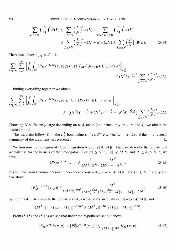
258 ROWAN KILLIP, MONICA VISAN AND XIAOYI ZHANG
XL��M
� L
M
�sM.L/�
XL��N
� L
N
�sM.L/C
X�N �L��M
� L
M
�sM.L/
.X
L��N
� L
N
�sM.L/C �sM.�N /.
XL��N
� L
N
�sM.L/: (5-14)
Therefore, choosing q D d C 1,
XM �N
1XkD0
ZR
ZRdŒPM e�it��.x;y/�k.t;y/Œ QPM F.u��M .t//�.y/ dy dt
L2
x
. .N 2ı/� d�2
dC1
XL��N
� L
N
�sM.L/:
Putting everything together we obtain
XM �N
1XkD0
ZR
ZRdŒPM e�it��.x;y/ �k.t;y/ Œ QPM F.u.t//�.y/ dy dt
L2
x
.u
�.N 2ı/�1C 2
d C .N 2ı/�1C 1d C .N 2ı/
� d�2dC1
� XL��N
� L
N
�sM.L/:
Choosing N sufficiently large depending on u, ı, and s (and hence only on u, �, and s), we obtain thedesired bound.
The last claim follows from the L2x-boundedness of �N P˙PM (see Lemma 4.2) and the time-reversal
symmetry of the argument just presented. �
We turn now to the region of .t;y/ integration where jyj � M jt j. First, we describe the bounds thatwe will use for the kernels of the propagators. For jxj � N �1, jyj � M jt j, and jt j � ı � N �2, wehave
jPM e�it�.x;y/j . 1
.M 2jt j/50d
M d
hM.x � y/i50dI (5-15)
this follows from Lemma 2.6 since under these constraints, jy � xj � M jt j. For jxj � N �1 and y andt as above,
jP˙M e�it�.x;y/j . 1
.M 2jt j/50d
M d
hM xid�1
2 hMyid�1
2 hM jxj � M jyji50d; (5-16)
by Lemma 4.1. To simplify the bound in (5-16) we used the inequalities jyj � jxj � M jt j and
hM 2jt j C M jxj � M jyji
�100d . .M 2jt j/�50d
hM jxj � M jyji�50d :
From (5-15) and (5-16) we see that under the hypotheses set out above,
jPM e�it�.x;y/j C jP˙M e�it�.x;y/j . 1
.M 2jt j/50dKM .x;y/; (5-17)

THE MASS-CRITICAL NONLINEAR SCHRÖDINGER EQUATION WITH RADIAL DATA 259
where
KM .x;y/ WDM d
hM.x � y/i50dC
M d
hM xid�1
2 hMyid�1
2 hM jxj � M jyji50d:
Note that by Schur’s test, this is the kernel of a bounded operator on L2x.R
d /.Let Q�k denote the characteristic function of the set˚
.t;y/ W 2kı � jt j � 2kC1ı; jyj � M jt j:
Lemma 5.5 (The tail). Let 0 < s < 1 C4d
, let � > 0 be a small number, and let ı be as in Lemma 5.3.Then X
M �N
1XkD0
ZR
ZRd
KM .x;y/
.M 2jt j/50dQ�k.t;y/ j QPM F.u.t//j.y/ dy dt
L2
x
�1
10
XL��N
� L
N
�sM.L/
for all N sufficiently large depending on u, s, and � (in particular, we require N � ı�1=2).
Proof. Using Holder’s inequality, the L2-boundedness of the operator with kernel KM , and Lemma 2.2, ZR
ZRd
KM .x;y/
.M 2jt j/50dQ�k.t;y/ j QPM F.u.t//j.y/ dy dt
L2
x
. .M 22kı/�50d .2kı/d�2
d M2.d�2/
d QPM F.u/
L
d2t L
2d2
d2C4d�8x .Œ2kı;2kC1ı��Rd /
. .M 22kı/�49d QPM F.u/
L
d2t L
2d2
d2C4d�8x .Œ2kı;2kC1ı��Rd /:
We decompose
F.u/D F.u��M /C O�ju��M j
4d ju>�M j
�C O
�ju>�M j
1C 4d
�: (5-18)
Discarding the projection QPM , we use Holder and (5-2) to estimate QPM O.ju��M j4d ju>�M j/
L
d2t L
2d2
d2C4d�8x .Œ2kı;2kC1ı��Rd /
. u��M
4d
L2t L
2dd�2x .Œ2kı;2kC1ı��Rd /
u>�M
L1
t L2x
.u h2kıi2d M.�N /; QPM O.ju>�M j
1C 4d /
L
d2t L
2d2
d2C4d�8x .Œ2kı;2kC1ı��Rd /
. u>�M
4d
L2t L
2dd�2x .Œ2kı;2kC1ı��Rd /
u>�M
L1
t L2x
.u h2kıi2d M.�N /:
To estimate the contribution coming from the first term on the right-hand side of (5-18), we use Lemma2.2, Corollary 2.5 (with r D d2=.d � 2/) combined with Holder’s inequality in the time variable, (5-2),

260 ROWAN KILLIP, MONICA VISAN AND XIAOYI ZHANG
and (5-14), to estimate QPM F.u��M /
L
d2t L
2d2
d2C4d�8x .Œ2kı;2kC1ı��Rd /
. M �s jrj
sF.u��M /
L
d2t L
2d2
d2C4d�8x .Œ2kı;2kC1ı��Rd /
. M �s jrj
su��M
L1
t L2x
u��M
4d
L2t L
2dd�2x .Œ2kı;2kC1ı��Rd /
.u h2kıi2d
XL��M
� L
M
�sM.L/.u h2kıi
2d
XL��N
� L
N
�sM.L/
for any M � N .Putting everything together, we deduce Z
R
ZRd
KM .x;y/
.M 2jt j/50dQ�k.t;y/ Œ QPMF.u.t//�.y/ dy dt
L2
x
. u .M22kı/�49d
h2kıi2d
XL��N
� L
N
�sM.L/:
Summing over k � 0 and M � N , we obtain
XM �N
1XkD0
ZR
ZRd
KM .x;y/
.M 2jt j/50dQ�k.t;y/Œ QPM F.u.t//�.y/ dy dt
L2
x
.u .N2ı/�49d
XL��N
� L
N
�sM.L/:
The claim follows by choosing N sufficiently large depending on ı, �, and s (and hence only on u, s,and �). �
Combining it all together:
Proof of Proposition 5.2. Naturally, we may bound ku�N kL2 by separately bounding the L2 norm onthe ball fjxj � N �1g and on its complement. On the ball, we use (5-7), while outside the ball we use(5-6). Invoking (5-8) and the triangle inequality, we reduce the proof to bounding certain integrals. Theintegrals over short times were estimated in Lemma 5.3. For jt j � ı, we further partition the region ofintegration into two pieces. The first piece, where jyj & M jt j, was dealt with in Lemma 5.4. To estimatethe remaining piece, jyj � M jt j, one combines (5-17) and Lemma 5.5. �
6. The double high-to-low frequency cascade
In this section, we use the additional regularity provided by Theorem 5.1 to preclude double high-to-lowfrequency cascade solutions. We argue as in [Killip et al. 2007].
Proposition 6.1 (Absence of double cascades). Let d � 3. There are no nonzero global sphericallysymmetric solutions to (1-1) that are double high-to-low frequency cascades in the sense of Theorem 1.10.
Proof. Suppose to the contrary that there is such a solution u. By Theorem 5.1, u lies in C 0t H 1
x .R�Rd /.Hence the energy
E.u/D E.u.t//D
ZRd
12jru.t;x/j2 C�
d
2.d C2/ju.t;x/j2.dC2/=d dx

THE MASS-CRITICAL NONLINEAR SCHRÖDINGER EQUATION WITH RADIAL DATA 261
is finite and conserved (see [Cazenave 2003], for example). Since M.u/ <M.Q/ in the focusing case,the sharp Gagliardo–Nirenberg inequality (Theorem 1.6) gives
kru.t/k2
L2x.Rd /
�u E.u/�u 1 (6-1)
for all t 2 R. We will now reach a contradiction by proving that kru.t/k2 ! 0 along any sequencewhere N.t/! 0. The existence of two such time sequences is guaranteed by the fact that u is a doublehigh-to-low frequency cascade.
Let � > 0 be arbitrary. By Definition 1.8, we can find C D C.�;u/ > 0 such thatZj�j�CN.t/
j Ou.t; �/j2 d� � �2
for all t . Meanwhile, by Theorem 5.1, u 2 C 0t H s
x.R � Rd / for some s > 1. Thus,Zj�j�CN.t/
j�j2sj Ou.t; �/j2 d� .u 1
for all t and some s > 1. Thus, by Holder’s inequality,Zj�j�CN.t/
j�j2j Ou.t; �/j2 d� .u �2.s�1/=s:
On the other hand, from mass conservation and Plancherel’s theorem we haveZj�j�CN.t/
j�j2j Ou.t; �/j2 d� .u C 2N.t/2:
Summing these last two bounds and using Plancherel’s theorem again, we obtain
kru.t/kL2
x.Rd /.u �
.s�1/=sC CN.t/
for all t . As � > 0 is arbitrary and there exists a sequence of times tn ! 1 such that N.tn/! 0 (u is adouble high-to-low frequency cascade), we conclude kru.tn/k2 ! 0. This contradicts (6-1). �
Remark. As mentioned in [Killip et al. 2007], the argument presented can be used to rule out nonradialsingle-sided cascade solutions that lie in C 0
t H sx for some s > 1. (By a single-sided cascade we mean
a solution with N.t/ bounded on a semiinfinite interval, say ŒT;1/, with lim inft!1 N.t/ D 0.) Forsuch regular solutions u, we may define the total momentum
RRd Im. Nuru/; which is conserved. By a
Galilean transformation, we can set this momentum equal to zero; thusZRd�j Ou.t; �/j2 d� D 0:
From this, mass conservation, and the uniform H sx bound for some s > 1, one can show that �.t/ ! 0
whenever N.t/! 0. On the other hand, a modification of the above argument gives
1 �u kru.t/k2 . �.s�1/=sC C
�N.t/C j�.t/j
�;
which is absurd.

262 ROWAN KILLIP, MONICA VISAN AND XIAOYI ZHANG
7. Death of a soliton
In this section, we use the additional regularity proved in Theorem 5.1 to rule out the third and finalenemy, the soliton-like solution. Once again, we follow [Killip et al. 2007]; the method is similar to thatin [Kenig and Merle 2006a]. Let
MR.t/ WD 2 ImZ
Rd
�jxj
R
�Nu.t;x/x � ru.t;x/ dx;
where is a smooth function obeying
.r/D
�1 if r � 1;
0 if r � 2;
and R denotes a radius to be chosen momentarily. For solutions u to (1-1) belonging to C 0t H 1
x , MR.t/
is a well-defined function. Indeed,
jMR.t/j . Rku.t/k2kru.t/k2 .u R:
An oft-repeated calculation (essentially that in the derivation of the Morawetz and virial identities) gives:
Lemma 7.1.
@tMR.t/D 8E.u.t//
�
ZRd
�d2�1
Rjxj 0
�jxj
R
�C
2d C1
R2 00
�jxj
R
�C
jxj
R3 000
�jxj
R
��ju.t;x/j2 dx (7-1)
C 4
ZRd
�
�jxj
R
�� 1 C
jxj
R 0
�jxj
R
��jru.t;x/j2 dx (7-2)
C4�
d C2
ZRd
�d
�
�jxj
R
�� 1
�C
jxj
R 0
�jxj
R
��ju.t;x/j
2.dC2/d dx; (7-3)
where E.u/ is the energy of u as defined in (1-3).
Proposition 7.2 (Absence of solitons). Let d � 3. There are no nonzero global spherically symmetricsolutions to (1-1) that are soliton-like in the sense of Theorem 1.10.
Proof. Assume to the contrary that there is such a solution u. Then, by Theorem 5.1, u 2 C 0t H s
x forsome s > 1. In particular,
jMR.t/j . u R: (7-4)
Recall that in the focusing case, M.u/ < M.Q/. As a consequence, the sharp Gagliardo–Nirenberginequality (Theorem 1.6) implies that the energy is a positive quantity in the focusing case as well as inthe defocusing case. Indeed,
E.u/&u
ZRd
jru.t;x/j2 dx > 0:
We will show that for R sufficiently large, (7-1) through (7-3) are small terms compared with E.u/.Combining this fact with Lemma 7.1, we conclude @tMR.t/& E.u/ > 0, which contradicts (7-4).
We first turn our attention to (7-1). This is trivially bounded as
j.7-1/j .u R�2: (7-5)

THE MASS-CRITICAL NONLINEAR SCHRÖDINGER EQUATION WITH RADIAL DATA 263
We now study (7-2) and (7-3). Let � > 0 be a small number to be chosen later. By Definition 1.8 andthe fact that N.t/D 1 for all t 2 R, if R is sufficiently large depending on u and �, thenZ
jxj� R4
ju.t;x/j2 dx � � (7-6)
for all t 2 R. Let � denote a smooth cutoff to the region jxj � R=2, chosen so that r� is bounded byR�1 and supported where jxj � R. As u 2 C 0
t H sx for some s > 1, using interpolation and (7-6), we
estimate
j.7-2/j . k�ru.t/k22 . kr.�u.t//k2
2 C ku.t/r�k22 . k�u.t/k
2.s�1/s
2ku.t/k
2s
H sx
C �.u �s�1
s C �: (7-7)
Finally, we are left to consider (7-3). Using the same � as above together with the Gagliardo–Nirenberginequality and (7-6),
j.7-3/j . k�u.t/k2.dC2/
d2.dC2/
d
. k�u.t/k4d2
kr.�u.t//k22 .u �
2d : (7-8)
Combining (7-5), (7-7), and (7-8) and choosing � sufficiently small depending on u and R sufficientlylarge depending on u and �, we obtain
j.7-1/j C j.7-2/j C j.7-3/j �1
100E.u/:
This completes the proof of the proposition for the reasons explained in the third paragraph. �
Acknowledgements
We are grateful to Shuanglin Shao for access to preliminary drafts of his work.
References
[Bégout and Vargas 2007] P. Bégout and A. Vargas, “Mass concentration phenomena for the L2-critical nonlinear Schrödingerequation”, Trans. Amer. Math. Soc. 359:11 (2007), 5257–5282. MR 2008g:35190 Zbl 05178492
[Berestycki and Lions 1979] H. Berestycki and P.-L. Lions, “Existence d’ondes solitaires dans des problèmes nonlinéaires dutype Klein–Gordon”, C. R. Acad. Sci. Paris Sér. A-B 288:7 (1979), A395–A398. MR 80i:35076 Zbl 0397.35024
[Blue and Colliander 2006] P. Blue and J. Colliander, “Global well-posedness in Sobolev space implies global existencefor weighted L2 initial data for L2-critical NLS”, Commun. Pure Appl. Anal. 5:4 (2006), 691–708. MR 2007f:35265Zbl 1137.35066
[Bourgain 1998] J. Bourgain, “Refinements of Strichartz’ inequality and applications to 2D-NLS with critical nonlinearity”,Internat. Math. Res. Not. 1998:5 (1998), 253–283. MR 99f:35184 Zbl 0917.35126
[Bourgain 1999a] J. Bourgain, Global solutions of nonlinear Schrödinger equations, American Mathematical Society Collo-quium Publications 46, American Mathematical Society, Providence, RI, 1999. MR 2000h:35147 Zbl 0933.35178
[Bourgain 1999b] J. Bourgain, “Global wellposedness of defocusing critical nonlinear Schrödinger equation in the radial case”,J. Amer. Math. Soc. 12:1 (1999), 145–171. MR 99e:35208 Zbl 0958.35126
[Carles 2002] R. Carles, “Critical nonlinear Schrödinger equations with and without harmonic potential”, Math. Models Meth-ods Appl. Sci. 12:10 (2002), 1513–1523. MR 2004b:35298 Zbl 1029.35208
[Carles and Keraani 2007] R. Carles and S. Keraani, “On the role of quadratic oscillations in nonlinear Schrödinger equations.II. The L2-critical case”, Trans. Amer. Math. Soc. 359:1 (2007), 33–62. MR 2008a:35260 Zbl 1115.35119

264 ROWAN KILLIP, MONICA VISAN AND XIAOYI ZHANG
[Cazenave 2003] T. Cazenave, Semilinear Schrödinger equations, Courant Lecture Notes in Mathematics 10, New York Uni-versity Courant Institute of Mathematical Sciences, New York, 2003. MR 2004j:35266 Zbl 1055.35003
[Cazenave and Weissler 1989] T. Cazenave and F. B. Weissler, “Some remarks on the nonlinear Schrödinger equation in thesubcritical case”, pp. 59–69 in New methods and results in nonlinear field equations (Bielefeld, 1987), edited by P. Blanchardet al., Lecture Notes in Phys. 347, Springer, Berlin, 1989. MR 91c:35136 Zbl 0699.35217
[Christ and Weinstein 1991] F. M. Christ and M. I. Weinstein, “Dispersion of small amplitude solutions of the generalizedKorteweg-de Vries equation”, J. Funct. Anal. 100:1 (1991), 87–109. MR 92h:35203 Zbl 0743.35067
[Colliander et al. 2002] J. Colliander, M. Keel, G. Staffilani, H. Takaoka, and T. Tao, “Almost conservation laws and globalrough solutions to a nonlinear Schrödinger equation”, Math. Res. Lett. 9:5-6 (2002), 659–682. MR 2003j:35294 Zbl 01930988
[Colliander et al. 2005] J. Colliander, S. Raynor, C. Sulem, and J. D. Wright, “Ground state mass concentration in the L2-critical nonlinear Schrödinger equation below H 1”, Math. Res. Lett. 12:2-3 (2005), 357–375. MR 2006e:35300 Zbl 1084.35088
[Colliander et al. 2007] J. Colliander, M. Grillakis, and N. Tzirakis, “Improved interaction Morawetz inequalities for thecubic nonlinear Schrödinger equation on R2”, Int. Math. Res. Not. 2007:23 (2007), Art. ID rnm090. Zbl 1142.35085arXiv math/0703606
[Colliander et al. 2008a] J. Colliander, M. Keel, G. Staffilani, H. Takaoka, and T. Tao, “Global well-posedness and scatteringfor the energy-critical nonlinear Schrödinger equation in R3”, Ann. of Math. .2/ 167:3 (2008), 767–865.
[Colliander et al. 2008b] J. Colliander, M. Keel, G. Staffilani, H. Takaoka, and T. Tao, “Resonant decompositions and the I -method for the cubic nonlinear Schrödinger equation on R2”, Discrete Contin. Dyn. Syst. 21:3 (2008), 665–686. MR 2399431Zbl 05304859
[De Silva et al. 2007a] D. De Silva, N. Pavlovic, G. Staffilani, and N. Tzirakis, “Global well-posedness and polynomial boundsfor the defocusing L2-critical nonlinear Schrödinger equation in R”, preprint, 2007. arXiv math/0702707
[De Silva et al. 2007b] D. De Silva, N. Pavlovic, G. Staffilani, and N. Tzirakis, “Global well-posedness for the L2 criticalnonlinear Schrödinger equation in higher dimensions”, Commun. Pure Appl. Anal. 6:4 (2007), 1023–1041. MR 2341818Zbl 05257774
[Fang and Grillakis 2007] Y. F. Fang and M. G. Grillakis, “On the global existence of rough solutions of the cubic defocusingSchrödinger equation in R2C1”, J. Hyperbolic Differ. Equ. 4:2 (2007), 233–257. MR 2008c:35303 Zbl 1122.35132
[Ginibre and Velo 1992] J. Ginibre and G. Velo, “Smoothing properties and retarded estimates for some dispersive evolutionequations”, Comm. Math. Phys. 144:1 (1992), 163–188. MR 93a:35065 Zbl 0762.35008
[Gradshteyn and Ryzhik 2000] I. S. Gradshteyn and I. M. Ryzhik, Table of integrals, series, and products, 6th ed., AcademicPress, San Diego, CA, 2000. Translated from the Russian. MR 2001c:00002 Zbl 0981.65001
[Kato 1995] T. Kato, “On nonlinear Schrödinger equations. II. H s-solutions and unconditional well-posedness”, J. Anal. Math.67 (1995), 281–306. MR 98a:35124a Zbl 0848.35124
[Keel and Tao 1998] M. Keel and T. Tao, “Endpoint Strichartz estimates”, Amer. J. Math. 120:5 (1998), 955–980. MR 2000d:35018 Zbl 0922.35028
[Kenig and Merle 2006a] C. E. Kenig and F. Merle, “Global well-posedness, scattering and blow-up for the energy-critical,focusing, non-linear Schrödinger equation in the radial case”, Invent. Math. 166:3 (2006), 645–675. MR 2007g:35232Zbl 1115.35125
[Kenig and Merle 2006b] C. E. Kenig and F. Merle, “Global well-posedness, scattering and blow-up for the energy criticalfocusing non-linear wave equation”, preprint, 2006. arXiv math/0610801
[Keraani 2001] S. Keraani, “On the defect of compactness for the Strichartz estimates of the Schrödinger equations”, J. Differ-ential Equations 175:2 (2001), 353–392. MR 2002j:35281 Zbl 1038.35119
[Keraani 2006] S. Keraani, “On the blow up phenomenon of the critical nonlinear Schrödinger equation”, J. Funct. Anal. 235:1(2006), 171–192. MR 2007e:35260 Zbl 1099.35132
[Killip and Visan 2008] R. Killip and M. Visan, “The focusing energy-critical nonlinear Schrödinger equation in dimensionsfive and higher”, preprint, 2008. arXiv 0804.1018

THE MASS-CRITICAL NONLINEAR SCHRÖDINGER EQUATION WITH RADIAL DATA 265
[Killip et al. 2007] R. Killip, T. Tao, and M. Visan, “The cubic nonlinear Schrödinger equation in two dimensions with radialdata”, preprint, 2007. arXiv 0707.3188
[Kwong 1989] M. K. Kwong, “Uniqueness of positive solutions of�u�uCup D 0 in Rn”, Arch. Rational Mech. Anal. 105:3(1989), 243–266. MR 90d:35015 Zbl 0676.35032
[Merle 1993] F. Merle, “Determination of blow-up solutions with minimal mass for nonlinear Schrödinger equations withcritical power”, Duke Math. J. 69:2 (1993), 427–454. MR 94b:35262 Zbl 0808.35141
[Merle and Tsutsumi 1990] F. Merle and Y. Tsutsumi, “L2 concentration of blow-up solutions for the nonlinear Schrödingerequation with critical power nonlinearity”, J. Differential Equations 84:2 (1990), 205–214. MR 91e:35194 Zbl 0722.35047
[Merle and Vega 1998] F. Merle and L. Vega, “Compactness at blow-up time for L2 solutions of the critical nonlinearSchrödinger equation in 2D”, Internat. Math. Res. Not. 1998:8 (1998), 399–425. MR 99d:35156 Zbl 0913.35126
[Nawa 1999] H. Nawa, “Asymptotic and limiting profiles of blowup solutions of the nonlinear Schrödinger equation withcritical power”, Comm. Pure Appl. Math. 52:2 (1999), 193–270. MR 99m:35235 Zbl 0964.37014
[Ryckman and Visan 2007] E. Ryckman and M. Visan, “Global well-posedness and scattering for the defocusing energy-criticalnonlinear Schrödinger equation in R1C4”, Amer. J. Math. 129:1 (2007), 1–60. MR 2007k:35474
[Shao 2007] S. Shao, “Sharp linear and bilinear restriction estimates for paraboloid in the cylindrically symmetric case”,preprint, 2007. arXiv 0706.3759
[Staffilani 1997] G. Staffilani, “On the generalized Korteweg-de Vries-type equations”, Differential Integral Equations 10:4(1997), 777–796. MR 2001a:35005 Zbl 0891.35135
[Stein 1993] E. M. Stein, Harmonic analysis: real-variable methods, orthogonality, and oscillatory integrals, Princeton Math-ematical Series 43, Princeton University Press, Princeton, NJ, 1993. MR 95c:42002 Zbl 0821.42001
[Stein and Weiss 1971] E. M. Stein and G. Weiss, Introduction to Fourier analysis on Euclidean spaces, Princeton Mathemat-ical Series 32, Princeton University Press, Princeton, N.J., 1971. MR 46 #4102 Zbl 0232.42007
[Strichartz 1977] R. S. Strichartz, “Restrictions of Fourier transforms to quadratic surfaces and decay of solutions of waveequations”, Duke Math. J. 44:3 (1977), 705–714. MR 58 #23577 Zbl 0372.35001
[Tao 2005] T. Tao, “Global well-posedness and scattering for the higher-dimensional energy-critical nonlinear Schrödingerequation for radial data”, New York J. Math. 11 (2005), 57–80. MR 2006e:35308 Zbl 1119.35092
[Tao 2006] T. Tao, “A pseudoconformal compactification of the nonlinear Schrödinger equation and applications”, preprint,2006. arXiv math/0606254
[Tao 2008a] T. Tao, “Global regularity of wave maps III”, preprint, 2008. arXiv 0805.4666
[Tao 2008b] T. Tao, “Global regularity of wave maps IV”, preprint, 2008. arXiv 0806.3592
[Tao 2008c] T. Tao, “Global regularity of wave maps V”, preprint, 2008. arXiv 0808.0368
[Tao et al. 2006] T. Tao, M. Visan, and X. Zhang, “Minimal-mass blowup solutions of the mass-critical NLS”, preprint, 2006.To appear in Forum Math. arXiv math/0609690
[Tao et al. 2007] T. Tao, M. Visan, and X. Zhang, “Global well-posedness and scattering for the defocusing mass-criticalnonlinear Schrödinger equation for radial data in high dimensions”, Duke Math. J. 140:1 (2007), 165–202. MR 2355070Zbl 05208403
[Taylor 2000] M. E. Taylor, Tools for PDE. Pseudodifferential operators, paradifferential operators, and layer potentials,Mathematical Surveys and Monographs 81, American Mathematical Society, Providence, RI, 2000. MR 2001g:35004 Zbl0963.35211
[Tsutsumi 1985] Y. Tsutsumi, “Scattering problem for nonlinear Schrödinger equations”, Ann. Inst. H. Poincaré Phys. Théor.43:3 (1985), 321–347. MR 87g:35221 Zbl 0612.35104
[Tzirakis 2005] N. Tzirakis, “The Cauchy problem for the semilinear quintic Schrödinger equation in one dimension”, Differ-ential Integral Equations 18:8 (2005), 947–960. MR 2006b:35306 Zbl 1075.35082
[Visan 2006] M. Visan, The defocusing energy-critical nonlinear Schrödinger equation in dimensions five and higher, PhDThesis, University of California, Los Angeles, 2006.
[Visan 2007] M. Visan, “The defocusing energy-critical nonlinear Schrödinger equation in higher dimensions”, Duke Math. J.138:2 (2007), 281–374. MR 2008f:35387 Zbl 1131.35081

266 ROWAN KILLIP, MONICA VISAN AND XIAOYI ZHANG
[Visan and Zhang 2007] M. Visan and X. Zhang, “On the blowup for the L2-critical focusing nonlinear Schrödinger equationin higher dimensions below the energy class”, SIAM J. Math. Anal. 39:1 (2007), 34–56. MR 2008b:35284 Zbl 1135.35079
[Weinstein 1983] M. I. Weinstein, “Nonlinear Schrödinger equations and sharp interpolation estimates”, Comm. Math. Phys.87:4 (1983), 567–576. MR 84d:35140 Zbl 0527.35023
[Weinstein 1989] M. I. Weinstein, “The nonlinear Schrödinger equation—singularity formation, stability and dispersion”, pp.213–232 in The connection between infinite-dimensional and finite-dimensional dynamical systems (Boulder, CO, 1987),edited by B. Nicolaenko et al., Contemp. Math. 99, Amer. Math. Soc., Providence, RI, 1989. MR 90m:35188 Zbl 0703.35159
Received 11 Aug 2008. Revised 20 Aug 2008. Accepted 23 Sep 2008.
ROWAN KILLIP: [email protected] Portola Plaza, Math Sciences Building 6363, Mailcode: 155505, Los Angeles, CA 90095, United Stateshttp://www.math.ucla.edu/~killip/
MONICA VISAN: [email protected] of Mathematics, University of Chicago, 5734 University Avenue, Chicago, IL 60637-1514, United Stateshttp://www.math.uchicago.edu/~mvisan/
XIAOYI ZHANG: [email protected] of Mathematics, Institute for Advanced Study, One Einstein Drive, Princeton, NJ 08540, United States

Guidelines for Authors
Authors may submit manuscripts in PDF format on-line at the Submission page at theAPDE website.
Originality. Submission of a manuscript acknowledges that the manuscript is original andand is not, in whole or in part, published or under consideration for publication elsewhere.It is understood also that the manuscript will not be submitted elsewhere while under con-sideration for publication in this journal.
Language. Articles in APDE are usually in English, but articles written in other languagesare welcome.
Required items. A brief abstract of about 150 words or less must be included. It shouldbe self-contained and not make any reference to the bibliography. If the article is not inEnglish, two versions of the abstract must be included, one in the language of the articleand one in English. Also required are keywords and subject classifications for the article,and, for each author, postal address, affiliation (if appropriate), and email address.
Format. Authors are encouraged to use LATEX but submissions in other varieties of TEX,and exceptionally in other formats, are acceptable. Initial uploads should be in PDF format;after the refereeing process we will ask you to submit all source material.
References. Bibliographical references should be complete, including article titles andpage ranges. All references in the bibliography should be cited in the text. The use ofBibTEX is preferred but not required. Tags will be converted to the house format, however,for submission you may use the format of your choice. Links will be provided to allliterature with known web locations and authors are encouraged to provide their own linksin addition to those supplied in the editorial process.
Figures. Figures must be of publication quality. After acceptance, you will need to submitthe original source files in vector graphics format for all diagrams in your manuscript:vector EPS or vector PDF files are the most useful.
Most drawing and graphing packages (Mathematica, Adobe Illustrator, Corel Draw, MAT-LAB, etc.) allow the user to save files in one of these formats. Make sure that whatyou are saving is vector graphics and not a bitmap. If you need help, please write [email protected] with details about how your graphics were generated.
White Space. Forced line breaks or page breaks should not be inserted in the document.There is no point in your trying to optimize line and page breaks in the original manuscript.The manuscript will be reformatted to use the journal’s preferred fonts and layout.
Proofs. Page proofs will be made available to authors (or to the designated correspondingauthor) at a Web site in PDF format. Failure to acknowledge the receipt of proofs or toreturn corrections within the requested deadline may cause publication to be postponed.