1 | P a g e

Analysing the efficiency of the Johannesburg

Stock Exchange using the Magic Formula

Christopher John Vincent

A thesis submitted to the Faculty of Commerce, Law and Management, Wits Business School

at the University of the Witwatersrand, Johannesburg, in partial fulfilment of the

requirements for the degree of Master of Management in the field of Finance & Investment.

Supervisor: Dr. Thanthi Mthanti

Signed on 27 February 2018 in Johannesburg

ii | P a g e

Abstract

This study examined the efficiency of South African markets, namely the Johannesburg Stock

Exchange (JSE) through the use of a value investing strategy called the “magic formula”, which

was created by Joel Greenblatt and published in his 2006 book “the little book that beats the

market”.

This study back tested the magic formula on the JSE from 2000 to 2016. It ranked stocks

according to the magic formula methodology, using earnings yield and return on capital to

derive portfolios.

The portfolios were then compared against the JSE All Share Index (the market). The magic

formula showed evidence of outperformance of the market over the period, even when

accounting for risk. The magic formula was compared against other portfolios derived from

value investing ratios, namely ROA, ROE and EY. The ROA portfolio produced the best risk-

adjusted results, but all value investing portfolios outperformed the market providing

evidence against efficient markets.

iii | P a g e

List of Tables

Table 3.1: Magic Formula Results 26

Table 4.1: Portfolio Construction 37

Table 5.1: Key statistics of Portfolio A versus the Market 44

Table 5.2: Key statistics of Portfolio B versus the Market 46

Table 5.3: Key statistics of Portfolio A versus Portfolio B 48

Table: 5.4 Key Statistics for the Magic Formula and Various Market Indexes 65

Table 5.5: Key statistics for the alternative portfolios, Portfolio B and the market 53

Table A: Portfolio A Results versus the Market 63

Table B: Portfolio B Results versus the Market 64

Table C: Alternative investment strategies 66

List of Figures

Figure 4.1: Market capitalization percentage of JSE listed shares 32

Figure 4.2: Purchase and sale representation 38

Figure 5.1: Graphical representation of Portfolio A versus the Market 42

Figure 5.2: Cumulative returns Portfolio A versus the Market 44

Figure 5.3: Graphical representation of Portfolio B versus the Market 45

Figure 5.4: Cumulative returns Portfolio A versus the Market 47

Figure 5.5: Graphical representation of all annualized returns 49

Figure 5.6: Cumulative returns for Portfolio A, B, and the various indexes 51

Figure 5.7: Graphical representation of all annualized returns 52

Figure 5.8: Cumulative returns for alternative portfolios, Portfolio B and the market 54

iv | P a g e

List of Acronyms and Abbreviations

B/M Book-to-Market

C/P Cash Flow-to-Price

D/P Dividend-to-Price

Dt Dividend at time t

EBIT Earnings Before Interest and Tax

EMH Efficient Market Hypothesis

EY Earnings Yield

JSE Johannesburg Stock Exchange

N Number of periods

NCAV Net Current Asset Value

NYSE New York Stock Exchange

P/E Price/Earnings

Pt Stock Price at time t

Pt-1 Stock price at time t-1

R Annual Return

ROA Return on Assets

ROC Return on Capital

ROE Return on Equity

𝑅market Annualized Return of the market

𝑅portfolio Annualized Return of the portfolio

Rrisk-free Risk-free rate

S&P 500 Standard and Poor’s 500 index

SG Share Group

UK United Kingdom

US United States

VAR market Variance of the market

VAR portfolio Variance of the portfolio

v | P a g e

Table of Contents Abstract…………………………………………………………………………………………………………………………………………….ii

List of Tables…………………………………………………………………………………………………………………………………….iii

List of Figures……………………………………………………………………………………………………………………………………iii

List of Acronyms and Abbreviations…………………………………………………………………………………………………iv

Table of Contents………………………………………………………………………………………………………………………………v

CHAPTER 1 INTRODUCTION .................................................................................................................... 1

CHAPTER 2 LITERATURE REVIEW ............................................................................................................ 5

2.1 Efficient Market Hypothesis .................................................................................................... 5

2.2 Misconceptions surrounding the EMH ................................................................................... 7

2.3 Behavioural Finance and Contradictions of the EMH. ............................................................ 9

2.3.1 Low Price to Earnings (P/E) Ratio .................................................................................. 10

2.3.2 Book-to-Market (B/M) ratio .......................................................................................... 12

2.3.3 Dividend-to-price (D/P) ratio ........................................................................................ 12

2.3.4 Turn-of-the-Year Effect/January Effect: ........................................................................ 13

2.3.5 Size effect ...................................................................................................................... 15

2.3.6 Weekend Effect: ............................................................................................................ 15

2.3.7 Momentum and Contrarian Strategies/Effects ............................................................ 17

2.4 Value investing as investment strategy ................................................................................ 19

2.5 Conclusion ............................................................................................................................. 22

CHAPTER 3 GREENBLATT’S MAGIC FORMULA ...................................................................................... 23

3.1 Introduction .......................................................................................................................... 23

3.2 The Magic Formula ............................................................................................................... 23

3.3 Greenblatt’s ranking system ................................................................................................. 25

3.4 Results ................................................................................................................................... 26

3.5 Greenblatt versus the EMH ................................................................................................... 28

3.5.1 Mispricing of risk ........................................................................................................... 28

3.5.2 The size effect ............................................................................................................... 28

3.5.3 Looking ahead bias ........................................................................................................ 29

3.5.4 Survivorship bias ........................................................................................................... 29

3.5.5 Data mining ................................................................................................................... 29

CHAPTER 4 RESEARCH METHODOLOGY ............................................................................................... 31

4.1 Introduction .......................................................................................................................... 31

4.2 Data Collection and Processing ............................................................................................. 31

vi | P a g e

4.3 Avoiding Statistical Bias ........................................................................................................ 34

4.4 Methods: ............................................................................................................................... 35

4.5 Calculating Returns ............................................................................................................... 39

4.6 Accounting for Risk ............................................................................................................... 40

CHAPTER 5 FINDINGS ............................................................................................................................ 42

5.1 Introduction: ......................................................................................................................... 42

5.2 Portfolio A and Portfolio B performance versus the Market ................................................ 42

5.3 Portfolio A versus Portfolio B ................................................................................................ 47

5.4 The Magic Formula (Portfolio A and B) versus various other Market Indexes ..................... 49

5.5 The Magic Formula versus alternative value investing portfolios ........................................ 52

CHAPTER 6 CONCLUSION ...................................................................................................................... 55

6.1 Conclusion ............................................................................................................................. 55

6.2 Further Research ................................................................................................................... 56

References ............................................................................................................................................ 57

Appendix 1: ....................................................................................................................................... 63

Appendix 2: ....................................................................................................................................... 64

Appendix 3: ....................................................................................................................................... 65

Appendix 4: ....................................................................................................................................... 66

1 | P a g e

CHAPTER 1

INTRODUCTION

1. Introduction

The goal of any investment is to earn a return and save for future spending; in other words,

forgo current consumption in the hopes of greater future consumption. Many investors

strongly believe they can systematically beat the market and earn superior returns through

exploiting market inefficiencies and optimal stock selection strategies (Coval, Hirshleifer &

Shumway, 2005). But can you systematically beat the market? This has been a long and

frequently debated question amongst practitioners and academics alike (Persson & Selander,

2009).

The Efficient Market Hypothesis (EMH) which sprang to popularity in the 1970s suggests and

provides evidence that you cannot beat the market for a prolonged period (Degutis &

Novickyte, 2014). A simple summation for this is that, all information is already fully reflected

in stock prices and thus unless you had insider information or take greater risks you would

not be able to beat the market. While the EMH is widely accepted investors such as, Warren

Buffet and Peter Lynch have outperformed the market for decades now. Warren Buffet has

delivered returns of 155 times that of the S&P 500 over a period of 52 years (Frankel, 2017).

Peter Lynch, also outperformed the S&P500 in all but two years from 1977 to 1990, averaging

annual returns of 29% versus the S&P500 return of 8.35% (Frankel, 2010). The fact that so

many investment houses and stock brokers exist, that individuals and institutions a like

continue to try earn superior returns suggest that the EMH does not satisfy all.

Many different investment strategies have been developed over the years such as, value

investing, growth investing, contrarian investing and momentum investing to mention a few.

2 | P a g e

These strategies all believe that they can identify anomalies of the EMH and take advantage

of the inefficiencies they create in markets. This thesis has a strong focus on investing

strategies and specifically Joel Greenblatt’s Magic Formula, outlined in his book called: The

little book that beat the market.

Studies by Njanike (2010) and Mabhunu (2004) state that the JSE is an efficient market and

abides by the notions of the EMH. If this is the case, then alternative investing strategies will

not yield returns greater than that of the market. Similarly, the concept should hold for the

United States (US) market which is believed to be efficient, yet Greenblatt (2006) claims to

have systematically beaten market returns from 1988 to 2004. Hoffman (2012), studied stock

market anomalies on the JSE between 1985 and 2010 and found strong evidence of said

anomalies and concluded that the JSE was not efficient, at least not strong or semi-strong

form.

The magic formula is based on simple principles and identifies value through information

available to all participants in the market. If market outperformance occurs it will provide

strong evidence of inefficient markets, or at least support the Hoffman’ (2012) notion that

strong and semi-strong form efficiency doesn’t exist. It will also provide evidence that the

formula works in developing economies and not just the US.

Joel Greenblatt created a formula for stock selection whereby he identified stocks that he

believed were undervalued in the market and would grow as investors realized the same.

From this he built portfolios of 30 stocks, where he would buy stocks on a rolling basis and

sell them exactly one year from their purchase date. Following the method outlined by him

in the little book that beat the market he claims to have earned far superior returns to the

3 | P a g e

market over the course of 17 years. Not only did he earn superior returns he also claimed to

have had lower risk. Greenblatt identifies risk different to most, he claims it is the number of

negative returns and not necessarily the variance of returns.

The purpose of this report is to investigate the EMH, value investing, and specifically back test

Joel Greenblatt’s Magic Formula in South Africa, using the companies listed on the

Johannesburg Stock Exchange (JSE) from 1 January 2000 to 31 March 2016. The annualized

return generated from these portfolios will then be benchmarked against the JSE All Share

Index, the JSE Value Index, the JSE Basic Materials Index, the JSE Growth Index, the JSE Small

Cap Index and the JSE Equally Weighted Top 40 Index. This determined if the portfolios would

beat the market.

To determine if markets were efficient in South Africa, three ratios often used to identify value

in stocks were selected to create new portfolios, these were Return on Assets (ROA), Return

on Equity (ROE) and Earnings Yield (EY). ROA is a profitability ratio that provides investors

with an indication of how efficiently a business is using its assets to generate profit (Dao,

2016). ROE is another profitability ratio that lets investors know how well a company is

generating revenue with shareholder’s investments (Dao, 2016). EY provides investors with a

means to measure returns and allows investors to evaluate if the returns commensurate for

risk (Dao, 2016). The returns from these portfolios were then compared to the returns

generated by the market and the magic formula to determine market efficiencies and the

optimal value investing strategy.

The rest of this study is divided into five more chapters and is constructed as listed: Chapter

two is a comprehensive literature review of previous research done on the topics. Chapter

three defines the Magic Formula, how it is constructed and how it performed as stated by

4 | P a g e

Greenblatt. Chapter four outlines the research methodology and data collection process.

Chapter five presents the findings of the report. Chapter six concludes the report and

proposes potential areas for future research.

5 | P a g e

CHAPTER 2

LITERATURE REVIEW

2.1 Efficient Market Hypothesis

The Efficient Market Hypothesis (EMH) is a largely debated investment theory that states it is

impossible for an investor to continuously deliver a return above that of the market as a result

of market efficiency (Olin, 2011).

An efficient market exists when all available information, as well as, the cumulative

knowledge of investors is reflected in stock market prices (Perrson and Selander, 2009). The

result of which would be shares always trading at their fair value, making the purchase of

undervalued shares and selling of overvalued shares an impossibility. As such, expected

returns on equity are merely a function of risk, rendering expert stock selection and market

timing ineffective (Olin, 2011). Because all investors have the same information and stocks

trade at their fair values, investors would not be able to earn a premium on market returns

without taking on additional risk (Howard, 2015).

The concept of market efficiency, which originated in the 19th century, reached the height of

its academic popularity in the nineteen eighties but its popularity and validity has been

declining since (Degutis & Novickytė, 2014). The roots of efficient market theory trace back

as far as 1889, to a man by the name of George Gibson. He wrote that when “shares become

publicly known in an open market, the value which they acquire may be regarded as the

judgment of the best intelligence concerning them” (Gibson, 1889). Thus, markets price

stocks relative to the opinions of the smartest market participants. Gibson (1889) was of the

belief that valuation of stocks is a voting game, where all market participants would vote on

whether stock prices should rise or fall (De Moor, Van den Bossche, & Verheyden, 2013). The

6 | P a g e

“Smartest participants would eventually gain more votes for their correct guesses which

would allow them to accumulate more funds” (Degutis & Novickytė, 2014).

In 1933 and 1944 US economist A. Cowles analyzed trade statistics of professional investors

and was able to conclude that investors were in fact unable to predict future stock prices in

order to earn excess profits (Degutis & Novickytė, 2014). The year 1953 saw Maurice Kendall

publish his work on stock and commodity prices, which found that prices did not move in

regular cycles but rather followed a random walk (Persson & Stahlberg, 2006). 12 years later

Professor Eugene Fama of the University of Chicago was able to confirm that stock prices were

in fact random and defined the “efficient market” concept for the first time (Fama, 1965). It

was H. Roberts who coined the term “Efficient Market Hypothesis” and separated markets

into strong and weak form (Sewell, 2011). The EMH as we know it today was formulated and

published by Fama in 1970 and included three forms of EMH: strong form, semi-strong form

and weak form (Fama, 1970).

The strong form of the EMH states that prices reflect all private and public information, even

information that is only accessible to company insiders (Persson & Stahlberg, 2006). Under

strong form efficiency not even company insiders would be able to make abnormal profits

and insider trading would essentially not exist. This level of efficiency is not meant to

represent reality but is rather a benchmark created to measure the importance of deviation

from an efficient market (Olin, 2011).

The semi-strong form of the EMH states that prices adjust rapidly to new information entering

the market and all information available publically is reflected in share prices. This form of the

EMH states one cannot continuously outperform the market using either technical or

fundamental analysis (Howard, 2015).

7 | P a g e

The weak form of the EMH infers that all historical information and stock prices are reflected

in current stock prices. In other words, stock prices reflect all information that can be derived

by examining the markets trading data (Guo & Wang, 2007). This in turn renders technical

analysis (trend analysis) ineffective and unlikely to produce abnormal returns, as historical

stock price data would be readily available to the market and would essentially be costless. If

the data did present reliable signals about the potential future profits, investors would have

learned to exploit these signals, which would result in these signals losing their value as they

become universally known by investors (Guo & Wang, 2007). Fundamental analysis on the

other hand has the potential to contribute to excess returns.

2.2 Misconceptions surrounding the EMH

(i) The first misconception is that investors are unable to beat the market.

The EMH does not state that investors cannot beat the market but rather that they should

not expect to consistently deliver or earn returns abnormal to that of the market. Clark, Jandik

& Mandelker (2001) state that in fact investors could make abnormal returns for a prolonged

period just by chance.

(ii) The second misconception claims attempts to perform financial analysis will not

result in superior returns because all investors are exposed to the same information

and attempting security selection is frivolous (Persson & Stahlberg, 2006). Malkiel

(1973) states “a blindfolded chimpanzee throwing darts at the Wall Street Journal

could select a portfolio that would do as well as the experts”. Financial

professionals have not lost their places in financial markets, which imply their

8 | P a g e

services are valuable or at least perceived as valuable. Critics thus argue that the

EMH must be invalid (Clark, Jandik & Mandelker, 2001).

The EMH does not dispute that different individual investors will have different investing

preferences (Howden, 2009). Some investors will be willing to invest in high-risk strategies,

while others will only be willing to invest in low-risk strategies. Finance professionals should

provide investors with portfolios that match the risk and return requirement of each

individual investor (Clark, Jandik & Mandelker, 2001). Another important point to note here

is that financial analysis itself is far from pointless in efficient markets. Efficient markets are

in hindsight created by the competition amongst investors who are analyzing information to

take advantage of mispriced securities. Clark, Jandik & Mandelker, (2001) describe financial

analysis as the engine that allows new information to rapidly filter into stock prices. Howden

(2009) goes further in stating that professionals can gain from their analysis, but there is a

cost incurred with analysis and these gains will not be sufficient to compensate for the added

costs.

(iii) The third misconception pertaining to the EMH is that new information cannot be

fully reflected in the market prices because prices fluctuate constantly.

Many observers view the fluctuations as the absence of new information, when in reality new

information pertaining to securities enters the markets constantly causing these fluctuations

in price (Howden, 2009). Instead of viewing price adjustments as market inefficiency, it should

rather be viewed as a market operating in an efficient manner. (Clark, Jandik & Mandelker,

2001).

9 | P a g e

(iv) The fourth misconception of the EMH is that it is incorrect; it assumes that all

investors have similar skills and ability to analyze information. This is not true and

in fact many investors are essentially layman and not financial experts (Clark,

Jandik & Mandelker, 2001).

While not all investors are skilled professionals, market efficiency can be achieved if only a

fraction of core skilled investors are well informed (Howden, 2009).

2.3 Behavioural Finance and Contradictions of the EMH.

The EMH is widely accepted as valid and was once touted as the most empirically supported

proposition in economics, but more recent research has questioned its robustness (Sewell,

2011). This is not surprising given the EMH questions professional investors’ ability to detect

mispriced securities.

The EMH is built on three preconditions: (i) there are no transaction costs incurred when

trading (ii) information is publicly available and costless and (iii) the pricing implications from

current information entering the market is agreed upon by those participating in the market

(Guo & Wang, 2007). The EMH states that because these three conditions are present all

investors will act in a rational manner (Fama, 1970).

By the beginning of the twenty first century the EMH was losing favour, with many finance

professionals believing that stock prices were to some degree predictable (Malkiel, 2003).

Malkiel (2003) argues that there are numerous cases in market history which support the

notion that market prices were not set by rational investors. One such case can be seen by

the pricing of stocks during the internet stock boom of the early 2000’s. Another would be

10 | P a g e

the stock crash of October 1987, whereby stock markets lost one third of their value overnight

(Malkiel, 2003).

The EMH has been described by some as the most significant error in the history of economics

(Malkiel, 2011). Several patterns contradicting the EMH, known as anomalies, have been

identified. These anomalies have given rise to what is known as Behavioural Finance,

behavioural theorists believe that investors do not behave rationally but are rather irrational

when making investing decisions. They believe this irrational behavior is generating the

opportunity for stock market anomalies to occur and results in abnormal returns (Howard,

2015). Shiller (2003) describes behavioural finance as looking at finance from a psychological

and social perspective in an attempt to understand why investors do not act rationally.

As the world moves to increased knowledge sharing, improved legislation surrounding

financial reporting and easier access to such information via improved technological

infrastructure these anomalies seem to be fading out. The section below will interrogate

some of the more researched and reported anomalies that have emerged because of

behavioural finance.

2.3.1 Low Price to Earnings (P/E) Ratio

The Price-earnings ratio (P/E) is the most widely used earnings multiple and articulates what

an investor will pay for one dollar of a company’s earnings (Persson and Stahlberg, 2006). This

is calculated by dividing the current market price of a share by the earnings generated per

share (Persson and Stahlberg, 2006). Basu (1977) set out to test whether earnings ratios

provide indications of future performance.

11 | P a g e

Basu’s (1977) set out to determine if stocks performance is linked to their P/E ratio. His

research compiled data from more than 1400 listed or delisted industrial firms on the New

York Stock Exchange (NYSE) from September 1956 to August 1971. Basu (1977) found that on

average low P/E portfolios outperformed high P/E portfolios and the market, even when

adjusting for risk. Rather than interpreting his results as a failure of the EMH he theorises that

information does not reflect quickly enough to satisfy semi-strong form or strong form

efficiency. He states it was because of this that markets remained in disequilibrium for the

period under study (Basu, 1977). Basu (1977) interpreted high P/E ratios as indicating

investors having confidence in future earnings and that these expectations are exaggerated

and slow to react. He goes further to explain that these lags are part of the general market

mechanism and that the anomaly did exist during the period under study, however,

transaction costs and taxes significantly impeded investors from yielding excess returns (Basu,

1977).

Reinganum (1981) proved that the P/E effect disappears when it is considered in conjunction

with the size effect, whereas Jaffe, Keim and Westerfield (1989) found that both the P/E ratio

and the size effect are significant.

Fama and French (1992) argue that low P/E ratio stocks carry more risk. Whereas, Lakonishok,

Shleifer and Vishny (1994), prove that low P/E portfolios like other value investing portfolios

produce abnormal returns through exploiting suboptimal investor behaviour and not due to

additional risk.

12 | P a g e

2.3.2 Book-to-Market (B/M) ratio

This is an anomaly whereby firms with high book value of firm equity (B) to market value of

firm equity (M) provide abnormal returns to investors. The anomaly was first discovered by

Stattman (1980) who found a return premium for US stocks with a high B/M value.

Fama and French (1992) determined that both B/M and size anomalies explained most

variation in US stock returns. Fama and French (1993) hold the stance that B/M and size

effects are purely compensating investors for holding riskier assets. Haugen (1995) finds

differently, he argues that it is not risk compensation but rather investors using past

performance to infer too far into the future regarding stock performance. It is this inference

that results in markets under-pricing high B/M firms (value shares) and overpricing low B/M

firms (growth shares). Daniel and Titman (1997) believe the B/M effect to be a result of

investor preference for growth stocks over those of value stocks.

2.3.3 Dividend-to-price (D/P) ratio

As is the case with P/E, D/P is a measure of value which is frequently used in practice and in

academia to try predict future stock prices. The D/P ratio is derived by dividing the dividend

by the current stock price. Campbell and Shiller (1988) found evidence to suggest that the

initial dividend outlay made by a company is a good predictor of the variance in future stock

prices or rather returns of said stock. Campbell and Shiller (1988) have shown that investors

who buy a basket of equities with high initial dividends have earned abnormal returns to that

of the market.

Stocks that pay high dividends yields outperform stocks that provide investors with lower

yields. This makes sense as investors are looking for returns and capital gains are not certain

13 | P a g e

or tangible until the stocks are sold. Companies that provide higher dividends yields are likely

to continue doing so in the near future, as changing their dividend policy could send signals

to the market which could negatively affect stock prices.

Fluck, Malkiel and Quandt (1997) argue that this may not be the case when picking individuals

stocks. Malkiel (2003) proved that dividend yields have not being able to predict future

earnings since the eighties. It has been argued that this may have been caused as a result of

changing dividend policies of companies, which now make extensive use of share buy backs

as a means to pay shareholders (Fama & French , 2001). This train of thought suggests that

the D/P ratio may no longer be a useful predictor of future earnings.

2.3.4 Turn-of-the-Year Effect/January Effect:

This is the phenomenon whereby share prices tend to appreciate and the volumes of shares

traded increase during the turn-of-the-year, resulting in January having greater returns than

in other months (Yavrumyan, 2015). The turn-of-the-year refers to the very last week of the

year and the first two weeks of a New Year.

Guo and Wang (2007) showed that returns for the rest of the year averaged 0.42% while

January produced returns of 3.48%, this showing the turn-of-the-year effect is in fact a

January effect. Rozeff and Kinney (1976) conducted empirical studies based on the NYSE

which confirmed the January effect between 1904 and 1974. They found that on average

returns were seven times higher in comparison to other months.

Keim (1983) while conducting a study on the size effect found that small-size firms excess

stock returns were not obtained evenly throughout time. Research by Jordan, Miller & Dolvin

14 | P a g e

(2015) showed that most of the abnormal returns for small-sized firms over that of large-sized

firms occurred in January, especially near the turn-of-the-year.

Numerous researchers have hypothesised why the January effect exist, two of the main

theories are: the information hypothesis and the tax-loss selling hypothesis (Guo and Wang,

2007).

The tax-selling hypothesis states investors tend to offload underperforming stocks late in the

year to drive up capital losses and lower the tax liability they incur. The consequence of such

action is that the poorly performing stocks face downward pressure on prices. This downward

pressure however disappears at the beginning of the next year in the absence of selling

pressure allowing stock prices to normalize (Guo and Wang, 2007). Roll (1983) found that

small-sized firms will be more affected by the tax-loss selling than big-sized firms.

Evidence has suggested that tax while a strong explanatory variable may not be alone in

explaining the January effect. Thaler (1987) identified the January effect in both Great Britain

and Australia even though their tax years do not occur in January. Ho (1990) provided

evidence that most Asian countries do not experience the January effect. Only 3 of 9 countries

under investigation experienced a tax effect. Thaler (1987) and Brown, Kleidon, & Marsh

(1983) were able to show that returns were abnormally high for the countries under study

during the start of a new tax year, proving tax can help explain the excess returns experienced

but it is not the only explanatory variable.

One such explanatory variable could be the release of new information and the uncertainty

that it creates, more commonly known as the information hypothesis (Persson and Selander,

2009). Keim (1983) states the information hypothesis would have a greater effect on small-

15 | P a g e

sized firms. This is because publishing of such information is easier, more cost effective and

less onerous than for that of large-sized firms.

2.3.5 Size effect

Banz (1981) studied the relationship between the market value of shares on the NYSE and

returns they generated. He found that the stocks of small firms earned higher returns than

stocks of large firms after accounting for risk between the years 1936 to 1975. This finding

became known as the size effect.

Herrera and Lockwood (1994) found a monthly premium of 4.16% for small stocks on the

Mexican stock exchange. A similar premium has been found in Japan, which showed a size

premium of 1.2% (Ziemba, 1991).

It was Klein and Bawa (1977) that determined small firms often have a scarcity of information

available and this led to investors having less desire to hold these stocks because of estimation

risk. Recent studies such as the one done by Horowitz, Loughran, and Savin (2000) have

suggested that this effect has all but vanished since the eighties. They examined average stock

return data between 1982 and 1997 and found no signs of it.

2.3.6 Weekend Effect:

This is the phenomenon within financial markets whereby stocks have significantly lower

prices on Monday’s than they did at the close of the preceding Friday (Yavrumyan, 2015).

Calculating a daily return on the stock market is accomplished by taking the change in closing

price from one trading day to the next as a percentage. This would entail a 24-hour period for

each day in the week except Monday which would include the weekend and result in a 72-

16 | P a g e

hour period. This longer period would lead one to believe that Monday’s should have the

highest returns but it in fact has the lowest average return (Jordan, Miller & Dolvin, 2015).

Various authors believe Monday’s tend to produce relatively large negative returns for

financial assets. Howard (2015) states that this is due negative news/information about

companies being released on weekends. It was French (1980) who theorised companies

release negative information on weekends in order to avoid panicked sales of their shares.

Miller (1988) was of the belief that trading patterns of individual investors resulted in what is

now known as the weekend effect. He believed individuals followed brokerage communities

to make buy decisions on working/weekdays, then on weekends when time allowed they

would review their positions and make sell decisions to adjust portfolios on the Monday.

This anomaly was originally referred to as the Monday effect (Cross, 1973). French (1980)

showed that between 1953 and 1977 many of the negative returns where a result of non-

trading periods from Friday-close to Monday-open. Similar results were found by Keim and

Stambaugh (1984) for the period 1928 to 1952. It was these arguments that confirmed the

Monday effect was in fact the weekend effect (Howard, 2015). The weekend effect is quite

possibly the strongest calendar anomaly, but it is not sufficient enough to support an entire

trading strategy alone (Persson and Selander, 2009).

The weekend effect appears to have disappeared after 1987. In fact, Rubenstein (2001)

highlights that between the years 1989 to 1998 Monday produced the highest returns of any

trading day. This would indicate that the weekend effect no longer exist (Rubenstein, 2001).

17 | P a g e

2.3.7 Momentum and Contrarian Strategies/Effects

These are strategies where success is derived from a shares past performance in comparison

to a given benchmark, this is in contradiction to the random walk hypothesis and market

efficiencies.

2.3.7.1 Contrarian Strategy

This strategy is derived off the back of behavioural psychology, which tells us that when

making investment decisions people do not behave in a rational manner because they

overreact to unexpected/recent information, good or bad. This in turn will lead to a stock

market overreaction to said news, with stock prices rising (falling) too far but eventually

returning to their intrinsic value upon investors realising they overreacted (Hamalainen,

2007). De Bondt and Thaler (1985) referred to this as the contrarian effect whereby, investors

overreact to recent news and respond by selling loser shares below their intrinsic value and

buying winner shares at a premium. Contrarian investors take advantage of this situation by

investing in the undervalued shares and selling of overpriced shares, thus allowing them to

earn returns above that of the market (Lakonishok, Shleifer, & Vishny, 1994).

It was De Bondt and Thaler (1985) who first investigated this return reversal phenomenon in

stock markets. They constructed winner and loser portfolios using monthly data consisting of

all stocks on the NYSE for the period between 1926 and 1982. A stock was labelled a winner

or loser based on its past performance, ranging from one to five years (Howard, 2015). They

ranked stocks according to their cumulative returns in descending order to create what would

be winner and loser portfolios. The winner portfolios consisted of the top 35 shares and the

loser portfolio of the bottom 35 shares. (Hamalainen, 2007). A three to five-year period was

then used to measure the performance of these portfolios (Persson and Selander, 2009). The

18 | P a g e

result was that losers out performed winners by roughly 24% over the next three-year period

and roughly 32% over the next five-year period (De Bondt and Thaler, 1985). The most

peculiar result was that winners were significantly riskier than losers.

While many accept the findings De Bondt and Thaler (1985), Conrad and Kaul (1993) dispute

these findings stating they are not valid. Conrad and Kaul (1993) studied a sample of stocks

listed on the NYSE between 1926 and 1988 and found that winner portfolios outperformed

losers’ portfolios by 1.7%. Kryzanowski and Zhang (1992) suggest that the contrarian effect is

only applicable when applied to U.S. markets. They applied the framework defined by De

Bondt and Thaler (1985) to the markets in Canada and were not able to produce results that

proved the hypothesis. Baytas and Cakici (1999) found similar results to Kryzanowski and

Zhang (1992) when applying a similar framework to various industrialised countries such as,

Canada, UK, Japan, Germany, France and Italy.

2.3.7.2 Momentum Strategy

A momentum strategy unlike the contrarian sells past losers and buys past winners.

Momentum investing is a strategy whereby the investors are not concerned with meticulous

analysis of a company’s performances or share price but rather with monitoring what other

parties in the market are doing (Beunza & Stark, 2004). It strays away from attempts to

understand the stock’s value instead they focus on if stocks are going up or down in the

market – the identifications of trends (Hamalainen, 2007). They believe that momentum is a

self-fuelling social process that can be understood through study and profited from.

Despite the contrarian effect and evidence found regarding the topic, many mutual funds to

this day buy shares on an upward trend from the previous quarter (Hamalainen, 2007). Levy

19 | P a g e

(1967) was the first to study the momentum effect, but his results were found to be

controversial.

Jegadeesh and Titman (1993) were the first study to provide evidence of momentum

strategies providing excess returns. Their study used data from 1965 to 1989 and the strategy

that they implemented was to buy shares performing well in the last 12 months and sells

those that had performed poorly. What they proved was that a momentum strategy will

produce abnormal returns in the first 12 month holding period, but they found that these

returns tend to dissipate over a 24-month holding period (Jegadeesh and Titman, 1993).

Moskowwitz and Grinblatt (1999) not only confirmed the existence of the momentum effect

but went one step further in determining that the effect is stronger when viewed per industry,

rather than by individual stock.

Unlike the contrarian effect the momentum effect seems to be consistent across countries

and not just in the U.S. Rouwenhorst (1998) studied the momentum effect between 1978 and

1995 within 12 countries in Europe using a data set of just below 2200 companies. He showed

that the excess return of winner over loser portfolios was 1.16% per month. When

Rouwenhorst (1998) tested the 12 European countries separately, he found that 11 of the 12

countries showed evidence of the momentum effect.

2.4 Value investing as investment strategy

Value investing is the school of thought by which investors buy a share at a low price and sell

it at a higher price (Beunza & Stark, 2004). An investor believes that through fundamentals

analysis, such as a reviewing a company’s annual financial statements, they can identify and

purchase stocks that are on the market at a price below that of their intrinsic value (Howard,

20 | P a g e

2015). This is the opposite of Growth investing, whereby investors believe in the principles of

the EMH and purchase stocks that have shown fast or consistent growth (Howard, 2015).

Importantly, value investors believe that “property” has intrinsic value that is entirely

independent of other investor’s views or perspectives. It is their belief that markets are

inefficient but that this mispricing or inefficiency will eventually be corrected (Basu, 1977). In

other words, markets will slowly realize a security is mispriced increasing demand and driving

up the price to its intrinsic value.

Value investing can be traced back to two professors at the Columbia Business School namely,

Benjamin Graham and David Dodd. In 1928 they performed research using the net current

asset value (NCAV) as a proxy for the intrinsic value of a stock. Later a study was performed

by Oppenheimer (1986) who studied a variety of stocks for the period 1970 to 1983 in which

he was able to confirm that the NCAV strategy yielded returns abnormal to that of the NYSE.

A similar study was performed by Basu (1977) who studied companies on the NYSE between

the periods of 1957 – 1971 to determine if the P/E ratio could be used to explain the

performance of stock returns. What he discovered was a market inefficiency that presented

itself in the form of public information not instantaneously reflecting in the stock price. Dhatt,

Kim and Mukherji (1999) found that growth stocks tend to underperform value stocks in their

study of value versus growth effects in returns for small-cap stocks.

Vast arrays of studies have found evidence of the value premium on the US market. Fama and

French (1998), Lakonishok, Shleifer and Vishny (1994) and Larkin (2009) are amongst the

many authors who have verified abnormal returns from value stocks over that of growth

stocks in the US market.

21 | P a g e

Lakonishhok, Shleifer and Vishny (1994) proved that for the period under research, 1963 to

1990, value strategies using the cash flow-to-price (C/P) ratio were able to provide abnormal

returns within the US. Larkin (2009) made use of US stocks for the period between 1998 and

2006 to show that value strategies based on the B/M ratio can provide investors with

abnormal returns. Larkin (2009) documented that this was even the case when the anomalies

had been known.

Evidence of value investing providing abnormal returns is not limited to the US markets, with

much research having been done internationally as well. Chan, Hamao and Lakonishok (1991)

researched the Japanese market and found similar results to that of the US for value stocks,

using both B/M and cash flow yields. Chahine (2008) was able to confirm the existence of a

value premium within Europe. Fama & French (2012) were able to confirm the existence of

the value premium relating to size and momentum within Asia Pacific, Europe and North

America. Their study included Japan, but they were unable to find evidence pertaining to a

value premium in the region. Capaul, Rowley and Sharpe (1993) examined the period of 1981

– 1992 for France, Germany, Japan, Switzerland, the United Kingdom and the United States

and were able to confirm the B/M ratio used for a value investing strategy provided a

premium on returns.

Lakonishhok, Shleifer and Vishny (1994) wrote that whilst there are multiple studies that

provide proof of a value premium, few seem to provide a reason for its existence and those

that do differ amongst each other. Haugen (1995) argues that investors undervalue distressed

stocks and overvalue growth stocks thus creating the premium. Larkin (2009) presented

findings that while value strategies had higher volatility (risk), this volatility was accompanied

by considerably higher expected returns which in turn reduced the probability of financial loss

22 | P a g e

occurring. Fama and French (1992) state the premium is merely a function of risk, in that value

stocks are riskier than growth stocks and must be compensated for accordingly.

Value investing strategies are not always the optimal choice for institutional investors,

because these strategies selection criteria often select smaller stocks. If large quantities of

these stocks are bought or sold the price is heavily affected (Larkin, 2009).

2.5 Conclusion

Whilst the EMH rose to popularity in the 1970’s its validity has since been in question. Once

touted as the most empirically supported proposition in economics it has since been called

the single greatest mistake in economic history.

There are a number of reasons for the change in perceptions. Many have misconceptions

about what the EMH entails, as detailed in the report. It is this misunderstanding that has

contributed to the decline in the popularity. Contributing to this decline are a large number

of anomalies that have presented themselves since the discovery of the EMH. These

anomalies speak to the ability to outperform markets over prolonged periods of time, which

should not be possible if the EMH held true.

In addition, the pre-conditions for the EMH to exist may not hold true. For example, trading

cannot take place without incurring transaction cost. The pre-conditions are meant to result

in rational investors, which the boom of the early 2000s and crash of the stock market of 1987

proves isn’t true.

In saying the above, it is noted that the anomalies that presented themselves have all but

disappeared which again gives rise to the possibility that the EMH holds true. The topic

definitely warrants further discussion and research.

23 | P a g e

CHAPTER 3

GREENBLATT’S MAGIC FORMULA

3.1 Introduction

Joel Greenblatt is the founder and investment fund manager of Gotham Capital, as well as, a

professor at Columbia University. Greenblatt created a simple investment philosophy based

on systematic formula he developed off the back of value investing principles. The magic

formula makes use of a strategic ranking system. A matrix is created using companies Return

on Capital (ROC) and Earnings Yield (EY) data and companies are ranked accordingly

(Greenblatt, 2006). When making use of the Magic Formula one would invest in the

companies that achieve the highest combined rankings.

3.2 The Magic Formula

Greenblatt (2006) points out that expected future returns are not certain, that they are

derived from estimates and predictions and are therefore flawed. The Magic Formula only

makes use of factors that are known and avoids making use of predictions. According to

Greenblatt (2006) the best proxy to rank stocks and build a portfolio is last year’s financial

performance which can be obtained from their annual financial statements.

The Magic Formula makes use of two factors/ratios when ranking companies:

I. Earnings Yield = EBIT/Enterprise Value

EY is used instead of the more frequently used Price Earnings (P/E) ratio, because the EY ratio

accounts for the price of debt whereas the P/E ratio does not.

24 | P a g e

The most important part of the EY ratio is the calculation of the Enterprise Value.

Enterprise Value = Market value of equity + interest bearing debt – excess cash

Greenblatt (2006) states “Enterprise Value considers both the price paid for an equity

stake in a business as well as the debt financing used by a company to help generate

operating earnings”.

Calculating Enterprise Value this way penalizes companies with excessive debt while

rewarding companies for holding cash. The Magic Formula uses the EY ratio to determine how

competitively priced a company’s stock is (Postma, 2015).

II. Return on Capital = EBIT/Net Tangible Assets

Greenblatt defined ROC as a ratio of last year’s Earnings Before Interest and Tax (EBIT) to

tangible assets employed.

Greenblatt makes use of the ROC ratio over the more frequently used Return on Assets (ROA)

or Return on Equity (ROE) ratios. This is because it identifies how much capital (net tangible

assets) a company employed to achieve its profit, which in turns measures how efficiently a

company performs (Postma, 2015).

Tangible assets employed are calculated as:

Net tangible assets = Accounts receivable + Inventory + Cash – Accounts payable + Net fixed

assets.

This can be expressed as the inventory, net fixed assets and net working capital a firm requires

to fund its receivables in order to continue operations. In his book Greenblatt argues

25 | P a g e

receivables and inventory require funding by the company itself but payables do not,

reasoning that payables are essentially interest free loans (Greenblatt, 2006).

Assets that are not required to conduct business such as, goodwill and excess cash are

excluded from tangible capital employed. Goodwill is the result of historical acquisitions that

cannot be traded in the future and will not be replaced, they are not required for the company

to be seen as a going concern moving forward (Howard, 2015).

Greenblatt (2006) uses EBIT instead of net profits for comparative purpose, on the grounds

that companies operate with differing debt levels and tax rates. EBIT allows fair comparisons

of companies without implications caused by distortion of differing tax and debt levels

(Perrson and Selander, 2009). Without EBIT the ROC ratio wouldn’t provide insightful

information for comparative purposes. Greenblatt (2006) assumes depreciation and

amortization are offset against the capital replenishment and maintenance requirements.

Thus:

EBIT = EBITDA – capital expenditure.

3.3 Greenblatt’s ranking system

Joel Greenblatt identified the largest 3 500 stocks on the US Stock exchanges but excluded

utilities and financial stocks. Stocks were ranked in ascending order for the two ratios

mentioned above, ROC and EY. These rankings were then used to create a single matrix to

evaluate stocks. A company that ranked 4th for ROC and 6th for EY would score a combined

score of 10. Greenblatt created a portfolio of the 30 best ranked companies, the lower the

score the more valuable the company. The 30 stocks are not purchased simultaneously but

26 | P a g e

rather spread over time; with anywhere from three to six stocks being selected in a given

month until the 30 is reached (Greenblatt, 2006). Rebalancing of the portfolio is done once a

year and the best ranked stocks replace the previously held ones.

The theoretical justification that Greenblatt (2006) uses for the formula, is that the combined

rankings of EY and ROC identifies stocks using real information, which helps avoid speculation

and selects value stocks 1. This formula and ranking system allowed Greenblatt to select stocks

which are cheap relative to the value they provide (EY) and stocks/companies that are run

effectively and efficiently (ROC).

3.4 Results

Table 3.1: Magic Formula Results

Source: Greenblatt, 2006.

1 Value investing stocks are shares that are currently undervalued and it is believed they will appreciate at some time in the future.

27 | P a g e

Table 3.1 above shows the results of the magic formula as document by Greenblatt (2006) in

relation to the performance of the S&P500 and the market average. The table above shows

that the magic formula provided far superior returns to either.

Greenblatt (2006) examined the performance of his portfolio by using rolling periods,

specifically 193 individual one-year and 169 individual three-year rolling time periods. The

one-year rolling periods worked as follows: January 1988 to January 1989, February 1988 to

February 1989 and so on, with an end date of December 2004. The three-year rolling periods

follow the same procedure with the last period being tested running from January 2002 and

ending December 2004 (Persson & Selander, 2009). What is remarkable, is that for all 169

three-year rolling periods under study not one produced a negative return and 95 percent of

the periods outperformed the market (Greenblatt, 2006). The lowest return produced by

Greenblatt’s formula was 11%, whilst the markets worst performance was a loss of 46%.

(Greenblatt, 2006).

Previous back testing of the magic formula in locations other than the United States have

been performed by Xia and Fu (2016), Persson & Selander (2009) and Postma (2015). Xia &

Fu tested a variant of the magic formula in Hong Kong. They applied the magic formula to

Hong Kong but didn’t compare it to the market, rather they compared the top rated stocks

according to the magic formula against the lowest ranked stocks. The top 10% of stocks

outperformed the bottom 10% by 14.61%. Persson & Selander (2009) tested the magic

formula in the Nordic region between 1998 and 2008. They found that the magic formula

produced annualised returns of 14.68% versus the 9.28% produced by the MSCI Nordic index.

Postma (2015) back tested the magic formula on the Benelux stock market between 1995 and

28 | P a g e

2014. The results from the study were that the magic formula produced a premium of 7.70%

above the market.

3.5 Greenblatt versus the EMH

The EMH states that stock markets are efficient therefore stocks prices reflect all relevant

information and stocks are valued at their fair price always. Those that believe this to be true

criticize the magic formula of mispricing of risk, the size effect, looking ahead bias,

survivorship bias and data mining, each of which will be discussed below.

3.5.1 Mispricing of risk

Greenblatt (2006) states that a three-year period is the minimum time frame that can be used

to compare risk of different investments. In line with this he measured the risk of the magic

formula with that of the market average by comparing them over individual three-year

periods. Greenblatt (2006) believes risk to be the chance of losing money, rather than the

variation from the expected return. A positive return is still a gain even if it does not net what

was initially believed to be possible. Greenblatt (2006) showed that not only did the magic

formula perform better than the market average over most three-year periods; it also

produced less negative returns. This provided evidence that a portfolio created using the

magic formula is in fact less risky than the market.

3.5.2 The size effect

Greenblatt (2006) acknowledges that that the magic formula does achieve its best results

using small stocks but shows that outperformance of the market average still occurs when

using the largest companies on the US stock market. This means that the magic formula is

29 | P a g e

effective using large or small stocks and provides superior returns to that of the market while

maintaining lower risk as detailed above.

3.5.3 Looking ahead bias

Daniel, Sornette, & Wohrmann (2009) state looking ahead bias occurs when a researcher

makes use of data in their study that would not have been available to them at the time, for

the period under investigation. To perform his tests Greenblatt used a new Standard & Poor’s

system called Compustat (Greenblatt, 2006). This system allowed him to extract only

information available to the rest of the market on the dates under study, which in turn

ensured that there was no looking ahead bias present in his findings.

3.5.4 Survivorship bias

Survivorship bias occurs if companies from the past cease to exist today, because of

acquisitions, bankruptcy or for any reason and they do not get included in one’s research

(Pawley, 2006). Compustat addresses this issue by reinserting companies that would

otherwise have been removed. Thus, the criticisms surrounding survivorship bias can be

discarded as they are unfounded (Howard, 2015).

3.5.5 Data mining

According to Giudici (2003) data mining is “the process of selection, exploration, and

modeling of large quantities of data to discover regularities or relations that are at

first unknown with the aim of obtaining clear and useful results for the owner of the

database”.

30 | P a g e

Greenblatt (2006) makes a point to assure critics that no data mining occurred, he claims to

have made use of both ROC and EY for investing purposes even before the development of

the magic formula. He goes one step further to reiterate that these two factors were in fact

the ones that were back tested.

31 | P a g e

CHAPTER 4

RESEARCH METHODOLOGY

4.1 Introduction

Joel Greenblatt created a method to analysis shares and select a portfolio that enabled him

to earn greater returns than the market, which he called the magic formula. This formula

allowed him to narrow a large stock universe in the United States to a portfolio of 30 stocks.

This study replicated Joel Greenblatt’s Magic Formula in South Africa for the period 2000 to

2016, to determine if the formula could be used to produce consistent market beating returns

from portfolios created on the Johannesburg Stock Exchange (JSE). In doing so testing

whether the markets in South Africa (JSE) are efficient, either supporting or rejecting the

efficient market hypothesis.

4.2 Data Collection and Processing

To produce the magic formula portfolios, analysis of both stock price data and data from

companies’ financial statements is required, this study obtained the relevant data off

McGregor BFA.

To determine portfolio returns, daily stock prices for all shares listed or since delisted from

the JSE between 2000 and 2016 were collected. Financial statement data is not available daily,

but rather at a point in time and was thus collected from the most recent financial statements.

It was noted that the number of companies listed on the JSE ranged from 332 to 553 between

the years 2000 and 2016. The market capitalization of these listed companies was analyzed

to determine what sample size should be used to create the magic formula portfolios.

32 | P a g e

Greenblatts’ method needed to be adjusted here slightly due to the size of the US Stock

markets in comparison to the JSE. The stock universe Greenblatt had at his disposal was 3,

500 stocks, with the lowest having a market value of $ 50 million. He narrowed this down to

the top 2, 500 stocks by market value and then narrowed it yet again to the top 1, 000 stocks.

In doing so he raised the minimum market value to $200 million and $1 billion respectively.

This Greenblatt states this is important because it allows individual investors to purchase

reasonable quantities of shares without causing movements in stock prices (Greenblatt,

2006).

The analysis performed in this study showed that the top 100 shares by market capitalization

make up roughly 95% of the total value of the JSE, the top 160 make up roughly 99%, and the

top 170 and top 180 only marginally increasing that percentage, see figure 4.1 below.

Figure 4.1: Market capitalization percentage of JSE listed shares

`

Source: Adapted from data retrieved from McGregor BFA (2017).

33 | P a g e

It was found that these shares makeup the majority of the trades on the JSE annually and

hence are the most liquid. The All Share Index consists of the top 164 shares by market value

on the JSE and hence makes up roughly 99% of its value and most of the traded volumes. It is

for these reason that this study like Howard (2015) will use the All Share Index as a proxy for

the market. In line with the above analysis only the top 164 shares will be considered for the

magic formula portfolios. Shares falling outside the top 164 were determined to be too small,

likely to be volatile and illiquid. Purchases of a significant number of shares outside the top

164 would likely cause price changes to said shares.

When stocks held in the magic formula portfolio were delisted prior to the predetermined

sale date, said shares were sold on their last trading day. If a company whose share was held

was unbundled into a new subsidiary, the returns from the subsidiary were included in the

portfolio returns for the remainder of the holding period, thereafter the new subsidiary is

treated as a separate entity. Because the magic formula requires both stock price data and

financial statement data, new shares are only considered upon submission of their first

financial statements. All other shares that were unaffected by such events were held in the

portfolio till end of the period.

Returns are calculated by adding both capital gains and dividends paid out while holding the

share, this is also referred to as the dividend adjusted return. It should be noted that no

transaction costs or taxes were accounted for. It is the researchers believe that because both

the market and the portfolios are traded in the same way for this study (discussed later) this

should have no influence on the outcome.

34 | P a g e

All the data collected from McGregor BFA was loaded onto Microsoft Excel, where pivot tables

and XLSTAT was used to validate and analyze the data. Excel was used to create the

graphs/tables for this study.

4.3 Avoiding Statistical Bias

The main criticism that the magic formula faces surrounds statistical biases critics believe are

present in the construction of the portfolios, such as mispricing of risk, the size effect, looking

ahead bias, survivorship and data mining. The following steps were taken to minimize the

impact of such bias or eradicate it altogether.

Risk is defined by most as the variation or standard deviation of returns that a portfolio

provides. Greenblatt (2006) accounts for this in a different manner, he only recognizes

negative returns as risky, as a positive return regardless of how small are still gains. In other

words, a portfolio should be judged by how many negative returns it provides in comparison

to the market or other portfolios. To avoid mispricing of risk this study applied a risk-adjusted

return for derived portfolios, which allows fair comparison with the market and other

portfolios/indices. A Sharpe ratio was calculated for all portfolios including the market to

determine if excess returns were a result of additional risk. In addition to the two more

conventional methods for analyzing risk, Greenblatt’s method was applied. Portfolios were

compared according to which had the least negative returns.

It is widely accepted that creating a portfolio from small cap stocks can provide superior

returns, albeit with significantly greater risk. To avoid this occurring only the top 164 stocks,

which account for roughly 99% of the JSE market capitalization were used as detailed in

section 4.2 above.

35 | P a g e

Daniel, Sornette, & Wohrmann (2009) state looking ahead bias occurs when a researcher

makes use of data in their study that would not have been available to them at the time, for

the period under investigation. If a company is listed on the JSE, they are required through

the corporate governance standards set by the JSE to publish their financial statements within

three months of the financial-year end. To avoid the look ahead bias April was selected as the

month to purchase stocks and analysis was done on the previous financial year’s data. As an

example, the information derived from the year 2001 was used to purchase stocks in April

2002. This means companies with a financial-year end of February would release results in

May 2001 and a company that has a year end of December would release by March of 2002.

Thus, avoiding look ahead bias. In addition to this, companies were not considered unless

they had been in operations long enough to submit audited financial statements.

Survivorship bias occurs if companies from the past cease to exist today and as a result do not

get included into the population pool. This problem is avoided by using McGregor BFA which

allowed the researcher to include all delisted companies over the period and treat them in

the same manner as listed companies.

Data mining, or the intentional modeling of large quantities of data to uncover results is

avoided in the study by sticking to the magic formula using EY and ROC as defined by Joel

Greenblatt before this study took place.

4.4 Methods:

This study created two portfolios:

Portfolio A: The magic formula as stated by Greenblatt, purchasing stocks on a rolling basis.

36 | P a g e

Portfolio B: The magic formula as stated by Greenblatt, purchasing all stocks once off.

Portfolio A:

This portfolio followed the magic formula with minimal interpretation, this method will be

explained below:

Step 1: Rank all stocks 2 according to the magic formula’s two key performance indicators of

Return on Capital (ROC) defined in equation 4.1 and Earnings Yield (EY) defined in

equation 4.2 below. While previous back testing has substituted ROC with Return on

Assets (ROA) or Return on Equity this study replicates the magic formula equation

precisely. 3

(4.1) Return on Capital = EBIT / Net Tangible Assets

Where:

(4.1.1) Net Tangible Assets = (Net Working Capital + Net Fixed Assets)

(4.1.2) Net Working Capital = Accounts receivable + Inventory + Cash – Accounts payable

(4.1.3) Net Fixed Assets = Fixed assets – Accumulated depreciation

(4.2) Earnings Yield = EBIT / Enterprise Value

Where:

(4.2.1) Enterprise Value = Market value of equity + Net interest-bearing debt – Excess cash

2 All stocks in this instance refers to the top 164 stocks by market capitalization as defined in section 4.2 3 ROA, ROE and EY portfolios were created for comparison purposes

37 | P a g e

Step 2: Create the Magic Formula matrix by combining the ROC and EY ranking of each stock.

If stock A ranked 5th on the ROC list and 25th on the EY list, it would have a combined

score of 30.

Step 3: Select the top 30 ranked stocks in the Magic Formula matrix from step 2. If 30 was the

lowest score in the matrix it would be ranked number 1 and if 30 was the highest score

it would be ranked last.

Step 4: Purchase the top 6 shares in the matrix in month one or 20% of your portfolio of funds.

An assumption is made here that we will be working with an equally weighed portfolio

and hence 6 shares will equate to 20%. 4

Step 5: Repeat step 4 until entire portfolio of funds has been invested. Thus, shares will be

purchased according to the table below:

Table 4.1: Portfolio Construction

Month Month

Share Ranking Share Grouping Month 1 – April 1 – 6 1 Month 2 – May 7 – 12 2 Month 3 – June 13 – 18 3 Month 4 – July 19 – 24 4 Month 5 – August 25 – 30 5

Step 6: Sell each share/share group (SG) after holding it for one year. Greenblatt (2006) states

that loser shares should be sold a few days short of a year and winners a few days

4 Greenblatt (2006) states that five to seven shares should be purchased every two to three months. This study will purchase 6 shares every consecutive month till funds are depleted.

38 | P a g e

longer than a year for tax purpose. In this study shares were sold after exactly a year

because taxes were ignored.

The purchase and sale of shares is represented in figure 4.2 below:

Figure 4.2: Purchase and sale representation

April May June July Aug Sept Oct Nov Dec Jan Feb Mar April May June July SG 1

SG2

SG3

SG4

SG5

Buy Sell

Step 7: Repeat steps 1 – 6 from 2000 through to 2015, recording the outcome.

Portfolio B:

Portfolio B followed step 1 to 3 from Portfolio A precisely, however, instead of purchasing

shares in a staggered pattern as can be seen from Figure 4.1 above the entire 30 stocks as

determined by the magic formula are purchased at 01 April each year and sold on 31 March

the following year.

This method of purchasing stocks all in one go, as is the case in Portfolio B, has been used in

previous studies around the world by the likes of Larkin (2009), Muller and Ward (2013) and

Howard (2105) and thus was included in this study.

39 | P a g e

The Market or JSE All Share Index:

To ensure that the study was comparing apples with apples it was decided that money would

be invested into the All Share Index in the same pattern it was invested into Portfolio A and B

respectively. In other words, for Portfolio A, the money was invested on a rolling basis. That

is 20% was invested monthly for 5 months and then sold exactly one year from purchase date.

For Portfolio B on the other hand all the money available for the investing was invested on

day one of the investment period.

It was decided that the first investment period would always be 01 April of that particular

year. This study required the annual financial statements of companies for calculation

purposes, thus to avoid any bias selected April as the month investments would begin. It is

the researcher’s belief that this would be sufficient time to obtain the relevant information.

Other studies such as Howard (2015) seem to ignore this entirely.

4.5 Calculating Returns

Returns from shares come in two forms: capital gains and dividends. To calculate the returns

for each share in the portfolio, dividend adjusted returns were used. This allowed the

researcher to account for both the gains/losses from movements in share price, as well as,

account for dividends received during the time the share was held5. Dividend adjust returns

are calculated using equation 4.5.1 below:

5 When purchasing shares, dividends were only accounted for if the shares were purchased before the ex-dividend date. For sales of shares, dividends were only accounted for if they were sold after the ex-dividend date.

40 | P a g e

4.5.1 ((Pt + Dt) – Pt-1) / Pt-1

Where:

- Pt = Stock Price at time t

- Pt-1 = Stock Price at time t-1

- Dt = Dividend at time t

Back testing was performed over the period 2000 to 2015, thus the geometric mean was used

to calculate the annualized return for the magic formula in both Portfolio A and B, the formula

for this geometric mean return is represented in 4.5.2 below:

4.5.2 ((1 + r1) x (1 + r2) x … x (1 +rn))1/n -1

Where:

- r = Annual Return

- n = Number of Periods

Annualizing the returns of the portfolios, as well as, the returns of the market (JSE All Share)

allowed for better comparison.

4.6 Accounting for Risk

Calculating the returns is an important first step and provides a good indication of how well

the portfolio performed in general terms. Everyone has heard the saying “the greater the risk

the greater the reward”. This generally holds true, but it highlights the importance of

understanding the risk associated with obtaining a return.

41 | P a g e

This study made use of two widely accepted formulas to account for risk. The first was the

risk-adjusted return formula represented in equation 4.6.1 below, using the JSE All Share

Index to provide the market return and market variance as previously stated:

4.6.1 �̅�𝑴𝒂𝒓𝒌𝒆𝒕 +√𝑽𝑨𝑹 𝒎𝒂𝒓𝒌𝒆𝒕

√𝑽𝑨𝑹 𝒑𝒐𝒓𝒕𝒇𝒐𝒍𝒊𝒐(�̅�𝒑𝒐𝒓𝒕𝒇𝒐𝒍𝒊𝒐− �̅�𝑴𝒂𝒓𝒌𝒆𝒕)

Where:

- 𝑅market = Annualized Return of the market

- 𝑅portfolio = Annualized Return of the portfolio

- VAR market = Variance of the market

- VAR portfolio = Variance of the portfolio

The second formula used is what is commonly known as the Sharpe Ratio. The Sharpe ratio

indicates the return an investment provides with regards to excess risk. It shows an investor

if the returns are obtained through taking on additional risk or not. The Sharpe ratio is

calculated according to equation 4.6.2 below:

4.6.2 �̅�𝒑𝒐𝒓𝒕𝒇𝒐𝒍𝒊𝒐−𝑹𝒓𝒊𝒔𝒌−𝒇𝒓𝒆𝒆

√𝑽𝑨𝑹𝒑𝒐𝒓𝒕𝒇𝒐𝒍𝒊𝒐

Where:

- 𝑅portfolio = Annualized Return of the portfolio

- Rrisk-free = Risk-free rate

- VAR portfolio = Variance of the portfolio

42 | P a g e

CHAPTER 5

FINDINGS

5.1 Introduction:

This section will discuss the research findings applicable to this report. It is noted here that

the JSE All Share Index was used throughout as a reference for the market.

Section 5.2 below will discuss the individual performance of both Portfolio A and Portfolio B

against the market. Section 5.3 will compare Portfolio A and Portfolio B against each other.

Section 5.4 will compare the two portfolios against alternative market indexes available on

the JSE. The final section of this chapter Section 5.5 will compare the performance of other

value investing strategies/portfolios to that of Portfolio B.

All data pertaining to the market, other indexes and alternative portfolios was obtained from

McGregor BFA.

5.2 Portfolio A and Portfolio B performance versus the Market

Figure 5.1: Graphical representation of Portfolio A versus the Market

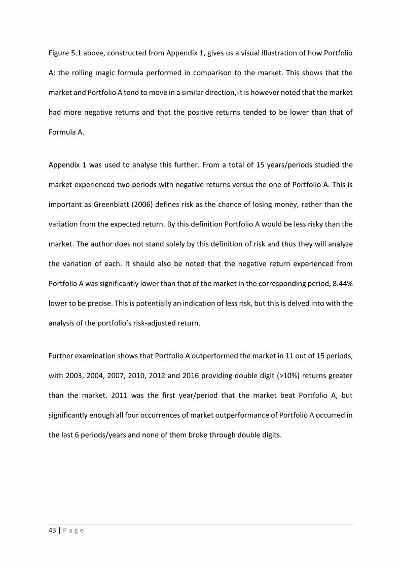
43 | P a g e

Figure 5.1 above, constructed from Appendix 1, gives us a visual illustration of how Portfolio

A: the rolling magic formula performed in comparison to the market. This shows that the

market and Portfolio A tend to move in a similar direction, it is however noted that the market

had more negative returns and that the positive returns tended to be lower than that of

Formula A.

Appendix 1 was used to analyse this further. From a total of 15 years/periods studied the

market experienced two periods with negative returns versus the one of Portfolio A. This is

important as Greenblatt (2006) defines risk as the chance of losing money, rather than the

variation from the expected return. By this definition Portfolio A would be less risky than the

market. The author does not stand solely by this definition of risk and thus they will analyze

the variation of each. It should also be noted that the negative return experienced from

Portfolio A was significantly lower than that of the market in the corresponding period, 8.44%

lower to be precise. This is potentially an indication of less risk, but this is delved into with the

analysis of the portfolio’s risk-adjusted return.

Further examination shows that Portfolio A outperformed the market in 11 out of 15 periods,

with 2003, 2004, 2007, 2010, 2012 and 2016 providing double digit (>10%) returns greater

than the market. 2011 was the first year/period that the market beat Portfolio A, but

significantly enough all four occurrences of market outperformance of Portfolio A occurred in

the last 6 periods/years and none of them broke through double digits.

44 | P a g e

Table 5.1: Key statistics of Portfolio A versus the Market

Table 5.1 above was derived from Appendix 1 and provides the annualized return, standard

deviation and Sharpe ratios for Portfolio A and the market over the full holding period. It also

provides a risk-adjusted return for Portfolio A.

The annualized return for Portfolio A is significantly higher at 19.46% for the holding period

than that of the market at 12.012%. Not only are the returns higher but it also produced a

standard deviation lower than that of the market, 0.1873 versus 0.1918 indicating it is less

volatile. This in conjunction with having less negative returns over the period shows that

Portfolio A is in fact less risky than the market. The author then analyzed the Sharpe Ratios

and noted that Portfolio A had a higher Sharpe ratio at 0.5742 than the market at 0.1726

indicating that Portfolio A produced greater excess returns per unit of volatility. Calculating a

risk-adjusted return provides further evidence of lower risk with the return of Portfolio A

increasing to 19.622% or by 0.162%.

Figure 5.2: Cumulative returns Portfolio A versus the Market

45 | P a g e

Figure 5.2 provides a good illustration of how Portfolio A outperforms the market. Investing

R100 in each at time period one, Portfolio A would have produced R1 439.16 by the end of

the holding period versus the R548.23 from the market.

Figure 5.3: Graphical representation of Portfolio B versus the Market

Figure 5.3 above, constructed from Appendix 2, gives one a visual illustration of how Portfolio

B: The magic formula (stocks purchased at a point in time) performed in comparison to the

market. This shows that the market and Portfolio B tend to move in a similar direction, even

more so than that of Portfolio A and the market.

Using Appendix 2 one can analyse these findings. As was the case with Portfolio A and the

market, from a total of 15 years/periods studied the market experienced more negative

returns than Portfolio B. In this case the market experienced three periods of negative yields

versus the one of Portfolio B. This is again significant by Greenblatt’s definition of risk. Again,

it is noted that the negative return experienced from Portfolio B was significantly lower than

that of the market in the corresponding period, 8.72% lower. While lower than the market it

was significantly higher than the only negative return in Portfolio A, roughly 8%. It is

46 | P a g e

interesting to note that for both Portfolio A and B the negative return occurred in 2009, the

peak of the financial crisis. While it looks as though the magic formula has provided superior

results so far, it was unable to protect investors from the crisis.

Further examination shows that Portfolio B outperformed the market in 11 out of 15 periods,

just like Portfolio A. With 2003, 2004, 2006, 2010, and 2012 providing double digit (>10%)

returns greater than the market, this is one less than Portfolio A. 2011 was the first

year/period that the market beat Portfolio B as was the case with Portfolio A, with all four

outperformances also occurring in the last 6 periods/years and none of them broke through

double digits.

Table 5.2: Key statistics of Portfolio B versus the Market

Table 5.2 above was derived from Appendix 2 and provides the annualized return, standard

deviation and Sharpe ratios for Portfolio B and the market over the full holding period. It also

provides a risk-adjusted return for Portfolio B.

The annualized return for Portfolio B is significantly higher at 19.361% for the holding period

than that of the market at 11.851%. Not only are the returns higher but it also produced a

standard deviation lower than that of the market all be it marginally, 0.2508 versus 0.2562

indicating it is marginally less volatile, making it slightly less risky. This in conjunction with

having less negative returns over the period shows that Portfolio B is in fact less risky than

the market. Upon analyzing the Sharpe ratios, it was noted that Portfolio B had a higher

Sharpe ratio at 0.4251 than the market at 0.1230 indicating that Portfolio B produced greater

47 | P a g e

excess returns per unit of volatility. Calculating a risk-adjusted return provides further

evidence of lower risk with the return of Portfolio A increasing to 19.508% or by 0.147%.

Figure 5.4: Cumulative returns Portfolio B versus the Market

Figure 5.4 provides a good illustration of how Portfolio B outperforms the market. Investing

R100 in each at the first period, Portfolio B would have produced R1 422.17 by the end of the

holding period versus the R536.50 from the market.

5.3 Portfolio A versus Portfolio B

Portfolio A and B consist of the same stocks, the fundamental difference between the two

portfolios is when stocks are bought and sold. Portfolio A is a purer form of the Greenblatt

magic formula as defined by Greenblatt himself, while Portfolio B is a slightly modified version

widely used in previous research.

The question becomes, does the timing of purchases affect the outcome or does the formula

identify value regardless?

48 | P a g e

Table 5.3: Key statistics of Portfolio A versus Portfolio B

The annual mean return of the two portfolios is very similar with Portfolio A producing 0.099%

greater return than Portfolio B. It is only when analyzing the risk coefficients, one noticed a

meaningful difference. Portfolio A has a considerably lower standard deviation at 0.1873 in

comparison to the 0.2508 of Portfolio B. This results in a risk-adjusted return of 19.622% for

Portfolio A and 19.508% for portfolio B. This increases the spread between the two to 0.114%,

which is marginally higher than the original 0.099%. It is also noted that the Sharpe ratio for

Portfolio A is higher at 0.5742 than that of Portfolio B at 0.4251, indicating that Portfolio A

produced greater excess returns per unit of volatility.

The above analysis has pointed out that the fundamental difference between the two

portfolios/methods of applying Greenblatts formula is risk. Staggered purchases of stocks

tended to lower the overall risk that the investor was exposed to, while still producing excess

returns.

While this report did not originally set out looking for the above it is a key finding none the

less and should be noted in research going forward.

49 | P a g e

5.4 The Magic Formula (Portfolio A and B) versus various other Market Indexes

Figure 5.5: Graphical representation of all annualized returns for indexes

Through inspection of figure 5.5 and the data pertaining to it we can state that most of the

indexes tend to move together 6. It is however noted, that over the period the two exceptions

to this (at least to some degree) would be the JSE Basic Minerals Index and the JSE Value

Indexes. The JSE Basic Minerals Index suffered six negative periods from a total of 15 and the

JSE Value Index amassed five. The next highest was three, why this is the case is outside the

scope of this report.

Table 5.4 in Appendix 3 allows one to analyze the various statistics relevant to the different

indexes and portfolios such as, the annualized returns, standard deviation, and the Sharpe

ratio.

6 The market will not be included in comparisons in this section as it was already compared to the magic formula in section 5.2.

50 | P a g e

From this analysis one can see that the annualized return from the magic formula: Portfolio

A and B are significantly higher than any of the index including the market as previously

stated. The best performing index was the JSE Small Cap with an annualized return of 14.74%,

which is 4.72% lower than Portfolio A and 4.62% lower than Portfolio B. The JSE Equally

Weighted Top 40 produced the next best return with 13.23%.

It is interesting to note that all indexes had at least two periods with negative returns with

the majority having three or more, unlike the magic formula which only had one in Portfolio

A and B respectively. Which again according to Greenblatt’s definition of risk makes Portfolio

A and B less risky than the market and all the indexes they are compared with in this study.

Moving one’s attention to the standard deviation of each portfolio/index one can again notice

that Portfolio A is substantially lower than all the others at 0.1873, the next best being the JSE

Equally Weighted Top 40 at 0.2428. Portfolio B coming in third with 0.2508 and the rest being

marginally higher than the last.

The Sharpe ratios tell the same story noted throughout the report, Portfolio A will produce

the greatest excess returns per unit of volatility with a Sharpe ratio of 0.5742, followed by

Portfolio B with a Sharpe ratio of 0.4251. The JSE Small cap would come in third at 0.2282 and

the JSE Equally Weighted Top 40 fourth at 0.1865.

51 | P a g e

Figure 5.6: Cumulative returns for Portfolio A, B, and the various indexes

Figure 5.6 provides an illustration of the cumulative returns that would have been earned

from each Portfolio or Index listed in Table 5.9. The assumption is that R100 was invested on

day one in each of the Portfolios. As can be seen Portfolio A and B would have accumulated

the most by a significant margin, each ending above R1420. The JSE Small cap would be third

amassing R786, fourth would be the JSE Equally Weighted Top 40 at R761.The JSE Growth

coming in R50 above the market. Only the JSE Value and JSE Basic Materials performing worse

than the market.

These finding are important because they show that in South Africa it is possible to

outperform the market on a consistent basis. It shows us that even if the Top 40 were used

as the market the magic formula would still have outperformed it. It also gives one an

indication that other investing strategies might also have outperformed the market, such as

a growth strategy or investing in a small stocks portfolio.

52 | P a g e

5.5 The Magic Formula versus alternative value investing portfolios

The alternative value portfolios were derived using key financial ratios that are commonly

used to signal value in a company namely, ROA, ROE and EY. The three ratios were selected

because Greenblatt himself refers to them and the need to modify them for superior gains.

These portfolios were constructed in a similar manner to that of Portfolio B, where by the top

30 stocks for each year were identified, purchased on day one of the trading period and sold

exactly one year after they were purchased. It is for this reason that all comparisons in this

section will only make use of Portfolio B and exclude Portfolio A.

Figure 5.7: Graphical representation of all annualized returns for alternative portfolios

Examination of figure 5.7 gives us a visual comparison of the yearly returns earned by each

of the portfolios against the market. The author noticed a similar trend to previous

comparisons; the portfolio returns tend to move in the same direction. It is however

interesting to note, that in 2003, 2004, 2009, 2010 and 2012 all portfolios had returns

53 | P a g e

greater than the market. 2011 and 2014 saw every portfolio underperform the market.

2003, 2005 and 2012 were marked by the biggest variations in returns between portfolios.

Table 5.5: Key statistics for the alternative portfolios, Portfolio B and the market

Using Table 5.5 derived from Appendix 4 one can analyze the performance of each portfolio

against the market and the magic formula. Through this analysis one can see that all the

portfolios produced annualized returns far greater than that of the market over the 15

periods/years. Even the worst performing portfolio (ROE) netted 2.25% more than the market

on an annualized basis. The ROA portfolio produced the greatest return at 19.86%, this was

0.5% higher than the magic formula return.

Turning our attention to the standard deviation, little variation between the portfolios is

noted. The ROE portfolio was the least volatile with a standard deviation of 0.2289 and EY

being the most volatile at 0.2626. This information is misleading to an extent, upon closer

examination of Appendix 4 one can see that the ROE portfolio had 5 negative periods, all be

it smaller ones. The magic formula again performed best in terms of having less negative

periods with just one, with the ROA portfolio suffering two and the EY portfolio and the

market suffering three.

The Sharpe ratio is again used to determine which portfolio produces the most excess returns

per unit of volatility. The ROA portfolio comes out on top here, followed closely by the magic

formula and some way behind in third is the EY portfolio.

54 | P a g e

To properly account for risk, a risk-adjusted return was calculated for each portfolio

mentioned above. This resulted in increased returns for three of the four portfolios, with EY

being the only exception and this is explained by the higher than market standard deviation

of the portfolio. The increases and one decrease however had no impact on their rankings.

Figure 5.8: Cumulative returns for alternative portfolios, Portfolio B and the market

Figure 5.8 provides the graphical illustration of the cumulative returns that would have been

earned from each Portfolio listed in Table 5.5 above. The assumption remains the same, invest

R100 on day one in each of the portfolios. The ROA Portfolio would have amassed slightly

above R1500, the magic formula would have come second with marginally over R1400, the

EY portfolio third with just under R1100, the ROE portfolio fourth with R720 and last would

be the market with R536.

55 | P a g e

CHAPTER 6

CONCLUSION

6.1 Conclusion

This report set out to back test Joel Greenblatt’s magic formula in South Africa and other value

investing strategies to determine if it was possible to systematically beat the market. This

report constructed both a rolling and static magic formula Portfolio and used the JSE All Share

Index as the market. The findings from this report were interesting and could add value to

future discussion regarding market efficiency.

Both magic formula portfolios managed to significantly outperform the market over the 15

years under investigation. What was interesting was that the ROA portfolio produced the

greatest return over the period and that all four value investing strategies outperformed the

market. It was interesting to see that even by testing other market indices the magic formula

still outperformed them. While this outperformance was there, it is noted that the market

started to outperform the magic formula in the latter years of the study. It is interesting to

note that the rolling portfolio outperformed the static portfolio over the same time period.

Not only did they outperform the market, but they had significantly lower risk. Not only was

risk lower by conventional measures but also by the definition outlined by Greenblatt. The

magic formula only produced one negative return during the period, which coincided with

the biggest financial crisis in a century. All other index or value strategies had at least two

negative years over the 15-year period. The higher Sharpe ratios of the value investing

portfolios shows us that these portfolios earned higher returns without taking on additional

risks.

56 | P a g e

Greenblatt’s formula makes use of data from previous years’ annual financial data and hence

would be available to everyone, the fact that this formula outperformed the market indicates

to us that the JSE in South Africa is not operating efficiently. This is further substantiated

through the outperformance of the other value investing strategies against the market.

6.2 Further Research

It was stated earlier that the rolling portfolio performed better and had a lower risk profile

than that of the static portfolio. This study bought shares over a period of five months, in

other words six shares per month. It would be interesting to see if rolling over differing

periods would make a difference on risk and reward. In other words, buy six shares every two

months or be more extreme and try two to four shares every month.

It is suggested that in 5 years this study be performed again bringing the years under study

forward. This would be in the hopes of discovering why the market started to outperform the

magic formula in later years. It could be an indication that the South African market was/is

maturing and becoming efficient.

The final recommendation is for a student to perform factor analysis and determine if there

are any other variables that could add value to the magic formula by lowering risk, increasing

returns or both.

57 | P a g e

References

Ball, R., Kothari, S. P., & Shanken, J. (1995). Problems in Measuring Portfolio Performance, an

Application to Contrarian Investment Strategies. Journal of Financial Economics, 38(1),

79-107.

Banz, R. W. (1981). The relationship between return and market value of common stocks.

Journal of Financial Economics, 9, 3-18.

Basu, S. (1977). Investment Performance of Common Stocks in Relations to Their Price-

Earnings Ratios: A Test of the Efficient Market Hypothesis. The Journal of Finance,

32(3), 663-682.

Baytas, A., & Cakici, N. (1999). Do Markets Overreact: International Evidence. Journal of

Banking & Finance, 23, 1121-1144.

Beunza, D., & Stark, D. (2004). Tools of the trade: the socio-technology of arbitrage in a Wall

Street trading room. Industrial and Corporate Change, 13(2), 369 - 400.

Brown, P., Kleidon, A., & Marsh, T. (1983). New evidence on the nature of size-related

anomalies in stock prices. Journal of Financial Economics, 12, 13-32.

Campbell, J. Y., & Shiller, R. J. (1998). Valuation ratios and the long-run stock market outlook.

Journal of Portfolio Management, 24, 11-26.

Capaul, C., Rowley, I., & Sharpe, W. F. (1993). International value and growth stock returns.

Financial Analysts Journal, 49(1), 27-36.

Chahine, S. (2008). The Effects of Information Disclosure and Board Independence on IPO

Discount. Journal of Small Business Management, 46(2), 159-311.

Chan, K. C., & Chen, N.F. (1991). Structural and return characteristics of small and large firms.

Journal of Finance, 46, 1467-1484.

Chan, K. C., Hamao, Y., & Lakonishok, J. (1991). Fundamentals and stock returns in Japan.

Journal of Finance, 46, 1739-1764.

Clarke, J., Jandik, T., & Mandelker, G. (2001). The Efficient Market Hypothesis – An Overview,

in R. C. Arffa (Leading Financial Experts: Investment Strategies from Industry Leaders

ed.). New York: Wiley.

Conrad, J., & Kaul, G. (1993). Long-term market overreaction or biases on computed returns?

Journal of Finance, 48(1), 39-63.

58 | P a g e

Coval, J. D., Hirshleifer, D., & Shumway, T. (2005). Can Individual Investors Beat the Market?

Retrieved 22nd February, 2018, from

http://www.people.hbs.edu/jcoval/Papers/persist.pdf

Cross, F. (1973). The behaviour of stock prices on Friday and Mondays. Financial Analysts

Journal, 29(6), 67-69.

Dao, P. (2016). Performance evaluation based on financial ratios. Thesis, Arcada University, Helsinki

Daniel, G., Sornette, D., & Wohrmann, P. (2009). Look-Ahead Benchmark Bias in Portfolio

Performance Evaluation. Journal of Portfolio Management, 36(1), 121-130.

De Bondt, W. F., & Thaler, R. H. (1985). Does the stock market overreact? Journal of Finance,

40(3), 793-805.

Degutis, A., & Novickytė, L. (2014). THE EFFICIENT MARKET HYPOTHESIS: A CRITICAL REVIEW

OF LITERATURE AND METHODOLOGY. EKONOMIKA, 93 (2), 7 - 23.

De Moor, L., Van den Bossche, F., & Verheyden, T. (2013). A Tale of Market Efficiency. Review

of Economic and Business Literature, 58(2), 139-156.

Dhatt, M. S., Kim, Y. H., & Mukherji, S. (1999). The Value Premium for Small Capitalization

Stocks. Financial Analysts Journal, 55(5), 60-68.

Fama, E. (1965). The behaviour of stock market prices. Journal of Business, 38, 34-105.

Fama, E. F. (1970). Efficient Capital Markets: A Review of Theory and Empirical Work. The

Journal of Finance, 25 (2), 383 – 417.

Fama, E., & French, K. R. (1992). The Cross-Section of Expected Stock Returns. The Journal of

Finance, 47(2), 427-465.

Fama , E., & French , K. R. (1993). Common risk factors in the returns on stocks and bonds.

Journal of financial economics, 33(1), 3-56.

Fama , E., & French , K. R. (1998). Value versus growth: The international evidence. Journal of

Finance, 53(6), 1975-1999.

Fama , E., & French , K. R. (2001). Disappearing Dividends: Chaning Firm Characteristics or

Lower Propensity to Pay. Journal of Financial Economics, 60(1), 3-43.

Fama, E., & French , K. R. (2012). Size, value, and momentum in international stock returns.

Journal of Financial Economics, 105, 457-472.

Fluck, Z., Malkiel, B., & Quandt, R. E. (1997). The Predictability of Stock Returns: A Cross-

Sectional Simulation. Review of Economics and Statistics, 79(2), 176-183.

59 | P a g e

French , K. R. (1980). Stock returns and the weekend effect. Journal of Financial Economics, 8,

55-70.

Frankel, M. (2010). How Peter Lynch Destroyed the Market. Retrieved 22 February, 2018,

from https://www.fool.com/investing/general/2010/05/21/how-peter-lynch-

destroyed-the-market.aspx

Frankel, M. (2017). Warren Buffet has been crushing the stock market since 1965 - here's how

he's done it. Retrieved 22 February, 2018, from

http://www.businessinsider.com/how-much-has-warren-buffett-beaten-the-market-

by-2017-3

Fu, S., & Xia, C. (2016). Does Magic Formula Investing Work in Hong Kong Stock Market?

Master’s thesis, The University of Hong Kong, Hong Kong.

Gibson, G. (1889). The Stock Markets of London, Paris and New York. New York: G.P. Putnam’s

Sons.

Giudici, P. (2003). Applied Data Mining Statistical Methods for Business and Industry.

Chichester: John Wiley & Sons Ltd.

Greenblatt, J. (2006). The little book that beats the market. . Hoboken, New Jersey: John Wiley

& Sons, Inc.

Guo, S., & Wang, Z. (2007). Market efficiency anomalies. A study of seasonality effect on the

Chinese stock exchange. Master’s thesis, Umeå School of Business, Sweden.

Hämäläinen, J. (2007). MOMENTUM AND CONTRARIAN INVESTMENT STRATEGIES. Thesis,

Lappeenranta University of Technology School of Business, Finland.

Haugen, R. A. (1995). The new finance: The case against efficient market. New Jersey: Prentice

Hall.

Herrera, M. J., & Lockwood, L. J. (1994). The Size Effect in the Mexican Stock Market. Journal

of Banking and Finance, 18 (1), 612-632.

Ho, Y. K. (1990). Stock Return Seasonalities in Asia Pacific Markets. Journal of International

Financial Management & Accounting, 2(1), 47-77.

Horowitz, J. L., Loughran, T., & Savin, N. E. (2000). The Disappearing Size Effect. Research in

Economics, 54, 83-100.

Howard, W. F. (2015). An investment strategy based on return on capital and earnings yield.

Master’s thesis, Stellenbosch University, Stellenbosch.

Jaffe, J., Keim, D. B., & Westerfield, R. (1989). Earnings Yields, Market Values, and Stock

Returns. The Journal of Finance, 44(1), 135-148.

60 | P a g e

Jegadeesh, N., & Titman, S. (1993). Returns to Buying Winners and Selling Losers Implications

for Stock Market Efficiency. Journal of Finance, 47(1), 65-90.

Jordan, B., Miller, T., & Dolvin, S. (2015). Fundamentals of investments: Valuation and

management (7 ed.). New York: McGraw-Hill Education.

Keim, D. B. (1983). Size-Related Anomalies and Stock Return Seasonality: Further Empirical

Evidence. Journal of Financial Economics, 12, 13-21.

Keim, D. B., & Stambaugh, R. F. (1984). A further investigation of the weekend effect in stock

returns. Journal of Finance, 39(3), 819-835.

Klein, R. W., & Bawa, V. S. (1977). The effect of limited information and estimation risk on

optimal portfolio diversification. Journal of Financial Economics, 5, 89-111.

Kryzanowski, L., & Zhang, H. (1992). The Contrarian Investment Strategy Does Not Work in

Canadian Markets. Journal of Financial and Quantitative Analysis, 27(3), 383-395.

Lakonishok, J., Schleifer, A., & Vishny, R. W. (1994). The Contrarian Investment, Extrapolation,

and Risk. The Journal of Finance, 49(5), 1541-1578.

Larkin, P. J. (2009). Can individual investors capture the value premium. Journal of Business

and Economics Research, 7(5), 25-34.

Levy, R. (1967). Relative Strength as a Criterion for Investment Selection. Journal of Finance,

22, 595–610.

Mabhunu, M. (2004). THE MARKET EFFICIENCY HYPTOTHESIS AND THE BEHAVIOUR OF STOCK

RETURNS ON THE JSE SECURITIES EXCHANGE. Master’s thesis, Rhodes University,

Grahamastown.

Malkiel, B. G. (1973). A Random Walk Down Wall Street, Norton, New York.

Malkiel, B. (2003). The Efficient Market Hypothesis and Its Critics. The Journal of Economic

Perspectives, 17(1), 59-82.

Malkiel, B. G. (2011). The Efficient-Market Hypothesis and the Financial Crisis Retrieved 11

November, 2016, from http://www.russellsage.org/sites/all/files/Rethinking-

Finance/Malkiel.%20The%20Efficient-

Market%20Hypothesis%20and%20the%20Financial%20Crisis%20102611.pdf .

Miller, E. M. (1988). Why a weekend effect? Individuals are net sellers on balance and do

more selling on Mondays than on other days. Journal of Portfolio Management, 14(4),

43-48.

61 | P a g e

Moskowitz, T. J., & Grinblatt, M. (1999). Do Industries Explain Momentum? Journal of Finance,

54(4), 1249–1290.

Njanike, E. (2010). IS THE SOUTH AFRICAN STOCK MARKET EFFICIENT? MEAN REVERSION ON

THE JSE. Master’s thesis, University of Cape Town, Cape Town.

Olin, T. (2011). Value investing in the Finnish stock market. Master’s thesis, Aalto University,

Finland

Oppenheimer, H. R. (1986). Ben Graham's net current asset values: A performance update.

Financial Analysts Journal, 42(6), 40-127.

Pawley, M. G. (2006). The impact of survivorship bias on South African unit trust. Investment

Analysts Journal, 64, 21-26.

Persson, E., & Stahlberg, C. (2006). P/E and EV/EBITDA Investment Strategies vs. the Market.

Master’s thesis, Linkoping University, Sweden.

Persson, V., & Selander N. (2009). Back testing “The Magic Formula” in the Nordic region.

Master’s thesis, Stockholm School of Economics, Sweden

Postma, P. P. M. (2015). Magic Formula investing in the Benelux. Thesis, Tilburg University,

Netherland

Reinganum, M. R. (1981). Misspecification of capital asset pricing: Empirical anomalies based

on earnings' yields and market values. Journal of Financial Economics, 9, 19-46.

Roll, R. (1983). The-turn-of-the-year effect and the return premia of small firms. Journal of

Portfolio management, 9, 18-28.

Rouwenhorst, G. K. (1998). International Momentum Strategies. Journal of Finance, 53(1),

267–284.

Rozeff, M. S., & Kinney, W. R. (1976). Capital market seasonality: The case of stock returns.

Journal of Financial Economics, 3(4), 379-402.

Rubenstein, M. (2001). Rational Markets: Yes or no? The affirmative case. Financial Analysts

Journal, 57(3), 15-29.

Sewell, M. (2011). History of the Efficient Market Hypothesis. Research Note, London.

Shiller, R. J. (2003). From Efficient Markets Theory to Behavioral Finance. The Journal of

Economic Perspectives, 17(1), 83-104.

Stattman, D. (1980). Book values and stock returns. The Chicago MBA: A Journal of Selected

Papers, 4, 25-45.

Thaler, R. H. (1987). The January effect. The Journal of Economic perspectives, 1(1), 197-201.

62 | P a g e

Titman, S., & Daniel , K. (1997). Evidence on the characteristics of cross-sectional variation in

stock returns. Journal of Finance, 52(1), 113-173.

Yavrumyan, E. (2015). Efficient Market Hypothesis and Calendar Effects: Evidence from the

Oslo Stock Exchange. Master’s thesis, University of Oslo, Oslo.

Ziemba, W. T. (1991). The Role of Beta and Size in the Crosssection of European Stock Returns.

Japan and the World Economy, 3 (1), 119-146.

63 | P a g e

Appendix 1:

Table A: Portfolio A Results versus the Market

Portfolio: A All Share: A MF – All Share

2002 20.99% 19.14% 1.85%

2003 10.22% -20.28% 30.50%

2004 43.32% 22.95% 20.37%

2005 34.22% 31.61% 2.61%

2006 49.34% 47.28% 2.05%

2007 49.62% 33.31% 16.31%

2008 6.05% 5.60% 0.46%

2009 -16.95% -25.39% 8.44%

2010 36.79% 22.02% 14.77%

2011 8.99% 16.87% -7.88%

2012 20.57% 6.28% 14.28%

2013 14.85% 17.70% -2.85%

2014 16.87% 22.03% -5.15%

2015 1.91% 4.40% -2.49%

2016 15.94% 1.46% 14.48%

Mean 19.46%

12.012% 7.448%

64 | P a g e

Appendix 2:

Table B: Portfolio B Results versus the Market

Portfolio: B All Share: B MF – All Share

2002 28.18% 23.73% 4.45%

2003 7.67% -30.23% 37.90%

2004 59.57% 42.37% 17.20%

2005 28.40% 28.05% 0.36%

2006 74.59% 62.09% 12.50%

2007 31.67% 29.01% 2.66%

2008 7.87% 5.03% 2.84%

2009 -25.04% -33.76% 8.72%

2010 50.66% 39.23% 11.43%

2011 6.34% 12.46% -6.12%

2012 15.65% 2.19% 13.46%

2013 14.80% 15.88% -1.07%

2014 18.16% 23.33% -5.16%

2015 4.41% 6.78% -2.37%

2016 3.10% -4.02% 7.12%

Mean 19.361% 11.851% 7.51%

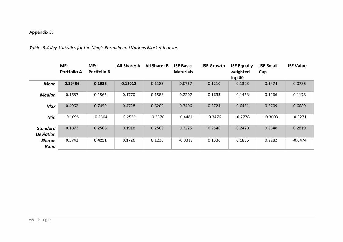
65 | P a g e

Appendix 3:

Table: 5.4 Key Statistics for the Magic Formula and Various Market Indexes

MF: Portfolio A

MF: Portfolio B

All Share: A

All Share: B

JSE Basic Materials

JSE Growth

JSE Equally weighted top 40

JSE Small Cap

JSE Value

Mean 0.19456

0.1936 0.12012

0.1185 0.0767 0.1210 0.1323 0.1474 0.0736

Median 0.1687

0.1565 0.1770

0.1588 0.2207 0.1633 0.1453 0.1166 0.1178

Max 0.4962

0.7459 0.4728

0.6209 0.7406 0.5724 0.6451 0.6709 0.6689

Min -0.1695

-0.2504 -0.2539

-0.3376 -0.4481 -0.3476 -0.2778 -0.3003 -0.3271

Standard Deviation

0.1873

0.2508 0.1918

0.2562 0.3225 0.2546 0.2428 0.2648 0.2819

Sharpe Ratio

0.5742

0.4251 0.1726

0.1230 -0.0319

0.1336 0.1865 0.2282

-0.0474

66 | P a g e

Appendix 4:

Table C: Alternative investment strategies

ROA ROE EY Portfolio B All Share

2002 13.45% -0.82% 19.23% 28.18% 23.73%

2003 13.24% -7.95% -1.41% 7.67% -30.23%

2004 56.59% 49.10% 59.33% 59.57% 42.37%

2005 48.26% 27.77% 49.80% 28.40% 28.05%

2006 74.22% 64.04% 56.44% 74.59% 62.09%

2007 35.27% 21.75% 30.70% 31.67% 29.01%

2008 3.51% -4.10% 4.14% 7.87% 5.03%

2009 -19.55% -19.30% -28.84% -25.04% -33.76%

2010 43.37% 43.35% 59.42% 50.66% 39.23%

2011 9.39% 11.36% 7.58% 6.34% 12.46%

2012 16.99% 17.25% 16.13% 15.65% 2.19%

2013 17.08% 21.02% 12.68% 14.80% 15.88%

2014 14.08% 12.84% 16.12% 18.16% 23.33%

2015 10.37% 9.85% 4.80% 4.41% 6.78%

2016 -4.34% -4.24% -5.64% 3.10% -4.02%

Mean 19.86% 14.10% 17.30% 19.361% 11.851%

Std Dev 0.2473 0.2289 0.2626 0.2508 0.2562

Sharpe Ratio 0.4513 0.2357 0.3276 0.4251 0.1230

Risk-Adjusted Return

20.114%

14.26%

17.18%

19.51%