Analysing the dependencies of cross-shore evolution of ... · Analysing the dependencies of...

Analysing the dependencies of cross-shore

evolution of near-bed orbital velocity on

physical parameters

Yulai Wang

MSc. Thesis

Water Engineering & Management

University of Twente

The Netherlands

September 2016

Supervision committee:

Head supervisor: Dr. Ir. Jan S. Ribberink


Daily supervisor: Dr. Ir. Angels Fernandez-Mora


External supervisor: Dr. Ir. Jebbe van der Werf

University of Twente, Deltare

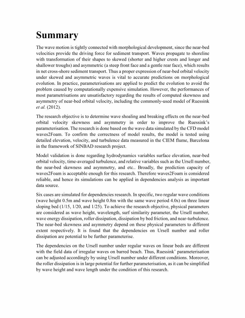
Summary The wave motion is tightly connected with morphological development, since the near-bed

velocities provide the driving force for sediment transport. Waves propagate to shoreline

with transformation of their shapes to skewed (shorter and higher crests and longer and

shallower troughs) and asymmetric (a steep front face and a gentle rear face), which results

in net cross-shore sediment transport. Thus a proper expression of near-bed orbital velocity

under skewed and asymmetric waves is vital to accurate predictions on morphological

evolution. In practice, parameterisations are applied to predict the evolution to avoid the

problem caused by computationally expensive simulation. However, the performances of

most parametrisations are unsatisfactory regarding the results of computed skewness and

asymmetry of near-bed orbital velocity, including the commonly-used model of Ruessink

et al. (2012).

The research objective is to determine wave shoaling and breaking effects on the near-bed

orbital velocity skewness and asymmetry in order to improve the Ruessink’s

parameterisation. The research is done based on the wave data simulated by the CFD model

waves2Foam. To confirm the correctness of model results, the model is tested using

detailed elevation, velocity, and turbulence data measured in the CIEM flume, Barcelona

in the framework of SINBAD research project.

Model validation is done regarding hydrodynamics variables surface elevation, near-bed

orbital velocity, time-averaged turbulence, and relative variables such as the Ursell number,

the near-bed skewness and asymmetry, and etc.. Broadly, the prediction capacity of

waves2Foam is acceptable enough for this research. Therefore waves2Foam is considered

reliable, and hence its simulations can be applied in dependencies analysis as important

data source.

Six cases are simulated for dependencies research. In specific, two regular wave conditions

(wave height 0.5m and wave height 0.8m with the same wave period 4.0s) on three linear

sloping bed (1/15, 1/20, and 1/25). To achieve the research objective, physical parameters

are considered as wave height, wavelength, surf similarity parameter, the Ursell number,

wave energy dissipation, roller dissipation, dissipation by bed friction, and near-turbulence.

The near-bed skewness and asymmetry depend on these physical parameters to different

extent respectively. It is found that the dependencies on Ursell number and roller

dissipation are potential to be further parameterise.

The dependencies on the Ursell number under regular waves on linear beds are different

with the field data of irregular waves on barred beach. Thus, Ruessink’ parameterisation

can be adjusted accordingly by using Ursell number under different conditions. Moreover,

the roller dissipation is in large potential for further parameterisation, as it can be simplified

by wave height and wave length under the condition of this research.

Contents

1.Introduction ...................................................................................................................... 1

1.1 Research background .................................................................................................1

1.2 Research objective and questions ..............................................................................3

1.3 Research tools ............................................................................................................4

1.3.1 waves2Foam .................................................................................................. 4

1.3.2 MATLAB ....................................................................................................... 4

1.4 Research approaches and outlines .............................................................................4

2.Methodology .................................................................................................................... 7

2.1 SINBAD mobile bed experiment ...............................................................................7

2.1.1 Experiment set-up .......................................................................................... 7

2.1.2 Measurements ................................................................................................ 7

2.2 Model simulations ......................................................................................................9

2.2.1 SINBAD simulation ....................................................................................... 9

2.2.2 Designed cases ............................................................................................... 9

2.3 Physical parameters .................................................................................................11

2.4.1 Basic wave parameters ................................................................................. 11

2.4.2 Ursell number............................................................................................... 11

2.4.3 Surf similarity .............................................................................................. 11

2.4.4 Energy dissipation ........................................................................................ 11

2.4.5 Turbulence ................................................................................................... 12

2.4 Fitting methods ........................................................................................................13

3.Model validation ............................................................................................................ 15

3.1 Hydrodynamics equilibrium ....................................................................................15

3.2 Surface elevation ......................................................................................................18

3.3 Near-bed orbital velocity .........................................................................................21

3.4 Turbulence ...............................................................................................................24

3.4 Conclusion ...............................................................................................................25

4.Dependencies analysis ................................................................................................... 27

4.1 Hydrodynamics equilibrium ....................................................................................27

4.2 Wave height .............................................................................................................28

4.3 Wavelength ..............................................................................................................29

4.4 Ursell number ...........................................................................................................31

4.5 Surf similarity parameter .........................................................................................33

4.6 Energy dissipation ....................................................................................................34

4.6.1 Wave energy dissipation .............................................................................. 34

4.6.2 Roller dissipation ......................................................................................... 35

4.6.3 Dissipation due to bed friction ..................................................................... 36

4.7 Near-bed turbulence .................................................................................................37

4.8 Conclusion ...............................................................................................................38

5.Discussion ...................................................................................................................... 41

6.Conclusion and recommendations ................................................................................. 45

6.1 Conclusion ...............................................................................................................45

6.2 Recommendations ....................................................................................................47

References ......................................................................................................................... 49

List of symbols .................................................................................................................. 51

List of Figures ................................................................................................................... 53

List of Tables .................................................................................................................... 57

Appendix ........................................................................................................................... 59

A.Depth-averaged turbulence ........................................................................................... 59

B.Data extraction and treatment ....................................................................................... 65

B.1 Data extraction ........................................................................................................65

B.2 Data treatment .........................................................................................................66

B.2.1 Averaging .................................................................................................... 66

B.2.2 Near-bed orbital velocity ............................................................................. 66

B.2.3 Experimental turbulence ............................................................................. 66

C.Ruessink-Abreu parameterisation ................................................................................. 69

1

Chapter 1

Introduction

1.1 Research background

The orbital motion of the water particles of waves change from purely circular in the deep

sea to increasingly elongated ellipse in shallow water. Consequently, the near-bed orbital

motion is unavoidably influenced. Specifically, its oscillation over time is sinusoidal in the

deep sea, while becomes irregular when waves gradually approach the coastline. The non-

linearity can be categorised as skewness and asymmetry. A skewed wave has higher and

shorter crest, and shallower and longer trough. Moreover, an asymmetric wave behaves as

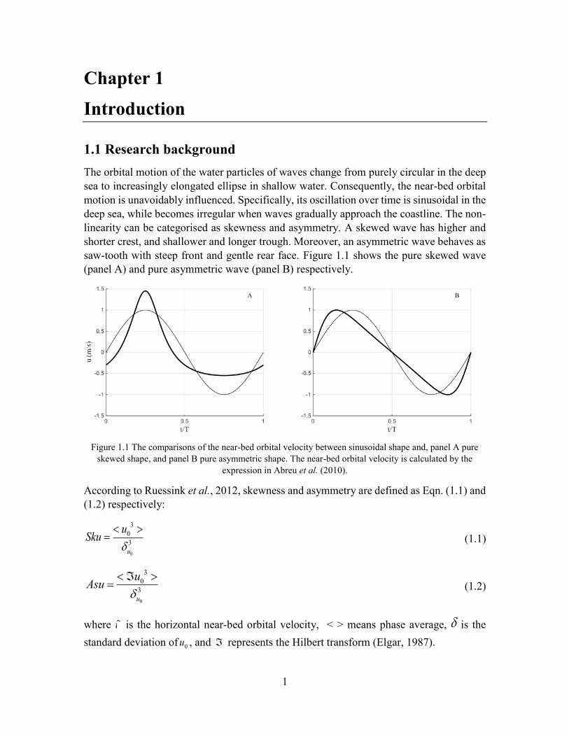
saw-tooth with steep front and gentle rear face. Figure 1.1 shows the pure skewed wave

(panel A) and pure asymmetric wave (panel B) respectively.

Figure 1.1 The comparisons of the near-bed orbital velocity between sinusoidal shape and, panel A pure

skewed shape, and panel B pure asymmetric shape. The near-bed orbital velocity is calculated by the

expression in Abreu et al. (2010).

According to Ruessink et al., 2012, skewness and asymmetry are defined as Eqn. (1.1) and

(1.2) respectively:

0

3

0

3

u

uSku

(1.1)

0

3

0

3

u

uAsu

(1.2)

where 0u is the horizontal near-bed orbital velocity, < > means phase average, is the

standard deviation of 0u , and represents the Hilbert transform (Elgar, 1987).

2

Being an essential driving factor to morphological development, the motion of near-bed

water particles is highly relevant to coastal and nearshore engineering. Also, it was proved

that skewed and asymmetric wave results in onshore bar migration (Elgar et al., 2001,

Ruessink et al., 2011). Therefore a proper expression of the cross-shore near-bed orbital

motion is essential to morphodynamics prediction. Accurate prediction in terms of water

surface and outer fluxes can be presented by advanced wave models, like Reynolds-

Averaged Navier-Stokes models (e.g. Jacobsen et al., 2012), Boussinesq models (e.g.

Kennedy et al., 2010), Large eddy simulation (e.g. Christensen and Rolf, 2001), and Direct

numerical simulation (e.g. Kim et al., ). However, they are too computationally demanding

to be used for mid- and long-term morphodynamics simulations. Therefore, some

morphological models have implemented existing parameterization of near-bed orbital

velocity which drives sediment transport. These parameterizations have been developed to

predict the orbital velocity shape using relatively simple analytical expressions. Using

water depth, (deep-water) wave height, wavelength, and bed slope, Isobe and Horikawa

(1982) parameterized both skewned and asymmetric near-bed velocity for regular waves

at normal incidence. Elfrink et al. (2006) derived a different piecewise function of near-

bed velocity for irregular shoaling waves at normal incidence based on a large amount of

field data. However, both functional forms of Isobe and Horikawa (1982) and Elfrink et al.

(2006) are discontinuous regarding velocity and corresponding acceleration (Abreu et al.

2010; Malarkey and Davies 2012).

Based on the work of Drake and Calantoni. (2001), Abreu et al. (2010) derived a

parameterization of near-bed velocity which calculates continuous regular time series

which are approximation of Isobe and Horikawa (1982) and Elfrink et al. (2006). However,

Abreu et al. (2010) work is cumbersome and requires solving cubic equations (Malarkey

and Davies, 2012). Ruessink et al., (2012) characterised a simpler parameterization of

skewness and asymmetry, which can be applied in the analytical expression of near-bottom

velocity of Abreu et al., (2010) to simulate velocity time series.

Van den Broek (2015) used data from SINBAD fixed bed experiment (Van der A. et al. to

be submitted) to test three parameterizations of Isobe and Horikawa (1982), Elfrink et al.

(2006), Ruessink et al. (2012) (hereafter referred as Ruessink parameterization. Ruessink

parameterisation better predicted in velocity peaks and troughs, and skewness than the

other two methods. However, the deviations of Ruessink parameterisation predictions are

still inaccurate regarding underestimation of skewness and asymmetry. An improved

parameterisation is necessary for sand transport models when an accurate prediction is

required, especially in the breaking zone (Van den Broek, 2015).

Two reasons could explain this mismatch between Ruessink’s method and the experimental

data. One is that Ruessink et al., (2012) calibrated their parameterisation with irregular

waves from field observation, while Van den Broek (2015) used regular and unidirectional

wave data in experiment. Consequently, “Ruessink parameterisation may underestimate

skewness of orbital velocity in laboratory wave” (Ruessink et al., 2012), since irregular

waves do not break intensively while regular waves do. The other is that the most vital

3

input of Ruessink parameterisation is defined by the Ursell number which is calculated

according to linear wave theory. However, wave shoaling and breaking are non-linear

processes due to wave deformation, which may cause the mismatch of Ruessink

parameterisation.

Although Ruessink parameterisation defects are noticeable, it has the large potential to be

further improved because it is simply computed, is able to predict pronounced bar

migration, and can be applied in Abreu’s expression to generate continuous wave series.

Besides the Ursell number, some other physical processes (introduced in the section 1.3 in

this chapter) are hypothesized to relate the near-bed orbital velocity skewness and

asymmetry. These physical processes, as well as the Ursell number, are going to be

analysed in order to improve the prediction capacity of Ruessink parameterisation.

1.2 Research objective and questions

Based on the drawbacks of Ruessink parameterisation prediction, the research objective is:

To determine wave shoaling and breaking effects on the near-bed orbital velocity skewness

and asymmetry in order to improve the parameterisation by Ruessink et al. (2012).

As parameterisation is derived from large amount of data, in this research model

waves2Foam (described in the next section) is used as wave data generator. Simulated data

is going to be studied in order to achieve the research objective. Therefore three research

questions are formulated as:

1. How well can wave2Foam simulate near-bed orbital velocity under regular waves?

1.1 What experimental data is available for model validation?

1.2 Can waves2Foam satisfactory predict surface elevation, cross-shore elevation

profiles, and the Ursell number?

1.3 Can waves2Foam satisfactorily predict near-bed orbital velocity, cross-shore

velocity profiles, skewness and asymmetry?

1.4 Can wave2Foam satisfactorily predict vertical time-averaged turbulence?

2. How do wave shoaling and breaking affect the near-bed orbital velocity?

2.1 Which physical parameters are associated to wave shoaling and breaking?

2.2 Do the near-bed skewness and asymmetry depend on these physical parameters?

2.3 How is these relations affected by bed slope and wave height?

3. How can the Ruessink parameterisation be improved?

3.1 Which physical parameters associated wave shoaling and breaking are potential for

parameterisations?

4

3.2 How can the effect of shoaling and breaking on near-bed orbital velocity be

parameterised under the condition of regular waves on linear beds?

1.3 Research tools

1.3.1 waves2Foam

The computational fluid dynamics (CFD) model waves2Foam (Jacobsen et al. 2012)

coupled with SediMorph (sediment transport model) is a wave generator which uses the

Reynolds-Averaged Navier-Stokes equations coupled with a volume of fluid method to

solve two-phase flow problems. For turbulence, modified k-ε and k-ω shear stress transport

models (Brown et al. 2014, 2016) are embedded. In this research, the simulated turbulence

data is based on k-ε model, because k-ε model is more reliable than the other according to

a test (personal communication with Fernandez-Mora A., June, 2016). The high resolution

is desired to simulate accurately wave motion, especially near-bed processes. Since the

spatial domains for all runs are different, the grids are accordingly unlike (introduced in

Chapter 2). The model outputs consist of velocity field (horizontal, vertical, and lateral),

water-air interface coefficient, sediment concentration, turbulence, turbulence dissipation,

eddy viscosity, and pressure. The outputs are stored in C++ ASCII files at each

computational point per time step.

1.3.2 MATLAB

MATLAB is mainly used in this research in terms of:

1. selecting the required data from whole data set. The required data is introduced in

Chapter 2, and the essential selecting methods are presented in Appendix B.

2. treating selected the selected data in needed formations for different usages. The

method of data treatment is given in Appendix B.

3. computing required physical parameters based on the treated data for model

validation and case studies respectively. The expressions of physical parameters are

shown in Chapter 2.

4. for case studies , analysing the dependencies of near-bed skewness and asymmetry

on physical parameters which is further fitted based on the method in the last

section in Chapter 2.

1.4 Research approaches and outlines

Ruessink et al. (2012) derived the parameterisation with the data on barred beaches with

water depth h between 0.25 and 11.2m, and irregular waves with significant wave height

Hs between 0.05 and 3.99m, and period T between 3.1 and 13.9s. This research focuses on

simpler cases, regular waves on linear beds, as the primary step to understand the

dependencies of near-bed skewness and asymmetry on wave shoaling and breaking. The

wave conditions are designed within the validity range of Ruessink’s method as wave

5

height H=0.5m and 0.8m with same period T=4.0s. Moreover the deep water depth is 2.55m.

The wave conditions and deep water depth are designed referring to SINBAD mobile bed

experiment in CIEM flume (introduced in Chapter 2). This research is a start of the analysis

of the dependencies of near-bed skewness and asymmetry on other physical parameters.

To simply the analysis, the linear sloping bed are considered. The bed slopes are chosen as

1/15, 1/20, and 1/25 to investigate the bed slope effects on the dependencies. Moreover,

this research as the extend study regarding bed slopes of Ruessink’ work, as Ruessink et

al. (2012) suggested the bed slope gentler than 1/30.

For the research question “1. How well can wave2Foam simulate near-bed orbital velocity

under regular waves?”, the experimental data (SINBAD mobile bed project) for model

validation, and the validation run of model are introduced in Chapter 2. Then Chapter 3

shows the results of model validation regarding surface elevation, near-bed orbital velocity

and turbulence themselves, and other variables based them, e.g. cross-shore profile of

surface elevation.

The research questions “2. How do wave shoaling and breaking affect the near-bed orbital

velocity?” and “3. How can the Ruessink parameterisation be improved?” are tightly

related, i.e., research question 3 is answered based on the findings in research question 2.

Chapter 2 introduces the simulated physical parameters which are associated to wave

shoaling and breaking. They are chosen from basic to complex as wave height, wave length,

surf similarity, the Ursell number, energy dissipation (wave energy dissipation, roller

dissipation, and dissipation due to bed friction), and near-bed turbulence. The dependencies

of near-bed skewness and asymmetry on the Ursell number is confirmed by Ruessink et al.

(2012) under irregular wave conditions on barred beaches, and is going to be analysed in

this research for regular waves. Surf similarity is chosen for investigating slope effects.

Furthermore, energy dissipation and near-bed turbulence are detailed physical processes,

and are hypothesized to relate to near-bed skewness and asymmetry. Chapter 4 presents

the dependencies analysis which is done by relating near-bed skewness and asymmetry as

functions of physical processes. And the physical parameters- which are clearly related to

relation to near-bed skewness and asymmetry are selected for further discussion in Chapter

5 where research question 3 is answered partly.

This thesis finally presents conclusions with answering the research questions and the

recommendations for further research.

7

Chapter 2

Methodology

The research methodology is described in this chapter. Section 2.1 introduces the available

experimental data (SINBAD mobile bed project) for model validation. Section 2.2 presents

the model simulations for validation and designed cases respectively. Then the calculations

of interesting physical parameters which are associated to wave shoaling and breaking are

shown in Section 2.3, while the fitting techniques are briefly introduced in Section 2.4. The

according data treatment, e.g. data selection, data averaging, is shown in Appendix B.

2.1 SINBAD mobile bed experiment

2.1.1 Experiment set-up

The experiment was done in the CIEM wave flume (at Universitat Politecnica de Catalunya

in Barcelona) with a length of 100m, a width of 3m and 4.5m depth. Figure 2.1 shows the

experimental set-up. The x-axis shows the cross-shore position in the flume where the

paddle was located at x=0m. Z-axis indicates the positons upwards in the flume where the

still water level (SWL) was set at z=0m. The foreslope was 1:10, and a breaker bar was

located between 50m and 58m. After the breaker bar was an 18m long and 1.35m deep

horizontal bed followed by a dissipative beach. Figure 2.1 bottom panel depicts the

shoaling region (x<55.5m), breaking region (55.5<x<59.0m), and inner surf zone where

roller develops (x>59.0m) (Van der Zanden et al. 2016). The breaking point was not fixed

and slowly shifted onshore due to morphological evolution. The wave paddle was located

at x=0m with 2.55m water depth. It generated regular waves with wave height H=0.85m

and wave period T=4.0s. Firstly the initial bed developed for 105 minutes. Then the

reference bed profile (Figure 2.1 upper panel) for measurement was made by levelling out

cross-flume asymmetries and bed forms in the drained flume.

2.1.2 Measurements

The measurement lasted 12 experimental days and consisted of 6 15-minute runs per day.

The data of the first 15-minute run is used for model validation in this research. Cross-

shore measurement locations ranged from x=51.0m to x=63.0m with the spacing interval

of 0.5m to 3.0m. Thus the measurements could record the waves from shoaling to bore

developing.

Several instruments were installed at 12 locations in the measurement region (see Figure

2.1b) for different usages. Data from the following instruments is used in this research:

1. surface elevation: Pore Pressure Transducers (PPTs) that measured free surface

elevation in 40Hz in the breaking zone. Note that surface elevation measured by

Resistive Wave Gauges (RWGs) is not considered in this research, because the

8

wave splash-up affected the electronics of RWGs and reduced measured data

quality (Van der Zanden et al. 2016).

2. near-bed velocities: Acoustic Doppler Velocimeters (ADVs) sampled the velocities

in 100Hz at about 11cm, 41cm, and 85cm above the bed, respectively. The

measured velocities are in three dimensions, horizontal, lateral, and vertical. ACVP

measured only near-bed velocity at frequency of 70Hz. Since the near-bed velocity

data from ACVP is similar to ADVs data concerning root mean square, maxima,

minima, skewness and asymmetry (not shown in the thesis), it is not considered in

model validation.

3. turbulence components: which were obtained from ADVs at 100Hz, in horizontal,

lateral and vertical directions respectively. Turbulence measured by ACVP is not

considered, because it was only recorded at near-bed layer, while the validation of

turbulence should be done along the water column.

Figure 2.1“Bed profile and measuring locations. (a) General overview of wave flume, including initial

horizontal test section (dotted line), reference bed profile (solid bold black line), fixed beach (solid gray

line) and locations of resistive wave gauges (black vertical lines, not at full scale); (b) Close-up of test

section, including reference bed profile and instrument positions: mobile-frame pressure transducer (‘PT

mob’.; white squares); wall-deployed PTs (black squares); mobile-frame ADVs (stars); and ACVP

sampling profiles (gray rectangles).” (Source: Van der Zanden et al. 2016)

9

2 Model simulations

2.2.1 SINBAD simulation

To reproduce SINBAD mobile bed experiment, waves2Foam simulated the constantly

incoming waves with the wave height of 0.85m and wave period of 4.0s. The total runtime

of the simulation was 48.25s (due to model instability) with the time step of 0.05s, i.e.,

about 12 waves were simulated. The equilibrium will be discussed in Chapter 3.

The geometry was already set as the reference profile with the breaker bar. As can be seen

from Figure 2.1a, the channel length was set to approximately 79m. The toe of the slope,

breaker bar, and horizontal test zone had the same coordinates comparing with

experimental set-up. The vertical domain was from -2.55m to 1.4m where 0m was SWL.

The height of grid gradually becomes finer from about 6.7cm at top to 0.1cm at bottom.

And the length of grid is around 4.0cm near breaker bar. The computational points were

built for SINBAD simulation as 81 by 1543 (z-direction by x-direction), i.e. 124983

computational points in total.

2.2.2 Designed cases

Ruessink et al. (2012) stressed that their parameterisation is suitable for irregular waves on

bed with slopes (smaller than 1:30). To improve Ruessink parameterisation, it is necessary

to study the wave motions under the conditions which are proposed as the limitation by

Ruessink et al. (2012). Ruessink et al. (2012) measured waves with significant wave height

Hs between 0.05 and 3.99m, T between 3.1 and 13.9s, and h between 0.25 and 11.2m. To

ensure the chosen waves are within validity regime, and break within similar location on

the same bed profile, two regular waves are designed based on AMORFO70 model

(Fernandez-mora A. 2015). One with H=0.5m and T= 4.0s (hereafter referred as H05T4),

and the other with H=0.8m and T= 4.0s (hereafter referred as H08T4). Three different

slopes are chosen: 1:15 (SL15), 1:20 (SL20) and 1:25 (SL25). And all cases are referred as

abbreviations hereafter, for example, H05T4-SL15 stands for the case that wave with 0.5m

wave height and 4.0s period propagates on the linear bed with slope of 1:15. Table 2.1

illustrates the study area for all cases including shoaling zones, breaking zones, and inner

surf zones. The breaker type is determined by breaking moment of simulated water surface

(not shown in this thesis).

The contour maps of depth-averaged turbulence (Appendix A) are used as an auxiliary tool

to find the splash point as the right boundary of breaking zone. Besides, the left boundary

is determined according to Battjes and Jassen (1978) who describes that wave breaks at its

maximum wave height (not shown in this research). The bed profiles for case studies can

be seen in Figure 2.2.

10

Table 2.1 An overview of the locations of research area, and breaker type for each case.

Figure 2.2 The designed linear sloping bed profiles (dark thick lines) with slope, panel A 1/15, panel B

1/20, and Panel C 1/25. The blue dashed lines are the still water level.

Slope

SL15 SL20 SL25

H05T4 H08T4 H05T4 H08T4 H05T4 H08T4

Shoaling 40m-54.5m 40m-54m 50m-64.5m 50m-64m 61m-76m 60m-75.5m

Breaking 54.5m-56.5m 54m-56m 64.5m-66.5m 64m-66m 76m-78m 75.5m-78m

Inner surf 56.5m-60m 56m-60m 66.5m-70m 66m-70m 78m-81m 78m-81m

Breaker Plunging Plunging Plunging Plunging Plunging Plunging

11

2.3 Physical parameters

2.4.1 Basic wave parameters

The wave height H and the wavelength L, the most fundamental parameters of waves, are

considered to associate wave shoaling and breaking. According to the linear wave theory,

wave height naturally increases with shoaling then decreases with breaking. Also, the wave

height itself is a necessary input for other physical parameters such as the Ursell number,

surf similarity parameter, wave energy dissipation, and dissipation due to bed friction. The

wave height is calculated as

max min( ) ( )H t t (2.1)

where <η(t)> is the phase averaged surface elevation (phase averaging is given in

Appendix B). Moreover, the wavelength gradually decreases with the wave propagating

from shoaling zone to inner surf zone. The expression of wavelength is 2 /L k , where

k is the wave number solved from dispersion relation 2 tanh( )gk kh with local water

depth h and angular frequency ω.

2.4.2 Ursell number

The Ursell number is validated to experimental one. And, it is studied for all case to

compare regular waves with linear beds with field data of irregular waves on barred beach

(Ruessink et al. 2012). The expression of the Ursell number is given by Doering and Bowen

(1995) as

3

3

8 ( )

HkUr

kh (2.2)

2.4.3 Surf similarity

Based on the deep water surf similarity given by Battjes (1974), local surf similarity

parameter is computed as

/

bi

H L (2.3)

where ib is the bed slope. The surf similarity contains bed slope, which is favourable for

the analysis of the slope effects. Moreover, the wave steepness (H/L) is included in the

expression, thus the surf similarity parameter is related to wave shoaling and breaking.

2.4.4 Energy dissipation

The energy dissipation consists of wave energy dissipation Dw which contains the wave

height, dissipation due to bottom friction Df which contains wave height and wave number

(hence wavelength), and roller dissipation Dr, associated with turbulence, is an independent

process from basic wave parameters. Hence, Dw and Df are studied for investigated the

dependencies of near-bed skewness and asymmetry on basic wave parameters with

12

complex formations. While Dr is studied for the effects of turbulence related term on near-

bed skewness and asymmetry. The expression of these dissipations are given as follow:

Wave energy dissipation Dw

( )ww

cED

x

(2.4)

Where c is the wave celerity; and Ew is the wave energy according to Svendsen (1984)

21

8wE gH (2.5)

where ρ is the density of sea water. Roller dissipation is written as

ˆ( )r

tD

M

(2.6)

where M is a constant input; and ˆ( )t is the depth and time averaged eddy viscosity

(averaging method is given in Appendix B). And, dissipation due to bottom friction is

incorporated by Battjes and Jassen (1978) in the energy dissipation model. An

approximation to it can be described as

3wf w

fD U

(2.7)

where 0.19exp[5.2( ) 6]w

w

n

Uf

k

is the friction factor; and Uw is the amplitude of near-bed

orbital velocity

0cosh

2 sinhw

kzHU

kh

(2.8)

where z0 is set to 0.1m above the bed; and kn is Nikuradse’s equivalent sand roughness.

2.4.5 Turbulence

The turbulence k (Note differentiate with the wave number) is the other independent

process from wave height and wavelength. It is researched for the same purpose of Dr. For

all model simulations, turbulence is one of the outputs in time series. For model validation

and case studies, it is treated to depth-averaged data for the determination of

hydrodynamics for all simulations. Besides, it is treated to time-averaged data for model

validation and dependencies analysis respectively.

13

2.4 Fitting methods

To fit the dependencies of near-bed skewness and asymmetry on physical parameters, the

least square technique is mainly applied in this research. Since the theoritcal equations for

least square, as well as the corresponding MATLAB codes are cumbersome, they are

briefly introduced here. For linear or nearly linear dependencies, polynomial least square

with 1 degree is used to find the best fits. For non-linear dependencies, the best fits are

found according to one of polynomial least square with high degree, and exponential least

square. All the resolved best fits are evaluated by the coefficient of determination R2 which

is computed as

2

2 1

2

1

( )

1

( )

N

i

i

N

i

y y

R

y y

(2.9)

where y is the raw data; yi is fitting results; N is the amount of pointwise dependencies; and

the overbar in Eqn. (2.9) is the mean.

15

Chapter 3

Model validation

This chapter focuses on validation of model waves2Foam with SINBAD experimental data.

Firstly, in Section 3.1, in order to obtain periodic wave data for model validation, the

hydrodynamics equilibrium is determined for SINBAD simulation regarding surface

elevation, near-bed orbital velocity and depth-averaged turbulence. Then, waves2Foam

simulation is evaluated: in Section 3.2, surface elevation and corresponding cross-shore

profiles and the Ursell number; in Section 3.3, near-bed orbital velocity and corresponding

cross-shore profiles, skewness and asymmetry; and in Section 3.4, vertical profiles of time-

averaged turbulence, and the cross-shore trend of time-averaged near-bed turbulence.

Besides, Ruessink parameterisation is considered in the comparisons in Section 3.2 to test

its perdition capacity under regular waves.

3.1 Hydrodynamics equilibrium

For all the model simulations, waves start to propagate from x=0m at t=0s. The system

takes time to reach hydrodynamics equilibrium after which waves are more periodic and

hence favourable to research. As the model became unstable and crashed, the SINBAD

simulation stopped at runtime 48.20s which was about 12 wave periods. To determine the

time point when hydrodynamics equilibrium is reached, three time-dependent variables -

surface elevation, near-bottom velocity, and depth-averaged turbulence - are applied. As

the turbulence validation is done at positions of ADVs along the water column, the

equilibrium of turbulence should be considered wholly along water column. The depth-

averaged turbulence is thus chosen instead of near-bed turbulence.

The oscillation of the water surface at the measurement locations are presented in Figure

3.1. It can be observed that the surface elevations are relatively smooth from 50.9m to

55.2m, and are increasingly discontinuous from 56.0m to 62.0m. The discontinuity of

surface elevation after breaking point (55.5m) can be considered as the limitation of used

tracking approach. As water and air interacts with each other intensively after breaking

point, the use of constant α (0.8) cannot capture properly the water surface which is strongly

affected by air bubbles. Nevertheless, discontinuous surface elevation series does not

influence the analysis of equilibrium.

Focusing on the envelopes, it can be seen from 50.9m to 55.2m the peaks and troughs of

surface elevation tend to be stable after the 6th wave period (24s runtime), despite there are

slight changes. After 56.0m (from panel F to L), the changes of crests and troughs are still

can be observed after the 6th wave period, while the change rate becomes relatively small

after the 8th wave period (runtime 32s). Thus, in the studied region, the equilibrium of

surface elevation is reached at the 8th wave period.

16

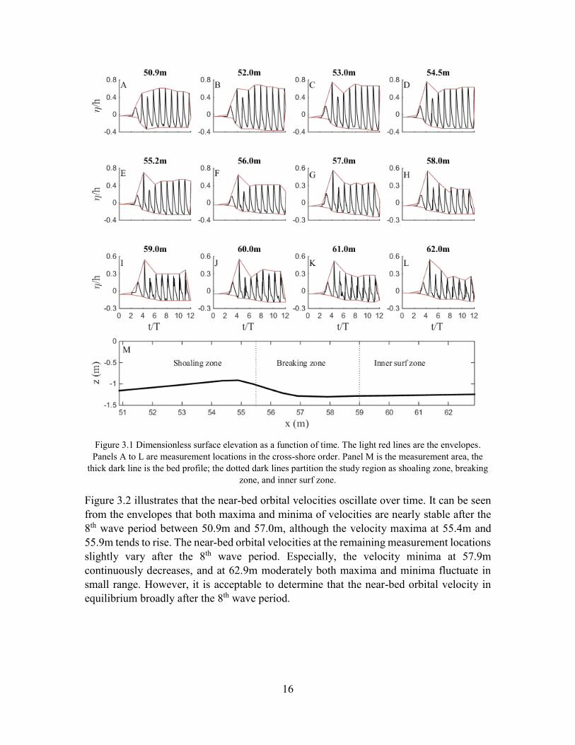
Figure 3.1 Dimensionless surface elevation as a function of time. The light red lines are the envelopes.

Panels A to L are measurement locations in the cross-shore order. Panel M is the measurement area, the

thick dark line is the bed profile; the dotted dark lines partition the study region as shoaling zone, breaking

zone, and inner surf zone.

Figure 3.2 illustrates that the near-bed orbital velocities oscillate over time. It can be seen

from the envelopes that both maxima and minima of velocities are nearly stable after the

8th wave period between 50.9m and 57.0m, although the velocity maxima at 55.4m and

55.9m tends to rise. The near-bed orbital velocities at the remaining measurement locations

slightly vary after the 8th wave period. Especially, the velocity minima at 57.9m

continuously decreases, and at 62.9m moderately both maxima and minima fluctuate in

small range. However, it is acceptable to determine that the near-bed orbital velocity in

equilibrium broadly after the 8th wave period.

17

Figure 3.2 Dimensionless near-bed orbital velocity as a function of time. The light red lines are the

envelopes. Panels A to L are measurement locations in the cross-shore order. Panel M is the measurement

area, the thick dark line is the bed profile; the dotted dark lines partition the study region as shoaling zone,

breaking zone, and inner surf zone.

Figure 3.2 shows the time-dependent depth-averaged turbulence at the measurement

locations. According to the envelopes between 51.0m and 55.0m, it can be seen that the

depth-average turbulence is stable after the 8th wave period. Namely, the depth-average

turbulence in the shoaling zone is in equilibrium after then. When looking at breaking zone

(from 55.5m to 59.0m) and inner surf zone (60.0m and 63.0m), the depth-averaged

turbulence in does not reach the equilibrium until the end of simulation. It likely reaches

equilibrium after the 12th wave period. One thing can be confirmed that the depth-averaged

turbulence in study region takes longer to reach equilibrium than surface elevation and

near-bed orbital velocity. To determine the equilibrium of depth-averaged turbulence, this

research considers more weights on shoaling and breaking zones, because the processes in

inner surf zone is more dynamic and difficult to be reach perfect equilibrium like the other

zones. Therefore, the equilibrium time of depth-averaged turbulence (and the water system)

is determined at the 8th wave period for model validation. Consequently, the time-averaged

18

turbulence in breaking zone and inner surface zone is less accurate, and the quantitative

validation is influenced. However, the qualitative validation is less affected, because it is

done for testing that the at which ADV position the simulated turbulence is the most

reliable.

Figure 3.3 Dimensionless depth-averaged turbulence as a function of time. The light red lines are the

envelopes. Panels A to L are measurement locations in the cross-shore order. Panel M is the measurement

area, the thick dark line is the bed profile; the dotted dark lines partition the study region as shoaling zone,


3.2 Surface elevation

Figure 3.4 compares the phase-averaged surface elevation between wave2Foam and

SINBAD data. Here the normalised root mean square error (NRMSE) is introduced to

facilitate the comparisons between simulated data with different sacels. NRMSE is

calculated as:

19

2

max min

1 1( )i iNRMSE x y

y y N

(3.1)

where N is the amount of time step within one period; x represents dimensional simulated

data; y represents the dimensional experimental data.

Figure 3.4 Comparing dimensionless phase-averaged surface elevation of waves2Fom with SINBAD data.

Panels A to L indicate the locations of PPTs. The normalised root mean square error is represented by

NRMSE. Panel M is the measurement area, the thick dark line is the bed profile; the dotted dark lines

partition the study region as shoaling zone, breaking zone, and inner surf zone.

It can be seen that the simulated phase-averaged elevations broadly match the experimental

data. Moreover, the wave shape transformation is satisfactorily captured by waves2Foam.

The most observable mismatches with average NRMSE of 0.21 are from 54.5m to 56.0m,

where the elevation crests are overestimated. This could be partly caused by surface

tracking process. The phase-averaged simulated surface elevations at the rest locations are

satisfactorily simulated with average NRMSE of approximately 0.15.

20

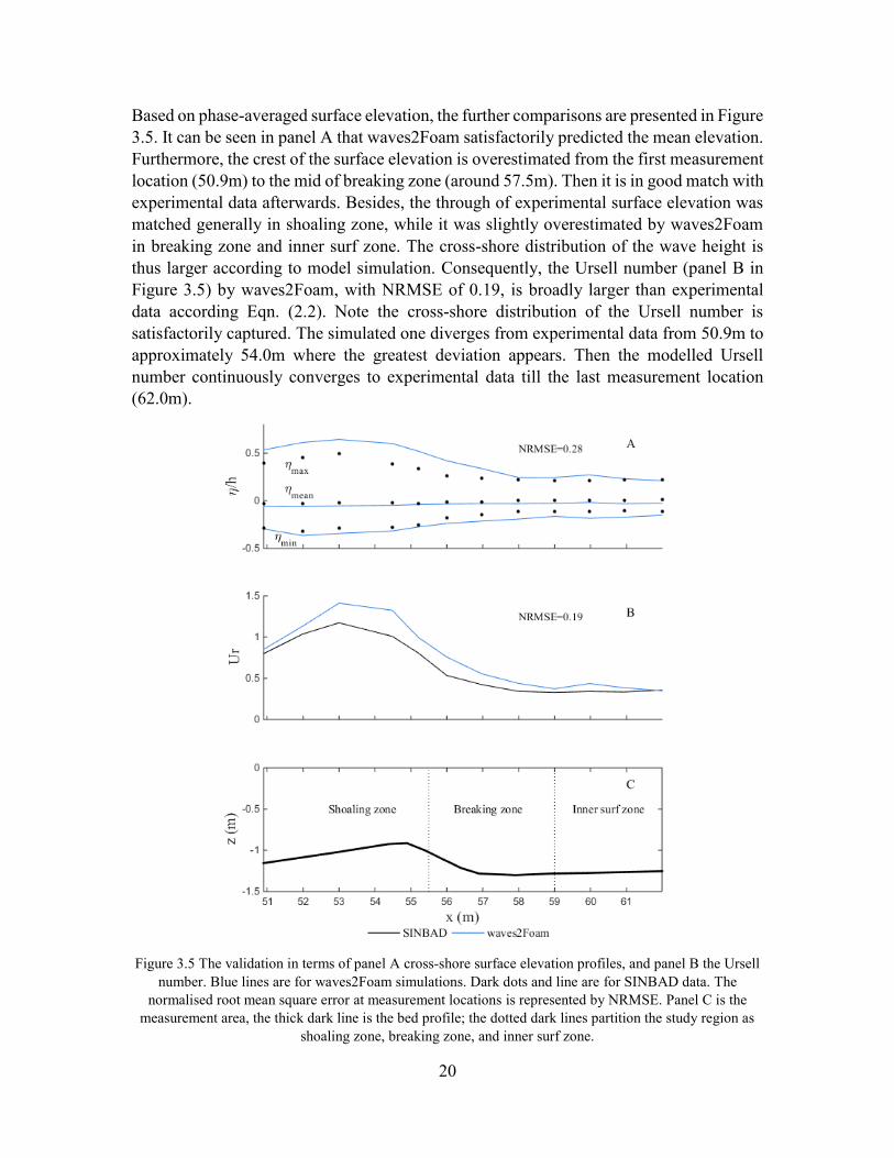
Based on phase-averaged surface elevation, the further comparisons are presented in Figure

3.5. It can be seen in panel A that waves2Foam satisfactorily predicted the mean elevation.

Furthermore, the crest of the surface elevation is overestimated from the first measurement

location (50.9m) to the mid of breaking zone (around 57.5m). Then it is in good match with

experimental data afterwards. Besides, the through of experimental surface elevation was

matched generally in shoaling zone, while it was slightly overestimated by waves2Foam

in breaking zone and inner surf zone. The cross-shore distribution of the wave height is

thus larger according to model simulation. Consequently, the Ursell number (panel B in

Figure 3.5) by waves2Foam, with NRMSE of 0.19, is broadly larger than experimental

data according Eqn. (2.2). Note the cross-shore distribution of the Ursell number is

satisfactorily captured. The simulated one diverges from experimental data from 50.9m to

approximately 54.0m where the greatest deviation appears. Then the modelled Ursell

number continuously converges to experimental data till the last measurement location

(62.0m).

Figure 3.5 The validation in terms of panel A cross-shore surface elevation profiles, and panel B the Ursell

number. Blue lines are for waves2Foam simulations. Dark dots and line are for SINBAD data. The

normalised root mean square error at measurement locations is represented by NRMSE. Panel C is the

measurement area, the thick dark line is the bed profile; the dotted dark lines partition the study region as

shoaling zone, breaking zone, and inner surf zone.

21

3.3 Near-bed orbital velocity

Figure 3.6 compares the dimensionless near-bed orbital velocity among experimental data,

model simulation, and Ruessink parameterisation. NRMSE (Eqn. 3.1) is also applied.

Figure 3.6 Comparing dimensionless phase-averaged near-bed orbital velocity among waves2Fom,

SINBAD data, and Ruessink parameterisation. Panels A to L indicate the locations of lower ADVs. The

normalised root mean square error of waves2Foam and Ruessink parameterisation are represented by

NRMSE1 and NRMSE2. Panel M is the measurement area, the thick dark line is the bed profile; the dotted

dark lines partition the study region as shoaling zone, breaking zone, and inner surf zone.

According to the root mean square error of model simulation (NRMSE1), the most

mismatches of model simulation occur between 50.9m and 54.9m with average RMSE1 of

0.17. Furthermore, after breaking point (55.5m), the simulated velocity shapes are

acceptable with gradually decreasing RMSE1 which is from 0.14 at 55.9m to 0.053 at

22

62.9m which is the best prediction. Then, the root mean square error of Ruessink

parameterisation (NRMSE2) indicates the greatest deviations of velocity shapes at 52.9m

and 54.4m with NRMSE2 of 0.29 and 0.24 respectively. The prediction error of Ruessink

parameterisation fluctuates after (including) 55.4m moderately with mean RMSE2 of

approximately 0.16. Similarly to waves2Foam, the best prediction of Ruessink

parameterisation appear at 62.9m with its minimum RMSE2 of 0.12. Comparing NRMSE1

with NRMSE2, Ruessink parameterisation shows slightly better prediction capacity than

waves2Foam at 50.9m where NRMSE1=0.17, NRMSE2=0.15, and 55.9m where

RMSE1=0.18, RMSE2=0.15. However, for other locations, there is no doubt that

waves2Foam overweighs Ruessink parameterisation regarding NRMSE, which basically

means that the prediction of waves2Foam matches more the pointwise experimental data.

Additionally, comparing NRMSE of modelled surface elevation (Figure 3.4) to NRMSE

of modelled near-bed orbital velocity (Figure 3.6), the later matches better the observations

at corresponding measurement locations.

Panel A in Figure 3.7 illustrates the comparisons of cross-shore velocity profiles. Both

models perform satisfactorily in terms of the prediction of velocity maximum, minimum,

and mean. They predict the cross-shore trends of the velocity profiles with few mismatches,

e.g. the overestimation of maximum in shoaling zone. The profile of experimental mean

velocity is nicely matched, and profiles of both models are overlapped. Note that although

waves2Foam and Ruessink parameterisation compute similarly in terms of the velocity

profiles (NRMSE1=0.16, NRMSE2=0.18), waves2Foam is still more reliable to predict

regular waves. As can be seen from the velocity shapes in Figure 3.6, waves2Foam captures

the cross-shore shape transformation, while Ruessink parameterisation computes

inaccurate peak and trough time points especially in the region after the breaking point. As

results, firstly, in panel B of Figure 3.7, although Ruessink parameterisation shows similar

NRMSE (0.33) with waves2Foam (0.35), it varies in a relatively small range between 0.4

and 0.6, and completely cannot follow the cross-shore trend of skewness under regular

waves. Comparing with Ruessink parameterisation, waves2Foam predicts better in

shoaling and breaking zones, while gives similarly poor results in inner surf zone. Despite

waves2Foam simulates smaller and shifted peak value of skewness in breaking zone, it

qualitatively captures the fluctuating cross-shore trend of skewness. Secondly, it can be

seen in panel C of Figure 3.7 that experimental asymmetry firstly goes down to the lowest

points, then reaches the peak point in breaking zone at similar location with skewness

(57.0m). Afterwards, it has the same trend as skewness. For waves2Foam, the prediction

capacity regarding asymmetry (NRMSE=0.38) is similar with skewness (NRMSE=0.35).

And, waves2Foam acceptably captures the varying cross-shore trend of asymmetry. It can

be noticed that waves2Foam prediction is corresponding shifting probably due to the

slightly shifted peak skewness (panel B). In addition, Ruessink parameterisation results in

relatively large NRMSE of 1.1, because it heavily underestimates the asymmetry of regular

waves in the study region, also it cannot predict the fluctuating cross-shore trend.

23

Figure 3.7 The validation in terms of the near-bed orbital velocity panel A cross-shore profiles, panel B

skewness, and panel C asymmetry. The normalised root mean square error at measurement locations of

waves2Foam and Ruessink parameterisation are represented by NRMSE1 and NRMSE2. Panel C is the

measurement area, the thick dark line is the bed profile; the dotted dark lines partition the study region as

shoaling zone, breaking zone, and inner surf zone.

24

3.4 Turbulence

The time-averaged turbulence vertical profile is evaluated in this section. The mean profiles

of turbulence at all measurements points are larger than the profiles provided by ADVs.

Also, the ADV observation is not always inside the simulated profile envelopes at some

measurement locations. The overestimation of time-averaged turbulence profiles is

common phenomenon for this kind of turbulence model (see Brown et al. 2016).

Figure 3.8 Comparing dimensionless time-averaged turbulence along water column between waves2Fom

and SINBAD data. Panels A to L indicate the average cross-shore location of ADVs. Panel M is the

comparison of time-averaged near-bed turbulence between model simulation and the measurements from

lower ADVs. Panel N is the measurement area, the thick dark line is the bed profile; the dotted dark lines


25

Regarding the experimental measurements, the time-averaged turbulence increases as

ADV is closer to the water surface. Moreover, the time-averaged turbulence profile rises

from 51.0m to 57.0m then drops gradually. Model waves2Foam captures the trend of rising

in x- and z-direction respectively in qualitative way. In x-direction perspective, focusing

on the mean vertical profile, the simulated turbulence experiences the same evolution as

experimental turbulence. According to the profiles, the modelled turbulence increases from

51.0m to 58.0m and reaches the peak, while the peak of experimental profile is at 57.0m.

In z-direction perspective, the overestimation is common at mid and upper ADVs, and it

becomes heavier at upper ADV due to the intense water-air interaction. Throughout the

study region, the simulated time-averaged turbulence is the more reliable at lower ADVs

than mid and upper ADVs, because it overall is the closest to the near-bed observation.

Concerning the time-averaged near-bed turbulence in panel M of Figure 3.8, waves2Foam

broadly overestimates the values with NRMSE of 0.42 which is relaticely larger comparing

with the Ursell number in panel B of Figure 3.5 (NRMSE=0.19), skewness in panel B

(NRMSE=0.35) and in panel C asymmetry (NRMSE=0.38) of Figure3.7. Still,

waves2Foam qualitatively simulates the correct cross-shore profile of the time-averaged

near-bed turbulence. Additionally, it is observable in panel M that a same landwards

shifting for modelled data. This shifting is coincident with other cross-shore trends like

skewness (panel B in Figure 3.7), asymmetry (panel C in Figure 3.7), and vertical

turbulence profiles (panel A to L in Figure 3.8). And the phenomenon of shifting can be

seen as a result of that waves2Foam predicts slightly landwards wave breaking (not shown

here).

3.4 Conclusion

The depth-averaged turbulence is applied to determine the hydrodynamics equilibrium of

waves2Foam simulation, because it takes longer time to reach equilibrium than surface

elevation and near-bed orbital velocity. And the system equilibrium of SINBAD simulation

is determined at the 8th wave period.

For the surface elevation, waves2Foam can simulate the shapes and the transformation with

acceptable NRMSE. Due to the limitation of surface tracking technique, overestimation of

crest profile occurs from shoaling zone to the mid of breaking zone. Moreover, the

overestimation of trough profile occurs in breaking and inner surf zone. Consequently, the

simulated Ursell number is slightly larger than experimental data, but in correct cross-shore

trend. The surface variables are satisfactorily simulated in general.

Under the condition of regular waves, Ruessink parameterisation has similar prediction

capacity with waves2Foam in terms of near-bed orbital velocity maximum, minimum, and

mean. However, according to NRMSE, Ruessink parameterisation matches poorer the

observed velocity shapes than waves2Foam simulation. Moreover, it fails to predict correct

peak and trough time points hence shape transformation, while waves2Foam does much

better. Therefore, waves2Foam overweighs Ruessink parameterisation regarding the

prediction of skewness (in shoaling and breaking zones) and asymmetry for regular waves.

26

As the drawbacks of the applied turbulence model, waves2Foam constantly overestimates

the vertical time-averaged turbulence profiles. Comparing among the time-averaged

turbulence at different positions of ADVs, the near-bed data is more reliable with the least

overestimation. Qualitatively, waves2Foam correctly simulates the development of time-

averaged turbulence profiles both vertically and horizontally. Also, it captures cross-shore

development of the time-averaged near-bed turbulence. The time-averaged turbulence is

less satisfactorily validated. Nonetheless, the more important thing is that the qualitatively

correct cross-shore trend is captured (also for other validated variables). This is good

enough, as this research focuses more on cross-shore trend. Therefore, waves2Foam can

be applied in this research to generate wave data.

27

Chapter 4

Dependencies analysis

Alike to model validation, this chapter starts with the determination of hydrodynamics

equilibrium which facilitate select more periodic wave data for research (Section 4.1). Then,

the dependencies of near-bed skewness and asymmetry on chosen physical parameters are

presented in the order: wave height (Section 4.2); wave length (Section 4.3); the Ursell

number (Section 4.4); surf similarity (Section 4.5); energy dissipation (Section 4.6) which

includes wave energy dissipation, roller dissipation, and dissipation by bed friction; and

near-bed turbulence (Section 4.7). Moreover, depending on different situations, fittings of

dependencies are shown to indicate the simplest linear/non-linear relations between near-

bed skewness and asymmetry and physical parameters.

4.1 Hydrodynamics equilibrium

It is clarified in Section 3.1 of Chapter 3 that, depth-averaged turbulence is introduced to

determine the hydrodynamics equilibrium of model simulation, because it takes longer

time to reaches equilibrium than surface elevation and near-bed orbital velocity. For linear

beds simulations, waves2Foam was stable and simulated runtime of 120s for each case, i.e.

30 waves in total.

Taking case H05T4-SL15 as an example, Figure 4.1 shows the time-dependent depth-

averaged turbulence from the 10th wave period to the 30th. It can be seen in shoaling zone

that, from 40.0m to 46.0m the depth-averaged turbulence reaches the equilibrium at the

15th wave period, while at the 20th wave period at 49.0m and 52.0m. In the breaking zone

(55.0m) and inner surf zone (58.0m and 60.0m), the minimum of depth-averaged

turbulence remains after the 15th wave period, while the maximum is affected by breaking

processes somehow and still fluctuates. However, the maximum at 55.0m varies in

relatively small range and can be seen as equilibrium. Moreover, in the inner surf zone, the

local peaks of upper envelopes are more or less periodic, and are accepted as equilibrium

in this research. For instance, at the most dynamic location 58.0m, the local peaks are

approximately at the 18th, 24th and 28th wave period. Thus, adding the consideration the

equilibrium in shoaling and breaking zones, the equilibrium of depth-averaged turbulence

hence the water system is chosen at the 20th wave period. Namely, 10 waves are selected

for dependencies analysis. Furthermore, the 20th wave period is also considered as when

the equilibrium is reached for other cases. The corresponding figures about time-dependent

depth-averaged turbulence are given in Appendix A.

28

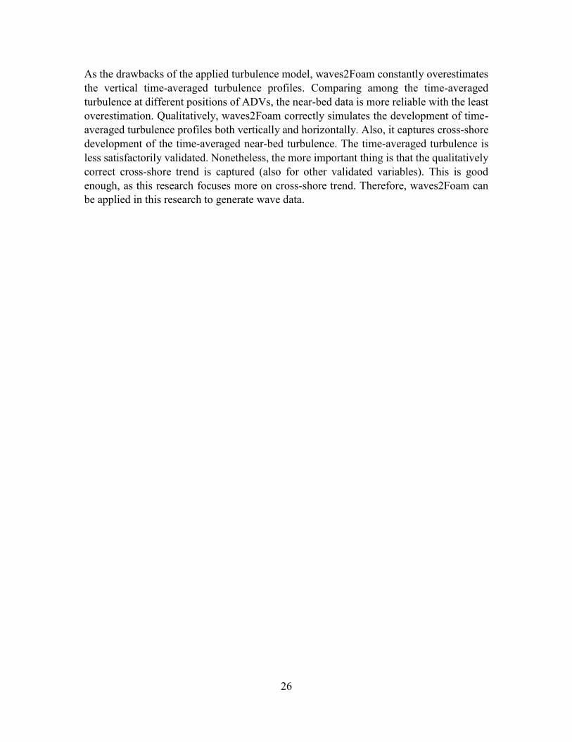
Figure 4.1 Dimensionless depth-averaged turbulence as a function of time of case H05T4-SL15. The light

red lines are the envelopes. Panels A to L are measurement locations in the cross-shore order. Panel M is

the measurement area, the thick dark line is the bed profile; the dotted dark lines partition the study region

as shoaling zone, breaking zone, and inner surf zone.

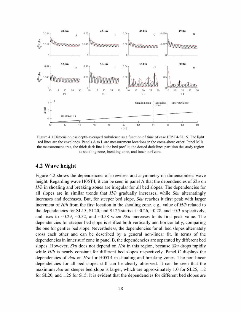
4.2 Wave height

Figure 4.2 shows the dependencies of skewness and asymmetry on dimensionless wave

height. Regarding wave H05T4, it can be seen in panel A that the dependencies of Sku on

H/h in shoaling and breaking zones are irregular for all bed slopes. The dependencies for

all slopes are in similar trends that H/h gradually increases, while Sku alternatingly

increases and decreases. But, for steeper bed slope, Sku reaches it first peak with larger

increment of H/h from the first location in the shoaling zone. e.g., value of H/h related to

the dependencies for SL15, SL20, and SL25 starts at ~0.26, ~0.28, and ~0.3 respectively,

and rises to ~0.29, ~0.52, and ~0.58 when Sku increases to its first peak value. The

dependencies for steeper bed slope is shifted both vertically and horizontally, comparing

the one for gentler bed slope. Nevertheless, the dependencies for all bed slopes alternately

cross each other and can be described by a general non-linear fit. In terms of the

dependencies in inner surf zone in panel B, the dependencies are separated by different bed

slopes. However, Sku does not depend on H/h in this region, because Sku drops rapidly

while H/h is nearly constant for different bed slopes respectively. Panel C displays the

dependencies of Asu on H/h for H05T4 in shoaling and breaking zones. The non-linear

dependencies for all bed slopes still can be clearly observed. It can be seen that the

maximum Asu on steeper bed slope is larger, which are approximately 1.0 for SL25, 1.2

for SL20, and 1.25 for S15. It is evident that the dependencies for different bed slopes are

29

overlapping to large extent. They consequently cluster with linear trend. In panel D, as the

dependencies of Asu on H/h tend to collapse, there is no interesting dependencies can be

seen.

About H08T4, the similar dependencies with slope effect can be observed in shoaling and

breaking zones. In panel E, Sku depends on H/h for all bed slopes are irregular, with the

first at (0.4, 0.4) for SL15, (0.6, 0.62) for SL20, and (0.7, 0.8) for SL25 approximately..

The dependencies for all bed slopes are slightly away from each other, but they still

alternately cross to each other. As a result, non-linear fit can acceptably represent the

general relation of them, however with smaller R2 (0.65) than H05T4 one which is 0.71. In

panel G, the dependencies of Asu on H/h for all bed slopes are slightly scattered than

H05T4 in panel C. Nevertheless, they still cluster with clear linear trend. In addition, there

are no significant dependencies can be found for Sku and Asu in the inner surf zone

respectively.

Figure 4.2 Near-bed orbital velocity skewness (Sku) and asymmetry (Asu) as functions of dimensionless

wave height (H/h) of cases H05T4 and H08T4. Panel A, C, E, and G are the dependencies in shoaling and

breaking zones of corresponding cases. Panel B, D, F, and H are the dependencies in inner surf zone of

corresponding cases. The dark curves/lines are the fittings, with coefficient of determination R2.

4.3 Wavelength

Figure 4.3 shows the dependencies of skewness and asymmetry on dimensionless

wavelength. Focusing on H05T4 firstly, the dependencies for all bed slopes in shoaling and

breaking zones are alike to Sku against H/h in panel A of Figure 4.2, which shows Sku

develops in fluctuating trend with increasing depended L/h. Additionally, the first peak

30

value of Sku is related to larger L/h for gentler bed slope, e.g., roughly, (12, 0.36) for SL15,

(15, 0.6) for SL20, and (16, 0.8) for SL25.

However, Sku against L/h seems like the horizontally compressed Sku against H/h. It can

be therefore fitted by linear function. While in the inner surf zone, panel B displays the

three clearly linear dependencies for different bed slopes respectively. Moreover, Sku

depends on L/h in panel B in an opposite trend against it in panel A. i.e., L/h is positively

correlated to Sku in shoaling and breaking zone, while negative correlation is found in inner

surf zone. In panel C, it can be observed that the pointwise dependencies for all bed slopes

are tightly closed to each other, and cluster to a nearly linear line. And in panel D, Asu in

inner surf zone does not depend on L/h, as it tend to remain with changing L/h.

It can be seen from panel E respectively that, the dependencies of Sku on L/h for the same

bed slope are alike to H05T4 in panel A. The pointwise dependencies for H08T4 for all

bed slopes are more scattered, which still can be acceptably described by a linear function.

This can be also observed when comparing Asu against L/h between H08T4 (panel G) and

H05T4 (panel C). In the inner surf zone, showing the opposite trend against shoaling and

breaking zones, Sku against L/h for H08T4 (panel F) becomes linear and separated by

different bed slopes. Still, there are no interesting relations between Asu and L/h in this

region (panel H).


wave length (L/h) of cases H05T4 and H08T4. Panel A, C, E, and G are the dependencies in shoaling and

breaking zones of corresponding cases. Panel B, D, F, and H are the dependencies in inner surf zone of

corresponding cases. The dark lines are the fittings, with coefficient of determination R2.

31

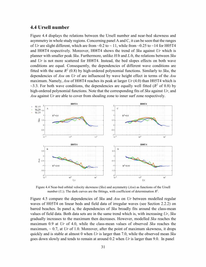
4.4 Ursell number

Figure 4.4 displays the relations between the Ursell number and near-bed skewness and

asymmetry in whole study regions. Concerning panel A and C, it can be seen that the ranges

of Ur are slight different, which are from ~0.2 to ~ 11, while from ~0.25 to ~14 for H05T4

and H08T4 respectively. Moreover, H08T4 shows the trend of Sku against Ur which is

planner with smaller peak Sku. Furthermore, unlike H/h and L/h, the relations between Sku

and Ur is not more scattered for H08T4. Instead, the bed slopes effects on both wave

conditions are equal. Consequently, the dependencies of different wave conditions are

fitted with the same R2 (0.8) by high-ordered polynomial functions. Similarly to Sku, the

dependencies of Asu on Ur of are influenced by wave height effect in terms of the Asu

maximum. Namely, Asu of H08T4 reaches its peak at larger Ur (4.0) than H05T4 which is

~3.3. For both wave conditions, the dependencies are equally well fitted (R2 of 0.8) by

high-ordered polynomial functions. Note that the corresponding fits of Sku against Ur, and

Asu against Ur are able to cover from shoaling zone to inner surf zone respectively.

Figure 4.4 Near-bed orbital velocity skewness (Sku) and asymmetry (Asu) as functions of the Ursell

number (Ur). The dark curves are the fittings, with coefficient of determination R2.

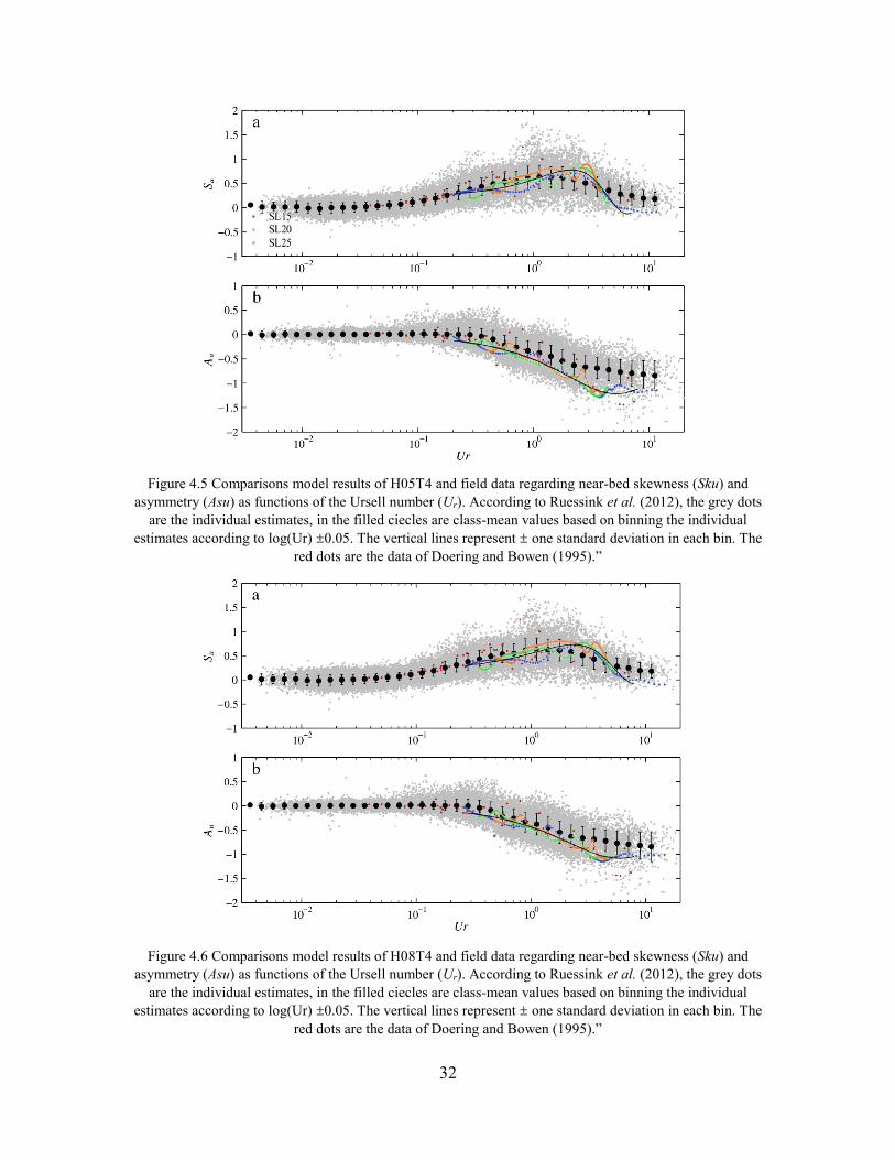
Figure 4.5 compare the dependencies of Sku and Asu on Ur between modelled regular

waves of H05T4 on linear beds and field data of irregular waves (see Section 2.2.2) on

barred beaches. In panel a, the dependencies of Sku broadly fits around the class-mean

values of field data. Both data sets are in the same trend which is, with increasing Ur, Sku

gradually increases to the maximum then decreases. However, modelled Sku reaches the

maximum 0.9 at Ur of 4.0, while the class-mean values of observed Sku reaches the

maximum, ~ 0.7, at Ur of 1.0. Moreover, after the point of maximum skewness, it drops

quickly and is stable at almost 0 when Ur is larger than 7.0, while the observed mean Sku

goes down slowly and tends to remain at around 0.2 when Ur is larger than 9.0. In panel

32

Figure 4.5 Comparisons model results of H05T4 and field data regarding near-bed skewness (Sku) and

asymmetry (Asu) as functions of the Ursell number (Ur). According to Ruessink et al. (2012), the grey dots

are the individual estimates, in the filled ciecles are class-mean values based on binning the individual

estimates according to log(Ur) ±0.05. The vertical lines represent ± one standard deviation in each bin. The

red dots are the data of Doering and Bowen (1995).”

Figure 4.6 Comparisons model results of H08T4 and field data regarding near-bed skewness (Sku) and

asymmetry (Asu) as functions of the Ursell number (Ur). According to Ruessink et al. (2012), the grey dots

are the individual estimates, in the filled ciecles are class-mean values based on binning the individual

estimates according to log(Ur) ±0.05. The vertical lines represent ± one standard deviation in each bin. The

red dots are the data of Doering and Bowen (1995).”

33

b, the dependencies of Asu does not well fit the class-mean values of field data. It can be

seen that the modelled Asu is broadly larger than the class-mean values between Ur of 0.2

and 10.0. Besides, the modelled Asu experiences the same trend as Sku, i.e., with

continuously rising Ur, Asu increases to the maximum (-1.3) then decrease, which is

followed by keeping at ~ -1.2 with Ur of 7.0. Interestingly, for the dependencies of Asu of

irregular waves on barred beaches, neither all the individual measurement nor the class-

mean values show this trend. Instead, observed class-mean Asu rises from 0 at Ur of 0.2 to

0.7 at Ur of 8.0 approximately, then remains at the same level.

Since the differences of dependencies of Sku and Asu between H05T4 and H08T4 are

subtle (Figure 4.2), the comparisons regarding H08T4 and field data in Figure 4.6 present

nearly the same results as H05T4 in Figure 4.5. According to the comparisons in Figure

4.4 and 4.5, it can be thus said that for the regular waves on linear beds, Sku and Asu is

related to Ur differently with irregular waves on barred beds to some extent.

4.5 Surf similarity parameter

The dependencies of near-bed skewness and asymmetry on surf similarity parameter are

presented in Figure 4.7. The bed slope effect on the dependencies in Figure 4.7 is

significant throughout the study area. There is no overlapping among the pointwise

dependencies for different slopes in each panel of Figure 4.7. Therefore, in each panel, the

dependencies for different bed slopes can only be fitted respectively, and no general fit can

be obtained. For instance, about H05T4, panel A displays that the separated dependencies

for different bed slopes are fitted by different linear lines respectively. These linear trend

lines are resolved best fits, but they cannot adequately represent the irregular pointwise

dependencies. In inner surf zone (panel B), the dependencies for different bed slopes

become linear and parallel to each other with the coincident trend with shoaling and

breaking zones. In panel C, the dependencies of Asu on ξ for different bed slopes are

acceptably represented by the linear fits respectively. As can be seen from the fits in panel

A and C, the fit for SL25 is the steepest, which means that both Sku and Asu are more

sensitive to the change of ξ on gentler bed slope. Under the same case, the dependencies of

Sku and Asu for H08T4 are correspondingly alike to H05T4. The wave height effect can

be viewed more clearly in the shoaling and breaking zones. For the same bed slope, say

SL15, the Sku against ξ between H05T4 (panel A) shows a milder trend than H08T4 (panel

E), which indicates that the dependencies is more sensitive to waves with higher H.

Despite the dependencies in Figure 4.7 are clear and can be simply fitted, they are not

favourable for parameterisation. Because, firstly the relations between Sku and ξ are

irregular and cannot be described by linear fits properly; secondly, strong bed slope effect

makes situation complicated, i.e., the parameterisation (if there were) has the limitation

about the validity regime. However, it is still a good parameter for one who wants to

incorporate the bed slope effect in parameterisation.

34

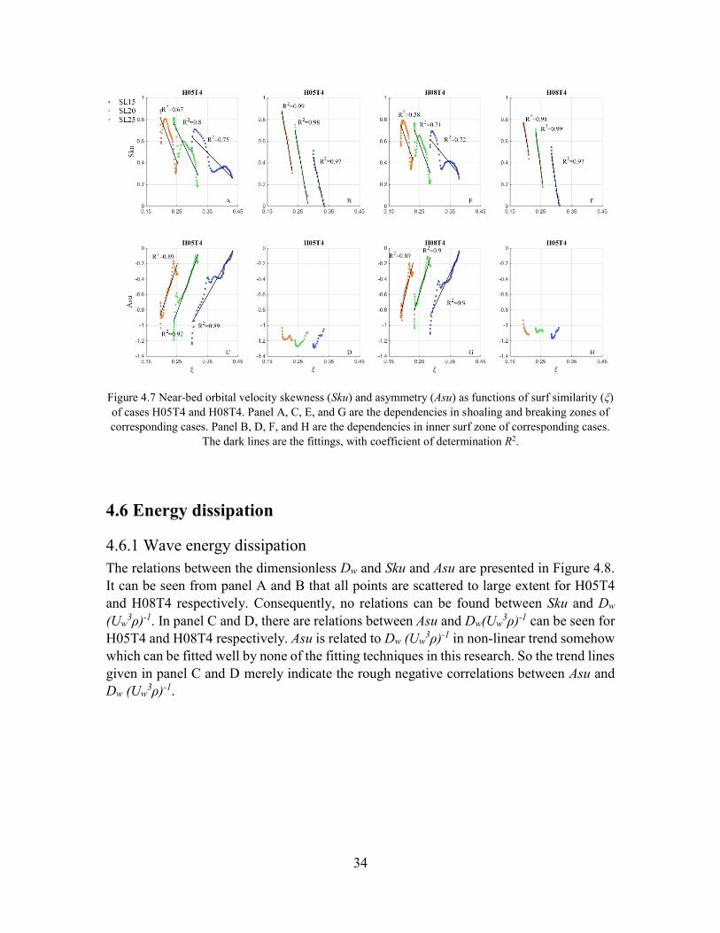
Figure 4.7 Near-bed orbital velocity skewness (Sku) and asymmetry (Asu) as functions of surf similarity (ξ)

of cases H05T4 and H08T4. Panel A, C, E, and G are the dependencies in shoaling and breaking zones of

corresponding cases. Panel B, D, F, and H are the dependencies in inner surf zone of corresponding cases.

The dark lines are the fittings, with coefficient of determination R2.

4.6 Energy dissipation

4.6.1 Wave energy dissipation

The relations between the dimensionless Dw and Sku and Asu are presented in Figure 4.8.

It can be seen from panel A and B that all points are scattered to large extent for H05T4

and H08T4 respectively. Consequently, no relations can be found between Sku and Dw

(Uw3ρ)-1. In panel C and D, there are relations between Asu and Dw(Uw

3ρ)-1 can be seen for

H05T4 and H08T4 respectively. Asu is related to Dw (Uw3ρ)-1 in non-linear trend somehow

which can be fitted well by none of the fitting techniques in this research. So the trend lines

given in panel C and D merely indicate the rough negative correlations between Asu and

Dw (Uw3ρ)-1.

35


wave energy dissipation (Dw (Uw3ρ)-1) of cases H05T4 and H08T4. The dark curves/lines are the fittings,

with coefficient of determination R2.

4.6.2 Roller dissipation

The dependencies of skewness and asymmetry on dimensionless roller dissipation are

presented in Figure 4.9. Since Dr (Uw3ρ)-1 is a turbulence related term and independent

from basic wave parameters, there are some new non-linear dependencies of Sku and Asu

on Dr (Uw3ρ)-1 shown in shoaling and breaking zones. For H05T4, it can be observed from

panel A and C that no slope effect appears. Furthermore, the fits satisfactorily describe that

Sku and Asu exponentially decay with increasing Dr (Uw3ρ)-1 in panel A and C respectively.

While in inner surf zone, the relations between Sku and Dr (Uw3ρ)-1 becomes relatively

linear for all different bed slopes. While Asu does not depend on Dr (Uw3ρ)-1 in this region,

because Dr (Uw3ρ)-1 here varies in very small range (between 0 and ~0.3×10-4) and Asu is

almost constant. Since the relations between Asu and Dr (Uw3ρ)-1 in inner surf zone contains

very small weight among the pointwise dependencies in whole study area, they could be

36

neglected for fitting. Therefore, the fit in panel C can be considered to be able to represent

dependencies of Asu on Dr (Uw3ρ)-1 from shoaling zone to inner surf zone.

Comparing with H05T4, the pointwise dependencies of Sku and Asu for H08T4 in shoaling

and breaking zones are more scattered, as result they are fitted exponentially with smaller

R2. The fit in panel G could be used to describe the Asu against Dr (Uw3ρ)-1 in whole study

area, for the same reason as H05T4. Moreover, in shoaling and breaking zones, Sku (Asu)

for H05T4 exponentially decay with increase Dr (Uw3ρ)-1 than H08T4. Besides, in inner

surf zone, the trends of Sku against Dr (Uw3ρ)-1 for H05T4 are broadly steeper than H08T4.

Hence, it can be said that Sku (Asu) is more sensitive to the change of Dr (Uw3ρ)-1 for the

waves with smaller H.


roller dissipation (Dr (Uw3ρ)-1) of cases H05T4 and H08T4. Panel A, C, E, and G are the dependencies in

shoaling and breaking zones of corresponding cases. Panel B, D, F, and H are the dependencies in inner surf

zone of corresponding cases. The dark curves/lines are the fittings, with coefficient of determination R2.

4.6.3 Dissipation due to bed friction

Figure 4.2 illustrates the dependencies of near-bed skewness and asymmetry on dissipation

due to bed friction. It can be seen in shoaling and breaking zones, the dependencies of Sku

and Asu on Df (Uw3ρ)-1 are alike to the dependencies on H/h (Figure 4.2) and on L/h (Figure

4.3) to some extent. However, the dependencies on Dr (Uw3ρ)-1 are more complex and

irregular so that their trends are less clear. For example, in panel A, the dependencies for

different bed slopes converge at point (0.8×10-3, 0.3), then they diverge with increasing

Sku and Df(Uw3ρ)-1 in very curvy ways respectively. And the dependencies are more

sensitive on gentler bed slope. The R2 of the fits for different bed slopes seems to be

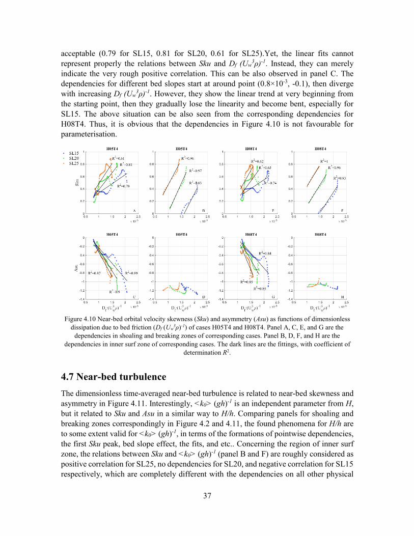
37

acceptable (0.79 for SL15, 0.81 for SL20, 0.61 for SL25).Yet, the linear fits cannot

represent properly the relations between Sku and Df (Uw3ρ)-1. Instead, they can merely

indicate the very rough positive correlation. This can be also observed in panel C. The

dependencies for different bed slopes start at around point (0.8×10-3, -0.1), then diverge

with increasing Df (Uw3ρ)-1. However, they show the linear trend at very beginning from

the starting point, then they gradually lose the linearity and become bent, especially for

SL15. The above situation can be also seen from the corresponding dependencies for

H08T4. Thus, it is obvious that the dependencies in Figure 4.10 is not favourable for

parameterisation.


dissipation due to bed friction (Df (Uw3ρ)-1) of cases H05T4 and H08T4. Panel A, C, E, and G are the

dependencies in shoaling and breaking zones of corresponding cases. Panel B, D, F, and H are the

dependencies in inner surf zone of corresponding cases. The dark lines are the fittings, with coefficient of

determination R2.

4.7 Near-bed turbulence

The dimensionless time-averaged near-bed turbulence is related to near-bed skewness and

asymmetry in Figure 4.11. Interestingly, <k0> (gh)-1 is an independent parameter from H,

but it related to Sku and Asu in a similar way to H/h. Comparing panels for shoaling and

breaking zones correspondingly in Figure 4.2 and 4.11, the found phenomena for H/h are

to some extent valid for <k0> (gh)-1, in terms of the formations of pointwise dependencies,

the first Sku peak, bed slope effect, the fits, and etc.. Concerning the region of inner surf

zone, the relations between Sku and <k0> (gh)-1 (panel B and F) are roughly considered as

positive correlation for SL25, no dependencies for SL20, and negative correlation for SL15

respectively, which are completely different with the dependencies on all other physical

38

parameters which are in coincident trend in this region. Additionally, it can be seen from

panel D and H that the relations between Asu and <k0> (gh)-1 in inner surf zone are not

interesting. So far, it is common that no favourable relations can be found between Asu and

one physical parameter in inner surf zone. Under the condition of regular waves on linear

beds, <k0> (gh)-1 is related to Sku and Asu in similar ways to H/h. The information of <k0>

(gh)-1 probably is embedded in H/h. Therefore, H/h can be a good alternative to <k0> (gh)-

1 for parameterisation.


time-averaged near-bed turbulence (<k0> (gh)-1) of cases H05T4 and H08T4. Panel A, C, E, and G are the

dependencies in shoaling and breaking zones of corresponding cases. Panel B, D, F, and H are the

dependencies in inner surf zone of corresponding cases. The dark curves/lines are the fittings, with

coefficient of determination R2.

4.8 Conclusion

According to the analysis in this Chapter, ξ, Dw(Uw3ρ)-1 and Df (Uw

3ρ)-1 are not suitable for

parameterisation. Because, firstly, mainly the relations between Sku (Asu) and ξ depend

largely on bed slope, which gives complex validity regime for parameterisation; secondly,

there is no relation between Sku and Dw(Uw3ρ)-1 due to highly scattered pointwise

dependencies. Moreover, the relation between Asu and Dw(Uw3ρ)-1 cannot be satisfactorily

fitted. Thirdly, the dependencies of Sku and Asu on Df (Uw3ρ)-1 in shoaling and breaking

zones are too complex and irregular to derive a parameterisation.

The dependencies of Sku and Asu on the rest physical parameters can be observed and fitted

respectively. But note that in inner surf zone, Asu does not depend on all of them, but Ur

and Dr (Uw3ρ)-1. Furthermore, <k0> (gh)-1

is related to Sku and Asu similarly to H/h. This

39

is only valid under the condition of regular waves on linear beds (slope bigger than1/25).

Thus, as a simpler parameter, H/h is a better choice than <k0> (gh)-1 for parameterisation.

Finally, the suggested parameters for further analysis on parameterisation are H/h, L/h, Ur,

and Dr (Uw3ρ)-1. And they will be discussed in the next Chapter.

41

Chapter 5

Discussion

To parameterise near-bed skewness and asymmetry for practical use, there two

considerations. On one hand, chosen physical parameter should be related to near-bed

skewness and asymmetry in the trend, which can be satisfactorily fitted by relatively simple

trend lines. On the other hand, the chosen parameter should be as simple as possible.

Table 5.1 shows R2 of these dependencies in order to exam and compare how well

dependencies of Sku and Asu on selected parameters can be fitted respectively. Firstly, the

general fits can be found to represent the dependencies of Sku on a physical parameter for

all bed slops in shoaling and breaking zones. The R2 is ranked as: Ur, Dr (Uw3ρ)-1, L/h, H/h,

from high to low, which indicates that it is better to introduce Ur or Dr (Uw3ρ)-1 in

parameterisations of Sku, instead of directly using simple parameters H/h or L/h in this

region. Moreover, in inner surf zone, Sku does not depend on H/h. And, it linearly depends

on the Dr (Uw3ρ)-1(Figure 4.9), and L/h (Figure 4.3) with the slope effects, thus there are

three fits for different bed slopes respectively. Furthermore, Ur is related to Sku in a single

non-linear trend without slope effects in whole study region (Figure 4.4).

Secondly, for Asu, the dependencies on Dr (Uw3ρ)-1, and Ur can be described by one

function respectively in the whole study region. The dependencies on H/h and L/h can be

fitted satisfactorily respectively, only in shoaling and breaking zones. However, there is

nothing interesting between Asu and H/h and L/h respectively in the inner surf zone.

Thirdly, the relations between Ur and Sku and Asu are not influenced by wave height effect.

For both H05T4 and H08T4, R2 keeps at 0.8 for Sku and 0.95 for Asu respectively.

For the other physical parameters, in shoaling and breaking zones, the fits for the

dependencies are better for H05T4 than H08T4 in terms of Sku and Asu respectively. As

shown in corresponding figures in Chapter 4, this is because the pointwise dependencies

are more scattered when the input wave height is higher, the fits hence less match them.

Moreover, the dependencies of Sku on physical parameters is more sensitive to wave height

effects than Asu. Namely, the differences R2 regarding dependencies of Sku between

H05T4 and H08T4 are broadly larger. For instance, R2 for Sku against H/h varies from 0.71

for H05T4 to 0.65 for H08T4, while R2 changes from 0.93 for H05T4 to 0.92 for H08T4

for Asu against H/h. In inner surf zone, the wave height does not impact on the

dependencies.

42

Table 5.1 The list of R2 of resolved best fits of the dependencies of Sku and Asu on chosen physical

parameters for all cases. “-” means no interesting dependencies.

Wave

condition

Region

of

Bed

slope H/h L/h Ur Dr (Uw3ρ)-1

Shoaling 1/15

& 1/20 0.71 0.74 0.79

H05T4 breaking 1/25 0.8

1/15 0.99 0.97

Inner-surfing 1/20 - 0.99 0.88

1/25 0.99 0.87

Sku Shoaling 1/15

& 1/20 0.65 0.63 0.72

breaking 1/25 0.8

H08T4 1/15 0.98 0.98

Inner-surfing 1/20 - 1.00 0.91

1/25 0.98 0.87

Shoaling 1/15

& 1/20 0.93 0.90

H05T4 breaking 1/25 0.95 ~0.88

1/15

Inner-surfing 1/20 - - Asu 1/25

Shoaling 1/15

& 1/20 0.92 0.88

H08T4 breaking 1/25 0.95 ~0.82

1/15

Inner-surfing 1/20 - - 1/25

According to the above analysis, Ur, and Dr (Uw3ρ)-1 are better physical parameters related

to Sku and Asu. And they are potential to be applied in the parameterisation of Sku and Asu

under condition of regular waves propagating on linear beds. The Ursell number is

computed from wave height and wave number, so it can be simply applied in

parameterisation according the Ruesskin’s work. However, Dr (Uw3ρ)-1 is a complex

parameter which is impossible to be directly used in parameterisation. Therefore, Figure

5.1 presents the link between Dr(Uw3ρ)-1 and basic wave parameters. It can be seen in Figure

5.1 that, it is evident that H/h and L/h are the functions of Dr(Uw3ρ)-1 respectively, i.e. there

is the possibility to express Dr(Uw3ρ)-1 with H/h and L/h. Therefore, a brand-new idea is

arouse to include the effect of roller dissipation in the parameterisation of near-bed

skewness and asymmetry. This hypothesis is required to be further researched.

43

Figure 5.1 Dimensionless wave height (H/h) and dimensionless wave length (L/h) as functions of

dimensionless roller dissipation (Dr (Uw3ρ)-1) of cases H05T4 and H08T4 respecticely.The dark curves are

the fittings, with coefficient of determination R2.

45

Chapter 6

Conclusion and recommendations

6.1 Conclusion

The research objective of this research is presented in Section 1.2. It is:

To determine wave shoaling and breaking effects on the near-bed orbital velocity skewness

and asymmetry in order to improve the orbital velocity parameterisation by Ruessink et al.

(2012).

Just after the research objective, the research objective, the relative research question and

sub-questions are presented in Section 1.2. The objective is achieved by answering the

research questions as follow:

How well can wave2Foam simulate near-bed orbital velocity under regular waves?

The observed data from the SINBAD mobile bed CIEM wave flume experiment (H=0.85m,

T=4.0s) with barred beach with foreslope of 1/10 is used to validate the numerical model

waves2Foam. The surface elevation, near-bed orbital velocity, and turbulence were

measured at 12 cross-shore locations from shoaling zone to inner surf zone. Velocity and

turbulence were measured at 3 vertical positions at each cross-shore location.

For the surface elevation, waves2Foam can simulate the shapes and the transformation with

acceptable NRMSE. But, it overestimation of crest profile occurs from shoaling zone to

the mid of breaking zone, while the overestimation of trough profile occurs in breaking and

inner surf zone. Consequently, the simulated Ursell number with correct cross-shore trend,

is larger than experimental data quantitatively. The surface variables are satisfactorily

simulated in general.

Under the condition of regular waves, waves2Foam is able to predicts the near-bed orbital

velocity maximum, minimum, and mean broadly. Moreover, the simulated velocity shape

matches acceptably the experiment velocity shapes. It is important that it is able to capture

the velocity shape transformation. As results, the simulated near-bed asymmetry is

satisfactorily validated to experimental data. And, the simulated near-bed skewness is

validated from the shoaling zone to the right boundary of breaking zone, while is not

validated in inner surf zone.

The waves2Foam constantly overestimates the vertical time-averaged turbulence profiles.

Comparing among the time-averaged turbulence at different positions of ADVs, the near-

bed data is more reliable with the least overestimation. Qualitatively, waves2Foam

correctly simulates the development of time-averaged turbulence profiles both vertically

and horizontally. Also, it captures cross-shore development of the time-averaged near-bed

46

turbulence. The time-averaged turbulence is less satisfactorily validated. Nonetheless, the

more important thing is that the qualitatively correct cross-shore trend is captured.

Despite waves2Foam simulates the wave with some deviations regarding the values

according to the above, it can broadly capture the cross-shore distributions in terms of surf

elevation, near-bed skewness and asymmetry, the Ursell number, and etc.. As the cross-

shore trend is more important in this research, therefore waves2Foam can be used.

How do wave shoaling and breaking affect the near-bed orbital velocity?

The physical parameters applied in this research are: wave height, wavelength, surf

similarity parameter, the Ursell number, wave energy dissipation, roller dissipation,

dissipation due to bed friction, and near-bed turbulence. The dependencies of near-bed

skewness and asymmetry on wave energy dissipation and dissipation by bed friction are

evident respectively, thus they are not favourable for parameterisation. Moreover, the

dependencies on surf similarity are strongly influenced by bed slope effect, which results

in the dependencies for all the cases need to be fitted respectively.

For the rest physical parameters – wave height, wave length, the Ursell number, roller

dissipation, and near-bed turbulence – the bed slope effect is weak on them in shoaling and

breaking zones. Thus there are always general trends can be found for these physical

parameters respectively. The dependencies on them show steeper trend for H05T4 than

H08T4, i.e., both near-bed skewness and asymmetry are more sensitive to depended

parameters when wave height is smaller. In inner surf zone, the dependencies of near-

skewness on them (except the Ursell number) affected by the bed slope effect and are

constantly linear. The near-bed asymmetry only depend on the Ursell number and roller

dissipation.

How can the Ruessink parameterisation be improved?

In this research, under the condition of regular waves on linear beds (slope bigger than

1/25), the Ursell number and roller dissipation are selected for parameterisation. It can refer

the idea of Ruessink’ work to parameterise near-bed skewness and asymmetry by Ursell

number, under the condition of regular waves on linear beds with slope bigger than 1/25.

Additionally, as the roller dissipation can be expressed by basic wave parameters, like wave

height and wavelength. It illustrates the possibility of involving a new process in

parameterisation. The potential parameterisation could help Ruessink’ method, but it need

to be deeper studied.

47

6.2 Recommendations

A number of recommendations is presented to facilitate an improved Ruessink

parameterisation.

Firstly, in terms of the parameterisation, the Ursell number is the first option for as it can

be relatively applied in existing Ruessink parameterisation. And, it overweighs other

physical parameters in terms of the extent of being influenced by the wave height effect

and bed slope effect. Furthermore, it is still in great interests to involve a new physical

process in parameterisation in further research. The roller dissipation is possible to be

applied in parameterisation, because it is the function of wave height and wavelength

respectively, under the condition in this research. However, one should be careful when

deriving the parametrisation for near-bed skewness. Because, the dependencies in shoaling

and breaking zones are exponential, while linear in inner surf zone. Besides, the

dependencies of near-bed skewness and asymmetry of the roller dissipation are influenced

by the wave height effect. This could result in a validity regime regarding wave height.

Secondly, the dependencies from six case studies is inadequately to derive a

parameterisation. It is suggested to take into account other input wave heights and linear

bed (slope smaller than 1/25). It is also important to including other conditions, like long

waves, because long waves behave differently with short waves regarding cross-shore

distributions of near-bed skewness and asymmetry (Fernandez-Mora. 2015); also the

barred beach.

Thirdly, in this research, the accuracy of surface elevation (by the method in Appendix B.1)

could be affected to some extent, as well as the relative variables like wave height, the

Ursell number, surf similarity, and etc.. Therefore, an improved tracking techniques of free

surface is in necessity.

49

References

Abreu, T., Silva, P. A., Sancho, F., and Temperville, A. (2010). Analytical approximate wave form

for asymmetric waves. Coastal Engineering, 57(7), 656-667.

Battjes, J. A. (1974), Surf similarity parameter. Coastal Engineering Proceedings International

Conference on Coastal Engineering, no.14, 466-480.

Battjes, J. A., and Janssen, J. P. F. M. (1978). Energy loss and set-up due to breaking of random

waves. Coastal Engineering Proceedings, 1(16).

Brown, S. A., Greaves, D. M., Magar, V., and Conley, D. C. (2016). Evaluation of turbulence

closure models under spilling and plunging breakers in the surf zone. Coastal Engineering, 114,

177-193.

Christensen, E. D., and Deigaard, R. (2001). Large eddy simulation of breaking waves. Coastal

engineering, 42(1), 53-86.

Drake, T. G., and Calantoni, J. (2001). Discrete particle model for sheet flow sediment transport in

the nearshore. Journal of Geophysical Research: Oceans, 106(C9), 19859-19868.

Doering, J. C., and Bowen, A. J. (1995). Parametrization of orbital velocity asymmetries of

shoaling and breaking waves using bispectral analysis. Coastal Engineering, 26(1-2), 15–33.

Elfrink, B., Hanes, D. M., and Ruessink, B. G. (2006). Parameterisation and simulation of near bed

orbital velocities under irregular waves in shallow water. Coastal Engineering, 53(11), 915-

927.

Elgar, S., Gallagher, E. L., and Guza, R. T. (2001). Nearshore sandbar migration. Journal of

Geophysical Research. C. Oceans, 106, 11623-11627.

Elgar, S. (1987). Relationships involving third moments and bispectra of a harmonic process. IEEE

transactions on acoustics, speech, and signal processing, 35(12), 1725-1726.

Fernandez-Mora A., (2015). On cross-shore beach profile morphodynamics. Universitat

Politecnica de Caralunya. PhD Thesis.

Guza, R. T., and Thornton, E. B. (1980). Local and shoaled comparisons of sea surface elevations,

pressures, and velocities. Journal of Geophysical Research: Oceans, 85(C3), 1524-1530.

Isobe, M., and Horikawa, K. (1982). Study on water particle velocities of shoaling and breaking

waves. Coastal Engineering in Japan, 25, 109-123.

Jacobsen, N. G., Fuhrman, D. R., and Fredsøe, J. (2012). A wave generation toolbox for the open‐source CFD library: OpenFoam®. International Journal for Numerical Methods in

Fluids, 70(9), 1073-1088.

50

Kennedy, A. B., Chen, Q., Kirby, J. T., and Dalrymple, R. A. (2000). Boussinesq modeling of wave

transformation, breaking, and runup. I: 1D. Journal of waterway, port, coastal, and ocean

engineering, 126(1), 39-47.

Kim, J., Moin, P., and Moser, R. (1987). Turbulence statistics in fully developed channel flow at

low Reynolds number. Journal of fluid mechanics, 177, 133-166.

Malarkey, J., and Davies, A. G. (2012). Free-stream velocity descriptions under waves with

skewness and asymmetry. Coastal Engineering, 68, 78-95.

Manual, S. P. (1984). Department of the Army, Waterways Experiment Station, Corps of

Engineers. Coastal engineering researcher center, 2.

Ruessink, B. G., Michallet, H., Abreu, T., Sancho, F., Van der Werf, J. J., and Silva, P. A. (2011).

Observations of velocities, sand concentrations, and fluxes under velocity‐asymmetric

oscillatory flows. Journal of Geophysical Research: Oceans, 116(C3).

Ruessink, B. G., Ramaekers, G., and Van Rijn, L. C. (2012). On the parameterisation of the free-

stream non-linear wave orbital motion in nearshore morphodynamic models. Coastal

Engineering, 65, 56-63.

Svendsen, I. A. (1984). Wave heights and set-up in a surf zone. Coastal Engineering, 8(4), 303-

329.

Svendsen, I. A. (1987). Analysis of surf zone turbulence. Journal of Geophysical Research:

Oceans, 92(C5), 5115-5124.

Van der A.D., van der Zanden J., O’Donoghue, T., Hunter D., Cáceres, I., McLelland, J.S., and

Ribberink, J. S. (to be submitted). Hydrodynamics and turbulence under a large-scale plunging

wave over a fixed bar.

Van den Broek. (2015). Water Particle Velocities under Shoaling and Breaking Waves. University

of Twente. Bsc. Thesis.

Van der Zanden, J., Van der A, D. A., Hurther, D., Cáceres, I., O'Donoghue, T., and Ribberink, J.

S. (2016). Near‐bed hydrodynamics and turbulence below a large‐scale plunging breaking wave

over a mobile barred bed profile.Journal of Geophysical Research: Oceans.

51

List of symbols

The following are main symbols presented in this thesis. Other symbols are also used and

defined in the text.

0u : Horizontal near-bed orbital velocity, m/s

wU : Amplitude of near-bed orbital velocity, m/s

Sku : Skewness of horizontal near-bed orbital velocity, dimensionless

Asu : Asymmetry of horizontal near-bed orbital velocity, dimensionless

rU : Ursell number, dimensionless

T : Wave period, s

: Angular frequency of wave, dimensionless

H : Wave height, m

L : Wavelength, m

h : Water depth, m

: Surface elevation, m

: Density of sea water, kg/m3

g : Gravitational acceleration, m/s2

: Surf similarity, dimensionless

0

Hk : Depth-averaged turbulence from bed to the lower surface elevation profile, m2/s2

0k : Near-bed turbulence, m2/s2

: Eddy viscosity, m2/s

wE : Total wave energy, J/m2

wD : Total wave energy dissipation, J/m2/s

rD : Roller dissipation, J/m2/s

fD : Dissipation due to friction, J/m2/s

53

List of Figures

Figure 1.1 The comparisons of the near-bed orbital velocity between sinusoidal shape and,

panel A pure skewed shape, and panel B pure asymmetric shape. The near-bed orbital

velocity is calculated by the expression in Abreu et al. (2010).

Figure 2.1“Bed profile and measuring locations. (a) General overview of wave flume,

including initial horizontal test section (dotted line), reference bed profile (solid bold black

line), fixed beach (solid gray line) and locations of resistive wave gauges (black vertical

lines, not at full scale); (b) Close-up of test section, including reference bed profile and

instrument positions: mobile-frame pressure transducer (‘PT mob’.; white squares); wall-

deployed PTs (black squares); mobile-frame ADVs (stars); and ACVP sampling profiles

(gray rectangles).” (Source: Van der Zanden et al. 2016)

Figure 2.2 The designed linear sloping bed profiles (dark thick lines) with slope, panel A

1/15, panel B 1/20, and Panel C 1/25. The blue dashed lines are the still water level.

Figure 3.1 Dimensionless surface elevation as a function of time. The light red lines are

the envelopes. Panels A to L are measurement locations in the cross-shore order. Panel M

is the measurement area, the thick dark line is the bed profile; the dotted dark lines partition

the study region as shoaling zone, breaking zone, and inner surf zone.

Figure 3.2 Dimensionless near-bed orbital velocity as a function of time. The light red lines

are the envelopes. Panels A to L are measurement locations in the cross-shore order. Panel

M is the measurement area, the thick dark line is the bed profile; the dotted dark lines


Figure 3.3 Dimensionless depth-averaged turbulence as a function of time. The light red

lines are the envelopes. Panels A to L are measurement locations in the cross-shore order.

Panel M is the measurement area, the thick dark line is the bed profile; the dotted dark lines


Figure 3.4 Comparing dimensionless phase-averaged surface elevation of waves2Fom with

SINBAD data. Panels A to L indicate the locations of PPTs. The normalised root mean

square error is represented by NRMSE. Panel M is the measurement area, the thick dark

line is the bed profile; the dotted dark lines partition the study region as shoaling zone,


Figure 3.5 The validation in terms of panel A cross-shore surface elevation profiles, and

panel B the Ursell number. Blue lines are for waves2Foam simulations. Dark dots and line

are for SINBAD data. The normalised root mean square error at measurement locations is

represented by NRMSE. Panel C is the measurement area, the thick dark line is the bed

profile; the dotted dark lines partition the study region as shoaling zone, breaking zone,

and inner surf zone.

54

Figure 3.6 Comparing dimensionless phase-averaged near-bed orbital velocity among

waves2Fom, SINBAD data, and Ruessink parameterisation. Panels A to L indicate the

locations of lower ADVs. The normalised root mean square error of waves2Foam and

Ruessink parameterisation are represented by NRMSE1 and NRMSE2. Panel M is the

measurement area, the thick dark line is the bed profile; the dotted dark lines partition the

study region as shoaling zone, breaking zone, and inner surf zone.

Figure 3.7 The validation in terms of the near-bed orbital velocity panel A cross-shore

profiles, panel B skewness, and panel C asymmetry. The normalised root mean square error

at measurement locations of waves2Foam and Ruessink parameterisation are represented

by NRMSE1 and NRMSE2. Panel C is the measurement area, the thick dark line is the bed

profile; the dotted dark lines partition the study region as shoaling zone, breaking zone,

and inner surf zone.

Figure 3.8 Comparing dimensionless time-averaged turbulence along water column

between waves2Fom and SINBAD data. Panels A to L indicate the average cross-shore

location of ADVs. Panel M is the comparison of time-averaged near-bed turbulence

between model simulation and the measurements from lower ADVs. Panel N is the

measurement area, the thick dark line is the bed profile; the dotted dark lines partition the

study region as shoaling zone, breaking zone, and inner surf zone.

Figure 4.1 Dimensionless depth-averaged turbulence as a function of time of case H05T4-

SL15. The light red lines are the envelopes. Panels A to L are measurement locations in

the cross-shore order. Panel M is the measurement area, the thick dark line is the bed profile;

the dotted dark lines partition the study region as shoaling zone, breaking zone, and inner

surf zone.

Figure 4.2 Near-bed orbital velocity skewness (Sku) and asymmetry (Asu) as functions of

dimensionless wave height (H/h) of cases H05T4 and H08T4. Panel A, C, E, and G are the

dependencies in shoaling and breaking zones of corresponding cases. Panel B, D, F, and H

are the dependencies in inner surf zone of corresponding cases. The dark curves/lines are

the fittings, with coefficient of determination R2.


dimensionless wave length (L/h) of cases H05T4 and H08T4. Panel A, C, E, and G are the

dependencies in shoaling and breaking zones of corresponding cases. Panel B, D, F, and H

are the dependencies in inner surf zone of corresponding cases. The dark lines are the

fittings, with coefficient of determination R2.


the Ursell number (Ur). The dark curves are the fittings, with coefficient of determination

R2.

Figure 4.5 Comparisons model results of H05T4 and field data regarding near-bed

skewness (Sku) and asymmetry (Asu) as functions of the Ursell number (Ur). According to

Ruessink et al. (2012), the grey dots are the individual estimates, in the filled ciecles are

55

class-mean values based on binning the individual estimates according to log(Ur) ±0.05.

The vertical lines represent ± one standard deviation in each bin. The red dots are the data

of Doering and Bowen (1995).”

Figure 4.6 Comparisons model results of H08T4 and field data regarding near-bed

skewness (Sku) and asymmetry (Asu) as functions of the Ursell number (Ur). According to

Ruessink et al. (2012), the grey dots are the individual estimates, in the filled ciecles are

class-mean values based on binning the individual estimates according to log(Ur) ±0.05.

The vertical lines represent ± one standard deviation in each bin. The red dots are the data

of Doering and Bowen (1995).”


surf similarity (ξ) of cases H05T4 and H08T4. Panel A, C, E, and G are the dependencies

in shoaling and breaking zones of corresponding cases. Panel B, D, F, and H are the

dependencies in inner surf zone of corresponding cases. The dark lines are the fittings, with

coefficient of determination R2.


dimensionless wave energy dissipation (Dw (Uw3ρ)-1) of cases H05T4 and H08T4. The dark

curves/lines are the fittings, with coefficient of determination R2.


dimensionless roller dissipation (Dr (Uw3ρ)-1) of cases H05T4 and H08T4. Panel A, C, E,

and G are the dependencies in shoaling and breaking zones of corresponding cases. Panel

B, D, F, and H are the dependencies in inner surf zone of corresponding cases. The dark

curves/lines are the fittings, with coefficient of determination R2.


dimensionless dissipation due to bed friction (Df (Uw3ρ)-1) of cases H05T4 and H08T4.

Panel A, C, E, and G are the dependencies in shoaling and breaking zones of corresponding

cases. Panel B, D, F, and H are the dependencies in inner surf zone of corresponding cases.

The dark lines are the fittings, with coefficient of determination R2.


dimensionless time-averaged near-bed turbulence (<k0> (gh)-1) of cases H05T4 and

H08T4. Panel A, C, E, and G are the dependencies in shoaling and breaking zones of

corresponding cases. Panel B, D, F, and H are the dependencies in inner surf zone of

corresponding cases. The dark curves/lines are the fittings, with coefficient of

determination R2.

Figure 5.1 Dimensionless wave height (H/h) and dimensionless wave length (L/h) as

functions of dimensionless roller dissipation (Dr (Uw3ρ)-1) of cases H05T4 and H08T4

respecticely.The dark curves are the fittings, with coefficient of determination R2.

57

List of Tables

Table 2.1 An overview of the locations of research area, and breaker type for each case.

Table 5.1 The list of R2 of resolved best fits of the dependencies of Sku and Asu on chosen

physical parameters for all cases. “-” means no interesting dependencies.

59

Appendix A

Depth-averaged turbulence

This appendix mainly show the depth-averaged turbulence as auxiliary tool to determine

study area (from shoaling zone to inner surf zone), and hydrodynamics equilibrium for all

cases respectively.

A.2.1 H05T4-SL15

Figure A1 Contour map of depth-averaged turbulence in cross-shore domain after 80s runtime for H05T4-

SL15. The study area is between red solid lines. The breaking zone is between red dashed lines.

The dimensionless depth-averaged turbulence of H05T4-SL15 is analysed for

hydrodynamics equilibrium in Section 4.1.

60

A.2.2 H05T4-SL20

Figure A2 Contour map of depth-averaged turbulence in cross-shore domain after 80s runtime for H05T4 –


Figure A3 Dimensionless depth-averaged turbulence of H05T4 as function of time. Panel A to H are cross-

shore locations with 3.0m interval in study area of SL20. In panel I, the thick dark line is the bed profile;

the dotted dark lines partition the study region as shoaling zone, breaking zone, and inner surf zone.

61

A.2.3 H05T4-SL25






62

A.2.4 H08T4-SL15

Figure A6 Contour map of depth-averaged turbulence in cross-shore domain after 80s runtime for H08T4 –





63

A.2.4 H08T4-SL20






64

A.2.4 H08T4-SL25



Figure A11 Dimensionless depth-averaged turbulence of H08T4 as function of time. Panel A to H are

cross-shore locations with 3.0m interval in study area of SL25. In panel I, the thick dark line is the bed

profile; the dotted dark lines partition the study region as shoaling zone, breaking zone, and inner surf zone.

65

Appendix B

Data extraction and treatment

To facilitate model validation and dependencies study, in this appendix, Section B.1

introduces the method to select required model data from computational cells. And, Section

B.2 explains the critical data treatment for further analysis, in terms data averaging, mean

value removal, and computing turbulence.

B.1 Data extraction

In the model validation, surface elevation, horizontal oscillatory velocity, and turbulence

are used. The horizontal velocity data was selected at the corresponding locations of ADVs

(10cm, 40cm, and 80cm above the bed). Note that waves2Foam outputs water-air interface

coefficient α to represent free surface instead of the surface elevation itself. Therefore, a

tracking process. According to Jacobsen et al., 2012, α is 1 when a computational cell is

filled with water and is 0 when the cell is empty but air. The critical value of α is decided

to be 0.8, i.e. the computational grids which has α greater than 0.8 is considered to be a

part of water surface. Although the use of constant α could result in unsmoothed water

surface (see Figure B.1), this is a resolved choice which ensures the water surface is tracked

as accurate as possible from shoaling zone to inner surf zone for all cases.

Figure B.1 An overview of the method of determining water surface by water-air interface (α). Blue curve

is the sinusoidal water surface; Red line is the water surface determined by α=0.8. “A”, “S”, and “W” mean

the computational is defined as air, water surface, and water body respectively. Note that in computational

cells, α values given by roughly estimation.

66

B.2 Data treatment

B.2.1 Averaging

The experimental data of surface elevation, and near-bed velocity were already phase-

averaged, thus averaging is done for experimental turbulence (computed in Section B.2.3),

and model data. In this research, data is averaged by phase, time, and depth for different

usages. For arbitrary time-dependent variable Φ(t) is phase-averaged as

1

1( ) ( ( 1) )

N

n

t t n TN

(B.1)

where N is the amount of wave cycles, T is the wave period. N is 4 for SINBAD simulation

and is 10 for case studies, according hydrodynamics equilibrium respectively. Bases on

Eqn. (B.1), the time-averaged variable is

0

1( )

T

t dtT

(B.2)

Then, only simulated turbulence, and eddy viscosity for case studies are depth and time-

averaged arbitrary variable is calculated as

0

1ˆ ( )lowH

t dhh

(B.3)

where h is the local water depth, Hlow is the low envelope of surface elevation. Choosing

low envelope of surface elevation is under the consideration that the model validation

regarding turbulence is done from bottom to upper ADVs (average ~0.3m lower than SWL).

And the validation results show that simulated turbulence is less reliable at higher water

column due to overestimation.

B.2.2 Near-bed orbital velocity

The phase-averaged near-bed orbital velocity is required for computing skewness (Eqn. 1)

and asymmetry (Eqn. 2). However, horizontal near-bed velocity from both ADVs and

model simulations consists of oscillatory velocity and mean flow. The mean flow is

removed from orbital velocity as

0 ( ) ( ) ( )u t u t u t (B.4)

here ( )u t is near-bed velocity, and ( )u t is the mean current.

B.2.3 Experimental turbulence

Turbulence is one of the outputs from model simulation. For experimental data, ADVs

measured turbulence components. According to Svendsen (1987), the experimental

turbulence can be calculated by

67

2 2 21( ) [ '( ) '( ) '( ) ]

2k t u t v t w t (B.5)

where u’(t), v’(t), and w’(t) are the turbulence components of velocity in horizontal, lateral,

and vertical direction respectively.

69

Appendix C

Ruessink-Abreu parameterisation

Ruessink et al. (2012) proposed parameterisation regarding near-bed orbital velocity

skewness and asymmetry to predict near-bed orbital velocity, by incorporating with the

expression of free-stream velocity presented by Abreu et al. (2010):

0

sin sin / (1 )( )

1 cos( )w

t r fu t U f

r t

(C.1)

where t is the time; Uw is the amplitude the near-bed orbital velocity computed by linear

wave theory (Eqn. 2.8); ω=2π/T is the angular frequency, ϕ is a phase, r is a non-linearity

measure, and 21f r is a dimensionless factor that ensures that the amplitude of u0 is

equal to Uw.

To solve r and ϕ, Ruessink et al. (2012) used the Eqns. from (C.2) to (C.5).

The total non-linearity B and the phase ψ depend on the Ursell number Ur (Eqn. 2.2) as

2 11

3 41 exp[( log ) / ]r

p pB p

p U p

(C.2)

6

590 90 tanh( / )p

rp U (C.3)

where p1=0, p2=0.857, p3=-0.471, p4=0.297, p5=0.815, and p6=0.672 considering the 95%

confidence interval.

Parameters r and ϕ relate to B and ψ as

23 / 2(1 )B b b (C.4)

with 2/ (1 1 )b r r , and

/ 2 (C.5)

As the range of r is (0, 1), and ϕ is (2

, 0) are given by Ruessink et al. 2012, in this

research, r and ϕ are solved by iteration.

Analysing the dependencies of cross-shore evolution of ... · Analysing the dependencies of...

Documents

Transcript of Analysing the dependencies of cross-shore evolution of ... · Analysing the dependencies of...