arX

iv:a

stro

-ph/

0305

248v

1 1

4 M

ay 2

003

Mon. Not. R. Astron. Soc. 000, 1 (2002) Printed 28. Mai 2018 (MN LATEX style file v2.2)

Analysing large scale structure: II. Testing for primordial

non-Gaussianity in CMB maps using surrogates

Christoph Rath ⋆ and Peter SchueckerCentre for Interdisciplinary Plasma Sciences (CIPS)/Max-Planck-Institut fur extraterrestrische Physik (MPE), Garching, Germany

Accepted ... Received ...; in original form ...

ABSTRACT

The identification of non-Gaussian signatures in cosmic microwave background(CMB) temperature maps is one of the main cosmological challenges today. Wepropose and investigate altenative methods to analyse CMB maps. Using thetechnique of constrained randomisation we construct surrogate maps which mimicboth the power spectrum and the amplitude distribution of simulated CMB mapscontaining non-Gaussian signals. Analysing the maps with weighted scaling indicesand Minkowski functionals yield in both cases statistically significant identificationof the primordial non-Gaussianities. We demonstrate that the method is very robustwith respect to noise. We also show that Minkowski functionals are able to accountfor non-linearities at higher noise level when applied in combination with surrogatesthan when only applied to noise added CMB maps and phase randomised versions ofthem, which only reproduce the power spectrum.

Key words: Cosmology: methods – data analysis techniques: image processing -large scale structure of the universe, cosmic microwave background

1 INTRODUCTION

A fundamental question of cosmology is whether theobserved fluctuations were Gaussian or non-Gaussian whenthey were formed. This gives important information aboutthe nature of the fluctuations and how they were generated(e.g. inflationary or ekpyrotic/cyclic processes, movingcosmic strings etc.). A measurement of non-Gaussianityfrom the large scale structure of galaxies is, however,difficult because the non-linear gravitational collapse itselfgenerates non-Gaussianity from Gaussian signals. Therefore,measurements of the temperature anisotropies of the cosmicmicrowave background (CMB) are regarded as the bestway to identify the true nature of primordial fluctuations.Fundamental limitations of these measurements are cosmicvariance on large scales and the central limit theorem onsmall scales.In single field inflationary models (Guth 1981; Linde 1982;Albrecht & Steinhardt 1982), incorporating cold darkmatter, the distribution of temperature fluctuations in theCMB should be a homogenous isotropic almost Gaussianrandom field. While for Big-Bang-inspired inflationaryscenarios non-Gaussian contributions of 10−5 relative to theleading Gaussian term are expected, for M-theory based

⋆ E-mail: cwr@mpe.mpg.de

ekpyrotic/cyclic scenarios non-Gaussian contributions ofhigher order are expected to be exponentially suppressedyielding a kind of super-Gaussianity (Steinhardt & Turok2002). Multi field inflationary models, on the other hand,open the door to the generation of primordial non-Gaussianities because of the possible non-linear couplingsof the fields (Bernardeau & Uzan 2002). Another class oftheories predict the formation of topological defects such ascosmic strings, monopoles or textures. According to thesetheories the CMB temperature fluctuations are expected tobe non-Gaussian possessing steep gradients or ’hot-spots’ ofemission (Bouchet, Bennett & Stebbins 1988; Turok 1996).The need for very powerful statistical measures for detectingnon-Gaussian signatures in the CMB maps is obvious andhas led to the development of many different analysingtechniques. The bispectrum (e.g. Verde et al. 2000; Sandvik& Magueijo 2001) and trispectrum (e.g. Verde & Heavens2001; Hu 2001) as well as phase mapping techniques(Chiang, Coles & Naselsky 2002; Chiang, Naselsky & Coles2002) rely on a Fourier-based analysis of CMB maps.The application of local Fourier techniques in the form ofwavelets turned out to detect non-Gaussianities with highsignificance (Hobson, Jones & Lasenby 1999; Cayon et al.2001; Barreiro & Hobson 2001).Non-Gaussian signatures have also been identified byquantifying the morphology of CMB maps. In this

c© 2002 RAS

2 C. Rath and P. Schuecker

context it has been proposed by Coles & Barrow(1987) and Coles (1988) to calculate the genus (Eulercharacteristic) of an excursion set. Other measurabletopological quantities are the volume and circumference ofthe excursion set. These three measures can be placed inthe wider framework of Minkowski functionals by naturalmathematical considerations (Mecke, Buchert & Wagner1994) and have found a wide application in the analysisof CMB maps (e.g. Smoot et al. 1994; Kogut et al. 1996;Schmalzing et Gorski 1998; Shandarin et al. 2002).The multifractal formalism has been applied to CMB mapsby Pompillo et al. (1995) and Diego et al. (1999). Themultifractal formalism, however, is not the only methodderived from nonlinear sciences which can successfully beapplied to CMB investigations. Being aware that it isoften very difficult to doubtlessly identify (multi-)fractaldimensions for a limited number of points, the method ofsurrogates (Theiler et al. 1992, for a review see Schreiber& Schmitz 2000) has been established in the last years inorder to detect (weak) nonlinearities in time series. The basicidea is to compute nonlinear statistical measures for theoriginal data set and of an ensemble of surrogate data sets,which mimic the linear properties of the original data set. Ifthe computed measure for the original data is significantlydifferent from the values obtained for the surrogate sets,one can infer that the data were generated by a nonlinearprocess.Several approaches for the generation of surrogates havebeen established depending on the data and on theconstraints to be preserved. Some algorithms make explicituse of Fourier transformations like the amplitude adjustedFourier transform algorithm (AAFT) (Theiler et al. 1992)and the iterative amplitude adjusted Fourier transformalgorithm (ITAAFT) (Schreiber & Schmitz 1996). Otherapproaches use simulated annealing techniques, where theconstraints are implemented as a suitable cost function,which is to be minimized (Schreiber 1998).So far, these methods have only been applied to time seriesanalysis, although the general approach is not resticted totime series analysis. Recently it has been demonstrated(Rath et al. 2002) in the large scale structure analysisthat surrogates can successfully be generated for three-dimensional point distributions, for which it is known thatthey have nonlinear correlations. It has further been shownthat statistical measures which estimate the local scalingproperties of the point set are well suited to account for thenonlinearities in the data.In this paper we show the feasibility to generate surrogates,which mimic the power spectrum and the amplitudedistribution, for CMB maps using a two-dimensionalversion of the well-known ITAAFT approach. As statisticalmeasures for testing for non-Gaussian signatures in themaps we use weighted scaling indices as well as Minkowskifunctionals. The results of our studies are compared withthose obtained with established methods. In this study weare only interested in a relative comparison between thedifferent techniques for testing for non-Gaussian signatures.Therefore we do not consider effects of cosmic variancebecause they were also not taken into account in the studieswe compare our results with.The outline of the paper is as follows. Section 2 reviews insome details the method to generate surrogates for the two-

dimensional case. In Section 3 we introduce as test statisticsweighted scaling indices and the Minkowski functionals. Theresults of applying our method to simulated CMB maps areshown in Section 4. Finally, we present our conclusions andgive an outlook on future studies in Section 5.

2 SURROGATES

An iteration scheme is used to generate surrogate data whichhave the same power spectum and the same temperaturedistribution. As a brief review and to introduce the notationswe describe the extension of the algorithm for the two-dimensional case of CMB temperature maps. Assume atwo-dimensional pixelized field of random fluctuations inthe CMB brightness temperature T (x, y) = T (~r), x, y =1, . . . , N .Before the iteration starts two quantities have to becalculated:1) A copy η(~r) = rank(T (~r)) of the original temperaturevalues, which is sorted by magnitude in ascending order, iscomputed.2) The absolute values of the amplitudes of the discrete

Fourier transform T (~k) of T (~r),

∣

∣T (~k)∣

∣ =

∣

∣

∣

∣

∣

1

N2

∑

x,y

T (~r)e−2πi~k·~r/N

∣

∣

∣

∣

∣

(1)

are calculated as well.The starting point for the iteration is a random shuffleT0(~r) of the data. Each iteration consists of two consecutivecalculations:First, T0(~r) is brought to the desired sample powerspectrum. This is achieved by using a crude ’filter’ in theFourier domain: The Fourier amplitudes are simply replaced

by the desired ones.For this the Fourier transform of Tn(~r) is taken:

Tn(~k) =1

N2

∑

x,y

Tn(~r)e−2πi~k·~r/N . (2)

In the inverse Fourier transformation the actual amplitudesare replaced by the desired ones and the phases defined bytanψn(~k) = Im(Tn(~k))/Re(Tn(~k)) are kept:

s(~r) =1

N2

∑

kx,ky

eiψn(~k)∣

∣T (~k)∣

∣ e−2πi~k·~r/N . (3)

Thus this step enforces the correct power spectrum, butusually the distribution of the amplitudes in the CMB imagewill be modified.Second, a rank ordering of the resulting data set s(~r) isperformed in order to adjust the spectrum of amplitudes.The intensities Tn+1(~r) are obtained by replacing the valuesof s(~r) with those stored in η(~r) according to their rank:

Tn+1(~r) = η(rank(s(~r))) . (4)

It can heuristically be understood that the iteration schemeis attracted to a fixed point (for an explanation see e.g.Schreiber & Schmitz 2000). The final accuracy that can bereached depends on the size and properties of the data setsbut is generally sufficient for hypothesis testing.

c© 2002 RAS, MNRAS 000, 1

Testing for primordial non-Gaussianity using surrogates 3

3 TEST STATISTICS

3.1 Weighted scaling indices and their local means

We use weighted scaling indices (Rath et al. 2002) forthe estimation of local scaling properties of a point setand apply this method in order to characterize differentstructural features of the spatial patterns in the images.Consider a temperature map T (x, y) of size M1 ×M2. Eachpixel is assigned with a temperature value T (x, y) thuscontaining both space and temperature information thatcan be encompossed in a three-dimensional vector ~p =(x, y, T (x, y)). The CMB image can now be regarded as a setof N points P = {~pi}, i = 1, . . . , N, ,N = |M1 ×M2|. Foreach point the local weighted cumulative point distributionρ is calculated. In general form this can be written as

ρ(~pi, r) =

N∑

j=1

sr(d(~pi, ~pj)) , (5)

where sr(•) denotes a kernel function depending on the scaleparameter r and d(•) a distance measure.The weighted scaling indices α(~pi, r) are obtained bycalculating the logarithmic derivative of ρ(~pi, r) with respectto r,

α(~pi, r) =∂ log ρ(~pi, r)

∂ log r=r

ρ

∂

∂rρ(~pi, r) . (6)

In principle any differentiable kernel function and anydistance measure can be used for calculating α. In thefollowing we use the Euclidean norm as distance measureand a set of Gaussian shaping function. So the expressionfor ρ simplifies to

ρ(~pi, r) =

N∑

j=1

e−(dij

r)q , dij = ‖~pi − ~pj‖ . (7)

The exponent q controls the weighting of the pointsaccording to their distance to the point for which α iscalculated. In this study we calculate α for the case q = 2.Using the definition in (6) yields for the weighted scalingindices

α(~pi, r) =

∑N

j=1q(dijr)qe−(

dij

r)q

∑N

j=1e−(

dij

r)q

. (8)

Structural components of the temperature map arecharacterized by the calculated value of α of the pixelsbelonging to them. For example, points in a point-likestructure have α ≈ 0 and pixels forming line-like structureshave α ≈ 1. Area-like structures are characterized by α ≈ 2of the pixels belonging to them. A uniform distribution ofpoints yields α ≈ 3 which is equal to the dimension ofthe configuration space. Pixels in the vicinity of point-likestructures, lines or areas have α > 3.The scaling indices for the whole random field under studyform the frequency distribution N(α)

N(α)dα = #(α ∈ [α, α+ dα[) (9)

or equivalently the probability distribution

P (α)dα = Prob(α ∈ [α, α+ dα[) (10)

This representation of the temperature map can be regardedas a structural decomposition of the image where the

pixels are differentiated according to the local morphologicalfeatures of the structure elements to which they belong to.On the other hand, the weighted scaling indices can beregarded as a filter response of a local nonlinear filter actingin the CMB image. The findings in the field of the perceptionand analysis image patterns and image textures (for areview see Julesz 1991) suggest that, when two texturesT1 and T2 are discriminable, they are distinguished bydifferent spatial averages of some locally computed nonlinearresponse function R. Based on these considerations wecalculate the local mean values < α > for the scaling indicesin a sliding window of size K,

< α(xi, yi) >=1

K

∑

x,y

α(xi, yi)Θ(K

2−|xi−x|)Θ(

K

2−|yi−y|) , (11)

for all pixels and analyse the respective probabilitydistribution

P (< α >)dα = Prob(< α >∈ [< α >,< α > +d < α > [) .(12)

In all following calculation we use a window size of K = 20.

3.2 Minkowski functionals

Minkowski functionals incorporate correlation functions ofhigher orders and supply global morphological informationabout structures under study. It has been shown that thed + 1 Minkowski functionals provide a unique descriptionof the global morphology of a d-dimensional pattern.In our two-dimensional temperature maps we have threeMinkowski functionals, which can be interpreted as area(M0), circumference (M1) and Euler characteristic (M3) ofan excursion set R(ν):

M0(ν) =

∫

R(ν)

dS , (13)

M1(ν) =

∫

∂R(ν)

dl , (14)

M2(ν) =

∫

∂R(ν)

dl

r. (15)

∂R(ν) is the boundary of the excursion region R(ν)at the threshold temperature ν. The differentials dS anddl denote the elements of area and of length alongthe boundary, and r is the radius of the curvatureof the boundary. The excursion set is taken as theregion of the CMB map above a certain threshold ν.The Minkowski functionals are therefore functions of thethreshold temperature ν. We estimate the Minkowskifunctionals for pixelized temperature maps in flat space,which is sufficient for our comparisons of two-dimensionalrandom fields desired in this paper. The calculation of thesurface area and circumference of the excursion sets in apixelized map is straightforward. The Euler characteristic isdetermined by looking at the angle deficits of the vertices asdescribed in Mecke (1996). In our study, where we want tocompare the original maps with their surrogates with equaltemperature distribution, the Minkowski functional M0 will- by definition - be equal for the original and surrogate dataand will therefore have no discriminative power. Thus wewill only calculate and further analyse M1 and M2.

c© 2002 RAS, MNRAS 000, 1

4 C. Rath and P. Schuecker

4 APPLICATION TO SIMULATED CMB

MAPS

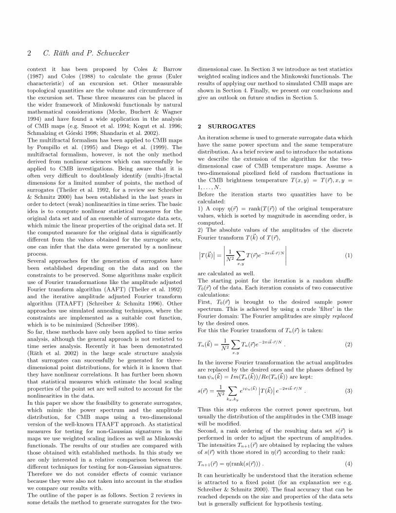
We apply the method of surrogates and weighted scalingindices to a simulated non-Gaussian CMB map, which isa realization of 12.8 deg2 CMB anisotropies due to theKayser-Stebbin effect from cosmic strings (e.g. Bouchet,Bennett& Stebbins 1988). Topological defects, althoughnot the main source of cosmic structure, are predictedin many particle physics models and are thought to beresponsible for the formation of cosmic strings at the endof an inflationary period. Fig. 1 (lower left image) showsa CMB anisotropy map generated by cosmic strings seenafter last scattering corresponding to secondary anisotropiesimprinted via the moving lens effect. Each infinitesimalelement of the cosmic string acts as a source of ’butterfly’-pattern whose superpositions lead to step-like discontinuitiesalong the string with a magnitude proportional to thelocal string velocity transversal to the line of sight (LOS).Therefore non-Gaussianities are induced by the step-likediscontinuities.We will test for non-Gaussianity by generating 20 surrogatemaps for the original non-Gaussian map and for maps withadditive white Gaussian noise with five different fluctuationlevels. The noise levels are chosen with rms ratio SNR =8, 4, 2, 1 and 0.5. In Fig. 2 the convergence of the algorithmas a function of the iteration steps is shown. We thereforecalculated the relative deviation ∆Ifourier of the powerspectrum at the n-th iteration step from the original powerspectrum,

∆Ifourier =

∑

kx,ky(|In(kx, ky)| − |I(kx, ky)|)

2

∑

kx,ky|I(kx, ky)|2

. (16)

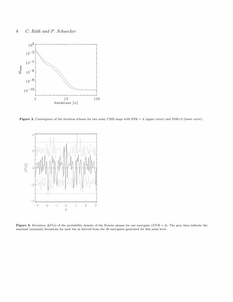
One can clearly see that the algorithm converges quickly,reproduces the original power spectrum with a very highaccuracy and saturates after approximately 30 iterationsteps. In the following all surrogates are generated using100 iteration steps.In order to test for the Gaussianity of the obtained surrogatemaps we analysed the probability density of the Fourierphases P (φ). Therefore we calculated the deviations ∆P (φ),

∆P (φ) =Psurrogate(φ)− < Prandom(φ) >

σPrandom(φ)

, (17)

of the surrogate maps from the probability densitiesPrandom(φ) of a random phase distribution. The mean <Prandom(φ) > and the standard deviation σPrandom(φ) werederived from 100 realizations of random phase distributions.Fig. 3 shows as an example the deviations ∆P (φ) for thecase SNR = 2. For most of the bins ∆P (φ) is below the 1σ-level. Only for a few uncorrelated bins the deviation becomeslarger (smaller) than 2 (−2). Therefore, no statisticallysignificant deviations from a random distribution are found.It should be noted that we did the same analysis for all othernoise levels and obtained the same results.In Fig. 1 the original (noisy) images and two respectivesurrogates are displayed. One might observe that thesurrogate maps have ’more granular’ structures but thedifferences between the original and surrogate maps arenot very pronounced, especially when the noise level isincreased. In order to quantify the structures in the imageswe calculate the spectrum of weighted scaling indices for all

maps. We normalized the temperature distribution so thatthe standard deviation σT is four at each fluctuation level.(Other normalizations are conceivable.) The radius for thecalculation of the weighted scaling indices α is chosen tor = 1.5, 2, 3, 5 and 6 pixels. The original size of the imagesand their surrogates is 256 × 256 pixels. In order to avoidedge effects we analyse only the inner part (216 × 216 pixels)of the α- and < α >-images further. Likewise, we calculatethe Minkowski functionals only for the inner part of theimages.We start the analysis of the weighted scaling indices byplotting the global means < α >global as a functionof the different radii (Fig. 4) for the original mapand the respective surrogates. Recall that the differencesbetween non-Gaussianity and Gaussianity is reflected inthe differences between the test statistics applied to theoriginal data and the surrogate data. The scatter of thesurrogates leads to measures of the statistical significance ofthe deviation between non-Gaussianity and Gaussianity. Inthe undisturbed case (Fig. 4 (a)) one finds that < α >globalfor the original map is simply shifted to lower values for allradii. This shift is due to the more ’granular-like’ structureon small scales in the surrogates. But for all images theglobal mean of the scaling indices does not change verymuch when the radius is increased. Therefore, a very gooddiscrimination between the two classes of maps (original andsurrogates) is possible for all radii. For the noisy images (Fig.4 (b) - (f) ) one finds larger variations with varying radiusand the original map is only clearly discriminable from thesurrogates until a noise level of SNR = 2 (Fig. 4 d).In Fig. 5 the global standard deviation σα of the scalingindices as a function of the different radii are shown for theoriginal map and the respective surrogates. For this globalquantity one can essentially find that for noise levels upto SNR = 1 (Fig. 5 e) one can find length scales r atwhich a discrimination between the original and surrogatesis possible.Similar discrimination results can also be obtained bycalculating the global standard deviation σ<α> of the localmeans < α > (Fig. 6). For this quantity it is remarkable thatone finds for all noise levels very different functional behaviorfor the surrogates compared to the original maps. So it isvery likely that refined analyses of the slopes and/or thecurvatures of σ<α>(r) will yield very good discriminationresults.We proceed further with a differential analyses of thescaling indices and therefore concentrate on the probabilitydensities P (α) for the (noisy) maps and their 20 surrogatesfor one value of r (r = 5) (see Fig. 7). It can clearly beseen that in the undisturbed case the differences betweenthe surrogates and the original map in the P (α) spectumare very significant, whereas the spectral differences in thenoisy cases are not so evident in this repesentation. Inorder to quantify the observed differences in the measuredprobability densities P (α) (and P (< α >) see below) wecalculate the deviation ∆P (α),

∆P (α) =Poriginal(α)− < Psurrogate(α) >

σPsurrogate(α)

, (18)

of the P (α) spectrum of the original data from themean spectrum as derived from the respective surrogatesnormalized to their standard deviation. Fig. 8 shows ∆P (α)

c© 2002 RAS, MNRAS 000, 1

Testing for primordial non-Gaussianity using surrogates 5

for all noise levels. We obtain deviations of more than 3σup to a noise level of SNR = 1. In Fig. 9 and Fig. 10 theprobability density P (< α >) and deviation ∆P (< α >) forthe local means of the scaling indices < α > are displayed.Using this quantity the differences between the surrogatesand the original maps become even more significant. Theprobability distributions in the noisy cases are broader forthe surrogates (compare also Fig. 6) and shifted to highervalues (no noise) or to lower values (high noise level).Consequently we obtain for all noise levels systematicdeviations ∆P (< α >), which have maxima for theirabsolute value, which are at least larger than 1.5σ for therespective < α >. Thus a discrimination between originaland surrogate maps seems possible up to noise levels ofSNR = 0.5.

We now compare these results with more standardmorphological analyses of temperature maps, which arebased on Minkowski functionals. Fig. 11 shows thecircumference M1 and Fig. 12 the Euler characteristic M2

for all noise levels and for the original and surrogate maps.In both cases the Minkowski functionals for the originalmap differ significantly from that for the surrogate maps upto a noise level of SNR = 1. For the Euler characteristicM2 we can also observe that there are slight systematicdifference between the original and surrogate maps in thecase of SNR = 0.5. These results are very remarkable ifthey are compared with those obtained by Chiang, Naselsky& Coles (2002). In their study they calculate Minkowskifunctionals for the same CMB map and for maps with thesame power spectrum but random phases. The authors findthat an identification of non-Gaussian signatures is onlypossible at most up to SNR = 2. In our case where boththe power spectrum and the amplitude distribution is keptone can clearly distinguish between the original map and thesurrogates even at much higher noise levels using Minkowskifunctionals. Thus we can reject the hypothesis that theCMB map is Gaussian with same power spectrum and sameintensity distribution and therefore clearly identify non-Gaussianity at high noise levels. The additional constraintof keeping the amplitude distribution leads to smallerfluctuations of the Minkowski functionals for the Gaussiansurrogate maps. Therefore, a more sensitive discriminationbetween maps with and without non-Gaussian signatures ispossible.

5 CONCLUSIONS

We have shown that it is possible to generate surrogateCMB maps which mimic both the power spectrum and theamplitude distribution of the original simulated map byapplying the method of iteratively refined surrogates.As statistical measures being sensitive to non-Gaussianitywe calculated weighted scaling indices and Minkowskifunctionals for the original and surrogate maps. For bothmeasures the values for the original data are significantlydifferent from the values obtained for the surrogate sets.Therefore a clear evidence for the non-Gaussian signaturesin the maps is given. We further tested the robustness of ourapproach with respect to white Gaussian (pixel) noise andfound that a detection of the non-Gaussianity up to SNR-

ratio of 0.5 is made possible. This result applies to both teststatistics.Comparing these results with those obtained with othertechniques (e.g. phase mapping) as proposed by Chiang,Naselsky & Coles (2002) we find that our approach issuperior concerning robustness with respect to noise. Dueto the refined construction of the surrogate maps we wereable to detect non-Gaussian signatures using Minkowskifunctionals at higher noise levels as in the above mentionedwork.So both methods the construction of amplitude adjustedsurrogates and the weighted scaling indices as an estimatorfor local scaling properties in image data turned out to beof great usefulness in the detection of non-Gaussianity inCMB-maps. Thus we obtained very promising first resultsby applying new approaches derived from nonlinear sciencesto CMB map analysis.It is likely that a more sophisticated analysis of the scalingindices will even increase the statistical significance of thediscrimination results. So the improvement of the methodsproposed in this study and their application to more realisticsimulated CMB maps incorporating mixture models as wellas to real data obtained with the WMAP- and Planck-satellites will be a rich field for future studies.

ACKNOWLEDGMENTS

The authors want to thank Milenko Zuzic and MichaelKretschmer for giving us the opportunity to discusscosmological questions in a relaxed atmosphere.

REFERENCES

Albrecht A., Steinhardt P.J., 1982, PRL, 48, 1220Barreiro R.B., Hobson M.P., 2001, MNRAS, 327, 813Bernardeau F., Uzan J.-P., 2002, astro-ph/0209330Bouchet F.R., Bennett D.P., Stebbins A., Nature, 1988, 335, 410Cayon L., Sanz J.L., Martınez-Gonzalez E., Argueso F., Gallegos

J.E., Gorski K.M., Hinshaw G., 2001, MNRAS, 326, 1243

Coles P., 1988, MNRAS, 234, 509Coles P., Barrow J. D., 1987, MNRAS, 228, 407Chiang L.-Y., Coles P., Naselsky P., 2002, astro-ph/0207584Chiang L.-Y., Naselsky P., Coles P, 2002, astro-ph/0208235Diego J.M., Martınez-Gonzalez E., Sanz J.L., Mollerach S.,

Martınez V.J., 1999, MNRAS, 306, 427Guth A. H., 1981, PRD, 23, 347

Hobson M.P., Jones A.W., Lasenby A.N., 1999, MNRAS, 309,125

Hu W., 2001, PRD, 64, 083005Julesz B., 1991, Rev. Mod. Phys., 63, 735Kogut A., Banday A.J., Bennett C.L., Gorski K.M., Hinshaw G.,

Smoot G.F., Wright E.L., 1996, ApJ, 464, L29Linde, A.D., 1982, Phys. Lett. B, 108, 389

Mataresse S., Verde L., Heavens A.F., 1997, 290, 651Mecke K., 1996, PRE, 53, 4794Mecke K., Buchert T., Wagner H., 1994, A & A, 288, 697Pompilio M.P., Bouchet F.R., Murante G., Provenzale A., 1995,

ApJ, 449, 1Rath C., Bunk W., Huber M., Morfill G., Retzlaff J., Schuecker

P., 2002, MNRAS, in press (astro-ph/0207140)

Sandvik H.B., Magueijo J., 2001, MNRAS, 325, 463Schmalzing J., Gorski K.M.,1998, MNRAS, 297, 355Schreiber T., 1998, PRL, 80, 2105

c© 2002 RAS, MNRAS 000, 1

6 C. Rath and P. Schuecker

Schreiber T., Schmitz A., 1996, PRL, 77, 635

Schreiber T., Schmitz A., 2000, Physica D, 142, 346Shandarin S.F., Feldman H.A., Xu Y., Tegmark M., 2002, ApJS,

141, 1Smoot G.F., Tenorio L., Banday A.J., Kogut A., Wright E.L.,

Hinshaw G., Bennett C.L., 1994, ApJ, 437, 1Steinhardt P. J., Turok N., 2002, astro-ph/0204479Theiler J., Eubank S., Longtin A., Galdrikian B., Farmer J.D.,

1992, Physica D, 58, 77Turok N., 1996, ApJ, 473, L5Verde L., Wang L., Heavens A.F., Kamionkowski M., 2000,

MNRAS, 313, 141Verde L., Heavens A.F., 2001, ApJ, 553, 14

c© 2002 RAS, MNRAS 000, 1

Testing for primordial non-Gaussianity using surrogates 7

Figure 1. Lowest row: Temperature map T (x, y), T ∈ [−100, 100]µK, without additive noise (left image). Some step-like discontinuitiesinducing non-Gaussianity are quite apparent. Temperature maps with additive noise: SNR = 2 (middle) and SNR = 1 (right). Upperrows: Two respective surrogate images.

c© 2002 RAS, MNRAS 000, 1

8 C. Rath and P. Schuecker

Figure 2. Convergence of the iteration scheme for two noisy CMB maps with SNR = 4 (upper curve) and SNR=2 (lower curve).

Figure 3. Deviation ∆P (φ) of the probability density of the Fourier phases for one surrogate (SNR = 4). The grey lines indicate themaximal (minimal) deviations for each bin as derived from the 20 surrogates generated for this noise level.

c© 2002 RAS, MNRAS 000, 1

Testing for primordial non-Gaussianity using surrogates 9

Figure 4. Global mean values < α >global as a function of r for the original image (black) and for the surrogates (gray). Panel (a) isfor the pure temperature map. Panel (b), (c), (d), (e) and (f) are the graphs for the combined map of CMB and additive white gaussian

noise with SNR = 8, 4, 2, 1 and 0.5, respectively.c© 2002 RAS, MNRAS 000, 1

10 C. Rath and P. Schuecker

Figure 5. Global standard deviation σα as a function of r for the original image (black) and for the surrogates (gray). Panel (a) is forthe pure temperature map. Panel (b), (c), (d), (e) and (f) are the graphs for the combined map of CMB and additive white gaussian

noise with SNR = 8, 4, 2, 1 and 0.5, respectively.c© 2002 RAS, MNRAS 000, 1

Testing for primordial non-Gaussianity using surrogates 11

Figure 6. Global standard deviation σ<α> as a function of r for the original image (black) and for the surrogates (gray). Panel (a) isfor the pure temperature map. Panel (b), (c), (d), (e) and (f) are the graphs for the combined map of CMB and additive white gaussian

noise with SNR = 8, 4, 2, 1 and 0.5, respectively.c© 2002 RAS, MNRAS 000, 1

12 C. Rath and P. Schuecker

Figure 7. Probability distribution P (α) for r = 5 for the original (black) and surrogates (gray). Panel (a) is for the pure temperaturemap. Panel (b), (c), (d), (e) and (f) are the graphs for the combined map of CMB and additive white gaussian noise with SNR = 8, 4,

2, 1 and 0.5, respectively.c© 2002 RAS, MNRAS 000, 1

Testing for primordial non-Gaussianity using surrogates 13

Figure 8. Deviation ∆P (α) of the original image from the mean surrogate distribution.Panel (a) is for the pure temperature map. Panel(b), (c), (d), (e) and (f) are the graphs for the combined map of CMB and additive white gaussian noise with SNR = 8, 4, 2, 1 and 0.5,

respectively.c© 2002 RAS, MNRAS 000, 1

14 C. Rath and P. Schuecker

Figure 9. Probability distribution P (< α >) for r = 5 for the original (black) and surrogates (gray). Panel (a) is for the pure temperaturemap. Panel (b), (c), (d), (e) and (f) are the graphs for the combined map of CMB and additive white gaussian noise with SNR = 8, 4,

2, 1 and 0.5, respectively.c© 2002 RAS, MNRAS 000, 1

Testing for primordial non-Gaussianity using surrogates 15

Figure 10. Deviation ∆P (< α >) of the original image from the mean surrogate distribution.Panel (a) is for the pure temperature map.Panel (b), (c), (d), (e) and (f) are the graphs for the combined map of CMB and additive white gaussian noise with SNR = 8, 4, 2, 1

and 0.5, respectively.c© 2002 RAS, MNRAS 000, 1

16 C. Rath and P. Schuecker

Figure 11. Minkowski functional M1 of the original image and the surrogates. The map intensities are normalized to have zero meanand a standard deviation of one. The thresholds ν are in units of the standard deviation. Panel (a) is for the pure temperature map.

Panel (b), (c), (d), (e) and (f) are the graphs for the combined map of CMB and additive white gaussian noise with SNR = 8, 4, 2, 1and 0.5, respectively. c© 2002 RAS, MNRAS 000, 1

Testing for primordial non-Gaussianity using surrogates 17

Figure 12. Minkowski functional M2 of the original image and the surrogates.Panel (a) is for the pure temperature map. Panel (b),(c), (d), (e) and (f) are the graphs for the combined map of CMB and additive white gaussian noise with SNR = 8, 4, 2, 1 and 0.5,

respectively.c© 2002 RAS, MNRAS 000, 1