Particle Accelerators, 1994, Vol. 45, pp. 1-16

Reprints available directly from the publisher

Photocopying permitted by license only

©1994 Gordon and Breach Science Publishers, S.A.

Printed in Malaysia

ANALYfICAL EVALUATION OF THE SECOND ORDERMOMENTUM COMPACTION FACTOR AND

COMPARISON WITH MAD RESULTS

J.~ SHAN, S.G. PEGGSt and S.A. BOGACZ

Fermi National Accelerator Laboratory, *, EO. Box 500, Batavia, IL 60510

(Received 27April 1992; in final form 7 March 1994)

The second order momentum compaction factor a1 is a critical lattice parameter for transition crossing inhadron synchrotrons and for the operation of quasi-isochronous storage rings. These have been proposedfor free electron lasers, synchrotron light sources and recently for high luminosity e+ e- colliders. First,the relation between the momentum compaction factor and the dispersion function is established, withthe "wiggling effect" included. Then, an analytical expression of a1 is derived for an ideal FODO lattice bysolving the differential equation for the dispersion function. A numerical calculation using MAD is performedto show excellent agreement with the analytical result. Finally, a more realistic example, the Fermilab MainInjector, is also considered.

KEY WORD: Momentum compaction, dispersion function, particle dynamics, storage rings, synchrotrons

1. INTRODUCTION

In a synchrotron or storage ring, particles with different momenta have differentclosed orbits. The difference in the closed orbit length (~C) between a particle withmomentum p and a reference particle with momentum Po may.be expressed as anexpansion in momentum offset 8

where Co is the length of the reference orbit, and

8 = P - Po = ~p.Po Po

(1)

(2)

t Now at Brookhaven National Laboratory, Upton, NY 11973.

*Operated by the Universities Research Association Inc., under contract with the U.S. Department ofEnergy.

i

2 J.P. SHAN et al.

(3)

A dependence of orbit length on momentum is called momentum compaction, and aois the linear momentum compaction factor. The second order momentum compactionfactor, aI, is the focus of this paper.

Although rooted in the transverse motion, the momentum compaction effect influ­ences the longitudinal motion through the phase slip factor,

1 T - To 2'TJ== T

o-8- =='TJO+'TJ1 8 + O(8),

where

(4)

(5)3f32 'TJo

'TJI == aOal + - - -.2')12 ')12

Here T is the period of revolution for a particle with momentum offset 8 and To is for asynchronous particle, f3 and ')I follow usual relativistic kinematic notation, and ')IT is thetransition gamma for a synchronous particle. For a conventional FODO lattice, ')IT, isroughly equal to the horizontal tune of the machine, which is about 5 I'.J 30 dependingon the size of machine. Therefore, most of the medium energy hadron synchrotronshave to cross transition. Since 8 « 1, 'TJo is the dominant contribution to 'TJ except neartransition where 'TJo is very small and the first nonlinear term

3'TJI ~ aO(al + "2) (6)

becomes very important, while the contribution from even higher order nonlinearterms can still be neglected. Nonzero 'TJI leads to the fact that higher momentumparticles and lower momentum particles can not agree when the synchronous phaseshould be switched. I In reality, the phase switch can only happen at one particularinstant, so most particles have to experience a defocusing radio frequency (rf) forcefor a period of time. This may be the dominant mechanism causing emittance blow­up and possibly beam loss for some machines, according to tracking studies2- 4 anda preliminary experiment.s If we can set al == -1.5, the nonlinear effect will besuppressed and transition crossing will become much less harmful.

All electron machines operate well above transition, or ')I » ')IT; therefore

(7)

While the bunch length is roughly proportional to yr;o, it may be possible to getvery short bunches by using quasi-isochronous rings with very small ao values. Thesehave been proposed for free electron laser drivers,6 for synchrotron light sources7

and for the next generation of high luminosity e+e- colliders.8 There, the momentumacceptance of the rfbucket, which goes roughly like 'TJO/'TJI (or all ),8,9 should be largerthan 10 times the root-mean-square (rms) momentum spread of bunch 8rms in order

SECOND ORDER MOMENTUM COMPACTION FACTOR

o

FIGURE 1: Schematic view of the wiggling effect

to preserve reasonable quantum life time. That is,

3

1al < --. (8)

108rms

If 8rms == 6 X 10-4 , a value of al smaller than 170 is required, which is not necessarilyeasy to get since ao itself is very small.

The above comments suggest that al is a very important lattice parameter which hasto be controlled in the small TJ regime. Next, we turn to establish the relation betweenthe momentum compaction factor and the dispersion function, with the "wigglingeffect" included.

2. THE WIGGLING FACTOR

To describe the closed orbit xco (s,8) of an off-momentum particle, the dispersionfunction is introduced as

D(s,8) = xco(s, 8) ~ xco(s, 0) = Do(s) + D1(s)8 + 0(82 ), (9)

where xco(s, 0) is the reference orbit, and s is the azimuthal coordinate. Usually werefer to Do, the linear part of dispersion function, as the dispersion function because8 « 1. Since we are interested in al, the first nonlinear part, D l , has also to beincluded. Furthermore, the effect of closed orbit offset on al is negligible (AppendixA), therefore we can assume xco(s, 0) == o.

4 J.~ SHAN et al.

Now, consider an infinitesimal piece of arc shown schematically in Fig. 1, where theorbit length of a synchronous particle (AA') is ds = pdf) of curvature. Then a particlewith momentum offset 8, will follow the orbit BB' with length

rather than

(11)

where Db = ~. Notice the difference between dl2 and dl l in second order, which iscalled the "wiggling effect". This relation is also valid for a straight sector if the limitp ~ 00 is taken in the appropriate way. There, the only difference in orbit length isdue to the "wiggling effect". The assumption has been made that there is no verticaldispersion.The difference in total closed orbit length of an off-momentum particle from that ofa reference particle is simply

Comparison of Equation (1) and Equation (12) yields

ao = ~ f Do ds == / Do )Co p \ p

and

al = (Ddp) + (D~2),ao 2ao

(12)

(13)

(14)

where Co = :f ds, (...) means the average in the whole ring, and the last term inEquation (14) is called the wiggling factor: IO

'21 '2 (LJo )W = 2ao (Do) = 2(Do/p)' (15)

This term is missing from some references, but will be shown to have significantcontribution to al.

Betatron oscillations may also contribute to the difference in orbit length.g,ll Thisis primarily, not a momentum dependent effect. In general, this effect is very small.

SECOND ORDER MOMENTUM COMPACTION FACTOR

3. DIFFERENTIAL EQUATIONS FOR THE DISPERSION FUNCTION

5

Motion in a circular accelerator is conveniently represented by the Hamiltonian withazimuthal coordinate s instead of time t as an independent variable

[ ]

1/2eAs x Px 2 Py 2

H = -Ps = -- - (1 + -)p 1 - (-) - (-)C P P P

eAs x [ 1 Px 2 1 (py )2]~---(l+-)p 1--(-) -- - ,

C P 2 P 2 P

where the canonical vector potential

(16)

(17)POC [x 1 x2

K 1y2 1 3 2 ]As = - - - + (- - K 1) - + -- + - K 2 (x - 3xy) ,e p p2 2 2 6

for a lattice composed of separated-function magnets with hard edge. Here K 1 andK 2 are respectively the quadrupole and the sextupole strength for a reference particle

K1

= ~ 8By K2

= ~ 82By ,

POC ax ' Poc ax2

The canonical differential equations of motion are obtained by partial differentiationof H, which expanded become

x' = 8H = (1 + ~)PX,apx p P

(18)

'2 '2)I aH 1 P - Po Po(x + Y Po 2 2

Px = -- = -Po (2: - K1)x +-- + - -K2 (x - Y ),ax p p 2p 2 (19)

where the prime represents the differentiation with respect to s, the azimuthal coor­dinate. Combining Equation (18) and Equation (19) we get the equation of motion

x" + (1 + ~ )_1_(~ _ K1)x = (1 + ~)_8_~ + x'2 + y'2 _ ~K2(X2 _ y2), (20)p 1 + 8 p2 P 1 + 8 p 2p 2

which is exact to order 82 • Substituting x = Do8 + D182 and y = 0 yields

" (1 ) 1Do + - - K 1 Do = -,p2 P

(21)

(22)

6 J.~ SHAN et al.

,,,,,\\,

R\,,

\,\,,,

QD

FIGURE 2: Schematic view of the half cell

These inhomogenous Hill equations could be solved in principle by using Green'sfunction. 12 But it is not obvious to see how the dispersion function is related to otherlattice parameters. In the next section, we will solve Equation (21) and Equation (22)explicitly for an ideal FODO lattice. This is not far away from some realistic lattices,as shown later.

4. A SOLUBLE CASE: THE IDEAL FODO LATTICE

The ideal FODO lattice that we will consider is composed of N identical FODOcells, or 2N half cells. Each half-cell (Figure 2) starts at the center of a thin focussingquadrupole (QF) and ends at the center of a neighboring thin defocussing quadrupole(QD). The absolute integrated strength of half QF and half QD is the same:

1q = IK1llhQ = 7'

where K 1 is the quadrupole gradient, and lhQ and f are respectively the physicallength and the focal length of the half quadrupole. The bending angle of each dipoleis

1r L00 == N == R'

SECOND ORDER MOMENTUM COMPACTION FACTOR 7

where L is the half cell length, or the length of each dipole since lhQ -7 0 , and R isthe radius of curvature for the reference particle. Another characteristic parameter is

s == qL ~ sin 4>1/2, (23)

which should not be confused with azimuthal coordinate s, where 4>1/2 is the betatronphase advance per half cell. It seems that one only needs to solve Equation (21) andEquation (22) in the dipole. Actually, the necessary boundary conditions also have tobe imposed by the thin quadrupoles.

In the dipole (p == Rand K 1 == 0), Equation (21) reduces to

which is equivalent to

/I 1 1DOB + R2 DoB == Ii'

DOB + DOB == R,

(24)

(25)

where a dot represents the differentiation with respect to O. The general solution ofEquation (25) is

DOB(O) == R(l + C1 sinO + C2 cosO).

In a quadrupole, Equation (22) reduces to

D~Q - K 1DoQ == 0,

which provides the boundary conditions

(26)

(27)

(31)

Here, use has been made of the symmetry condition DbQ == 0 at the center of thequadrupoles.

The continuity of D and ~~

(29)

yields

(30)

(31)

where

8

Substituting

J.~ SHAN et at.

s NsQ == Rq == - == -.

(}O 1r

DOB (()) == R(Cl cos () - C2 sin (})

(32)

(33)

into Equation (30), we arrive, after some algebra, at the solution

C2 QCl == - == (34)

Q (1+Q2)cos~·

With the aid of Equation (34), Equation (26) and Equation (33) can be rewritten as

DOB ((}) == R [1 + CI (sin () + Qcos ())] ,

DOB ((}) == RCI ( cos () - Q sin ()).

Subtituting Equation (35) into Equation (13) and Equation (15) gives

~ ()1 j+ 2 DOB 2sin T 2tQ2

ao = 00

_!!.ll. daR = 1 +C2~ = 1- 00

(1 + Q2)'2

where t == tan(~(}o), and the wiggling factor

The relationships

(35)

(36)

(37)

(38)

. () 2tSIn 0 == --2'

l+t1 - t 2

cos (}O == --2l+t

(39)

have been used to simplify the result.Following the same procedure, we now solve D 1 • In the dipole

'2/I 1 1 D OB 2 1 D OBD IB + -DIB == --(- - 1) +--

R2 R R R 2

with the general solution

DIB ((}) ==R [C3 sin () + C4 cos ()]

(40)

(41)

SECOND ORDER MOMENTUM COMPACTION FACTOR

Before solving the equation, notice

1 . 2DIB (0) == R [C3 sin 0 + C4 cos 0] - 2R DoB ,

which leads to a very simple closed result

9

(42)

(43)f+~ D 1 2 . fu1 2 IB . 2 SIn 2

aOa1 = ()O _~ d()( Ii: + 2R2 DOB ) = C4 ()O .2

To find aI, we only need to calculate C4. Let's proceed with Equation (23) in the thinquadrupole

(44)

which leads to

With Equation (31), the boundary conditions become

. 00 [00 00 D6B(±~)]D IB (±2) == -Q D IB (±2) - D OB (±2) + R .

By solving Equation (46), we find

Q4(Q2t2 + 3)C4 = 2 cos ~(1 + Q2)3'

Substituting Equation (47) into Equation (43) we have

Q4t(Q2t2 + 3)aOal == 0

0(1 + Q2)3 .

Further substitution of Equation (37) into Equation (48) allows one to write

al == (1 + Q2)2 [00(1 + Q2) _ 2tQ2] ,

which could alternatively be expressed as a function of s

(45)

(46)

(47)

(48)

(49)

(50)

Additionally, this result was independently reached through a geometric approach.13

Notice that both wand al depend only on the strength of the quadrupoles andthe number of cells. Figure 3 and Figure 4 are plots of wand al respectively as afunction of s with a different number of cells. For a given N, wand al increase as

10 J.~ SHAN et al.

Wiggling factor w in an ideal FODO lattice

1

..'..'2 ............'.............' ....'..'

4.'....'... '

.'.,'

0.2 0.4 0.6 0.8s = q*L = Half Quadrupole Strength * Half Cell Length

--....~_._-----.~.~~_.-------_._.~~~~

/~ .•., .. - - -' -_.. __..•.•.•.•.........•......I ,20·'·'·'" .•.- -

/' ,/ ...../ // 8........·...

I ,/f ,.i i

I ,./i ii i

'

I I'i

:£1.<:;::~;;~:.:: ::~::: :::::: ..'.....-.,o

o

0.6

0.5

~ 0.4\.of

9(,)

~eo 0.3.Seoeo~ 0.2

0.1

FIGURE 3: The wiggling factor w as a function of s(~sin¢ 1.) for a different number of cells in an ideal2

FODO lattice.

1

...~...

......

......

0.2 0.4 0.6 0.8s =q*L =Half quadrupole strength * Half cell length

4J}",.,

;I

I

iI'

ii

i;ii

iiii;i

,/;

i

NUlnber of cells N =infiuit..... 2iX~:·::;:;:,;:;.:::·~·~·,.·vr......----

/

,/ 8;;;;;;;;;;;ii;ii;;;;i;!

oo

1

i.6

1.4

1.2

0.8

0.6

1.8

0.4

0.2

FIGURE 4: (Xl as a function of s(~sin </> 1.) with a different number of cells in an ideal FODO lattice.2

SECOND ORDER MOMENTUM COMPACTION FACTOR 11

quadrupoles become stronger. The possible value of 8 is somewhere between 0 and1 since 8 ~ sin¢l. In the case 8 == 0 (cyclotron), from Equation (37) and Equation

2

(49) we have Qo == 1 and Ql == 0, as expected. We can show from symmetry thatQ n (n 2: 1) == O. For real synchrotrons, ¢ 1 is usually between 30 and 45 degrees, and

2

the operating range for 8 is 0.5 rv 0.7. Notice that wand Ql increase with N. SinceN increases as a factor of ring size (roughlyN ex: V"R), wand Ql are bigger for largermachines.

In the case N ~ 00, the centrifugal focusing of dipoles becomes negligible, and theanalytical results reduce to

Qo == ~ (1 _8

2

)Q2 12'

82

1 + 12W== --~-

2 (1 - ~~) ,

3(1 + ~~)Q - == 3w.

1 - 2 (1 _ ~~)

5. COMPARISON WITH MAD

(51)

(52)

(53)

In general, the differential equations cannot be solved analytically and numericalmethod has to be used. Unfortunately, Ql is not directly available from the generalcodes such as MAD,14 which instead return the momentum compaction factor Qp' Thevalue of Ql has to be extracted from the dependence of Q p on 8. Care must be takenabout which definition of Q p is used in a specific code. It may be

or

P dC [ 1 1 ] 2O:p1 = a dp = 0:0 1 + 2(0:1 + 2 - 20:0)8 +0(8 ), (54)

(55)P8 dC 2

O:p2 = as dp = 0:0(1 + 20:1 8) + 0(8 ),

or something else. It is also important to test these codes using some very simplelattices, for which an analytical solution is possible. If there is good agreement, wecan have confidence in numerical solutions of realistic lattices such as the Main RingMain Injector, or an isochronous ring.

A lattice composed of 80 simplified FODO cells was set up as input to MAD. Thelength of a quadrupole was chosen as 1 micron. For every 8, the momentum com­paction factor, Qp, is calculated by MAD at three momentum offsets,

12 J.~ SHAN et al.

1.8

1.6

1.4 +

1.2

~

Cf:JI.c0..~ 0.8

0.6

0.4

0.2

0.2 0.4 0.6 0.8 1s = q*L = I-Ialf quadrupole strength * Half cell length

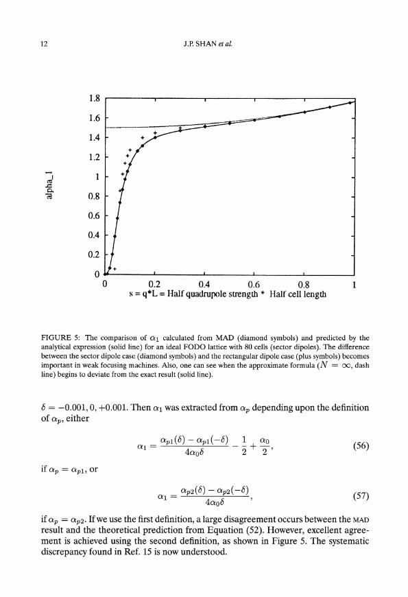
FIGURE 5: The comparison of QI calculated from MAD (diamond symbols) and predicted by theanalytical expression (solid line) for an ideal FODOlattice with 80 cells (sector dipoles). The differencebetween the sector dipole case (diamond symbols) and the rectangular dipole case (plus symbols) becomesimportant in weak focusing machines. Also, one can see when the approximate formula (N = 00, dashline) begins to deviate from the exact result (solid line).

b = -0.001,0, +0.001. Then QI was extracted from Q p depending upon the definitionof Qp, either

if Q p = Qpl, or

Qp2(8) - Qp2( -8)QI = 4Qob '

(56)

(57)

if Q p = Qp2' Ifwe use the first definition, a large disagreement occurs between the MAD

result and the theoretical prediction from Equation (52). However, excellent agree­ment is achieved using the second definition, as shown in Figure 5. The -systematicdiscrepancy found in Ref. 15 is now understood.

SECOND ORDER MOMENTUM COMPACTION FACTOR

6. DEVIATION FROM THE IDEAL FODO LATTICE

13

Taking the Main Injector (N = 80, S = sin ¥= ~) 16 as an example, we will see how

the deviations from an ideal FODO lattice affect a1.

6.1 Sector Dipoles and Rectangular Dipoles

In the ideal lattice, we assumed there was no dipole edge focusing, as with sectordipoles. In reality the Main Injector dipole is rectangular. How important is this?Figure 5 shows that the difference between sector dipoles and rectangular dipoles isnegligible in the case of Main Injector. But as the cell phase advance and/or numberof cells decreases the edge focusing becomes more important. Therefore, special carehas to be taken with edge focusing in small accelerator rings.

6.2 Finite Length Quadrupole

For the simplicity of analytical solution, we have used a thin quadrupole approxima­tion. What happens if the quadrupole has a finite length? From the MAD calculation,Table 1, we see that the contribution of finite quadrupole length is also negligible. Thisis not a surprise because the dominant source of momentum compaction comes fromdispersion in dipoles, and the boundary conditions are dominated by the integratedstrength of the quadrupoles.

TABLE 1: The dependence of a1 on the half quadrupole length

Half Quadrupole Length lQ(m) 1 x 10-6 0.1 0.5

01 1.545 1.546 1.550

6.3 Contribution from Sextupoles

Because of the head-tail instability, the natural chromaticity is usually compensatedby sextupoles. If the sextupole strengths are set to make the net chromaticity 1 - ftimes the natural chromaticity, Do (and thus ao and w) will not change while D 1 willbe modified as shown, in15

R ( 82

)(D1 ) ~ Q2 1 - f + 12 .

This approximation is true when the focussing from dipoles is negligible. Then

f 823-2 +-

a = 41 2 (1 - f~) .

(58)

(59)

14 J.~ SHAN et ale

(60)

When the net chromaticity is compensated to zero, or f == 1,

1 + 82

0.5 < al = ( 4 2) < .68,- 2 1 - f2 -

because 0 S 8 S 1. For the Main Injector 82 == 0.5, and we have al == 0.587. A value

of al == -1.5 can be obtained in principle by setting

f ~ 3,

resulting in desirably strong nonlinear fields.

7. CONCLUSION AND DISCUSSION

(61)

Starting with a Hamiltonian, we derived the differential equation for the two leadingterms in the dispersion function, which is exact for any lattice composed of separated­function magnets with hard edge. The linear term Do is determined only by linearelements (dipoles and quadrupoles). The first nonlinear correction D l also dependson sextupoles, but not on octupoles or higher order magnets.For an ideal FODO lattice, the differential equations were solved to get analyticalexpressions forao, w, and al. A comparison with MAD calculations of momentumcompaction factor showed perfect agreement. MAD was then used to show that con­ventional FODO-like lattices are not far away from the ideal one. In a large machinesuch as the Fermilab Main Injector, we found that al is not sensitive to quadrupolelength and edge focusing.

ACKNOWLEDGEMENTS

The possible importance of the previously neglected wiggling factor was first pointedout to us by Leo Michelotti. We thank K.Y. Ng for his help in the discussion ofdifferential equations. Discussions with W. Gabella were also very fruitful. Thanksalso go to C. Ankenbrandt for his comments.

REFERENCES

1. K. Johnsen, in Proceeding of the CERN Symposium on High Energy Accelerators and Pion Physics,CERN, 1956, pp.106-109.

2. J. Wei, Longitudinal Dynamics of the Non-Adiabatic Regime on Alternating-Gradient Synchrotons,Ph.D. dissertation, State University of New York at Stony Brook, May 1990.

3. S.A. Bogacz, in Proceedings ofthe Fermilab III Instabilities Workshop, (Fermilab, June 1990), p.116.

4. I. Kourbanis and K.Y. Ng, in Proceedings of the Fermilab III Instabilities Workshop, (Fermilab, June1990), pp.141-150.

5. I. Kourbanis, K. Meisner, and K.Y. Ng, in Proceedings of the IEEE Particle Accelarators Conference(San Francisco, 1991).

6. D.A.G. Deacon, Physics Report, 76, 5 (1981) 349-391.

SECOND ORDER MOMENTUM COMPACTION FACTOR 15

7. S. Chattopadhyay et aI., in Proceedings ofICFA Workshop on Low Emittance e- e+ beams, BrookhavenNational Laboratory report BNL-52090 (1987).

8. C. Pellegrini and D. Robin, Nucl. Instrum. Meth. A301 (1991) 27-36.

9. H. Bruck et aI., IEEE Trans. Nucl. Sci., 20(3):822, June 1973.

10. E. Ciapala, A. Hofmann, S. Myers, and 1: Rissela~a, IEEE Trans. Nucl. Sci., 26(3), June 1979.

11. L. Emery, in Proceedings of the 15th International Conference of High Energy Accelerators, p.1172,Hamburg, 1992.

12. J.-P. Delahaye and J. Jager, Particle Accelerators, 18:183-201, 1986.

13. K.Y. Ng, Fermilab report FN 578 (December 1991).

14. H. Grote and F.C. Iselin, The MAD Program (MethodicalAcceleratorDesign), User's Reference Manual.CERN, 8.1 edition (September 1990).

15. S.A. Bogacz and S.G. Peggs, in Proceedings of the Fermilab III Instabilities Workshop, pp.192-206,Fermilab, June 1990.

16. Fermilab Main Injector, Conceptual Design Report, Revision 2.3, appendum, Fermilab (March1991).

16 J.~ SHAN et al.

APPENDIX A. THE EFFECT OF CLOSED ORBIT OFFSET ON al

In section 2 we assume that closed reference orbit is flat, X co == O. Actually thereis always a closed orbit offset due to various errors. Since such an offset, Xco, iscomparable to D8, it is natural to ask if it will affect the calculation of al. The answeris that this effect is negligible for any realistic orbit offset.

For mathematical convenience, consider a simple model lattice, where the undis­torted closed orbit is a circle with radius R. If the distorted closed orbit for a referenceparticle is xco ( s), its circumference will be

(62)

where (x) == 2;R :f xds. The closed orbit length of a particle with momentum offset 8is

(63)

where

(64)

(65)

If Equation (63) is reorganized into an expansion of 8 with the aid of Equation (62)and compared to Equation (1), we get

(Do) + (x'D')ao == R co °

1 + (x co ) + 1(x'2)R 2 co

and

(D1) + 1 (D'2) + (x'D')al == --=-=R:....------::;:2__0 c_o_ l_

(Do) + (x'D') .R co °

(66)

Before orbit correction, the orbit offset wave has approximately the same wavelength(cell length) as the dispersion wave. The effect of closed orbit offset on al is negligibleso long as X co « Do, D I , which is always true in any practical case. After orbitcorrection the correlation between the orbit offset and the dispersion wave becomesmuch weaker, (x~oDb) and (x~oD~) average out to zero, and the condition X co «Do, Dr may not be necessary.