AN ADMISSIBLE LEVEL osp (1|2)-MODEL:MODULAR TRANSFORMATIONS AND THE VERLINDE FORMULA

JOHN SNADDEN, DAVID RIDOUT, AND SIMON WOOD

Abstract. The modular properties of the simple vertex operator superalgebra associated to the affine Kac-Moody super-algebra osp(1 |2) at level − 5

4 are investigated. After classifying the relaxed highest-weight modules over this vertex operatorsuperalgebra, the characters and supercharacters of the simple weight modules are computed and their modular transformsare determined. This leads to a complete list of the Grothendieck fusion rules by way of a continuous superalgebraic ana-logue of the Verlinde formula. All Grothendieck fusion coefficients are observed to be non-negative integers. These resultsindicate that the extension to general admissible levels will follow using the same methodology once the classification ofrelaxed highest-weight modules is completed.

1. Introduction

The construction of conformal field theories from affine Kac-Moody algebras g at fractional levels has a longhistory. These theories were first proposed by Kent [1] for g = sl (2) as a means of generalising the coset constructionof [2] to non-unitary Virasoro minimal models. Shortly thereafter, Kac and Wakimoto discovered [3] that for certainfractional levels (called the admissible levels), g possesses a finite set of simple highest-weight modules whosecharacters span, in a sense, a representation of the modular group SL(2;). It was natural then to expect thatone could build a rational conformal field theory from these highest-weight modules. However, Koh and Sorbaimmediately noticed [4] that this expectation failed, even for g = sl (2), because Verlinde’s formula [5] for the(necessarily non-negative integer) fusion coefficients always returned at least one negative number.

Subsequent work [6–15] on this observation did little to ameliorate the confusion. However, physicists eventuallyfound reason to consider modules (again for g = sl (2)) that were neither highest-weight [16–18] nor simple [19,20].Indeed, it seemed that admissible level sl (2)-theories naturally allowed for a continuously parametrised family ofsimple non-highest-weight modules, a fact that had been previously discovered [21] by Adamović and Milas.

The root cause of the negative fusion coefficients, predicted by the Verlinde formula, remained obscure untilrecently. In [22], a careful analysis of sl (2) at the admissible level k = − 1

2 showed that the negative resultscould be traced back to the fact that the simple module characters were not linearly independent. More precisely,the fundamental error in the preceding analyses was demonstrated to be that the modular transformations of thecharacters of Kac and Wakimoto did not respect their non-trivial convergence properties. Subsequent work [23–25]extended this to all admissible levels for sl (2) and proved that properly accounting for convergence regions (bytreating characters as distributions, not meromorphic functions) indeed resulted in non-negative integer fusioncoefficients. Moreover, the corresponding Grothendieck fusion rules agreed perfectly with the fusion rules that wereknown [19,26] from independent computations.

We remark that these successes were obtained as one instance of a rather more general methodology, dubbed thestandard module formalism [27, 28], for modular properties and Verlinde-like formulae in logarithmic conformalfield theories. Originating in work on theories based on the affine Kac-Moody superalgebra gl (1|1) [29–31], thisformalism has since been applied to a wide range of logarithmic conformal field theories [32–40], all of which arein some sense related to rank 1 objects such as the A1 lattice.

There is therefore a need to explore higher rank logarithmic conformal field theories and the standard moduleformalism is expected to be crucial to this endeavour. The analysis of higher rank theories constructed from affineKac-Moody algebras (and superalgebras) at admissible levels is particularly attractive because we expect that theywill play a central role in understanding logarithmic models, just as the Wess-Zumino-Witten models do in the

2010 Mathematics Subject Classification. Primary 17B69, 81T40; Secondary 17B10, 17B67.

1

2 J SNADDEN, D RIDOUT, AND S WOOD

rational case. However, this analysis is still in its infancy. The relevant simple highest-weight modules have beenidentified by Arakawa [41] for all admissible levels, but a complete set of (positive-energy) simple modules has onlyrecently been described for sl (3) [42]. More generally, almost nothing is known aside from some partial level-specificresults for affine algebras [43–49] and superalgebras [50–57].

In this paper, we shall not embark immediately on a study of higher rank logarithmic conformal field theories.Rather, we will describe in detail a particular example based on the affine Kac-Moody superalgebra osp(1|2) atthe admissible level k = − 5

4 . The aim here is to develop and test the standard module formalism in the presenceof fermionic degrees of freedom (and determine the precise role of the Ramond sector) before tackling the morechallenging, but also more physically interesting, cases of sl (2|1) and psl (2|2).1 This particular level is an attractivestarting place for two reasons: first, it describes one of the “smallest” osp(1|2) minimal models (meaning that it hasvery few simple highest-weight modules) and, second, it is an order 2 simple current extension of the sl (2) minimalmodel of the same (admissible) level [25]. The latter property allows us to independently check our osp(1|2) resultsagainst the known sl (2) results.

Of course, conformal field theories with osp(1|2) symmetry have been studied in the past, both at integer andfractional levels [58–60]. However, these works only considered simple highest-weight modules in the Neveu-Schwarz (untwisted) sector, ignoring the known issue of negative fusion coefficients. Here, we discuss a morecomplete spectrum of simple modules (as well as some of the reducible but indecomposable ones) in both theNeveu-Schwarz and Ramond sectors. We moreover emphasise the global parity of each module in order to beable to distinguish the relative parities of the direct summands appearing in each Grothendieck fusion product. Inphysics parlance, this is equivalent to computing both the even and odd Grothendieck fusion rules of Sotkov andStanishkov [61].

The results confirm that the standard module formalism applies to the affine superalgebra theory studied here:characters and supercharacters close under modular transformations and the Grothendieck fusion coefficients areverified to be non-negative integers. The methodology developed in this paper also applies to the other admissiblelevels of osp(1|2), so extending these results to general admissible levels will be straightforward, assuming that onecan first classify the relaxed highest-weight modules. The latter classification has not yet been completed, thoughwe expect that it can be obtained using the methods developed in [62–65]. Because of this, the Grothendieck fusionrules of the osp(1|2) models for general admissible levels will instead be addressed in a forthcoming paper [66] usingcoset technology. A byproduct of this work will be the relaxed highest-weight module classification for osp(1|2)models of general admissible level.

We begin, in Section 2, with a quick review of the simple Lie superalgebra osp(1|2) and its representation theory.We prove, in particular, a classification result (Theorem 2) for all simple weight modules of osp(1|2) that have at leastone finite-dimensional weight space (wewere unable to find this result in the literature). This is followed, in Section 3,by a quick review of the affine Kac-Moody superalgebra osp(1|2), its automorphisms (conjugation and spectral flow),and the associated vertex operator superalgebras. We also discuss relaxed Verma modules over osp(1|2) and theirsimple quotients, borrowing this notion from [16] where it was introduced for sl (2) (see [64, Sec. 2.1] for a generaldefinition of relaxed highest-weight modules).

Section 4 then specialises to the simple osp(1|2) vertex operator superalgebra of level k = − 54 that we study

in this work, denoting it by B0 |1 (2, 4). We first give an efficient characterisation of affine Zhu algebras, twistedand untwisted, and identify those of the universal vertex operator superalgebras (Proposition 6) before explicitlycomputing the Zhu algebras of B0 |1 (2, 4) (Propositions 7 and 8). This is then used to classify the simple relaxedhighest-weightB0 |1 (2, 4)-modules (Theorems 9 and 10) and identify some of the reducible ones. These are partitionedinto standard, typical and atypical modules as per the standard module formalism of [27, 28].

1We mention that the corresponding analysis for the gl (1 |1) logarithmic conformal field theory, carried out in [29], was restricted to the Neveu-Schwarz sector as the simple characters of this sector closed on themselves under modular transformations. The same is not true for osp(1 |2)conformal field theories.

3

Having classified the simple (and standard) B0 |1 (2, 4)-modules, we turn to the computation of their charactersand supercharacters in Section 5. Such character formulae are easy to compute for the Neveu-Schwarz highest-weight modules because the submodule structure of the associated Verma modules was determined by Iohara andKoga [60]. Spectral flow automorphisms then allow us to deduce the analogous Ramond formulae (Proposition 11).We explicitly note the convergence regions of these characters, treated as meromorphic functions, and use the resultsto determine the characters of the relaxed highest-weight modules, treated as distributions (Propositions 12 and 13).Supercharacter formulae follow easily (Proposition 14) and we conclude by introducing the Grothendieck group of(an appropriate category of) B0 |1 (2, 4)-modules and showing explicitly that the images of the standard modules forma basis of (a completion of) this Grothendieck group.

This last result (Corollary 16) is the key to computing the modular transforms of the B0 |1 (2, 4)-(super)characters,the topic of Section 6. We begin by introducing slightly unfamiliar S and T coordinate transforms (following [35])before computing the modular group action on the span of the standard B0 |1 (2, 4)-(super)characters. Of note is thatthe S-transform amounts to a generalised Fourier transform on (a countably-infinite number of copies of) the realvector space h spanned by the fundamental weight of osp(1|2). The S-transforms are then extended to the simpleatypical (super)characters using Corollary 16. We remark that trying to compute these S-transforms directly from themeromorphic characters would lead to nonsensical results (such as negative fusion coefficients) because the modularS-transform does not preserve the convergence regions of the (super)characters.

Finally, Section 7 addresses the Grothendieck fusion rules of the simple (and standard) B0 |1 (2, 4)-modules. First,we deduce a version (Theorem 21) of the standard Verlinde formula that works for this vertex operator superalgebra— generally, Verlinde formulae are only expected to apply directly to (-graded) vertex operator algebras. Themethod follows the approach of [67] for the N = 1 minimal model vertex operator superalgebra (see also [39])wherein one lifts the Verlinde formula from the bosonic orbifold using simple current technology. With this formulain hand, we compute all Grothendieck fusion rules, including global parity information, among the simple andstandard B0 |1 (2, 4)-modules (Theorem 25).

Acknowledgements

DR thanks Kenji Iohara for illuminating discussions on the structure of Verma modules over osp(1|2). Wewould like to thank the anonymous referee whose careful reading of the original manuscript and many suggestionssignificantly improved the article. JS’s research is supported by a University Research Scholarship from theAustralian National University. DR’s research is supported by the Australian Research Council Discovery ProjectsDP1093910 and DP160101520 as well as the Australian Research Council Centre of Excellence for Mathematicaland Statistical Frontiers CE140100049. SW’s research is supported by Australian Research Council Discovery EarlyCareer Researcher Award DE140101825 and the Australian Research Council Discovery Project DP160101520.

2. The basic Lie superalgebra osp(1|2)

In this section, we quickly review the theory of weight modules over sl (2) and osp(1|2). The latter algebra isimportant because of its role as the horizontal subalgebra of the Neveu-Schwarz osp(1|2) algebra, the former playsthe same role for the Ramond osp(1|2) algebra.

2.1. A brief review of sl (2). The simple complex Lie algebra A1 = sl (2) has Cartan-Weyl basis h, e, f , satisfyingthe commutation relations

[h, e] = 2e, [h, f ] = −2f , [e, f ] = h. (2.1)

The Cartan subalgebra h = h then gives rise to the root system α ,−α ⊂ h∗ where α (h) = 2 and we choose α tobe the lone fundamental root. The non-zero entries of the (appropriately normalised) Killing form κ on sl (2), withrespect to the given basis, are

κ (h,h) = 2, κ (e, f ) = κ ( f , e ) = 1. (2.2)

4 J SNADDEN, D RIDOUT, AND S WOOD

This induces an inner product on h∗, defined by (α , α ) = 2. From these data, one calculates the fundamental weightto be ω = 1

2 α and that the algebra has dual Coxeter number h∨ = 2. The Weyl group is isomorphic to 2, generatedby the root reflection α 7→ −α .

As with all complex semisimple Lie algebras, the finite-dimensional modules of sl (2) are necessarily semisimpleweight modules and the finite-dimensional simple modules are uniquely determined (up to isomorphism) by theirhighest weight. For eachλ ∈ ≥0, we denote the unique (up to isomorphism) (λ+1)-dimensional simple sl (2)-moduleof highest weight λω (and lowest weight −λω) by Fλ .

Extending to the infinite-dimensional case, we no longer have complete reducibility, though we can neverthelessclassify the simple weight modules. Here we include in the definition of a weight module that all of its weightspaces are required to be finite-dimensional. The first class that we consider are the simple highest-weight modulesD+

λ , where λ ∈ \ ≥0, with highest weight λω and no lowest weight. It is straightforward to show that the weightsupport (the set of weights with non-trivial weight spaces) of such a module is (λ − 2≥0)ω and that all the weightspaces are one-dimensional. Similarly, we also have the simple lowest-weight modulesD

−

λ where λ ∈ \≤0. Here,the weight support is instead (λ + 2≥0)ω and again all weight spaces are one-dimensional.

Finally, we have the dense modules EΛ,q , parametrised by q ∈ and Λ ∈ /2. These are simple preciselywhen q , 1

2λ(λ + 2) for all λ ∈ Λ. The weight support of EΛ,q is precisely Λω (that is, (λ0 + 2)ω for some λ0),again with all weight spaces one-dimensional. The parameter q is the (unique) eigenvalue of the Casimir elementQ = 1

2h2 + e f + f e which generates the centre of the universal enveloping algebra and must therefore act as a

scalar multiple of the identity. We remark that dense modules are also referred to as cuspidal and torsion-free in theliterature.

Having introduced the above classes of modules, we can state the following result (see [68]).

Theorem 1 (Classification of simple sl (2) weight modules). Every simple sl (2) weight module is isomorphic to oneof the following mutually non-isomorphic modules:

(i) Fλ with λ ∈ ≥0;(ii) D

+

λ with λ ∈ \ ≥0;(iii) D

−

λ with λ ∈ \ ≤0;(iv) EΛ,q with q ∈ , Λ ∈ /2 and q , 1

2λ(λ + 2) for all λ ∈ Λ.

We shall also need to consider the reducible, but indecomposable, dense modules that correspond to parametersΛ and q, where q = 1

2λ(λ + 2) for some λ ∈ Λ. We note that these do not exhaust the reducible but indecomposabledense modules of sl (2). The latter are classified (somewhat explicitly) in [68]. However, the others will not beneeded in what follows. If this condition is met, then either the unique (up to rescaling) state vλ of weight λω isa highest-weight vector or evλ is a lowest-weight vector. Both possibilities occur independently:2 the first givesrise to a highest-weight submodule isomorphic to the highest-weight module D

+

λ , while the second gives rise to alowest-weight submodule isomorphic to the lowest-weight module D

−

λ+2. The structures of these indecomposabledense sl (2)-modules, which we denote by E

+

Λ,q and E−

Λ,q , respectively, where Λ = λ + 2, are thus determined bythe following non-split short exact sequences:

0 −→ D+

λ−2 −→ E+

λ+2,λ (λ−2)/2 −→ D−

λ −→ 0, 0 −→ D−

λ+2 −→ E−

λ+2,λ (λ+2)/2 −→ D+

λ −→ 0. (2.3)

We have shifted λ by 2 in the first sequence for clarity.We recall a concrete construction of certain dense sl (2)-modules that will be useful when we generalise to

dense osp(1|2)-modules in Section 2.2. First, note that the elements of the universal enveloping algebra whichcommute with h ∈ sl (2) (more generally, with the Cartan subalgebra) will preserve weight spaces. Such elementsform the centraliser C(h,U(sl (2))), which (by the Poincaré-Birkhoff-Witt theorem) is just the polynomial subalgebra[h,Q] ⊆ U(sl (2)). As this is abelian, its simple modules are all one-dimensional. Suppose that Wλ,q = w is one

2We assume throughout that when λ solves the reducibility condition, then it is the unique element of Λ that does so. This need not be the case,as for certain q there are two solutions for λ in Λ. However, the corresponding reducible modules will, again, not be needed here.

5

such module, with h and Q acting as complex scalars λ and q, respectively. We can then induce from this to the fullU(sl (2))-module

Wλ,q = IndU(sl (2))C(h,U(sl (2))) Wλ,q , (2.4)

which (again using the Poincaré-Birkhoff-Witt theorem) has basis

w, enw, f nw : n ∈ >0. (2.5)

The induced moduleWλ,q obviously has weight support Λω, where Λ = λ+2, and one-dimensional weight spaces,hence it is dense. It is moreover clear that Wλ,q is a simple sl (2)-module, and is thus isomorphic to EΛ,q , unlessenw is a lowest-weight vector or f nw is a highest-weight vector, for some n ∈ >0. When Wλ,q is not simple, it isisomorphic to E

−

Λ,q or E+

Λ,q , respectively.

2.2. A brief review of osp(1|2). The simple complex Lie superalgebra g = osp(1|2) has basis h, e, f ,x ,y, wherethe elements of g(0) = span h, e, f and g(1) = span x ,y are declared to be even and odd, respectively. The evensubalgebra is (as its elements suggest) isomorphic to sl (2), thus (2.1) still holds. The remaining (anti)commutationrelations are:

[h,x] = x , [e,x] = 0, [f ,x] = −y,

[h,y] = −y, [e,y] = −x , [f ,y] = 0,

x ,y = h, x ,x = 2e, y,y = −2f .

(2.6)

In this basis, the (rescaled) Killing form has non-zero entries given by

κ (h,h) = 2, κ (e, f ) = κ ( f , e ) = 1, κ (x ,y) = −κ (y,x ) = 2. (2.7)

Due to the existence of a non-degenerate even supersymmetric bilinear form, osp(1|2) is an example of a basic Liesuperalgebra [69]. In the classification [70] of such algebras, the isomorphism class of osp(1|2) is denoted by B0 |1.

We consider the Cartan subalgebra h = h, with root system −2α ,−α ,α , 2α, where α (h) = 1 (so 2α is identifiedwith α), and choose α to be positive (hence simple). The inner product on h∗ induced by the Killing form is given by(α ,α ) = 1

2 , from which one can calculate that the dual Coxeter number is h∨ = 32 and that the fundamental weight is

α . Since the Weyl group of a Lie superalgebra is generated by reflections in the even roots, it is precisely the Weylgroup of its even subalgebra. As the even subalgebra of osp(1|2) is isomorphic to sl (2), its Weyl group is also oforder 2, generated by the reflection α 7→ −α .

As with all superalgebras, modules M of osp(1|2) are required to carry a compatible 2-grading: that is, theymust decompose as a direct sumM(0) ⊕M(1) , such that g(i )M(j ) ⊆ M(i+j ) , for all i, j ∈ 2. Having identified such anM(0) andM(1) , these summands are then referred to as the even and odd subspaces, respectively. Similarly, elementsof the even and odd subspaces are said to have even and odd parity, respectively. However, it should be apparentthat reversing these labels, whilst maintaining the same module structure, still gives a valid grading. As such, onany category of modules we might consider, we require there to be an involutive functor Π taking any module to itsparity reversal. In principle, a module may be isomorphic to its parity reversal. This does not happen for the simpleweight modules of osp(1|2).

All finite-dimensional osp(1|2)-modules are semisimple weight modules. The simple ones must have a uniquehighest (and lowest) weight. Indeed, for each λ ∈ ≥0, there is a unique (up to isomorphism) (2λ + 1)-dimensionalsimple osp(1|2)-module with highest weight λα and lowest weight −λα , for which the highest-weight vectors (andthus also the lowest-weight vectors) are assigned even parity. We will denote this module by Aλ . It has weightsupport µα : µ ∈ , |µ | ≤ λ, with all weight spaces one-dimensional.

In addition, for each λ ∈ \ ≥0, osp(1|2) has an infinite-dimensional simple highest-weight module B+

λ ,generated by an even highest-weight vector of weight λα , whose weight support is (λ − ≥0)α . Similarly, there isalso the simple lowest-weight module B

−

λ , for each λ ∈ \≤0. This module is generated by an even lowest-weightvector of weight λα and its weight support is (λ + ≥0)α .

6 J SNADDEN, D RIDOUT, AND S WOOD

The modules listed above, together with their parity reversals, exhaust the simple highest- and lowest-weightmodules of osp(1|2). The proof is elementary, following the same steps used to classify highest-weight sl (2)-modules. Moreover, again as with sl (2), there is an additional infinite family of simple weight modules with nohighest nor lowest weights. However, a little care is needed here to characterise these in a meaningful way.

Recall from Section 2.1 the concrete construction of certain dense sl (2)-modules. For g = osp(1|2), the centre ofthe universal enveloping superalgebra U(g) is still generated by a Casimir element

Q ′ =12h2 + e f + f e −

12xy +

12yx , (2.8)

which must therefore act as a scalar on any simple module, but the centraliser C(h,U(osp(1|2))) is not a polynomialalgebra in h and Q ′. For example, by rewriting the previous equation in the form

Q ′ =12h2 +

12h − yx + 2(yx )2 − 2h(yx ), (2.9)

we see that yx cannot be expressed as a polynomial in these elements, though indeed (yx )h = h(yx ).This motivates introducing the super-Casimir (or sCasimir) [71]

Σ = xy − yx +12∈ C(h,U(osp(1|2))). (2.10)

Though this element of U(g) is not central, it satisfies

[Σ, g(0)] = Σ, g(1) = 0, (2.11)

from which it follows that Σ is diagonalisable on a simple weight module, taking eigenvalues s and −s on the evenand odd subspaces, respectively, for some s ∈ . We can now identify C(h,U(osp(1|2))) with the polynomial algebra[h, Σ]. In particular, we may write yx and Q ′ as polynomials in h and Σ as follows:

yx =12

(h − Σ +

12

), Q ′ =

12Σ2 −

18. (2.12)

We note that the eigenvalue of Σ is λ + 12 on a highest-weight vector of weight λα and −λ + 1

2 on a lowest-weightvector of the same weight. As mentioned above, this eigenvalue is denoted by s if the highest-/lowest-weight vectoris even and −s if it is odd.

One can carry out an induction procedure analogous to that described by (2.4), giving weight g-modules W′

λ,s

with basesw,xnw,ynw : n ∈ >0, (2.13)

where hw = λw and Σw = sw , for some λ, s ∈ , assigning even parity to w . As in the sl (2) case, this is a densemodule: its weight support is λ + and its weight spaces are one-dimensional.

W′

λ,s is reducible if and only if it has either a highest- or a lowest-weight vector, thus if one of the basis elementsabove is annihilated by either x or y. If s = µ + 1

2 , for some µ ∈ λ + 2 (so that the corresponding weight vector vµhas even parity), then either vµ is a highest-weight vector or xvµ is a lowest-weight vector. Similarly, if s = −µ + 1

2 ,for some µ ∈ λ + 2, then either vµ is a lowest-weight vector or yvµ is a highest-weight vector.3 If neither constraintis satisfied, that is if µ2 , (s − 1

2 )2 for every µ ∈ λ+ 2, thenW

′

λ,s is simple. In this instance, we can unambiguouslylabel these simple dense modules as CΛ,s , where Λ = λ + 2, in analogy with the notation used for simple densesl (2)-modules. Clearly, CΛ,s has weight support (Λ + 0, 1)α and Σ acts as (−1) js on weight vectors whose weightslie in (Λ + j )α . We also note the isomorphisms

CΛ,s ΠCΛ+1,−s . (2.14)

This argument shows that the simple weight modules are classified in a manner entirely analogous to Theorem 1.In particular we have:

3The analogous analysis in which vµ has odd parity leads to equivalent constraints on s .

7

Theorem 2 (Classification of simple osp(1|2) weight modules). Every simple osp(1|2) weight module is isomorphicto one of the following mutually non-isomorphic modules, or their parity reversals:

(i) Aλ with λ ∈ ≥0;(ii) B

+

λ with λ ∈ \ ≥0;(iii) B

−

λ with λ ∈ \ ≤0;(iv) CΛ,s with s ∈ , Λ ∈ /2 and λ2 , (s − 1

2 )2 for every λ ∈ Λ.

Proof. Let M be a simple weight module over osp(1|2) and suppose that w ∈ M is a vector of weight λα so thathw = λw . If the even subspace of M is zero, then w is odd and both xw and yw vanish, so that M = w ΠA0.Otherwise, without loss of generality, we may assume thatw is of even parity.

Simplicity implies that M = U(g)w and, in particular, that the weight space of weight λα is

M(λ) = C(h,U(osp(1|2)))w . (2.15)

Now, ifM(λ) had aC(h,U(osp(1|2)))-submodule, then this would generate a proper g-submodule ofM, contradictingits simplicity. It therefore must be that M(λ) is a simple C(h,U(osp(1|2)))-module and, since C(h,U(osp(1|2))) isabelian, M(λ) is thus one-dimensional. It follows that w is an eigenvector of Σ with, say, Σw = sw and, by thePoincaré-Birkhoff-Witt theorem, M is spanned by

w,xnw,ynw : n ∈ >0. (2.16)

By iterative application of the (anti)commutation relations (2.6), one can uniquely determine the action of anyelement of g onM in terms of the parameters λ and s. If the spanning set (2.16) is linearly dependent, thenMmust behighest- and/or lowest-weight and thus belongs to classes (i), (ii) or (iii), as discussed above. OtherwiseM W

′

λ,s ,so it belongs to class (iv).

Whilst all finite-dimensional osp(1|2)-modules are semisimple and can therefore be decomposed into a directsum of a finite number of the Aλ and ΠAλ , there are infinite-dimensional modules which are not. In particular, thedense moduleW

′

λ,λ+1/2 is reducible, but indecomposable, and is characterised by the following non-split short exactsequence:

0 −→ ΠB−

λ+1 −→W′

λ,λ+1/2 −→ B+

λ −→ 0. (2.17a)

We shall denote this reducible moduleW′

λ,λ+1/2 by C−

Λ,s , whereΛ = λ+2 and s = λ+ 12 , to emphasise its denseness.

The superscript − refers to the existence of a lowest-weight submodule. Indeed, one similarly arrives at the non-splitshort exact sequence

0 −→ ΠB+

λ−1 −→W′

λ,−λ+1/2 −→ B−

λ −→ 0 (2.17b)

in an entirely analogous manner. We therefore denote W′

λ,−λ+1/2 by C+

Λ,s , where Λ = λ + 2, s = −λ + 12 and the

superscript + indicates a highest-weight submodule.It will turn out, in Section 4, that these reducible, but indecomposable, modules are the keys to the analysis of the

conformal field theory. We remark that if s ∈ + 12 \ 1

2, then the indecomposable structure of the induced moduleW′

λ,s is slightly more complicated that that discussed above. However, this case turns out not to be relevant for theconformal field theory that we shall explore, hence it will not be considered any further. There are, in addition, manyother indecomposable dense osp(1|2)-modules beyond those discussed here which are likewise irrelevant to whatfollows.

2.3. TheWeyl group. Although we have, in both Sections 2.1 and 2.2, treated the Weyl group W(h) associated witha chosen Cartan subalgebra as the subgroup of GL(h∗) generated by (even) root reflections, it is possible (and useful)to view it in a number of other ways. One equivalent definition (for any simple Lie superalgebra g with Cartansubalgebra h) is

W(h) =N(h)

Z(h), (2.18)

8 J SNADDEN, D RIDOUT, AND S WOOD

where N(h) and Z(h) are the subgroups of the group Inn(g) of inner automorphisms of g given by

N(h) = ϕ ∈ Inn(g) : ϕ (h) = h, Z(h) = ϕ ∈ Inn(g) : ϕ (x ) = x for all x ∈ h. (2.19)

We recall that for a simple Lie superalgebra, the group of inner automorphisms is generated by exponentiating theadjoint actions of the even subalgebra elements. Now, if the quotient (2.18) splits, so that

N(h) = Z(h) o W(h), (2.20)

then we may treat the Weyl group as a subgroup of Inn(g); in particular, one which preserves the choice of Cartansubalgebra.

For example, for the Cartan subalgebra h of sl (2) used in Section 2.1, N(h) is the union of two disjoint subsets:those maps taking h 7→ h and those taking h 7→ −h. The first is of course Z(h), so taking the quotient as in (2.18)indeed gives a copy of the Weyl group 2. A choice of coset representatives are the identity map idg and the linearinvolution defined by

h 7→ −h, e 7→ −f , f 7→ −e, (2.21)

demonstrating the splitting (2.20).Now, for osp(1|2), with h as in Section 2.2, we again find that Z(h) is a normal subgroup of N(h) of index 2,

so that indeed the Weyl group is isomorphic to 2. However, this quotient no longer splits. We can see this byagain considering coset representatives. Here, we may choose these to be the identity map and the conjugationautomorphism w, which acts according to (2.21) on the even subalgebra and on odd elements as

wx = −y, wy = x . (2.22)

Note that w is not involutive, but rather squares to an element 1 ∈ Z(h) which acts as the identity on even elementsand minus the identity on odd ones. Indeed, no element of that coset squares to the identity, so unfortunately wecannot here realise the Weyl group as a subgroup of Inn(g).

It is also useful to consider automorphisms of g as defining invertible functors on the categoryModg of g-modules.Taking any φ ∈ Aut(g) and anyM ∈ Modg, let φ : M→ φM be an isomorphism of vector superspaces and let X ∈ gact on φ (m) ∈ φM according to

X φ (m) = φ (φ−1 (X )m). (2.23)

This gives φM the structure of a g-module. We emphasise that φM may or may not be isomorphic to M. Theassignment M 7→ φM is called twisting by φ and indeed defines a functor on the category of g-modules (acting inthe obvious way on morphisms). The resulting homomorphism Aut(g) −→ Aut(Modg ) is then a strict Aut(g)-actionon Modg. These functors obviously commute with parity reversal: Πφ = φΠ. For notational simplicity, we shalldrop the tildes that distinguish the automorphism from its induced functor in what follows.

Two notable properties of these twisting functors are that they preserve indecomposable structures and take weightmodules to weight modules, albeit with respect to possibly different Cartan subalgebras. Indeed, if M is a weightmodule for h, then φ (h) is another Cartan subalgebra for which φM is a weight module. However, since all Cartansubalgebras are related to one another by inner automorphisms, we are justified in restricting attention to φ ∈ N(h)

for a given h. Moreover, twisting by φ ∈ Z(h) takes (isomorphism classes of) weight modules to themselves, thus weneed only consider those twists defined (up to isomorphism) by the cosets in W(g). We have, in this way, obtainedan action of the Weyl group on the set of isomorphism classes of the objects of WModg, the category of weightg-modules (with fixed Cartan subalgebra h). In general, one can also act with (equivalence classes of) those outerautomorphisms that preserve the chosen Cartan subalgebra. However, for sl (2) and osp(1|2), there are no such outerautomorphisms.

We illustrate this action of the Weyl group with the following two examples. If g = sl (2) and φ is the innerautomorphism defined in (2.21), then we have

φFλ Fλ , φD±

λ D∓

−λ , φEΛ,q E−Λ,q . (2.24a)

9

Similarly, for osp(1|2) we have

wAλ Aλ , wB±

λ B∓

−λ , wCΛ,s C−Λ,s . (2.24b)

Note that in these examples, the induced action on the weight support of the module is precisely that of thecorresponding Weyl reflection. This generalises, with the twisting functor corresponding to a Weyl group elementacting on a module’s weight support via its standard linear action on the dual Cartan subalgebra.

We remark that it is possible to lift the action of the Weyl group from isomorphism classes of weight modulesto the category WModg. This is trivial for g = sl (2), because of (2.21), but not for g = osp(1|2) as w2 , 1.In the latter case, we instead have natural isomorphisms ηM : w2

M → M, for each weight module M, given byηM

(w2 (m)

)= (−1) |m |m, for all homogeneous elements m ∈ M. Here, |m | ∈ 0, 1 denotes the parity of m. It

is now easy to check that these natural isomorphisms, along with the identity, satisfy the associativity constraintsrequired to give WModosp(1 |2) a Weyl group action. However, this action is not essential for much of the analysis tofollow because we will be chiefly concerned with identifying weight modules up to isomorphism.

3. The affine Kac-Moody superalgebra osp(1|2)

We now turn to the affinisation osp(1|2) in its Neveu-Schwarz and Ramond guises as well as the associatedvertex operator superalgebras. Verma modules and their generalisations, the relaxed Verma modules, are introducedalong with their simple quotients. The conjugation and spectral flow automorphisms are used to twist the latterand thereby construct a large collection of simple smooth weight modules over osp(1|2), almost none of which arepositive-energy. We recall that a module being smooth means that for all j ∈ osp(1|2) and v in the module, jm · vvanishes form sufficiently large (see below for notation).

3.1. The affine algebra. The affineKac-Moody superalgebra osp(1|2)may be defined, as a vector space, by choosinga basis. The standard choice is

hm , em , fm : m ∈ ∪ xm ,ym : m ∈ + ξ ∪ K ,L0, (3.1)

where ξ is either 0 or 12 , giving what we will call the Neveu-Schwarz and Ramond osp(1|2) algebras, gNS and

gR, respectively. As we will demonstrate later, these two choices of indexing give isomorphic algebras, hence wewill generally suppress the subscripts and just write g = osp(1|2). However, many of the representation-theoreticconstructions that we shall consider depend on this choice. In particular, the representation theory splits into twosectors according to which algebra, Neveu-Schwarz or Ramond, is acting on the module. The modules on which gNS

acts constitute the Neveu-Schwarz sector and the gR-modules constitute the Ramond sector.In both cases, the even subalgebra is defined to be spanned by the hm , em and fm , as well as K and L0. The

xm and ym are declared to be odd. Letting j, j ′ ∈ h, e, f ,x ,y denote arbitrary basis vectors of osp(1|2), the(anti)commutation relations of the affine basis vectors (3.1) take the form

[jm , j ′n] = [j, j ′]m+n +mκ (j, j ′)δm+n,0K if j or j ′ is even,

jm , j ′n = j, j ′m+n +mκ (j, j ′)δm+n,0K if j and j ′ are odd,[L0, j

′n] = −nj ′n (3.2)

and K is central. We recall that the (anti)commutators of the basis elements of osp(1|2) were given in (2.1) and (2.6),while the non-zero values taken by the (normalised) Killing form were listed in (2.2) and (2.7).

Note that the Neveu-Schwarz algebra gNS has a finite-dimensional subalgebra spanned by h0, e0, f0,x0,y0,isomorphic to osp(1|2). This is the horizontal subalgebra of gNS. The inclusion allows us to carry much of therepresentation-theoretic data we have for osp(1|2) over to osp(1|2). The horizontal subalgebra of the Ramond algebragR is defined instead to be spanned by h0, e0, f0 (because odd elements do not have zero modes in gR), hence it isisomorphic to sl (2). Our study of the Ramond sector will therefore be closely related to sl (2) representation theory.

The Cartan subalgebra h of both gNS and gR is defined to be the abelian subalgebra spanned by h0, K and L0. Withrespect to h, these algebras have root systems

±2α + nδ : n ∈ ∪ ±α + nδ : n ∈ + ξ ∪ nδ : n ∈ ,0, (3.3)

10 J SNADDEN, D RIDOUT, AND S WOOD

where the roots α ,δ ∈ h∗ are defined by

α (h0) = 1, α (K ) = α (L0) = 0,

δ (h0) = δ (K ) = 0, δ (L0) = −1.(3.4)

The positive roots are taken to be those in (3.3) with n > 0, along with α and 2α . The simple roots are thenα ,−2α +δ in the Neveu-Schwarz case and 2α ,−α + 1

2δ in the Ramond case. These choices of simple roots giverise to identical generating reflections for the Weyl group.

3.2. Generalised Verma modules and vertex operator superalgebras. Given the choice of positive roots above,we obtain triangular decompositions for g = gNS and gR:

g = g− ⊕ h ⊕ g+. (3.5)

Here, g+ and g− denote the subalgebras of g spanned by the positive and negative root vectors, respectively. Forexample, g+NS is spanned by x0, e0 and all the jm , j = e,x ,h,y, f , withm ∈ >0. Associated with each decompositionis the Borel subalgebra b = h ⊕ g+.

We define a weight space of an osp(1|2)-module to be a simultaneous eigenspace of h0 and K that is alsoa generalised eigenspace of L0. We then define a weight module over osp(1|2) to be a 2-graded module thatdecomposes (as a vector space) into a direct sum of finite-dimensional weight spaces. Note that although L0 ispermitted to act non-semisimply on a weight module, its Jordan blocks will have finite rank.

Consider now a one-dimensional b-module spanned by some v , 0 on which g+ acts trivially and h acts via

h0v = λv, Kv = kv, L0v = ∆v, (3.6)

for some k, λ,∆ ∈ . We call k the level, λα the osp(1|2)-weight, and ∆ the conformal weight ofv. We then promotethis b-module to a g-module via induction:

VNS/Rk,λ = Indg

bv, (3.7)

which we call a Verma module of (Neveu-Schwarz or Ramond, as indicated by the superscript) osp(1|2). Note, inparticular, that L0 acts diagonalisably on bothmodules. Moreover, they are clearly highest-weight modules, generatedby the highest-weight vectorv, whose weight spaces all have finite dimension. As usual, any highest-weight g-modulecan be written as a quotient of the Verma module of the same highest weight.

Let Ωk denote the highest-weight vector generating the Neveu-Schwarz Verma module VNSk,0. The vector y0Ωk is

always singular in this module and it generates a proper Verma submodule. If the level k is non-critical, meaning thatk , −h∨ = − 3

2 , quotienting by this submodule gives a highest-weight module that carries the structure of a vertexoperator superalgebra, called the level k universal vertex operator superalgebra of osp(1|2) (the conformal structurewill be given in (3.10) below). We shall denote it by osp(1|2)k . For generic values of k, this proper submodule isthe unique maximal submodule, hence osp(1|2)k is simple as a vertex operator superalgebra.

The algebraic structure of the universal vertex operator superalgebra osp(1|2)k is completely determined by theoperator product expansions of the generating fields h(z), e (z), f (z), x (z) and y (z):

j (z) =∑

n∈+ξ

jnz−n−1 (j = h, e, f ,x ,y). (3.8)

The operator product expansions themselves have the form

j (z)j ′(w ) ∼κ (j, j ′)k

(z −w )2+

[j, j ′](w )

z −w(j, j ′ = h, e, f ,x ,y) (3.9)

and these are equivalent to the (anti)commutation relations (3.2). We remark that the vertex operator superalgebraosp(1|2)k is universal in the sense that any vertex operator superalgebra whose fields are normally ordered productsof derivatives of generating fields satisfying these operator product expansions is a quotient of osp(1|2)k . Thisfollows immediately from the universality of Verma modules and the state-field correspondence of vertex algebras.

11

The conformal structure of the vertex operator superalgebra osp(1|2)k is defined by the Sugawara construction.Explicitly, the energy-momentum tensor is

T (z) =∑n∈

Lnz−n−2 =

12t

[12

:h(z)h(z): + :e (z) f (z): + :f (z)e (z): −12

:x (z)y (z): +12

:y (z)x (z):], (3.10)

where t = k +h∨ = k + 32 , and the generating fields are all weight 1 conformal primaries with respect to this structure.

The Virasoro modes Ln are thus expressed as infinite sums of normally ordered products of modes in (an appropriatecompletion of) the universal enveloping algebra U (g). Note that we need not specify a completion, as for smoothmodules the action of each infinite sum truncates to a finite one.

Proposition 3 (The Sugawara Construction). In any smooth representation of osp(1|2) on which K acts as multipli-cation by k ∈ \ − 3

2, the operatorsLm =

12t

(12

:hh: m + :e f : m + :f e: m −12

:xy: m +12

:yx : m)

(3.11)

furnish a representation of the Virasoro algebra of central charge

c = 1 −32t=k

t(t = k +

32). (3.12)

For the bosonic modes, normally-ordered products are defined by the usual formula

:AB: n =∑m≤−1

AmBn−m +∑m>−1

Bn−mAm (A,B = h, e, f ). (3.13a)

However, for the fermionic fields x (z) and y (z), there is some subtlety in defining normal-ordering, depending onwhether we are considering the Neveu-Schwarz or Ramond sector of the conformal field theory. The definitionfollows from considering the generalised commutation relations:∑

r<0xa+ryb−r −

∑r ≥0

yb−rxa+r = +a(a − 1)δa+b,0K + aha+b + :xy: a+b ,∑r<0

ya+rxb−r −∑r ≥0

xb−rya+r = −a(a − 1)δa+b,0K + aha+b + :yx : a+b ,(3.13b)

which hold for all a,b ∈ + ξ . In both sectors, the normally-ordered fields :xy: and :yx : have integer-indexedmodes (they are bosonic). Of course, there are also many other normally-ordered products involving x or y; for thecalculations below those given here are sufficient.

Note that the Virasoro mode L0 obtained from the Sugawara construction obeys the same commutation relationsas the osp(1|2) basis element of the same symbol. It is standard to identify these by restricting attention to moduleson which they act as the same endomorphism. Depending on whether we are considering Verma modules over theNeveu-Schwarz or Ramond osp(1|2) algebra, this identification leads to

∆ =λ(λ + 1)

4tor ∆ =

12t

(λ(λ + 2)

2−k

4

), (3.14)

respectively.Of course, there are levels for which the universal vertex operator superalgebra osp(1|2)k is not simple. By

studying embedding diagrams, or Shapovalov-type forms on osp(1|2)k , one deduces that this happens precisely forthe (non-critical) levels satisfying the following condition [72]:

2t = 2(k +

32

)=u

v(u ∈ ≥2, v ∈ ≥1, u −v ∈ 2 and gcd

u,

u −v

2

= 1). (3.15)

For these levels, called the admissible levels, osp(1|2)k has a maximal proper ideal generated by a single singularvector χk . The simple quotient vertex operator superalgebra is the level k minimal model of osp(1|2), which wedenote by B0 |1 (u,v ).

12 J SNADDEN, D RIDOUT, AND S WOOD

The construction of affine Verma modules via induction of b-modules generalises so that one can induce from anarbitrary module over the horizontal subalgebra. For this, we replace (3.5) by

g = n ⊕ z ⊕ p, (3.16)

where n and p are the subalgebras spanned by the modes with negative and positive indices, respectively, and z is thesubalgebra spanned by K and the modes with index 0 (the zero modes). Any module over the horizontal subalgebramay be extended to a z-module by requiring that K act as k times the identity, then to a z ⊕ p-module by letting pact as 0. If the module for the horizontal subalgebra is simple, then the result of inducing this z ⊕ p-module to ag-module is called a generalised Verma module.

When the simplemodule is aVermamodule for the horizontal subalgebra, then the result of the induction describedabove is just a Verma module for g. When the simple module is the trivial module, then the generalised Vermamodule may be identified as the g-module underlying the universal vertex operator superalgebra osp(1|2)k . However,there are many other possibilities for the initial simple module (see Theorem 2). We remark that generalised Vermamodules are examples of relaxed highest-weight modules [16], these being modules generated by a single weightvector, called a relaxed highest-weight vector, that is annihilated by p. They are also examples of positive-energymodules, these being weight modules for which the conformal weights are bounded from below.

In contrast to highest-weight modules, the conformal weight ∆ of a relaxed highest-weight vector is not necessarilydetermined by the weight but rather by the eigenvalue s of the super-Casimir Σ, in the Neveu-Schwarz sector, and bythe eigenvalue q of the sl (2) Casimir Q , in the Ramond sector. The respective formulae are

∆ =s2 − 1/4

4tand ∆ =

q − k/42t

. (3.17)

3.3. Simple weightmodules. In what follows, we shall be chiefly interested, not in these generalisedVermamodulesover osp(1|2), but rather in their simple quotients. Our notation for these follows that used for the simple modulesof sl (2) and osp(1|2) in Theorems 1 and 2. More specifically, the simple quotients of the level k Neveu-Schwarzgeneralised Verma modules induced from the simple osp(1|2)-modules Aλ , B

±

λ and CΛ,s will be denoted by Aλ , B±λand CΛ,s , respectively. Similarly, the simple quotients of the level k Ramond generalised Verma modules inducedfrom the simple sl (2)-modules Fλ , D

±

λ and EΛ,q will be denoted by Fλ , D±λ and EΛ,q , respectively. In all cases, thelevel dependence will be implicit.

We shall also need to consider quotients of the Neveu-Schwarz osp(1|2)-modules that are induced from thereducible, but indecomposable, osp(1|2)-modules C

±

Λ,s and the Ramond osp(1|2)-modules that are induced from thereducible, but indecomposable, sl (2)-modules E

±

Λ,q . Specifically, we want the quotient by the (unique) maximalsubmodule whose intersection with the subspace of vectors of minimal conformal weight is zero. We denote thesequotients by C±Λ,s , in the Neveu-Schwarz sector, and by E

±Λ,q , in the Ramond sector. Their structures are determined,

up to isomorphism, by the following non-split short exact sequences (see (2.3) and (2.17)):4

0 −→ ΠB+λ−1 −→ C+λ+2,−λ+1/2 −→ B−λ −→ 0, 0 −→ D+λ−2 −→ E+λ+2,λ (λ−2)/2 −→ D−λ −→ 0,

0 −→ ΠB−λ+1 −→ C−λ+2,+λ+1/2 −→ B+λ −→ 0, 0 −→ D−λ+2 −→ E−λ+2,λ (λ+2)/2 −→ D+λ −→ 0.(3.18)

In Section 5.1, we will compute the characters of (some of) these quotients. We shall focus initially on genuineVermamodules, for which this computation may be performed by constructing a resolution, in the sense of Bernšteın-Gel’fand-Gel’fand [74], of the simple quotient in terms of (direct sums of) Verma modules. Such a resolution wasconstructed for the simple quotients of Neveu-Schwarz Verma modules over osp(1|2) by Iohara and Koga in [60].For the simple quotient of a Neveu-Schwarz Verma module VNS, each Verma module that appears in the resolutionis generated by a singular vector of VNS. The fact that a singular vector generates a Verma submodule of VNS followsfrom the fact that the universal enveloping algebra of osp(1|2) has no zero divisors [75].

The computation of the character of the simple quotient of a Neveu-Schwarz Verma moduleVNS therefore reducesto the identification of its singular vectors. This is achieved by means of the Shapovalov form: an invariant bilinear

4 This is actually non-trivial to prove rigorously and we shall not do so here, instead referring to [73] for the details.

13

(0, 0)

(1, 2)

(−1, 0)

(2, 6)

(−2, 2)

(3, 12)

(−3, 6)

(4, 20)

(−4, 12)

· · ·

· · ·

(− 12 ,−

14 )

( 12 ,

34 )

(− 32 ,

34 )

( 32 ,

154 )

(− 52 ,

154 )

( 52 ,

354 )

(− 72 ,

354 )

( 72 ,

634 )

(− 92 ,

634 )

· · ·

· · ·

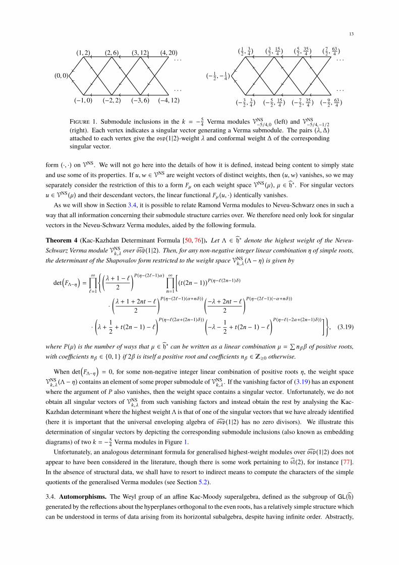
Figure 1. Submodule inclusions in the k = − 54 Verma modules VNS

−5/4,0 (left) and VNS−5/4,−1/2

(right). Each vertex indicates a singular vector generating a Verma submodule. The pairs (λ,∆)attached to each vertex give the osp(1|2)-weight λ and conformal weight ∆ of the correspondingsingular vector.

form (·, ·) on VNS. We will not go here into the details of how it is defined, instead being content to simply stateand use some of its properties. If u,w ∈ VNS are weight vectors of distinct weights, then (u,w ) vanishes, so we mayseparately consider the restriction of this to a form Fµ on each weight space VNS (µ ), µ ∈ h∗. For singular vectorsu ∈ VNS (µ ) and their descendant vectors, the linear functional Fµ (u, ·) identically vanishes.

As we will show in Section 3.4, it is possible to relate Ramond Verma modules to Neveu-Schwarz ones in such away that all information concerning their submodule structure carries over. We therefore need only look for singularvectors in the Neveu-Schwarz Verma modules, aided by the following formula.

Theorem 4 (Kac-Kazhdan Determinant Formula [50, 76]). Let Λ ∈ h∗ denote the highest weight of the Neveu-Schwarz Verma module VNS

k,λ over osp(1|2). Then, for any non-negative integer linear combination η of simple roots,the determinant of the Shapovalov form restricted to the weight space VNS

k,λ (Λ − η) is given by

det(FΛ−η

)=

∞∏`=1

(λ + 1 − `

2

)P (η−(2`−1)α ) ∞∏n=1

[(t (2n − 1))P (η−`(2n−1)δ )

·

(λ + 1 + 2nt − `

2

)P (η−(2`−1) (α+nδ )) (−λ + 2nt − `

2

)P (η−(2`−1) (−α+nδ ))

·

(λ +

12+ t (2n − 1) − `

)P (η−`(2α+(2n−1)δ )) (−λ −

12+ t (2n − 1) − `

)P (η−`(−2α+(2n−1)δ ))] , (3.19)

where P (µ ) is the number of ways that µ ∈ h∗ can be written as a linear combination µ =∑nβ β of positive roots,

with coefficients nβ ∈ 0, 1 if 2β is itself a positive root and coefficients nβ ∈ ≥0 otherwise.

When det(FΛ−η

)= 0, for some non-negative integer linear combination of positive roots η, the weight space

VNSk,λ (Λ − η) contains an element of some proper submodule of VNS

k,λ . If the vanishing factor of (3.19) has an exponentwhere the argument of P also vanishes, then the weight space contains a singular vector. Unfortunately, we do notobtain all singular vectors of VNS

k,λ from such vanishing factors and instead obtain the rest by analysing the Kac-Kazhdan determinant where the highest weight Λ is that of one of the singular vectors that we have already identified(here it is important that the universal enveloping algebra of osp(1|2) has no zero divisors). We illustrate thisdetermination of singular vectors by depicting the corresponding submodule inclusions (also known as embeddingdiagrams) of two k = − 5

4 Verma modules in Figure 1.Unfortunately, an analogous determinant formula for generalised highest-weight modules over osp(1|2) does not

appear to have been considered in the literature, though there is some work pertaining to sl (2), for instance [77].In the absence of structural data, we shall have to resort to indirect means to compute the characters of the simplequotients of the generalised Verma modules (see Section 5.2).

3.4. Automorphisms. The Weyl group of an affine Kac-Moody superalgebra, defined as the subgroup of GL (h)generated by the reflections about the hyperplanes orthogonal to the even roots, has a relatively simple structure whichcan be understood in terms of data arising from its horizontal subalgebra, despite having infinite order. Abstractly,

14 J SNADDEN, D RIDOUT, AND S WOOD

if W is the Weyl group of the horizontal subalgebra g, then the Weyl group W of the full affine superalgebra gdecomposes as

W W n Q∨0 , (3.20)

where Q∨0 is the coroot lattice of the even subalgebra g(0): the -span of the coroots α∨j for any choice of simpleroots α j of g(0) . The semidirect product structure is defined by the standard linear action of W on this lattice, as asubset of h.

In the case of osp(1|2), the (lone) simple coroot of the even subalgebra is (2α )∨, giving Q∨0 , with the Weylgroup W 2 acting by inversion on this lattice. The Weyl group W of osp(1|2) is thus isomorphic to the non-trivialsemidirect product of 2 with : the infinite dihedral group.

For both the Neveu-Schwarz and Ramond algebras, we define the conjugation automorphism w by

wen = −fn ,

wxn = −yn ,

whn = −hn ,

wK = K ,

wL0 = L0,

wfn = −en ,

wyn = xn ,(3.21a)

where we note that the restriction to the horizontal subalgebra gives precisely the conjugation automorphism w ofosp(1|2), as defined in Section 2.3. Similarly, the spectral flow automorphism σ is defined by

σ en = en−2,

σxn = xn−1,

σhn = hn − 2δn,0K ,

σK = K ,

σL0 = L0 − h0 + K ,

σ fn = fn+2,

σyn = yn+1.(3.21b)

When we need to distinguish the algebra on which the automorphism is acting, we shall furnish it with a subscript,as in wNS or wR. In addition, we define isomorphisms τ : gNS → gR and τ ′ : gR → gNS between the Neveu-Schwarzand Ramond algebras, both of which act on the basis elements according to

en 7−→ en−1,

xn 7−→ xn−1/2,

hn 7−→ hn − δn,0K ,

K 7−→ K ,

L0 7−→ L0 −12h0 +

14K ,

fn 7−→ fn+1,

yn 7−→ yn+1/2(3.21c)

(the indices n are constrained to range over the appropriate domains for gNS and gR). It is not hard to see thatτ ′ τ = σNS and τ τ ′ = σR. As such, we will from here on denote both τ and τ ′ by σ 1/2, using a subscript todistinguish (where necessary) which algebra is being acted upon.

Note that the automorphisms w and σ both preserve the Cartan subalgebra h and that their restrictions to h generatethe Weyl group W ⊆ GL (h). However, the automorphisms themselves satisfy w2 = (wσ )2 = 1 and therefore generatea group isomorphic to 4 n . As with osp(1|2), we cannot realise the Weyl group W as a subgroup of the innerautomorphisms of osp(1|2).

Nevertheless, just as we did in Section 2.3, we may promote both w and σ to functors on the module category ofeither the Neveu-Schwarz or Ramond algebra. In fact, since σ is of infinite order, we get a functor σn for each n ∈ .We shall refer to the images of a module M under w and σn as the conjugate and spectral flow of M, respectively.As in Section 2.3, it is clear that these functors commute with parity reversal. They moreover satisfy

wwM M, σmσnM σm+nM and wσnM σ−nwM, (3.22)

for allm,n ∈ , so we have indeed constructed a strict W-action on the set of osp(1|2)-module isomorphism classes.As in Section 2.3, this action can be lifted to the category of weight osp(1|2)-modules. We may also carry this outfor the isomorphisms σ 1/2, constructing functors between the two categories. These satisfy

σ 1/2σ 1/2M σM, (3.23)

so in fact we have spectral flow functors σn for each n ∈ 12. The isomorphisms of (3.22) also hold form,n ∈ 1

2.

15

Because the functors w and σn , n ∈ 12, are obviously invertible, they define equivalences between the corre-

sponding module categories. As a consequence, they preserve structure (submodules, quotients, Loewy diagrams,and so on). These functors turn out to be incredibly useful in analysing the representation theory of osp(1|2) andits associated vertex operator superalgebras. As an example, we remark that the claim made in Section 3.3 — thatthe structures of the Ramond Verma modules may be deduced from those of the Neveu-Schwarz Verma modules —now follows immediately from the identifications

VRk,λ wσ−1/2VNS

k,k−λ . (3.24)

Proving (3.24) is straightforward but illustrative. First, VNSk,k−λ is generated by a highest-weight vector v of osp(1|2)-

weight (k − λ)α , so wσ−1/2VNSk,k−λ is generated by wσ−1/2 (v ) (by the invertibility of the functors). Second, the

osp(1|2)-weight of wσ−1/2 (v ) is λα :

h0wσ−1/2 (v ) = wσ−1/2 (σ 1/2w(h0)v ) = wσ−1/2((−h0 + K )v

)= λwσ−1/2 (v ). (3.25)

Third, wσ−1/2 (v ) is a highest-weight vector (in the Ramond sector):

e0wσ−1/2 (v ) = wσ−1/2 (σ 1/2w(e0)v ) = wσ−1/2 (−f1v ) = 0,

y1/2wσ−1/2 (v ) = wσ−1/2 (σ 1/2w(y1/2)v ) = wσ−1/2 (x0v ) = 0.(3.26)

Finally, VNSk,k−λ is freely generated as a U (g−NS)-module so wσ−1/2VNS

k,k−λ is freely generated as a U (g−R)-module(wσ−1/2 maps g−NS onto g−R). This completes the proof.

It is important to note that the conjugation and spectral flow automorphisms of Section 3.4 obviously extend toautomorphisms of the universal enveloping algebra of osp(1|2) and thereby define automorphisms of the (universal)vertex superalgebra obtained from osp(1|2)k by forgetting the conformal structure. Twisting by conjugation orspectral flow therefore preserves the property of being a module of this vertex superalgebra.5 In fact, these twistsalso preserve the property of being a module of the vertex operator superalgebra. The only difference is that thespectral flow images of certain modules may now be distinguished from the original modules because spectral flowdoes not preserve the conformal structure (3.10), hence the conformal weights will change in general. In particular,this is the case for the vacuum module which is the vertex operator superalgebra regarded as a module over itself.

Finally, note that because automorphisms necessarily preserve the maximal proper ideal of osp(1|2)k , regardedas a vertex superalgebra, the arguments of the previous paragraph also apply to the minimal model vertex operatorsuperalgebras B0 |1 (u,v ). In particular, the category of B0 |1 (u,v )-modules is closed under twisting by conjugationand spectral flow.

Proposition 5.

(i) If M is an osp(1|2)k module, then its twists by spectral flow and conjugation, σnM and wM respectively, arealso osp(1|2)k modules.

(ii) If M is an B0 |1 (u,v ) module, then its twists by spectral flow and conjugation, σnM and wM respectively, arealso B0 |1 (u,v ) modules.

4. The affine minimal model B0 |1 (2, 4): Modules

Proposition 5 is noteworthy because the spectral flows of a given positive-energy module M will not (usually)be positive-energy for almost all n. It follows that the appropriate category of B0 |1 (u,v )-modules for constructing aconsistent conformal field theory is not likely to be a subcategory of the category of positive-energy weight modules.Consequently, much of the representation theory of these vertex operator superalgebras cannot be detected directlyby Zhu’s algebra. Nevertheless, it appears [24,25,27,35] that combining positive-energy classifications with spectralflow does lead to module categories that satisfy key consistency requirements, modular invariance for example.

5 We remark that our working definition of module of a vertex superalgebra follows that given by Frenkel and Ben-Zvi [78, Ch. 5.1], adding therequirement to be 2-graded by parity (as in Section 2.2). In particular, a module over the level-k universal vertex superalgebra associated toosp(1 |2) is just a smooth 2-graded level-k osp(1 |2)-module.

16 J SNADDEN, D RIDOUT, AND S WOOD

We shall therefore proceed with the classification of simple positive-energy B0 |1 (u,v )-modules using Zhu tech-nology, specialising to k = − 5

4 (u = 2, v = 4). The central charge of this minimal model is c = −5. We beginby reviewing the theory of (twisted) Zhu algebras, emphasising their realisations in terms of zero modes of vertexoperator superalgebra elements.

4.1. Zhu’s algebra. The associative algebras now known as Zhu algebras [79] form an invaluable formalism forclassifying positive-energy modules over vertex operator superalgebras. Essentially, the Zhu algebra of a vertexoperator superalgebra is the associative unital algebra of zero modes (of all fields) restricted to only act on groundstates, these being vectors that are annihilated by all positive field modes (we will make this precise below). Therelaxed highest-weight vectors of Section 3.2 are salient examples of ground states. Zhu’s formalism then guaranteesthat any moduleM over Zhu’s algebra can be induced to a vertex operator superalgebra moduleM, containingM inits space of ground states. Further, if M is simple, then the space of ground states of the unique simple quotient ofM is precisely M. So simple positive-energy modules are classified by first classifying simple modules over Zhu’salgebra and then taking the simple quotients of their inductions.

The Zhu algebra Zhu[V] for untwisted modules over a vertex operator superalgebra V was first studied in [80],while the Zhu algebra Zhuτ [V] for modules twisted by a finite order automorphism τ was introduced in [81]. In thecase at hand, the untwisted modules form the Neveu-Schwarz sector and the Ramond sector corresponds to modulestwisted by the parity automorphism. We refer to [65, App. A] for an introduction to Zhu’s algebras for general vertexoperator superalgebras, in both the twisted and untwisted cases. This introduction emphasises the fact that Zhu’salgebra is nothing but an abstraction of the algebra of zero modes acting on ground states.

With this fact in mind, the most straightforward way to define the untwisted Zhu algebra for affine vertex operatorsuperalgebras is as follows. Let Uk (osp(1|2)) denote the quotient of U(osp(1|2)) by the ideal generated byK −k1 andlet Uk (osp(1|2))0 be its conformal weight zero subalgebra (the centraliser of L0 in Uk (osp(1|2))). Then, there is aprojection π0 : Uk (osp(1|2))0 → U(osp(1|2)) whose kernel is spanned by the Poincaré-Birkhoff-Witt basis elements,ordered by increasing mode index, that involve modes with non-zero indices (we identify zero modes with elementsof osp(1|2)). The untwisted Zhu algebra Zhu

[osp(1|2)k

]is then the image of the map

v ∈ osp(1|2)k 7−→ [v] = π0 (v0), (4.1)

where v0 is the zero mode of the field6 corresponding to v (and π0 has been extended to an appropriate completionof Uk (osp(1|2))0). Zhu’s associative product ∗ is then given by

[u] ∗ [v] = π0 (u0v0). (4.2)

The equivalence of this definition with Zhu’s original one, in the case of affine vertex operator superalgebras,follows from noting that π0 merely implements the constraint that the zero modes act on ground states. We referto [65, App. A] for further information.

The twisted Zhu algebra Zhuτ[osp(1|2)k

]and its associative product are defined in almost precisely the same

manner using the same formulae. We shall distinguish the twisted image of an element v from its untwisted cousin[v] by a superscript: [v]τ ∈ Zhuτ

[osp(1|2)k

]. The main difference is that we must restrict the defining map to the

bosonic orbifold of osp(1|2)k (the subalgebra of even elements) because the odd elements have no zero mode whenacting in the Ramond sector.

The following proposition was proved in [82] for affine Kac-Moody algebras and in [80] for the untwisted Zhualgebras of affine Kac-Moody superalgebras. We are not aware of a source that proves the twisted Zhu algebra resultin the latter case though it is surely very well known.

Proposition 6. The untwisted and twisted Zhu algebras of osp(1|2)k are

Zhu[osp(1|2)k

]= U(osp(1|2)), Zhuτ

[osp(1|2)k

]= U(sl (2)). (4.3)

6For v of definite conformal weight ∆v , we assume a mode expansion for the corresponding field of the form v (z ) =∑n vnz−n−∆v .

17

Proof. By construction, Zhu[osp(1|2)k

]lies in U(osp(1|2)). However, it is easy to check that any monomial

j1 · · · jn ∈ U(osp(1|2)) can be realised, up to a sign coming from parities, as the image in Zhu[osp(1|2)k

]of an

element of osp(1|2)k , namely jn−1 · · · j

1−1Ωk (here, Ωk denotes the vacuum vector of osp(1|2)k ). This demonstrates

equality as vector spaces. To show equality as associative algebras, we only need show that the Zhu elementsj ≡ j0 = π0 (j0) = [j−1Ωk ], j = h, e, f ,x ,y, satisfy the same commutation rules with respect to ∗ as they do inU(osp(1|2)). This is, of course, exactly how ∗ is defined:

j1 ∗ j2 − (−1) |j1 | |j2 | j2 ∗ j1 = π0 (j

10 j

20 ) − (−1) |j

1 | |j2 |π0 (j20 j

10 ) = π0 ([j10, j

20]) = π0 ([j1, j2]0) = [j1, j2]. (4.4)

We recall that |j | ∈ 0, 1 denotes the parity of j.The argument identifying Zhuτ

[osp(1|2)k

]is practically identical once one has shown that it lies in U(sl (2)). All

that we can conclude at present is that Zhuτ[osp(1|2)k

]lies in the even subalgebra of U(osp(1|2)) (which strictly

contains U(sl (2))). To show that it indeed lies in U(sl (2)), consider an even element u ∈ osp(1|2)k . Choosing aPoincaré-Birkhoff-Witt ordering in which odd modes appear to the right of even modes (and are then ordered byincreasing index), u is expressed as a linear combination of monomials · · · j1

−m−1j2−n−1Ωk , where either the modes

appearing are all even or both j1−m−1 and j2

−n−1 are odd withm,n ∈ ≥0.Consider the image of each such monomial in the twisted Zhu algebra. If j1

−m−1 and j2−n−1 are both odd, then we

apply the following identity (obtained by applying π0 to [65, Eq. (A.2)] with k =m + 1, n =m − 12 ):

[· · · j1−m−1j

2−n−1Ωk

]τ= −

∞∑`=0

(1/2` + 1

) [· · · j1

−m+` j2−n−1Ωk

]τ, m ∈ ≥0. (4.5)

Inductively, the index r of j1 can then be made non-negative at which point we note that

j1r j2−n−1Ωk = j1r , j2−n−1Ωk , r ≥ 0, (4.6)

replaces the two odd modes by an even one (and perhaps a constant). We conclude that a monomial with a pair of oddmodes is equivalent, in Zhuτ

[osp(1|2)k

], to a linear combination ofmonomials inwhich these oddmodes are replaced

by an even mode. By performing this replacement for all odd modes, it follows as before that Zhuτ[osp(1|2)k

]lies

in U(sl (2)). The rest of the argument is identical to the untwisted case.

For a given admissible level k, recall that χk denotes the singular vector that generates the (unique) maximalproper ideal of osp(1|2)k by which one quotients in order to obtain the minimal model vertex operator superalgebraB0 |1 (u,v ). By the Kac-Kazhdan formula of Theorem 4, one can determine that the conformal weight and osp(1|2)-weight of χk are 1

2 (u − 1)v and (u − 1)α , respectively. Define ϕk = yu−10 χk and note that this descendant of χk has

osp(1|2)-weight 0.

Proposition 7. The untwisted and twisted Zhu algebras of B0 |1 (u,v ) are

Zhu[B0 |1 (u,v )

]

U(osp(1|2))⟨[ϕk

]⟩ , Zhuτ[B0 |1 (u,v )

]

U(sl (2))⟨[ϕk

]τ ⟩ , (4.7)

where⟨[ϕk

]⟩and

⟨[ϕk

]τ ⟩ are the two-sided ideals generated by the images of ϕk in Zhu[osp(1|2)k

] U(osp(1|2))

and Zhuτ[osp(1|2)k

] U(sl (2)), respectively.

Proof. Note that while ϕk is a zero mode descendant of χk , the converse is also true: χk is a zero mode descendantof ϕk . This follows either by explicitly evaluating xu−1

0 ϕk or by noting that finite-dimensional osp(1|2) modules aresemisimple and that the space of vectors in osp(1|2)k of conformal weight 1

2 (u − 1)v is finite-dimensional. Thus,every vector in the maximal proper ideal of osp(1|2)k is a descendant of ϕk by non-positive modes.

We have to show that the image of the maximal proper ideal in Zhu’s algebra is generated by the image of ϕk .To this end, let j and v be homogeneous vectors in osp(1|2)k and suppose that j has conformal weight 1. In theNeveu-Schwarz sector, the corresponding fields j (z) and v (z) will have zero modes, regardless of their parities, and

18 J SNADDEN, D RIDOUT, AND S WOOD

we have the following identities in Zhu[osp(1|2)k

]:

[j0v] = [j] ∗ [v] − (−1) |j | |v |[v] ∗ [j], [j−m−1v] = (−1)m (−1) |j | |v |[v] ∗ [j], m ≥ 0. (4.8)

The first follows from [j0,v0] = (j0v )0, while the second follows from (j−m−1v ) (z) =1m! :∂m j (w )v (w ): . It follows

inductively that if the image of v in Zhu[osp(1|2)k

]belongs to the image of the maximal proper ideal, then so do

the images of all the descendants of v by non-positive modes. Taking v = ϕk establishes the untwisted result.In the Ramond sector, j (z) and v (z) will only have zero modes if they have even parity. In this case, the identities

(4.8) also hold in Zhuτ[osp(1|2)k

]if we replace [·] by [·]τ . As above, we conclude that the images of all the

descendants of ϕk by non-positive evenmodes belong to the ideal generated by [ϕk ]τ in Zhuτ[osp(1|2)k

]. However,

as in the proof of Proposition 6, even non-positive mode descendants of ϕk have images that are equivalent to a linearcombination of non-positive mode descendants in which all odd modes are zero modes. Since the action of the zeromodes on ϕk generates a simple weight osp(1|2)-module whose even subspace is a simple weight sl (2)-module, byTheorem 2, each pair of odd zero modes may be replaced by an even zero mode. We conclude that the image ofevery even non-positive mode descendant of ϕk is in the ideal of U(sl (2)) generated by [ϕk ]τ , as required.

Remark. We mention that in the proof of Proposition 6, we could remove the odd zero modes along with the positivemodes because they annihilate Ωk . In the proof of Proposition 7 above, ϕk need not be annihilated by the odd zeromodes, hence they are not removed.

Remark. This proposition remains true for Zhu[B0 |1 (u,v )

]if we replace ϕk by χk throughout. The proof follows

along the same lines with minor adjustments. For Zhuτ[B0 |1 (u,v )

], we can make this replacement if χk is even.

The simple positive-energy Neveu-Schwarz modules of B0 |1 (u,v ) are the simple quotients of the inductions ofthe simple Zhu

[B0 |1 (u,v )

]-modules, while the simple positive-energy Ramond modules of B0 |1 (u,v ) are the simple

quotients of the inductions of the simple Zhuτ[B0 |1 (u,v )

]-modules. Moreover, the simple Zhu

[B0 |1 (u,v )

]-modules

are precisely those of Theorem 2 on which[ϕk

]acts trivially, while the simple Zhuτ

[B0 |1 (u,v )

]-modules are those

of Theorem 1 on which[ϕk

]τ acts trivially.The level of interest here is k = − 5

4 , thus u = 2 and v = 4 in the setup of (3.15), which implies that the singularvector has conformal weight 2 and osp(1|2)-weight α . One choice of normalisation of this vector is

χ−5/4 = (x−2 − 4y−1e−1 + 2h−1x−1)Ω−5/4. (4.9)

Then,ϕ−5/4 = y0χ−5/4 =

(h−2 + 2h2

−1 + 8f−1e−1 + 6y−1x−1)Ω−5/4. (4.10)

Proposition 8. The images of ϕ−5/4 in the untwisted and twisted Zhu algebras are

[ϕ−5/4] = Σ(2Σ − 1), [ϕ−5/4]τ = 4Q +158, (4.11)

where Σ and Q are the super-Casimir of osp(1|2) and the Casimir of sl (2), respectively.

Proof. The proof is very similar to proofs in [62–65], so we will only briefly outline the reasoning. Since theosp(1|2)-weight of ϕ−5/4 is 0, its images in the Zhu algebras will also have weight 0 and hence these images lie in thecentralisers of the Cartan subalgebras C(h,U(osp(1|2))) and C(h,U(sl (2))). Further, since these images are uniquelydetermined by their action on weight spaces, all that remains to complete this proof is the computation of this action.

The field corresponding to ϕ−5/4 is

ϕ (z) = ∂h(z) + 2 :h(z)h(z): + 8 :f (z)e (z): + 6 :y (z)x (z): (4.12)

and thus its zero mode isϕ0 = −h0 + 2 :hh: 0 + 8 :f e: 0 + 6 :yx : 0. (4.13)

Evaluating ϕ0 on a Neveu-Schwarz ground state vector uλ,s of osp(1|2)-weight λα and Σ-eigenvalue s produces

ϕ0uλ,s =(−h0 + 2h2

0 + 8e0 f0 − 6x0y0)uλ,s = s (2s − 1)uλ,s , (4.14)

19

where the normally ordered products were evaluated using (3.13a). Thus, the image of ϕ−5/4 in Zhu[osp(1|2)k

]is

Σ(2Σ − 1), as required.Similarly, evaluating ϕ0 on a Ramond ground state vλ,q of sl (2)-weight λα and Q-eigenvalue q produces

ϕ0vλ,q =

(−h0 + 2h2

0 + 8e0 f0 + 6(

516−

12h0

))vλ,q =

(4q +

158

)vλ,q , (4.15)

where the odd normally ordered product :yx : 0 was evaluated using (3.13b). This, in turn, implies that the image ofϕ−5/4 in Zhuτ

[osp(1|2)k

]is 4Q + 15

8 , completing the proof.

4.2. Classifying B0 |1 (2, 4)-modules. Given our explicit identifications of the untwisted and twisted Zhu algebrasZhu

[B0 |1 (2, 4)

]and Zhuτ

[B0 |1 (2, 4)

], we can now easily classify the simple relaxed highest-weight B0 |1 (2, 4)-

modules in both the Neveu-Schwarz and Ramond sectors.

Theorem 9. Any simple Neveu-Schwarz relaxed highest-weight B0 |1 (2, 4)-module is isomorphic to one of thefollowing mutually non-isomorphic modules:

A0, B+−1/2, B−1/2,

ΠA0, ΠB+−1/2, ΠB−1/2,

CΛ,0 (Λ ∈ /2 \ [± 12 ]). (4.16)

We remark that the parity reversal of CΛ,0 is isomorphic to CΛ+1,0, by (2.14), so does appear in the list above.

Proof. The space of ground states of any simple Neveu-Schwarz relaxed highest-weight B0 |1 (2, 4)-module must beisomorphic to one of the simple osp(1|2)-modules listed in Theorem 2 on which [ϕ−5/4] = Σ(2Σ − 1) acts trivially.The given classification consists of precisely those simple quotients of the inductions of the osp(1|2)-modules forwhich this is the case.

Remark. One potential source of confusion that is worth mentioning is that as 12 is an allowed eigenvalue of the

super-Casimir Σ, yet − 12 is not, any simple Zhu

[B0 |1 (2, 4)

]-module with a weight space on which the eigenvalue of

Σ is 12 cannot have any weight spaces of opposite parity. The only simple osp(1|2)-modules satisfying this constraint

are A0 and its parity reversal.

Remark. The gaps in the range of Λ, for CΛ,0, in the previous theorem are only to guarantee simplicity. Thereducible, but indecomposable, modules C±1/2+2,0 and C±

−1/2+2,0 have ground states that obviously satisfy the Zhuconstraints, hence they are also B0 |1 (2, 4)-modules (in the Neveu-Schwarz sector).

Given that all the C-type B0 |1 (2, 4)-modules have s = 0, we shall simplify notation in what follows by writing Cλ ,C±1/2 and C±

−1/2 instead of Cλ+2,0, C±1/2+2,0 and C±−1/2+2,0, respectively. We shall also further abuse this notation

by identifying λ with Λ = λ + 2 when convenient, so that λ ∈ /2 when parametrising a C-type module.

Theorem 10. Any simple Ramond relaxed highest-weight B0 |1 (2, 4)-module is isomorphic to one of the followingmutually non-isomorphic modules:

D+−5/4, D+

−3/4, D−3/4, D−5/4 EΛ,−15/32,

ΠD+−5/4, ΠD+

−3/4, ΠD−3/4, ΠD−5/4 ΠEΛ,−15/32(Λ ∈ /2 \ [± 5

4 ]). (4.17)

Proof. The space of ground states of any simple Ramond relaxed highest-weight B0 |1 (2, 4)-module must be isomor-phic to one of the simple sl (2)-modules listed in Theorem 1 on which [ϕ−5/4]τ = 4Q + 15

8 acts trivially. The givenclassification consists of those simple quotients of the inductions of the sl (2)-modules for which this is the case.

Remark. Again, the gaps in the range of Λ, for EΛ,−15/32, in the previous theorem guarantee simplicity. Thereducible, but indecomposable, modules E±λ+2,−15/32, with λ = ±

54 , are also B0 |1 (2, 4)-modules (in the Ramond

sector).

Because all these E-type modules have q = − 1532 , we shall again simplify notation in what follows by writing Eλ

instead of Eλ+2,−15/32, for λ , 54 mod 2, and E±λ instead of E±λ+2,−15/32, for λ = ±

54 . As above, we shall also abuse

this notation by identifying λ with Λ = λ + 2 when parametrising E-type modules.

20 J SNADDEN, D RIDOUT, AND S WOOD

These theorems classify the simple positive-energy weight modules over B0 |1 (2, 4) because a weight vector ofminimal conformal weight in a simple module must generate the entire module and hence must be a relaxed highest-weight vector. However, we can also twist each of these modules by conjugation and/or spectral flow (Proposition 5).If we twist by conjugation, the result will again be a simple positive-energy weight module. Explicitly, we have

wA0 A0, wB+−1/2 B−1/2, wCλ C−λ (λ , ± 1

2 mod 2),

wD+−5/4 D−5/4, wD+

−3/4 D−3/4, wEλ E−λ (λ , ± 54 mod 2).

(4.18)

The conjugates of the spectral flows of these modules now follow (formally) from (3.22).However, twisting these simple positive-energy weight modules by spectral flow will not result in modules that are

positive-energy, in general. Naïvely, we arrive at the following list of (isomorphism classes of) simple Neveu-Schwarzweight modules (we also include their parity reversals, recalling that ΠCλ Cλ+1):

σ `A0, σ `B+−1/2, σ `B−1/2, σ `Cλ (` ∈ and λ , 1

2 mod 1),

σ `D+−3/4, σ `D+

−5/4, σ `D−3/4, σ `D−5/4, σ `Eµ (` ∈ + 12 and µ , ± 5

4 mod 2).(4.19)

The simple Ramond weight modules are obtained from these by applying σ 1/2 to each of the above. It turns outhowever, that these lists contain many pairs of isomorphic modules. In particular, it is easy to show (using similartechniques to those used in the proof of (3.24)) that the following coincidences hold:

σ 1/2A0 D+−5/4, σ−1/2A0 D−5/4,

σ 1/2B−1/2 D+−3/4, σ−1/2B+

−1/2 D−3/4.(4.20)

With these isomorphisms in mind, the list of (isomorphism classes of) mutually non-isomorphic simple weightmodules over B0 |1 (2, 4) reduces to

σ `A0, σ `B+−1/2, σ `B−1/2, σ `Cλ , σ `Eµ (4.21)

and their parity reversals, where ` ∈ 12, λ ,

12 mod 1 and µ , ± 5

4 mod 2. To establish that these isomorphismclasses are indeed distinct, one may observe that their spaces of extremal states are different, these being the weightvectors of minimal conformal weight in each subspace of constant osp(1|2)-weight.

We shall assume that the physical category P relevant for constructing minimal model conformal field theorieshas precisely the modules (4.21) as its simple objects. We shall also assume that the category is closed underconjugation and fusion products. One of the main aims of this paper is to test this assumption by demonstratingthat it leads to satisfactory modular properties and that the standard Verlinde formula, introduced below in (7.6b),returns non-negative integer Grothendieck fusion coefficients.

The assumption of closure under fusion is highly non-trivial from amathematical perspective because the modulesin P, in particular the relaxed highest-weight modules Cλ , Eµ and their spectral flows, are not all C1-cofinite. Thismeans that fusion products might not be finite-length (meaning that they have a finite number of composition factors).However, the failure of C1-cofiniteness is also observed with relaxed modules for admissible-level sl (2) minimalmodels and bosonic ghosts [35], whilst the known fusion calculations [19,26,35] all give finite-length results. Thesecalculations were performed using the Nahm-Gaberdiel-Kausch algorithm [83,84] whose (essential) equivalence tothe rigorous theory of Huang, Lepowsky and Zhang [85] will appear in [86]. The results give us confidence that ourassumptions on the B0 |1 (2, 4) fusion rules all hold, though they will be extremely difficult to establish rigorously.

The conjugates and spectral flow images of the reducible but indecomposable B0 |1 (2, 4)-modules identified aboveare, likewise, reducible but indecomposable weight modules over B0 |1 (2, 4), by Proposition 5. The conjugates areeasily identified using (3.22):

wC+1/2 C−−1/2, wE+3/4 E−

−3/4, wE+5/4 E−−5/4. (4.22)

Up to parity reversal, we therefore obtain the following mutually non-isomorphic reducible, but indecomposable,modules:

σ `C+1/2, σ `C−−1/2, σ `E+3/4, σ `E+5/4, σ `E−

−3/4, σ `E−−5/4 (` ∈

12). (4.23)

21

We record the defining non-split short exact sequences, easily deduced from (3.18), for future convenience:

0 −→ ΠB+−1/2 −→ C+1/2 −→ B−1/2 −→ 0,

0 −→ D+−5/4 −→ E+3/4 −→ D−3/4 −→ 0,

0 −→ D+−3/4 −→ E+5/4 −→ D−5/4 −→ 0,

0 −→ ΠB−1/2 −→ C−−1/2 −→ B+

−1/2 −→ 0,

0 −→ D−5/4 −→ E−−3/4 −→ D+

−3/4 −→ 0,

0 −→ D−3/4 −→ E−−5/4 −→ D+

−5/4 −→ 0.

(4.24)

Sequences for the spectral flows of these modules now follow because the σ ` induce exact covariant functors.These results indicate that the minimal model B0 |1 (2, 4) provides another example of a conformal field theory

to which the standard module formalism of [27, 28] applies. To wit, the simple modules σ `Cλ and σ `Eµ comprisethe typical modules, while the reducible modules of (4.23) are examples of atypical modules. Together, the C- andE-type modules, along with their spectral flows, constitute the standard modules of the minimal model. Subquotientsof atypical modules are also said to be atypical, hence the σ `A0 and σ `B∓

±1/2 are all atypical and thus so are theσ `D∓

±3/4 and σ`D∓±5/4.

The standard module formalism is a collection of empirical observations, first described in [29], that coherentlyorganises the modular properties of a large number of logarithmic conformal field theories. To summarise, thecharacters of the standard modules (which form a continuously parametrised family) transform rather simply undera natural action of SL(2;) with integral kernels replacing the familiar S- and T-matrices. The transforms ofthe atypical characters, which include that of the vacuum module, are much more subtle, but may be deduced byconstructing infinite (one-sided) resolutions of each atypical module in terms of standard ones. This rich formalismwill provide the starting point for our investigation of the modular properties of the minimal model. First however,we need to determine the characters of these modules.

5. The affine minimal model B0 |1 (2, 4): Characters

In this section, we determine the characters and supercharacters of all the simple B0 |1 (2, 4)-modules of categoryP. We also introduce the Grothendieck group of this category and show explicitly that the images of the standardB0 |1 (2, 4)-modules in the Grothendieck group form a basis (of a certain completion).

5.1. Highest-weight characters. Having identified themodules of interest, we nowwish to calculate their characters.Formally, the character of a weight-module M of osp(1|2) is defined to be the power series

ch0[M

] (y, z,q

)= tr

M

(ykzh0qL0−c/24

), (5.1)

where trM(X ) denotes the trace of the image in End(M) of X ∈ h under the given representation of osp(1|2). We

append the subscript 0 to our notation for characters to indicate that eigenvectors of different parities count equallyin the sum. The notation for supercharacters, where parity matters, will be introduced in Section 5.3. It is customaryto interpret such an expression as defining a (meromorphic) function, however some care is needed to make thisidentification precise. In particular, we must additionally specify a domain for the variables z and q in order to avoidmisleading results (further discussion of this may be found in [22, 24]).

It is clear thatch0

[ΠM

]= ch0

[M

], (5.2)

for any weight module M over osp(1|2), so it might appear that we are justified in identifying modules with theirparity reversals, at least for the purposes of studying modular transformations. However, we shall see that the parityof a module is completely determined by its character and supercharacter, so one can employ modular methods whilstretaining parity information.

As discussed in Section 3.3, the characters of the simple highest-weight B0 |1 (2, 4)-modules can be expressed interms of Verma module characters using resolutions. As usual, the characters of Verma modules are very easy tocalculate. A straightforward application of the Poincaré-Birkhoff-Witt theorem gives, recalling that c = −5,

ch0[VNS

0

] (y, z,q

)= y−5/4q5/24

∞∏m=1

(1 + z−1qm−1

)(1 + zqm )(

1 − z−2qm−1) (1 − qm )(1 − z2qm

) , (5.3)

22 J SNADDEN, D RIDOUT, AND S WOOD

which can be re-expressed more compactly as

ch0[VNS

0

] (y, z,q

)= −iy−5/4z1/2q1/4 ϑ2 (z;q)

ϑ1 (z2;q) η(q), (5.4)

using the standard infinite product formulae for the Jacobi theta functions ϑj and the Dedekind eta function η. Moregenerally, a simple calculation shows that Neveu-Schwarz Verma characters are given by

ch0[VNSλ

] (y, z,q

)= zλq∆ch0

[VNS

0

] (y, z,q

), (5.5)

where ∆ was given in (3.14). This relation holds for all non-critical k, simply by replacing the exponent of y by k.From the embeddings of Verma modules shown in Figure 1, it follows that the characters of the simple Neveu-

Schwarz highest-weight B0 |1 (2, 4)-modules are given by

ch0[A0

] (y, z,q

)=

∑n∈2

ch0[VNS−5/4,n

] (y, z,q

)−

∑n∈2+1

ch0[VNS−5/4,n

] (y, z,q

)=

∑n∈

(−1)nznqn (n+1)ch0[VNS

0

] (y, z,q

)= y−5/4ϑ1 (z;q2) ϑ2 (z;q)

ϑ1 (z2;q) η(q), (5.6a)

ch0[B+−1/2

] (y, z,q

)=

∑n∈2

ch0[VNSn−1/2

] (y, z,q

)−

∑n∈2+1

ch0[VNSn−1/2

] (y, z,q

)=

∑n∈

(−1)nzn−1/2qn2−1/4ch0

[VNS

0

] (y, z,q

)= −iy−5/4ϑ4 (z;q2) ϑ2 (z;q)

ϑ1 (z2;q) η(q). (5.6b)

In order to calculate the characters of B−1/2 wB+−1/2 and the other twists of these highest-weight modules, we

use the following relation:trφ (M) (X ) = tr

M

(φ−1 (X )

)(φ ∈ Aut (g), X ∈ h). (5.7)

Specialising to φ = w and σ ` , ` ∈ 12, we obtain the useful formulae

ch0[wM

] (y, z,q

)= ch0

[M

] (y, z−1,q

), ch0

[σ `M

] (y, z,q

)= ch0

[M

] (yz2`q`

2, zq`,q

), (5.8)

the latter following from σ `h0 = h0 − 2`K and σ `L0 = L0 − `h0 + `2K . Under the transformation z 7→ z−1, the

Jacobi theta functions ϑj (z;q), for j = 2, 3, 4, are invariant whilst ϑ1 (z−1;q) = −ϑ1 (z;q). We therefore arrive at the

character of B−1/2 wB+−1/2:

ch0[B−1/2

] (y, z,q

)= ch0

[B+−1/2

] (y, z−1,q

)= iy−5/4ϑ4 (z;q2) ϑ2 (z;q)

ϑ1 (z2;q) η(q). (5.9)

Whilst it is tempting to treat the expressions in (5.6a), (5.6b) and (5.9) as defining meromorphic functions of(y, z,q), doing so means that we must carefully restrict their domains. Outside of the appropriate domain of validity,these meromorphic functions will give different power series expansions about the origin. Since characters aredefined precisely by such expansions, a given meromorphic function may correspond to a multitude of differentcharacters.

It turns out that (5.6a) is valid (and its right-hand side is convergent), for all y, z,q ∈ with y , 0, 0 < |q | < 1and z restricted to the annulus

|q |1/2 < |z | < |q |−1/2. (5.10)

In particular, this includes z = 1, which one should expect, given that the L0-eigenspaces of A0 are all finite-dimensional. Similarly, (5.6b) and (5.9) are valid for y , 0, 0 < |q | < 1 and z restricted to the disjoint annuli

1 < |z | < |q |−1/2 and |q |1/2 < |z | < 1, (5.11)

respectively. Note that neither of the modules B±∓1/2 has finite-dimensional L0-eigenspaces, so their characters must

indeed diverge at z = 1.

23

In order to calculate the characters of the spectral flows of the above modules, we apply (5.8). For example, usingthe properties of Jacobi theta functions, we obtain

ch0[σ `A0

] (y, z,q

)= (−1)`/2y−5/4ϑ1 (z;q2) ϑ2 (z;q)

ϑ1 (z2;q) η(q), (5.12a)

if ` is even, and

ch0[σ `A0

] (y, z,q

)= i(−1) (`−1)/2y−5/4ϑ4 (z;q2) ϑ2 (z;q)

ϑ1 (z2;q) η(q), (5.12b)

if ` is odd. It may seem, at first glance, that this sequence of characters holds a (perhaps surprising) four-foldperiodicity. This semblance breaks down however, once we take into account the domains on which these expressionsare valid. Specifically, (5.12a) and (5.12b) will only recover the appropriate characters, as formal power series, whenexpanded in the domain 0 < |q | < 1 and

|q |1/2−` < |z | < |q |−1/2−`, (5.13)

as follows from Equations (5.8) and (5.10).We can now apply (4.20) and (5.8) to the character formulae (5.6) and (5.9) in order to calculate the characters of

the Ramond highest-weight modules and their conjugates. We summarise the results, along with the Neveu-Schwarzformulae presented above, in the following proposition.

Proposition 11. The characters of the highest-weight B0 |1 (2, 4)-modules are given by the following expressions,valid for y , 0, 0 < |q | < 1 and z in the annuli given:

ch0[A0

] (y, z,q

)= y−5/4ϑ1 (z;q2) ϑ2 (z;q)

ϑ1 (z2;q) η(q)(|q |1/2 < |z | < |q |−1/2),

ch0[B+−1/2

] (y, z,q

)= −iy−5/4ϑ4 (z;q2) ϑ2 (z;q)

ϑ1 (z2;q) η(q)(1 < |z | < |q |−1/2),

ch0[D+−5/4

] (y, z,q

)= −iy−5/4z−1/4q1/16ϑ4 (zq

−1/2;q2) ϑ3 (z;q)ϑ1 (z2;q) η(q)

(1 < |z | < |q |−1),

ch0[D+−3/4

] (y, z,q

)= y−5/4z−1/4q1/16ϑ1 (zq

−1/2;q2) ϑ3 (z;q)ϑ1 (z2;q) η(q)

(1 < |z | < |q |−1/2).

(5.14)

Remark. The characters of the conjugates of the highest-weight B0 |1 (2, 4)-modules are now easily computed usingEquation (5.8), noting that A0 is self-conjugate:

ch0[B−1/2

] (y, z,q

)= iy−5/4ϑ4 (z;q2) ϑ2 (z;q)

ϑ1 (z2;q) η(q)(|q |1/2 < |z | < 1),

ch0[D−5/4

] (y, z,q

)= −y−5/4z−1/4q1/16ϑ1 (zq

−1/2;q2) ϑ3 (z;q)ϑ1 (z2;q) η(q)

(|q | < |z | < 1),

ch0[D−3/4

] (y, z,q

)= iy−5/4z−1/4q1/16ϑ4 (zq

−1/2;q2) ϑ3 (z;q)ϑ1 (z2;q) η(q)

(|q |1/2 < |z | < 1).

(5.15)

The characters of the remaining simple atypical B0 |1 (2, 4)-modules are similarly obtained using spectral flow.

5.2. Relaxed highest-weight characters. For osp(1|2), there seems to be no literature addressing the submodulestructure of relaxed Verma modules. Even though character formulae for relaxed Verma modules over osp(1|2) areeasy to obtain, we are therefore unable to deduce character formulae for their simple quotients. Instead, we resort toan indirect method developed for sl (2)-modules in [24, 25] and rigorously justified in [73].

We start with the short exact sequences given in (4.24) for the reducible, but indecomposable, Neveu-Schwarzrelaxed highest-weight modules C±

±1/2, immediately deducing the following character formulae:

ch0[C±±1/2

]= ch0

[B+−1/2

]+ ch0

[B−1/2

]. (5.16)

Of course, this only holds when treating these characters as formal power series. Since the two expressions (5.6b)and (5.9) that we have derived for the characters on the right-hand side, are valid on disjoint domains, we must

24 J SNADDEN, D RIDOUT, AND S WOOD

be careful to sum these characters as power series rather than as meromorphic functions — naïvely summing thederived characters, as meromorphic functions, gives zero! For this, we appeal to the following (equivalent) identities,originally derived by Kac and Wakimoto in [87]:

ϑ1 (uv;q) η(q)3

ϑ1 (u;q) ϑ1 (v;q)= −i

∑m∈

um

1 −vqm(|q | < |u | < 1, 0 < |v | < |q | < 1), (5.17a)

ϑ1 (uv;q) η(q)3

ϑ1 (u;q) ϑ1 (v;q)= −i

∑m∈

umvqm

1 −vqm(1 < |u | < |q |−1, 0 < |v | < |q | < 1). (5.17b)

We refer to [22, App. B] for the conventions on θ functions used here. Setting u = z2 and rearranging, these become

1ϑ1 (z2;q)

= −iϑ1 (v;q)

ϑ1 (z2v;q) η(q)3∑m∈

z2m

1 −vqm(|q |1/2 < |z | < 1, 0 < |v | < |q | < 1), (5.18a)

1ϑ1 (z2;q)

= −iϑ1 (v;q)

ϑ1 (z2v;q) η(q)3∑m∈

z2mvqm

1 −vqm(1 < |z | < |q |−1/2, 0 < |v | < |q | < 1). (5.18b)

We substitute (5.18a) into the character formula (5.9), noting that both have the same domain of validity, obtaining

ch0[B−1/2

] (y, z,q

)= y−5/4ϑ4 (z;q2) ϑ2 (z,q)

η(q)4ϑ1 (v;q)ϑ1 (z2v;q)

∑m∈

z2m

1 −vqm. (5.19)

Performing the equivalent substitution of (5.18b) into (5.6b) (which also have the same domain of validity), weinstead get

ch0[B+−1/2

] (y, z,q

)= −y−5/4ϑ4 (z;q2) ϑ2 (z,q)

η(q)4ϑ1 (v;q)ϑ1 (z2v;q)

∑m∈

z2mvqm

1 −vqm. (5.20)

Treating these as formal power series in z, we may forget their domains and sum them, giving

ch0[C±±1/2

] (y, z,q

)= y−5/4ϑ4 (z;q2) ϑ2 (z,q)

η(q)4ϑ1 (v;q)ϑ1 (z2v;q)

∑m∈

z2m . (5.21)

In this way, we have arrived at a character formula for the reducible Neveu-Schwarz relaxed highest-weight modules.These are precisely the atypical standard modules in the Neveu-Schwarz sector.

We may simplify the character formula (5.21) further and eliminate the auxiliary variable v, but we must firstintroduce an alternative set of variables for the characters. Instead of giving characters as power series in y, z,q, it isstandard (and essential for studying modular properties) to introduceψ , ζ and τ , defined by

y = e2π iψ , z = e2π iζ and q = e2π iτ . (5.22)

The relation between z and ζ will be used repeatedly in the following manipulations.Identifying the sum on the right-hand side of (5.21) as defining a distribution in ζ , we can employ the Fourier-

theoretic identity ∑n∈

e2π inw =∑n∈

δ (w − n) (5.23)

to make the following simplification:

ϑ1 (v;q)ϑ1 (z2v;q)

∑m∈

z2m =ϑ1 (v;q)

ϑ1 (e4π iζv;q)

∑m∈

δ (2ζ −m) =∑m∈

ϑ1 (v;q)ϑ1 (e2π imv;q)

δ (2ζ −m) =∑m∈

e−π imδ (2ζ −m). (5.24)

Here, we have noted that ϑ1 (e2π iv;q) = eπ iϑ1 (v;q). Now,

ch0[C±±1/2

] (y, z,q

)= y−5/4ϑ4 (z;q2) ϑ2 (z;q)

η(q)4

∑m∈

e−π imδ (2ζ −m)

= y−5/4 1η(q)4

∑m∈

ϑ4 (eπ im ;q2) ϑ2 (eπ im ;q)eπ im

δ (2ζ −m), (5.25)

25

which can be split into sums over even and odd values ofm, giving

ch0[C±±1/2

] (y, z,q

)= y−5/4 1

η(q)4

∑n∈

(−1)n[ϑ4 (1;q2) ϑ2 (1;q) δ (2ζ − 2n)

+ ϑ3 (1;q2) ϑ1 (1;q) δ (2ζ − 2n − 1)]. (5.26)

However, ϑ1 (1;q) vanishes identically, so that

ch0[C±±1/2

] (y, z,q

)= y−5/4ϑ4 (1;q2) ϑ2 (1;q)

2η(q)4∑n∈

eπ inδ (ζ − n) = y−5/4ϑ4 (1;q2) ϑ2 (1;q)2η(q)4

∑n∈

zn+1/2. (5.27)

The q-dependent factor can be further simplified, using the product forms of the Jacobi theta functions, giving ourfinal result:

ch0[C±±1/2

] (y, z,q

)=y−5/4z1/2

η(q)2

√ϑ2 (1;q)2η(q)

∑n∈

zn . (5.28)

We remark that the decoupling of the z- and q-dependences of this character is expected for a module whose groundstates form a dense osp(1|2)-module.

It is convenient, at this point, to extract the q-dependent terms from (5.28) in the following definition:

Aj (q) =1

η(q)2

√ϑj (1;q)η(q)

(j = 2, 3, 4). (5.29)

We can rewrite these factors explicitly as

A2 (q) =√

2q−1/24∞∏i=1

1 + qi

(1 − qi )2, A3 (q) = q

−5/48∞∏i=1

1 + qi−1/2

(1 − qi )2, A4 (q) = q

−5/48∞∏i=1

1 − qi−1/2

(1 − qi )2. (5.30)

Inserting into (5.28) and expanding, one finds that

ch0[C±±1/2

] (y, z,q

)= y−5/4z1/2A2 (q)

√2

∑n∈

zn = y−5/4z1/2q−1/24∞∏i=1

1 + qi

(1 − qi )2·∑n∈

zn

= y−5/4z1/2q−1/24(1 + 3q + 8q2 + 19q3 + 41q4 + 83q5 + · · ·

) ∑n∈

zn (5.31)

which indeed gives the correct weight multiplicities (shown for the first six conformal grades) of C±±1/2. We mention

that the prefactor q−1/24 = q∆−c/24, requires that ∆ = − 14 (recall that c = −5), in accord with s = 0 and (3.17).

A similar calculation gives the characters of the atypical relaxed Ramond modules. We record these results in thefollowing proposition.

Proposition 12. The characters of the atypical relaxed B0 |1 (2, 4)-modules are (shifted) formal power series in z

whose coefficients are holomorphic functions of q for |q | < 1. Explicitly, we have

ch0[C±±1/2

] (y, z,q

)=y−5/4z1/2√

2A2 (q)

∑n∈

zn , (5.32a)

ch0[E±±5/4

] (y, z,q

)= ch0

[E∓∓3/4

] (y, z,q

)=y−5/4z±5/4

2*,A3 (q)

∑n∈

zn +A4 (q)∑n∈

(−z)n+-. (5.32b)

With (5.8), we can now compute the characters of all the atypical standard modules. However, we also need tocompute the characters of the typical standard modules: the Cλ , the Eµ and their spectral flows. Happily, these maybe deduced from those of the atypical standards merely by shifting the powers of z in (5.28) and (5.32b).

Proposition 13. The characters of the typical relaxed B0 |1 (2, 4)-modules are (shifted) formal power series in z

whose coefficients are holomorphic functions of q for |q | < 1. Explicitly, we have

ch0[Cλ

] (y, z,q

)=y−5/4zλ√

2A2 (q)

∑n∈

zn (λ , ±12

mod 2), (5.33a)

26 J SNADDEN, D RIDOUT, AND S WOOD

ch0[Eµ

] (y, z,q

)=y−5/4zµ

2*,A3 (q)

∑n∈

zn +A4 (q)∑n∈

(−z)n+-

(µ , ±54

mod 2). (5.33b)

We will not provide a proof of this assertion here, referring instead to recent work of Adamović [88, Sec. 11] whoproves (5.33a) using an explicit construction of these modules. A more general proof, that includes the Ramondcase (5.33b), appears in [73]. This approach works in the setting of affine Lie superalgebras and relies on Mathieu’stheory of coherent families [89]. We expect it to also generalise to higher rank superalgebras.

Remark. Wenote that the Ramond characters (5.33b) aremanifestly 2-periodic in µ, in accordwith the isomorphismsEµ Eµ+2. However, the Neveu-Schwarz characters (5.33a) are manifestly 1-periodic, despite Cλ and Cλ+1 beingnon-isomorphic. Rather, we have Cλ ΠCλ+1, by (2.14), explaining this 1-periodicity.

5.3. Supercharacters. As mentioned above, modular transformations require us to consider supercharacters inaddition to characters. The supercharacter of a weight module M of osp(1|2) is defined, analogously to thedefinition of character in (5.1), to be the formal power series

ch1/2[M

] (y, z,q

)= str

M

(ykzh0qL0−c/24

)(5.34)

in which strM(X ) denotes the supertrace of the image in End(M) of X ∈ h. This is, we recall, the trace of X on the

even subspaceM(0) minus the trace on the odd subspaceM(1) . The use of the subscript 12 turns out to be convenient

in Section 6, see Equation (6.6) for example. We clearly have

ch1/2[ΠM

]= −ch1/2

[M

](5.35)

and, similarly to characters, supercharacters of twisted modules are easily computed using

ch1/2[wM

] (y, z,q

)= ch1/2

[M

] (y, z−1,q

), ch1/2

[σ `M

] (y, z,q

)= ch1/2

[M

] (yz2`q`

2, zq`,q

), (5.36)

the latter holding for all ` ∈ 12.

In fact, it is easy to deduce formulae for osp(1|2)-module supercharacters from their character formulae because xand y have odd osp(1|2)-weights (measured in units of α) while e, h and f have even osp(1|2)-weights. The vectorsof an osp(1|2)-module M whose osp(1|2)-weights are even, relative to some chosen (even) vector, therefore spanM(0) while those with relative odd osp(1|2)-weights span M(1) . Replacing z by eiπz = −z everywhere in ch0

[M

],

except in the prefactor that fixes the osp(1|2)-weight of the chosen vector, will therefore convert the character of Minto its supercharacter. The supercharacters of the relaxed highest-weight B0 |1 (2, 4)-modules are thereby deducedfrom Propositions 11 to 13.

Proposition 14. The supercharacters of the simple B0 |1 (2, 4)-modules are specified, for |q | < 1, by

ch1/2[A0

] (y, z,q

)= y−5/4ϑ2 (z;q2) ϑ1 (z;q)

ϑ1 (z2;q) η(q)(|q |1/2 < |z | < |q |−1/2),

ch1/2[B+−1/2

] (y, z,q

)= −iy−5/4ϑ3 (z;q2) ϑ1 (z;q)

ϑ1 (z2;q) η(q)(1 < |z | < |q |−1/2),

ch1/2[Cλ

] (y, z,q

)=y−5/4zλ√

2A2 (q)

∑n∈

(−z)n (λ , ±12

mod 2),

ch1/2[Eµ

] (y, z,q

)=y−5/4zµ

2*,A4 (q)

∑n∈

zn +A3 (q)∑n∈

(−z)n+-

(µ , ±54

mod 2)

(5.37)

and (5.36) (conjugation and spectral flow). Similarly, the supercharacters of the atypical standardB0 |1 (2, 4)-modulesare specified by

ch1/2[C±±1/2

] (y, z,q

)=y−5/4z1/2√

2A2 (q)

∑n∈

(−z)n ,

ch1/2[E±±5/4

] (y, z,q

)= ch1/2

[E∓∓3/4

] (y, z,q

)=y−5/4z±5/4

2*,A4 (q)

∑n∈

zn +A3 (q)∑n∈

(−z)n+-.

(5.38)

27

Remark. Note that ch1/2[Cλ

]is 1-antiperiodic in λ and ch1/2

[Eµ

]is 2-periodic in µ, as expected.

5.4. The Grothendieck group. Given a category C of modules, each of which has finitely many compositionfactors, one defines its Grothendieck group [C] as the free abelian group generated by the isomorphism classes ofthe simple modules. The image [M] ∈ [C] of a module M ∈ C is then the sum of the images of its compositionfactors. As characters and supercharacters are isomorphism invariants that do not distinguish between a module andthe direct sum of its composition factors, they define functions ch0 and ch1/2 on the Grothendieck group.

Neither of these functions is injective — in general, ch0 and ch1/2 do not distinguish [M] from [ΠM] and −[ΠM],respectively — but their direct sum is, provided that the set of pairs (ch0[M], ch1/2[M]), where [M] ranges over theisomorphism classes of the simple modules, is linearly independent (over ). If this is the case, which it is for thephysical category P of B0 |1 (2, 4)-modules, then it follows that the character and supercharacter of a module togethercompletely determine the class of the module in the Grothendieck group.

Whilst the set of isomorphism classes of the simple B0 |1 (2, 4)-modules should be regarded as a canonical basisof the Grothendieck group, the standard module formalism suggests that another basis set will be useful. This is theset of Grothendieck images of the standard modules, both typical and atypical, noting that

[σ `C+1/2

]=

[Πσ `B+

−1/2

]+

[σ `B−1/2

]=

[Πσ `C−

−1/2

](5.39a)

in the Neveu-Schwarz sector, whilst in the Ramond sector we similarly have[σ `E+3/4

]=

[σ `E−

−5/4

],

[σ `E+5/4

]=

[σ `E−

−3/4

](5.39b)

and their parity-reversed counterparts. To maintain linear independence among the images of the atypical standards,we may consistently omit the Grothendieck images of standards with − superscripts in favour of those with +superscripts. There is, of course, no issue with linear independence among typicals.

We assert that the Grothendieck images of the typicals and the atypical standards with + superscripts togetherform a basis of a certain completion of the Grothendieck group of our B0 |1 (2, 4)-module category P. To justify this,we must exhibit the images of the simple atypicals as a linear combination of images of atypical standards. This isachieved by constructing resolutions for the former in terms of the latter. It clearly suffices to give the resolutions forone member of each spectral flow orbit of simple atypicals.

Proposition 15. The simple modules A0 and B∓±1/2 have the following resolutions:

· · · −→ Πσ 11/2E+3/4 −→ σ 5C+1/2 −→ σ 9/2E+5/4

−→ σ 7/2E+3/4 −→ Πσ 3C+1/2 −→ Πσ 5/2E+5/4

−→ Πσ 3/2E+3/4 −→ σC+1/2 −→ σ 1/2E+5/4 −→ A0 −→ 0, (5.40a)

· · · −→ Πσ 11/2E+5/4 −→ Πσ 9/2E+3/4 −→ σ 4C+1/2

−→ σ 7/2E+5/4 −→ σ 5/2E+3/4 −→ Πσ 2C+1/2

−→ Πσ 3/2E+5/4 −→ Πσ 1/2E+3/4 −→ C+1/2 −→ B−1/2 −→ 0, (5.40b)

· · · −→ σ 6C+1/2 −→ σ 11/2E+5/4 −→ σ 9/2E+3/4

−→ Πσ 4C+1/2 −→ Πσ 7/2E+5/4 −→ Πσ 5/2E+3/4

−→ σ 2C+1/2 −→ σ 3/2E+5/4 −→ σ 1/2E+3/4 −→ B+−1/2 −→ 0. (5.40c)

Proof. The resolutions are constructed by repeatedly splicing the following short exact sequences, their parityreversals and their spectrally flowed versions:

0 −→ σB−1/2 −→ σ 1/2E+5/4 −→ A0 −→ 0,

0 −→ ΠB+−1/2 −→ C+1/2 −→ B−1/2 −→ 0,

0 −→ σA0 −→ σ 1/2E+3/4 −→ B+−1/2 −→ 0.

(5.41)

These, in turn, are easily derived from the short exact sequences (4.24) and the identifications (4.20).

28 J SNADDEN, D RIDOUT, AND S WOOD

The Euler-Poincaré principle now leads to the desired expressions for the images of the simple atypicals in anappropriate completion of the Grothendieck group. Such a completion must admit the required infinite sums and sowe shall choose it to consist of (possibly infinite) linear combinations of the form

n∑i=1

∑`≥L

aiL[σ `Si

](n ∈ ≥0, L ∈ 1

2, aiL ∈ ), (5.42)

where each Si is either a typical or an atypical standard with + superscript. The key requirement is that the spectralflow indices be bounded below. The Grothendieck images of the typicals and atypical standards with + superscriptsform a basis of this completion, in the obvious sense, as claimed.

Remark. The above completion allows for the following interpretation. Let((σ 1/2

))be the ring of formal Laurent

series in the spectral flow functor σ 1/2. 7 These series can then be applied to finite sums of (Grothendieck imagesof) standards to get infinite sums of the form (5.42). In other words, the set of all elements of the form (5.42) is justthe free

((σ 1/2

))-module whose basis consists of all typicals and all atypical standards with + superscript.

Corollary 16. The following identities hold in the given completion of the Grothendieck group (as do their spectrallyflowed versions):

[A0

]=

∞∑n=0

( [σ 4n+1/2E+5/4

]−

[σ 4n+1C+1/2

]+

[Πσ 4n+3/2E+3/4

]

−[Πσ 4n+5/2E+5/4

]+

[Πσ 4n+3C+1/2

]−

[σ 4n+7/2E+3/4

]), (5.43a)

[B−1/2

]=

∞∑n=0

( [σ 4nC+1/2

]−

[Πσ 4n+1/2E+3/4

]+

[Πσ 4n+3/2E+5/4

]

−[Πσ 4n+2C+1/2

]+

[σ 4n+5/2E+3/4

]−

[σ 4n+7/2E+5/4

]), (5.43b)

[B+−1/2

]=

∞∑n=0

( [σ 4n+1/2E+3/4

]−

[σ 4n+3/2E+5/4

]+

[σ 4n+2C+1/2

]

−[Πσ 4n+5/2E+3/4

]+

[Πσ 4n+7/2E+5/4

]−

[Πσ 4n+4C+1/2

]). (5.43c)

Applying ch0 and ch1/2 to these identities then gives analogous identities for simple atypical (super)characters interms of atypical standard (super)characters.

It is easy to check that the infinite sums of (super)characters in these relations converge in the sense of formal powerseries. This means that the coefficient of each monomial in the indeterminates only receives non-zero contributionsfrom finitely many of the terms in the infinite sum.

Remark. Note that one can also derive right-sided resolutions for the simple atypicals, for example by takingcontragredient duals of the left-sided ones of Proposition 15. The powers of spectral flow appearing in theseresolutions and the analogue of Corollary 16 would then be bounded above.

The natural completion of the Grothendieck group would now be the free ((σ−1/2

))-module on the typicals and

atypical standards with + superscript. One can check that the results derived in what follows do not depend on thechoice of resolutions.

6. The affine minimal model B0 |1 (2, 4): Modular properties

We now study the modular properties of the simple and standard B0 |1 (2, 4)-modules. More precisely, we firstshow that the action of the modular group closes on the span of the characters and supercharacters of the standardmodules. From Section 5.4, the characters and supercharacters of the simple atypical B0 |1 (2, 4)-modules belong to

7Recall that in rings of formal Laurent series, the powers of the indeterminate are assumed to be bounded below.

29

this span, so their modular properties follow directly. These explicit modular transformations will be used to computethe Grothendieck fusion rules in Section 7 using a version of the standard Verlinde formula.

6.1. Standard modular transforms. The modular group SL(2;) admits the following well known presentation:

SL(2;) =⟨S, T : S2 = (ST)3, S4 = 1

⟩. (6.1)

On (super)characters, we define the action of the generating elements S and T to be the coordinate transforms

S(ψ |ζ |τ ) =(ψ −

ζ 2

τ+

12πk

(argτ −

π

2

) ζ

τ

−1τ

), T(ψ |ζ |τ ) =

(ψ +

112k

ζ

τ + 1

), (6.2)

where k = − 54 (and we recall Equation (5.22) for the definition ofψ , ζ and τ ). Though the transform forψ may appear

unfamiliar, it is chosen specifically to obtain an honest, as opposed to a projective, representation of SL(2;) onthe span of the standard characters. Direct computation verifies that these generators do indeed satisfy the definingrelations (6.1) of SL(2;).

The modular transformations of the standard characters can be computed from those of the auxiliary functionsA2 (q), A3 (q) and A4 (q) defined in (5.29):

SA2 (q)

=

1−iτ

A4 (q), SA3 (q)

=

1−iτ

A3 (q), SA4 (q)

=

1−iτ

A2 (q),

TA2 (q)

= e−π i/12A2 (q), T

A3 (q)

= e−5π i/24A4 (q), T

A4 (q)

= e−5π i/24A3 (q).

(6.3)

These formulae follow directly from the well known transforms of the Jacobi theta functions and the Dedekind etafunction.

In preparation for the modular S-transforms below, we rewrite the formulae for the standard (super)charactersusing the Fourier theoretic identity (5.23). For example,

ch0[Cλ

]= ykzλ

A2 (q)√

2

∑n∈

zn = ykA2 (q)√

2

∑n∈

zλδ (ζ − n) = ykA2 (q)√

2

∑n∈

e2π iλnδ (ζ − n) (6.4)

implies, using (5.8), that

ch0[σ `Cλ

]= (yz2`q`

2)kA2 (q)√

2

∑n∈

e2π iλnδ (ζ + `τ − n)

= ykA2 (q)√

2

∑n∈

e2π iλne2π ik`(2n−`τ )δ (ζ + `τ − n). (6.5a)

Similarly,

ch1/2[σ `Cλ

]= yk

A2 (q)√

2

∑n∈

e2π iλ (n−1/2)e2π ik`(2n−1−`τ )δ (ζ + `τ + 12 − n), (6.5b)

ch0[σ `Eµ

]= yk *

,

A3 (q)

2

∑n∈

e2π iµne2π ik`(2n−`τ )δ (ζ + `τ − n)

+A4 (q)

2

∑n∈

e2π iµ (n−1/2)e2π ik`(2n−1−`τ )δ (ζ + `τ + 12 − n)

+-, (6.5c)

ch1/2[σ `Eµ

]= yk *

,

A4 (q)

2

∑n∈

e2π iµne2π ik`(2n−`τ )δ (ζ + `τ − n)

+A3 (q)

2

∑n∈

e2π iµ (n−1/2)e2π ik`(2n−1−`τ )δ (ζ + `τ + 12 − n)

+-. (6.5d)

These formulae also cover the (super)characters of the atypical standard modules. Note that we can write theseformulae in the succinct forms

chε[σ `Cλ

]= yk

A2 (q)√

2

∑n∈+ε

e2π iλne2π ik`(2n−`τ )δ (ζ + `τ − n), (6.6a)

30 J SNADDEN, D RIDOUT, AND S WOOD

chε[σ `Eλ

]= yk*.

,

A3 (q)

2

∑n∈+ε

+A4 (q)

2

∑n∈+1/2+ε

+/-

e2π iλne2π ik`(2n−`τ )δ (ζ + `τ − n), (6.6b)

where ε ∈ 0, 12. It will be useful in what follows to think of ε as living in the two element abelian group where

addition is taken mod 1.

Proposition 17. For ` ∈ 12, and λ ∈ , let

KT` (λ) = e2π i`(k`+λ) . (6.7)

Then, the T-transforms of the standard (super)characters are given by the following formulae:

Tchε

[σ `Cλ

]= eπ i/12KT

` (λ) chε+`[σ `Cλ

], (6.8a)

Tchε

[σ `Eλ

]= e−π i/24KT

` (λ) chε+`+1/2[σ `Eλ

]. (6.8b)

Proof. The proof follows by substituting the appropriate transformation formula from (6.3) into the (super)characterformulae (5.33). For example, the C-type (super)characters give

Tchε

[σ `Cλ

]= eπ i/6yke−π i/12A2 (q)

√2

∑n∈+ε

e2π iλne2π ik`(2n−`τ−`)δ (ζ + `τ + ` − n)

= eπ i/12ykA2 (q)√

2

∑n∈+ε+`

e2π iλ (n+`)e2π ik`(2n−`τ+`)δ (ζ + `τ − n)

= eπ i/12KT` (λ) chε+`

[σ `Cλ

]. (6.9)

The E-type case proceeds in the same way.

We conclude that T acts diagonally on Neveu-Schwarz (super)characters, whilst in the Ramond sector, it takesa character to (a multiple of) the supercharacter of the same module and vice versa. The behaviour of the (su-per)characters under the S-transform is similar, though the explicit formulae are slightly more complicated.

Proposition 18. For `, `′ ∈ 12 and λ, λ′ ∈ , let

KS`,`′ (λ, λ

′) = e−2π i(2k``′+`′λ+`λ′) . (6.10)

Then, the S-transforms of the standard (super)characters are given by the following formulae:

Schε

[σ `Cλ

]=

1√

2

∑`′∈+ε

∫/2

KS`,`′ (λ, λ

′) ch`+1/2[σ `′Eλ′

]dλ′, (6.11a)

Schε

[σ `Eλ

]=

1√

2

∑`′∈+ε+1/2

∫/

KS`,`′ (λ, λ

′) ch`[σ `′Cλ′

]dλ′

+12

∑`′∈+ε

∫/2

KS`,`′ (λ, λ

′) ch`[σ `′Eλ′

]dλ′. (6.11b)

Proof. As a preparatory step, we record the S-transform of the common prefactoryk of the (super)character formulae:

Syk

= e2π ik (ψ−ζ 2/τ )ei(arg τ−π /2) =

−iτ

|τ |yke2π ik (−ζ 2/τ ) . (6.12)

The S-transforms of the proposition now follow by evaluating the left- and right-hand sides and comparing. Forexample,

Schε

[σ `Cλ

]=−iτ

|τ |yke2π ik (−ζ 2/τ ) 1

−iτ

A4 (q)√

2

∑n∈+ε

e2π iλne2π ik`(2n+`/τ )δ (ζ − `

τ− n)

= ykA4 (q)√

2

∑n∈+ε

e2π in (λ−knτ )δ (ζ − ` − nτ ), (6.13)

31

where we have used the identity |a |δ (az) = δ (z), while1√

2

∑`′∈+ε

∫/2

e−2π i(2k``′+`′λ+`λ′)ch`+1/2[σ `′Eλ′

]dλ′

=1√

2

∑`′∈+ε

e−2π i`′ (2k`+λ)yk∫/2

*.,

A3 (q)

2

∑n∈+`+1/2

e2π iλ′ (n−`)e2π ik`′ (2n−`′τ )δ (ζ + `′τ − n)

+A4 (q)

2

∑n∈+`

e2π iλ′ (n−`)e2π ik`′ (2n−`′τ )δ (ζ + `′τ − n)+-

dλ′

= ykA4 (q)√

2

∑`′∈+ε

e−2π i`′ (λ+k`′τ )δ (ζ − ` + `′τ ), (6.14)

where we have used the identity∫/2 e2π iλ′mdλ′ = 2δm,0 form ∈ 1

2. Setting `′ = −n completes this case. The

Ramond case is similar.

By a slight abuse of nomenclature, we shall from here on refer to the integration kernels appearing in the integrals(6.11) as S-matrix coefficients. The coefficient of the (super)character of a moduleM′ appearing in the S-transformof the (super)character of a moduleM will be denoted by Sε,ε ′[M→M′], where ε and ε ′ take values 0 or 1

2 to referto the character or supercharacter of M and M′, respectively. With this convention, we may rewrite (6.11) in theform

Sε,ε ′[σ `Cλ → σ `′Cλ′

]= 0, Sε,ε ′

[σ `Eλ → σ `′Cλ′

]=

1√

2KS`,`′ (λ, λ

′)1`=ε ′1`′,ε ,

Sε,ε ′[σ `Cλ → σ `′Eλ′

]=

1√

2KS`,`′ (λ, λ

′)1`,ε ′1`′=ε , Sε,ε ′[σ `Eλ → σ `′Eλ′

]=

12KS`,`′ (λ, λ

′)1`=ε ′1`′=ε ,

(6.15)

where the condition in the index of the characteristic function 1• (which is 1 when • is true and 0 otherwise) isalways understood to be taken mod 1 whenever it involves an ε.

This notation allows us to define the transpose of the S-matrix elements in the obvious way:

Sε,ε ′[M→M′

] t= Sε ′,ε

[M′ →M

]. (6.16)

The adjoint † is then defined to be the (complex) conjugate transpose, as usual. We now see that with respect to thestandard basis of characters and supercharacters,

chε

[σ `Cλ

], chε

[σ `Eµ

]: ε ∈ 0, 1

2, ` ∈ 12, λ ∈ /, µ ∈ /2

, (6.17)

the S-matrix entries of Equation (6.15) are manifestly symmetric with respect to transposition. One can also checkthat the S- and T-transforms are unitary in the sense that T†T = 1 = S†S. For example, the (C → C)-type entries ofS†S are (because Sε,ε ′′[σ `Cλ → σ `′′Cλ′′] = 0)∑

ε ′′

∑`′′∈ 1

2

∫/2

Sε,ε ′′[σ `Cλ → σ `′′Eλ′′

]∗Sε ′′,ε ′

[σ `′′Eλ′′ → σ `′Cλ′

]dλ′′

=12

∑ε ′′

∑`′′∈ 1

2

1`,ε ′′1`′′=ε1`′′=ε ′1`′,ε ′′e2π i(2k (`−`′)`′′+(λ−λ′)`′′∫/2

e2π i(`−`′)λ′′ dλ′′

= 1ε=ε ′1`=`′∑

`′′∈+ε

e2π i(λ−λ′)`′′ = δε,ε ′δ`,`′δ (λ = λ′ mod 1)e2π iε (λ−λ′) . (6.18)

The result matches the corresponding entries of the identity operator because we should take λ = λ′ (choosing afundamental domain for / in the basis (6.17)), so that e2π iε (λ−λ′) = 1. If we had insisted on taking λ′ = λ + 1instead, then we would have obtained an additional sign when ε = 1

2 . This sign is naturally explained by the fact thatthe Neveu-Schwarz supercharacters satisfy ch1/2[σ `Cλ+1] = ch1/2[Πσ `Cλ] = −ch1/2[σ `Cλ].

6.2. Atypical modular transforms. Given the modular S- and T-transforms of the standard modules, it is now easyto compute the corresponding transforms of a given atypical simple (super)character using Corollary 16. We could

32 J SNADDEN, D RIDOUT, AND S WOOD

instead compute these transforms using the formulae of Section 5.1 which, after all, are already expressed in termsof theta functions. However, these formulae only represent the correct character on an appropriate annulus in thez-plane, which becomes a horizontal strip in the ζ -plane. It is easy to see that the modular S-transform does notrespect these strips, so one must meromorphically continue the character in ζ in order to get good modular properties.Unfortunately, different strips correspond to different spectral flows of the atypical simple module. The upshot is, aswas first noted in [22], that meromorphically continuing the characters in ζ leads to a loss of linear independence.

The standard module formalism, expressing the atypical simple (super)characters as linear combinations ofstandard (super)characters, neatly sidesteps this linear independence problem by treating all (super)characters asformal power series in z whose coefficients are meromorphic functions of q (in the unit disc). We therefore combinethe results of Corollary 16 and Proposition 18 to deduce (extending the notation in an obvious way) the S-matrixentries involving atypicals.

Proposition 19. The S-matrix entries describing the decomposition of the S-transforms of the atypical simplemodules are

Sε,ε ′[σ `A0 → σ `′Cλ′

]=

KS`,`′

(0, λ′)

2√

2 cos(πλ′)1`,ε ′1`′,ε ,

Sε,ε ′[σ `A0 → σ `′Eλ′

]=

KS`,`′

(0, λ′)

4 cos(πλ′) + 2√

21`,ε ′1`′=ε ,

Sε,ε ′[σ `B±

∓1/2 → σ `′Cλ′]=

KS`,`′

(∓ 12 , λ

′)

2√

2 cos(πλ′)1`,ε ′1`′,ε ,

Sε,ε ′[σ `B±

∓1/2 → σ `′Eλ′]=

(1 +√

2e∓π iλ′) KS

`,`′(∓ 1

2 , λ′)

4 cos(πλ′) + 2√

21`,ε ′1`′=ε .

(6.19)

Proof. The calculations are all very similar, so we only detail one example:

Sε,ε ′[σ `A0 → σ `′Cλ′

]=

∞∑n=0

(Sε,ε ′

[σ `+4n+1/2E+5/4 → σ `′Cλ′

]+ (−1)2εSε,ε ′

[σ `+4n+3/2E+3/4 → σ `′Cλ′

]

−(−1)2εSε,ε ′[σ `+4n+5/2E+5/4 → σ `′Cλ′

]− Sε,ε ′

[σ `+4n+7/2E+3/4 → σ `′Cλ′

] )=

e−2π i(`+2) (2k`′+λ′)√

2

∞∑n=0

e−8π iλ′n · 2i((−1)2`

′

sin(3πλ′) + (−1)2ε sin(πλ′))1`,ε ′1`′,ε

=e−2π i`(2k`′+λ′)

√2

sin(3πλ′) − sin(πλ′)sin(4πλ′)

1`,ε ′1`′,ε

=e−2π i`(2k`′+λ′)

√2

12 cos(πλ′)

1`,ε ′1`′,ε . (6.20)

Note here that the denominator should be expanded in non-negative powers of e−π iλ′ .

7. The affine minimal model B0 |1 (2, 4): Grothendieck fusion rules

This final section applies the modular S-transforms, computed explicitly in the previous section, to the calculationof the Grothendieck fusion rules of B0 |1 (2, 4). This requires a version of the Verlinde formula and we begin bydeducing such a formula, valid for vertex operator superalgebras like the one under consideration, from the standardVerlinde formula of its bosonic orbifold. The latter is of course conjectural, but has (in this case) already passed onevery stringent consistency test: the coefficients computed by the standard Verlinde formula for the bosonic orbifoldof B0 |1 (2, 4) are all non-negative integers [25].

7.1. AVerlinde formula for B0 |1 (2, 4). The purpose of this section is to determine the standard Verlinde formula forthe B0 |1 (2, 4) Grothendieck fusion ring. This is a formula for the (super)characters of fusion products of B0 |1 (2, 4)-modules that uses only the modular properties of the (super)characters as input data. As knowing the character andsupercharacter of a module in the category P amounts to knowing the image of the module in the Grothendieck group,

33

this formula allows us to compute fusion at the level of the Grothendieck group, thereby turning the Grothendieckgroup into a ring. Of course, this ring structure will only be well defined if fusing with any module of P defines anexact endofunctor of P. We conjecture that this is indeed the case, though we have no proof. The results obtainedbelow serve, among many things, as a consistency check on this conjecture.

We arrive at the standard Verlinde formula by interpreting B0 |1 (2, 4) as a simple current extension of its bosonicorbifold — the vertex operator algebra formed by the even elements of B0 |1 (2, 4) — and then lifting the standardVerlinde formula of the orbifold back to B0 |1 (2, 4). In the case at hand, the bosonic orbifold is actually isomorphic tothe sl (2) minimal model vertex operator algebra A1 (3, 4) of level − 5

4 , see [25, Sec. 10], although this identification isnot needed for what follows. The aim of the standard Verlinde formula is to determine the Grothendieck fusion rulesof B0 |1 (2, 4) directly without recourse to those of the orbifold. Of course, it is easy, in this particular example, to usethe orbifold’s Grothendieck fusion rules (which were computed in [25]), but the point is to develop the methodologyin a generality that applies for all admissible levels.

In order to be concise, we shall in this subsection denote the affine minimal model B0 |1 (2, 4) by V. Its bosonicorbifold vertex operator algebra (isomorphic to A1 (3, 4)) will be denoted by O. Let × denote the fusion productof V-modules and let ×O denote the fusion product of O-modules. Denote by ↓ the restriction of V-modules toO-modules and by ↑ the induction of O-modules to V-modules. We note the following relevant properties andassumptions (which are understood to be in force):

(i) The vertex operator superalgebra V is a order 2 simple current extension of O, that is, there exists a simpleO-module J such that J ×O J O and V↓ O ⊕ J. This property is expected for all bosonic orbifolds and hasbeen proven rigorously under certain hypotheses in [90,91]. While these works do not address vertex operatorsuperalgebras per se, their methods are easily adapted to this situation (see [92, App. A]). Unfortunately, therequired hypotheses are not known to be satisfied in our case, but this property was verified in [25, see Prop. 15and Sec. 10] under the assumption that the standard Verlinde formula for O A1 (3, 4) computes Grothendieckfusion coefficients for O-modules.

(ii) V admits a set of even parity standard modules S = S0 ∪ S1/2, where S0 and S1/2 denote the sets ofeven parity standard modules in the Neveu-Schwarz and Ramond sectors, respectively. This means that thecharacters and supercharacters of the modules in S span a representation of the modular group and everysimple module admits a resolution in terms of these modules and their parity reversals. For ξ = 0, 1

2 , letS Oξ be the set of O-modules that are obtained as direct summands of restrictions of V-modules in Sξ . Then,

S O = S O0 ∪S O

1/2 forms a set of standard O-modules.(iii) The fusion products of V and O are compatible, that is, for any O-modules W and X,

W↑ × X↑ (W ×O X)↑. (7.1)

This was proven in [28] under the assumption that × and ×O associate. This assumption may be removed [93]if the O-modules form a vertex tensor category in the sense of Huang, Lepowsky and Zhang [85]. However,this is not known for the categories we consider; nevertheless, we assume that (7.1) holds.

(iv) Fusing with a V-module from the given category P of V-modules defines an exact endofunctor on P. Similarly,fusing with an O-module defines an exact endofunctor on the category obtained by applying the restrictionfunctor to P. In other words, the corresponding Grothendieck fusion products are well defined.

(v) The standard module formalism of [27, 28] applies to the orbifold vertex operator algebra O, so that

ch[W

]O ch

[X

]= ch

[W ×O X

]=

∫S O

[Y

W X

]

Och

[Y

]dY (7.2a)

for any (appropriate) O-modules W and X, where O denotes the Grothendieck fusion product of O,[

Y

W X

]

O=

∫S O

s[W→ Z

]s

[X→ Z

]s

[Y→ Z

]∗

s[O→ Z

] dZ (7.2b)

34 J SNADDEN, D RIDOUT, AND S WOOD

is a Grothendieck fusion coefficient forO, and s[· → ·

]denotes theS-matrix entries of theO-module characters

(in the basis of standard characters). This is the most important assumption that we are making. It was alsoassumed in [25] when deriving the Grothendieck fusion rules for all admissible level sl (2) minimal models.Equation (7.2b) is the standard Verlinde formula for O.

These assumptions imply the following easy consequences.

Corollary 20.

(i) The restriction of any V-moduleM decomposes as

M↓ M(0) ⊕M(1) M(0) ⊕ (J ×O M(0) ) (O ⊕ J) ×O M(0) V↓ ×O M(0), (7.3)

where M(0) and M(1) J ×O M(0) denote the O-submodules consisting of the even and odd elements of M,respectively.

(ii) The simple current J has no fixed points: ifW is a simple O-module, then J ×O W W.(iii) For any V-moduleM, the inductions of M(0) andM(1) are given by

M(0)↑ M, M(1)↑ ΠM. (7.4)

(iv) For any V-moduleM, we have

chε[M

]= ch

[M(0)

]+ (−1)2εch

[M(1)

]=

(ch

[O

]+ (−1)2εch

[J

] )O ch

[M(0)

]. (7.5)

We now state the standard Verlinde formula for V. For this, it is convenient to treat the parameter ξ ∈ 0, 12 that

distinguishes the Neveu-Schwarz and Ramond sectors (see assumption (ii) above) as an element of 2.

Theorem 21. Let M and N be V-modules and let ξ and ξ ′ be 0 or 12 , depending on whether M and N are in the

Neveu-Schwarz or Ramond sector, respectively. Under the assumptions (i)–(v) above, we then have

chε[M

] chε

[N

]= chε

[M × N

]=

∫Sξ +ξ ′

[P

M N

]

εchε

[P

]dP, (7.6a)

where the Verlinde coefficients of V, indexed by ε = 0 (characters) or ε = 12 (supercharacters), are given by the

following standard Verlinde formula:[

P

M N

]

ε=

∫Sε+1/2

Sε,ξ+1/2[M→ Q

]Sε,ξ ′+1/2

[N → Q

]Sε,ξ+ξ ′+1/2

[P→ Q

]∗

Sε,1/2[V→ Q

] dQ. (7.6b)

We refer to the[

PM N

]εas Verlinde coefficients, rather than Grothendieck fusion coefficients, because they depend

upon whether we compute the character (ε = 0) or supercharacter (ε = 12 ) of the fusion product. Of course, knowing

both allows one to deduce the true Grothendieck fusion coefficients (Section 5.4) which will be denoted by[

PM N

].

We shall prove Theorem 21 below after recording some additional identities as preparatory lemmas. First however,we note that (7.6b) may be simplified by noting that all the S-matrix elements (6.15) and (6.19) may be factored asfollows:

Sε,ε ′[M→ N

]= Σ

[M→ N

]1ξ,ε ′1ξ ′,ε . (7.7)

Here, ξ is 0 or 12 according as to whetherM is in the Neveu-Schwarz or Ramond sectors, respectively, and ξ ′ similarly

indicates the sector of N. The simplified standard Verlinde formula is therefore[

P

M N

]

ε= 1P∈Sξ +ξ ′

∫Sε+1/2

Σ[M→ Q

]Σ

[N → Q

]Σ

[P→ Q

]∗

Σ[V→ Q

] dQ, (7.8)

where the characteristic function takes care of the fact that this Grothendieck fusion coefficient is 0 if P < Sξ+ξ ′ .

Lemma 22. Let W and X be standard O-modules. Then, we have

s[W→ X

]=

12

∑ε,ε ′

Sε,ε ′[W↑ → X↑

], s

[J ×O W→ X

]=

12

∑ε,ε ′

(−1)2εSε,ε ′[W↑ → X↑

], (7.9a)

35

where ε and ε ′ are summed over 0 and 12 . If W ∈ S O

ξ and X ∈ S Oξ ′ , then we may write the first of these relations in

the equivalent formSε,ε ′

[W↑ → X↑

]= 2s

[W→ X

]1ξ,ε ′1ξ ′,ε . (7.9b)

Proof. To establish the first relation of (7.9a), we note that

Sch

[W

]=

12

∑ε

Schε

[W↑

]=

12

∑ε,ε ′

∫S

Sε,ε ′[W↑ → N

]chε ′

[N

]dN

=12

∑ε,ε ′

∫S

Sε,ε ′[W↑ → N

] (ch

[N( 0)

]+ (−1)2ε

′

ch[J ×O N(0)

] )dN

=14

∑ε,ε ′

∫S O

Sε,ε ′[W↑ → X↑

] (ch

[X

]+ (−1)2ε

′

ch[J ×O X

] )dX

(dN = 12dX because X and J ×O X are distinct, by Corollary 20(ii), yet only one has a lift in S because of the even

parity requirement, see assumption (ii) above)

=14

∑ε,ε ′

∫S O

(Sε,ε ′

[W↑ → X↑

]+ (−1)2ε

′

Sε,ε ′[W↑ → (J ×O X)↑

] )ch

[X

]dX

(since the square of J ×O − is equivalent to the identity functor)

=12

∑ε,ε ′

∫S O

Sε,ε ′[W↑ → X↑

]ch

[X

]dX, (7.10)

(since (J ×O X)↑ Π(X↑), by Corollary 20(iii)). The second relation follows using the same technique. To deduce(7.9b), note from (6.15) that the S-matrix elements of V are all proportional to 1ξ,ε ′1ξ ′,ε and so the sums in (7.9a)each have a single contributing summand.

Lemma 23. Let W ∈ S Oξ and X ∈ S O

ξ ′ be standard O-modules, for some ξ , ξ ′ ∈ 0, 12. Then, we have

s[J ×O W→ X

]= −(−1)2ξ

′

s[W→ X

], s

[W→ J ×O X

]= −(−1)2ξ s

[W→ X

]. (7.11)

Proof. These identities follow, almost immediately, from the general theory of simple currents due to Schellekensand Yankielowicz [94, Sec. 4]. Indeed, they show8 that

s[J ×O W→ X

]=

s[J→ X

]

s[O→ X

] s[W→ X

](7.12)

and that the X-dependent proportionality factor is just a sign, as J is an order two simple current. They moreovershow that, up to a global X-independent sign, this proportionality constant is determined by the difference in theconformal weights (mod 1) of X and J ×O X. As this difference is 0 if X↑ is Neveu-Schwarz and 1

2 if X↑ is Ramond,the proportionality factor is ±(−1)2ξ ′ .

To determine the global sign, we compute the right-hand sides of both identities in (7.9a) in a simple case andcompare. TakingW↑ = Cλ′ andX↑ = Eλ′ , so that both sides are non-zero, it is obvious that the proportionality factorin (7.12) is 1. Since Eλ′ is Ramond (ξ ′ = 1

2 ), the global sign is thus −1. This completes the proof as the secondidentity follows from the first by the symmetry of the orbifold S-matrix.

Proof of Theorem 21. First, we combine (7.1) with (7.4) to give

M × N M(0)↑ × N(0)↑ (M(0) ×O N(0) )↑, (7.13)

which implies that(M × N)↓ V↓ ×O (M(0) ×O N(0) ). (7.14)

8Strictly speaking, the material in [94] assumes the setting of a rational vertex operator algebra. However, it is possible to generalise many oftheir results to the standard module formalism, see [95] for details.

36 J SNADDEN, D RIDOUT, AND S WOOD

As V↓ O ⊕ J (item (i) above), this implies the (super)character identity

chε[M ×N

]=

(ch

[O

]+ (−1)2εch

[J

] )O ch

[M(0) ×O N(0)

]

=

∫S O

[W

M(0) N(0)

]

O

(ch

[O

]+ (−1)2εch

[J

] )O ch

[W

]dW

=

∫S O

[W

M(0) N(0)

]

Ochε

[W↑

]dW

=

∫S

( [P(0)

M(0) N(0)

]

Ochε

[P

]+

[J ×O P(0)

M(0) N(0)

]

Ochε

[ΠP

])dP

=

∫S

( [P(0)

M(0) N(0)

]

O+ (−1)2ε

[J ×O P(0)

M(0) N(0)

]

O

)chε

[P

]dP, (7.15)

where we set P =W↑, hence P(0) W, and recall that S consists of only the even parity standard V-modules (item(ii) above). Using Lemma 23, the contribution of the standard V-module P to chε

[M × N

]is therefore

[P

M N

]

ε=

[P(0)

M(0) N(0)

]

O+ (−1)2ε

[J ×O P(0)

M(0) N(0)

]

O

=

∫S O

s[M(0) → X

]s

[N(0) → X

]

s[O→ X

](s

[P(0) → X

]+ (−1)2εs

[J ×O P(0) → X

] )∗dX

= 2∫

S Oε+1/2

s[M(0) → X

]s

[N(0) → X

]s

[P(0) → X

]∗

s[O→ X

] dX

= 2∫

Sε+1/2

*.,

s[M(0) → Q(0)

]s

[N(0) → Q(0)

]s

[P(0) → Q(0)

]∗

s[O→ Q(0)

]

+s

[M(0) → J ×O Q(0)

]s

[N(0) → J ×O Q(0)

]s

[P(0) → J ×O Q(0)

]∗

s[O→ J ×O Q(0)

] +/-

dQ. (7.16)

Again using Lemma 23, the integrand can only be non-zero if P ∈ Sξ+ξ ′ . Assuming this, we have

[P

M N

]

ε= 4

∫Sε+1/2

s[M(0) → Q(0)

]s

[N(0) → Q(0)

]s

[P(0) → Q(0)

]∗

s[O→ Q(0)

] dQ

=

∫Sε+1/2

Sε,ξ+1/2[M→ Q

]Sε,ξ ′+1/2

[N → Q

]Sε,ξ+ξ ′+1/2

[P→ Q

]∗

Sε,1/2[V→ Q

] dQ (7.17)

by (7.9b), as required.

7.2. Evaluating the Verlinde formula. In this section, we assume that B0 |1 (2, 4) (and its bosonic orbifold) satisfythe assumptions laid out at the beginning of Section 7.1. The aim is to use Theorem 21 to compute the Grothendieckfusion rules of the simple B0 |1 (2, 4)-modules in the category P. To simplify the calculations, we shall make use ofthe following observations, writing A[M] for [AM], A = σ ,w,Π, when convenient.

Proposition 24. LetM and N be B0 |1 (2, 4)-modules in the category P. Then, under the assumptions (i)–(v) above,for allm,n ∈ 1

2, we have[ΠM

]

[N

]= Π

( [M

]

[N

] ), (7.18a)

[wM

]

[wN

]= w

( [M

]

[N

] ), (7.18b)

[σmM

]

[σnN

]= σm+n

( [M

]

[N

] ). (7.18c)

Proof. Note that the standard Verlinde formula (7.6b) for the Verlinde coefficients is bilinear in M and N. We maytherefore restrict toM and N simple (or standard).

37

Equation (7.18a) is clear from (5.2) and (5.35): chε [ΠM] = (−1)2εchε [M]. For (7.18b), note that combining(4.18) with (6.15) and (6.19) yields

Sε,ε ′[wM→ wQ

]= Sε,ε ′

[M→ Q

]. (7.19)

Since Q 7→ wQ is a bijection of Sε+1/2 and V = B0 |1 (2, 4) is self-conjugate, it follows from the standard Verlindeformula (7.6b) that [

wPwM wN

]

ε=

[P

M N

]

ε, (7.20)

as required.The key to (7.18c) is to note from (6.15) and (6.19) that

Σ[σ `M→ Q

]= e−2π iα (Q)`Σ

[M→ Q

], (7.21)

where α (Q) ∈ does not depend on M or `. As Q is the same in all Σ-factors appearing in the integrand of thesimplified standard Verlinde formula (7.8), the exponential factors involving α (Q) cancel and we have

[σ `+`′P

σ `M σ `′N

]

ε= 1σ `+`′P∈Sξ +ξ ′+`+`′

∫Sε+1/2

Σ[σ `M→ Q

]Σ

[σ `′N → Q

]Σ

[σ `+`′P→ Q

]∗

Σ[V→ Q

] dQ

= 1P∈Sξ +ξ ′

∫Sε+1/2

Σ[M→ Q

]Σ

[N → Q

]Σ

[P→ Q

]∗

Σ[V→ Q

] dQ =[

P

M N

]

ε. (7.22)

Here, ξ and ξ ′ indicate whether M and N belong to the Neveu-Schwarz or Ramond sector, as usual.

Theorem 25. Under the assumptions (i)–(v) above, the image [A0] of the vacuum module is the unit of theGrothendieck fusion ring of B0 |1 (2, 4). Moreover, the Grothendieck fusion rules of the remaining simple B0 |1 (2, 4)-modules are then specified by

[B+−1/2

]

[B+−1/2

]=

[ΠσB−+1/2

]+

[σ 1/2E1/4

],

[B+−1/2

]

[B−+1/2

]=

[A0

]+

[C0

],

(7.23a)

[B+−1/2

]

[Cλ

]=

[σ 1/2Eλ−k−1/2

]+

[Πσ 1/2Eλ−k+1/2

]+

[Cλ−1/2

],

[B+−1/2

]

[Eλ

]=

[σ 1/2Cλ−k−1/2

]+

[Eλ−1/2

],

(7.23b)

[Cλ

]

[Cµ

]=

[Πσ 1/2Eλ+µ−k−1

]+

[σ 1/2Eλ+µ−k

]+ 2

[Cλ+µ

]+

[σ−1/2Eλ+µ+k

]+

[Πσ−1/2Eλ+µ+k+1

],

[Cλ

]

[Eµ

]=

[σ 1/2Cλ+µ−k

]+

[Eλ+µ

]+

[ΠEλ+µ+1

]+

[σ−1/2Cλ+µ+k

],

[Eλ

]

[Eµ

]=

[σ 1/2Eλ+µ−k

]+

[Cλ+µ

]+

[σ−1/2Eλ+µ+k

],

(7.23c)

together with Proposition 24.

Proof. These Grothendieck fusion rules are grouped into three classes: atypical by atypical, atypical by typicaland typical by typical. The rules are also correct whenever a typical module should be replaced by an atypicalstandard module (on the left-hand or right-hand sides). They all follow by evaluating the standard Verlinde formulaof Theorem 21. We discuss the evaluation for two examples, one from each of the last two classes, and explain howto then deduce the rules for the remaining class. The omitted calculations are similar to those presented.

First, we compute [Cλ] [Cµ ]. Using the simplified standard Verlinde formula (7.8), the Verlinde coefficient of[σ `Cν ] in this fusion product is

[σ `Cν

Cλ Cµ

]

ε= 1σ `Cν ∈S0

∫Sε+1/2

Σ[Cλ → Q

]Σ

[Cµ → Q

]Σ

[σ `Cν → Q

]∗

Σ[A0 → Q

] dQ

= 1`∈

∑m∈+ε

∫/2

Σ[Cλ → σmEρ

]Σ

[Cµ → σmEρ

]Σ

[σ `Cν → σmEρ

]∗

Σ[A0 → σmEρ

] dρ

38 J SNADDEN, D RIDOUT, AND S WOOD

(since Q = σmCρ gives no contribution)

= 1`∈

∑m∈+ε

e−2π i(λ+µ−ν−2k`)m∫/2

e2π i`ρ(

1√

2eπ iρ +

1√

2e−π iρ + 1

)dρ

= 2δ`,0e−2π i(λ+µ−ν )εδ (ν = λ + µ mod 1) (7.24)

(as the terms involving e±π iρ lead to ` = ∓ 12 < ). The contribution to the (super)character of Cλ × Cµ , as specified

in (7.6a), is thus ∑`∈ 1

2

∫/

[σ `Cν

Cλ Cµ

]

εchε

[σ `Cν

]dν = 2chε

[Cλ+µ

]. (7.25)

The contribution to the Grothendieck fusion rule [Cλ] [Cµ ] is therefore 2[Cλ+µ ].A very similar calculation gives

[σ `Eν

Cλ Cµ

]

ε= δ`,1/2e−2π i(λ+µ−ν−k )εδ (ν = λ + µ − k mod 1)

+ δ`,−1/2e−2π i(λ+µ−ν+k )εδ (ν = λ + µ + k mod 1). (7.26)

To compute the contribution to the (super)character, we must account for the fact that σ `Eν is 2-periodic in ν :∑`∈ 1

2

∫/2

[σ `Eν

Cλ Cµ

]

εchε

[σ `Eν

]dν = chε

[σ 1/2Eλ+µ−k

]+ (−1)2εchε

[σ 1/2Eλ+µ−k−1

]

+ chε[σ−1/2Eλ+µ+k

]+ (−1)2εchε

[σ−1/2Eλ+µ+k+1

]. (7.27)

The signs (−1)2ε therefore indicate parity reversal in the contribution to the Grothendieck fusion rule. Putting thistogether with the contribution from the previous calculation completes the determination of [Cλ] [Cµ ].

For our second example, we consider [B+−1/2] [Eλ]. The contributions from the [σ `Cµ ] are calculated as in the

previous example, hence are omitted. We instead consider the contributions from the [σ `Eµ ]. This requires us totake both Q = σmCρ and Q = σmEρ in the simplified standard Verlinde formula, giving (after some familiar steps)the result that [

σ `Eµ

B+−1/2 Eλ

]

ε

=12(1 + e−π i(λ−µ−1/2)

)δ`,0e−2π i(λ−µ−1/2)εδ (µ = λ − 1

2 mod 1). (7.28)

Integrating over /2 to get the contribution to the (super)character, the first factor is 1 when µ = λ − 12 mod 2 but

is 0 when µ = λ + 12 mod 2. In this way, we avoid introducing a parity-reversed module in the contribution [Eλ−1/2]

to the Grothendieck fusion rule.Finally, we note that the most straightforward way to compute the atypical by atypical Grothendieck fusion rules

(7.23a) is to combine the identities of Corollary 16 with the atypical by standard rules (7.23b) that have already beencomputed. (One can also use the same method to compute the atypical by standard rules in terms of the standard bystandard ones (7.23c), but the former are easy to calculate directly as we have seen.) This completes the proof.

Remark. We note that the reason why one can use the identities of Corollary 16 in this proof is that the Grothendieckfusion product extends to the given completion (5.42) of the Grothendieck group. This follows easily from Equa-tions (7.18c) and (7.23c) upon recalling that the completion only admits infinite-linear combinations of images ofstandards in which the spectral flow indices are bounded below.

Remark. Of course, one can easily confirm that the B0 |1 (2, 4) Grothendieck fusion rules computed here arereproduced by combining (7.1) with the A1 (3, 4) Grothendieck fusion rules reported in [25, Tab. 3]. When doingso, note that one “unit” of spectral flow for B0 |1 (2, 4) amounts to two units of spectral flow for A1 (3, 4) (with theconventions used here and in [25]).

References

[1] A Kent. Infinite-Dimensional Algebras and the Conformal Bootstrap. PhD thesis, Cambridge University, Department of AppliedMathematics and Theoretical Physics, 1986.

39

[2] P Goddard, A Kent, and D Olive. Virasoro algebras and coset space models. Phys. Lett., B152:88–92, 1985.[3] V Kac and M Wakimoto. Modular invariant representations of infinite-dimensional Lie algebras and superalgebras. Proc. Nat. Acad. Sci.

USA, 85:4956–4960, 1988.[4] I Koh and P Sorba. Fusion rules and (sub)modular invariant partition functions in nonunitary theories. Phys. Lett., B215:723–729, 1988.[5] E Verlinde. Fusion rules and modular transformations in 2D conformal field theory. Nucl. Phys., B300:360–376, 1988.[6] D Bernard and G Felder. Fock representations and BRST cohomology in SL (2) current algebra. Comm. Math. Phys., 127:145–168, 1990.[7] P Mathieu and M Walton. Fractional level Kac-Moody algebras and nonunitary coset conformal field theories. Progr. Theoret. Phys.

Suppl., 102:229–254, 1990.[8] H Awata and Y Yamada. Fusion rules for the fractional level Esl (2) algebra. Modern Phys. Lett., A7:1185–1196, 1992.[9] S Ramgoolam. New modular Hopf algebras related to rational k sl (2). arXiv:hep-th/9301121.[10] B Feigin and F Malikov. Fusion algebra at a rational level and cohomology of nilpotent subalgebras of s l2. Lett. Math. Phys., 31:315–326,

1994. arXiv:hep-th/9310004.[11] O Andreev. Operator algebra of the SL(2) conformal field theories. Phys. Lett., B363:166–172, 1995. arXiv:hep-th/9504082.[12] J Petersen, J Rasmussen, and M Yu. Fusion, crossing and monodromy in conformal field theory based on SL(2) current algebra with

fractional level. Nucl. Phys., B481:577–624, 1996. arXiv:hep-th/9607129.[13] C Dong, H Li, and G Mason. Vertex operator algebras associated to admissible representations of s l2. Comm. Math. Phys., 184:65–93,

1997. arXiv:q-alg/9509026.[14] P Furlan, A Ganchev, and V Petkova. A(1)

1 admissible representations — fusion transformations and local correlators. Nucl. Phys.,B491:635–658, 1997. arXiv:hep-th/9608018.

[15] P Mathieu and M Walton. On principal admissible representations and conformal field theory. Nucl. Phys., B553:533–558, 1999.arXiv:hep-th/9812192.

[16] B Feigin, A Semikhatov, and I Yu Tipunin. Equivalence between chain categories of representations of affine sl (2) and N = 2superconformal algebras. J. Math. Phys., 39:3865–3905, 1998. arXiv:hep-th/9701043.

[17] A Semikhatov and V Sirota. Embedding diagrams of N = 2 Verma modules and relaxed s l (2) Verma modules. arXiv:hep-th/9712102.[18] J Maldacena and H Ooguri. Strings in AdS3 and the SL (2, R ) WZW model. I: The spectrum. J. Math. Phys., 42:2929–2960, 2001.

arXiv:hep-th/0001053.[19] M Gaberdiel. Fusion rules and logarithmic representations of a WZW model at fractional level. Nucl. Phys., B618:407–436, 2001.

arXiv:hep-th/0105046.[20] F Lesage, P Mathieu, J Rasmussen, and H Saleur. Logarithmic lift of the su (2)−1/2 model. Nucl. Phys., B686:313–346, 2004.

arXiv:hep-th/0311039.[21] D Adamović and A Milas. Vertex operator algebras associated to modular invariant representations of A(1)

1 . Math. Res. Lett., 2:563–575,1995. arXiv:q-alg/9509025.

[22] D Ridout. sl (2)−1/2: A case study. Nucl. Phys., B814:485–521, 2009. arXiv:0810.3532 [hep-th].[23] D Ridout. sl (2)−1/2 and the triplet model. Nucl. Phys., B835:314–342, 2010. arXiv:1001.3960 [hep-th].[24] T Creutzig and D Ridout. Modular data and Verlinde formulae for fractional level WZW models I. Nucl. Phys., B865:83–114, 2012.

arXiv:1205.6513 [hep-th].[25] T Creutzig and D Ridout. Modular data and Verlinde formulae for fractional level WZW models II. Nucl. Phys., B875:423–458, 2013.

arXiv:1306.4388 [hep-th].[26] D Ridout. Fusion in fractional level sl (2)-theories with k = − 1

2 . Nucl. Phys., B848:216–250, 2011. arXiv:1012.2905 [hep-th].[27] T Creutzig and D Ridout. Logarithmic conformal field theory: Beyond an introduction. J. Phys., A46:494006, 2013. arXiv:1303.0847

[hep-th].[28] D Ridout and S Wood. The Verlinde formula in logarithmic CFT. J. Phys. Conf. Ser., 597:012065, 2015. arXiv:1409.0670 [hep-th].[29] T Creutzig and D Ridout. Relating the archetypes of logarithmic conformal field theory. Nucl. Phys., B872:348–391, 2013.

arXiv:1107.2135 [hep-th].[30] T Creutzig and D Ridout. W-algebras extending gl (1 |1). Springer Proceedings in Mathematics and Statistics, 36:349–368, 2011.

arXiv:1111.5049 [hep-th].[31] C Alfes and T Creutzig. The mock modular data of a family of superalgebras. Proc. Amer. Math. Soc., 142:2265–2280, 2014.

arXiv:1205.1518 [math.NT].[32] A Babichenko and D Ridout. Takiff superalgebras and conformal field theory. J. Phys., A46:125204, 2013. arXiv:1210.7094 [math-ph].[33] T Creutzig and A Milas. False theta functions and the Verlinde formula. Adv. Math., 262:520–545, 2014. arXiv:1309.6037 [math.QA].[34] D Ridout and S Wood. Modular transformations and Verlinde formulae for logarithmic (p+, p−)-models. Nucl. Phys., B880:175–202,

2014. arXiv:1310.6479 [hep-th].[35] D Ridout and S Wood. Bosonic ghosts at c = 2 as a logarithmic CFT. Lett. Math. Phys., 105:279–307, 2015. arXiv:1408.4185 [hep-th].[36] T Creutzig, A Milas, and S Wood. On regularised quantum dimensions of the singlet vertex operator algebra and false theta functions. Int.

Math. Res. Not., 2017:1390–1432, 2017. arXiv:1411.3282 [math.QA].

40 J SNADDEN, D RIDOUT, AND S WOOD

[37] A Morin-Duchesne, J Rasmussen, and D Ridout. Boundary algebras and Kac modules for logarithmic minimal models. Nucl. Phys.,B899:677–769, 2015. arXiv:1503.07584 [hep-th].

[38] M Canagasabey, J Rasmussen, and D Ridout. Fusion rules for the N = 1 superconformal logarithmic minimal models I: TheNeveu-Schwarz sector. J. Phys., A48:415402, 2015. arXiv:1504.03155 [hep-th].

[39] M Canagasabey and D Ridout. Fusion rules for the logarithmic N = 1 superconformal minimal models II: Including the Ramond sector.Nucl. Phys., B905:132–187, 2016. arXiv:1512.05837 [hep-th].

[40] J Auger, T Creutzig, and D Ridout. Modularity of logarithmic parafermion vertex algebras. arXiv:1704.05168 [math.QA].[41] T Arakawa. Rationality of admissible affine vertex algebras in the category O. Duke Math. J., 165:67–93, 2016. arXiv:1207.4857 [math.QA].[42] T Arakawa, V Futorny, and L-E Ramirez. Weight representations of admissible affine vertex algebras. Comm. Math. Phys.,

353:1151–1178, 2017. arXiv:1605.07580 [math.RT].[43] D Adamović. Some rational vertex algebras. Glas. Mat. Ser. III, 29:25–40, 1994. arXiv:q-alg/9502015.[44] D Adamović. A construction of some ideals in affine vertex algebras. Int. J. Math. Math. Sci., 2003:971–980, 2003.

arXiv:math.QA/0103006.[45] O Perše. Vertex operator algebras associated to type B affine Lie algebras on admissible half-integer levels. J. Algebra, 307:215–248, 2007.

arXiv:math.QA/0512129.[46] O Perše. Vertex operator algebras associated to certain admissible modules for affine Lie algebras of type A. Glas. Mat. Ser. III, 43:41–57,

2008. arXiv:math.QA/0707.4129.[47] J Axtell and K-H Lee. Vertex operator algebras associated to type G affine Lie algebras. J. Algebra, 337:195–223, 2011. arXiv:1011.3473

[math.RT].[48] J Axtell. Vertex operator algebras associated to type G affine Lie algebras II. Comm. Algebra, 42:803–830, 2014. arXiv:1112.6289

[math.RT].[49] D Adamović. A realization of certain modules for the N = 4 superconformal algebra and the affine Lie algebra A(1)

2 . Transform. Groups,21:299–327, 2016. arXiv:1407.1527 [math.QA].

[50] P Bowcock and A Taormina. Representation theory of the affine Lie superalgebra sl (2 |1;C ) at fractional level. Comm. Math. Phys.,185:467–493, 1997. arXiv:hep-th/9605220.

[51] P Bowcock, M Hayes, and A Taormina. Characters of admissible representations of the affine superalgebra sl (2 |1;C )k . Nucl. Phys.,B510:739–764, 1998. arXiv:hep-th/9705234.

[52] G Johnstone. Modular transformations and invariants in the context of fractional level sl (2 |1;). Nucl. Phys., B577:646–666, 2000.arXiv:hep-th/9909067.

[53] G Johnstone. Fusion rules for sl (2 |1;) at fractional level k = −1/2. arXiv:hep-th/0105321.[54] H Saleur and V Schomerus. The GL (1 |1) WZW model: From supergeometry to logarithmic CFT. Nucl. Phys., B734:221–245, 2006.

arXiv:hep-th/0510032.[55] G Götz, T Quella, and V Schomerus. The WZNW model on PSU (1, 1 |2). J. High Energy Phys., 0703:003, 2007. arXiv:hep-th/0610070.[56] H Saleur and V Schomerus. On the SU (2 |1) WZW model and its statistical mechanics applications. Nucl. Phys., B775:312–340, 2007.

arXiv:hep-th/0611147.[57] T Quella and V Schomerus. Free fermion resolution of supergroup WZNW models. J. High Energy Phys., 0709:085, 2007.

arXiv:0706.0744 [hep-th].[58] J-B Fan and M Yu. Modules over affine Lie superalgebras. arXiv:hep-th/9304122.[59] I Ennes and A Ramallo. Fusion rules and singular vectors of the osp (1 |2) current algebra. Nucl. Phys., B502:671–712, 1997.

arXiv:hep-th/9704065.[60] K Iohara and Y Koga. Fusion algebras for N = 1 superconformal field theories through coinvariants I: osp (1 |2)-symmetry. J. Reine

Angew. Math., 531:1–34, 2001.[61] G Sotkov and M Stanishkov. N = 1 superconformal operator product expansions and superfield fusion rules. Phys. Lett., B177:361–367,

1986.[62] A Tsuchiya and S Wood. On the extendedW -algebra of type sl2 at positive rational level. Int. Math. Res. Not., 2015:5357–5435, 2015.

arXiv:1302.6435 [hep-th].[63] D Ridout and S Wood. From Jack polynomials to minimal model spectra. J. Phys., A48:045201, 2015. arXiv:1409.4847 [hep-th].[64] D Ridout and S Wood. Relaxed singular vectors, Jack symmetric functions and fractional level sl (2) models. Nucl. Phys., B894:621–664,

2015. arXiv:1501.07318 [hep-th].[65] O Blondeau-Fournier, P Mathieu, D Ridout, and S Wood. Superconformal minimal models and admissible Jack polynomials. Adv. Math.,

314:71–123, 2017. arXiv:1606.04187 [hep-th].[66] T Creutzig, S Kanade, T Liu, and D Ridout. Admissible level osp (1 |2) minimal models. In preparation.[67] W Eholzer and R Hübel. Fusion algebras of fermionic rational conformal field theories via a generalized Verlinde formula. Nucl. Phys.,

B414:348–378, 1994. arXiv:hep-th/9307031.[68] V Mazorchuk. Lectures on sl2 ()-Modules. Imperial College Press, London, 2010.

41

[69] S Cheng and W Wang. Dualities and Representations of Lie Superalgebras. Graduate Studies in Mathematics. American MathematicalSociety, 2012.

[70] V Kac. Lie superalgebras. Adv. Math., 26:8–96, 1977.[71] D Arnaudon, M Bauer, and L Frappat. On Casimir’s ghost. Comm. Math. Phys., 187:429–439, 1997. arXiv:q-alg/9605021.[72] M Gorelik and V Kac. On simplicity of vacuum modules. Adv. Math., 211:621–677, 2007. arXiv:math-ph/0606002.[73] K Kawasetsu and D Ridout. Relaxed highest-weight modules I: rank 1 cases. In preparation.[74] I Bernšteın, I Gel’fand, and S Gel’fand. Differential operators on the base affine space and a study of g-modules. In Lie Groups and Their

Representations, Proc. Summer School, Bolyai János Math. Soc., Budapest, 1971, pages 21–64. Halsted, New York, 1975.[75] M Aubry and J-M Lemaire. Zero divisors in enveloping algebras of graded Lie algebras. J. Pure Appl. Algebra, 38:159–166, 1985.[76] V Kac and D Kazhdan. Structure of representations with highest weight of infinite-dimensional Lie algebras. Adv. Math., 34:97–108, 1979.[77] A Khomenko and V Mazorchuk. On the determinant of Shapovalov form for generalized Verma modules. J. Algebra, 215:318–329, 1999.[78] E Frenkel and D Ben-Zvi. Vertex Algebras and Algebraic Curves, volume 88 of Mathematical Surveys and Monographs. American

Mathematical Society, Providence, 2001.[79] Y Zhu. Modular invariance of characters of vertex operator algebras. J. Amer. Math. Soc., 9:237–302, 1996.[80] V Kac and W Wang. Vertex operator superalgebras and their representations. In Mathematical aspects of conformal and topological field

theories and quantum groups, volume 175 of Contemporary Mathematics, pages 161–191, Providence, 1994. American MathematicalSociety. arXiv:hep-th/9312065.

[81] C Dong, H Li, and G Mason. Twisted representations of vertex operator algebras. Math. Ann., 310:571–600, 1998. arXiv:q-alg/9509005.[82] I Frenkel and Y Zhu. Vertex operator algebras associated to representations of affine and Virasoro algebras. Duke Math. J., 66:123–168,

1992.[83] W Nahm. Quasirational fusion products. Int. J. Mod. Phys., B8:3693–3702, 1994. arXiv:hep-th/9402039.[84] M Gaberdiel and H Kausch. Indecomposable fusion products. Nucl. Phys., B477:293–318, 1996. arXiv:hep-th/9604026.[85] Y-Z Huang, J Lepowsky, and L Zhang. Logarithmic tensor product theory I–VIII. arXiv:1012.4193 [math.QA], arXiv:1012.4196 [math.QA],

arXiv:1012.4197 [math.QA], arXiv:1012.4198 [math.QA], arXiv:1012.4199 [math.QA], arXiv:1012.4202 [math.QA], arXiv:1110.1929[math.QA], arXiv:1110.1931 [math.QA].

[86] S Kanade and D Ridout. NGK∗ =HLZ: Fusion for physicists and mathematicians. In preparation.[87] V Kac and M Wakimoto. Integrable highest weight modules over affine superalgebras and number theory. Progr. Math., 123:415–456,

1994. arXiv:hep-th/9407057.[88] D Adamović. Realizations of simple affine vertex algebras and their modules: the cases Esl (2) and Gosp (1, 2). arXiv:1711.11342 [math.QA].[89] O Mathieu. Classification of irreducible weight modules. Ann. Inst. Fourier (Grenoble), 50:537–592, 2000.[90] M Miyamoto. Flatness and semi-rigidity of vertex operator algebras. arXiv:1104.4675 [math.QA].[91] S Carnahan and M Miyamoto. Regularity of fixed-point vertex operator subalgebras. arXiv:1603.05645 [math.RT].[92] T Creutzig, S Kanade, A Linshaw, and D Ridout. Schur-Weyl duality for Heisenberg cosets. arXiv:1611.00305 [math.QA].[93] T Creutzig, S Kanade, and R McRae. Tensor categories for vertex operator superalgebra extensions. arXiv:1705.05017 [math.QA].[94] A Schellekens and S Yankielowicz. Simple currents, modular invariants and fixed points. Int. J. Mod. Phys., A5:2903–2952, 1990.[95] S Melville and D Ridout. Simple current extensions, the Verlinde formula and logarithmic conformal field theory. In preparation.

(John Snadden) Mathematical Sciences Institute, Australian National University, Acton, Australia, 2601.E-mail address: john.snadden@anu.edu.au

(David Ridout) School of Mathematics and Statistics, University of Melbourne, Parkville, Australia, 3010.E-mail address: david.ridout@unimelb.edu.au

(Simon Wood) School of Mathematics, Cardiff University, Cardiff, United Kingdom, CF24 4AG.E-mail address: woodsi@cardiff.ac.uk