An unstructured grid morphodynamic model with a ...coast/reports_papers/2006-OM-KWD.pdfAn...

www.elsevier.com/locate/ocemod

Ocean Modelling 15 (2006) 71–89

An unstructured grid morphodynamic model with adiscontinuous Galerkin method for bed evolution

Ethan J. Kubatko a,*, Joannes J. Westerink a, Clint Dawson b

a Department of Civil Engineering and Geological Sciences, University of Notre Dame,

Notre Dame, IN 46556, United Statesb Institute for Computational Engineering and Sciences, The University of Texas at Austin,

Austin, TX 7871, United States

Received 2 February 2005; received in revised form 24 April 2005; accepted 4 May 2005Available online 5 July 2005

Abstract

A new unstructured grid two-dimensional, depth-integrated (2DDI), morphodynamic model is presentedfor the prediction of morphological evolutions in shallow water. This modelling system consists of two cou-pled model components: (i) a well-verified and validated continuous Galerkin (CG) finite element hydrody-namic model; and (ii) a new sediment transport/bed evolution model that uses a discontinuous Galerkin(DG) method for the solution of the sediment continuity equation. The DG method is a robust finiteelement method that is particularly well suited for this type of advection dominated transport equation.It incorporates upwinded numerical fluxes and slope limiters to provide sharp resolution of steep bathymet-ric gradients that may form in the solution, and it possesses a local conservation property that conservessediment mass on an elemental level. In this paper, we focus specifically on the implementation and veri-fication of the DG model. Details are given on the implementation of the method, and numerical resultsare presented for three idealized test cases which demonstrate the accuracy and robustness of the methodand its applicability in predicting medium-term morphological changes in channels and coastal inlets.� 2005 Elsevier Ltd. All rights reserved.

1463-5003/$ - see front matter � 2005 Elsevier Ltd. All rights reserved.doi:10.1016/j.ocemod.2005.05.005

* Corresponding author.E-mail addresses: [email protected] (E.J. Kubatko), [email protected] (J.J. Westerink), [email protected]

(C. Dawson).

mailto:[email protected]



72 E.J. Kubatko et al. / Ocean Modelling 15 (2006) 71–89

1. Introduction

The transport of sediment as bed load is an important process that occurs in rivers, estuaries,and coastal regions. In many situations, this process and the resulting morphological changes ofthe bed can have a detrimental impact on the coastal infrastructure and environment. For exam-ple, dredged navigational channels and coastal inlets can be rendered almost entirely useless bythe accumulation of transported sediment. Returning these structures to operational status,through dredging operations or the construction of jetties, represents a significant cost to theagencies that maintain them. As another example, the structural integrity of bridges and piersmay be compromised due to excessive scour of the bed around abutments. In addition to theseinfrastructure problems, there is host of environmental issues of concern, such as the transportof pollutants with or as sediment, that can cause serious ecological damage. Accurate numericalmodels that can predict sediment transport and the resulting bed morphology can help managethese costly problems.

Clearly, the processes of sediment transport and morphological evolution of the bed are deter-mined by the properties of the fluid flow, which in turn are affected by the changes in the morphol-ogy of the bed that they induce. Thus, the motion of the fluid and the motion of the bed form aninterdependent two-phase phenomenon that must be analyzed using a model system made up oftwo distinct but interdependent model components: (i) a hydrodynamic component defining theevolution of the flow; and (ii) a sediment transport/morphological component defining the evolu-tion of the bed. Such a modelling system is often referred to as a morphodynamic model. Adescription and comparison of some existing morphodynamic model systems is given by Nichol-son et al. (1997). Typically, these model systems use structured computational grid methods. To alesser extent, unstructured grid methods have also been implemented and can, in fact, be highlyadvantageous based on their ability to provide local grid refinement near important bathymetricfeatures and structures. The ability to provide local grid refinement where it is needed leads toimproved accuracy for a given computational cost as compared to models that use structured gridmethods. However, both structured and unstructured grid method solutions to the governingmorphological equation can experience numerical robustness and accuracy problems manifestedin the form of spurious spatial oscillations, especially in the presence of steep bathymetric gradi-ents (see for example Johnson and Zyserman, 2002).

In this paper, we describe the development of a new unstructured grid morphodynamic modelsystem that uses a new class of highly accurate finite element methods for the solution of the gov-erning morphological equation. The hydrodynamic model component of our system is providedby the well-verified and validated unstructured grid model ADCIRC, developed by the secondauthor and a number of collaborators (Luettich and Westerink, 2004). ADCIRC is both atwo-dimensional, depth-integrated (2DDI) and three-dimensional (3D) free surface flow model.In this paper, we focus specifically on the 2DDI ADCIRC model, which solves the shallow waterequations using the standard or continuous Galerkin (CG) finite element method in space. Toovercome well-known problems in solving the shallow water equations using equal-order interpo-lating spaces with the CG finite element method, the continuity equation is replaced by theso-called generalized wave continuity equation (GWCE) (Lynch and Gray, 1979; Kinnmark,1986). The solution strategy used in ADCIRC has proven to be robust and computationally

E.J. Kubatko et al. / Ocean Modelling 15 (2006) 71–89 73

efficient, and it has been validated in a large number of cases (see for example Blain et al., 1994;Westerink et al., 1994, in review; Mukai et al., 2002).

Working with a well-established hydrodynamic model then, the main focus of this paper is thedevelopment and verification of a bed load sediment transport/morphological model componentto work in conjunction with ADCIRC. Mathematically, the morphological evolution of the bed isdefined by the so-called sediment continuity or Exner equation. This equation simply states thatthe time rate of change of the bed elevation is equal to the divergence of the sediment flux, whichcan be expressed in terms of the local flow properties through the use of an empirical sedimenttransport formula. As is well known, solving advection dominated transport equations of thistype using the CG finite element method will frequently lead to spurious spatial oscillations inthe solution. To overcome these shortcomings, a number of so-called advection schemes can beemployed (see Iskandarani et al., 2005 for a review and comparison of some of the more popularschemes). One such scheme that has received considerable recent attention and that has beenapplied successfully to a wide variety of problems is the discontinuous Galerkin (DG) finiteelement method.

Originally developed by Reed and Hill (1973), but more recently expounded on in a series ofpapers by Cockburn et al. (see the review article by Cockburn and Shu, 2001 and the referencestherein), the DG method uses trial and test function spaces that are continuous over a given ele-ment but which allow discontinuities between elements. This results in a block diagonal or, withan appropriate choice of basis, diagonal mass matrix that can be trivially inverted. Communica-tion between elements is accomplished via a so-called numerical flux, which for the case of a scalarequation can be defined using upwinding techniques. The method is also ‘‘locally conservative’’,meaning that the conservation of the transported quantity is satisfied on a local or elemental level.This has been shown to be a desirable property when coupling flow and transport algorithms (seefor example Dawson et al., 2004).

In this paper, we present the implementation and verification of a DG sediment transport/morphological model that is coupled to the ADCIRC hydrodynamic model. We note that thissediment transport model is just one component of a suite of DG model components that arecurrently being developed for flow and transport, which will form a completely DG basedmorphodynamic modelling system with both h (grid size) and p (polynomial order) refinementoptions. In this paper, we restrict our attention to the second-order (p = 1) case for the sedimenttransport model, but we note that p-refinement is easily implemented within the framework of theDG method (see Kubatko et al., in preparation for an example of this for the shallow waterequations).

This paper is organized as follows. In Section 2, we describe the mathematical model definingthe sediment transport and morphological evolution of the bed which consists of the sedimentcontinuity equation and an empirical sediment transport formula. We then present a simplifiedmathematical model, which we refer to as the Exner model, that uncouples the sediment trans-port/morphological model from the hydrodynamic model. This simplified model can be used asa verification tool for the numerical method. In Section 3, we give a detailed description of ourimplementation of the DG method for the sediment continuity equation, giving specific detailson the numerical flux, basis, quadrature rules, time discretization, slope limiter, and continuousprojection that are employed. In Section 4, we present numerical results from three test cases with


the aim of: (i) verifying that the method achieves second-order convergence in space; and (ii) dem-onstrating how the model can be used for predicting so-called medium-term (see for exampleDe Vriend et al., 1993) morphological changes in channels and coastal inlets. Finally, in Section5, we summarize this paper, and we briefly discuss the current and future work in the developmentof this model system.

2. Mathematical model

The evolution of the bed or bottom surface elevation due to the transport of sediment as bedload is governed by the so-called sediment continuity or Exner equation (see for example Hender-son, 1966):

ozotþr � qb ¼ 0 ð1Þ

where z is the elevation of the bed relative to a datum located below the bed (z is positive upwards)and qb is the bed load sediment transport function vector.

In order to close Eq. (1), a functional form of qb must be specified. It is assumed that thesediment transport is always in the direction of the flow velocity, U = (u, v) where u and v arethe velocity components of the flow in the x and y directions, respectively. Thus the vector qb

is computed as

qb ¼ bUjqbj ð2Þ
where jqbj is the magnitude of the sediment transport in the direction of the flow and bU is the nor-malized flow velocity vector (i.e. bU ¼ U=jUjÞ. There are a number of empirical bed load sedimenttransport functions available (e.g. Bagnold, Einstein, Meyer-Peter and Mueller, see for exampleSleath, 1984 for a thorough list), most of which can be transcribed in the following form:
jqbj ¼ AðU;H ; . . .ÞjUjn ð3Þ

where A is a given function and n is a given positive constant both of which are specific to theparticular sediment transport formula. Note that A is typically a function of the flow velocity,U, the total height of the water column, H = f � z (where f is the water surface elevation relativeto the same datum as the bed), and a number of constants that are based on sediment propertiessuch as sediment type and grain size and data fitting procedures. The constant n is typically in therange of 1 6 n 6 3.

In our model, we will make use of a new bed load formula developed by Camenen and Larson(2005), though the numerical model to be described will be general enough to allow the use of anysediment transport formula provided it is a function of H and a monotonically increasing functionof U. Camenen and Larson develop new bed load sediment transport formulas for transport dueto currents, waves, and combined waves and currents. Their formulas were shown to provide thebest agreement with the data sets that were compiled compared to a number of previouslyproposed formulas (Camenen and Larson, 2005).

In this paper, we only consider the Camenen and Larson bed load sediment transport formuladue to currents which is given by (in dimensional form—SI units):


jqbj ¼ Cs1.5c exp �4.5

scr

sc

� �ð4Þ

where sc is the shear stress at the bottom due to the current, scr is the critical shear stress, and C isa constant given by

C ¼ 12

gffiffiffiqp ðqs � qÞ ð5Þ

where g is the acceleration due to gravity and q and qs are the water and sediment density, respec-tively. The shear stress is computed by the formula:

sc ¼1

2qf jUj2 ð6Þ

where f is a dimensionless friction factor calculated assuming a logarithmic velocity profile (seefor example Sleath, 1984):

f ðHÞ ¼ 8

251þ ln

d50

15H

� �� 2

ð7Þ

where d50 is the median grain size. The critical shear stress is computed from the critical Shieldsparameter which is either estimated as a constant or calculated using the formula proposed bySoulsby and Whitehouse (1997).

Using Eqs. (5)–(7) the sediment transport formula can be written in the form of Eq. (3) withn = 3 and A given by the function:

A ¼ C1

2qf

� �1.5

exp �4.5scr

sc

� �ð8Þ

Note that A is a monotonically increasing function of sc and therefore U.

2.1. A simplified model

For purposes of verifying our numerical scheme, we use a simplified mathematical model thatessentially uncouples the sediment continuity equation from the hydrodynamics. This allows us toverify the underlying numerics of the model in a simplified setting by comparing it to analyticalsolutions. Assume that the flow is unidirectional (say in the x directional only) and quasi-steadywith a rigid lid. With these assumptions, the flow velocity is given by

u ¼ qf

H¼ qf

�f� zð9Þ

where qf is a constant flow discharge and �f is the elevation of the rigid lid measured from the beddatum (see Fig. 1). Furthermore, assume that the sediment transport is given by Eq. (3) withA = constant and n = 1. With these assumptions the sediment continuity equation can be writtenas

ozotþ o

oxA

qf

�f� z

� �¼ 0 ð10Þ

Fig. 1. Definition sketch for Exner�s model.


This model was originally proposed by Exner (1925). Assuming a smooth initial condition,z(x, 0) = z0, the classical solution is given implicitly by

Fig. 2functi

zðx; tÞ ¼ z0ðx� cztÞ; cz ¼ Aqf=ð�f� zÞ2 ð11Þ
where cz is the propagation speed of the bed. As is well known, non-linear hyperbolic equationssuch as Eq. (10), depending on the initial conditions, will develop steep gradients (and eventuallydiscontinuities or shocks) which provide a rigorous test for a numerical method. A similar modelwas examined by Johnson and Zyserman (2002) in the context of testing a finite difference scheme.
3. Numerical model

In this section, we give a detailed description of our DG sediment transport/morphologicalmodel. To begin we define some notation. Given a spatial domain, X, which has been discretizedinto a set of non-overlapping elements, let Xe define the domain of a typical element e and denotethe boundary of the element by Ce. Our numerical approximation of z will make use of piecewisesmooth functions which are continuous over Xe but which allow discontinuities between elementsalong a given edge. We denote this space of functions by Vh. Given a smooth function v definedover e, we denote the values of v along an edge by v(in) when approaching the edge from the inte-rior of the element and v(ex) when approaching the edge from the exterior of the element. Theoutward unit normal vector for the boundary of the element will be denoted by n, and the fixedunit normal vector for a given edge i will be denoted by ni (see Fig. 2).

e

niv(in)v(ex)

. A typical element e and its neighboring element along edge i with normal ni; v(in) and v(ex) denote the value of aon v along edge i when approaching the edge from the interior and exterior of the element, respectively.


In our numerical scheme, we will also make use of continuous, piecewise linear approximationsof U and f obtained from the ADCIRC model to compute the local sediment transport rates.Briefly, these approximations are obtained by solving the shallow water equations using theCG finite element method in space and implicit/explicit time stepping (see Luettich and Wester-ink, 2004 for details). As previously mentioned, to achieve non-oscillatory results the primitivecontinuity equation is replaced with the GWCE.

We apply the DG method to the sediment continuity equation by multiplying Eq. (1) by a testfunction v 2 Vh and integrating over Xe to obtain
Z
Xe

ozot

vdXe þZ

Xe

r � qbvdXe ¼ 0 ð12Þ

Integrating the second term of this equation by parts gives
ZXe
ozot

vdXe �Z

Xe

rv � qb dXe þZ

Ce

vqb � ndCe ¼ 0 ð13Þ

Next we replace the solution z with an approximate solution zh which, using Galerkin�s method,is constructed from a set of basis functions which belong to the same space, Vh, as the test func-tions. Due to the fact that there may be discontinuities along element edges, the boundary integralof Eq. (13) is undefined and for this we define a numerical flux, q̂b. In our formulation, we use asimple upwind flux based on the assumption that the sediment transport is in the direction of thecurrent:

q̂b ¼qðinÞb � n; U � n P 0

qðexÞb � n; U � n < 0

(ð14Þ

With the approximate solution and the numerical flux defined, the weak formulation of the prob-lem now becomes
Z
Xe

ozh

otvdXe �

ZXe

rv � qb dXe þZ

Ce

vq̂b dCe ¼ 0 ð15Þ

Note that the method is locally or elementally conservative in the following sense: setting v = 1 onXe and zero elsewhere we have
Z
Xe

ozh

otdXe þ

ZCe

q̂b dCe ¼ 0 ð16Þ

That is, the time rate of change of zh over Xe is balanced by the net flux of sediment into Xe.We proceed by describing the details of the implementation of the scheme including the choice

of basis functions, the quadrature rules employed to compute the integrals, the time discretization,the application of a slope limiter to eliminate local undershoots or overshoots in the solution inthe presence of steep gradients, and the continuous projection procedure used to project thediscontinuous approximation zh into the space of continuous, piecewise linear functions whichare fed back into ADCIRC as updated bathymetry.


3.1. Basis and degrees of freedom

As emphasized by Cockburn and Shu (1998), we note here that a judicious choice of basis func-tions can simplify the implementation of the scheme and improve the computational efficiency.Owing to the fact that discontinuities are permitted across element interfaces, the choice of thebasis functions are not limited by the requirement of continuity as in the CG finite element meth-od. Therefore, one can choose degrees of freedom that, for example, save cost in evaluating theintegrals in Eq. (15) and/or simplify the implementation of the slope limiter. In our implementa-tion, we use piecewise linear triangular elements described below.

Considering the ‘‘master element’’ as shown in Fig. 3 defined in the transformed coordinates nand g, the approximate solution zh can be expressed as

Fig. 3midpo

zh ¼X3

i¼1

ziðtÞ/iðn; gÞ ð17Þ

where the degrees of freedom, zi are the values of the approximate solution at the mid-point ofeach edge and the basis functions, /i define the linear element of Crouzeix and Raviart (1973)which for the master element shown in Fig. 3 can be written in the form:

/1 ¼ 1� 2n; /2 ¼ 1� 2g; /3 ¼ 2nþ 2g� 1 ð18Þ
There are several things to note about this basis. The functions /i are equal to 1 at the mid-pointof each edge i and 0 at the mid-points of the other two edges. The basis functions are orthogonalover an element, specifically Z
Xm

/i/j dndg ¼1=6; i ¼ j

0; i 6¼ j

�ð19Þ

where Xm denotes the domain of the master element. This property, of course, gives rise to anorthogonal mass matrix that can be trivially inverted. Lastly, in the continuous projection proce-dure to be described, we will make use of the value of the approximate solution at the vertices of

ξ

h1

h2

h3

3

2

1

η

. Master element defined in local coordinates n and g showing the degrees of freedom hi—the value of h at theint of edge i opposite of corner node i.


the triangle. The value of zh at vertex i, denoted by zvi, which is the vertex opposite of edge i (seeFig. 3), is easily computed as

zvi ¼ �2zi þX3

j¼1

zj ð20Þ

As a final note, we remark that the orthogonal, hierarchical, ‘‘modal’’ type basis proposedby Dubiner (1991), which simplifies p refinement and also adaptivity, can easily be implementedwithin the framework of the DG method.

3.2. Quadrature rules

Both of the integrals appearing in Eq. (15) are evaluated using suitable numerical quadraturerules. We note that by using numerical quadrature and the simple upwind numerical flux definedpreviously, we can easily implement a number of different sediment transport formulas into thescheme without making any changes to the base algorithm itself (provided that the formula meetsthe requirements as specified in Section 2). Cockburn and Shu (1998) note that for a DG spatialdiscretization of degree p, quadrature rules that are exact for polynomials of degree 2p and 2p + 1must be used for the area and boundary integrals, respectively. Thus for the linear elements usedhere (p = 1) we use a three point quadrature rule for the triangle so the area integral of Eq. (15) isapproximated by (noting that $v is constant over the element):

rv �Z

Xe

qb dXe

� �� rv �

X3

i¼1

wiqbðUi; fi; ziÞ !

ð21Þ

where the wi�s are the quadrature weights of the associated quadrature points, which are the mid-points of each edge. Using this rule, the sediment transport function, qb is easily evaluated at thequadrature points given the fact that we already have zi, which are the degrees of freedom, and weneed only to compute U and f at the mid-point of each edge. We note that these values are easilyobtained by averaging the two vertices for the given edge (owing to the fact that U and f areapproximated using linear functions over the element as well). The boundary integrals, whichmust integrate a third degree polynomial exactly, are evaluated using the two-point Legendre–Gauss quadrature rule.

3.3. Time discretization

The DG spatial discretization reduces the problem to a system of ordinary differential equa-tions which we write in the concise form:

d

dtðzhÞ ¼ Lhðzh;Uh; fhÞ ð22Þ

where zh is the vector of unknowns over the whole domain.We discretize this system of equations in time using a second-order Runge–Kutta scheme,

which is equivalent to the so-called modified Euler method, written in the form:


zð1Þh ¼ z

ðtÞh þ DtmLh z

ðtÞh ;U

ðtÞh ; f

ðtÞh

� zðtþ1Þh ¼ 1

2zðtÞh þ z

ð1Þh þ DtmLh z

ð1Þh ;U

ðtÞh ; f

ðtÞh

� � ð23Þ

where Dtm is the morphological time step which may be different than that of the hydrodynamictime step, Dth, and where it is to be noted that U and f are held fixed at time t.

Given that explicit time stepping is used, the size of the morphological time step is limited by aCourant–Friedrichs–Levy (CFL) condition. A direct calculation of this condition proves difficultin practice due to the highly non-linear nature of the sediment transport function, and instead wesimply take Dtm = N · Dth, where N is some positive integer usually in the range of 10–50, i.e. thebed is updated every 10–50 hydrodynamic time steps. In practice, this approach has proven towork well for a wide variety of problems and requires little additional computational effort. Ithas been estimated that using this approach the additional computational cost for running themorphodynamic model is on the order of 2–10% of the cost of running the hydrodynamic modelalone.

3.4. Slope limiter

In order to prevent spurious oscillations at sharp fronts, a slope limiter is applied at each stepof the Runge–Kutta method described above. We apply a simple slope limiter in which thedegrees of freedom zi for a given element e are compared to the average of the approximatesolution over e, ze

avg and the average of the neighboring element e 0 of the given edge, ze0avg. If

zi does not fall in between the values zeavg and ze0

avg for the given edge i then the degrees of free-dom for element e are set equal to ze

avg. In this way, the average of the element is maintainedwhile setting its slope equal to zero, and sediment mass is still conserved over the element. Itshould be noted this slope limiter is very easy to implement, but it can cause some numericalsmoothing of the solution. More sophisticated limiters that are less dissipative are currentlybeing investigated.

We remark that for sufficiently smooth bathymetries, in practice it is often unnecessary to applythe limiter. However, as the bed evolves, steep gradients may develop in the bed, and it has beenobserved that without the use of a limiter oscillations develop in the neighborhood of the steepgradient. Typically, however, these oscillations seem to remain localized and do not degradethe solution globally. The role of the slope limiter then, at least for the problems examined, is thatof a mechanism to eliminate local oscillations rather than for stabilizing the scheme.

3.5. Continuous projection procedure

As previously mentioned, ADCIRC makes use of approximations that are continuous in spaceacross the entire domain. Thus, in addition to our discontinuous approximation zh, we must alsocompute a continuous approximation which must be fed back into ADCIRC after computing theupdated bathymetry. We wish to accomplish the following with our procedure: given a node jwhich is a vertex for n different elements we wish to compute a single nodal value denoted by�zj based on the n (possibly) unique values at that node that are obtained from the DG method

E1

E2 E3

En

jz

Fig. 4. Node j surrounded by n elements; the continuous approximation �zj for node j is determined from the (possibly) n

unique values from the elements surrounding the node.


within the individual elements attached to that node (see Fig. 4). We have experimented withseveral different approaches for obtaining these single nodal values and based on numericalexperiments have implemented an angle based weighted average given by

�zj ¼Xn

i¼1

\i

\SUM

zvi

� �ð24Þ

where \i is the angle of the vertex of element i and \SUM is the total sum of the vertex anglesaround node j. We have also experimented with weighted area averaging and centroidal type aver-aging, but we have found that the approach given by Eq. (24) gives the most consistent resultsunder a wide variety of grid configurations. We note that under certain grid configurations itwas observed that mild in-plane (x–y plane) oscillations appeared in the continuous representa-tion of the bed. The weighted angle approach minimized the appearance of these oscillations,which were often much more visible using other averaging techniques. It should be noted thisprocedure does not affect the local conservation property of the sediment due to the fact that �zis not actually used in the computations for updating the bed.

4. Numerical results

The DG method outlined above has been applied to a number of problems. In this section, weshow the results for three idealized test cases.

4.1. Test Case 1: Morphological evolution of a symmetric mound

In this test case, we apply the DG method outlined above to the Exner model introduced inSection 2. The Exner model is examined in order to verify the numerical method independentlyof the hydrodynamic model. It also affords us the opportunity to compare our numerical resultsto exact solutions so that we may check the order of convergence of the method.

We solve a problem originally posed by Exner (1925). The problem examines the evolution ofan initially symmetric mound subjected to steady, unidirectional flow with a rigid-lid assumptionfor the flow. The initial condition is given as


zðx; y; 0Þ ¼ z0ðx; yÞ ¼ A0 þ A1 cos2pxk

� �ð25Þ

where the parameters A0, A1 , and k are as defined in Fig. 5 which shows a cross section of themound along the x-axis. We take A0 = A1 = 1, k = 20 in Eq. (25) and �f ¼ 3, Aqf = 1 in Eq.(10). The flow is assumed to be in the x direction only, and we use periodic boundary conditions,i.e. z(x = �k/2, y) = z(x = +k/2, y) and z(x, y = �k/2) = z(x, y = +k/2). The exact solution is gi-ven by Eq. (11).

We solve this one-dimensional problem over a two-dimensional domain using four differentgrids with uniform nodal spacing of h = 1, 0.5, 0.25, and 0.125. We compute the maximum orL1 norm by comparing our DG solutions to the exact solution. In Fig. 6, we plot h versus themaximum error norm on a log–log scale where it can be observed that the theoretical convergencerate of p + 1 is obtained. Both the numerical and exact solutions of the evolution of the mound ata cross section taken along the x-axis are shown at two different times in Fig. 7. The solutionsindicate that the mound develops into a dune-like shape with a gentle upstream slope followedby a steeper downstream slope that becomes progressively steeper in time. It should be noted

λ

2x λ= − 2x λ=0x =

0η =0A

1A

1A 1A

Fig. 5. Cross section of the initial condition for Exner�s ‘‘dune problem’’ as defined by Eq. (25).

10–1 100

10–4

10–3

10–2Bed Elevation Convergence

h

L∞ E

rro

r

1

1.95

Fig. 6. Convergence plot of test case 1 demonstrating second-order convergence.

–10 –8 –6 –4 –2 0 2 4 6 8 100

1

2

3

–10 –8 –6 –4 –2 0 2 4 6 8 100

1

2

3

Initial Condition

Exact

DG1

2

Fig. 7. Comparison of the exact and DG solution for test case 1.


how well the DG solution captures the steep downstream slope of the dune without the introduc-tion of any spurious spatial oscillations or any significant numerical damping.

4.2. Test Case 2: Converging channel

In this problem, we return to the full morphodynamic modelling system and examine the mor-phological evolution of an initially flat bed in a converging channel. A plan view of the channelshowing the computation grid is shown in Fig. 8. The channel tapers in from a maximum width of500 m at the edges to 250 m in the center over a distance of 2 km. The boundary conditions for thehydrodynamics are specified in such a way that a maximum velocity of approximately 1 m/soccurs in the center of the channel. The evolution of the bed is examined over a 90-day period.The sediment density and median grain size of the bed are taken to be 2000 kg/m3 and0.2 mm, respectively. The time step used in the hydrodynamic model is 2 s and the bed is updatedevery 50 hydrodynamic time steps. Figs. 9a–c show plots of the bed elevation surface and velocitycontours at 30, 60, and 90 days. The bed changes have been scaled in the vertical for easyvisualization.

Fig. 8. Computational grid of test case 2.

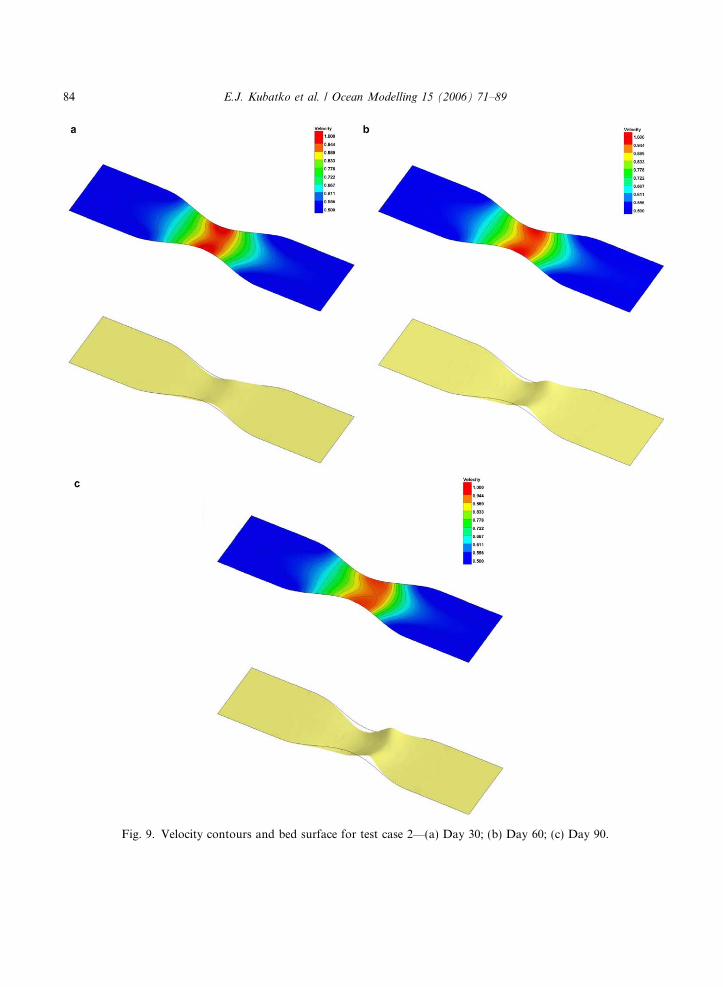
Fig. 9. Velocity contours and bed surface for test case 2—(a) Day 30; (b) Day 60; (c) Day 90.



The velocity throughout the channel varies from approximately 0.50 m/s at the ends of thechannel to approximately 1 m/s in the center of the channel. The bed experiences erosion inthe converging part of the channel due to the increase in the flow velocity. Conversely, in thediverging part of the channel, as the flow velocity decreases, accretion of the sediment occursand a mound or shoal develops in time. It can be noted the scour and accretion patterns occurringin the center of the channel are slightly larger than those occurring toward the sides of the channelacross the width of a given cross section. This can be explained by the fact that the velocity field isnot entirely uniform across the width of the channel with somewhat higher velocities occurring inthe center. These small variations in the velocity field across the width of the channel producevariations in the morphology of the bed across the width of the channel given the fact that thesediment transport is a function of U3. We also note that the velocity field evolves along withthe morphological changes.

Finally, we remark that the computed results of the evolution of the bed compare well quali-tatively to an analytical solution given by Exner (1925) for a problem of the same geometry.Exner�s results, as shown in Fig. 10, are the solution of a simplified model similar to that ofSection 2 but modified accordingly to account for variations in the width of the channel (see Graf,1971 for details). Specifically, it can be seen that the numerical and analytical solutions show thesame general evolution of the bed, i.e. scour in the converging section of the channel and accretionin the diverging section.

Fig. 10. Exner�s analytical solution for the converging channel.


4.3. Test Case 3: Idealized inlet

In this problem, we apply the model to the case of an idealized inlet as shown in Fig. 11. Thedomain consists of a 10 km by 20 km sound connected to the open ocean through an inlet which is1 km wide and 0.5 km long. The open ocean boundary is 20 km from the entrance of the inlet andis 50 km wide. The initial bathymetry in the sound and through the inlet is constant at a depth of5 m. South of the inlet the bathymetry varies linearly from 5 m at the entrance to 14 m at the openocean boundary. The sediment density and median grain size are the same as those specified in theprevious problem. The grid for the problem is also shown in Fig. 11 with the inset showing thedetails in the vicinity of the inlet. The nodal spacing ranges from 100 m near the inlet to 1 kmat the open ocean boundary. The problem is forced with an M2 tide with a 15 cm amplitude whichproduces a maximum current of approximately 1 m/s through the inlet. The time step used for thehydrodynamics is 5 s, and the bed is updated every 50 hydrodynamic time steps. A 28-day simu-lation was run with magnified sediment transport rates in order to enhance the advective processesand accelerate the morphological evolution of the dominant features. Runs with no magnificationof the sediment transport rates produced qualitatively similar results with smaller changes in thebed.

Figs. 12a–d show the time evolution of the bed every 7 days over the 28-day simulation. Notethat larger values in the bed elevation indicate erosion and lower values indicate accretion due tothe fact that the bed is measured as positive downward from the geoid. On day 7, there is notice-able erosion beginning at the southern end of the inlet. Accumulation of the sediment can be seenalong the sides of the inlet and to the south of the inlet indicating the initial formation of an ebbshoal. During flood tide on day 14, it can be seen that there has been significant erosion throughthe throat of the inlet resulting in the initial formation of a flood shoal. It can also be seen that theebb shoal has become more pronounced. By day 21, there are distinct flood and ebb shoals to thenorth and south of the inlet, respectively. There is also additional erosion through the inletfollowing the same pattern as the initial scour. At the end of day 28, there has been significantscour through the entire length of the inlet and the flood and ebb shoals have become even morepronounced. It should be noted that even at this level of coarse grid resolution the model capturesthe main morphological changes one expects to observe in tidally dominated coastal inlets (see forexample Hayes, 1980).

Fig. 11. (a) Computational grid for the idealized inlet of test case 3 and (b) details of the grid in the vicinity of the inlet.

Fig. 12. Evolution of the bed in the vicinity of the inlet over the 28-day simulation—(a) Day 7, (b) Day 14, (c) Day 21,and (d) Day 28.


5. Summary and future work

In this paper, we have presented a new unstructured grid morphodynamic model which makesuse of the existing ADCIRC finite element hydrodynamic model and a new DG finite element sed-iment transport/morphological model. Specific details were given on the implementation of theDG method, and the model was shown to produce good results in three idealized test cases. Inthe first test case it was verified, through the use of the Exner model, that the method achievessecond-order convergence in space. Additionally, it was demonstrated how the DG method canaccurately capture steep gradients in the bathymetry without the introduction of spurious spatialoscillations. The second and third test cases demonstrated how the full morphodynamic modellingsystem can be used to predict medium-term morphological changes of the bed in channels andtidally dominated coastal inlets.


We conclude with some comments on the current development of this morphodynamic model-ling system, in terms of both physical and numerical features that will be implemented. In thispaper, we have only considered sediment transport due to currents. However, in many coastal sce-narios short waves, which interact with the current through the introduction of radiation stressterms in the momentum equations, can be the dominant force in the sediment transport process.Therefore, future work will involve coupling a wave model component into the modelling systemto include the effects of waves in both the hydrodynamics and sediment transport processes.Numerically, as was previously indicated, the present model is only one component of a suiteof DG models that are currently being developed. Other DG model components will include a2DDI DG hydrodynamic model (see Kubatko et al., in preparation) and 2DDI DG transportmodels for salinity and temperature. In many applications, these models will be used in advectiondominated flow scenarios such as coastal inlets. The DG method is particularly advantageous forthese types of situations.

Acknowledgment

This work was supported by the US Army Engineer Research and Development Center undercontracts DACW 42-00-C-0006 and W912HZ-05-0022 under the Coastal Inlets Research Pro-gram with Dr. Nicholas Kraus as technical leader and Ms. Mary Cialone as principal investigator.

References

Blain, C.A., Westerink, J.J., Luettich, R.A., 1994. The influence of domain size on the response characteristics of ahurricane storm surge model. Journal of Geophysical Research 99 (C9), 18467–18479.

Camenen, B., Larson, M., 2005. A general formula for non-cohesive bed load sediment transport. Estuarine, Coastal,and Shelf Science 63 (1–2), 249–260.

Cockburn, B., Shu, C.-W., 1998. The Runge–Kutta discontinuous Galerkin finite element method for conservation lawsV: multidimensional systems. Journal of Computational Physics 141 (2), 199–224.

Cockburn, B., Shu, C.-W., 2001. Review article: Runge–Kutta discontinuous Galerkin methods for convection-dominated problems. Journal of Scientific Computing 16 (3), 173–261.

Crouzeix, M., Raviart, P.-A., 1973. Conforming and nonconforming finite element methods for solving the stationaryStokes equations I. RFAIRO: Analyse numerique 7 (R-3), 33–76.

Dawson, C., Sun, S., Wheeler, M.F., 2004. Compatible algorithms for coupled flow and transport. Computer Methodsin Applied Mechanics and Engineering 193 (23–26), 2565–2580.

De Vriend, H.J., Zyserman, J., Nicholson, J., Roelvink, J.A., Pechon, P., Southgate, H.N., 1993. Medium-term 2DHcoastal area modeling. Coastal Engineering 21 (1–3), 193–224.

Dubiner, M., 1991. Spectral methods on triangles and other domains. Journal of Scientific Computing 6 (4), 345–390.Exner, F.M., 1925. Uber die wechselwirkung zwischen wasser und geschiebe in flussen. Sitzungsberichte der Akademie

der Wissenschaften Wien. 165 (3–4), 165–203.Graf, W.H., 1971. Hydraulics of Sediment Transport. McGraw-Hill Book Company, New York.Hayes, M.O., 1980. General morphology and sediment patterns in tidal inlets. Sedimentary Geology 26 (1–3), 139–156.Henderson, F.M., 1966. Open Channel Flow. MacMillan Publishing Company, New York.Iskandarani, M., Levin, J.C., Choi, B.-J., Haidvogel, D.B., 2005. Comparision of advection schemes for high-order h–p

finite element and finite volume methods. Ocean Modelling 10 (1–2), 233–252.Johnson, Hakeem K., Zyserman, Julio A., 2002. Controlling spatial oscillations in bed level update schemes. Coastal

Engineering 46 (2), 109–126.


Kinnmark, I., 1986. The Shallow Water Wave Equations: Formulation, Analysis, and Application. Lecture Notes inEngineering. Springer-Verlag, New York.

Kubatko, E.J., Westerink, J.J., Dawson, C., in preparation. hp discontinuous Galerkin methods for advectiondominated problems in shallow water flow.

Luettich, R.A., Westerink, J.J, 2004. Formulation and Numerical Implementation of the 2D/3D ADCIRC finiteelement model version 44.XX. Available from: <http://www.marine.unc.edu/C_CATS/adcirc/adcirc_theory_2004_05_14.pdf>.

Lynch, D.R., Gray, W.G., 1979. A wave equation model for finite element tidal computations. Computers and Fluids 7(3), 207–228.

Mukai, A., Westerink, J.J., Luettich, R.A., Mark, D.J. 2002. A tidal constituent database for the western north AtlanticOcean, Gulf of Mexico and Caribbean Sea. Technical Report, US Army Engineer Research and DevelopmentCenter, Vicksburg MS, Report ERDC/CHL TR-02-24.

Nicholson, J., Broker, I., Roelvink, J.A., Price, D., Tanguy, J.M., Moreno, L., 1997. Intercomparision of coastal areamorphodynamic models. Coastal Engineering 31 (1–4), 97–123.

Reed, W.H., Hill, T.R., 1973. Triangular mesh methods for the neutron transport equation. Technical Report LA-UR-73-479, Los Alamos Scientific Laboratory.

Sleath, J.F.A., 1984. Sea Bed Mechanics. John Wiley & Sons, New York.Soulsby, R., Whitehouse, R., 1997. Threshold of sediment motion in coastal environment. Proceedings Pacific Coasts

and Ports 1997 Conference. University of Canterbury, Christchurch, New Zealand, pp. 149–154.Westerink, J.J., Feyen, J.C. , Atkinson, J.H., Luettich, R.A., Dawson, C.N., Powell, M.D., Dunion, J.P., Roberts, H.J.,

Kubatko, E.J., Pourtaheri, H., in review. A new generation hurricane storm surge model for southern Louisiana.Bulletin of the American Meteorological Society.

Westerink, J.J., Luettich, R.A., Muccino, J.C, 1994. Modeling tides in the western north Atlantic using unstructuredgraded grids. Tellus 46A, 178–199.

http://www.marine.unc.edu/C_CATS/adcirc/adcirc_theory_2004_05_14.pdf

http://www.marine.unc.edu/C_CATS/adcirc/adcirc_theory_2004_05_14.pdf

An unstructured grid morphodynamic model with a ...coast/reports_papers/2006-OM-KWD.pdfAn...

Documents

Transcript of An unstructured grid morphodynamic model with a ...coast/reports_papers/2006-OM-KWD.pdfAn...