An Overview of Methods in Linear Least-Squares Regression

Sophia Yuditskaya

MAS.622J Pattern Recognition and Analysis

November 4, 2010

Agenda

• Simple Linear Regression

– Deriving the model

– Evaluating the model

• Regression with Factor Analysis

– Principal Components Regression

– Partial Least Squares Regression

• In-depth Application Example

Data

Goal: Fit a curve to the data

variablesdependent #

st variableindependen #

samples #

m

k

n

kn

predictorsX

mn

responseY

Linear Regression

Y XB EVariance unexplained by regression

Regression coefficients

Offsets (a.k.a. “residuals”)

Simpler analytic formGeneralizes better to polynomial fitting

Least-squares Fitting

• Best fit line:

• Minimizing sum of squares of the vertical offsets:

• Finding the minimum:

(V 2)

ak

0

V 2 [yi f (xi, a0, a1)]2

i1

n

f (x, a0, a1) a0 a1x

Linear Least-Squares Fitting

f (a0,a1) a0 a1x

V 2(a0, a1) [y i (a0 a1x i)]2

i1

n

(V 2)

a0

2 [y i (a0 a1x i)] 0i1

n

(V 2)

a1

2 [y i (a0 a1x i)]x i

i1

n

0

y i a0 a1x i 0i1

n

i1

n

i1

n

n

i

n

i

n

i

ii xaay1 1 1

10

n

i

n

i

ii xanay1 1

10

y ix i a0x i a1x i

2 0i1

n

i1

n

i1

n

y ix i a0 x i i1

n

i1

n

a1 x i

2

i1

n

n x i

i1

n

x i

i1

n

x i

2

i1

n

a0

a1

y i

i1

n

y ix i

i1

n

Solving for a0 and a1

Linear Least-Squares Fitting

n x i

i1

n

x i

i1

n

x i

2

i1

n

a0

a1

y i

i1

n

y ix i

i1

n

a0

a1

n x i

i1

n

x i

i1

n

x i

2

i1

n

1

y i

i1

n

y ix i

i1

n

a b

c d

1

1

ad bc

d b

c a

a0

a1

1

n x i2 x i

i1

n

2

i1

n

x i2

i1

n

x i

i1

n

x i

i1

n

n

y i

i1

n

y ix i

i1

n

1

n x i2 x i

i1

n

2

i1

n

x i2 y i x i y ix i

i1

n

i1

n

i1

n

i1

n

x i y i

i1

n

i1

n

n y ix i

i1

n

Linear Least-Squares Fitting

a0

a1

1

n x i

2 x i

i1

n

2

i1

n

x i

2 y i x i y ix i

i1

n

i1

n

i1

n

i1

n

x i y i

i1

n

i1

n

n y ix i

i1

n

a0

x i

2 y i x i y ix i

i1

n

i1

n

i1

n

i1

n

n x i

2 x i

i1

n

2

i1

n

a1

n y ix i

i1

n

x i y i

i1

n

i1

n

n x i

2 x i

i1

n

2

i1

n

y x i

2 x y ix i

i1

n

i1

n

x i

2

i1

n

nx 2

y ix i

i1

n

nx y

x i2 nx 2

i1

n

Alternate Perspective

xaya

x

yx

xnx

yxnxy

an

i

i

n

i

ii

10

1

22

1

1)var(

),cov(

y i a0 a1x i 0i1

n

i1

n

i1

n

n

i

n

i

n

i

ii xaay1 1 1

10

xaay

n

xa

n

na

n

yn

i

i

n

i

i

10

1

1

01

n

i

ii

n

i

ii

xaaya

V

xaayaaV

1

10

0

2

1

2

1010

2

0)]([2)(

)]([),(

How Well Does Our Model Fit?

• Proportion of variability in Y that is explained

– Coefficient of Determination

– Correlation Coefficient

)var()var(

),cov()(

12

1

2

1

2

102

yx

yx

yy

xaay

rn

i

i

n

i

ii

)()(

),cov(

)var()var(

),cov( 22

ystdevxstdev

yx

yx

yxrr

Problem of Overfitting

• Fitting true patterns or noise?

# Predictors/Features

# Samples

Overfitting

Underfitting Overfitting

Real-World Data

• Constrained sample size– Data collection can be challenging, expensive

• e.g. Manual human annotation

– Outliers, inconsistencies, annotator disagreements• Unreliable for modeling, thrown out

• Can be highly multidimensional– Lots of features (i.e. predictor variables)

• Multicollinearity– Some predictors are highly correlated with others– Creates noise in the data

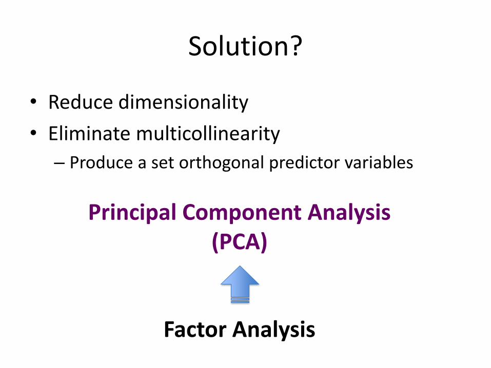
Solution?

• Reduce dimensionality

• Eliminate multicollinearity

– Produce a set orthogonal predictor variables

Principal Component Analysis (PCA)

Factor Analysis

Factor Analysis

Given predictors X, response Y

Goal: Derive a model B such that Y=XB+E, with factor analysis to reduce dimensionality

1. Compute new factor (i.e. “component”) space W

2. Project X onto this new space to get factor scores:

T = XW

3. Represent the model as:

Y = TQ+E = XWQ+E

…where B = WQ

Principal Components Regression (PCR)

• Applies PCA to predictors prior to regression

• Pros:

– Eliminates collinearity orthogonal space

– Produces model that generalizes better than MLR

• Cons:

– May be removing signal & retaining noise

– How to retain the predictors X that are most meaningful in representing response Y?

Partial Least Squares Regression (PLS)

• Takes into account Y in addition to X

• A different kind of Factor AnalysisRecall, T=XW…

– PCR: W reflects var(X)

– PLS: W reflects cov(X, Y)

• Multiple Linear Regression (MLR) vs. PCR vs. PLS– MLR maximizes correlation between X & Y

– PCR captures maximum variance in X

– PLS strives to do both by maximizing cov(X, Y)

PLS Factor Analysis

• Two iterative methods

– NIPALS Nonlinear Iterative Partial Least Squares• Wold, H. (1966). Estimation of principal components and related models

by iterative least squares. In P.R. Krishnaiaah (Ed.). Multivariate Analysis. (pp.391-420) New York: Academic Press.

– SIMPLS more efficient, optimal result

• Supports multivariate Y• De Jong, S., 1993. SIMPLS: an alternative approach to partial least squares

regression. Chemometrics and Intelligent Laboratory Systems, 18: 251–263

SIMPLS

X on Yof tscoefficien regression PLS

+= that such for Y,matrix loadings Factor

+= that such X,for matrix loadingsFactor

matrix scoresfactor PLS

= that such X,for matrix Weight

nm

emptyB

ETQYcn

emptyQ

FTPXcm

emptyP

cs

emptyT

XWTcm

emptyW

T

T

Unexplained variance in X

Unexplained variance in Y

factor tocomponents #

variablesresponse #

variablespredictor #

samples #

c

n

m

s

ms

predictorsX

ns

responseY

Inp

uts

Ou

tpu

ts t

o b

e c

om

pu

ted

loop end

)(normalize

of column into store

of column into store

of column into store

ofr eigenvectodominant

1,...,=for

1

1

1

1

1

1

1

11

hhh

T

hhhh

T

hhhh

h

hh

hhh

h

T

hh

hhh

h

hh

hh

T

hh

hhh

h

T

hh

ACA

ppMM

vvCC

v

vv

pCv

QhwAq

PhwMp

Whc

ww

wMwc

qAw

AAq

ch

A0 XTY

M0 XT X

C0 I

P, Q,W already assembled, iteratively

Compute T XW

Compute B WQT

c # components to factor

T [empty] PLS factor scores matrix

W empty Weight matrix for X such that T = XW

P empty Factor loadings matrix for X, such that X = TP + F

Q empty Factor loadings matrix for Y, such that Y = TQ + E

B [empty] PLS regression coefficients of Y on X

Finally…

Application Example

Automatic Vocal Recognition of a Child’s Perceived Emotional State within the Speechome Corpus

Sophia Yuditskaya

M.S. Thesis (August 2010)

MIT Media Laboratory

The Human Speechome Project

The Human Speechome Project

Recording Statistics

• Birth to age three

• ~ 9.6 hours per day

• 70-80% of child’s waking life

• Over 230,000 hours of A/V recordings

Speechome: A New Kind of Behavioral Data

• Ecologically Valid– Familiar home environment– Child-caretaker interaction– Real daily life situations

• Ultra-dense, longitudinal– Comprehensive record– Insights at variety of time scales

• (e.g.) Hourly, Daily, Weekly, Monthly, Yearly• Up to millisecond precision

Challenges

Previous & Ongoing Efforts

Transcribed SpeechSpeaker ID

Movement TrajectoriesHead Orientation

Child Presence

Speechome Metadata

Thesis Goal

Transcribed SpeechSpeaker ID

Movement TrajectoriesHead Orientation

Child Presence

Speechome Metadata

Child’sPerceivedEmotional

State

Child’sEmotional

State

Thesis Goal

Transcribed SpeechSpeaker ID

Movement TrajectoriesHead Orientation

Child Presence

Speechome Metadata

Child’sPerceivedEmotional

State

Questions for Analysis

• Developing a Methodology– How to go about creating a model for automatic vocal recognition

of a child’s perceived emotional state?

• Evaluation– How well can our model simulate human perception?

• Exploration– Socio-behavioral

• Do correlations change in social situations or when the child is crying, babbling, or laughing?

– Dyadic • How much does proximal adult speech reflect the child’s emotional state?

• Do certain caretakers correlate more than others?

– Developmental• Are there any developmental trends in correlation?

Methodology

RepresentingEmotional State

Emotional State = <valence (mood), arousal (energy)>

Ground Truth Data Collection

Data Collection Methodology

• Annotation interface– Modular, configurable– Streamlined for efficient annotation– Direct streaming Speechome A/V

• Supporting infrastructure– Administrative tool– Database

• Questionnaire

• Data mining strategies to minimize annotation volume

• Hired & supervised annotators (UROPs)

Annotation Interface

Annotation Interface

Minimizing Annotation Volume

• Longitudinal Sampling strategy– 2 full days / mo: months 9-15

– 1 full day / 3 mo: months 15-24

• Filter using existing metadata– Detected speech + Child presence

– Speaker ID (machine learning solution)

Speaker ID

<Speaker Label, Confidence Value>

5 Speaker Categories:

• Child• Mother• Father• Nanny• Other – e.g. Toy sounds, sirens, speakerphone

Filtering by Speaker ID

<Speaker Label, Confidence Value>

5 Speaker Categories:

• Child Keep all• Mother• Father• Nanny• Other – e.g. Toy sounds, sirens outside, speakerphone

Apply Filtering

Problem: choose appropriate confidence thresholds-Above the threshold Filter out-Below the threshold Keep

Filtering by Speaker ID

Criteria: (in order of priority)1. Maximize Sensitivity: % child vocalizations retained 2. Minimize (1- Specificity): % irrelevant clips retained

1-Specificity

Filtering by Speaker ID

• 22% reduction in volume

• Saved roughly 87 hours of annotation time

Annotators

Inter-Annotator Agreement

• P(Agreement)– Does not account for random agreement

• P(Error)– Probability of two annotators agreeing by chance

• Cohen’s Kappa

Poor agreement = Less than 0.20

Fair agreement = 0.20 to 0.40

Moderate agreement = 0.40 to 0.60

Good agreement = 0.60 to 0.80

Very good agreement = 0.80 to 1.00

)(1

)()(

ErrorP

ErrorPAgreementP

Questions

• What is the Nature of the vocalization?» Crying, Laughing, Bodily, Babble, Speech, Other Emoting

• Does it occur during a Social situation?

• Rate its Energy from 1 to 5» 1 = Lowest energy, 3 = Medium, 5 = Highest Energy

• Rate the child’s Mood from 1 to 5» 1 = Most negative, 3 = Neutral, 5 = Most positive

Rating Scale Variants

• Original 5-point scale: {1, 2, 3, 4, 5}5pt

• Collapsed 3-point scale: {1, 2, 3}3pt

– Version A

– Version B

• Expanded 9-point scale: {1, 1.5, 2, 2.5, 3, 3.5, 4, 4.5, 5}9pt

– { Disagreed by 1 point }5pt { Agreed with average value }9pt

Agreement Analysis

Poor agreement = Less than 0.20Fair agreement = 0.20 to 0.40Moderate agreement = 0.40 to 0.60Good agreement = 0.60 to 0.80Very good agreement = 0.80 to 1.00

Post-processing

• Generated agreement indexes

• Pruned noise & overlapping adult speech

• Extracted audio clips from Speechome corpus

– Pruned child vocalizations

– Adult speech surrounding each voc

• 30 sec window before, after

Feature Extraction

Features

• Computed 82 acoustic features

• Praat

Final Dataset for Analysis

• 112 subsets x 5 feature sets = 560 models

For each sample,feature sets were computed from:

(1) The child vocalization

(2) Adult speech before the vocalization

(3) Adult speech after “

(4) Adult speech surrounding “

(5) All of the above combined

Building the Model

What is Best for Our Data?

• Highly multivariate input– 82 features, 328 combined

• Multivariate output: <mood, energy>

• Small and widely varying sample sizes

Dangers: Overfitting, Statistical Shrinkage

For each sample,feature sets were computed from:

(1) The child vocalization

(2) Adult speech before the vocalization

(3) Adult speech after “

(4) Adult speech surrounding “

(5) All of the above combined

Modeling Alternatives

• Multivariate Linear Regression– Supports only univariate output– Susceptible to overfitting

• Principal Components Regression (PCR)– Internal factor analysis (PCA) of input variables

• Reduces dimensionality• Guards against overfitting

• Partial Least Squares Regression– Internal factor analysis includes output variables– Superior to PCR

• Classification accuracy• Generalizability• Robustness to overfitting, sample size effects

PLS Regression Procedure

• Matlab: plsregress(X, Y, nComp, ‘cv’, 10)

X = matrix of input variables

Y = matrix of output variables

nComp = # PLS components to retain

• 10-fold cross validation

• Procedure1. Derive optimal nComp

2. Apply optimal nComp to get final model

3. Evaluate Performance

Deriving Optimal nComp

1. Run plsregress with nComp ≥ 50

2. Plot Mean Squared Error (MSE) vs. # PLS Components

3. Minimum MSE gives optimal nComp

n # samples

p # input variables

BjRegression Coefficient for feature j

Yi

Vector of multidimensional output values for sample i

xijInput value for feature j in sample I

_

Y Sample mean of output data

q # Components

Measuring Model Performance

• R-squared– How well the regression line

approximates the data

• Adjusted R-squared– Normalizing for sample size

and # Components

Interpreting 2

adjR

Cohen, J. (1992) A power primer. Psychological Bulletin 112, 155‐159.

Harlow, L. L. (2005) The Essence of Multivariate Thinking. Mahwah, NJ: Lawrence Erlbaum Associates, Inc.

Results

Results by Socio-Behavioral Context

• Child & Combined: 0.54 to 0.6

– High performing models• Very large effect size >> 0.26

– Consistent across socio-behavioral contexts

• Social situations bring out slight increase

• Child laughing outlier: a mystery

• Adult speech

– Matters…

• Medium effect size (≥ 0.13) in many cases

– …but not too much!

• Small effect sizes elsewhere

• Combined improves only slightly over child.

Dyadic Comparisons

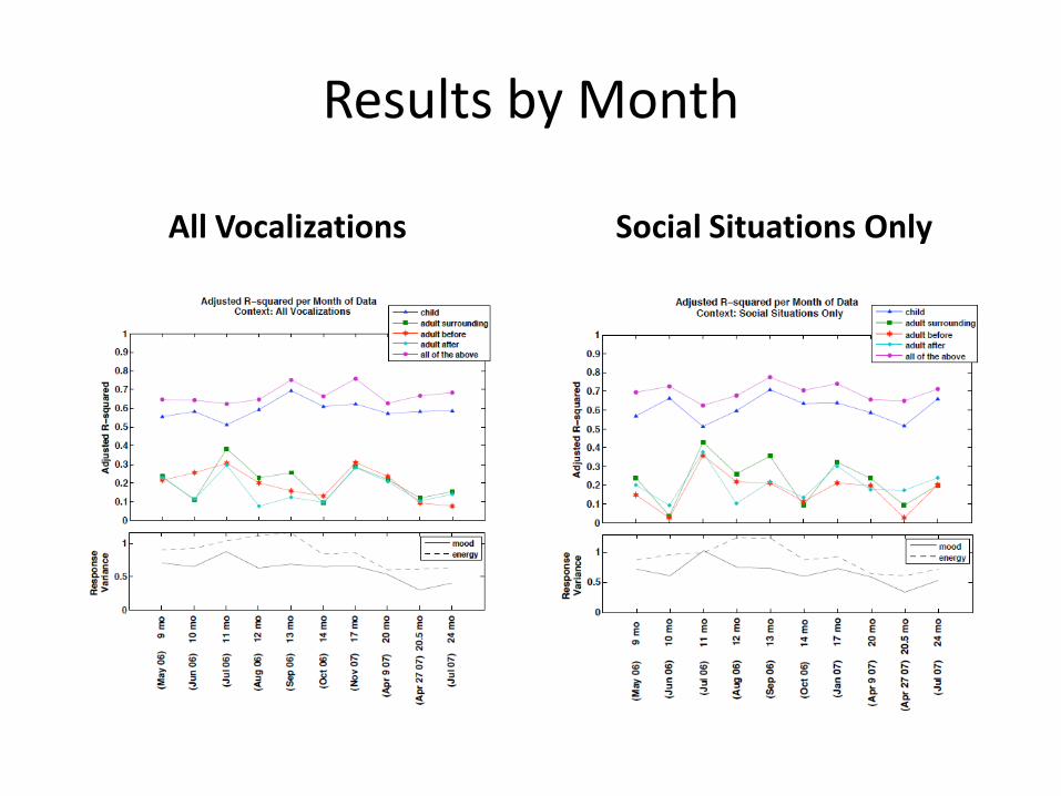
Results by Month

All Vocalizations Social Situations Only

Better to Build Monthly Models

On average, monthly models outperform time-aggregate models

Interesting Progressions

Future considerations

• Do we really need meticulously annotated vocalizations?– Repeat analysis with noisy auto-detected

“speech” segments

• Do the results/trends generalize?– Children can be more or less inhibited

– Repeat analysis with forthcoming new Speechome datasets

Recommended Reading

• Geladi & Kowalski (1986) Partial least-squares regression: a tutorial. Analytica Chimica Acta, 185: 1-17

• Wold, H. (1966). Estimation of principal components and related models by iterative least squares. In P.R. Krishnaiaah (Ed.). Multivariate Analysis. (pp.391-420) New York: Academic Press.

• De Jong, S., 1993. SIMPLS: an alternative approach to partial least squares regression. Chemometrics and Intelligent Laboratory Systems, 18: 251–263

• http://mathworld.wolfram.com/LeastSquaresFitting.html

• Matlab tutorial comparing PCR and PLS:

– http://www.mathworks.com/products/statistics/demos.html?file=/products/demos/shipping/stats/plspcrdemo.html

Thank you!