AN OVERVIEW OF IMPROVED PROBABILISTIC...
160
AN OVERVIEW OF IMPROVED PROBABILISTIC METHODS FOR STRUCTURAL REDUNDANCY ASSESSMENT OF INDETERMINATE TRUSSES BY JULIEN RENE PATHE DEPARTMENT OF CIVIL, ARCHITECTURAL AND ENVIRONMENTAL ENGINEERING Submitted in partial fulfillment of the requirements for the degree of Master of Science in Civil Engineering in the Graduate College of the Illinois Institute of Technology Approved _________________________ Adviser Chicago, Illinois July 2012
Transcript of AN OVERVIEW OF IMPROVED PROBABILISTIC...

AN OVERVIEW OF IMPROVED PROBABILISTIC METHODS FOR STRUCTURAL
REDUNDANCY ASSESSMENT OF INDETERMINATE TRUSSES
BY
JULIEN RENE PATHE
DEPARTMENT OF CIVIL, ARCHITECTURAL
AND ENVIRONMENTAL ENGINEERING
Submitted in partial fulfillment of the
requirements for the degree of
Master of Science in Civil Engineering
in the Graduate College of the
Illinois Institute of Technology
Approved _________________________
Adviser
Chicago, Illinois
July 2012


iii
ACKNOWLEDGEMENT
It would not have been possible to write this thesis without the help and support
of the caring people surrounding me.
Foremost, I would like to express my sincere gratitude to my advisor, Dr. Jamshid
Mohammadi, whose patience, enthusiasm and knowledge were continuous supports
throughout this research.
I would like to thank the many professors to whom I am indebted for providing a
stimulating learning environment. I am especially grateful to the professors of the
National Institute of Applied Science in Strasbourg, France, with whom I spent four
enriching years. Special thanks go to the Civil, Architectural and Environmental
Engineering faculty of the Illinois Institute of Technology which made my final year an
unforgettable learning experience.
Lastly, I wish to thank my family and especially my mother who realized before
me that learning English could take me to wonderful journeys, so was this all year.

iv
TABLE OF CONTENTS
Page
ACKNOWLEDGEMENT ....................................................................................... iii
LIST OF TABLES ................................................................................................... vi
LIST OF FIGURES ................................................................................................. vii
ABSTRACT ............................................................................................................. x
CHAPTER
1. INTRODUCTION .............................................................................. 1
1.1 Objectives ............................................................................ 1
1.2 Importance ........................................................................... 1
1.3 Scope .................................................................................... 2
2. REVIEW OF RELATED WORK ...................................................... 3
2.1 Definitions ............................................................................ 3
2.2 Importance of redundancy ................................................... 13
2.3 Criterion for a realistic evaluation of redundancy ............... 17
2.4 Present ways of considering redundancy in design codes ... 23
3. PRESENTATION OF A CLASSICAL METHOD TO COMPUTE
THE PROBABILITY OF FAILURE OF A STRUCTURE ............... 34
3.1 Existing methods .................................................................. 34
3.2 Structural analysis for trusses .............................................. 36
3.3 Classical method to compute the probability of failure of a
structure using failure paths .......................................................... 51

v
CHAPTER Page
4. PROPOSED METHOD TO COMPUTE THE PROBABILITY OF
FAILURE OF A STRUCTURE ......................................................... 67
4.1 Introduction .......................................................................... 67
4.2 The limit state model .......................................................... 67
4.3 Probability calculations for a linear limit state ................... 74
4.4 The load continuity hypothesis ............................................ 83
4.5 The most central failure point .............................................. 92
4.6 Probability calculations for multiple linear limit states ....... 95
4.7 Material post-failure behavior .............................................. 112
4.8 The linear limit state approximation .................................... 116
4.9 Framework of analyses ........................................................ 122
4.10 Probability of failure for the system .................................... 123
4.11 Concluding remarks ............................................................. 127
5. ILLUSTRATIVE EXAMPLE ............................................................ 129
5.1 Study of the intact structure ................................................. 129
5.2 Study of the structure with the member 1 failed .................. 134
5.3 Study of the structure with the member 3 failed .................. 139
5.4 Structure probability of failure ............................................. 143
6. SUMMARY AND CONCLUSIONS
6.1 Summary .............................................................................. 146
6.2 Recommendations for further studies .................................. 147
BIBLIOGRAPHY .................................................................................................... 148

vi
LIST OF TABLES
Table Page
5.1 Probability of member failure for the intact structure ................................ 134
5.2 Most central failure point for the intact structure ....................................... 134
5.3 Probability of member failure for the structure with member 1 failed ...... 138
5.4 Probability of member failure for the structure with member 3 failed ...... 143
5.5 Probability of occurrence of failure paths .................................................. 144

vii
LIST OF FIGURES
Figure Page
2.1 Truss structure with a mechanism and an indeterminate substructure ......... 5
2.2 Comparison of two structures with one degree of redundancy .................. 5
2.3 Internal and external indeterminate structures ............................................ 6
2.4 Load path .................................................................................................... 7
2.5 Stress-strain constitutive relations .............................................................. 8
2.6 Failure paths ............................................................................................... 10
2.7 Failure paths tree ........................................................................................ 11
2.8 Damage curve example .............................................................................. 14
2.9 Origins of the risks ..................................................................................... 16
2.10 Venn diagram of the load and structure space ........................................... 23
3.1 Global and local coordinate systems .......................................................... 37
3.2 Degrees of freedom, joint load vector and reaction vector ........................ 40
3.3 Member forces and displacement in the local coordinate system .............. 42
3.4 Member forces and displacement in the global system and relationship
between the local and global coordinate system ........................................ 43
3.5 Displacement vector, load vector and reaction vectors ............................... 46
3.6 Assembling of the structure stiffness matrix using numbering techniques 50
3.7 Parallel and series systems ......................................................................... 53
3.8 Member probability of failure associated with Z ....................................... 58
4.1 Von-Mises Criterion limit state .................................................................. 69
4.2 Linear limit state ......................................................................................... 71
4.3 Non-convex safe set ................................................................................... 71

viii
Figure Page
4.4 Non-convex failure set for a concrete column ........................................... 72
4.5 Multiple linear limit state in 2-dimensional space .................................... 73
4.6 Multiple linear limit states in 3-dimensional space .................................... 74
4.7 Geometric interpretation of the reliability index in the normalized space . 77
4.8 Reliability index β and safety margin distribution ..................................... 82
4.9 Loading evolution function in the subset L ................................................ 85
4.10 Reliability model with inconsistent limit states ......................................... 87
4.11 Corrected reliability model without inconsistent limit states ..................... 88
4.12 Reliability model with unnecessary limit states ......................................... 89
4.13 Corrected reliability model without unnecessary limit states .................... 90
4.14 Most central failure point ........................................................................... 93
4.15 Most central failure points for multiple limit states ................................... 94
4.16 Multiple linear limit states before shaping ................................................. 100
4.17 Multiple linear limit states after shaping and straight load evolution
function ..........................................................................................................100
4.18 Perfectly correlated limit states .................................................................. 102
4.19 Independent limit states .............................................................................. 102
4.20 Joint failure set for the limit stat I and the limit state j ............................... 106
4.21 Failure set corresponding to the probability ( ) ( ) .............. 106
4.22 Failure set corresponding to the probability ( ) ( ) ............. 107
4.23 Geometric interpretation of the correlation coefficient .......................... 108
4.24 Linear elastic – perfectly plastic model ...................................................... 113
4.25 Linear elastic – linear work hardening model ............................................ 116

ix
Figure Page
4.26 Convex safe set ........................................................................................... 117
4.27 FORM approximation ................................................................................ 117
4.28 SORM approximation ................................................................................ 118
4.29 Linear limit state approximation and variables scatter ............................... 121
4.30 Framework of the proposed method ........................................................... 123
4.31 Successive mutually exclusive sets ............................................................ 126
5.1 Geometry of the structure and member numbers ....................................... 129
5.2 Results of the structural analysis for the intact structure ............................ 130
5.3 Member strengths ....................................................................................... 131
5.4 Limit states in the normalized space for the intact structure ...................... 132
5.5 Consistent limit states for the intact structure ............................................ 133
5.6 Results of the structural analysis for the structure with failed member 1 .. 135
5.7 Forces in members caused by the member 1 plastic force ......................... 135
5.8 Limit states in the normalized space for the structure with failed member 1 137
5.9 Consistent limit states for the structure with failed member 1 ................... 138
5.10 Results of the structural analysis for the structure with failed member 3 .. 139
5.11 Forces in members caused by the member 3 plastic force ......................... 140
5.12 Limit states in the normalized space for the structure with member 3 failed 141
5.13 Consistent limit states for the structure with member 3 failed ................... 142
5.14 Failure paths tree for the example structure ............................................... 145

x
ABSTRACT
The redundancy of a structure refers to the extent of strength that is not
considered in design. For an indeterminate structure a member failure does not
necessarily induces the loss of integrity or functionality of the structure; rather it will
affect its potential for safely carrying any future load. Numerous methods have been
introduced in structural reliability literature to measure and implement the redundancy in
design. However, in accordance with the semi-probabilistic approach of the codes which
aim to develop design method providing consistent level of redundancy within the
structure, the probability of failure of the structure has been proposed and is widely used
as a redundancy measure. A classical method to compute the probability of failure of the
structure based on failure paths is presented as a reference in this thesis. However,
although extensively used, this method has major shortcomings which may lead to a
misrepresentation of the structure redundancy. By using a geometric representation of
members’ limit states associated with a loading regime, the research presented herein
proposes an improved method for structural redundancy estimation that may be helpful to
overcome problems associated with approximations and inconsistencies inherent in
classics methods. Specific assumptions and/or procedures considered in the proposed
method are described below.
(1) An approximation is given to make the events of member failures mutually
exclusive.
(2) Geometric calculations are used to determine reliability indices and
conditional reliability indices in order to establish closer bounds for the failure
probability of individual structural members.
xi
(3) System’s failure probability is obtained using the assumption and procedures
outlined in (1) and (2) above.
(4) To further extend the method beyond geometrical redundancy, and to consider
material redundancy, plasticity models commonly used in the structural analyses are
considered in this study.
1
CHAPTER 1
INTRODUCTION
1.1 Objectives
The indeterminacy of a structure refers to the structure capacity to be stable after a
member removal. The strength remaining in the stable damaged structure is called the
reserve strength of the structure and is the measure of the structure redundancy. In the last
thirty years numerous researches have been conducted leading to various different
methods of the reserve strength quantification. Probabilistic methods are now preferred,
because they provide a global description of the structure’s redundancy and they can be
implemented in semi-probabilistic codes. However, the research is still in its early stages
of development; and the proposed methods (as described in this thesis) have many
shortcomings which makes them inapplicable in a code. Indeed, so far, no code
recommends a special approach for indeterminate redundant structures. The purpose of
this study is to contribute to the improvement of these probabilistic methods by taking a
classical method whose framework is widely used among researchers and improve upon
its procedure.
1.2 Importance
The primary importance of measuring redundancy is to enable to design with a
consistent level of risk within the structure. In a semi-probabilistic design every member
is assigned with the same probability of failure. However, the consequences on the
structure integrity or functionality of a member failure are different depending on the
considered member. Instead of designing members with the same level of risk with

2
regard to member failure, a measure of redundancy allows to design with the same level
of risk with regard to the structure’s failure.
The second importance of considering redundancy is the recognition that the
unexpected can occur. This could be the occurrence of a rare event, the occurrence of
poor structure characteristics or a construction fault. Additional safety can be provided to
the structure by designing a system that can transfer load from one member to other
members should one member break. This type of structure is called a fail-safe structure.
On this type of structure the fracture is controlled and repairs are possible.
1.3 Scope
The evaluation of the redundancy described in this study consists of the
following:
A review of related work. Evaluation of the current practices and proposed
method of considering indeterminacy and redundancy.
A detailed presentation of a classical method to compute the probability of failure
of an indeterminate structure. The study of this method enables us to outline its
shortcomings.
A proposed method based on the classical method framework. Strategies are
proposed to overcome the classical method shortcomings.
An application of the proposed method on a simple structure to show how it is
implemented and the results found.

3
CHAPTER 2
REVIEW OF RELATED WORK
2.1 Definitions
Since some of the terms used in literature may have meanings that may not be
clear to this study, the following definitions and nomenclature are used in this thesis for
clarity.
2.1.1 Statically indeterminate structure.
2.1.1.1 Definition. The indeterminacy of a structure is a global characteristic, which
corresponds to the lack of equilibrium equations compared with the number of unknown
internal forces. Generally-speaking, a structural system is stable without a need to have
redundancy. Therefore, redundant internal forces are not necessary to have a stable
system; and such, they can be removed without deteriorating the stability of the system.
In other words, some structural members can be totally removed without compromising
the stability of the entire system. In a redundant system, however, a certain amount of
damage can be tolerated without making the structure unstable. The more the system is
indeterminate the more it can tolerate damage and removal of individual members due to
any failure. However, it is emphasized that individual members may have different levels
of influence on the overall integrity of the system. This is to say that, a system may
geometrically appear to be indeterminate, however, for practical purposes, the same level
of load may cause instability as soon as the member is failed. Thus, an indeterminate
structure, even still stable after damage, may not be able to carry the same amount of load
before damage.

4
2.1.1.2 Degree of static indeterminacy. A simple indicator of indeterminacy is to count
the number of the unknown internal forces minus the total number of equations of
equilibrium. This number is called the degree of indeterminacy. This can be demonstrated
through the following equation:
( ) ( )
Where all variables are non-negative integers as described below:
= forces = number of internal force in each member
= members = number of members
= restraints = number of restraints, i.e., boundary conditions
= equations = number of equilibrium equations per joint
= joints = number of joints
= hinges = number of hinges or other sections force releases
However this indicator is imperfect. Indeed, when applied to the entire structure, a
substructure can present a deficit of unknowns whereas another substructure would
present an excess of unknowns. In that case, the whole structure could be said to be
indeterminate even if a mechanism exists inside the structure. Moreover depending of the
geometry of the structure, by using this indicator a structure can be said to be stable, i.e.,
determinate or indeterminate whereas it is a mechanism (figure 2.1).
As a consequence, this indicator should be used with caution; and since the
stiffness matrix of the entire system may be considered to be a more reliable indicator of
the stability of a structure, the matrix may offer a better indicator of redundancy.

5
Figure 2.1 Truss structure with a mechanism and an indeterminate substructure
Figure 2.2 Comparison of two structures with one degree of redundancy
2.1.1.3 Internal and external degrees of statically indeterminacy. It is possible to
divide degrees of indeterminacy into two categories – these are internal and external
degrees of indeterminacy. The external degree of indeterminacy is the number of
boundary conditions minus the number of global static equilibrium equations (3 for plane
structures, 6 for space structures). The internal degree of indeterminacy refers to the
mechanism
indeterminate
substructure
(a) mechanism (b) stable structure
6
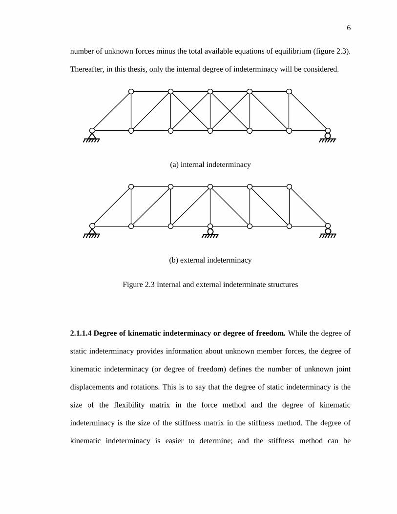
number of unknown forces minus the total available equations of equilibrium (figure 2.3).
Thereafter, in this thesis, only the internal degree of indeterminacy will be considered.
(a) internal indeterminacy
(b) external indeterminacy
Figure 2.3 Internal and external indeterminate structures
2.1.1.4 Degree of kinematic indeterminacy or degree of freedom. While the degree of
static indeterminacy provides information about unknown member forces, the degree of
kinematic indeterminacy (or degree of freedom) defines the number of unknown joint
displacements and rotations. This is to say that the degree of static indeterminacy is the
size of the flexibility matrix in the force method and the degree of kinematic
indeterminacy is the size of the stiffness matrix in the stiffness method. The degree of
kinematic indeterminacy is easier to determine; and the stiffness method can be
7
implemented (in computer assisted structural analyses) in a straightforward manner to
arrive at equations for solving the degrees of freedom.
2.1.2 Fail-Safe structure. A fail-safe condition refers to a type of structure, which in
the event of failure will respond in a way that will cause no harm to the users or
occupants. A proper structural system design is intended to prevent or mitigate unsafe
consequences of a failure and to protect the users or occupants. For example, in a
structural system, an event of safe failure is the local failure of a single member; whereas,
the unsafe consequence may be corresponding to the case when the entire structure
collapses.
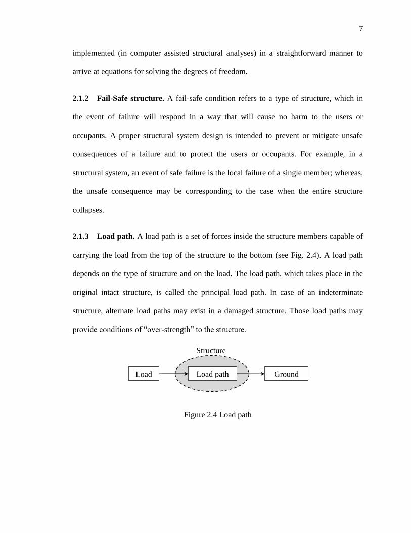
2.1.3 Load path. A load path is a set of forces inside the structure members capable of
carrying the load from the top of the structure to the bottom (see Fig. 2.4). A load path
depends on the type of structure and on the load. The load path, which takes place in the
original intact structure, is called the principal load path. In case of an indeterminate
structure, alternate load paths may exist in a damaged structure. Those load paths may
provide conditions of “over-strength” to the structure.
Figure 2.4 Load path
Load Load path
Structure
Ground

8
2.1.4 Material and geometrical redundancy.
2.1.4.1 Material redundancy. The material redundancy of a structure is the additional
resistance a member (that is considered failed for practical purposes) can provide to the
system. This type of redundancy is provided by the rheology of the material. There are
two types of material redundancy: the displacement-redundancy, the constraint-
redundancy.
The displacement-redundancy enables a failed element of the structure to
accommodate additional displacement whereas the constraint-redundancy enables the
failed element to resist to additional constraint. In general, elements are both
displacement-redundant and constraint-redundant.
The stress-strain constitutive relation of a material describes the material
redundancy. The following diagrams (figure 2.5) provide idealized comprehensive
examples for different types of redundancy.
Figure 2.5 Stress-strain constitutive relations
𝜺 𝜺 𝜺 𝜺
𝝈 𝝈 𝝈 𝝈
(a) (b) (c) (d)

9
The situation denoted by (a) in Figure 2.5 has no redundancy. The situation
denoted by (b) has only a displacement redundancy. The situation denoted by (c) has only
a constraint redundancy. The situation denoted by (d) has both displacement and
constraint redundancy.
2.1.4.2 Geometric redundancy. Geometric redundancy is the ability of a structure, for
which all members are considered without material redundancy, to redistribute the load
among its members when damage to certain members has occurred. Since redundancy is
generally associated with indeterminacy the indeterminacy of at least some parts of the
structure is required to provide alternative load paths. However the degree of static
indeterminacy is not a consistent measure for geometric redundancy. A structure is said
to be geometrically redundant if it possesses at least a few members that are considered
geometrically redundant.
2.1.4.3 System redundancy. A system is said to be redundant if it has some members
which are either geometrically redundant or materially redundant. As described earlier,
material redundancy can be interpreted as the reserve strength of a member itself,
whereas geometric redundancy can be taken as the reserve strength of a structure beyond
point of yield. This distinction between material and geometric redundancy is only
theoretical since both occur in a given structure indistinctively. Indeed, when a member is
considered as failed and starts being materially redundant, its behavior will be modified.
This behavior modification leads to a reorganization of forces in the structure; and as
such, alternative load paths are formed to sustain the loads. At this stage, the geometric
redundancy is then used. Thus the redundancy of a system is the reserve strength
10
available from both material redundancy and geometrical redundancy of member for
preventing failure of an entire structural system upon a failure of a single element.
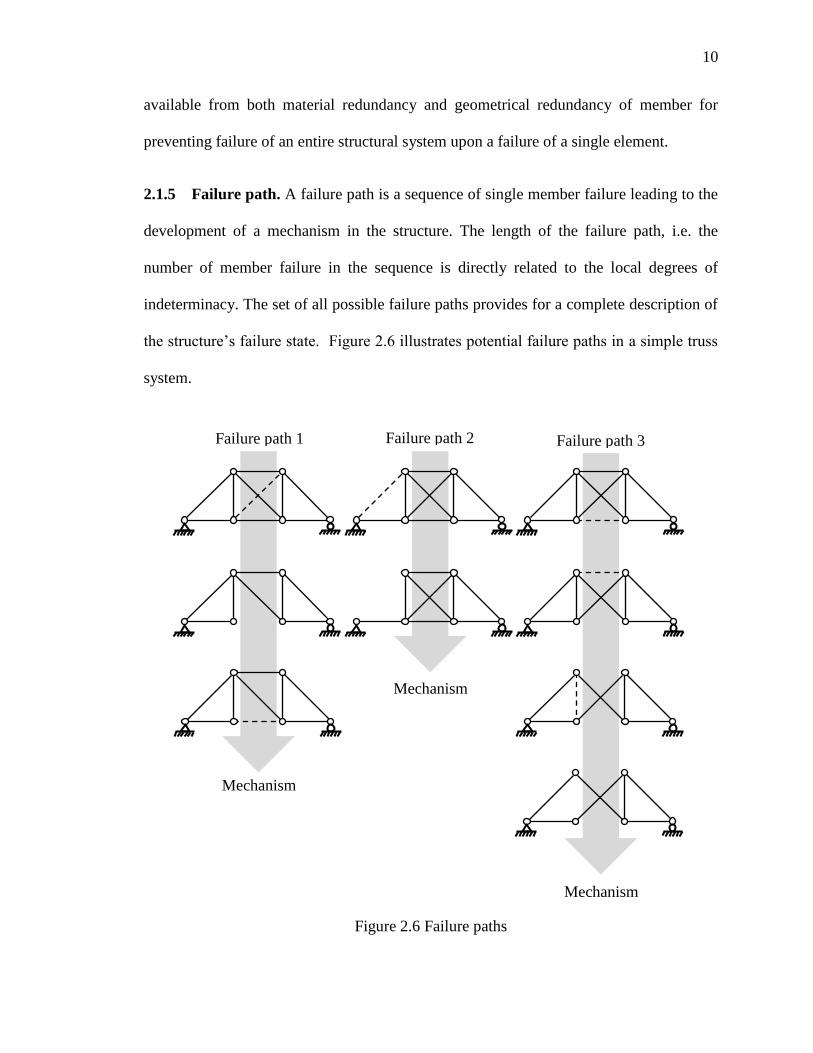
2.1.5 Failure path. A failure path is a sequence of single member failure leading to the
development of a mechanism in the structure. The length of the failure path, i.e. the
number of member failure in the sequence is directly related to the local degrees of
indeterminacy. The set of all possible failure paths provides for a complete description of
the structure’s failure state. Figure 2.6 illustrates potential failure paths in a simple truss
system.
Figure 2.6 Failure paths
Failure path 1 Failure path 2 Failure path 3
Mechanism
Mechanism
Mechanism

11
As seen in figure 2.6, three possible failure paths are present in the structure. It
can be seen that different failure paths have different lengths in terms of the number of
members that need to fail before the formation of a mechanism in the structure. The three
presented failure paths are a non-exhaustive example of the variety of the possible failure
paths. To represent possible failure paths, a tree diagram can be used as shown in figure
2.7.
Figure 2.7 Failure paths tree
1
1
1
2
3
2
3
1
4
3
3
2
Failure of member 3
Collapse caused by the member 2 failure
Other failure paths
12
As a complete representation of all the possible fracture mechanisms, a failure
paths tree enables us to take into account the role of every elements in every given failure
scenario. However, for complex structures, the failure paths tree may not be readily
evident. In these cases, algorithms can be used to generate every failure path with an aid
of a computer program.
2.1.6 The reserve strength. The reserve strength can be linked to the redundancy. As
described earlier, the redundancy is defined as the structure’s capacity in sustaining more
loads after an initial failure. The amount of strength remaining in the structure is called
the reserve strength. Thus, in simple terms, the reserve strength can be considers as a
measure of the redundancy of the structure. However, more definite measures to quantify
the reserve strength are used as described below.
Possible ways to quantify the reserve strength with a deterministic approach:
First a member must be chosen as a candidate to fail. Then a structural analysis on
the damaged structure is conducted. The over strength can be chosen freely as a
characteristic of the damaged structure. For example, one can choose the
maximum load for a given limit deflection, or, one can choose the maximum load
before the failure of the next member. Thus, in the case of a deterministic
approach, the reserve strength can only be a partial measure given a specific
situation
Possible ways to quantify the reserve strength with a probabilistic approach:
The over-strength of a damaged structure is introduced via a probability value.
This value represents the chance of failure and is in fact equal to the probability
that in a specific member the over-strength value is exceeded. For a structural

13
system, this probability value is the probability that the system over-strength is
exceeded or a failure mechanism has taken place. Since this probability can be
computed at any stage when members are failing, the difference between the
probability values from one loading stage to another (as structural degradation
takes place) can be used as a measure for the reserve capacity as discussed later in
this thesis.
2.2 Importance of redundancy
2.2.1 Structure behavior during failure. In current practice, the strength evaluation of
a structure is typically based on using elastic analysis to determine the distribution of load
effects in the members and then checking the ultimate section capacity of those members
against the applied load effects. However, when a failure criterion is used to define the
failure of the entire structure (rather than the failure of a single member), this strength
evaluation may not be accurate. Material redundancy, i.e. ductility, of the components
permits local yielding (especially in most heavily loaded members) and, coupled with
geometric redundancy, enables subsequent redistribution of the internal forces. As a
result, a system can continue to carry additional loading even after one member has
yielded, which has conventionally been adopted as the failure criterion in structural
strength evaluation. This means that a structure with redundancy has additional reserve
strength such that the failure of one element does not result in the failure of the complete
system. The reserve strength is a measure of the redundancy of a system and its capacity
to safely redistribute forces among its members when damage has occurred. When
designing without taking into account the redundancy, one needs to provide for additional
14
safety using stronger structural members. This of course will result in additional costs.
Designing with redundancy potentially enables the engineer to control the fracture
process that leads to failure. This ability of controlling the fracture process is governed by
two main concepts, namely, the reserve strength and the discretization of the failure
process. As explained later, through a probabilistic formulation, these two concepts can
be considered in structural analysis to provide an improved measure describing the
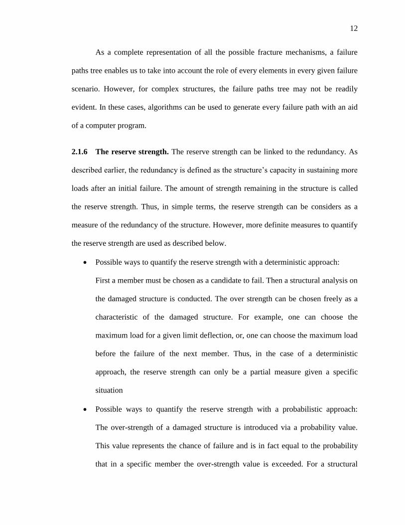
system redundancy. More specifically, these two concepts can be introduced through a
“damage curve” [10]. A damage curve is a relationship between a normalized damage
level and an applied load that produces the damage (see Fig. 2.8). The damage level 0
represents no damage, i.e., no yielding of any member, and 1.0 represents total collapse
of the structure. For cases where the damage is partial, the damage is proportional to the
number of failed members.
Figure 2.8 Damage curve example
Figure 2.8 presents two damage curves of two redundant systems. Structure (a)
spreads out the failure process in five steps; whereas the structure (b) does it in only two
0
0.2
0.4
0.6
0.8
1
Dam
age
ind
ex
Load
(a) (b)
15
steps. System (b) has more reserve strength, i.e., can carry more load, than does structure
(a). Although these two curves provide a description of the discretization of the failure
process and the reserve strength, without further analysis, it will be difficult to determine
the inherent level of safety of each structure through redundancy of which system. A
probabilistic definition of the reserves strength (including the discretization of the failure
process) will be helpful to introduce the problem through probable values of reserved
capacity and thus offer an alternate solution in defining the redundancy and its
significance in defining safety.
To control the fracture process at the design stage, one must know the loads and
its variation in time. Unexpected loads can occur and, as a result, the reserved strength of
the structure may be needed to resist against them. By incorporating an accurate estimate
for redundancy, and designing for a fail-safe condition, the fracture process is controlled
leading to a design with a more consistent level of risk.
2.2.2 Representation of the risk. Designing with redundancy and with an accepted
risk level for collapse is not necessarily leading to a structure that is stronger, but rather
the design will have the capability to account for the fact that an unexpected load can
occur and still a safe level of performance is attained. This could be the occurrence of
rare events such as floods or earthquakes, poor maintenance, human error, unexpected
fatigue cracking, a severe wind storm, etc. By incorporating an accurate estimate of
redundancy, the engineer is able to reduce the damaging effects of occurrences of these
rare events and have a more consistent level of accepted risk.

16
Figure 2.9 Origins of the risks
Hazard potential
Objectively known
Subjectively realized
Taken into account
Risk treatment measures
Adequate measures
Correctly implemented
measures
Accepted risk
Not known
Not realized
Neglected
Not adequate
Wrong
(a) Origins of the risks for a structure with low levels redundancy
Hazard potential
Objectively known
Subjectively realized
Taken into account
Risk treatment measures
Adequate measures
Correctly implemented
measures
Accepted risk
Not known
Not realized
Neglected
Not adequate
Wrong
Accepted risk
Hazards due to human errors – low levels of redundancy
Hazards due to human errors – high levels of redundancy
(b) Origins of the risks for a structure with high levels
redundancy
(c) Risk comparison in function of levels of redundancy

17
Figure 2.9 presents diagrams that depict the relation between risk and redundancy
for a given system. The significance of low and high levels of redundancy on the risk of
failure is demonstrated. A structure with a low level of redundancy, for example, is
designed without recognizing that unexpected loads or service conditions may occur. As
a consequence the hazards due to the unexpected events are relatively severe as oppose to
a structure designed with redundancy. On the other hand, a structure designed with a high
level of redundancy has more consistent level of risk because the accepted risk, which is
decided by the engineer and the structure is accommodated for the risk, is closer to the
risk from hazards due to the unexpected events.
2.3 Criterion for a realistic evaluation of redundancy
Several criteria have been proposed to assess the overall redundancy of a system.
Some relevant studies will be introduced in this section. Then, the criterion that will be
used in the thesis will be introduced.
2.3.1 The deterministic redundancy factor and the redundancy index. The
following discussion is from research by Frangopol and Curley [7]. The deterministic
redundancy factor and the redundancy index consider the effect of damage or failure of a
given component on the system strength in the damaged condition. The structural
residual strength factor is defined as follows:
In which,
is the ultimate strength of the undamaged system

18
is the residual strength of the damaged system
The structural redundancy factor is defined as follows:
This redundancy factor ranges from a value of 1.0 when the damaged structure
has no reserve strength to a value of infinity when the structural damage has no influence
on the reserve strength of the system. The redundancy factor is calculated for each
component. Based on the redundancy factor of various members, the engineer can
identify the important members as those with having the greatest influence on the
reserved strength of the structure.
However, this criterion can only be used as a partial description of redundancy.
Indeed, this factor has some drawbacks:
Every member must be computed independently. It does not provide a global
description of the structure.
The loading must be the same type for every computed member. It does not
enable the engineer to provide a complete description of the loading.
The total redundancy of the structure is not considered. The damaged structured is
considered to be failed when a second member fails: and as such, the
representation of the redundancy is not total but at best partial.
2.3.3 The beta index. A probabilistic measure of the redundancy of a structure based
on the structural redundancy factor proposed Frangopol and Curley [7] is used in this

19
thesis. According to this model, a parameter (referred to as the reliability index) is
introduced as described below.
( ) ( )
( ) ( )
In which,
( ) is the beta index or reliability index of the intact structure
( ) is the reliability index of the damaged structure
The beta index (or reliability index) is the input in the cumulative distribution
function of the standardized normalized distribution. This simple indicates that:
; ( )
In which is the probability of failure (or damage) of the structure. This index
can also be expressed as the difference between the resistance of the structure and the
applied load with the variance of this difference taken as unity. This probabilistic
measure of redundancy ( ) varies between 1 and infinity. Unlike the structural
redundancy factor , ( ) enables us to fully describe the variety in loading. However
there are still two main drawbacks in arriving at an accurate value for the structural
redundancy factor . These are (1) the fact that still the redundancy for each member
must be computed separately; and (2) that the system redundancy so obtained is not
accurately representing the total system redundancy.

20
2.3.3 The successive damage probability. The successive damage probability is also
used to develop a method for redundancy as proposed by Mohammadi, Longinow and
Suen [11]. This method determines the effectiveness of redundant components in a
structural system as the determining factor in defining redundancy. Specific application
presented is for bridges. The method requires the calculation of the probability of
damage to the structural system before and after removal of a redundant component.
Damage is defined as the failure of one or more components; and the probability of
damage of the system is:
( ) (⋃
<
)
In which:
is the event of failure of the individual component
( ) is calculated for the intact structure and then again for the system with one
component failed. The values for ( ) are then compared at each stage after a partial
damge; and, if the results are nearly equal, the structure is considered to have a moderate
degree of redundancy. Continuing with this process, then a second component, in
addition to the first component, is considered failed and a new probability of damage is
calculated. This process continues until the damage probability shows a sudden increase.
This increase indicates that the collapse of the system has become certain. The number of
components removed to result in the collapse stage is a measure of the redundancy of the
system. If, however, ( ) shows a significant increase after removal of a first single

21
member, the system is considered to have no redundancy. A criterion that would limit the
increase of the system probability of damage could be established to provide uniformity
to the method. This approach is a good attempt in providing a method that does not
present the drawbacks of the two first methods. However, this method does not, to some
extent, represent the very accurate estimate of the redundancy, since the process which
leads from the first damaged member to the complete failure of the structure is arbitrary
chosen. Indeed, using this method, the redundancy of a structure depends on the sequence
of member removals. Some members may appear to be more (or less) critical depending
on the failure sequence in which they are involved. Using this method, the probability
formulation is only in computation of the risk of damage and not in the sequence of
member failures leading to the system collapse. A more realistic method would have
provided for a probabilistic approach in the sequence of member failures also.
2.3.4 The probability of failure. In light of the fact that the redundancy computation
using the aforementioned method requires the computation of the probability of failure,
the following provides a brief review of the relevant topics in the theory of probability.
The reliability criterion must be global. It must consider, as much as possible, an
accurate geometry and/or characteristic for the structure and the applied loads
The reliability criterion must be straightforward limiting the need for the engineer
to rely on personal judgment.
The reliability criterion must also be consistent with the safety of the structure;
such that it can be used for ranking structures from those with lesser to those with
higher safety levels.
22
The reliability criterion must be also present a unique representation of the safety
of the system. This means, using the chosen reliability criterion, the analysis must
always result in the same probability of failure.
With regards to these requirements, the rationale for a realistic evaluation of
redundancy will be based on the probability of failure of the structure given the structure
has already been damaged. To evaluate this probability, a probability space and three
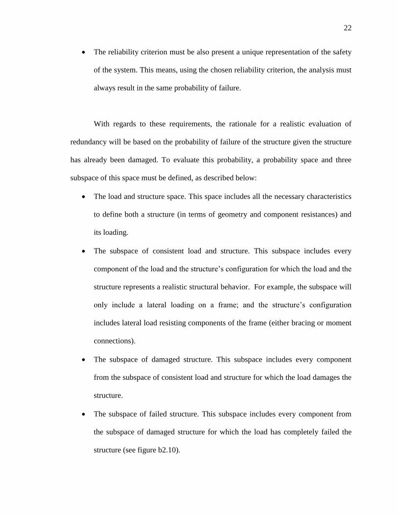
subspace of this space must be defined, as described below:
The load and structure space. This space includes all the necessary characteristics
to define both a structure (in terms of geometry and component resistances) and
its loading.
The subspace of consistent load and structure. This subspace includes every
component of the load and the structure’s configuration for which the load and the
structure represents a realistic structural behavior. For example, the subspace will
only include a lateral loading on a frame; and the structure’s configuration
includes lateral load resisting components of the frame (either bracing or moment
connections).
The subspace of damaged structure. This subspace includes every component
from the subspace of consistent load and structure for which the load damages the
structure.
The subspace of failed structure. This subspace includes every component from
the subspace of damaged structure for which the load has completely failed the
structure (see figure b2.10).

23
Figure 2.10 Venn diagram of the load and structure space
The criterion for the evaluation of redundancy is the probability of failure given
the structure has already been damaged which is the probability of occurrence of a
specific scenario from the subspace of the failed structure, when considering only the
subspace of damaged structure.
2.4 Present ways of considering redundancy in design codes
Redundancy, as the capacity of a structure to provide reserved strength and to
withstand additional loads, regardless the condition of the structure, is a well-known
concept among civil engineers. However, in most application, the redundancy is not often
considered. This is because most codes do not require any redundancy evaluation,
despite the fact that it has been recognized that taking redundancy into account can lead
to a more consistent level of safety for the system. In most cases, the code-recommended
procedures call for checking the structure’s conditions at two levels; namely, the section
Load and structure space
Subspace of consistent load and structure
Subspace of damaged structure
Subspace of failed structure

24
level check (to ensure safety through an allowable stress or load/resistance factors), and
the element level check (to ensure stability and/or safety through an allowable deflection,
an allowable P-delta value or acceptable buckling deformation). And the reason why the
redundancy is left out from this code-recommended process can be summarized as
follows:
Redundancy is difficult to evaluate. Researchers do not agree on a common and
straightforward method on how to measure redundancy.
Redundancy measures proposed in the literature are incompatible with the present
way of structural design which focuses on single members rather than the system
assemblage.
Recognizing these two main issues, new directions in certain advanced codes are
toward implementing redundancy in design. These codes, first, define redundancy and
introduce a measure of redundancy. Then based on the measured redundancy, they
recommend modification factors that can be used to consider redundancy while
preserving a classical design process, i.e. to design at the member level.
2.4.1 Redundancy as provisioned in AASHTO.
2.4.1.1 Introductory remarks. Under the design requirements for bridges given by the
Standard Specifications for Highway Bridges, 17th
Edition [1], the member resistance is
based on, among other parameters, a system factor which modifies the design resistance
of a member with regard to the behavior of the structure. However, limited guidance is
provided in the code on how this can be done. To fill this gap, an official report has been
published by the National Cooperative Highway Research Program [6].
25
The NCHRP Report 406, on Redundancy in Highway Bridge Superstructures [6],
provides a framework for considering redundancy in design and in the load capacity
evaluation of highway bridge structures. The report starts by recognizing that the
structural components of a bridge do not behave independently but interact with each
other to form a structural system, which is generally ignored by bridge specifications that
deal with individual components. The report attempts to bridge the gap between a
component-by-component design and a system design.
2.4.1.2 Framework. In order to be able to consider redundancy, the report introduces
four limit states that provide an extended definition for safety.
The member failure limit state. This is the traditional check of individual member
safety using elastic analysis and nominal member capacity.
The ultimate limit state. This is defined as the ultimate capacity of the bridge
system. It corresponds to the formation of a collapse mechanism.
The functionality limit state. This is defined as a maximum acceptable live load
displacement.
The damaged conditions limit state. This is defined as the ultimate capacity of the
bridge system after damage to one main load-carrying element.
Thus, the level of system safety is not only provided by the member failure limit
state but also other limit states that may occur. These four limit states are represented by
a load factor, for the member failure limit state, for the ultimate limit state,
for the functionality limit state and for the damaged condition limit state. These load

26
factors correspond to the factors by which the weights of two side-by-side AASTHO HS-
20 trucks located at the mid-span of the bridge are multiplied before the limit state is
reached. The load factor values are calculated from an incremental structural analysis
using the finite element method considering the elastic and inelastic material behavior of
the structure. The factors provide for a margin of safety to ensure that highway bridges
will possess a minimum level of safety whether intact or upon a component failure.
Based on the NCHRP 406, the bridge is said to have adequate levels of redundancy if the
following conditions are satisfied:
The system’s reserved ultimate capacity is defined via a parameter,
,
which is to be greater than or equal to 1.30.
The system reserved functionality limit is defined via a parameter,
,
which is to be greater than or equal to 1.10.
The system reserved damaged condition limit is defined via a parameter,
, which is to be greater than or equal to 0.50.
Bridge designs that do not satisfy the criteria given above are not considered to
have a sufficient level of redundancy and should be strengthened. On the other hand,
bridges that satisfy the above criteria are permitted to have less conservative member
designs.
The next in the framework proposed in NCHRP 406 is the introduction of a
redundancy factor defined as:
( )

27
Where:
is the member reserved ration defined as
where is given by the
incremental structural analysis; whereas is given by the AASTHO
specifications. Bridge members that are designed to exactly match AASTHO
specifications will produce a member reserved ratio of 1.0.
is the redundancy ratio for the ultimate limit state defined as
.
is the redundancy ratio for the functionality limit state defined as
.
is the redundancy ratio for the damaged condition limit state defined as
.
The redundancy factor must be compared to 1.0. If is less than 1.0, it
indicates that the bridge under consideration has an inadequate level of system
redundancy. A redundancy factor greater than 1.0 indicates a sufficient level of
redundancy. The redundancy factor can be used as a penalty-reward factor whereby non
redundant bridges would be required to have higher capacities; whereas redundant bridge
would be permitted to have lower member resistances.
The report concludes by giving a user-friendly system factor to be used to adjust
the member capacities when designing single members. This system factor is intended
to provide the right amount of redundancy, i.e. a redundancy factor equals to 1.0 for
design. The purpose of the system factor is to make engineers able to use a traditional
design procedure while considering the redundancy of the system. The system factor has
to be computed for each type of structure and is tabulated for the most common ones. The

28
equation to be used in design is to incorporate this factor as a measure of capacity
reduction as explained below:
( )
Where:
and are respectively the dead load and live load factor.
and are the dead load effect and the live load effect on the considered
member.
is the dynamic impact factor.
is the member resistance factor.
is the system factor accounting for redundancy effects.
When is equal to 1.0 the equation becomes the same as the standard design
equation. The system factor tables are calibrated such that a system factor equal to 1.0
indicates that the exact amount of redundancy is incorporated in design.
2.4.1.3 Concluding remarks. The NCHRP Report 406 intends to introduce a framework
to consider the redundancy in bridge structures. To do so, the authors provide, for the
most common bridge structures, tables prescribing a modification factor to be used in the
design equation in order to take the redundancy into account. For these cases, using this
system factor, the engineer is capable of considering the redundancy without any
additional calculations. The redundancy, which is a system property, is taking into
account at the member level. For the non-tabulated cases, NCHRP 406 provides a
framework consisting of an incremental step-by-step structural analysis (from initial

29
loading until the total collapse of the bridge) that can be used in the computation of a
redundancy factor. This factor can be used as a penalty-reward factor in order to redesign
the bridge with an adjusted geometry.
However, the proposed framework is a simplified procedure and may lead to
misperception of the redundancy when applied to complex structures and loadings.
Therefore, the incremental structural analysis prescribed in the framework considers only
one type of loading consisting of two side-by-side AASTHO HS-20 trucks located at the
mid-span of the bridge. The lack of variety of the load may lead to a misrepresentation of
the governing load for members in a complex structural system. As a consequence, a
bridge which is sensitive to failure to another type of loading than the one recommended
in the framework, would have its redundancy over-estimated. Without a complete
representation of the variety of the loadings, the method should not be used for structures
with complex geometry and/or behavior. Moreover, another weakness of the method in
case of complex structures is the necessity of choosing damage scenarios for computing
the damage condition limit state. The method assumes that worst damage scenarios are
known in order to perform a limited number of incremental structural analyses. However,
for complex structures, a full understanding of the collapse mechanisms is difficult to
reach. As a result, the number of incremental structural analyses needed to describe every
possible behavior of the structure will rise with the complexity of the structure and may
not be feasible in an everyday design situation.
2.4.2 AISC provisions. Under the requirements for buildings subject to earthquake
loads given by the 2006 IBC and ASCE 7-05, the earthquake load is based on a

30
redundancy factor to take into account the additional safety provided by alternative
load paths in case of failure. The load combinations to be used with earthquakes are:
( )
( )
Where:
is the redundancy factor. is either equal to 1.0 or 1.3.
is the horizontal effect of the seismic load.
The redundancy factor is introduced as a multiplier of the horizontal effect of the
seismic load. It is equal to 1.0 if the loss or removal of any component would not result in
more than 33 percent reduction in the story strength for any story resisting more than 35
percent of the base shear. Other cases where the redundancy factor can be taken as 1.0 are
for: (1) the structures assigned to SDC B or SDC C, (2) the drift and P-delta calculations,
(3) the design of non-structural components, (4) cases when over-strength is required, and
(5) cases when systems with passive energy devices are considered. For any other case,
the redundancy factor is 1.3.
The redundancy factor highlights the need of redundancy in structures when
designing for earthquake. The earthquake design requires the structure to withstand large
inelastic deformations. Thus, the designed members are closer in terms of expected
constraints and deformations to failure than in a conventional design. As a consequence,
failure is likely to happen requiring the need for fail-safe structures. The redundancy
factor acts more like penalty-reward factor which intends to provide consistent levels of

31
safety. To do so, structures with adequate levels of redundancy are rewarded with a low
factor of redundancy which will enable them to be designed for low earthquake loads.
This will result in weaker members. However, structures with inadequate levels of
redundancy are penalized with a high factor of redundancy which will constraint them to
be designed for high earthquakes loads. This will result in stronger members.
Contrary to the AASHTO code, the AISC procedure uses the redundancy factor
as a load multiplier and not a resistance multiplier. Furthermore, the AISC code requires
redundancy for earthquakes design only.
Notwithstanding the fact that the AISC procedure provides for a rapid framework
to evaluate and take into account the redundancy in earthquake design, the description of
the redundancy of the structure (in question) is not very accurate and may in fact result in
inconsistency with regards to the inherent level of system safety. The main defect of the
AISC procedure is that it is not able to provide a consistent measure of redundancy. And
in fact, using the procedure, the result for the structure will be either redundant or non-
redundant. The lack of information concerning the degree of redundancy of the structure
leads to an over-simplified design measure resulting in an exaggerated differentiation
between the structure which is almost redundant in terms of the definition and conditions
given by the AISC code and the structure which is barely redundant. In fact, although the
two structures may have close levels of safety, the first one will have to use a redundancy
factor of 1.3 whereas the second one will be able to use a redundancy factor of 1.0.
2.4.3 Provisions in the Eurocodes. The fundamental requirements given in the first
Eurocode (EN-1990) for the system reliability include:

32
Serviceability requirement: the structure during its intended life, with appropriate
degrees of reliability and in an economic way, will remain fit for the use for
which it was intended to.
Safety requirement: the structure will sustain all actions and influences likely to
occur during its use.
Fire requirement: the structural resistance shall be adequate for the required
period of fire exposure.
Robustness requirement: the structure will not be damaged by events such as
explosion, impact or consequences of human errors, to an extent disproportionate
to the original cause.
The redundancy is taken into account in the last requirement concerning the
robustness of a structure. The term used is slightly different between the American and
European code. In the European code, the robustness is the structure’s capacity to limit
the extent of damage; whereas in the American code, an interpretation for robustness may
refer to the extent of degradation that the structure can suffer without losing some of its
intended functionality. For instance, in the American practice, the robustness of a beam,
when considering serviceability against the live load defection, can be determined
through the largest reduction in the cross section that can be made and still satisfy the
maximum allowable live load deflection. Roughly speaking, the European code refers to
redundancy by using the term robustness, which of course has a different interpretation in
the American literature. Because of the definition used by the European literature, in the
following discussion, we will use the terms redundancy and robustness interchangeably.

33
The redundancy or robustness of a structure is one of the four main requirements
of the Eurocode. The robustness of a structure appears to be a major design concern.
However, no methods are provided to evaluate and take it into account. Moreover, in
practice, it is left to the owner to decide whether or not require the design engineer to
consider robustness in his/her design. Currently, a committee has been mandated to
provide more detailed provisions concerning robustness, which is expected to be released
in the coming years.

34
CHAPTER 3
PRESENTATION OF A CLASSICAL METHOD TO COMPUTE THE
PROBABILITY OF FAILURE OF A STRUCTURE
3.1 Existing methods
It was seen in the section 2.3.4 that a criterion for the evaluation of redundancy
can be the probability of failure of a structure given that the structure has already been
damaged once. It was said that this probability can be calculated as being the probability
of occurrence of an object from the subspace of failed structure when considering the
subspace of damage structure as the whole probability space. To do so, a mathematical
model must be constructed. This mathematical model must include uncertainties in
applied loads, materials, real kind of member connections etc. and must define a
probabilistic analysis of structure. In this regard by using reliability concepts, failure
probability of structures can be determined. First damage should be defined in order to
delineate the set of damaged structure into which the failure probability of failure of
structure will be calculated.
Considerable progress has been made in recent years in the reliability estimation
of structures under uncertain loads. Many algorithms have been developed and
successfully implemented to estimate the reliability of a structure at the element and
system level. These methods can be categorized into three groups, namely:
Numerical integration method
Failure path method
Simulation

35
The numerical integration methods are exact and only possess approximation
because of the numerical integration process. They are analytical methods mixed with a
numeric solution. The random loads and random resistances of the structure are
compared owing to the limit state equations (which are needed in order to define first the
set of damaged structure). In this set further calculations are made to describe every
failed structure possibilities. The numerical integration methods consider every failure
paths. For very simple structures, the close-form of the integration can be maintained. For
moderately complex structures, the integration must be numerically approximated. For
highly complex structures, due to the number of limit states to consider, and the number
of possible failure paths, numerical integration methods turn out to be time consuming
and should avoided. Shortcuts in the processes must be found to make the algorithms
faster.
In the failure path methods such as the branch and bound method [15] and the
truncated method [11], failure paths with low probability are bounded and dominant
failure paths are chosen. Then upper and lower bounds are determined for system failure
probability. There are two obstacles on these methods. Firstly, there are so many failure
paths in large structures and the required processes would be time-consuming. Secondly,
the obtained upper and lower bounds of the failure probability may not be narrow.
The Monte Carlo simulation method has often been used to calculate the
probability of failure and to verify the results of other reliability analysis methods. In this
method, the random loads and random resistance of a structure are simulated in order to
know if the structure fails or not according to the limit states. The probability of failure is
the relative ratio between the number of failure occurrences and the total number of

36
simulations. This approach is easy to employ but when encountered low failure
probability, which often happens in real structural systems, the number of simulation
becomes large such that the method becomes unpractical for most realistic problems.
Although the analytical methods provide an elegant approach for handling the
system reliability problems, one of the short comings of them is that for real structures
numerous failure paths need to be considered. All efforts and simplifying assumptions
made in the three types of methods previously introduced denote the importance of
computational time.
3.2 Structural Analysis for trusses
A truss is defined as tree-dimensional framework of straight prismatic members
connected at their ends by frictionless hinged joints. The members of a truss are subjected
to axial compressive or tensile forces only. Hereafter, the matrix stiffness method will be
presented. This method of analysis is general, in the sense that it can be applied to any
structure regardless of its degree of indeterminacy. The second main advantage of the use
of the matrix stiffness method is that it can be simply implemented in a computer
algorithm.
3.2.1 Global and local coordinate systems. Two types of coordinate systems are
employed to specify the structural and loading data and to establish the necessary force-
displacement relations. These are referred as the global (or structural) and the local (or
member) coordinate systems.
The global system coordinate system describes the overall geometry and the load-
deformations relationships for the entire structure. The global coordinate used in the text
is a right-handed XYZ coordinate (figure 3.1).

37
Figure 3.1 Global and local coordinate systems
The local system is convenient to derive the member force-displacement
relationship in terms of the forces and displacements in the directions along and
perpendicular to members. The local systems are indexed to a number corresponding to
the member number. For the purpose of the study, the node must be indexed by numbers
too.
3.2.2 Degrees of freedom, joint load vector and reaction vector. The degrees of
freedom of a structure are defined as the independent joints displacement that must be
specified to describe the deformed of a structure subjected to a loading. In the case of a
Z
Y
X
1
2
3
4 X2
X3
X1
Y1
Z1
Z2
Y2
Y3
Z3

38
truss, these joints displacement are only translations. All the joint displacements can be
collectively written in a matrix form which is called the joint displacement vector.
*
+
The joint displacement vector is written in the global coordinate system. The
number of degrees of freedom can be obtained by subtracting the number of restrained
displacements due to the supports from the number of joint displacements of the
unsupported structure which is three times the number of joints.
For trusses, forces are only applied at the joint locations and can be divided into
two categories: the external loading forces and the reaction forces. In general, the
external loading can be applied at the location and in the direction of every degree of
freedom. Hereafter the external loading forces will be simply called the joint loads. These
joints loads can be indexed and collectively written in a matrix form which is called the
joint load vector.
*
+
The reaction forces correspond to the forces developed into the structure due to
the restrained displacement. These reactions can be indexed as well and written using a
matric form which is called the reaction vector.
*
+

39
It should be noted that the joint load vector and the displacement vector have the
same number of components. The reaction vector number of components corresponds to
the difference between the number of joint displacements of the unsupported structure
and the number of components of the joint load vector.
Figure 3.2(a) depicts the deformed shape of a truss and the joint displacement
vector for individual joint. The joint displacement vector is given in the global coordinate
system and its components are indexed from the joint number one to the last joint and
respectively to X, Y and Z. Figure 3.2(b) shows the joint load vector and the reaction
vector indexation for individual joint. The same numbering process is chosen, i.e. from
the first joint to the last beginning with the X component through the Z component. To
conclude, the joint displacement vector, the joint load and the reaction vector for the
entire structure are computed by assembling the individual indexed vectors.

40
Figure 3.2 Degrees of freedom, joint load vector and reaction vector
3.2.3 Member stiffness in the local coordinate system. For a single member, the
displacements at the ends and the forces at those ends are related to each other, in the
local coordinate system, by the stiffness matrix. A member has six degrees of freedom or
end displacements; however since displacements which are perpendicular to the member
do not induce any force, for the purpose of analysis only the two displacements along the
member are considered.
The local end displacement vector for a member m is expressed as:
0
1
Z
Y
X
1
𝑑
𝑑
𝑑
𝑅
𝑅
𝑅
2
3
𝑅4
𝑅
𝑅6
𝑅7
𝑅8
𝑅9
4
𝑃 𝑃 𝑃
1
(a) (b)

41
In the same way, the end forces vector corresponding to is defined as follows:
[
]
The relationship between the local end forces and the end displacements , for the
member space trusses, is written as:
[
]
[
]
0
1
Where:
is the member stiffness matrix
is the member young’s modulus
is the member section
is the member length
Figure 3.3(a) below is an illustration of the deformed shape of a single member m
which shows the locations of the vectors corresponding to the applied forces and to the
displacements. The vector components are written in the local coordinate system
corresponding the member m.

42
Figure 3.3 Member forces and displacement in the local coordinate system
3.2.4 Coordinate transformations. The relationship in the local coordinate member
system between the local end forces and the end displacement for space trusses
has been explicated in the previous section. However this relationship as being related to
a particular coordinate system cannot be used further. This member relationship must be
computed at a global level. The equivalent of the member end displacements and the
end forces in the local coordinate system are the end displacements and the end
forces in the global coordinate system. Figure 3.4 depicts the geometric relationship
between the local and global member end displacements and the end forces.
Zm
Ym
X
m
𝑢𝑚
𝑢𝑚𝑦𝑏
𝑢𝑚𝑧𝑏
𝑚
𝑢𝑚
𝑢𝑚𝑦𝑒
𝑢𝑚𝑧𝑒
𝑚
Initial position
Displaced position
𝑄𝑚
𝑚
𝑄𝑚
𝑚

43
Figure 3.4 Member forces and displacement in the global system and relationship
between the local and global coordinate system
The relationship between the local and global coordinates for the member forces and
displacements can be written in terms of angles , and as follows:
[
]
[
]
[
4
6]
Zm
Ym
Xm
𝑣𝑚
𝑣𝑚
𝑣𝑚
𝐹𝑚4
𝐹𝑚
𝐹𝑚6
Initial position
Displaced position
𝐹𝑚
𝐹𝑚
𝐹𝑚
𝑣𝑚4
𝑣𝑚
𝑣𝑚6
X
Y
Z
𝜃𝑚𝑥
𝜃𝑚𝑦
𝜃𝑚𝑧
44
0
1
[
]
[
4
6]
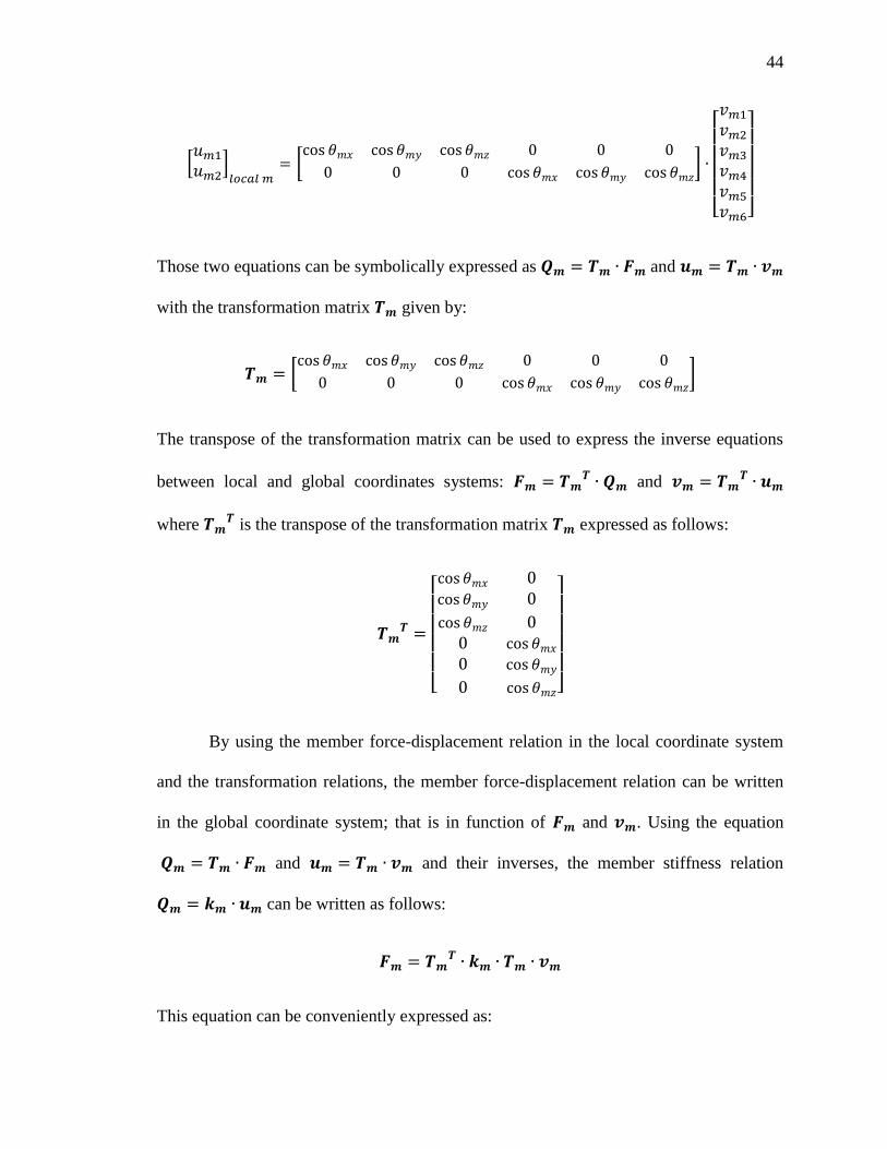
Those two equations can be symbolically expressed as and
with the transformation matrix given by:
[
]
The transpose of the transformation matrix can be used to express the inverse equations
between local and global coordinates systems: and
where is the transpose of the transformation matrix expressed as follows:
[
]
By using the member force-displacement relation in the local coordinate system
and the transformation relations, the member force-displacement relation can be written
in the global coordinate system; that is in function of and . Using the equation
and and their inverses, the member stiffness relation
can be written as follows:
This equation can be conveniently expressed as:

45
Where is called the member stiffness matrix in the global coordinate and can be
written as follows:
[
]
3.2.5 Structure stiffness relations. The next step after having determined the member
force-displacement relationship in the global coordinate system is to define the stiffness
relation for the whole structure; that is to express the external load vector as a function
of the joint displacement vector .
Hereafter, it will be shown in three steps how to relate and . For the purpose
of clarity those steps will be applied to the truss shown in Figure 3.5.

46
Figure 3.5 Displacement vector, load vector and reaction vectors
Step 1: The joint load vector is expressed in terms of the member end forces
vectors in the global system by applying the equations of equilibrium for the joints of
the structure.
{
4 4 4
6 6 6
Step 2: The joint displacement vector is expressed in function of the member
end displacements vector in the global coordinate system by using the compatibility
Z
Y
X
1
𝑑
𝑑
𝑑
𝑅
𝑅
𝑅
2
3
𝑅4
𝑅
𝑅6
𝑅7
𝑅8
𝑅9
4
𝑃 𝑃 𝑃
1
(a) (b)

47
conditions, i.e. the displacements of the member ends must be the same as the
corresponding joint displacements.
{
{
{
{
4 4 4
6 6 6
Step 3: First, the compatibility equations obtained in step 2 are substituted into the
member force-displacement relation in order to express the members’ global end forces
in function of the joint displacements. Then these forces are substituted into the joint
equilibrium equations obtained in step 1 to establish the structure stiffness relationship
between the joint loads vector and the joint displacements vector . The member
global stiffness relation for an arbitrary member m, can be written as:
[
4
6]
[ 4 6
4 6
4 6
4 4 4 44 4 46
4 6
6 6 6 64 6 66]
[
4
6]
And, using the relationships from step 2 to write the member end forces needed in the
step 1:
{
4 44 4 4 46 6
4 44 4 4 46 6
4 44 4 4 46 6
4 4 6 6
4 4 6 6
4 4 6 6
6 64 4 6 66 6
6 64 4 6 66 6
6 64 4 6 66 6

48
{
4 44 4 46
4 44 4 46
4 44 4 46
4 6
4 6
4 6
6 64 6 66
6 64 6 66
6 64 6 66
Finally using the relationships given in step 1:
{
4 4 4
6 6 6
{
( 44 44 44) ( 4 4 4 ) ( 46 46 46)
( 4 4 4) ( ) ( 6 6 6)
( 64 64 64) ( 6 6 6 ) ( 66 66 66)
These equations can be conveniently written in matrix from as:
44 44 44 4 4 4 46 46 46
4 4 4 6 6 6
64 64 64 6 6 6 66 66 66
The matrix is called the structure stiffness matrix. The dimension of the square
matrix is equal to the number of degrees of freedom. is a symmetric matrix. The
foregoing equation between the degrees of freedom and the loading is called the structure
stiffness relation and enables to calculate the structure’s displacements for any given
loading. Once the deformed shape of the structure is known, the member end forces can

49
be calculated by using the member stiffness relations. Then these member end forces are
written in their member local coordinate systems in order to find the value of the axial
forces along the individual members.
The displacement method is a straightforward method for calculating the
displacements and the forces inside a truss structure. The described procedure is easy to
implement, since it only involves solving a matrix system with parameters properly
defined from the structure’s geometry.
The structure’s stiffness coefficient of a joint in a direction equals the algebraic
sum of the member stiffness coefficient, for member ends connected to the joint. This
indicates that the structure’s stiffness matrix can be formulated directly by adding the
elements of the member stiffness matrices. This is made using numbering techniques
which enable us to assemble the structure’s stiffness matrix from the member stiffness
matrices. The figure below provides an example of numbering techniques used to
assemble the structure stiffness matrix.

50
Figure 3.6 Assembling of the structure stiffness matrix
𝑲𝟏
[ 𝐾 𝐾 𝐾 𝐾 4 𝐾 𝐾 6
𝐾 𝐾 𝐾 𝐾 4 𝐾 𝐾 6
𝐾 𝐾 𝐾 𝐾 4 𝐾 𝐾 6
𝐾 4 𝐾 4 𝐾 4 𝐾 44 𝐾 4 𝐾 46
𝐾 𝐾 𝐾 𝐾 4 𝐾 𝐾 6
𝐾 6 𝐾 6 𝐾 6 𝐾 64 𝐾 6 𝐾 66]
𝑲𝟐
[ 𝐾 𝐾 𝐾 𝐾 4 𝐾 𝐾 6
𝐾 𝐾 𝐾 𝐾 4 𝐾 𝐾 6
𝐾 𝐾 𝐾 𝐾 4 𝐾 𝐾 6
𝐾 4 𝐾 4 𝐾 4 𝐾 44 𝐾 4 𝐾 46
𝐾 𝐾 𝐾 𝐾 4 𝐾 𝐾 6
𝐾 6 𝐾 6 𝐾 6 𝐾 64 𝐾 6 𝐾 66]
𝑲𝟑
[ 𝐾 𝐾 𝐾 𝐾 4 𝐾 𝐾 6
𝐾 𝐾 𝐾 𝐾 4 𝐾 𝐾 6
𝐾 𝐾 𝐾 𝐾 4 𝐾 𝐾 6
𝐾 4 𝐾 4 𝐾 4 𝐾 44 𝐾 4 𝐾 46
𝐾 𝐾 𝐾 𝐾 4 𝐾 𝐾 6
𝐾 6 𝐾 6 𝐾 6 𝐾 64 𝐾 6 𝐾 66]
𝑺 𝐾 44 𝐾 44 𝐾 44 𝐾 4 𝐾 4 𝐾 4 𝐾 46 𝐾 46 𝐾 46
𝐾 4 𝐾 4 𝐾 4 𝐾 𝐾 𝐾 𝐾 6 𝐾 6 𝐾 6
𝐾 64 𝐾 64 𝐾 64 𝐾 6 𝐾 6 𝐾 6 𝐾 66 𝐾 66 𝐾 66
𝑥 𝑦 𝑧 𝑥 𝑦 𝑧 𝑥 𝑦 𝑧 𝑥 𝑦 𝑧
𝑥 𝑦 𝑧 𝑥 𝑦 𝑧
𝑥 𝑦 𝑧 𝑥 𝑦 𝑧
𝑥 𝑦 𝑧 𝑥 𝑦 𝑧
𝑥 𝑦 𝑧 𝑥 𝑦 𝑧
𝑥 𝑦 𝑧
𝑥 𝑦 𝑧

51
3.3 Classical method to compute the probability of failure of a structure using
failure paths
3.3.1 Framework. In the reliability analysis of a structural system, the probability of
no structural failure under the applied loads is investigated. To do so, one should specify
the probability of the failure of the structure’s members and those of the failure paths.
The development of system failure paths requires structural analysis of the intact
structure to determine the forces within the truss system. Given this force distribution, a
probabilistic analysis using the loads and the member resistances as random variables is
conducted to compute the probability of failure for every single member.
In practice, real structures can have numerous members; and thus it is not possible
to enumerate and compute a probabilistic analysis for all of them. In these cases, some
studies have shown that the structural reliability, i.e. the probability of no failure, can be
estimated efficiently by using only dominant failure members. However, in this presented
method, all the members are considered as candidate to failure; this leads to a complete
enumeration of all the failure paths.
Then, to perform the next step which is to compute a member probabilistic
analysis for the damaged structure, subsequent structural analyses are required. To do so,
a post-failure behavior must be specified for the failed member. Usually, two different
idealized behaviors are chosen to describe the constitutive law within the failed member.
The first behavior is the brittle failure which considers that a failed component does not
yield and cannot carry any additional load. In this case, the component is removed from
the truss geometry in the structural analysis. The second failure is the ductile failure
which in the case of an idealized perfectly plastic material considers that the member
cannot carry any additional load but can accommodate infinite displacements. In this
52
case, the component is removed from the truss geometry and replaced by a load equal to
the force carried by the failed member corresponding to yielding. In this presented
method, the fracture is conservatively and consistently set as a brittle failure.
Structural analysis and probabilistic analysis are alternately computed following
the process described above until the formation of a failure mechanism in the structure,
i.e. the structure has become unstable. Such a mechanism occurs when the structure’s
stiffness matrix becomes singular and has its determinant equals to zero. Thus the given
failure path has reached to it end.
When all the failure paths have been found and the reliability analysis at the
member level has been computed for all members in all scenarios, the structure’s
reliability is computed. Further discussions on the structure reliability evaluation from the
member reliability will be provided later in this chapter.
To picture the variety of the failure paths, different diagrams can be used. One
such diagram was described in chapter 2 (i.e., the failure path diagram). Another one is
an analogy with series and parallel systems to depict the possible failures of the structure.
In a statically indeterminate truss, the member failures are considered as parallel failures
since only if all the member of a given failure path occur, the structure will fail. On the
other hand, when considering the occurrence failure paths leading to the failure of the
structure, failure paths are said to be in series.

53
Figure 3.7 Parallel and series systems
3.3.2 Component reliability. In structural codes, design equations are written at the
member level which is considered as the controlling element. To do so, effects of
structural parameters such as loading, geometry and materials must be expressed at the
member level; and structural theories must be developed to fulfill this purpose. Thus,
most of the structural knowledge delivered by the codes is related to the member. The
reliability analysis aims to be a global analysis of the structure; however, to benefit from
most of the state of knowledge in structural engineering, the reliability analysis must
comply with design requirements and be performed, at least for a primary approach, at
the component level.
A structural component is subject to forces which, if exceeding a given level
called member resistance, will cause its failure. Several modes of failure such as tensile
failure, compressive failure, shear failure, stability failure, fatigue failure can occurs for
the same member. These potential failure modes can be written as a limit state in terms of
the member resistance and the load effect on the considered member . Each limit
states must be considered in evaluating the probability of failure of the component. Thus,
Member 1
Member 2
Member 3
Member 2
Member 4
Member 5
Member 6
Member 2
Member 1
Member 3 Failure path 1
Failure path 2 Failure path 3
Failure path 4

54
the probability of failure of a component with potential failure modes can be written
as follows:
(
)
Where:
represents the event of failure for the component in its mode of failure .
Because of the correlation between modes of failure the component probability of
failure cannot be calculated using this formulation. Given some mathematical conditions
concerning the events of failure, it can be shown that the component probability of failure
is bounded by two extreme situations. If all the failure modes are perfectly correlated:
( (
) ( ) (
))
And if all the failure modes are statistically independent:
∏( (
))
<
These two cases could be chosen as two bounds for the actual . Indeed, in
reality the failure modes are neither perfectly correlated nor statistically independent.
However, in the case of the failure of a single member, the failure modes written in terms
of limit states are highly correlated because the same random are used to write the
resistance and the load effect for the different modes of failure. Thus, the case of
perfectly correlated modes of failure can be taken as an acceptable approximation of the

55
member probability of failure. In this study, an additional approximation is considered.
This is in assuming that the controlling mode of failure is either the tensile or
compressive mode. A member is said to have failed when it has started yielding. This
approximation is made to simplify the analysis and is exact in most cases. The yielding
mode of failure can be written in term of and as follows:
Where is the variable representing the member resistance whereas is the
variable corresponding to the load effects on the considered member. The variables and
are defined by using a set of variables representing the loading and the structure
geometry and materials. The component is considered to have yielded when is less
than . The equality between the two variables defines the limit state. A performance
function can be introduced as:
The limit state is defined by the zeros of the performance function and the
member is considered to be failed when is negative. Assuming statistical independence
between and , which is close to the reality given that and are not written with the
same variables and considering that these basic random are statistically independent, the
following properties can be established for the performance function .
( ) ( ) ( )
( ) √ ( ) ( )

56
Where:
( ) ( ) and ( ) are respectively the expected value the performance
function, the resistance and the load effect the considered member.
( ), ( ) and ( ) are respectively the standard deviation of the performance
function, the resistance and the load effect on the considered member.
Further calculations require assigning a distribution function to the performance
function variable. The normal distribution function is chosen as a realistic and simple
candidate.
( ( ) ( ) )
Using the linear transformation below, it can be shown that:
( )
( ) ( )
Where is the symbol used to refer to a normal distribution function. The
parameters of the normal distribution of are the expected value and the variance ( ) .
( ) is the standard normal distribution, i.e. a normal distribution with zero as an
expected value and a variance equals to one.
Using the performance function to represent the failure, the failure probability is
given as follow:
( ) ( ( ) ( ) )( )

57
Where ( ( ) ( ) ) is the cumulative distribution function of the normal
distribution function assigned to the performance function . Using the linear
transformation showed above:
( ) (
( )
( )) ( ) (
( ( ) ( ))
√ ( ) ( ) )
The probability failure of the member is defined in terms of its resistance and
load effect expected value and standard deviation.
The inverse of the probability of failure is the probability of survival which is the
reliability of the member and is written as follows:

58
(a) Standard normal distribution
(b) Normal distribution of
Figure 3.8 Member probability of failure associated with Z
0
0.1
0.2
0.3
0.4
0.5
-5 -4 -3 -2 -1 0 1 2 3 4 5
0
0.04
0.08
0.12
0.16
-10.5 -7.5 -4.5 -1.5 1.5 4.5 7.5 10.5 13.5 16.5 19.5
𝑃𝑓𝑐𝑖
𝑃𝑓𝑐𝑖
𝜎(𝑍)
𝔼(𝑍) 𝑍
φ(𝔼(𝑍) 𝜎(𝑍) )(𝑍)
𝑍 𝔼(𝑍)
𝜎(𝑍)
φ( ) (𝑍 𝔼(𝑍)
𝜎(𝑍))

59
3.3.3 Structure’s reliability. In an indeterminate structure, the failure of a component
does not necessarily leads to the failure of the structure. In fact, the failure is cause by a
succession of failures among structural members, which is called a failure path.
Numerous failure paths can exist within a structure. To compute the probability of failure
of the structure, one should be able, first, to quantify the probability of occurrence of all
single failure paths and, then, to prescribe a method to evaluate the probability of failure
of the structure from those of its failure paths.
Owing to the above proposed framework, the reliability of every member in all
possible scenarios can be computed. These member-related data are the only available
data to compute the structure’s reliability.
First, the probability of occurrence of a failure path must be computed. This
requires the calculation of the probability of multiple events using the conditional
probability. The probability of the occurrence of the failure mechanism (starting by the
failure of the member 1 and ending with the failure of member n, can be written as
follows:
Where is the probability of failure of the first component in the failure path
for the intact structure, is the probability of failure of the second component given
that the first component has failed and is the probability of failure of the
last component of the failure path given that the other component has failed first. These
probabilities are evaluated using the member reliability for all scenarios considered in the
structural analysis framework.

60
Then the probability of failure of the structure is evaluated from those of its
failure paths. A structural system with k failure paths will have a probability of failure
written as:
( )
Where correspond to the occurrence of the failure path denoted by . As it was
shown for the different modes of failure of a single member, the evaluation of the
probability of failure of the structure is impractical because of the correlation between
failure paths. It was also shown that such a probability can be bounded as follows:
( ( ) ( ) ( ) ∏( ( ))
<
In some studies, affirming that the two bounds are close, it was permitted to approximate
with the two bounds average:
( ( ) ( ) ( ) ∏ ( ( ))
<
The probability of survival of the structure is written in function of the probability of
failure as follows:

61
3.3.4 Shortcomings of the proposed method. The main objective of this chapter was
to provide the reader a comprehensive approach to a classical method to compute the
probability of failure of a structure. Thus, the reader was made aware of the assumptions
made, the reliability and structural theories used were introduced and the global
framework leading to the computation of the structure probability of failure was
explained. This method is said to be classical because most of the introduced hypotheses
are those used in the structural reliability literature. However, this method, besides
providing a comprehensive approach, has several shortcomings as explained below.
3.3.4.1 The method is time consuming. In case of a real structure, due to the number of
members, numerous failure paths are to be computed. At every stage of every failure path
a structural analysis and a reliability analysis must be done. In practice the time needed
by a computer to provide the structure’s probability of failure following this method
increases drastically with the number of components and become impractical for real
structure. It was demonstrated in [13] that a good approximation of the probability failure
can be given using automatic generated stochastically dominant failure paths. This results
in less effort in conducting structural and reliability analysis. It was also shown that the
structural analyses can be done more efficiently using the force method instead of the
displacement method [7]. In [7] the authors present an improved force method which is
easy to implement and reduces the number of calculations to conduct a structural
analysis. Among all those efforts to reduce computational time, most of the methods take
advantage of the fact that identical structural and reliability analyses are needed to be
considered. Every stage of a failure path corresponds to a different scenario; however, if
the order of member failure is ignored, scenarios were the same members are involved in

62
the failure path can be considered as being identical. This can be done without
influencing the final probability of failure because the structural and reliability analyses
do not take into account the order in which members have failed. Thus ignoring the
sequence of component failure can lead to faster computations.
3.3.4.2 Significance of correlation among member failures and paths. The classical
methods are incapable of dealing with the correlation in member failure and in failure
paths. Concerning the member failure, it is assumed individual member conditions are
independent; and as such, the reliability analysis can be conducted for members as stand-
alone structural components. However, it is obvious that because of the common loads
and the fact that materials are often obtained from the same source, conditions among
members may be partially correlated. When a reliability analysis is conducted on a single
member, these load effect and properties correlations have no direct effect in the results,
since the conditions among members are considered independent. However, looking
globally at the structure, the event of failure of a member shares many common
parameters with other members. This indicates that at least in some members, once one
failed, they others have also failed. For example, consider two members sharing the same
properties. Let’s further assume that for every given load, member 1 is taking more load
effect that member 2. Thus member 1 is more vulnerable to failure; and its failure
probability will be evaluated according to its internal load and its resistance. However,
member 2 will never fail in this particular scenario, since member 1 will need to fail first.
The probability of failure of the member 2 is therefore zero, if member 1 has not failed
yet. It is obvious that in reality this cannot be possible.

63
In the case of failure paths, it was recognized that they may be correlated. However, for
simplicity, again, all failure paths were assumed to be independent. The two bounds thus
obtained for the system failure probability correspond to the two extreme situations
where either all the failure paths are totally correlated or they are totally independent.
Madsen and Ditlevsen [2] elaborate further on this shortcoming and offer solutions to
have more accurate bounds for the system failure probability. Moreover, it should be
noticed that in the case of totally correlated failure paths, the corresponding bound is
inconsistent with actual conditions, since in reality the paths are almost never perfectly
correlated.
3.3.4.3 The load issue. In classical methods, in any scenarios, when the reliability
analyses are computed in terms of the load effect and the member resistance , the
characteristics of the random variables needed to compute and remain the same
throughout the loading regime. These characteristics will need to be updated as the
loading regime continues and the nature and number of failure mechanisms keep on
changing. Using classical methods, a member failure will affect the structure geometry
but not the random variables representing the member properties and the loading. This is
an over-simplification. To clarify this shortcoming, consider the following example.
Two successive member failures are considered. Due to an unexpectedly high
load, member 1 fails. Using the classical methods, one uses the estimates of the load and
resistance and computes the probability of failure for member 1.. Now assume that this
unexpectedly high load no longer applies on the structure. A redistribution of the loads
occurs within the structure and thus a second reliability analysis can be conducted to
evaluate the probability of failure of member 2. We realize that using this process, the

64
unexpected high load (which affected member 1) will not damage the structure beyond
member 1. However, the method will treat the system as though the unexpected high
load is persistently applying on the structure.
In a realistic situation, a failure happens because of the simultaneous occurrences
of an unexpectedly high load and weak member resistance. If the load causes the failure
of a member (the first member failed) and starts a failure mechanism, there are chances
that it will damage consecutively several other members. When reliability analyses are
conducted separately, as it is the case in classical methods, the random variables
governing the loading must be updated every time a new reliability analysis is conducted
on the structure. In the same manner, because member properties are partially correlated
among each other, the knowledge of upon a member failure, the random variable
describing the properties of surviving members will need to be updated.
Among assumptions and simplifications made in classical methods, the one on constant
load is perhaps affecting the final results for the probability of failure most. This is
because; this assumption minimizes the effect of a strong load that may only
unexpectedly apply on the structure, and missed when conducted the reliability analysis.
3.3.4.4 The issue related to the member post failure behavior. In this method, a failed
member is a member which has started yielding. Once a member is said to be failed, it is
considered as absent in the structure. Considering that a yielded member cannot carry any
load is far from being true. In reality, when a member is yielding it can still at least carry
the same load. In that model, the material redundancy is not considered at all. As it was
mentioned earlier, the material redundancy corresponds to the additional load and
additional displacement that a member can withstand after having yield. The material

65
redundancy which corresponds to additional load is called the constraint redundancy and
the redundancy which corresponds to additional displacement is called the displacement
redundancy.
Experimentations are conducted on materials to plot the stress-strain constitutive
relation of the considered material. For common materials, the shape of the stress-strain
curve is well-know and mathematical model are formulated in order to use the material in
structural analysis. Two simple models which take into account the material redundancy
consider the material as:
Linear elastic – perfectly plastic. An example of a stress-strain curve of such a
material behavior is given by the figure 2.5 (b).
Linear elastic – linear work hardening plastic. An example of a stress-strain curve
of such a material behavior is given by the figure 2.5 (d).
Contrary to the classical method, these two descriptions of the material behavior
are a good approximation of the real material behavior. In the research literature,
numerous examples of reliability methods using the linear elastic – perfectly plastic
approximation can be found. Indeed, this approximated behavior can be easily
implemented in the structural analysis. When a member is considered as failed, instead of
just removing it from the structure geometry as it is done in the classical method, two
equal forces corresponding to the yielding strength of the member are added to the
structural model as additional loads. These additional loads are located at the two pins
where the failed member was attached before and act in the failed member direction.

66
3.3.4.5 The issue related to the member mode of failure. In this method, the mode of
failure is selected. Probabilities are not computed at a member level in order to know
which mode failure is dominant and what is the final probability of failure of the member
given that all possible modes of failure are considered. Considering multiple mode of
failure in a member would lead, because of the partial correlation between modes of
failure, to the need of the computation of bounds.
3.3.5 Concluding remarks. Globally, the features to improve in this classical method
of computing the probability of failure of a structure can be gathered in three main
aspects which are
The computational time of the method. Failure paths are numerous and analyses
required are time consuming. The main issues regarding with this aspect are the
number of scenarios to be considered and the computer time needed to compute
all the structural analyses.
The realistic representation of the failure mechanism. The framework in which
analyses are conducted must compel to the reality of the structure failure
mechanism. The main issues regarding with this aspect are the misrepresentation
of the loading, the correlation between member failure and the post failure
behavior of a member.
The approximation made within the method. They must be precise and use as
many information as possible. The main issue regarding this aspect is the bounds
given for correlated failure path.
67
CHAPTER 4
MODIFIED METHOD FOR COMPUTING THE PROBABILITY
OF FAILURE OF A STRUCTURE
4.1 Introductory remarks
The purpose of this chapter is to propose a modified method to compute the
probability of failure of a structure based on the classical framework introduced in
chapter 3. The method is based on revised hypotheses and new strategies to compute the
reliability and structural analyses are introduced. The main objective is to provide an
improved method with regards to the shortcomings of the classical methods. However,
for the sake of simplicity, these modifications do not affect the classical method
framework. This improved method uses materials taken from Ditlevsen and Madsen [2].
4.2 The limit state model
4.2.1 Limit state. A failure limit state is a load requirement beyond which a structure is
said to be failed. This requirement is formulated with a mathematical model which
usually includes, as input variables, the structure’s geometry and mechanical properties
as well as the applied loads. A scalar function is used to define a limit state as follow:
* ( ) +
Where,
is a scalar function defining the limit state
is the vector describing the structure and its load
is a subset of

68
The components of the vector are the independent variables that describe the
structure’s geometry, the structure mechanical properties and the applied loads. These
variables are considered free in the sense that their values can be chosen freely and
independently in the subset of . The subset is the domain of definition of the
model. Every choice of in corresponds to a uniquely-defined structure and its applied
loads. Thus, is a pure mathematical expression, which may not be physically possible.
For example, when the loads exceed the capacity of the structure, the failure occurs; so
physically the notion of load being larger than the resistance is no longer valid. The limit
state defines two sets within, which are defined as follows:
Safe set:
* ( ) +
In the safe set, the requirement defined by the limit state is said to be satisfied.
Failure set:
{ ( ) }
In the safe set, the requirement defined by the limit state is not satisfied.
The boundary of the safe set, which is the boundary of the boundary of the failure
set also, is the limit state.

69
Figure 4.1 Von-Mises Criterion limit state
Figure 4.1 depicts the Von-Mises limit state, which is defined via the stress
components 1 and 2, as well as the yield stress y. The safe set and the failure set are a
partition of . This property is a consequence of the definition of on Thereafter, for
the sake of simplicity; the limit state will be represented by the zeros of the scalar
function, that is . For later use, the scalar function will be required to be piecewise
differentiable on . Moreover, the limit state scalar function will take positive values in
the internal of the safe set and negative values in the internal of the failure set. It should
be noted that the choice of is not unique: the same limit state can be defined with a
different scalar function.
Mainly, limit states can be of two different categories which are the failure limit
state and the serviceability limit states. The first category represents a situation where the
structure is about to lose its integrity. The structure will be at least damaged and the
𝝈𝟐
𝝈𝟏 Safe set
Limit set
Failure set

70
initial situation cannot be recovered. The second category corresponds to the limit
situation where the structure is about to not be able to fulfill the requirement for which it
was designed. This second situation is necessary in design; but since it is reversible it
does not raise any reliability issues. In the hereafter, only failure limit state will be
considered.
4.2.2 Linear limit state. A linear limit state is defined by a linear scalar function ,
(also called linear form), as follows:
* ( ) +
Where,
is the linear form defining the limit state. is written as follows:
( )
are given constant coming from a structural analysis and a
definition of the limit state.
are the variables of the model.
The limit state defined an n-1 dimensional hyperplane which separates the domain
of definition of the model in two sets: the safe set and the failure set.
Remark: The safe set is a convex set, which means that if and belong to the
safe set, for every in the interval , -, ( ) is in the safe set. Owing to this
property, convex sets, defined by a form linear or not, are particularly convenient for
limit state analysis [2]. Moreover, any limit state having a convex safe set can be
described as the intersection, finite or infinite, of linear limit states. Finally, it should be

71
noted that in the case of linear limit, even the failure set is convex. The case of non-
convex failure set is demonstrated in Figs. 4.3 and 4.4.
Figure 4.2 Linear limit state
Figure 4.3 Non-convex safe set
Safe set
Failure set
Limit state
𝑥
𝑥
Safe set
Failure set
Limit state
𝒙𝟏
𝒙𝟐

72
Figure 4.4 Non-convex failure set for a concrete column.
Hereafter the possibility to describe a convex set as an intersection of linear limit
state will be used to approximate a non-liner limit state by a given number of linear limit
states.
4.2.3 Multiple linear limit states. In practice, a structure has multiple modes of failure,
which must be taken into account by the definition of multiple failure limit states (figure
4.5 and 4.6). These modes of failure stem, for instance, from the failure of different
elements within the structure or from the different possible failure modes in a member,
such as shear or bending moment modes of failure. Considering these modes of failure
will lead to a larger domain of definition of the structure and load variables, since more
variables will be needed to describe the model. In this domain, every mode of failure has
a corresponding limit state function, which is a linear form in the case of linear limit
state. The new safe set is the intersection of all the safe set corresponding to different
single modes of failure.
Safe set
Failure set Limit state
𝑴𝒖
𝑷𝒖

73
For limit state with regard to the mode of failure :
* ( ) +
In which,
is the linear forms corresponding to the limit state
( )
Safe set when the limit state is taken as a single limit state:
* ( ) +
Safe set for a multiple linear limit state:
* ( ) + ⋂* ( ) +
The safe set for a multiple linear state is defined as the intersection of every single safe
set.
Figure 4.5 Multiple linear limit state in 2-dimensional space
Safe set
Failure set Limit state 1
𝒙𝟏
𝒙𝟐
Limit state 2

74
Figure 4.6 Multiple linear limit states in 3-dimensional space
4.3 Probability calculations for linear limit state
The limit state model described above is enough to design safe structures for
deterministic variables, because in this model the variables describing the structure and
its loads are either in the safe set or in the failure set. However, because of the
randomness in design parameters, a model incorporating random variables is needed in
order to measure the structure safety. In the probabilistic model, introduced next, the
probability of to be on the safe set will be defined as a measure of the safety or
reliability of the structure. The part 4.3 of this study is taken from [2].
Safe set
Limit state 2
Limit state 1
Failure set
𝒙𝟏
𝒙𝟐
𝒙𝟑
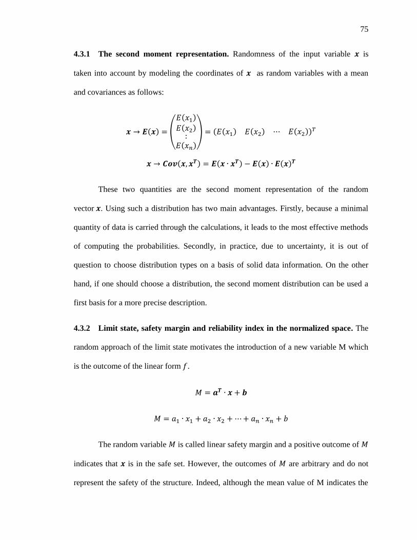
75
4.3.1 The second moment representation. Randomness of the input variable is
taken into account by modeling the coordinates of as random variables with a mean
and covariances as follows:
( ) (
( )
( )
( )
, ( ( ) ( ) ( ))
( ) ( ) ( ) ( )
These two quantities are the second moment representation of the random
vector . Using such a distribution has two main advantages. Firstly, because a minimal
quantity of data is carried through the calculations, it leads to the most effective methods
of computing the probabilities. Secondly, in practice, due to uncertainty, it is out of
question to choose distribution types on a basis of solid data information. On the other
hand, if one should choose a distribution, the second moment distribution can be used a
first basis for a more precise description.
4.3.2 Limit state, safety margin and reliability index in the normalized space. The
random approach of the limit state motivates the introduction of a new variable M which
is the outcome of the linear form .
The random variable is called linear safety margin and a positive outcome of
indicates that is in the safe set. However, the outcomes of are arbitrary and do not
represent the safety of the structure. Indeed, although the mean value of M indicates the

76
mean distance from to the limit state in , this distance has nothing to do with
probabilities and does not enable to compare different limit states. To illustrate the fact
that the outcomes of are arbitrary, it should be recalled that the same limit state can be
written in terms of different linear forms. In the case of linear forms, these different linear
forms can be found after multiplication of a first linear form by an arbitrary constant.
Thus, one of the purposes of this chapter is the establishment of an invariant number
capable of comparing safety margin with regards to overpassing the limit state.
The objective is to interpret the mean distance from to the limit state in , i.e.
( ), as a consistent measure of safety. To do so, the standard deviation of is taken
as a unit, and the reliability index is introduced as follows:
( )
( )
( )
√ ( )
This number is unchanged after a multiplication of the linear form defining the
linear limit state. That means that all linear forms representing the same limit state are
assigned with the same reliability index. Moreover, it can be shown that the number is
invariant under any regular inhomogeneous linear mapping of the random into another
random vector . [2]
( )
Under a specific linear mapping of the vector a new vector can be defined
with the following properties:

77
( )
( )
In this particular mapping space has the following convenient expression:
( )
( )
( )
√ ( )
√
This final expression of the reliability index is convenient because it is also the
distance from the origin to the hyperplane defined by the linear limit state in the specific
mapped space just defined above. Hereafter, this space will be called the normalized
space (figure 4.7).
Figure 4.7 Geometric interpretation of the reliability index in the normalized space
𝒚𝟏
𝒚𝟐
Limit state
Safe set
Failure set
𝒏
𝒙𝟏
𝒙𝟐
𝜷
1
1
1 1 E(x)

78
The invariant number can be interpreted as a measure of safety with respect to
overpassing the limit state. According to its definition it measures the distance from the
limit state represented by to the mean value ( ) with the standard deviation
( ) taken as a unit. The parameter enables to have an insight regarding safety of the
structure with respect to the reliability; however it does not give a measure of the
probability of overpassing the limit state. To do so, additional information concerning the
input random variables, such as distribution functions must be provided.
4.3.3 Distribution function. The model described above includes a limit state and a
random variable described by its second moment and defines a comparison criterion
among limit states by using the reliability index. This criterion can be considered as a
reasonable engineering reliability comparison, since it is enough to define a structure’s
safety condition with respects to reliability. However it is impossible to compute the
probability of failure using only the safety index.
To compute probabilities, distribution functions must be assigned to the initial
input random variables. For simplicity, the input random variables are assumed to
follow a normal density function. Thus, the random vector follows a multivariate
normal distribution of dimension with the -dimensional mean vector and the
covariance matrix.
( ( ) ( ) )
. ( ) ( )/
( ) √ ( )
(; ( ; ( ))
( )
( ; ( )))

79
This multivariate normal density function can be transformed into a standard
normal multivariate density function. This conveniently enables us to conclude that
follows a standard normal multivariate density function.
( ( ) ( ) ) ( )
( ) (
√ *
.; / ( ) (
√ *
; (
: : :
)
In the normalized space, the components of are independent and have a
variance equals to 1 with an expected value of 0.
The density of is constant on every hypersphere centered at the origin of the
normalized space. This is consistent with the reliability index which depends only on the
distance between the considered hyperplane and the origin. This property which is called
the rotation symmetry reflects a reasonable engineering comparison between limit states
and is consistent with the second moment representation [2].
The distribution function for a given distance between the origin of the
normalized space and the end of the vector is calculated as follows:
(‖ ‖ ) ∮ (
√ *
; (
: : :
)
This integration can be performed by recognizing a similarity with the
distribution. Indeed, the distribution corresponds to the distribution of the sum of the
square of random variable following a standard normal distribution.
‖ ‖ ( )

80
‖ ‖ (√ √ )
The distribution function for a given distance from the origin of the normalized
space is the distribution with degrees of freedom, a mean value equals to √ and a
variance equals to √ .
4.3.4 Probability of failure of a single linear limit state. It has been seen that the
reliability index defines the level of safety of a linear limit state. The addition to a
distribution function to the input variable enables to evaluate the distribution function
for and for any distance from the origin in the normalized space. Thus, the probability
of being in the failure set could be evaluated by an integration of the density function of
on the failure set as follows:
( ( ) ) ∫ . ( ) ( )/
( ( ) ) ∫
( ) √ ( )
(; ( ; ( ))
( )
( ; ( )))
( ( ) ) ∫ ( )
( ( ) ) ∫ (
√ *
; (
: : :
)
The result of these integrals would be the exact probability of failure given a
linear limit state. Although, the calculation of this integral is not really complicated, it has

81
never used in the literature, as an approximation of the probability of failure based on the
reliability index is preferred.
According to its definition, the safety index measures the distance from the limit
state represented by to the mean value ( ) with the standard deviation ( )
taken as a unit. Assuming that the safety margin follows a normal
distribution, ; ( )
( ) follows a standard normal distribution. The probability of can
be computed using as follows (see Figure 4.8):

82
(a) Assumed distribution function for the safety margin
(b) Reliability index
Figure 4.8 Reliability index and safety margin distribution
0
0.04
0.08
0.12
0.16
-10.5 -7.5 -4.5 -1.5 1.5 4.5 7.5 10.5 13.5 16.5 19.5
0
0.1
0.2
0.3
0.4
0.5
-5 -4 -3 -2 -1 0 1 2 3 4 5
φ(𝔼(𝑀) 𝐷(𝑀) )(𝑍)
𝜎(𝑍)
𝔼(𝑀) 𝑀
φ( ) (𝑀 𝔼(𝑀)
𝐷(𝑀))
𝑀 𝔼(𝑀)
𝐷(𝑍) 𝛽

83
Thus, the probability of failure is:
( ( ) ) ( ) ( )
In which:
is the standard normal cumulative distribution function.
In the case of the probability of survival, the outcome of the safety margin is in
the safe set, that is ( ) . Thus, the probability of survival is:
( ( ) ) ( )
4.4 The load continuity hypothesis
Before, introducing the load continuity hypothesis, the context in which it takes
place must be explained. As explained later, the limit state governing a member failure
can be approximated as linear limit state. In this approximation, the input variables
representing the structure geometry and materials are considered as constant and only
input variables which are considered to be random are the loads. In this approximation
the vector describes solely the loading.
4.4.1 Introduction of a loading evolution function. In the development of the limit
state theory, independent variables are chosen to describe the structure and its loading.
The purpose of these variables is to form a mathematical object on which limit states
equation can be formulated. However, this object is purely mathematical and may in
some case represent an impossible situation. A simple example can be given as the model
describing a loading that is larger than the carrying capacity of the structure.

84
As reported in the literature, when randomness is associated to the input variables,
the occurrence of the impossible situation corresponding to the input vector in the
failure set is taken as the occurrence of failure. Indeed, it was explained, that the
probability of failure with regard to a limit state is the probability of the safety margin to
be negative, which is the probability of the input vector to overpass the limit state
which correspond to a physically impossible situation.
Furthermore, limit states are approximated to linear limit state by considering
only the loads as random variables. Given this description, an impossible situation is the
occurrence of a loading which has overpassed the limit state. This situation is physically
impossible because the physical nature of loads does not enable them to be suddenly
equal to a given value. The evolution of the loading in time is continuous. This motivates
the introduction of a loading evolution function which represents for any time the value
of the loading. This parametric function is continuous on its domain.
At the first glance, the definition of a loading evolution function may appear
contrary to the definition of random loading, which basically considers that any load can
suddenly occur with an associated probability of occurrence. These two concepts are
compatible; however, for any possible outcome of the random loading, the loading
evolution function can be plotted from the origin of the space to the desired outcome.
Thus, the final loading, which is the loading given by the loading evolution function for
its largest application time, corresponds to the outcome of the random loading (see Fig.
4.9).

85
Figure 4.9 Loading evolution function in the subset
As sown in Fig. 4.9, the evolution function ( ) can be with the following properties:
( ) is continuous
( )
Moreover, it is seen that for any in the failure set, the physical failure with
respect to the limit state has occurred. Thus, the probability of having in the failure set,
although being an imaginary situation, corresponds to the probability of failure.
( ( ) ) ( ( ( )) )
Where:
( ( ) ) is calculated using the linear state theory described above.
Safe set
Failure set
Limit state
𝑥
𝑥
𝒙(𝒕)
𝒙
Physical failure

86
( ) is the load evolution function
( ( ( )) ) is a definition of the probability of failure consistent with
the load continuity.
This description of the continuity of the loading will be more significant in the
case of multiple linear limit state and when it will be needed to ensure the continuity of
the load in order to compute a second failure in the structure.
4.4.2 Elimination of inconsistent limit states. In the case of a multiple limit space, it
is possible that, for a given outcome of the input variable vector , the load evolution
function crosses to limit state hyperplanes. This case corresponds to no physical reality,
since overpassing one limit state induces the failure of the structure. However, if this
situation is implemented without modification in a reliability model, a probability may be
assigned to the occurrence of being in the failure set which is completely included in
another failure set. Figure 4.10 depicts a situation where multiple limit states are
considered. The failure set corresponding to some of them can only be reached if the load
evolution function has crossed another limit state hyperplane first. In order to make the
reliability model more consistent with the reality, these particular limit states should be
removed from the model. Figure 4.11 shows the reliability model which should be
considered for this case.
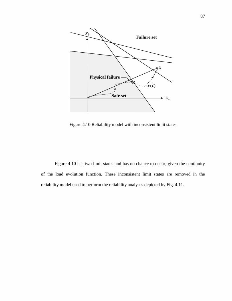
87
Figure 4.10 Reliability model with inconsistent limit states
Figure 4.10 has two limit states and has no chance to occur, given the continuity
of the load evolution function. These inconsistent limit states are removed in the
reliability model used to perform the reliability analyses depicted by Fig. 4.11.
Safe set
Failure set
𝑥
𝑥
𝒙(𝒕)
𝒙
Physical failure

88
Figure 4.11 Corrected reliability model without inconsistent limit states
4.4.3 Elimination of unnecessary limit states. In order to accelerate the reliability
analyses, a criterion to eliminate any unnecessary limit state can be established. The
probability associated with the failure set of an unnecessary limit state is very low and
can be neglected. To do so, a criterion must be defined to detect unnecessary limit states.
This criterion is arbitrary. For example, using the reliability indices calculated with the
single linear limit state theory, a criterion for unnecessary limit states could be to have a
reliability index larger than a number of times the smallest reliability index calculated.
Thus, if is the reliability index associated with the limit state , this limit state is
considered as unnecessary if ( ).
Safe set
Failure set
𝑥
𝑥

89
Figure 4.12 Reliability model with unnecessary limit states
Figure 4.12 has one limit state whose reliability index is larger than the smallest
reliability index times a given coefficient . This limit state corresponds to very few
probabilities and can be neglected in order to speed up the reliabilities analyses. Figure
4.13 shows a corrected reliability model after removal of unnecessary limit states.
Safe set
Failure set
𝑥
𝑥
𝜷𝟏
𝜶 𝜷𝟏
𝜷𝟐
𝜷𝟑

90
Figure 4.13 Corrected reliability model upon removing unnecessary limit states
4.4.4 The post failure continuity of the load. As previously explained in this chapter,
the load continuity function is introduced to take into account the continuity of the load.
This function is continuous at any given time and has no reason to be discontinuous when
a failure occurs in the structure. Indeed, in reality, the loading of a structure does not
depend of the behavior of the structure. However, in the classical methods presented
earlier, the failure of a member occurs by an outcome of the random loading vector in
the failure set. This given outcome is not considered as a candidate for the failure of a
second member, since it is not considered any longer once a first failure has occurred.
Thus another outcome of the random vector in the new failure set is required to cause
the failure of a second member. This process forces the function representing the load
evolution to be discontinuous when a failure occurs within the structure, which is not a
Safe set
Failure set
𝑥
𝑥

91
realistic description of the reality and does not agree with the load continuity hypothesis.
Moreover, since the random characteristics of the random load vector are not updated
after a failure, the expected value of the next outcome of , to be computed after a
failure, is the expected value of the initial vector which is often, conservatively, located
far from the failure set. Thus, the transition between an outcome in the failure set and the
next outcome to be computed is not continuous and gives additional chances of survival
to the structure with regard to a second failure.
In reality, the load has no reason to change instantly because of a failure and the
outcome of the vector should be considered as a candidate for multiple failures.
However, this cannot be done since the probabilistic theories introduced before do not
enable us to know the outcome of , which has caused the failure. Nevertheless, the
distribution function for is known and the most probable outcome given a particular
failure can be computed. Thus, as an approximation of the loading continuity, the
variable which should be used to check if any more failures occur within the structure
should be the most probable outcome given the occurrence of a particular failure. With
consistency with the random variable , and by recognizing that the actual outcome of
may be different than the most probable outcome of given the occurrence of a
particular failure, a new random variable should be introduced. This random variable
will have an expected value equal to the most probable outcome of given the
occurrence of a particular failure. Furthermore, its variance equals the residual variance
between and the most probable outcome of , which is the variance of the distance
between and the most probable outcome of Thus the random variable is updated to

92
compute a second failure; and a new second moment description is assigned to when a
failure has occurred.
( ( ) ) (
( ( ) )
( ( ) )
( ( ) )
,
(( ( ( ) )) ( ( ( ) )) )
4.5 The most central failure point
4.5.1 Case of a single linear limit state (adopted from [2]). The most central failure
point is defined as the most probable outcome of given the occurrence of a particular
failure. In the case of a single linear limit state, it can be written as follows:
( ( ) )
This value can be found by integration of the failure set of the density function
of . However, a close form can be given for ( ( ) ). Hereafter the following
approximation will be considered: ( ( ) ) ( ( ) ).
A linear regression of on the hyperplane ( ) is given as follows:
( ) ( ) ( )
( ) ( ( ))
( ) ( ) ( )
( ) ( )
( ) ( ) ( )
√ ( )

93
And in the normalized space, ( ) and ( ), so:
( )
√
This is the projection point of the origin of the normalized space on the hyperplane given
by .
Figure 4.14 Most central failure point
4.5.2 Case of multiple limit states. The reliability model introduced in this study does
not enable to find the most probable outcome of the vector given that a particular
failure has occurred. Even though the most central failure point for a failure set defined
by multiple linear limit state could be found by integration of the density of on the
𝒚𝟏
𝒚𝟐
Limit state M=0
Safe set
Failure set 𝒏
𝒙𝟏
𝒙𝟐
1
1
1 1 E(x)
Most central failure point

94
failure set; among multiple linear limit state it is not possible for to locate the most
central failure point for each linear limit state.
In the case of multiple limit states, the most probable outcome of the vector
given that a particular failure has occurred must be approximated using the case of single
limit state taken apart. Thus, the results of the previous section can be used for multiple
limit states. However, there are some cases where using this approximation may lead to
inconsistency. When the most central failure point of the single limit state (taken apart) is
not on the surface that represents the safe, a failure set with multiple linear limit state is
considered. Figure 4.15 depicts this situation. In these cases, the most central failure point
is chosen as the closest point, which is on the surface describing the safe and the failure
set.
Figure 4.15 Most central failure points for multiple limit states
Safe set
Failure set
𝑥
𝑥
Inconsistent most central failure point
Corrected most central failure point

95
4.6 Probability calculations for multiple linear limit states
4.6.1 Extension of the single linear state. A definition of the safe set for multiple has
been given earlier as:
* ( ) + ⋂* ( ) +
The probability of the occurrence of an outcome of the vector in the safe set can be
calculated as follows:
( ( ) ) ∏ ( ( ) ( ) )
For the failure set a similar definition can be given:
* ( ) + ⋃* ( ) +
The probability of the occurrence of an outcome of the vector in the failure set can then
be calculated as follows:
( ( ) ) ∑ ( ( ) )
∑ ( ( ) ( ( ) )
∑
Those two previous probabilities are difficult to evaluate since, the linear limit
state theory using the reliability index is only able to evaluate the probability of being in
the failure set when limit state are taken apart.
To circumvent the difficulty encountered when evaluating the probability of the
outcome of in several failure sets, the following solution can be used. Since it was seen
that the probability of failure with regard to a single limit state corresponds to the

96
probability to have the load evolution function crossing the limit state equation, the
probability to have an outcome of located exactly on the limit state is taken as the
probability to have an outcome of in the failure set.
( ( ) ) ( ( ) )
The same solution is used for a multiple linear limit state. The probability of the
outcome of the vector to be located on the surface representing the safe set is taken as
equal to the probability of the outcome of the vector to be in the failure set for the
multiple linear limit state.
( ( ) ( ) ) ( ( ) )
This set * ( ) ( ) + can be partitioned into
several mutually exclusive sets for a given as follows:
* ( ) ( ) +
Thus, the probability of failure can be calculated with a simple summation:
( ( ) ( ) ) ∑ ( ( ) ( ) )
For the sake of simplicity ( ( ) ( ) ) will be denoted as and
can be rewritten as:
∑ ( ( ) )
( ( ) ( ( ) )

97
It has been shown that:
( ( ) ) ( )
And the probability ( ( ) ( ( ) ) can be seen as a new
safe set situation where the vector is constraint on the hyperplanes defined by
( ( ) ) and must be in the safe set of the other limit state hyperplanes. The
distribution associated with the vector on a given hyperplane will be demonstrated later
in this thesis. Moreover, the method consisting in integrating the distribution on a defined
safe set will be explained in the next paragraph. However, before any further
explanations, this probability can be shown to be as follows:
( ( ) ( ( ) ) ∫ (
√ * ;
; ‖ ; ‖
Where:
is a bounded domain of the n-1 dimensional hyperplane defined by ( ) .
is bounded by the conditions ( ) .
is the most central point for the limit state . This notion will be explained later
in this study.
Or,
( ( ) ( ) ) ∫ (
√ * ;
;

98
is a subset of ;
is bounded by the distances, calculated on the hyperplane defined by ( )
, between and ( )
Then, the final probability failure is:
∑(
<
( )) ∫ (
√ * ;
;
And the probability failure with regard to the linear limit state among multiple linear
limit state is a term of the above summation:
( ( )) ∫ (
√ * ;
;
Owing to the solutions consisting of dividing the failure set into subset, it is
possible to compute the probability of failure using the mutually exclusive events through
a simple summation. The events of member failures are assumed mutually exclusive
since can be calculated on domain which is not intersected by any other domain
corresponding to the failure of another member. However, it should be remembered that
this solution is an approximation. Moreover, the final expression of the probability of
failure for multiple linear limit states shows the complexity of the problem. Indeed, in the
final expression of the probability of failure, the integral on the subset , which refers to
the probability of to be in the safe set for every remaining limit state while being
located on the limit state , can be calculated with a similar method. This recursive

99
process continues until the dimension of the subset equals 0 where no integration can be
conducted or when a subset which is not represented by any other limit state is
encountered. This second case occurs when the number of limit state is less than the
number of input variables.
In conducting the solution, the number of calculations needed will increase in a
factorial manner proportional with the number of variables.
4.6.2 The simple integration. The simple integration method consists of integrating
the probability distribution function on the failure set. The probability distribution
function in the normalized space for the input variables which corresponds to the loading
only is the standard normal multivariate function. The failure set corresponds to the union
of the failure set defined for a single linear limit state. Because the failure set can be
complex the integration must be performed numerically with a computer.
4.6.3 Monte Carlo simulation. A Monte Carlo simulation would consist in generating
random variables following standard normal multivariate distribution and to compute
the probability of being in the failure set by counting the number of outcomes of which
are in the failure set of the normalized space.
In this case, the algorithm could also compute the probability that a given limit
state is responsible for the failure by assuming that the load evolution function for every
outcome of the random vector is a straight line in the normalized space and by counting
the number of outcomes of with a load evolution function crossing the considered limit
state hyperplane before crossing any other hyperplane.
Figures 4.16 and 4.17 show how the surface representing the safe and the failure
set is shaped. Figure 4.17 shows the load evolution function, which is considered to be a

100
straight line. As seen in this figure, the surface defining the safe and the failure set is
shaped using straight line segments. In that way, the load evolution function can cross
only one limit state, which corresponds to the limit state responsible for the failure.
Figure 4.16 Multiple linear limit states before shaping
Figure 4.17 Multiple linear limit states after shaping and straight load evolution function
Safe set
Failure set
Limit state 1
𝒚𝟏
𝒚𝟐
Limit state 2 Limit state 3
Safe set
Failure set
𝒚𝟏
𝒚𝟐
Physical failure
𝒙(𝒕)
𝒙

101
4.6.4 The simple failure probability bounds. The probability of failure with regard to
multiple limit states can be bounded using the probabilities of single limit state taken
apart as it was explained in the linear limit state theory. The first bound considers that all
the lower states are perfectly correlated and in that case:
( )
is the probability of failure of the single linear limit states taken apart
The upper bound considers that all the limit states are independent and in that case:
∑ <
Note that in latter equation, the failure probabilities are extremely small. Otherwise,
∑ ( ) <
In the normalized space, a representation of the limit states hyperplanes
corresponding to these two situations can be demonstrated. In the case of perfectly
correlated limit states, the hyperplanes are all parallel and in the case of independent the
hyperplanes are orthogonal with respect to each other (figure 4.18 and 4.19).

102
Figure 4.18 Perfectly correlated limit states
Figure 4.19 Independent limit states
In real situations, the limit states are neither perfectly correlated nor independent;
the probability of failure is therefore bounded as follows:
( ) ∑
<
Safe set
Failure set
𝒚𝟏
𝒚𝟐
Safe set
Failure set
𝒚𝟏
𝒚𝟐

103
4.6.5 The E.G. Kounias bounds. Usually, to compute the probability of failure of
multiple linear limit state, the simple bounds are used. However, in some cases these
simple bounds are rather wide. This motivated the formulation of more precise bounds by
the statistician E.G. Kounias [2]. This method is capable of providing a more accurate
estimation of the probability of failure by going a step further. The method proposes to
include in the bounds the influence of the probability of failure of two possible limit
states. In that way, the simple bounds approximation made in considering only single
limit state apart is corrected by evaluating the influence of the other limit states and
especially the probability of being in the failure set of a first single limit state taken apart
while being in the failure set of a second single limit state taken apart. Thus probabilities
of being in two failure set are the computed.
An exact computation of the probability of failure would also evaluate this
influence with regard to the other remaining limit states. This would result in a recursive
process as previous described. According to E.G. Kounias:
( )
{
( ) ∑ , ( ) ∑ ( )
;
<
-
<
∑ (
<
) ∑ { ( )}
<
Where:
( ) ( ) is the probability of failure of the limit state taken as a
single limit state.
( ) ( ) is the probability of failure from both events.

104
The probability ( ) can be calculated using the two-dimensional multivariate
standard normal distribution as follows:
( ) ( )
Where:
is the coefficient of correlation of the two considered limit state
is the two-dimensional multivariate standard normal distribution
The value of must be calculated numerically since no table exists for every
for the two-dimensional multivariate standard normal distribution. However, this
probability can be bounded as follows:
For :
( ) ( ) { { ( ) ( ) ( ) ( )}
( ) ( ) ( ) ( )
For :
( ) ( ) { ( ) ( ) ( ) ( )}
It can be seen in figure 4.20 that in the case of a positive coefficient of correlation,
the probability evaluated by ( ) ( ) or by ( ) ( ) correspond to a

105
set which is included in . Then the maximum of these two probability is chosen as
a lower bound for ( ). The situation is the same in the case of a negative
coefficient of correlation, but in this case, the computed probabilities are larger than the
actual probability of being in the two failure set and the minimum must be computed.
Figure 4.20 shows the joint failure set for the two limit states i and state j. In this
case is positive because the angle between the normal of the two limit states pointing
toward the failure set is less than
. Figure 4.21 depicts the failure set corresponding to
the probability ( ) ( ). It is seen that the approximated set is included in the
actual failure set depicted in figure 4.20. and figure 4.22 depicts the failure set
corresponding to the probability ( ) ( ). The approximated set in this figure
is even smaller than the one depicted by Fig. 4.21. Thus, the best approximation for the
lower bound of the actual probability of the joint failure set is the maximum of the two
set depicted by figures. 4.21 and 4.22.

106
Figure 4.20 Joint failure set for the limit stat I and the limit state j
Figure 4.21 Failure set corresponding to the probability ( ) ( )
Safe set
𝒚𝟏
𝒚𝟐
𝓕𝒊 𝓕𝒋
Limit state i
Limit state j
𝝆𝒊𝒋 𝟎
Safe set
𝒚𝟏
𝒚𝟐
𝜷𝒊
𝜷𝒋 𝒊
Approximated set
𝝆𝒊𝒋 𝟎

107
Figure 4.22 Failure set corresponding to the probability ( ) ( )
According to Ditlevsen and Madsen [2] the conditional reliability index can be
calculated as follows:
√
The coefficient of correlation between the limit states i and the limit stat j is written as
follows:
( )
( ) ( )
Safe set
𝒚𝟏
𝒚𝟐
𝜷𝒋
𝜷𝒋 𝒊
Approximated set
𝝆𝒊𝒋 𝟎

108
This coefficient of correlation can be interpreted in the normalized space as the
cosine of the angle between the two normal vectors of the two limit states hyperplanes
pointing toward the failure set (see figure 4.23).
( )
Figure 4.23 Geometric interpretation of the correlation coefficient [2]
The bounds associated with the geometric interpretation of the reliability indices
provides an extra dimension in the process of the evaluation of the failure defined by
multiple linear limit state. This method takes into consideration more data than the simple
bounds method and as a consequence is more accurate in bounding the actual probability
of failure.
4.6.6 The hybrid method. Most theories on the multiple linear limit state focus on the
probability of failure with regard to all limit states. However, it is needed to know which
limit state is responsible for the failure. Thus the probability of failure with regard to a
Safe set
Failure set
𝒚𝟏
𝒚𝟐
𝝂𝒊𝒋
Limit state j
Limit state i

109
given linear limit state among multiple linear limit state must be computed. Previously,
it was shown that this probability can be approximated as follows:
( ( )) ∫ (
√ * ;
;
It was explained that the integral ∫ .
√ / ;
;
corresponds to the
probability of the outcome of the input variables to be located on the safe set for every
limit state but given that the outcome of the input variables is located on the failure set
corresponding to the limit state . Thus ∫ .
√ / ;
;
corresponds to the
opposite probability which is the probability that the outcome of the input variables is
located on the failure set for at least one limit state different than given that the outcome
of the input variables is located on the failure set corresponding to the limit state . When
only one limit state is considered with the initial limit state , this probability
corresponds to the probability to be in the failure set defined by the limit state given that
the outcome of the input variables is in the failure set defined by the limit state . This
probability can be written as ( ) and the term ( ( )) ( ) corresponds
to the probability ( ). Thus,
( ) ( ) ( ) ( ( )) ( ∫ (
√ * ;
;
)
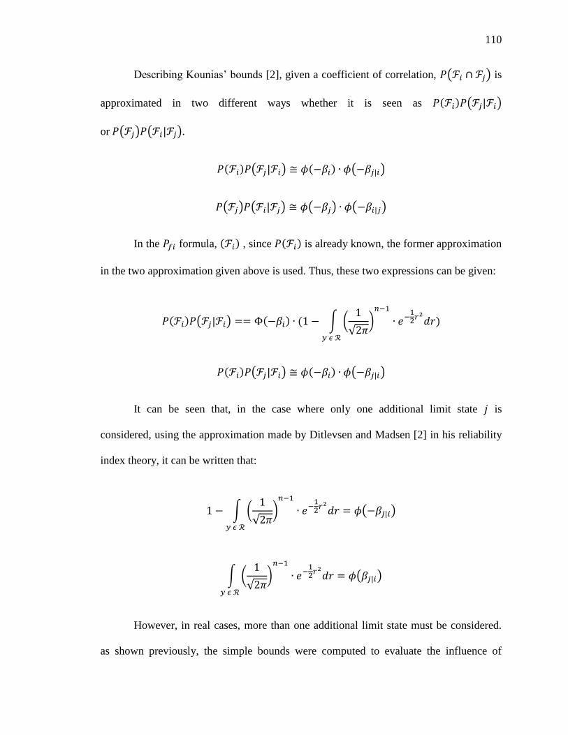
110
Describing Kounias’ bounds [2], given a coefficient of correlation, ( ) is
approximated in two different ways whether it is seen as ( ) ( )
or ( ) ( ).
( ) ( ) ( ) ( )
( ) ( ) ( ) ( )
In the formula, ( ) , since ( ) is already known, the former approximation
in the two approximation given above is used. Thus, these two expressions can be given:
( ) ( ) ( ) ( ∫ (
√ * ;
;
)
( ) ( ) ( ) ( )
It can be seen that, in the case where only one additional limit state is
considered, using the approximation made by Ditlevsen and Madsen [2] in his reliability
index theory, it can be written that:
∫ (
√ * ;
;
( )
∫ (
√ * ;
;
( )
However, in real cases, more than one additional limit state must be considered.
as shown previously, the simple bounds were computed to evaluate the influence of
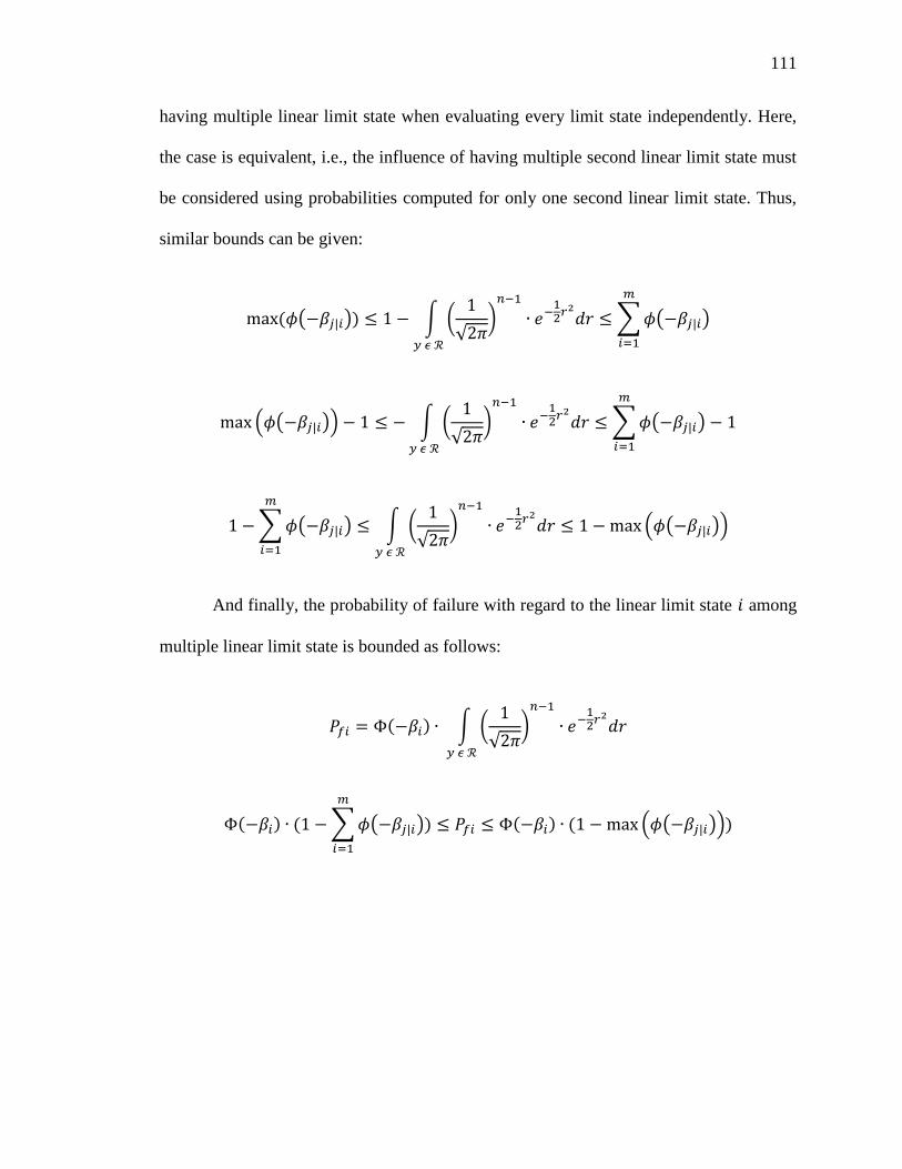
111
having multiple linear limit state when evaluating every limit state independently. Here,
the case is equivalent, i.e., the influence of having multiple second linear limit state must
be considered using probabilities computed for only one second linear limit state. Thus,
similar bounds can be given:
( ( )) ∫ (
√ * ;
;
∑ ( )
<
. ( )/ ∫ (
√ * ;
;
∑ ( )
<
∑ ( )
<
∫ (
√ * ;
;
. ( )/
And finally, the probability of failure with regard to the linear limit state among
multiple linear limit state is bounded as follows:
( ) ∫ (
√ * ;
;
( ) ( ∑ ( ))
<
( ) ( . ( )/)

112
4.7 Material post-failure behavior
It was explained that the over-strength of a structure can be provided by two types
of redundancy. The first one, in a case of indeterminate structures, comes from the
geometry of the structure whereas the second one exists in all structures and comes from
the material. The material redundancy is defined by the material post-failure behavior. In
Chapter 2 of this thesis, it was explained that three categories of material redundancy can
be defined; namely, the capacity in withstanding more displacement, and the capacity in
withstanding more constraints or a combination of both. Hereafter, it will be seen how to
include the post-failure behavior of a material in the reliability model in order to take into
account the material redundancy. It should be noted that the criterion for failure
delimiting the pre-failure behavior and the post-failure behavior is the yielding.
4.7.1 Linear elastic – perfectly plastic model. In this model, the pre-failure behavior
is considered as perfectly elastic and is compatible with a structure analysis such as the
stiffness method. The criterion for failure is the yielding. The post-failure behavior is
perfectly plastic, which means that no additional constraint after yielding can be
withstood by the material. This model can be represented through the strain-stress
constitutive relation curve as depicted in the Fig. 4.24. In this model, when a member has
failed, its strength (the yield stress multiplied by the cross sectional area of the truss
member) can be treated as a new force in the model. However, in the reliability model
used in this thesis, the material characteristics are not taken as random and the force
corresponding to a failed member is not including in the random vector .
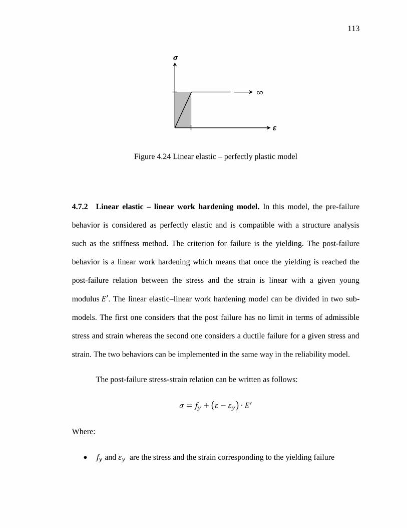
113
Figure 4.24 Linear elastic – perfectly plastic model
4.7.2 Linear elastic – linear work hardening model. In this model, the pre-failure
behavior is considered as perfectly elastic and is compatible with a structure analysis
such as the stiffness method. The criterion for failure is the yielding. The post-failure
behavior is a linear work hardening which means that once the yielding is reached the
post-failure relation between the stress and the strain is linear with a given young
modulus . The linear elastic–linear work hardening model can be divided in two sub-
models. The first one considers that the post failure has no limit in terms of admissible
stress and strain whereas the second one considers a ductile failure for a given stress and
strain. The two behaviors can be implemented in the same way in the reliability model.
The post-failure stress-strain relation can be written as follows:
( )
Where:
and are the stress and the strain corresponding to the yielding failure
𝜺
∞
𝝈

114
is the plasticity modulus
Usually, is small and can be neglected:
A similar relation can be written in term of force and displacement:
( )
And neglecting :
This relation can be implemented in post-failure structural analysis by considering
in the stiffness method a new force equals to at the location of the failed member
and a new stiffness for the member equals to
.
In the stiffness method, the elasticity modulus , is usually not taken into account
because it has no influence since it is usually common to all members. In order to
compute the new stiffness for the member, a new member area could be considered in
order to keep the same .

115
In that way, the post-failure stiffness matrix can be easily computed. It should be
noted that, because the displacement due to the member behavior before yielding is
neglected the structure geometry does not change after a failure. To compute stiffness
after a yielding failure, no additional structural analysis is needed since only the area of
the failed member is modified using a fictive area . This is an important result because
it enables to spare an important number of structural analyses.
The two cases can be implemented in the structural analyses the same way.
However, depending on the behavior chosen a criterion for failure has to be selected. In
the first case, which considers an infinite ductility capacity, the member never fails and
its strength is theoretically capable of reaching any level. In that case, the stiffness matrix
never gets singular and the occurrence of a mechanism within the structure is impossible.
Thus, the classical criterion for failure cannot be used and another criterion must be
defined which could be, for example, the deflection of a given point in the structure.
Indeed, since the failure structure of the structure does not occurs with regard to the
material and a geometric failure criterion must be defined. A criterion based on the
deflection of a given based does not require any additional computation when using the
presented stiffness. In the second case, which considers a ductile failure in the member, a
second limit state for the member can be written to represent the ductile failure. This
results in longer failure paths since each member fails twice. The figure 4.25(a)
represents the case where the material has infinite ductility whereas the figure 4.25 (b)
illustrates a material with a ductile failure.

116
Figure 4.25 Linear elastic – linear work hardening model
4.8 The linear limit state approximation
4.8.1 Introduction to convex sets. A convex set is a set which has the property that if
and belong to the safe set, for every in the interval , -, ( )
belongs to the set. Convex safe sets are particularly convenient for reliability analysis
because any limit state having a convex safe set can be described as the intersection,
finite or infinite, of linear limit states. Thus a model including multiple linear limit states
as presented before can approximate any convex sets and the methods described above
can be used. Ditlevsen and Madsen in [2] provide two methods to approximate any
convex sets to an intersection of multiple linear limit states depending on the curvature of
the convex set (figures 4.26, 4. 27 and 4.28).
𝜺
∞
𝝈
𝜺
𝝈
(a) Infinite ductility (b) Ductile failure

117
Figure 4.26 Convex safe set
Figure 4.27 FORM approximation [2]
Safe set
Failure set
Limit state
𝑿𝟐
𝑿𝟏
Safe set
Failure set
𝑿𝟐
𝑿𝟏
𝜷𝟏
𝜷𝟐

118
Figure 4.28 SORM approximation [2]
Figure 4.26 depicts a convex safe set. Figure 4.27 introduces the first order
reliability method (FORM) approximation. This approximation recognizes that the most
essential contributions to the failure probability come from the vicinities of the most
central point in a case of linear limit states. It is possible to approximate a convex safe set
when the curvature is small by hyperplanes, which remains close to the convex limit state
in the vicinity of the most central point. For a given number of hyperplanes chosen to
approximate the convex safe set, the linear limit states must be chosen to minimize the
probability of failure in order to give the best approximation. F introduces the second
order reliability method (SORM) approximation, which is a correction of the FORM
approximation when the curvature of the limit state surface is considered. The
hyperplanes are shifted toward the inside of the safe set in order to correct the error made
by the FORM assumption.
Safe set
Failure set
𝑿𝟐
𝑿𝟏
𝜷 𝟏
𝜷 𝟐

119
4.8.2 Limit state equation for a single member. In most cases, the member limit state
can be written in term of the loading effects on the member and the member
resistance .
( ) ( ) ( )
is the input variable vector which represents the randomness associated with the
model, i.e. the structure geometry and materials properties and the loading.
Usually, when there is no interaction between the loading and the member
resistance, ( ) is only a function of the member geometry and material characteristics.
( ) ( )
is a family of the input variable vector which is enough to represent
the structure geometry and materials characteristics
Although, the loading effects on the member ( ) is a function of the structure
and the loading, the linear behavior with regard to the loading of a structure enables to
write ( ) using two different functions on two different family of the input variable
vector .
( ) ( ) ( )
( ) ( ( ) ( )) ( )

120
Thus, it is seen that the limit state for a member can be written using function
having for domain the set of distinct family of the input variable vector .
4.8.3 Linear limit state approximation. The linear limit state approximation, which is
widely used in this method, consists in considering that only the load is a random
variable. The random variables describing the structure geometry and materials property
are approximated to be constant. These variables are involved in the member resistance
and in the loading effects on the member. Recognizing that these variables are actually
random variables, they are taken equals to their expected value as follows:
( ) ( ( )) (
( )
( ))
And:
( ) ( ( ) ( )) (
+
( ) ( ( ( )) ( ( ))) (
+
Using this approximation, a linear limit state for a given member is written. It is
reasonable to make this approximation because usually the variability associated with the
load is larger than the variability associated with the structure. In the case of independent
variables, as presented in Fig. 5.29, when a limit state is overpassed, it is usually because
a variable had an occurrence far from its expected value, whereas all the other variables
had occurrences close to their expected values. Since, the loading is the variable with the

121
largest variability, it is considered that the loading is the only candidate to overpass a
limit state while the other variable are taken equals to their expected value. This
approximation is depicted by the Fig. 4.29.
Figure 4.29 Linear limit state approximation and variables scatter
Figure 4.29 depicts a case where the load effect is represented by only one
variable and the resistance of the member is represented by a single variable as well. It
can be seen that most of the time, when an occurrence of the random vector is in the
failure set, the loading variable is far from its expected value; whereas the structure
variable is close to its expected value. This motivates the approximation that only the
loading variability can be taken into account. Thus, the structure’s variables can be
replaced by its expected value and a linear limit state is defined in terms of the loading
variable. In the case presented by Fig. 5.29, the loading variable must be located between
a and b which are the intersection between the limit state and the expected value of the
structure’s variables.
Safe set
Failure set
Limit state
𝒙𝒍𝒐𝒂𝒅𝒊𝒏𝒈
𝒙𝒔𝒕𝒓𝒖𝒄𝒕𝒖𝒓𝒆
𝑬(𝒙𝒍𝒐𝒂𝒅𝒊𝒏𝒈 𝒙𝒔𝒕𝒓𝒖𝒄𝒕𝒖𝒓𝒆)
a b
𝒙

122
4.9 Framework of analyses
One of the purposes of this method was to use the classical framework presented
in the chapter 3. This framework consists in two principal analyses; namely, a structural
analysis and a reliability analysis. The former does not differ in this method but the latter
was modified in order to avoid the issues and inconstancies raised by the classical
methods.
The inputs of the structural analyses are the structure and the loading and the
outputs are the limit state equations for all members. The structural analyses are
conducted using the stiffness method. The inputs of the reliability analyses are the limit
states equations and the random variables of the load and the outputs are, for each
member, the probability of failure, the most central failure point and a new geometry for
the structure. The reliability analyses are conducted using the hybrid method introduced
in this chapter.
The new geometry of the structure is used as a revised input for a new structural
analysis. The knowledge of the most failure point enables to update the random variables.
The probabilities of failures are stored for a post analysis (figure 4.30).
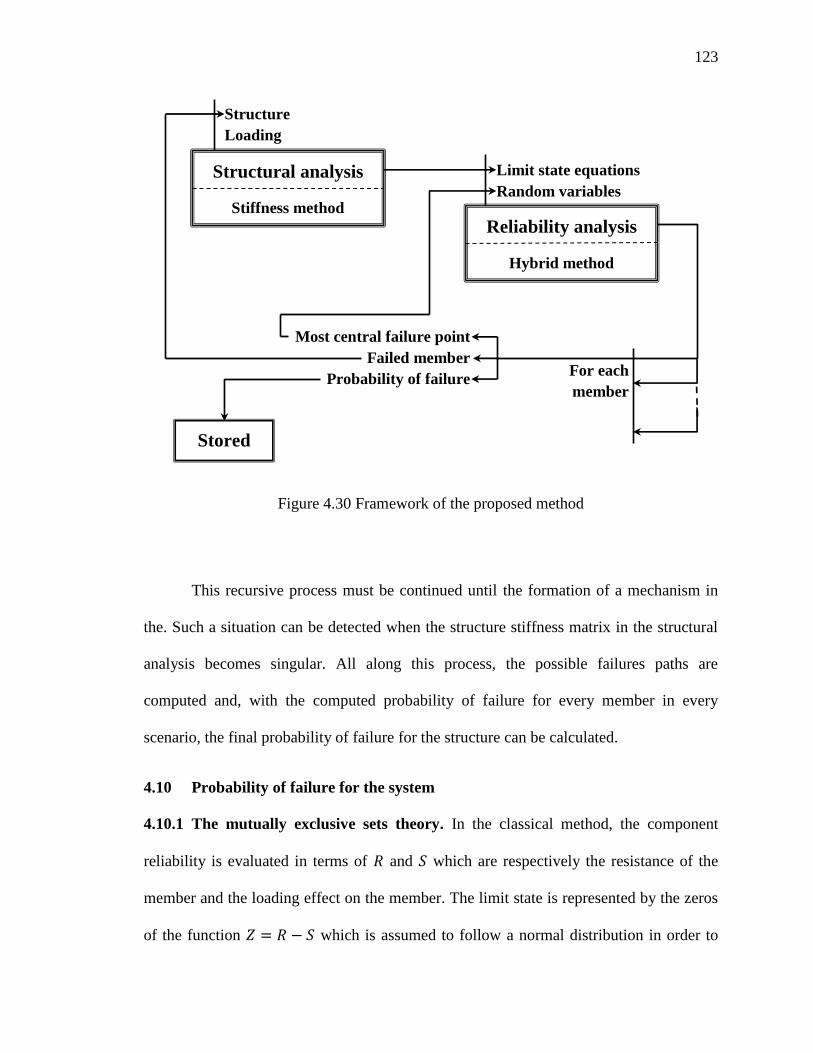
123
Figure 4.30 Framework of the proposed method
This recursive process must be continued until the formation of a mechanism in
the. Such a situation can be detected when the structure stiffness matrix in the structural
analysis becomes singular. All along this process, the possible failures paths are
computed and, with the computed probability of failure for every member in every
scenario, the final probability of failure for the structure can be calculated.
4.10 Probability of failure for the system
4.10.1 The mutually exclusive sets theory. In the classical method, the component
reliability is evaluated in terms of and which are respectively the resistance of the
member and the loading effect on the member. The limit state is represented by the zeros
of the function which is assumed to follow a normal distribution in order to
Structural analysis
Stiffness method
Structure
Loading
Reliability analysis
Hybrid method
Limit state equations
Random variables
For each
member
Most central failure point
Failed member
Probability of failure
Stored

124
compute the probability of failure. Analogously, using the limit state theory introduced in
the beginning of this chapter could be seen as the surface separating the safe set and the
failure set for a given member. The failure would be caused by the occurrence of a vector
describing the structure and its loading in the failure set. Pursuing the analogy for an
entire structure, in a set composed by the domain of definition of all the structure
variables, all the limit states could be represented by a surface separating a safe set and a
failure set. In this case, because the failure sets for different members intersect each
other, it is said that the limit states are correlated. The classical methods do not deal with
the correlation and consider limit state alone in order to compute the probability of failure
of a given member. However the correlation is recognized and taken into account when
computing the probability of failure for the structure, which is bounded by the two
extreme opposite cases where the failure paths are either considered to be entirely
correlated or totally independent.
Contrary to the classical methods, the improved method, using the linear state
approximation, takes the correlation between member failures into account at the member
level. The bounds which are proposed in the hybrid method for the probability of failure
of a given member among multiple intersecting member failure sets are close enough and
one can choose any of them as a good approximation for the actual member probability
of failure. Since, there is no reason to prefer any of the two bounds, the member
probability of failure is assumed to be the average of the two bounds. In this method, the
member failure probability corresponds to the occurrence of a vector representing the
loading in the member failure set which is made mutually exclusive from the other
125
member failure sets by using the load continuity hypothesis. Thus, the member failure
sets are a partition of the failure set.
When a member failure occurs, the structure geometry and the random
characteristic of the loading are updated. A new failure set is shaped and partitioned with
mutually exclusive sets corresponding to the member failure sets. The probability of
failure for a second given member is the probability of the updated random variable to
occur in the mutually exclusive failure set corresponding to the considered member in the
new structure failure set (see figure 4.31).
Finally, the occurrence of a failure path corresponds to the successive occurrences
of the successive random input variables in the member failure sets defined on the
updated structure failure sets given the history of failure. All these member failure sets
are mutually exclusive. The characteristic of the random input variables are defined in
function of the scenarios in which they are. It should be noted that these variables are
independent from each other.

126
Figure 4.31 Successive mutually exclusive sets
4.10.2 Probability of failure of the structure. The probability of failure can be
computed by determining the probability of failure of all failure paths. The occurrence of
a failure path corresponds to the occurrence of a given number of independent variables
in mutually exclusive failure sets. These independent variables can be taken as a single
variable representing all the outcome of the variables along the failure path. The union
of these mutually exclusive sets can be considered as the failure path set . The
probability of occurrence of a failure path is written as follows:
( ) ( ) ( ) ( ; ; )
Where:
is the family of corresponding to the variable defined at the stage in the
failure path.
Intact structure failure set
𝒊
Structure failure set with member i failed
𝒋
𝒌
member 𝒊 failure
𝒋

127
is the subset of corresponding to the member failure set at the stage in the
failure path.
The two bounds given in the hybrid method give are close and the average of the
two bounds can be used as a good approximation for the probabilities.
Finally, since the failure paths set are composed of mutually exclusive, these sets
are also mutually exclusive. Thus, the probability of failure is the sum of the probabilities
of occurrence of all the failure paths.
( ) ∑ ( )
Where:
corresponds to the variable representing all the outcome of the variables along
the failure path .
is the failure path set corresponding to the failure path .
4.11 Concluding remarks
The method reviewed herein successfully overcomes the major shortcomings of
the classical method and offers several improvements. These improvements are: (1) The
correlation among member failures is taken into account by using mutually exclusive
failure event. (2) The load is updated to be more consistent with a real situation thanks to
the most failure point. (3) The calculations are faster because unnecessary and

128
inconsistent limit states are removed. (4) Strategies are proposed to take into account
material redundancy, i.e. plasticity.
However, the method has its own shortcomings. These are: (1) The limit states
must be linear or approximated to be linear. (2) The mutually exclusive events are based
on an approximation. (3) The randomness of the structure characteristics is ignored.
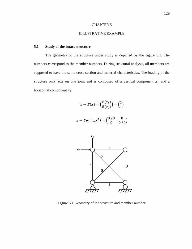
129
CHAPTER 5
ILLUSTRATIVE EXAMPLE
5.1 Study of the intact structure
The geometry of the structure under study is depicted by the figure 5.1. The
numbers correspond to the member numbers. During structural analysis, all members are
supposed to have the same cross section and material characteristics. The loading of the
structure only acts on one joint and is composed of a vertical component and a
horizontal component .
( ) ( ( )
( )* .
/
( ) .
/
Figure 5.1 Geometry of the structure and member number
𝒙𝟏
𝒙𝟐
𝟏
𝟐
𝟑
𝟒
𝟓
𝟔
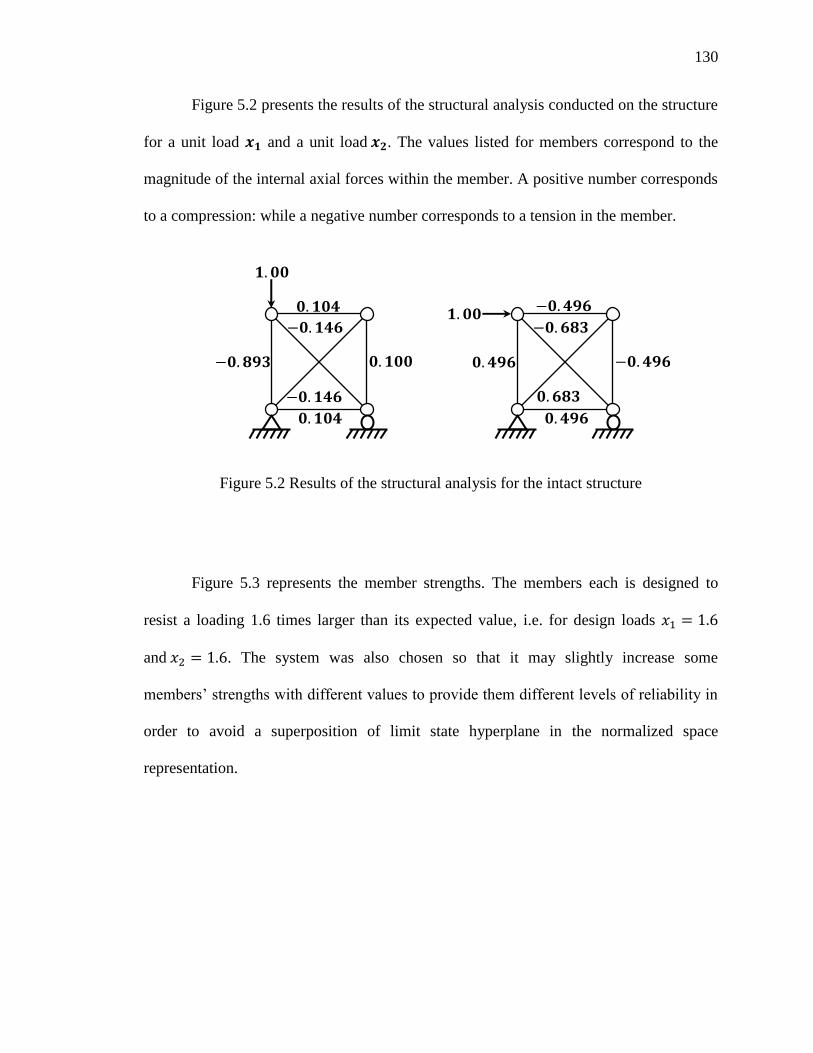
130
Figure 5.2 presents the results of the structural analysis conducted on the structure
for a unit load and a unit load . The values listed for members correspond to the
magnitude of the internal axial forces within the member. A positive number corresponds
to a compression: while a negative number corresponds to a tension in the member.
Figure 5.2 Results of the structural analysis for the intact structure
Figure 5.3 represents the member strengths. The members each is designed to
resist a loading 1.6 times larger than its expected value, i.e. for design loads
and . The system was also chosen so that it may slightly increase some
members’ strengths with different values to provide them different levels of reliability in
order to avoid a superposition of limit state hyperplane in the normalized space
representation.
𝟏 𝟎𝟎
𝟎 𝟏𝟎𝟒
𝟎 𝟖𝟗𝟑
𝟎 𝟏𝟒𝟔
𝟎 𝟏𝟒𝟔
𝟎 𝟏𝟎𝟒
𝟎 𝟏𝟎𝟎
𝟏 𝟎𝟎 𝟎 𝟒𝟗𝟔
𝟎 𝟒𝟗𝟔 𝟎 𝟒𝟗𝟔
𝟎 𝟒𝟗𝟔
𝟎 𝟔𝟖𝟑
𝟎 𝟔𝟖𝟑

131
Figure 5.3 Member strengths
With the member strengths known and the structural analysis performed, it is
possible to write the member limit states as follows:
{
( ) ( ) ( ) ( ) ( )
( )
It should be noted that a unique mode of failure is chosen for each member. This
mode of failure is either a compression failure or a tension failure depending on the sign
of the force within the member for the expected values of and . The limit state can
be written in the normalized space using the following transformation.
𝟎 𝟕𝟏𝟎
𝟎 𝟖𝟎𝟎 𝟎 𝟔𝟓𝟎
𝟏 𝟏𝟓
𝟏 𝟒𝟓𝟎
𝟎 𝟗𝟐𝟎

132
And, in the normalized space:
{
( ) ( ) ( ) ( ) ( ) ( )
Figure 5.4 is the representation of these limit states in the normalized space.
Figure 5.4 Limit states in the normalized space for the intact structure
As was discussed in the chapter 5, from the first representation of all limit states
in the normalized state, it can be seen that some limit states are not consistent with reality
because of the continuous evolution of the load. In that case, the limit states of members
-4
-3
-2
-1
0
1
2
3
4
-1 0 1 2 3 4 5 6 7
Member 1
6 3 5
2
4
Safe Set 𝒚𝟏
𝒚𝟐

133
2, 4, 5 and 6 do not represent possible failures and should be removed. Figure 5.5 is a
consistent representation of the possible failures within the structure.
Figure 5.5 Consistent limit states for the intact structure
It is possible, by using the index and by integrating on the hyperplane, to
calculate the probability of failure for the member 1 and for the member 3. The results
are summarized in the Table 5.1.
-4
-3
-2
-1
0
1
2
3
4
-1 0 1 2 3 4 5 6 7
Member 1
Member 3
𝜷
𝜷𝟑
𝒚𝟏
𝒚𝟐

134
Table 5.1 Probability of member failure for the intact structure
Member ( ) ∫ (
√ * ;
;
1 1.61 0.0537 1 0.0537
3 1.41 0.0793 1 0.0793
As shown in Fig. 5.5, among the 6 possible failures only two must be considered.
In order to update the characteristics of the loading for further analyses, the most central
failure points for the failure of the member 1 and for the failure of the member 3 must be
computed (see Table 5.2).
Table 5.2 Most central failure point for the intact structure
Member In the normalized space In the loading space
1
3
5.2 Study of the structure with the member 1 failed
The loading of the structure is composed of three forces. The two first forces are
the random loadings which have the following updated characteristics:

135
( ) ( ( )
( )* .
/
( ) .
/
And the last force corresponds to the plastic force within the member 1 which has
a value of 0.800. Figure 5.6 presents the results of the structural analysis conducted on
the structure for a unit load and a unit load . Figure 5.7 represents the forces in the
structures caused by the member 1 plastic force.
Figure 5.6 Results of the structural analysis for the structure with member 1 failed
Figure 5.7 Forces in members caused by the member 1 plastic force
𝟏 𝟎𝟎
𝟎 𝟗𝟖𝟔
𝟏 𝟑𝟗
𝟏 𝟑𝟗
𝟎 𝟗𝟖𝟔
𝟎 𝟗𝟕𝟑
𝟏 𝟎𝟎 𝟎 𝟗𝟗𝟓
𝟎 𝟗𝟖𝟑
𝟎
𝟏 𝟒𝟎
𝟎
𝟎 𝟖𝟎𝟎
𝟎 𝟕𝟖𝟗
𝟎 𝟕𝟕𝟖
𝟎 𝟕𝟖𝟗
𝟏 𝟏𝟐
𝟏 𝟏𝟐

136
At this stage, the member strengths are still the same; and upon structural
analysis, it is possible to write the member limit states as follows:
{
( ) ( )
( ) ( )
( )
These limit states can be written in the normalized space using the following
transformation:
And, in the normalized space,
{
( ) ( )
( ) ( )
( )
Figure 5.8 is a representation of these limit states in the normalized space.

137
Figure 5.8 Limit states in the normalized space for the structure with member 1 failed
From Fig. 5.8, it is possible to detect which limit states are not consistent and to
plot a consistent representation of the situation (see Fig. 5.9).
-2
-1
0
1
2
3
4
5
-2 -1 0 1 2 3 4 5
𝟒
𝟓 𝟔
𝟑
Safe Set 𝒚𝟏
𝒚𝟐

138
Figure 5.9 Consistent limit states for the structure with member 1 failed
Again, by using the index and by integrating on the hyperplane, the probability
of failure for the member 5 and for the member 6 are computed. The results are
summarized in Table 5.3.
Table 5.3 Probability of member failure for the structure with member 1 failed
Member ( ) ∫ (
√ * ;
;
5 1.26 0.104 1 0.104
6 3.14 0.000840 1 0.000840
-2
-1
0
1
2
3
4
5
-2 -1 0 1 2 3 4 5
T pez u e équ t Member 5
Member 6 Member 5
𝜷𝟓 𝜷𝟔 <
𝒚𝟏
𝒚𝟐
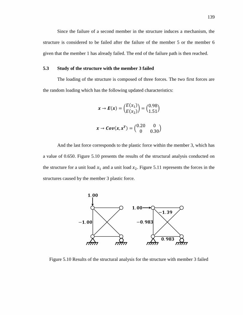
139
Since the failure of a second member in the structure induces a mechanism, the
structure is considered to be failed after the failure of the member 5 or the member 6
given that the member 1 has already failed. The end of the failure path is then reached.
5.3 Study of the structure with the member 3 failed
The loading of the structure is composed of three forces. The two first forces are
the random loading which has the following updated characteristics:
( ) ( ( )
( )* .
/
( ) .
/
And the last force corresponds to the plastic force within the member 3, which has
a value of 0.650. Figure 5.10 presents the results of the structural analysis conducted on
the structure for a unit load and a unit load . Figure 5.11 represents the forces in the
structures caused by the member 3 plastic force.
Figure 5.10 Results of the structural analysis for the structure with member 3 failed
𝟏 𝟎𝟎
𝟏 𝟎𝟎
𝟏 𝟎𝟎
𝟎 𝟗𝟖𝟑
𝟎 𝟗𝟖𝟑
𝟏 𝟑𝟗

140
Figure 5.11 Forces in members caused by the member 3 plastic force
The member strengths are still the same; and upon structural analysis, it is
possible to write the member limit states as follows:
,
( ) ( ) ( )
Again, these limit states can be written in the normalized space using the
following transformation:
And, in the normalized space,
,
( ) ( ) ( )
Figure 5.12 is a representation of these limit states in the normalized space.
𝟎 𝟔𝟓𝟎
𝟎 𝟔𝟒𝟏
𝟎 𝟔𝟒𝟏
𝟎 𝟗𝟎𝟔
𝟎 𝟗𝟎𝟔
𝟎 𝟔𝟑𝟐

141
Figure 5.12 Limit states in the normalized space for the structure with member 3 failed
Again, using Fig. 5.12, it is possible to detect which limit states are not consistent
and to plot a consistent representation of the situation (see figure 5.13).
-3
-2
-1
0
1
2
-1 0 1 2 3 4 5
𝟔 𝟒
Safe Set 𝒚𝟏
𝒚𝟐

142
Figure 5.13 Consistent limit states for the structure with member 3 failed
Again, by using the index and by integrating on the hyperplane, the probability
of failure for the member 1 and for the member 6 are calculated. The results are
summarized in Table 5.4.
-3
-2
-1
0
1
2
-1 0 1 2 3 4 5
Member 1
Member 6
𝜷
𝜷𝟔
𝒚𝟐
𝒚𝟏

143
Table 5.4 Probability of member failure for the structure with member 3 failed
Member ( ) ∫ (
√ * ;
;
1 1.91 0.0281 1 0.0281
6 0.61 0.271 1 0.271
Since the failure of a second member in the structure induces a mechanism, the
structure is considered to have failed after the failure of the member 1 or the member 6
given that the member 3 has already failed. The end of the failure path is therefore
reached.
5.4 Structure probability of failure
The structure probability of failure is based on the occurrence of failure paths.
The probability of occurrence of a failure path is taken as the multiplication of the
probability of failure of all members involved in the failure path. Table 5.5 gives the
probability of occurrence of the possible failure paths.

144
Table 5.5 Probability of occurrence of failure paths
Failure path Probability of occurrence
(1,5) ;
(1,6) ;
(3,1) ;
(3,6) ;
Finally, the structure probability of failure is taken as the sum of the probability of
occurrence of all failure paths.
; ; ; ; ;
The failure paths can be represented in a tree as depicted by Fig. 5.14.

145
Figure 5.14 Failure paths tree for the example structure
1
1
3
6
5
6
;
;
;
;
𝑃𝑓 ;

146
CHAPTER 6
SUMMARY AND CONCLUSIONS
6.1 Summary
This thesis presents an overview of an improved method that can be used for the
probabilistic evaluation of the redundancy in indeterminate trusses. The improved
method offers advantages over classics method by considering:
An approximation to make the events of member failures mutually exclusive.
Geometric calculations to determine reliability indices and conditional reliability
indices in order to establish closer bounds for the failure probability of individual
structural members.
System’s failure probability using the assumption and procedures outlined in (1)
and (2) above.
Further extending the method beyond geometrical redundancy by using material
redundancy, and plasticity models commonly used in the structural analyses.
The details of the improved methods, as provided in literature, are provided in the
thesis. A numerical example is presented to demonstrate the sequence of failure in a truss
system and how various improvements can be used to arrive at the probability of system
failure for a simple redundant truss. The purpose of this example is only to demonstrate
the methods reviewed herein without any specific comments in terms of any design
recommendations. The following are the main conclusions of the study:

147
The improved method for probabilistic evaluation of structural redundancy can be
applied to redundant systems by considering geometrical and material
redundancies.
Certain approximation regarding the failure limit states and formulation of
probability can be made to make the method efficient. Among these include
removal of members with significantly low probability of failure in individual
failure paths.
The incorporation of material redundancy and geometrical properties as well as
consideration of possible failures among members are expected to provide more
accurate results than those using classical methods.
6.2 Recommendations for further studies
The following studies are proposed for the extension of this research.
Conduct the analysis for several real trusses to investigate their redundancy
though the improved method.
Develop software to automatically identify failure paths in reducing the
computation effort.
Apply classical methods for these trusses to develop a baseline for comparing
results from the improved method.
Suggest specific case studies where the load can change during member failures,
as indicated in the improved method.
148
BIBLIOGRAPHY
[1] American Association of State Highway and Transportation Officials, ed. Standard
Specifications for Highway Bridges 17th Edition. N.p.: AASHTO, 2002. Print.
[2] Ditlevsen, O., and H. O. Madsen. Structural Reliability Methods. N.p.: Technical
University of Denmark, 2007. Print. [3] Frangopol, D. M., and J. P. Curley. "Effects of Damage and Redundancy on
Structural Reliability." Journal of Structural Engineering 113.7 (1987): n. pag.
Print.
[4] Gharaibeh, E. S., D. M. Frangopol, and T. Onoufriou. "Reliability-based
Importance Assessment of Structural Members with Applications to Complex
Structures." Computers and Structures 80 (2002): n. pag. Print.
[5] Ghasemi, M. R., and M. Yousefi. "Reliability-based Optimization of Steel Frame
Structures Using Modified Genetic Algorithm." Asian Journal of Civil
Engineering 12.4 (2011): n. pag. Print.
[6] Ghosn, M., and F. Moses. Report 406 - Redundancy in Highway Bridge
Superstructures. New York: AASHTO, 1998. Print.
[7] Kalatjari, V., V. Kaveh, and P. Mansoorian. "System Reliability Assessment of
Redundant Trusses Using Improved Algebraic Force Method and Artificial
Intelligence." Asian Journal of Civil Engineering 12.4 (2011): n. pag. Print.
[8] Kanno, Y., and Y. Ben-haim. "Redundancy and Robustness, or When Is
Redundancy Redundant?" Journal of Structural Engineering (2011): n. pag. Print.
[9] Kassimali, A. Matrix Analysis of Structures. 2nd ed. N.p.: Carbondale, 2010. Print.
[10] Kritzler, R. W. "Redundancy Evaluation of Bridge Structure." Thesis. Illinois
Institute of Technology, 1990. Print.
[11] Melchers, R. E., and L. K. Tang. "Dominant Failure Modes in Stochastic Structural
System." Reliability Engineering and System Safety. Elsevier, 2003. Web.
[12] Mohammadi, J., A. Longinow, and S. J. Suen. Probabilistic Evaluation of
Redundancy In Safety Analysis Of Highway Bridges. Tech. Vol. 3. Wroclaw: n.p.,
1987. Print.
[13] Murotsu, Y., S. Matsui, and Q. S. Tong. Contributions to the Systems Reliability of
Structures. Thesis. University of Osaka Prefecture, 1992. Osaka: n.p., 1992. Print.

149
[14] Park, S., S. Choi, C. Sikorsky, and N. Strubbs. "Efficient Method for Calculation of
System Reliability of a Complex Structure." International Journal of Solids and
Structures 41 (2004): n. pag. Print.
[15] Thoft-Christensen, P., and J. M. Baker. Structural Reliability Theory and Its
Applications. N.p.: Springer-Verlag, 1982. Print.