An overview of Human Connectome Project (HCP) database

An overview of Human Connectome

Project (HCP) database

HCP course

HCP Course Attendees: WELCOME!

August 28 – September 1, 2016

Joseph B. Martin Conference Center Boston, MA

Saint Louis University University of Oxford, University d’Annunzio Indiana University, Warwick University Ernst Strungmann Institute (Frankfurt) Radboud University (Nijmegen), Duke University Advanced MRI Technologies (Sebastopol CA)

The “WU-Minn” HCP consortium

HCP is grateful to the NIH Blueprint

10 institutions: Washington University University of Minnesota Oxford University

>>100 HCP consortium members

Course logistics

Cortical cartography• Maps, parcellations • Connectivity – ground truth principles• Variability, atlases, and alignment

Human Connectome Project• History & overview • Methodological highlights and teasers• The HCP-style paradigm

Outline

Human Brain Numbers

Azevedo et al. (J. Comp. Neurol., 2009) Pakkenberg et al. (Exp. Gerontol., 2003)

Whole brain: 1500g; 86 billion neurons1

Cerebellum:• 10% of brain mass• 69 billion neurons (80%)• coordinates movements, thoughts

Rest of brain: • 8% of brain mass• 0.7 billion neurons (0.8%)• vital ‘housekeeping’ functions

Cerebral cortex: ~80% of brain mass (GM + WM); a wide range of functions16 billion neurons (~20%)150 trillion synapses (~10,000/neuron)160,000 km myelinated WM axons (~1 cm/neuron)

Cerebral cortex White matter

Subcortical “nucleus”

Small, medium, and large brains

~200x~15x

3x

Herculano-Houzel(Front. Hum.

Neurosci., 2014)

~3000x

• Dramatic expansion of human brain in last 2 million years

Diverged~5 - 7 MYA

Diverged25 - 30 MYA Diverged

~75 – 100+ MYA

• Cortical convolutions vary enormously. Enter “cortical cartography”

Diverged~35 MYA

Pencil-and-paper flat map(Van Essen & Maunsell, 1980)

Cortical cartography– humble beginnings (pre-MRI)Computerized surface reconstruction

Carman et al., 1995

The Visible Man

Van Essen & Drury, 1997

And then, the MRI revolution began!• Structural MRI (T1w, T2w)• Segmentation algorithms• Functional MRI• Diffusion MRI

Earth maps can display• Geography• Political subdivisions• Lots of other information

Capturing cortical convolutions

HCP structural MRI:• High-quality structural MRI: 0.7 mm voxels • Customized FreeSurfer segmentation (uses

T1w + T2w; now part of FreeSurfer 6.0)

Glasser et al. (Neuroimage, 2013) HCP ‘Pipelines Paper’

• Conventional T1w: 1mm isotropic voxels

• Standard FreeSurfer: good but imperfect

Bruce Fischl

Courtesy John Harwell (and Apple Computer)

A surface-centric perspective

16

Many options for segmentation, surface inflation/flattening:

• Brain Voyager• MNI CIVET• Standard FreeSurfer (e.g., v6.0)• HCP Structural Pipeline (uses FreeSurfer with T1w + T2w)• Many others….

They aren’t equivalent in quality and fidelity.Cortical surface area: 100,000 mm2/hemisphereThickness: 1.5 – 4mm

• ~150K mesh is desirable (<1mm between vertices)• HCP registers to “164k” standard mesh• HCP also downsamples to “32k” mesh, best for fMRI,

connectivity analyses

Parcellation based on “FACTs”:• Function• Architecture• Connectivity• Topography

Many methods(invasive and noninvasive)

Poster children: areas V1, MTBut - most other areas are fuzzy, debatable• Subtle boundaries• Noise and bias in the data• Discordant results from different approaches• Cortical parcellation is really hard!!

Macaque cortical parcellation – the early days

The ’80-G’ atlas

V1

MT

V1 V2

V3?

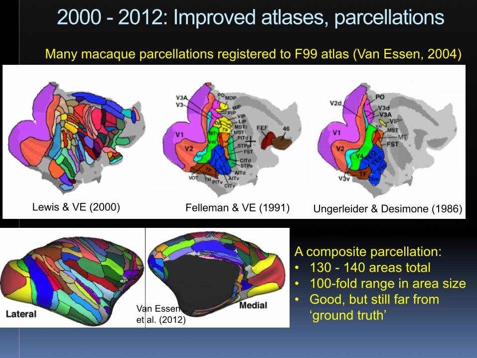
2000 - 2012: Improved atlases, parcellationsMany macaque parcellations registered to F99 atlas (Van Essen, 2004)

Lewis & VE (2000) Felleman & VE (1991) Ungerleider & Desimone (1986)

A composite parcellation:• 130 - 140 areas total• 100-fold range in area size• Good, but still far from

‘ground truth’Van Essen et al. (2012)

19

Human cortical geography

Lobes, gyri and sulciBut highly variable!

Nieuwenhuys et al. (2014)

FreeSurferaparc.a2009s

Human geographic atlases used in neuroimaging:

AAL, other atlases also available. But parcels are not well correlated with functionally distinct cortical areas

Nieuwenhuys et al. (2014);Vogt (1903); O. and C. Vogt (1919) 20

Brodmann (1909)

Human cortical architectonicsCytoarchitecture Myeloarchitecture

(Ongur et al., 2003)

Kujovicet al., 2012

T1-weighted imageT2-weighted imageDivide and conquer:T1w/T2w ratio

Myelin maps in cerebral cortex

MT+

Sensory-motor strip

Auditory

Glasser & Van Essen (2011); Glasser et al. (2013)

darker

brighter

HighLow

Myelin content

brighter

darker

Early myelination:Heavy adult myelination

Matt Glasser

Course logistics


Human Connectome Project• History & overview • Methodological highlights and teasers

Outline

A binary connectivity matrix“parcellated connectome”

Macaque cortical connectivity (1979 - 2000)

Felleman & Van Essen (1991)

Van Essen (1979) Maunsell & Van Essen (1983)

1991: Little quantitative connectivity data available

Connectivity density(MSTd injection)

Lewis & Van Essen (2000) Wide range of conection strengths!

Macaque anatomical tracers (Markov et al., 2012,

2014)

• Average of 55 inputs to each cortical area!

• Connection strengths: > 5 log units(!);

lognormal distribution!

• 29x91 matrix; 1,615 identified pathways!

• Total = ~104 pathways (cortical + subcortical)

Cortical Connectivity: ‘ground truth’ in macaque

Tracer inArea 7A

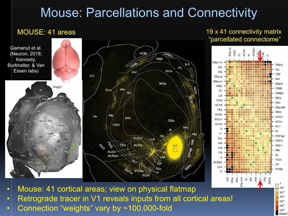
Mouse: Parcellations and Connectivity

• Mouse: 41 cortical areas; view on physical flatmap

• Retrograde tracer in V1 reveals inputs from all cortical areas!

• Connection “weights” vary by ~100,000-fold

MOUSE: 41 areas 19 x 41 connectivity matrix

“parcellated connectome”

Gamanut et al.

(Neuron, 2018;

Kennedy,

Burkhalter, & Van

Essen labs)

Course logistics



Outline

W, X = twins

Y, Z = twins

Human Cortical Convolutions

• Convolutions are complex!• Highly variable across individuals• More variable in ‘higher cognitive’ regions• Variable even in identical twins, but some heritability• HCP: MZ, DZ twins & siblings

Botteron, Dierker, Todd et al. (OHBM 2008)

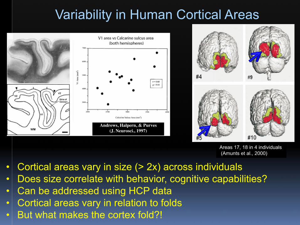
Areas 17, 18 in 4 individuals(Amunts et al., 2000)

Variability in Human Cortical Areas

• Cortical areas vary in size (> 2x) across individuals• Does size correlate with behavior, cognitive capabilities?• Can be addressed using HCP data• Cortical areas vary in relation to folds• But what makes the cortex fold?!

Andrews, Halpern, & Purves(J. Neurosci., 1997)

Coogan & Van Essen (1996)

• Consistent folding in regions dominated by major pathways• Variable folding in ‘balkanized’ regions (small areas, variable connectivity)• One of multiple mechanisms? (also ‘buckling’, differential proliferation?)

25 week 30 week 33 week 37 week 4 yearsHill et al. (2010)

Tension-based Cortical Folding? (Van Essen - Nature,1997)

Macaque V1, V2 differentiate while cortex is smooth; gyrus in between forms later

Gyrus forms as major, topographic V1-V2 pathway is established (~E108)

An aha moment!

Cortical folding: mainly prenatal, as connections are established

V1

V2

V1

V2

Volume-based registration to an atlasMultiple target options (e.g.,Talairach vs group average MRI)• Even nonlinear registration doesn’t align all gyri, sulci• Beware of ‘drift’: MNI152 = 137% average individual volume• Smoothing in volume blurs across cortical ribbon boundaries

FSL FNIRT (nonlinear)

Individual0

500

1000

1500

2000

Native MNI

Cubi

c Ce

ntim

eter

s

HCP 196 Brain Volumes

A typical task-fMRI contrast

Surface-based registration for accurate cortical alignment

Case 1 Case 2FSL’s ‘FNIRT’

atlas

volume registration

Surface-based registration‘fsaverage’ atlas

FreeSurfer shape-based spherical registration

Multiple spherical registration methods• FreeSurfer algorithm is good but not perfect

o Large ‘non-biological’ distortionso Residual misalignment of functional areas

• Recent improvements: left-right correspondence; multimodal surface matching

fsaveragehemispheres NOT

in register

‘fs_LR’ hybrid atlas:best of both worldsThe “fs_LR” mesh aligns

FreeSurfer left & right hemispheres

Accurate interhemispheric alignment: essential for evaluating hemispheric symmetries, asymmetries

Van Essen et al. (2012b)

A composite surface-based human

cortical parcellation

Van Essen et al. (2012b)

‘Entry requirements’:

• Well-defined cortical areas

• Accurately mapped to individual surfaces

• Accurately registered to a surface-based atlas

Available in 2012:

• Observer-independent architectonic (Fischl et al., 2008)

• Orbito-frontal multi-modal architectonic (Ongur et al.

2003)

• Retinotopic fMRI (Swisher et al., 2010; Kolster et al., 2010;

Brewer et al., 2005)

52 surface-mapped areas, 1/3 of hemisphere

Total: ~150 – 200 areas?

How to fill in the gaps? Stay tuned for this afternoon!

Improving Intersubject Alignment

Multimodal Surface Matching (MSM) can do this!Emma Robinson, Mark Jenkinson et al. (2013, 2014, 2018)

• Stay tuned!

V1 Max Overlap 100%

MT+ (hOc5) Max Overlap 50%

Shape-based alignment (FreeSurfer): • performs well where folding is consistent• poorly where folding is variable and area-folding correspondence is weak

A vision:“In the future, it will be desirable to incorporate reliable functionally based landmarks along with geographic information in driving the transformations. “ (Drury et al., 1996)

Compared to cerebral cortex:• Convolutions are more regular (lobules, lamellae, folia)• Cortex is thinner (<1mm vs 2.6mm average)• Much less white matter (NO cortico-cortical connections!)• Large surface area (>1,000 cm2) despite small volume• Hemispheres joined at midline - one sheet, not two!• Automated segmentation not feasible (even on HCP MRIs)• Can map data to ‘colin’ atlas cerebellar surface

Cerebellar cortex is special!

HCP subject 100307Coronal Sagittal

‘Colin’ atlas(Van Essen, 2004)

Course logistics

Cortical cartography• Maps, parcellations• Connectivity – ground truth principles• Variability, atlases, and alignment


Outline

§ For the human brain, focus on the macro-connectome

What’s a connectome?§ A “comprehensive” map of neuronal connections

Macro-connectomewhole-brain, long-distance Micro-connectome

(synapses, neurons)

Triple connectomes!

38

Meso-connectomeCellular + long-distance

Mouse area V1 connections(Wang & Burkhalter, 2008)

Volume reconstructed: <1 mmVoxels: 1 – 2 mm Many injections, many brains

Human Connectome Project: a brief history• May, 2009: Request for Applications from NIH “Blueprint”• September, 2010: NIH awards to two HCP consortia

• $30M to “WU-Minn” consortium• Two+ years of methods development + piloting• Data acquisition:

WashU (3T, 100 mT/m), UMinn (7T), SLU (MEG)• Target: 1200 subjects (twins + siblings)• Analysis: Oxford (fMRI, dMRI); MEG (Chieti, Frankfurt, Nijmegen)

• “MGH/UCLA” consortium (MGH scanner with 300 mT/m gradients) • 2013: “Lifespan Pilot” supplements to WU-Minn, MGH consortia

39

1) Acquire data on brain structure, function, and connectivity in healthy adults (twins and non-twin siblings).

•  Improved scanners, pulse sequences•  Multimodal imaging (~4 hours total scan – 4 x 1h sessions)•  Data quality: exceptionally high!•  1200 subjects studied, ~1100 with MRI (completed September, 2015)•  184 subjects scanned at 7T (completed November, 2015)•  Behavioral data (478 ‘subject measures’) •  Magnetoencephalography (95 subjects): Task-MEG, resting-state MEG •  Blood for genotyping (to dbGAP in fall, 2016)

2) Analyze the data•  Improved HCP preprocessing pipelines•  Better visualization (Connectome Workbench)•  Advanced analyses

43

HCP Behavioral tests

• NIH Toolbox; Penn Neuropsychological Battery• Diverse phenotypes

• Cognition• Emotional health• Motor skills• Sensory• Personality• Fluid intelligence• Family environmental factors

• Demographic, physical data• Psychiatric status, substance use• Some data are Restricted Access (separate Data Use Terms)

Sensory: Which feels different?Cognitive: Match the shape

41

Personality – NEO-FFI (neuroticism)

Deanna Barch

3) Share the HCP data§  ConnectomeDB database – a robust infrastructure §  900-subject data release (June, 2015) §  7T subjects (73 subjects, Part 1 – June, 2016) §  MEG data release (95 subjects, November, 2015) §  1100-subject release - fall, 2016 §  >6,000 investigators accepted HCP Data Use Terms (~600 Restr. Access) §  >10 petabytes (10,000 TB) of HCP data shared (7 PB downloaded, 3

PB in hard drives shipped) §  Release of extensively analyzed data

ConnectmeDB: ‘Network matrices’; ‘MegaTrawl; dense connectome) BALSA database: Glasser et al., 2016 (Nature; Nature Neuroscience)

§  >140 publications using HCP data §  HCP website: www.humanconnectome.org

45

The HCP-style Neuroimaging ParadigmSeven core tenets (Glasser et al. Nature Neuroscience, 2016)

1) Collect lots of multimodal imaging data. 2) Maximize resolution, data quality (e.g., multiband fMRI, dMRI)

3) Minimize distortion and blurring of each subject’s data4) Respect geometry of brain structures (‘CIFTI grayordinates’).

5) Align data precisely across individuals and across studies.6) Analyze results using an accurate brain parcellation.7) Freely share the data (including publication-related data).

CIFTI “Grayordinates”

For gray-matter analyses (e.g., fMRI): §  Cortex plus subcortical gray matter only §  Appropriate geometric models

ú  Cerebral cortex: surfaces, vertices ú  Subcortical: volumes, voxels ú  Cerebellar cortex: voxels (for now)

§  Intersubject alignment: ú  Cortex: surface registration ú  Subcortical: nonlinear volume-based

§  Spatial smoothing in grayordinates space (avoid blurring outside cortical ribbon)

Glasser et al (2013) Neuroimage “HCP Pipelines Paper”

HCP Advances: Representation and Alignment

The HCP atlas approach • A “CIFTI-based” composite coordinate system:

• Grayordinates = cerebral cortex surface vertices + subcortical gray-matter voxels

• Whiteordinates = white matter voxels (for tractography)

• Surface alignment (individuals to atlas)• Folding-based (MSMSulc) – ok but blurry task-fMRI assay• Much sharper for areal feature-based alignment (MSMAll)

• Enabled a new multimodal cortical parcellation

“CIFTI” format:grayordinates(vertices + voxels)

Social Cognition

Social Random

HCP Task-‐evoked functional MRI Language

Listen to short stories; Answer questions about the story

Story Math Do arithmetic problems

•  Seven tasks (1 hr scan time) •  Extensive brain coverage •  Diverse functional systems

Working Memory

Faces, Places, Bodies, Tools

3

Whole-‐brain visualization

Left Cerebellar flat map

anterior

posterior

ventral Medial Lateral

Right

‘Colin’ cerebellum

activationdeactivation

HCP Task-fMRI activations

• ‘Story’ task language activations: bilateral but L > R• Patchy cerebellar activations, R > L



‘Social interaction’ vs. random: overlap (prefrontal) + distinct occipito-temporal



• Working memory (2-back vs 0-back): prefrontal, cingulate, & cerebellar

• Different tasks engage complex, partially overlapping networks

BOLD fMRI time course

(locations 1, 2)

Functional connectivity map

(location 2)

Functional connectivity from R-fMRI correlations

•

Functional connectivity map

(location 1)

HighLow

Correlation

Functional connectivity

matrix (‘dense

connectome’)

30 GB = 90k x 90k ‘grayordinates’)

Correlate time series

HCP resting-state networks (RSNs)

Independent Components Analysis (ICA) [Smith, Beckmann et al.]• Spatial ICA maps (group average)

• ‘soft’ (fuzzy) parcellation (‘nodes’)• Non-contiguous parcels (networks & sub-networks)

Node #2 Task-negative

50

Dimensionality reduction is vital: 90k grayordinates -> ~102 - 103 parcels Objective: maximize within-parcel consistency

Johansen-Berg et al. (2004); Cohen et al., (2008)

Node #5 Fronto-Parietal

Steve Smith

Non-HCP advances in parcellation, network analyses

Parcellations having topological contiguity:

• Watershed by flooding from local minima• Issues – incomplete coverage• Many asymmetries; are they real and robust?• Many other methods, parcellations

Yeo et al., (2011)“Hard” RSN parcellations

• ICA or other clustering methods• Topologically discontinous nodes• Splitting of somato-motor strip

upper vs lower bodyconsistent with connectivity in macaqueBut not separate areas by architectonic and topography criteria Gordon et al. (2014)

52

Needed: Even better parcellations• Requires a multimodal approach • Reflect architectonics, topography, connectivity, function• Parcellate individuals as well as group averages• Stay tuned for the HCP_MMP1.0 parcellation!

HCP advances in parcellation

Glasser, Coalson, Robinson, Hacker, Harwell, Yacoub, Ugurbil, Andersson, Beckmann, Jenkinson, Smith, and Van Essen (2016) A multi-modal parcellation of human cerebral cortex (Nature, doi: 10.1038/nature18933)

HCP-style Data Sharing - IConnectomeDB database• Unprocessed data • Minimally preprocessed data (+FIX denoised rfMRI data)• User-friendly search capabilities• Some group average data, but study-specific data needs a

different home

Dan Marcus

HCP-style Data Sharing - II• “Scene files” in Connectome Workbench preserve what’s

needed to replicate published figures – including “annotations”!

• e.g., 42 figures (scenes) in Glasser et al. (Nature, 2016 + supplements) • Upload scene files + associated data into BALSA

(https://balsa.wustl.edu)

• URLs in figure legend links to scene in BALSA (e.g., https://balsa.wustl.edu/Qv4P)

• Freely downloadable for visualization and analysis

John Harwell

Tim Coalson

John Smith

https://balsa.wustl.edu/Qv4P

https://balsa.wustl.edu/Qv4P

Lifespan Connectome Projects

• Young Adult HCP (2010 – 2016)

• 1200 healthy adults (ages 22 – 35) - WashU, UMinn, Oxford

• Lifespan HCP Aging Project (2016 – 2020)

• 1200 older adults (ages 36 – 100+) - WashU, UMinn, UCLA, MGH

• Lifespan HCP Development Project (2016 – 2020)

• 1300 children (ages 5 – 21) - WashU, UMinn, UCLA, Harvard

• 14 “Disease Connectome” projects

• “Baby Connectome Project” (ages 0 – 5)

• Developing Human Connectome Project (prenatal – neonatal; UK)

• Data sharing via the Connectome Coordination Facility (CCF)

& NIMH Data Archive (NDA)

• What will we learn from these projects? An immense amount!!

Revolutions in Cartography

1630

Classical maps Classical maps 1909

Satellite imagery

Grand Canyon

~2005: MRI; volumes + surfaces

EARTH BRAIN

1988 Talairach atlas Book atlases

1960

2016 and beyond: Connectomics

University of Minnesota

Google Earth

Washington University

An overview of Human Connectome Project (HCP) database

Documents

Transcript of An overview of Human Connectome Project (HCP) database