![Accelerating Federated Learning via Momentum Gradient Descent · (MEC) in [8] is an emerging technique where the computation ... provided conditions in which MGD is globally convergent.](https://static.fdocuments.us/doc/165x107/5f172033aff94216883259c5/accelerating-federated-learning-via-momentum-gradient-descent-mec-in-8-is-an.jpg)
An Overview of Fluid Animation - University of...
91
An Overview of Fluid Animation Christopher Batty March 11, 2014
Transcript of An Overview of Fluid Animation - University of...

An Overview of Fluid Animation
Christopher Batty
March 11, 2014
What distinguishes fluids?

What distinguishes fluids?
• No “preferred” shape.
• Always flows when force is applied.
• Deforms to fit its container.
• Internal forces depend on velocities, not
displacements (compare v.s., elastic objects)

Examples
For further detail on today’s material, see Robert Bridson’s online fluid notes.
http://www.cs.ubc.ca/~rbridson/fluidsimulation/
(There’s also a book.)

Basic Theory

Eulerian vs. Lagrangian
Lagrangian: Point of reference moves with the
material.
Eulerian: Point of reference is stationary.
e.g. Weather balloon (Lagrangian) vs. weather
station on the ground (Eulerian)

Eulerian vs. Lagrangian
Consider an evolving scalar field (e.g., temperature).
Lagrangian view: Set of moving particles, each with a
temperature value.

Eulerian vs. Lagrangian
Consider an evolving scalar field (e.g., temperature).
Eulerian view: A fixed grid of temperature values, that
temperature flows through.

Consider the temperature 𝑇(𝑥, 𝑡) at a point following a given path, 𝑥(𝑡).
How can temperature measured at 𝑥(𝑡) change?1. There is a hot/cold “source” at the current point.
2. Following the path, the point moves to a cooler/warmer location.
Relating Eulerian and Lagrangian
𝑥(𝑡0)
𝑥(𝑡1)𝑥(𝑡𝑛𝑜𝑤)

Time derivatives
Mathematically:
Chain rule!
Definition
of 𝛻
Choose 𝜕𝑥
𝜕𝑡= 𝑢
𝐷
𝐷𝑡𝑇 𝑥 𝑡 , 𝑡 =
𝜕𝑇
𝜕𝑡+𝜕𝑇
𝜕𝑥
𝜕𝑥
𝜕𝑡
=𝜕𝑇
𝜕𝑡+ 𝛻𝑇 ∙
𝜕𝑥
𝜕𝑡
=𝜕𝑇
𝜕𝑡+ 𝒖 ∙ 𝛻𝑇

Material Derivative
This is called the material derivative, and denoted𝐷
𝐷𝑡.
(AKA total derivative.)
Change at the current
(fixed) point.
𝐷𝑇
𝐷𝑡=𝜕𝑇
𝜕𝑡+ 𝒖𝛻𝑇
Change due
to movement
of the point.
Change at a point moving
along the given path, x(t).

Advection
To track a quantity T moving (passively) through a velocity field:
This is the advection equation.
Think of colored dye or massless particles drifting around in fluid.
𝐷𝑇
𝐷𝑡= 0
𝜕𝑇
𝜕𝑡+ 𝒖𝛻𝑇 = 0or equivalently

Advection

Equations of Motion
For general materials, we have Newton’s
second law: F = ma.
The Navier-Stokes equations are essentially
the same equation, specialized to fluids.

Navier-Stokes
Density × Acceleration = Sum of Forces
𝜌𝐷𝒖
𝐷𝑡=
𝑖
𝑭𝑖
Expanding the material derivative…
𝜌𝜕𝒖
𝜕𝑡= −𝜌 𝒖 ∙ 𝛻𝒖 +
𝑖
𝑭𝑖

What are the forces on a fluid?Primarily for now:
• Pressure
• Viscosity
• Simple “external” forces
– (e.g. gravity, buoyancy, user forces)
Also:
• Surface tension
• Coriolis
• Possibilities for more exotic fluid types:– Elasticity (e.g. silly putty)
– Shear thickening / thinning (e.g. “oobleck”, ketchup, paints)
– Electromagnetic forces: magnetohydrodynamics, ferrofluids, etc.
• Sky’s the limit...

Exotic Fluids - Oobleck

Exotic Fluids - Ferrofluid
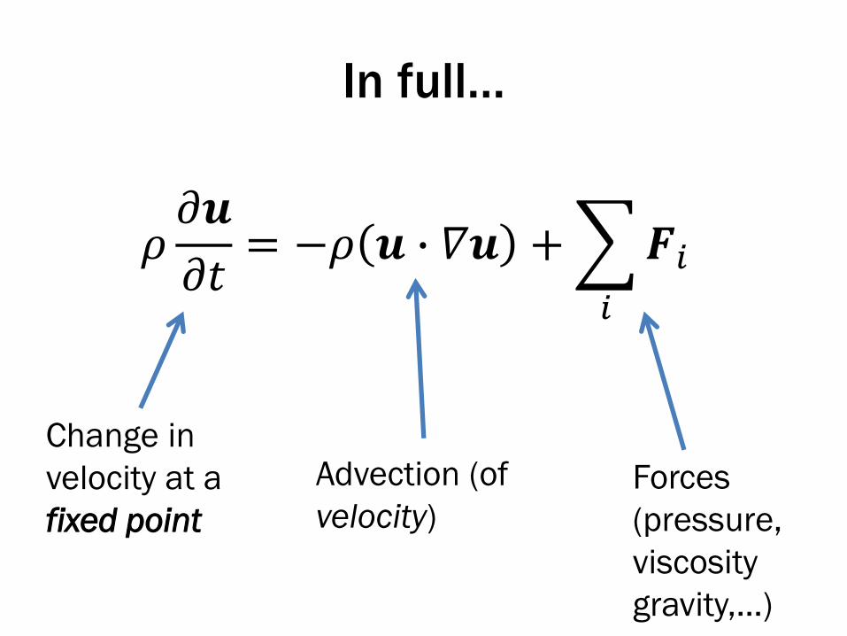
In full…
𝜌𝜕𝒖
𝜕𝑡= −𝜌 𝒖 ∙ 𝛻𝒖 +
𝑖
𝑭𝑖
Advection (of
velocity)
Change in
velocity at a
fixed point
Forces
(pressure,
viscosity
gravity,…)

Operator splitting
Break the full, nonlinear equation into sub-
steps:
1. Advection: 𝜌𝜕𝒖
𝜕𝑡= −𝜌 𝒖 ∙ 𝛻𝒖
2. Pressure: 𝜌𝜕𝒖
𝜕𝑡= 𝑭𝑝𝑟𝑒𝑠𝑠𝑢𝑟𝑒
3. Viscosity: 𝜌𝜕𝒖
𝜕𝑡= 𝑭𝑣𝑖𝑠𝑐𝑜𝑠𝑖𝑡𝑦
4. External: 𝜌𝜕𝒖
𝜕𝑡= 𝑭𝑜𝑡ℎ𝑒𝑟

1. Advection

Advection
Earlier, we considered advection of a passive scalar quantity, 𝑇, by velocity 𝒖.
In Navier-Stokes we saw:
Velocity 𝒖 is advected by itself!
𝜕𝒖
𝜕𝑡= −𝒖 ∙ 𝛻𝒖
𝜕𝑇
𝜕𝑡= −𝒖 ∙ 𝛻𝑇

Advection
That is, 𝑢, 𝑣, 𝑤 components of velocity 𝒖 are
advected as separate scalars.
May be able to reuse the same numerical
method.

2. Pressure
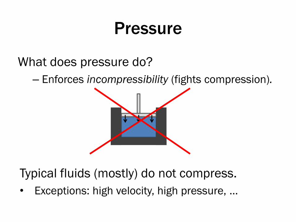
Pressure
What does pressure do?
– Enforces incompressibility (fights compression).
Typical fluids (mostly) do not compress.
• Exceptions: high velocity, high pressure, …
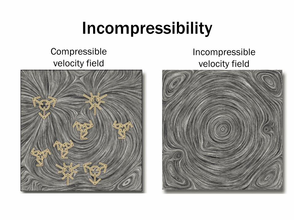
Incompressibility
Compressible
velocity field
Incompressible
velocity field

Incompressibility
Intuitively, net flow into/out of a given region is zero (no sinks/sources).
Integrate the flow across the boundary of a closed region:
𝜕Ω
𝒖 ∙ 𝒏 = 0
𝒏

Incompressibility
𝜕Ω
𝒖 ∙ 𝒏 = 0
By divergence theorem:
𝛁 ∙ 𝒖 = 0
But this is true for any region, so 𝛁 ∙ 𝒖 = 𝟎everywhere.
Incompressibility implies 𝒖 is divergence-free.
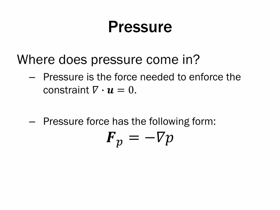
Pressure
Where does pressure come in?
– Pressure is the force needed to enforce the
constraint 𝛻 ∙ 𝒖 = 0.
– Pressure force has the following form:
𝑭𝑝 = −𝛻𝑝

Helmholtz Decomposition
= +
Input (Arbitrary)
Velocity Field
Curl-Free
(Irrotational)
Divergence-Free
(Incompressible)
𝑢 = 𝛻𝑝 + 𝛻 × 𝜑
𝑢𝑜𝑙𝑑 = 𝐹𝑝𝑟𝑒𝑠𝑠𝑢𝑟𝑒 + 𝑢𝑛𝑒𝑤

Aside: Pressure as Lagrange Multiplier
Interpret as an optimization:
Find the closest 𝒖𝑛𝑒𝑤 to 𝒖𝑜𝑙𝑑 where 𝛻 ∙ 𝒖𝑛𝑒𝑤 = 0
argmin𝒖𝑛𝑒𝑤
𝜌
2𝒖𝑛𝑒𝑤 − 𝒖𝑜𝑙𝑑
2
subject to 𝛻 ∙ 𝒖𝑛𝑒𝑤 = 0
The Lagrange multiplier that enforces the constraint is the pressure.e.g., recall the “fast projection” paper, Goldenthal et al. 2007.

3. Viscosity

High Speed Honey

Viscosity
What characterizes a viscous liquid?
• “Thick”, damped behaviour.
• Strong resistance to flow.

Viscosity
Loss of energy due to internal friction between molecules moving at different velocities.
Interactions between molecules causes shear stressthat…
• opposes relative motion.
• causes an exchange of momentum.

Viscosity
Loss of energy due to internal friction between molecules moving at different velocities.
Interactions between molecules causes shear stressthat…
• opposes relative motion.
• causes an exchange of momentum.

Viscosity
Loss of energy due to internal friction between molecules moving at different velocities.
Interactions between molecules causes shear stressthat…
• opposes relative motion.
• causes an exchange of momentum.

Viscosity
Loss of energy due to internal friction between molecules moving at different velocities.
Interactions between molecules causes shear stressthat…
• opposes relative motion.
• causes an exchange of momentum.

Viscosity
Imagine fluid particles with general velocities.
Each particle interacts with nearby neighbours, exchanging momentum.
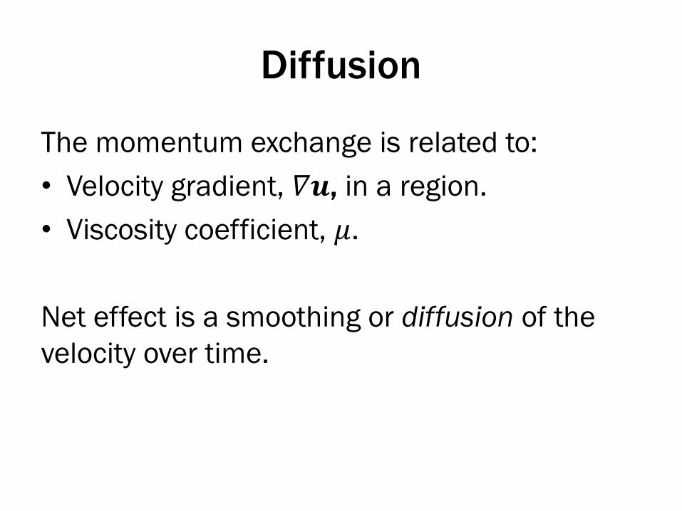
Diffusion
The momentum exchange is related to:
• Velocity gradient, 𝛻𝒖, in a region.
• Viscosity coefficient, 𝜇.
Net effect is a smoothing or diffusion of the
velocity over time.

Viscosity
Diffusion is typically modeled using the heat equation:𝑑𝑇
𝑑𝑡= 𝛼𝛁 ∙ 𝛁𝑇

Viscosity
Diffusion applied to velocity gives our viscous
force:
Usually, diffuse each component of 𝒖 =(u, v, w)
separately.
𝑭𝑣𝑖𝑠𝑐𝑜𝑠𝑖𝑡𝑦 = 𝜌𝜕𝒖
𝜕𝑡= 𝜇𝛁 ∙ 𝛁𝒖

4. External Forces

External Forces
Any other forces you may want.
• Simplest is gravity:
– 𝐹𝑔 = 𝜌𝒈 for 𝒈 = (0,−9.81, 0)
• Buoyancy models are similar,
– e.g., 𝐹𝑏 = 𝛽(𝑇𝑐𝑢𝑟𝑟𝑒𝑛𝑡 − 𝑇𝑟𝑒𝑓)𝒈

Numerical Methods for Fluid
Animation

1. Advection

Advection of a Scalar
Consider advecting a quantity, 𝜑
– temperature, color, smoke density, …
according to a velocity field 𝒖.
Allocate a grid (2D array) that
stores scalar 𝜑 and velocity 𝒖.

Eulerian
Approximate derivatives with finite differences.𝜕𝜑
𝜕𝑡+ 𝒖 ∙ 𝛻𝜑 = 0
FTCS = Forward Time, Centered Space:
𝜑𝑖𝑛+1 − 𝜑𝑖
𝑛
∆𝑡+ 𝑢𝜑𝑖+1
𝑛 − 𝜑𝑖−1𝑛
2∆𝑥= 0
Unconditionally
Unstable!
Conditionally
Stable!
Lax:
𝜑𝑖𝑛+1 − (𝜑𝑖+1
𝑛 + 𝜑𝑖−1𝑛)/2
∆𝑡+ 𝑢𝜑𝑖+1
𝑛 − 𝜑𝑖−1𝑛
2∆𝑥= 0
Many possible methods, stability can be a challenge.

Lagrangian
Advect data “forward” from grid points by integrating position according to grid velocity (e.g. forward Euler).
Problem: New data position doesn’t necessarily land on a grid point.
?

Semi-Lagrangian
• Look backwards in time from a grid point, to
see where its new data is coming from.
• Interpolate data at previous time.

Semi-Lagrangian - Details
1. Determine velocity 𝒖𝑖,𝑗 at grid point.
2. Integrate position for a timestep of −∆𝑡.
e.g. 𝑥𝑏𝑎𝑐𝑘 = 𝑥𝑖,𝑗 − ∆𝑡𝒖𝑖,𝑗
3. Interpolate 𝜑 at 𝑥𝑏𝑎𝑐𝑘, call it 𝜑𝑏𝑎𝑐𝑘.
4. Assign 𝜑𝑖,𝑗 = 𝜑𝑏𝑎𝑐𝑘 for the new time.
Unconditionally stable!(Though dissipative – drains energy over time.)

Advection of Velocity
This handles scalars. What about advecting velocity?
Same method:– Trace back with current velocity
– Interpolate velocity at that point
– Assign it to the grid point at the new time.
Caution: Do not overwrite the velocity field you’re using to trace back! (Make a copy.)
𝜕𝒖
𝜕𝑡= −𝒖 ∙ 𝛻𝒖

2. Pressure

Recall… Helmholtz Decomposition
= +
Input Velocity field Curl-Free
(irrotational)
Divergence-Free
(incompressible)
𝑢 = 𝛻𝑝 + 𝛻 × 𝜑
𝑢𝑜𝑙𝑑 = 𝐹𝑝𝑟𝑒𝑠𝑠𝑢𝑟𝑒 + 𝑢𝑛𝑒𝑤

Pressure Projection - Derivation
(1) 𝜌𝜕𝒖
𝜕𝑡= −𝛻𝑝 and (2) 𝛻 ∙ 𝒖 = 0
Discretize (1) in time…
𝒖𝑛𝑒𝑤 = 𝒖𝑜𝑙𝑑 −∆𝑡
𝜌𝛻𝑝
Then plug into (2)…
𝛻 ∙ 𝒖𝑜𝑙𝑑 −∆𝑡
𝜌𝛻𝑝 = 0

Pressure Projection
Implementation:
1) Solve a linear system of equations for p:∆𝑡
𝜌𝛻 ∙ 𝛻𝑝 = 𝛻 ∙ 𝒖𝑜𝑙𝑑
2) Given p, plug back in to update velocity:
𝒖𝑛𝑒𝑤 = 𝒖𝑜𝑙𝑑 −∆𝑡
𝜌𝛻𝑝

Implementation
Discretize with finite differences:
e.g., in 1D:
∆𝑡
𝜌
𝑝𝑖+1 − 𝑝𝑖∆𝑥
−𝑝𝑖 − 𝑝𝑖−1∆𝑥
∆𝑥=𝑢𝑖+1𝑜𝑙𝑑− 𝑢𝑖
𝑜𝑙𝑑
∆𝑥
𝑝𝑖+1 𝑝𝑖−1𝑝𝑖
𝑢𝑖+1 𝑢𝑖
∆𝑡
𝜌𝛻 ∙ 𝛻𝑝 = 𝛻 ∙ 𝒖𝑜𝑙𝑑

Solid Boundary Conditions
58
𝒏
𝒖
Free Slip:𝒖𝑛𝑒𝑤∙ 𝒏 = 0
i.e., Fluid cannot penetrate or
flow out of the wall, but may
slip along it.

Air (“Free surface”) Boundary
Conditions
Assume air (outside the liquid) is at some
constant atmospheric pressure, 𝑝 = 𝑝𝑎𝑡𝑚.

Free Surface Boundary Conditions
Only the pressure gradient matters, so simplify
and assume 𝑝 = 𝑝𝑎𝑡𝑚 = 0.
p=0
p=10
p=20
p=100
p=110
p=120
Same (vertical)
pressure
gradient, 𝛻𝑝.

3. Viscosity

Viscosity
PDE: 𝜌𝜕𝒖
𝜕𝑡= 𝜇𝛻 ∙ 𝛻𝒖
Again, apply finite differences.
Discretized in time:
𝒖𝒏𝒆𝒘 = 𝒖𝑜𝑙𝑑 +∆𝑡𝜇𝜌𝛻 ∙ 𝛻𝒖∗
𝒖𝒐𝒍𝒅 -> explicit
𝒖𝒏𝒆𝒘 -> implicit

Viscosity – Time Integration
Explicit integration:
– Compute ∆𝑡𝜇𝜌𝛻 ∙ 𝛻𝒖𝑜𝑙𝑑 from current velocities.
– Add on to current 𝒖.
– Quite unstable (stability restriction: ∆𝑡 ≈ 𝑂(∆𝑥2))
Implicit integration:
– Stable even for high viscosities, large steps.
– Must solve a system of equations.
𝒖𝒏𝒆𝒘 = 𝒖𝑜𝑙𝑑 +∆𝑡𝜇𝜌 𝛻 ∙ 𝛻𝒖𝑜𝑙𝑑
𝒖𝒏𝒆𝒘 = 𝒖𝑜𝑙𝑑 +∆𝑡𝜇𝜌 𝛻 ∙ 𝛻𝒖𝑛𝑒𝑤
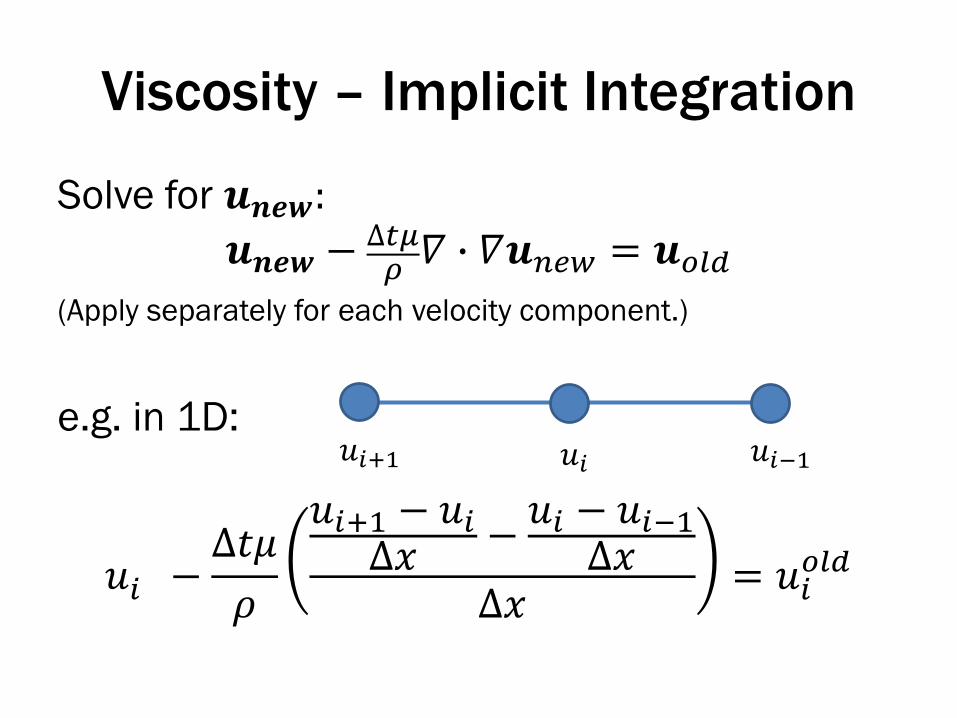
Viscosity – Implicit Integration
Solve for 𝒖𝒏𝒆𝒘:
𝒖𝒏𝒆𝒘 −∆𝑡𝜇𝜌𝛻 ∙ 𝛻𝒖𝑛𝑒𝑤 = 𝒖𝑜𝑙𝑑
(Apply separately for each velocity component.)
e.g. in 1D:
𝑢𝑖 −∆𝑡𝜇
𝜌
𝑢𝑖+1 − 𝑢𝑖∆𝑥
−𝑢𝑖 − 𝑢𝑖−1∆𝑥
∆𝑥= 𝑢𝑖𝑜𝑙𝑑
𝑢𝑖+1 𝑢𝑖−1𝑢𝑖

Viscosity - Solid Boundary Conditions
65
No-Slip:𝒖𝑛𝑒𝑤= 0

No-slip Condition

Viscosity - Free Surface Conditions
We want to model no momentum exchange with the “air”.
Simplest attempt: 𝛻𝑢 ∙ 𝑛 = 0
Drawback: Breaks rotation!
True conditions are more involved:
(Still ignores surface tension!)
See [Batty & Bridson, 2008] for the current standard solution in graphics. (Needed e.g., for honey coiling.)
−𝑝𝐈 + 𝛍 𝛁𝒖 + 𝛁𝒖𝑻 ∙ 𝒏 = 𝟎

4. External Forces
Gravity
Discretized form is:
𝒖𝒏𝒆𝒘 = 𝒖𝑜𝑙𝑑 + ∆𝑡𝒈
Simply increment the vertical velocities at
each step!

Gravity
Notice: in a closed fluid-filled container, gravity
(alone) won’t do anything!
– Incompressibility cancels it out. (Assuming constant density.)
Start After gravity step After pressure step

Simple Buoyancy
Track an extra scalar field T, representing local
temperature.
Apply advection and diffusion to evolve it with the
velocity field.
Difference between current and “reference”
temperature induces buoyancy.

Simple Buoyancy
e.g.
𝒖𝒏𝒆𝒘 = 𝒖𝑜𝑙𝑑 + ∆𝑡𝛽 𝑇𝑐𝑢𝑟𝑟𝑒𝑛𝑡 − 𝑇𝑟𝑒𝑓 𝒈
𝛽 dictates the strength of the buoyancy
force.
For an enhanced version of this:
“Visual simulation of smoke”, [Stam et al., 2001].
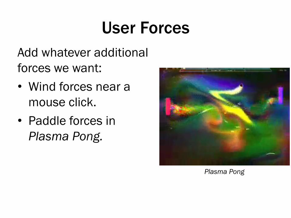
User Forces
Add whatever additional
forces we want:
• Wind forces near a
mouse click.
• Paddle forces in
Plasma Pong.
Plasma Pong

Ordering of Steps
Order is important.
Why?
1) Incompressibility is not satisfied at
intermediate steps.
2) Advecting with a compressive field causes
volume/material loss or gain!

Ordering of Steps
For example, consider advection in this field:

The Big Picture
Velocity Solver
Advect Velocities
Add Viscosity
Add Gravity
Project Velocities
to be
Incompressible
Liquids

Liquids
What’s missing?
We still need a surface representation.

Interaction between
Solver and Surface Tracker
Advect Velocities
Add Viscosity
Add Gravity
Project Velocities
to be
Incompressible
Surface Tracker
Velocity Solver
Velocity
Information
Geometric
Information
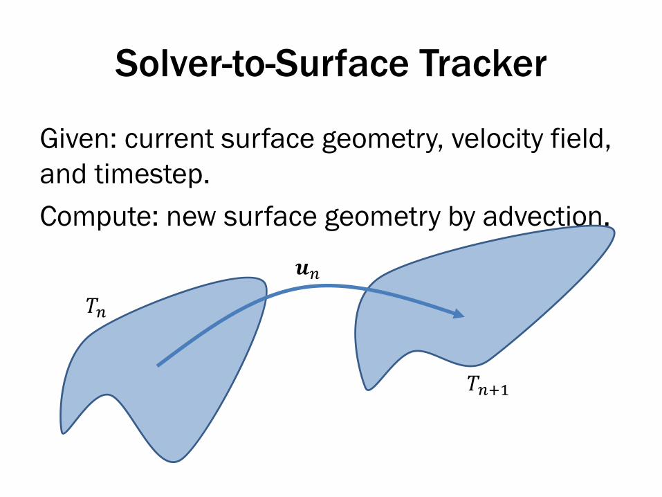
Solver-to-Surface Tracker
Given: current surface geometry, velocity field,
and timestep.
Compute: new surface geometry by advection.
𝑇𝑛
𝑇𝑛+1
𝒖𝑛

Surface Tracker-to-Solver
Given the surface geometry, identify the type of each cell.
Solver uses this information for boundary conditions.
S
S
S
S
S
S S S S
S
S
S
L L
L L
L
A A A

Surface Tracker
Ideally:
• Efficient
• Accurate
• Handles merging/splitting (topology changes)
• Conserves volume
• Retains small features
• Gives a smooth surface for rendering
• Provides convenient geometric operations (post-processing?)
• Easy to implement…
Very hard (impossible?) to do all of these at once.

Surface Tracking Options
1. Particles
2. Level sets
3. Volume-of-fluid (VOF)
4. Triangle meshes
5. Hybrids (many of these)

Particles
[Zhu & Bridson 2005]

Particles
Perform passive Lagrangian advection on each
particle.
For rendering, need to reconstruct a surface.

Level sets
[Losasso et al.
2004]

Level setsEach grid point stores signed distance to the
surface (inside <= 0, outside > 0).
Surface is the interpolated zero isocontour.
> 0
<= 0

Densities / Volume of fluid
[Mullen et al 2007]
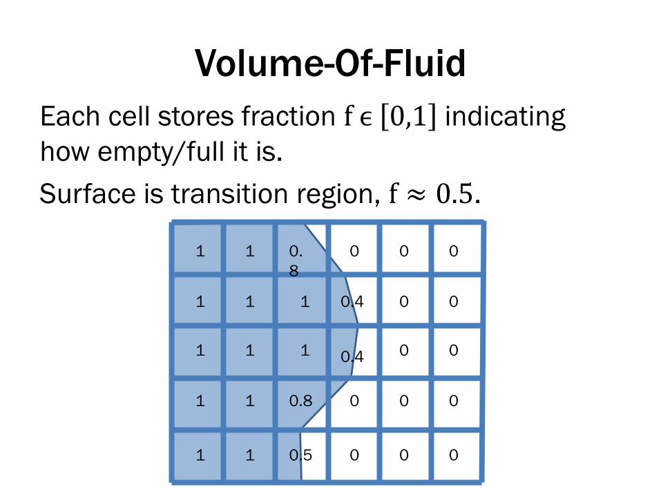
Volume-Of-Fluid
Each cell stores fraction f ϵ 0,1 indicating
how empty/full it is.
Surface is transition region, f ≈ 0.5.
0
0
0
0
0
0
0
0
0
0
0
0.4
0.4
0
0
0.
8
1
1
0.8
0.5
1
1
1
1
1
1
1
1
1
1

Meshes
[Brochu et al 2010]

Meshes
Store a triangle mesh.
Advect its vertices, and deal with collisions.


![ABSTRACT arXiv:1608.03983v2 [cs.LG] 17 Aug 2016 · PDF fileSGDR: STOCHASTIC GRADIENT DESCENT WITH RESTARTS ... Powell (1977) proposed to ... i.e, when the momentum seems to be taking](https://static.fdocuments.us/doc/165x107/5aa32f827f8b9a46238e09ea/abstract-arxiv160803983v2-cslg-17-aug-2016-stochastic-gradient-descent-with.jpg)