An Optimum Hierarchical Sampling Procedure for Cross-Bedding DataAuthor(s): J. S. Rao and Supriya SenguptaSource: The Journal of Geology, Vol. 78, No. 5 (Sep., 1970), pp. 533-544Published by: The University of Chicago PressStable URL: http://www.jstor.org/stable/30061390Accessed: 30/09/2010 17:49

Your use of the JSTOR archive indicates your acceptance of JSTOR's Terms and Conditions of Use, available athttp://www.jstor.org/page/info/about/policies/terms.jsp. JSTOR's Terms and Conditions of Use provides, in part, that unlessyou have obtained prior permission, you may not download an entire issue of a journal or multiple copies of articles, and youmay use content in the JSTOR archive only for your personal, non-commercial use.

Please contact the publisher regarding any further use of this work. Publisher contact information may be obtained athttp://www.jstor.org/action/showPublisher?publisherCode=ucpress.

Each copy of any part of a JSTOR transmission must contain the same copyright notice that appears on the screen or printedpage of such transmission.

JSTOR is a not-for-profit service that helps scholars, researchers, and students discover, use, and build upon a wide range ofcontent in a trusted digital archive. We use information technology and tools to increase productivity and facilitate new formsof scholarship. For more information about JSTOR, please contact support@jstor.org.

The University of Chicago Press is collaborating with JSTOR to digitize, preserve and extend access to TheJournal of Geology.

http://www.jstor.org

AN OPTIMUM HIERARCHICAL SAMPLING PROCEDURE

FOR CROSS-BEDDING DATA1

J. S. RAO2 AND SUPRIYA SENGUPTA

Indian Statistical Institute, Calcutta-35, India

ABSTRACT The commonly used techniques for hierarchical or multistage sampling of cross-bedding foreset azimuths

(for paleocurrent study) are based on the conventional analysis of variance. It is now well known that the classical method of analysis of variance (ANOVA), which partitions the sum of squares of the observations, can not be indiscriminately applied for the analysis of circularly distributed directional data. An efficient and economical sampling technique for cross-bedding data has been developed using the circular measures of dispersion and the approximate ANOVA of Watson. The technique is illustrated here with the help of the pilot-survey data of the fluviatile Kamthi formation. The following sampling problems have been solved: (1) the minimum sample size required for estimating, with a desired precision, the mean direction of a for- mation, (2) the optimum allocation of the samples between and within the outcrops that would allow effi- cient sampling at minimum cost.

INTRODUCTION

Cross-bedding foreset dip directions are known to provide one of the most depend- able clues to the paleocurrent. For efficient and economical sampling of foreset dip di- rections in a profusely cross-bedded forma- tion, it is essential to know the minimum number of observations which would give a mean direction with specified precision for the whole formation.

An early attempt to provide a suitable, single stage sampling plan for cross-bedding was made by Reiche (1938) who suggested the technique of determination of the "flat- ness point" in a curve of the "cumulative vector directions" plotted against the num- ber of measurements. At a later date, Potter and Olson (Potter and Olson 1954; Olson and Potter 1954) following a hierarchical sampling plan, measured the variability as- sociated with different levels of sampling (between areas, between outcrops, between beds, and within beds). Their observations in the Pennsylvanian Mansfield formation showed largest variation between outcrops

1 Manuscript received December 12, 1969; re- vised February 18, 1970.

2 Present address: Department of Mathematics, Indiana University, Bloomington, Indiana 47401.

[JOURNAL OF GEOLOGY, 1970, Vol. 78, p. 533-544]

@ 1970. The University of Chicago. All rights reserved.

within townships and least variation within cross-bedded units. Potter and Pettijohn (1963) have also recommended the analysis of variance (ANOVA) for development of an efficient sampling plan.

Raup and Miesch (1957) have suggested a simple field method for determination of the most efficient and economical sampling scheme. Their method is based on Stein's two-stage sampling procedure where the minimum number of measurements required to obtain a "significant average" (an aver- age which lies within previously specified confidence limits) is estimated from the standard deviation of the first fifty measure- ments.

It has been stressed by a number of ear- lier authors (e.g., Watson 1966; Sengupta and Rao 1966; Rao 1969) that the conven- tional statistical techniques are of little use in the analysis of circularly distributed di- rectional data like cross-bedding foreset azimuths. Although the directions can be measured as angles with respect to some arbitrary origin, the arithmetic mean fails to provide a representative measure of the mean for such data, and the usual standard deviation of measurements) using the approximate ANOVA of Watson (1956, method of ANOVA, which partitions the sums of squares of the observations, can not be indiscriminately applied in the analysis

533

J. S. RAO AND SUPRIYA SENGUPTA

of circularly distributed directional data. These facts put into doubt the sampling plans of the earlier authors (e.g., Potter and Olson 1954; Potter and Pettijohn 1963; Raup and Miesch 1957) which were based on the conventional ANOVA.

It is now well known that the direction of sample resultant provides a reasonable estimate of the population mean direction for data having unimodal circular distribu- tion, and the length of the resultant can be used to obtain an appropriate measure of dispersion. The purpose of the present paper is to develop an efficient sampling technique which takes into consideration the circular measures of dispersion (instead of the usual standard deviation of measurements) using the approximate ANOVA of Watson (1956, 1966). Admittedly, the methods adopted here are approximate, but these approxima- tions can be shown to hold good with a fair degree of accuracy.

Attempts will be made to answer three major questions in the present paper: (1) how many observations should be taken within a geological formation so that the mean direction is reasonably close to the true value of the mean, (2) how should the sampling effort be distributed over two stages (between outcrops and within out- crops) so that the overall estimate has the desired precision, and (3) if cost (or time) considerations could be profitably intro- duced, what is the procedure which would minimize the cost (or time) involved. The questions posed here are the usual questions faced in sampling and have been handled in several standard texts on the subject. The novelty of the present approach lies essen- tially in the use of the circular measures of dispersion and the corresponding ANOVA instead of the classical ANOVA based on variances.

GEOLOGY OF THE AREA AND THE PILOT SURVEY

The technique of analysis developed here is illustrated with the help of the data ob- tained from the Permo-Triassic, fluvial Kam- thi formation. Three members of the Kamthi (lower, middle, and upper) were sampled

near Bheemaram, in southeast India for this purpose. Depositional environments of these rocks have been discussed in detail elsewhere (Sengupta 1970). In short, the upper and the middle Kamthi sandstones represent the younger and older point-bar and channel- bar deposits of the Kamthi river. A part of the middle Kamthi member also includes the levee deposits adjacent to the main river channel. The lower Kamthi sandstones represent cutoff meander channels within the older floodplain deposits of the river. An earlier statistical analysis of a large sample of the Kamthi data has indicated that the population means of the cross-beddings as well as their dispersions are significantly dif- ferent in the three Kamthi members (Sen- gupta and Rao 1966).

For the purpose of the present work, a "pilot survey" was conducted and a set of 280 fresh measurements were taken in about 42 square miles of the Kamthi formation, following a rigid sampling scheme. A mini- mum number of widely spaced outcrops were measured from the three Kamthi mem- bers. Although the choice of an outcrop was partly guided by its accessibility, this was not allowed to be a significant source of bias in the analysis. The number of outcrops measured in each case was broadly propor- tional to the exposed area of the Kamthi member concerned. Thus, six outcrops were measured from the lower Kamthi member (area: approximately 8 square miles), eight from the middle Kamthi member (area: ap- proximately 12 square miles), and fourteen from the upper Kamthi member (area: ap- proximately 22 square miles). A fixed num- ber of ten measurements of foreset-dip direc- tions were made in each outcrop by random sampling.

The model and method of analysis de- scribed below give a general idea of the sampling plan to be adopted under two dis- tinctly different conditions: (1) when the cross-beddings are profuse and the foreset- dip directions are fairly consistent, as in the middle and the upper Kamthi, and (2) when the cross-beddings are less frequent and the dispersions are relatively higher, as in the lower Kamthi.

534

SAMPLING PROCEDURE FOR CROSS-BEDDING DATA

The method of analysis discussed here (and illustrated with the Kamthi data) is of a general nature and can be utilized by anyone having similar problems involving circular data.

THE MODEL AND THE METHOD

OF ANALYSIS

We will consider a hierarchical or multi- stage sampling scheme. For our purposes it is sufficient to consider a situation with only two levels, though the results of this and the next section can easily be extended to the case where there are more levels of classification. Suppose, as in the present case, the first-stage units are called "out- crops" and the second-stage units, "observa- tions." Further, suppose that we have taken n first-stage units or outcrops and m second- stage units or observations from each of these first-stage units. It is, however, not essential to choose the same number of sec- ond-stage units from each first-stage unit though this will considerably simplify the computations as well as the expressions in- volved. Let cij denote the jth observation from the ith outcrop (j = 1, ... m; i = 1, .. ., n) of the formation. We assume

#is = 7 + (4 + €~ , (1)

where 7 = the mean direction for the for- mation, (i = deviation due to the ith out- crop from the overall (or formation) mean direction, and ei = error term. The devia- tions at each level are supposed to average out to the mean of the next higher level. For example, if the number of observations are increased indefinitely in an outcrop, then their resultant direction would approach the particular outcrop mean direction. More precisely, we assume that within the ith outcrop, the observations 4i, have a "circu- lar normal distribution" (CND), with mean direction (7 + (i) and a concentration parameter 0w. It may be recalled that a ran- dom angle 4, with reference to any arbi- trary vector in two dimensions, is said to have a CND with parameters y and K if it has the density

1 e" (-<>, O < 4 < 2r. (2)

Here 7 is the population-mean angle and K is a measure of concentration, larger values of K standing for more concentration around the mean direction 7. While 4,i's for any fixed i have a CND with parameters 7 + (, and w, the (,'s themselves have a CND with the mean direction as the zero direction and a concentration parameter, fp. In other words, the different outcrop means have a CND whose mean is the formation mean y and whose concentration parameter is 3. It

may be remarked that most of our analysis would remain valid even if the assumptions of circular normality do not hold strictly for the data in question.

In a particular formation in whose mean direction we are interested, suppose we visit- ed n outcrops and took m observations from each of them, thus making a total sample of size N = mn for the whole forniation. We then compute the lengths of the resultant Ri(i = 1, . . . , n) where

R: = cos < + ( sin <~ i (3)

for the n individual outcrops as well as the length of the overall resultant, R, where

R2 = cos i2 i=1 j=1 I

+ sin $ij <= 1

(4)

based on all the N observations. Now it is well known (Watson 1966; Rao 1969) that if R is the length of the resultant based on p observations from a CND with concentra- tion parameter K, then 2K(p - R) is ap- proximately distributed as a x2 with (p - 1) degrees of freedom if K is large. Using this fact, one can have the following approxi- mate ANOVA for the angular data (Watson 1966). Here

n

1 1 m n - 1 N (5)

in case a variable number of mi observations are taken from the ith outcrop. This mf is a

535

J. S. RAO AND SUPRIYA SENGUPTA

weighted average of the mi's, and if mi = m for all outcrops then ii = m.

From table 1 we can test the significance of between-outcrop variations by using the F-test

which has a F distribution with (n - 1) and (N - n) degrees of freedom under the usual ANOVA set up or under the so-called Model I of ANOVA. Under Model II, the same technique and computations may be used to estimate the between-outcrop and

again have a CND with a concentration parameter

(7) 1 + (n )-' + (N~)-1

These results for the circular (or two- dimensional) data are completely analogous to those of Watson (1966) and Watson and Irving (1957) for the three-dimensional di- rections.

ESTIMATING THE FORMATION-MEAN DIRECTION WITH A SPECIFIED

PRECISION

Suppose we want to estimate the forma- tion mean 7 with a semiangle of confidence

TABLE 1

ANOVA TABLE FOR ANGULAR DATA

Source of Variation df SS MS E(MS) (1) (2) (3) (4) (5)

Between outcrops n-1 R-R (,Ri-R)/(n- 1) a)

^1 Within outcrops N-n N- _R (N- ZRi)/(N-n)

Total N-1 N-R

within-outcrop concentrations-0 and co, re- spectively-under the assumptions we have made in the beginning of this section. If the test in (6) shows no significant variation be- tween the sites (or outcrops), then the be- tween-outcrop variation may be ignored or, in other words, the concentration parameter B may be taken to be infinity. If, on the other hand, the F-test gives a significant re- sult, then the estimates of f and w, say f and co, may be obtained by equating the mean squares (MS) in column 4 of table 1 with the corresponding expectations in col- umn 5.

Now if all the N = mn observations are used to get the overall resultant and its di- rection iN is used to estimate the mean direction of the formation, then this will

,lo at a confidence level 1 - a, (0 < a < 1). That is, if VN denotes the direction of the overall resultant based on N observations, we want the estimate 7N to lie within the interval 7 - /o to 7 + Lo in (1 - a) per- cent of the cases. This would clearly depend on the distribution of TN, which from the earlier section is circular normal with con- centration given by (7). Thus the concen- tration parameter K associated with the dis- tribution of iN would determine the con- fidence interval for 7. But since in our case the problem is one of finding the sample size required in order to have a confidence interval of specified width and confidence level, we try to determine a value of K, say KO, required for 7j to lie in the specified in- terval with the given probability. Thus we

536

F

(6)

SAMPLING PROCEDURE FOR CROSS-BEDDING DATA

must first answer the question: How large should K be such that a semiangle of confi- dence #o around y carries a probability of (1 - a) percent? If K were less than 7, one can refer to Watson's (1966) chart and read out the required K. But this range of K values is too small to be of use in most practical situations of our interest where the K values often exceed 100. For such large values of K, the following normal approximation to the CND can profitably be used. If 4 is a ran- dom angle having a CND with parameters 7 and K, then it is known that the distribu-

standard normal distribution (e.g., Xa = 1.96 for a = 5 percent). Comparing (8) and (9), VKo #o = Xa or

Xe KO = Po

We give a short table of values of Ko (table 2) required to attain some commonly specified precisions as given by /o and a.

Thus if tN is to attain the given precision, the number of outcrops n and the number of observations in each, namely, m, should

TABLE 2

VALUE OF Ko REQUIRED FOR YN TO

ATTAIN A GIVEN PRECISION

fo (1-a) KO Semiangle of Confi- Confidence Concentration

dence Level Value Required

50 0.90 354.6292 0.95 504.0610 0.99 870.6882

100 0.90 88.7598 0.95 126.1125 0.99 217.9236

200 0.90 22.1772 0.95 31.5221 0.99 54.4496

tion of 4* = /K (4 - y) approaches a standard normal distribution for large K. Therefore, for given a(0 < a < 1), we want a K for which

(1 - a) = P, (7 - to < 7 + 0o)

- P(-V/ Ko < V (qS- y)

(8) < V/ ro)

= P(1*1 <V ' o).

But since 4* is distributed as N(0, 1), we have

P(| ** < xi) = (1 - )o (9)

where X, is the a percent point for the

be such as to give a K value as shown in table 2. In other words, from (7) m and n should be such as to satisfy the equation

1

o (KO )_, + (m )-1 " (11)

in order that the overall resultant direction

have a specified accuracy, where Ko is de- termined by #ko and a and is obtained from table 2. The equation (11) still does not com- pletely specify what m and n should be.

Several sets of m and n values are possible, of which we may choose one depending on the convenience and availability of out- crops. For example, if a maximum number

537

(10)

J. S. RAO AND SUPRIYA SENGUPTA

of only no outcrops are available, then one can obtain the value of m from (11) as

1 m = (.l--- -

If, on the other hand, a large number of out- crops are available and one wants to take only one observation per outcrop (i.e., m = 1), then we need to visit

1 1 1\ n = - + -J

outcrops. Between these two extremes, one has several choices for m and n, all of which lead to the same precision for the overall resultant direction.

We will now introduce cost considera- tions into the picture and then try to ar- rive at an optimum choice of m and n, that is, a choice which minimizes the total cost of the operation. We generally have a rough idea as to the cost (or time) involved in visiting an outcrop and in taking a single observation. Let C1 be the cost involved in reaching the outcrop (location, identifica- tion, and transportation costs) and C2 be the cost of making an observation within the outcrop. Then the total cost involved in the operation may be expressed as

C = Co + nC1 + nmC2, (12)

where Co is the total overhead cost. Now we might ask for a choice of m and n, which, besides assuring us of a specified precision, minimizes the cost involved in the entire operation. It may be remarked that we do not need to have a precise idea about the costs C1 and C2. What is needed for our purposes is only a rough idea about the rela- tive costs, or the ratio Ci/C2.

It is clear from (7) that the number of outcrops, n, way be expressed as

n = Ko 6+ .• (13)

Substituting this in the cost function (12), we have

C = Co + n(Ci + mC2)

= Co + Ko(\ + ) (C1 + mC2)

(14) = terms not containing m

( Cx mC,\ + K + --) ,

which when minimized with respect to m gives

or m = (15)

Thus the optimum number of observations that should be taken from each outcrop is given by (15). Substituting this in (13), we get the corresponding value of n, the opti- mum number of outcrops. If m and n are chosen this way, the minimum cost asso- ciated with this operation (or survey) would be

Cmin = Co + KO (1+

• -C (16)

The optimum value of m given in (15) can also be found graphically by plotting the cost (14) as a function of m. Such graphs can be made for several choices of C1/C2 and /^/.

The expressions for the optimum values of m and n, say m* and n*, would, in gen- eral, contain a fractional part, in which case it may be rounded off to the next higher in- teger so that the final estimate would be at least as accurate as required. In fact, if this is done and, say, mo and no are the op- timum values so arrived at, then 'N will have a precision parameter

1 K (not)_ + (monoc)_ (17)

538

z cls m C2iL) )

SAMPLING PROCEDURE FOR CROSS-BEDDING DATA

and hence the semiangle of confidence for YN will be

= . (18)

We illustrate these ideas and methods in the following section by applying them to a specific situation.

ANALYSIS OF KAMTHI POPULATIONS

Earlier studies (Sengupta and Rao 1966) have shown that the cross-bedding foreset- dip directions of the three Kamthi members belong to three significantly different popu- lations. Thus we have a simple hierarchical

classification within each Kamthi member with two levels of sampling in each, namely, outcrops and observations.

As mentioned in the beginning, for the present analysis a total of twenty-eight out- crops were sampled, out of which fourteen are from the upper Kamthi (UK), eight from the middle Kamthi (MK), and the rest from the lower Kamthi (LK). From each outcrop we have taken a total of ten obser- vations at random though, as we remarked earlier, it is not essential to have the same number of observations within each outcrop. However this will facilitate computations.

We shall first deal with the UK, and the analysis of the other two populations pro- ceeds on exactly similar lines. We shall use the subscript U to denote the quantities corresponding to the UK population. We then have nv = 14 outcrops with my = 10

observations from each. The ANOVA table for these Nu = 140 observations belonging to the UK is given below. The data and the details of computation are not presented for reasons of brevity. The overall resultant based on all the 140 observations is Ru = (82.5159, -22.5615), with a length Ru = x/(82.5159)2 + (-22.5615)2 = 85.5447. The sum of the lengths of individual resultants is

14

Rwu = 91.8074. i=-1

From this, we form the ANOVA table for the UK data (see table 3). The value of the F-statistic, 1.2593, is insignificant at the 5

percent level with 13 and 126 degrees of freedom, the tabulated critical value being 1.83.3 Thus the variation between outcrops is not significant in the UK population and hence i, the measure of concentration be- tween UK outcrop means, may be taken to be infinity. In other words, all the UK out- crops may be taken to have the same mean direction which is also the UK formation- mean direction. If /3 = o, then estimate of w, say c&r, may be obtained by pooling the between and within the sum of the squares and the degrees of freedom. This gives cg = 2.5526.

Also equation (7) for K reduces to

K = NW . (19)

Therefore, the number of observations N * This situation needs special treatment not dis-

cussed earlier.

Source

Between outcrops

Within outcrops

Total

df

13

126

139

TABLE 3

ANOVA TABLE FOR UK DATA

SS MS

6.2627 0.4817

48.1926 0.3825

54.4553

E(MS)

1(1 10\ 2\wu +' 3u

1 2wv

F

F=1.2593

539

J. S. RAO AND SUPRIYA SENGUPTA

which one should take in order to attain a semiangle of say 100 with 95 percent confi- dence (which corresponds to a value of KO = 126.1125 from table 2) is

Ko 126.1125 N = 2.5526 49.40, (20)

U

or roughly fifty observations. Thus, in the UK, one can estimate the formation-mean direction to within +100 with 95 percent confidence on the basis of fifty observations.

However, the evidence for accepting the hypothesis / = oo is not strong, the F-value being not too small. Therefore, one may take into account the between-outcrop vari- ation also, in which case we follow the pro- cedure as outlined in the earlier section. We find the estimates, f and c, by equating col- umns 4 and 5 of table 3, and we get

Wu = 1.3072 and vu = 50.4032 (21)

for the UK formation. If we now wish to estimate the formation mean with + 100 ac- curacy with 95 percent confidence (which corresponds to a K value of 126.1125), the values m and n should satisfy the equation (7), that is,

126.1125 = nu ,

or (22) nv = 126.1125 [(50.4032)-1

+ (mu 1.3072)-1].

Throughout our present study we assume a cost ratio of Ci/C2 = 10/1, which seems to be reasonable in our case. Now appeal- ing to (15), the optimum number of obser- vations, say m*, to be taken within each UK outcrop is given by

= < CaC - 110 X 50.4032 m C2 ~ 1 X 1.3072 (23)

= 19.6,

or roughly twenty observations from each outcrop. Substituting this value of m*j = 20 in (22),

* 126.1125(5 1O) n 1 50.4032 + 26.1440/ (24)

= 7.3258,

or roughly 7.4 Thus in UK if one takes seven outcrops and twenty observations from each, this would, besides giving us the required accuracy, also minimize the overall cost of estimating the forma- tion mean. In fact, if we took seven out- crops and twenty observations from each, the accuracy parameter K for the overall resultant direction is, from (17), KU = 7/ {(50.4032)-' + [20(1.3072)]-1} = 120.5033, and hence the estimated mean direction has the semiangle of confidence

Xo.os 1.96 u VKU- V120.5033

= 0.1785 radians, (25)

or 100 13' with 95 percent confidence. Similar analysis can be done for the other

two Kamthi populations. For the eight out- crops of the MK with ten observations from each; we have ANOVA table 4. For 7 and 72 df, the F-value of 4.5660 is quite signifi- cant even at 1 percent level, the tabulated value being 2.14, and therefore the several site (outcrop) means differ significantly in the MK. Our model is thus more appropri- ate in this situation. Equating columns 4 and 5 of table 4, we get the estimates / and

for the MK, namely,

WM = 2.0000, and d/M = 5.6085. (26)

Now if we are to estimate the overall mean direction with a semiangle of ± 100 with 95 percent confidence as in the earlier case, the nM and mM should satisfy the equation

126.1125 = nM ()-1 + (mM .M)-1

or

nuM = 126.1125 [(5.6085)-1

+ (mM 2.0000)-1.

(27)

4 Earlier we suggested rounding off such fractions to the next higher integer. But this need not be fol-

540

SAMPLING PROCEDURE FOR CROSS-BEDDING DATA

But from equation (16) and an assumed cost ratio of 10/1, the optimum number of observations to be taken in a MK outcrop is

/10 X 5.6085 m = 1X 2.0000 = 5.295, (28)

or roughly 6. Now from (27) the number of outcrops to be visited in the MK is

n* = 126.1125 12000 (29) M 5.6085 12.0000 (29)

= 32.99,

or roughly 33. Thus for minimizing the cost of the operation, we need to take thirty-

Finally for the six outcrops of the LK, where again we have taken ten observations in each, we have the ANOVA shown in table 5. Here again the F-value is significant at 5 percent level with 5 and 54 df, the tabu- lated value being 2.40. Thus the site (out- crop) means in LK do vary significantly. Therefore, equating columns 4 and 5 of table 5, we have

<oL = 1.3154, and 1L = 6.1058. (31)

If we wish to estimate the LK formation mean by means of the direction of the over- all resultant, again with an accuracy of

TABLE 4

ANOVA TABLE FOR MK DATA

Source df SS MS E(MS) F

Between outcrops 7 7.9907 1.1415 - F=4.5660

Within outcrops 72 17.9985 0.2500 2M

Total 79 25.982

three outcrops in the MK but only six ob- servations from each. This larger number of outcrops is a consequence of the fact that in MK the between-outcrop varia- tion is very significant. This scheme of visit- ing thirty-three outcrops and taking six observations from each would give an ac- curacy parameter of KM = 33/[(5.6085)-1 + (6 X 2.0000)-1] = 126.1303 for the resul- tant based on 33 X 6 = 198 MK observa- tions. The MK mean can be estimated with a semiangle of

S 1.96

M = 126.1303 (30)

= 0.1745 radians,

or 100 with 95 percent confidence.

lowed as a hard and fast rule since that would often increase the sample size and we would have much more precision than we asked for.

+ 100 with 95 percent confidence, then the nL and mL should satisfy the equation

126.1125 = n ( L)-1 + (mLL)-1

or

nL = 126.1125 [(6.1058)-1 (32)

+ (mL 1.3154)-1].

But the equation (16) involving costs tells us that

S= O/10X 6.1058 m*I 1 X 1.3154 =6.8125, (33)

or roughly seven observations should be taken from each LK outcrop. Substituting this value of mL = 7 in (32),

,* = 126.1125[ 1 1 =121 6.1058 7(1.3154)

= 34.35 ,

541

J. S. RAO AND SUPRIYA SENGUPTA

or roughly 34. Thus we should sample thirty-four outcrops in the LK taking seven observations from each which leads to an accuracy parameter of

34 K"= (6.1058)-i + [7(1.3154)]-1

= 124.8246

for the distribution of the overall resultant direction. Then this sample mean direction based on 34 X 7 = 238 observations would be within PL = 1.96//124.8246 = 0.1754 radians, or 10°3' of the true LK formation mean with 95 percent confidence.

ber of observations required for estimation, with a desired precision, of mean direction which will be reasonably close to the true value of the formation mean; and (2) the pattern of distribution of the samples be- tween and within the outcrops that would allow sampling with optimum efficiency and at minimum cost.

The techniques used here in finding an- swers to these questions can be summarized as follows:

1. To start with, a small number of repre- sentative cross-bedding samples are ob- tained (a more or less uniformly spaced grid sample) for the population (formation) un-

TABLE 5

ANOVA TABLE FOR LK DATA

Source df SS MS E(MS) F

Between outcrops 5 5.9950 1.1990 + F=--3.1544

Within outcrops 54 20.5235 0.3801 2W.

Total 59 26.5185

SUM.MARY AND CONCLUSIONS

The techniques so far used for sampling and analysis of cross-bedding data were based on the conventional ANOVA. It is now well known that for the circularly dis- tributed directional data (like cross-bedding foreset azimuths) the technique of ANOVA is of little use. For such data, the direction of the sample resultant (instead of the arithmetic mean) provides a reasonable esti- mate of the population mean, and the length of the resultant (instead of the standard de- viation) provides an approximate measure of dispersion.

An efficient and economical sampling technique for cross-bedding directions has been developed in the present work using the circular measures of dispersion. With the help of the pilot-survey data of the flu- viatile Kamthi formation, it has been at- tempted to find out: (1) the minimum num-

der study. Observations from each outcrop within the population are recorded separate- ly. Equal number of observations from each outcrop facilitates computations, although this is not an essential requirement.

2. Sine and cosine values are computed for each foreset-dip direction (0) measured. The resultant direction for each outcrop is computed as in equation (3), that is,

R. = cos <) + E sin 0,)

= Co + s,

where Ri is the outcrop resultant for the ith outcrop and m = number of observations within each outcrop.

3. The overall resultant for all the out- crops is now computed as in (4), that is,

= i=l / + i

542

SAMPLING PROCEDURE FOR CROSS-BEDDING DATA

where n = number of outcrops surveyed and C and Si are as in step 2 above, that is,

Ci = E cos 4,i, and i-1

Si = C sin 4ii. i-1

4. The appropriate values are now filled in table 1.

5. The values for concentration within outcrop (co) and concentration between out- crops (B) are obtained by equating columns 4 and 5 of table 1.

6. The optimum number of observations

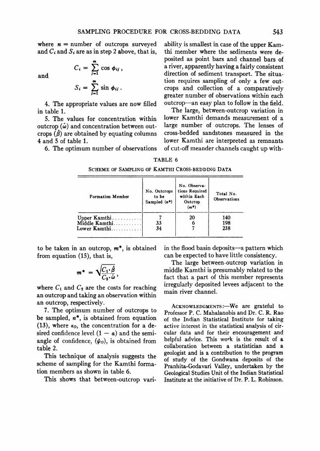
ability is smallest in case of the upper Kam- thi member where the sediments were de- posited as point bars and channel bars of a river, apparently having a fairly consistent direction of sediment transport. The situa- tion requires sampling of only a few out- crops and collection of a comparatively greater number of observations within each outcrop-an easy plan to follow in the field.

The large, between-outcrop variation in lower Kamthi demands measurement of a large number of outcrops. The lenses of cross-bedded sandstones measured in the lower Kamthi are interpreted as remnants of cut-off meander channels caught up with-

TABLE 6

SCHEME OF SAMPLING OF KAMTHI CROSS-BEDDING DATA

No. Observa- No. Outcrops tions Required Total No

Formation Member to be within Each Observations Sampled (n*) Outcrop

(m*)

Upper Kamthi 7 20 140 Middle Kamthi 33 6 198 Lower Kamthi 34 7 238

to be taken in an outcrop, m*, is obtained from equation (15), that is,

m* = C*^lf3 C2<0 '

where C1 and C2 are the costs for reaching an outcrop and taking an observation within an outcrop, respectively.

7. The optimum number of outcrops to be sampled, n*, is obtained from equation (13), where Ko, the concentration for a de- sired confidence level (1 - a) and the semi- angle of confidence, (/o), is obtained from table 2.

This technique of analysis suggests the scheme of sampling for the Kamthi forma- tion members as shown in table 6.

This shows that between-outcrop vari-

in the flood basin deposits-a pattern which can be expected to have little consistency.

The large between-outcrop variation in middle Kamthi is presumably related to the fact that a part of this member represents irregularly deposited levees adjacent to the main river channel.

ACKNOWLEDGMENTS:-We are grateful to Professor P. C. Mahalanobis and Dr. C. R. Rao of the Indian Statistical Institute for taking active interest in the statistical analysis of cir- cular data and for their encouragement and helpful advice. This work is the result of a collaboration between a statistician and a geologist and is a contribution to the program of study of the Gondwana deposits of the Pranhita-Godavari Valley, undertaken by the Geological Studies Unit of the Indian Statistical Institute at the initiative of Dr. P. L. Robinson.

543

J. S. RAO AND SUPRIYA SENGUPTA

REFERENCES CITED

BATSCHELET, E., 1965, Statistical methods for the analysis of problems in animal orientation and certain biological rhythms: Am. Inst. Biol. Sci. Mon. 57 p.

OLSON, J. S., and POTTER, P. E., 1954, Variance components of cross-bedding direction in some basal Pennsylvanian sandstones of the Eastern Interior basins: statistical methods: Jour. Geol- ogy, v. 62, p. 26-48.

POTTER, P. E., and OLSON, J. S., 1954, Variance com- ponents of cross-bedding direction in some basal Pennsylvanian sandstones of the Eastern Interior basins: geological application: Jour. Geology, v. 62, p. 50-73.

----, and PETTIJOHN, F. J., 1963, Paleocur-

rents and basin analysis: Berlin, Springer-Verlag, 296 p.

RAo, J. S., 1969, Some contributions to the analysis of circular data: Unpub. Ph.D. thesis, Indian Statistical Inst., Calcutta.

RAUP, O. B., and MIESCH, A. T., 1957, A new meth- od for obtaining significant average directional

measurements in cross-stratification studies: Jour. Sed. Petrology, v. 27, p. 313-321.

REICHE, P., 1938, An analysis of cross-lamination: the Coconino sandstone: Jour. Geology, v. 46, p. 905-932.

SENGUPTA, S., 1970, Gondwana sedimentation around Bheemaram (Bhimaram), Pranhita- Godavari Valley, India: Jour. Sed. Petrology, v. 40, p. 140-170.

---, and RAO, J. S., 1966, Statistical analy- sis of cross-bedding azimuths from the Kamthi formation around Bheemaram, Pranhita-Goda- vari Valley, Sankhy.: Indian Jour. Statistics, ser. B, v. 28, pts. 1, 2, p. 165-174.

WATSON, G. S., 1956, Analysis of dispersion on a sphere: Royal Astron. Soc. Monthly Notices Geophys. Supp., v. 7, p. 153-159.

--- 1966, The statistics of orientation data: Jour. Geology, v. 74, p. 786-797.

---, and IRVING, E., 1957, Statistical methods in rock magnetism: Royal Astron. Soc. Monthly Notices Geophys. Supp., v. 7, p. 289-300.

544