AN OPTIMAL PRICING STRATEGY FOR A SOLAR MOBILE CHARGING SYSTEM IN...
110
CELL CHARGING CHALLENGES: AN OPTIMAL PRICING STRATEGY FOR A SOLAR MOBILE CHARGING SYSTEM IN AFRICA MEGAN J. WONG PROFESSOR WARREN B. POWELL SUBMITTED IN PARTIAL FULFILLMENT OF THE REQUIREMENTS FOR THE DEGREE OF BACHELOR OF SCIENCE IN ENGINEERING DEPARTMENT OF OPERATIONS RESEARCH AND FINANCIAL ENGINEERING PRINCETON UNIVERSITY JUNE 2011
Transcript of AN OPTIMAL PRICING STRATEGY FOR A SOLAR MOBILE CHARGING SYSTEM IN...

CELL CHARGING CHALLENGES: AN OPTIMAL PRICING STRATEGY FOR A
SOLAR MOBILE CHARGING SYSTEM IN AFRICA
MEGAN J. WONG
PROFESSOR WARREN B. POWELL
SUBMITTED IN PARTIAL FULFILLMENT OF THE REQUIREMENTS FOR THE DEGREE OF
BACHELOR OF SCIENCE IN ENGINEERING DEPARTMENT OF OPERATIONS RESEARCH AND FINANCIAL ENGINEERING
PRINCETON UNIVERSITY
JUNE 2011

ii
I hereby declare that I am the sole author of this thesis.
I authorize Princeton University to lend this thesis to other institutions or individuals for the purpose of scholarly research.
_________________________
Megan Wong
I further authorize Princeton University to reproduce this thesis by photocopying or by other means, in total or in part, at the request of other institutions or individuals for the purpose of scholarly research.
_________________________
Megan Wong

iii
ABSTRACT
Inspired by the possibility of integrating solar energy into the existing African mobile
charging industry for both personal profit and societal change, we examine aspects of
entrepreneurship from mathematical and business perspectives. We construct a prior belief from
current market estimates of costs and revenues in the solar industry and in Bababé, Mauritania,
respectively, and propose a Bayesian correlated linear belief structure for revenue as a function of
price. On the basis of profit-maximization, we compare myopic, value function approximation,
and look-ahead policies seeking to find the optimal price for a cell phone charge. A business
discussion with two contemporary case studies concludes the work.

iv
ACKNOWLEDGMENTS
My first and foremost thanks to Professor Powell who not only planted the first seed of
this idea but also never failed to share his enthusiasm for my project and encouragement to
“pretend you’re actually in Africa!” His patience, dedication, and creativity for senior theses are
really quite superhuman.
Thanks also to Mohsin Sohani and Ibrahima Ba at Hip Consult for the practical
motivation for my thesis as well as the numerous emails and Skype calls from Africa. This work
is only as important as it incorporates and affects real people and real lives, and I am incredibly
grateful for their practical insight and willingness to work together on this project.
Erik Limpaecher of Princeton Power Systems was also an inspiring example of Princeton
entrepreneurship in a similar field of solar innovation. Many thanks for an informative peek into
the “real engineering” aspect of solar energy and wisdom on the challenges of developing
applications in Africa in his tour and email correspondence.
For bringing me to where I am today, I am indebted to more people than I know. To the
Jack Kent Cooke Foundation which has opened a world of opportunity for me, to my friends who
have encouraged me daily, to my family who has taught me visibly what love is , and to Him who
is able to do more than immeasurably more than all we ask or imagine, thank you.
Soli Deo Gloria.
M.J.W.

v
CONTENTS
ABSTRACT ........................................................................................................................ iii
ACKNOWLEDGMENTS ......................................................................................................iv
FIGURES ............................................................................................................................vii
TABLES ............................................................................................................................ viii
CHAPTER 1 Introduction ......................................................................................................1
1.1 Mobiles Transforming Africa ...................................................................................2
1.2 The Challenge of Electricity .....................................................................................6
1.3 Existing Solutions ....................................................................................................8
1.4 Overview ..............................................................................................................10
CHAPTER 2 Cost and Revenue Assumptions........................................................................12
2.1 Cost Assumptions ..................................................................................................13
2.1.1 Solar Technology ...........................................................................................13
2.1.2 Current Market Analysis .................................................................................15
2.2 Revenue Assumptions ............................................................................................19
2.2.1 Bababé, Mauritania.........................................................................................20
2.2.2 Demand .........................................................................................................21
CHAPTER 3 Model.............................................................................................................23
3.1 Linear Belief Structure ...........................................................................................23
3.2 Specifying a Prior and a Truth Distribution..............................................................27
3.2.1 Truth Mean ....................................................................................................27
3.2.2 Truth Covariance ............................................................................................29
3.2.3 Prior Mean .....................................................................................................30
3.2.4 Prior Covariance.............................................................................................31
3.3 Mathematical Model ..............................................................................................32
3.3.1 State Variable .................................................................................................32
3.3.2 Exogenous Information ...................................................................................33
3.4.3 Decision.........................................................................................................33
3.3.4 Transition Function.........................................................................................33
3.3.5 Contribution Function .....................................................................................34
CHAPTER 4 Policy Optimization Overview .........................................................................35

vi
4.1 Pure Exploitation ...................................................................................................37
4.2 Boltzmann Exploration...........................................................................................38
4.3 Interval Estimation (IE) ..........................................................................................38
4.4 Upper Confidence Bounding (UCB)........................................................................39
4.5 Knowledge Gradient with Linear Correlated Beliefs (KGCB) ...................................39
4.6 Decision Tree (DT) ................................................................................................41
4.7 Restricted Pricing ..................................................................................................46
CHAPTER 5 Policy Optimization Analysis ...........................................................................51
5.1 Worst Case Analysis ..............................................................................................52
5.2 Average Case Policy Comparison with Different Priors ............................................56
5.2.1 When the Truth Comes From the Prior Distribution ..........................................58
5.2.2 When the Prior is Overly Optimistic ................................................................63
5.2.3 Value Function Approximation vs. Look-ahead Policies....................................69
CHAPTER 6 Business Considerations ..................................................................................70
6.1 People: Who is involved.........................................................................................71
6.2 Opportunity: Customer, Market, and Competition ....................................................72
6.3 Context: African Entrepreneurship ..........................................................................78
6.4 Deal: Financing Decisions ......................................................................................79
6.5 Two Case Studies ..................................................................................................81
6.5.1 Bababé Entrepreneur.......................................................................................81
6.5.2 Energy For Opportunity ..................................................................................84
CHAPTER 7 Conclusion......................................................................................................86
7.1 Main Findings .......................................................................................................87
7.2 Assumptions Revisited and Future Research ............................................................88
7.3 Final Thoughts.......................................................................................................90
WORKS CITED...................................................................................................................92
APPENDIX .........................................................................................................................96
Appendix 1 Linear Prior ................................................................................................97
Appendix 2 Pessimistic Prior .........................................................................................99
vii
FIGURES
Figure 1: Mobiles in Africa (Ewing/Bloomberg Businessweek, 2007) ........................................1
Figure 2: African Mobile Market Growth (Africa & The Middle East Telecom, 2010) ................3
Figure 3: Sub-Saharan Africa Statistics (World Bank, 2008)......................................................4
Figure 4: Fisherman in Chenai, India (©AP images/ America.gov, 2007) ...................................5
Figure 5: Earth at Night (NASA, 2009) ....................................................................................6
Figure 6: Charging Shop in Kiberia, Kenya (GSMA) ................................................................7
Figure 7: Mobiles Charged from a Car Battery in Katine, Uganda (Godwin/Guardian, 2009) .......9
Figure 8: Solar Cell Diagram (NASA, 2002) ..........................................................................13
Figure 9: How Solar Works (Young/QualityPoint Technologies, 2010) ....................................14
Figure 10: Solar Cost Breakdown (Frost & Sullivan, 2009) .....................................................15
Figure 11: Solar Module Prices..............................................................................................16
Figure 12: Estimated Solar Module Price with 95% Confidence Interval ..................................17
Figure 13: Map of Mauritania (Geographic Guide: Maps of Africa) .........................................20
Figure 14: Point Estimates for True Demand Means................................................................28
Figure 15: 99 Generated Truths .............................................................................................30
Figure 16: Truths and Priors for Weekly Revenue ...................................................................31
Figure 17: Decision Tree (Initial) ...........................................................................................43
Figure 18: Sample Decision Tree (One Iteration Back)............................................................45
Figure 19: Sample Decision Tree (Two Iterations Back)..........................................................46
Figure 20: Decision Tree Algorithm.......................................................................................50
Figure 21: One Sample Path of Worst Case Working Capital Using a Linear Prior ....................53
Figure 22: One Sample Path of Worst Case Cash Flow Using a Linear Prior ............................53
Figure 23: Algorithm Choices for Worst Case Sample with a Linear Prior ................................55
Figure 24: Truth from Prior, Unrestricted Decisions................................................................60
Figure 25: Truth from Prior, Restricted Decisions ...................................................................61
Figure 26: Overly Optimistic Prior, Unrestricted Decisions .....................................................64
Figure 27: Overly Optimistic Prior, Restricted Decisions .........................................................67
Figure 28: International Market Opportunity for Mobile Charging (GSMA, 2010) ....................73
Figure 29: Changes in Demand and Supply in the Market for Cell Phone Charging...................82
Figure 30: Linear Prior, Unrestricted Decisions ......................................................................97
Figure 31: Linear Prior, Restricted Decisions ..........................................................................98
Figure 32: Pessimistic Prior, Unrestricted Decisions ...............................................................99
Figure 33: Pessimistic Prior, Restricted Decisions ................................................................. 101

viii
TABLES
Table 1: Initial Capital Expenditures ......................................................................................17
Table 2: Weekly Operating Costs...........................................................................................19
Table 3: Summary of Supply and Demand Assumptions .........................................................22
Table 4: Estimates for True Demand at Various Prices ............................................................28
Table 5: Theta Estimates for True Demand.............................................................................28
Table 6: Worst Case Truth and Linear Belief Means ...............................................................52
Table 7: Solar vs. Battery vs. Generator Assumptions .............................................................76
Table 8: Solar vs. Battery vs. Generator Comparison...............................................................77
Table 9: Loan Options...........................................................................................................80

CHAPTER 1 Introduction
Figure 1: Mobiles in Africa (Ewing/Bloomberg Businessweek, 2007)
She pounds grain with a mortar and pestle. She uses kerosene lanterns for lighting, a
wood stove for cooking, and a machete for cutting grass. Her small mud home houses herself,
her husband, and her six children. She is without electricity, refrigeration, education, or sizeable
income, and yet - her family owns a cell phone.
Paradoxical though it seems, this description is becoming more and more common
throughout the developing world. On an international scale, mobile phones have bridged the
divide between rich and poor with greater speed and ubiquity than landline phones, radios,

2
computers, cars, and even electricity. Three inherent features of cell phones enable rapid
adoption and expansion. First, unlike cars or computers, a basic mobile phone can be purchased
for a reasonable price in Africa; $20 for a new phone and much less for a used phone (Ewing,
2007). In a developing society, low initial and maintenance costs are particularly vital to wide
consumer adoption. Second, mobile expansion requires minimal infrastructure needs. While
fixed line phones and computers require a constant supply of energy, mobile phones do not
necessitate connection to the grid. Finally, mobile phones are prime candidates for innovative
and diverse applications across regions. Providing a unique mix of practicality for the
businessman making a sale and of entertainment for the student chatting with a friend, mobile
phones stand as a symbol of globalization and an end to economic isolation in today’s world.
In this introduction, we discuss the obstacle of charging a phone in an un-electrified
village and consequent opportunities for an entrepreneur. In a village where lack of electricity
and telephone wires still prevents the advent of fixed lines, how do mobile phone users find an
energy source to charge their cell phones regularly? Can an entrepreneur start a profitable
business selling phone charging services to an off-grid village? The scarcity of infrastructure
coupled with the flexibility of both cell phone technology and individual charging needs lend
themselves well towards renewable energy and unconventional means of energy distribution.
1.1 Mobiles Transforming Africa
"The cell phone is the single most transformative technology for development."
– Jeffrey Sachs, Columbia University (Bloomberg Businessweek, 2007)
3
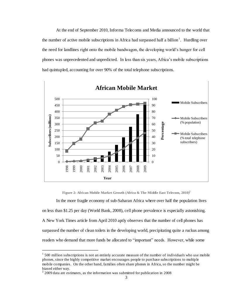
At the end of September 2010, Informa Telecoms and Media announced to the world that
the number of active mobile subscriptions in Africa had surpassed half a billion1. Hurdling over
the need for landlines right onto the mobile bandwagon, the developing world’s hunger for cell
phones was unprecedented and unpredicted. In less than six years, Africa’s mobile subscriptions
had quintupled, accounting for over 90% of the total telephone subscriptions.
Figure 2: African Mobile Market Growth (Africa & The Middle East Telecom, 2010)2
In the more fragile economy of sub-Saharan Africa where over half the population lives
on less than $1.25 per day (World Bank, 2008), cell phone prevalence is especially astonishing.
A New York Times article from April 2010 aptly observes that the number of cell phones has
surpassed the number of clean toilets in the developing world, precipitating quite a ruckus among
readers who demand that more funds be allocated to “important” needs. However, while some
1 500 million subscriptions is not an entirely accurate measure of the number of individuals who use mobile
phones, since the highly competitive market encourages people to purchase subscriptions to multip le
mobile companies. On the other hand, families often share phones in Africa, so the number might be
biased either way. 2 2009 data are estimates, as the informat ion was submitted for publication in 2008
0
10
20
30
40
50
60
70
80
90
100
0
50
100
150
200
250
300
350
400
450
500
1998
1999
2000
2001
2002
2003
2004
2005
2006
2007
2008
2009
Percen
tag
e
Su
bsc
rib
ers
(million
s)
Year
African Mobile Market
Mobile Subscribers
Mobile Subscribers
(% population)
Mobile Subscribers
(% total telephone
subscribers)
4
may complain that the modern focus misplaced on mobile phones above more imminent
necessities like clean water, adequate sanitation, and paved roads implies a gross caricature of
today’s obsession with technology, the reality is that mobile phones have revolutionized the
African economy. Though phone minutes and charging sometimes cost over half a family’s daily
wages, there are direct economic explanations for this widespread mobile popularity.
Perhaps the most avant-garde application of cell phones is mobile banking. For millions
of rural villagers who have never even seen a bank teller, cell phones are a ground-breaking
means of money transfer. M-Pesa (M stands for “mobile” and pesa is Swahili for “money”), first
introduced in Kenya and now spreading throughout Africa, is essentially a branchless banking
service through which customers can deposit and withdraw money via codes on mobile phones
from agents stationed in prominent marketplaces and other public areas. Previously, someone
sending money to friends or relatives had either the low-cost, high-risk option of sending money
physically with an intermediary on bus or by foot, or the high-cost, low-risk option of a post
office wire transfer. Enter M-Pesa. A husband working in Nairobi can now conveniently deposit
a thousand Kenyan shillings ($13) with an M-Pesa agent, the M-Pesa agent sends a text message
to the man’s family in a western province, and the wife can then redeem the text code at a local
M-Pesa agent for cash. “Secure, low-cost, convenient, and fast”, M-Pesa costs only forty percent
of the post office money transfer rate and twenty percent of the bus rate (Aker, 2010).
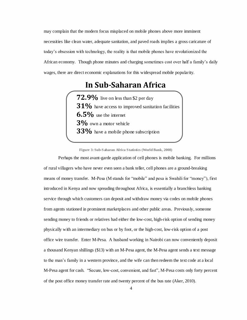
Figure 3: Sub-Saharan Africa Statistics (World Bank, 2008)
In Sub-Saharan Africa
72.9% live on less than $2 per day
31% have access to improved sanitation facilities
6.5% use the internet
3% own a motor vehicle
33% have a mobile phone subscription

5
Increased communication also leads to increased market transparency and fewer third
party inefficiencies. The age when farmers and fishermen paid outside dealers a small sum to
learn crop and fish prices at the market is becoming obsolete; local artisans can now text a market
salesman in the morning, learn the going prices
for the day, and then bring the most sought-after
products to the market in the evening. This
system not only decreases product waste and
increases profits, but also reduces variation
among salespeople and results in a better price
for households. Robert Jensen at Harvard
University estimates that in a small South Indian coastal city between 1997 and 2001, the time
period capturing the first introduction of phones to 60% penetration levels among fishermen and
market salesmen, violations of the Law of One Price decreased from 50-60% of market pairs to
essentially zero. As prices converge, arbitrage opportunities decrease and the net result is
positive for almost all parties. Jensen observes that “fishermen’s profits increased on average by
8 percent while the consumer price declined by 4 percent and consumer surplus in sardine
consumption increased by 6 percent.” Not only do people benefit from a monetary gain, but they
also save time as the consumer no longer has to shop between multiple vendors to get a fair price
and the fisherman no longer has to travel and find a physical third party to acquire market
information.
Without the aid of governments or subsidies or NGOs, the theoretical benefits of the
positive externality of mobile phones seem to materialize clearly in Africa and the rest of the
developed world. MIT studies claim that “adding an additional ten mobile phones per 100 people
boosts a typical developing country’s GDP growth by 0.6 percent” (EPROM, 2009). As
entrepreneurs innovate, regional-specific applications like M-Pesa emerge to serve a local need.
Figure 4: Fisherman in Chenai, India (©AP images/
America.gov, 2007)

6
As information becomes more readily available, market prices become more uniform and people
gain time and money on the whole. As communication is simplified, the burdens of finding
customers for a small business, organizing large numbers of volunteers for a service project, and
calling hospitals during an emergency are simultaneously alleviated.
1.2 The Challenge of Electricity
Pervasive and influential though mobile phones are, they may not be the “silver bullet” of
African development that some authors have proposed. There are significant obstacles for both
the provider and the consumer inherent to Africa’s long history of development and lack of
infrastructure.
Africa was once called the “Dark Continent” because it was such a mystery to European
explorers. Today, it carries the same name for a different reason – the absence of lighting in the
evening as shown by the NASA image in Figure 5. Consequently, the first setback for a cell
phone provider is the non-existent or
unreliable source of electricity in rural
areas, generating a significant start-up
cost for the project. As the nearest grid
is often hundreds of miles away,
providers often resort to off-grid diesel
or renewable sources to power their
stations. The high battery or generator
cost of the off-grid station is still less than the immense cost of connecting to the electric grid. As
a result, off-grid base stations far outnumber on-grid base stations in both South Asia and Sub-
Saharan Africa. The Global System for Mobile Communications Association (GSMA) predicts
Figure 5: Earth at Night (NASA, 2009)

7
that there will be 639,000 off-grid base stations in the developing world by 2012 (Taverner,
2010). While off-grid is not necessarily a negative aspect, renewable sources in particular
introduce added unpredictability. If a village has a week of cloudy or windless days, the tower
may well be out of service after the reserve battery life is drained.
The other setbacks for mobile operators in the developing world are more subtle with less
direct solutions. Imagine receiving a call to service a cell phone tower miles away on unpaved
roads or arriving at a station one morning to find the generator stolen and wires snipped. There
are obstacles both in the undeveloped environment itself and in impoverished populations that
always house a few desperate individuals willing to do anything for money. Customers often
bear this cost, resulting in higher per-minute charges in rural areas than urban areas. In Kenya,
Safaricom loses a vehicle a month on unpaved roads
and some mobile companies resort to armed guards to
protect their fuel, generators, and other equipment
from widespread theft (Ewing, 2007). Establishing a
new business in any area is difficult; with the
additional challenges of rampant theft and vandalism,
operators face unique maintenance hurdles.
In un-electrified areas, the primary obstacle
for the mobile consumer lies in the regular charging
of the cell battery. The NY Times featured an article
describing one Kenyan woman’s plight:
Every week, Ms. Ruto walked two miles to hire a motorcycle taxi for the three-hour ride to Mogotio, the nearest town with electricity. There, she dropped off her cell phone at a store that recharges phones for 30 cents. Yet the service was in such demand that she had
to leave it behind for three full days before returning (Rosenthal, 2010).
Figure 6: Charging Shop in Kiberia, Kenya
(GSMA)

8
Ms. Ruto is one of 500 million mobile users around the world without direct access to electricity,
according to GSMA and Wireless Intelligence research. These users typically pay per charge at a
local shop every week or every day, depending on their phone usage. In Kenya, it is estimated
that one-third of the mobile operating costs go to power instead of airtime (GSMA, 2010),
encouraging users to text rather than call whenever possible. More and more studies are being
conducted regarding off-grid mobile phone charging as companies grasp the magnitude of such a
market. When an individual gains access to a steady charging source, field studies suggest that
the mobile operator’s ARPU (average revenue per user) increases by at least ten percent because
the consumer feels comfortable making more calls. With 500 million customers, this
accumulates to a $2.3 billion market opportunity for network operators (GSMA, 2010).
1.3 Existing Solutions
Where there is an opportunity for profit, corporations and individuals will certainly rise to
the challenge. Digicel, Safaricom, and other mobile companies have already introduced solar
phones with miniature solar panels and batteries built into the back of the phone, allowing users
to leave their phone out during the day to charge. Safaricom and Ericsson have opened village
mobile charging stations in select areas monitored by a guard or other personnel, where people
can plug their phones into the charging dock for a small fee (GSMA, 2010). Since February
2009, GSMA, in partnership with mobile operators and manufacturers, has pioneered the
Universal Charging Solution initiative in hopes of standardizing all mobile chargers with an
energy-efficient micro-USB by 2012. Opening the possibility of a world without duplicate
chargers and with a 50% energy reduction in phone usage, this solution has garnered much
attention and many awards in the last two years.
9
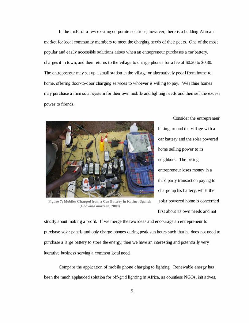
In the midst of a few existing corporate solutions, however, there is a budding African
market for local community members to meet the charging needs of their peers. One of the most
popular and easily accessible solutions arises when an entrepreneur purchases a car battery,
charges it in town, and then returns to the village to charge phones for a fee of $0.20 to $0.30.
The entrepreneur may set up a small station in the village or alternatively pedal from home to
home, offering door-to-door charging services to whoever is willing to pay. Wealthier homes
may purchase a mini solar system for their own mobile and lighting needs and then sell the excess
power to friends.
Consider the entrepreneur
biking around the village with a
car battery and the solar powered
home selling power to its
neighbors. The biking
entrepreneur loses money in a
third party transaction paying to
charge up his battery, while the
solar powered home is concerned
first about its own needs and not
strictly about making a profit. If we merge the two ideas and encourage an entrepreneur to
purchase solar panels and only charge phones during peak sun hours such that he does not need to
purchase a large battery to store the energy, then we have an interesting and potentially very
lucrative business serving a common local need.
Compare the application of mobile phone charging to lighting. Renewable energy has
been the much applauded solution for off-grid lighting in Africa, as countless NGOs, initiatives,
Figure 7: Mobiles Charged from a Car Battery in Katine, Uganda
(Godwin/Guardian, 2009)

10
and applications have been created for this specific purpose. However, by their intermittent
charging nature and existing technological structure, mobile phones, a much less-researched
topic, are even more conducive to renewable energy than lighting. Compared to lighting which
requires energy every evening after sundown, mobile phone charging is far more adaptable to the
individual. If the user knows he needs to make a long call the next day, he can prepare in
advance and fully charge his phone the day before. The time between charges is variable and
highly dependent on user behavior and decision-making. A prudent user, alerted by the
remaining battery life of his device, can plan his calls and charge accordingly to make the most
important calls at the best times. While renewable energy lighting requires an expensive battery
to store energy collected during the day, batteries are inherent to cell phones and entail no
additional investment. Thus, Africa, a continent latent with solar energy, coupled with mobile
phone charging and local entrepreneurship bridges a broad span of potential.
1.4 Overview
In this thesis, we examine the profitability of a small scale enterprise charging cell
phones from a solar module. Although there are many factors that affect profitability, we choose
to study the optimal pricing problem in depth, as this is the most salient numerical factor an
entrepreneur can control. Given prior intuition about the revenue generated using a discretized
set of prices, we seek to understand how the entrepreneur might logically develop pricing
strategies that utilize his prior belief, but also explore new prices. In Chapter 2, we gather market
information to specify cost and revenue assumptions in the particular context of Bababé,
Mauritania. This will be used as the basis of our prior belief on revenue in Chapter 3, where we
introduce the relevant notation and mathematical framework to use a correlated linear belief
structure in which the entrepreneur believes that revenue is a polynomial function of price.

11
In Chapter 4, we propose various policies to discover the optimal revenue. Representing
a diverse range of strategies, these policies fall into the main categories of myopic policies, value
function approximation policies, and look-ahead policies. Given these policies, we examine
worst case performance and average case performance with different prior beliefs in Chapter 5.
We investigate how the policies compare not only when the prior belief is close to the true
revenue distribution, but also when the entrepreneur has been overly optimistic or pessimistic in
his projections.
We provide a broad business framework in Chapter 6 to account for other aspects of the
enterprise besides optimal pricing. Supplemented by case studies with recent examples of a small
business and a large NGO’s successful use of solar power to charge phones and other applications,
the analysis is highly qualitative and discusses the cell phone charging market, customer, and
competition in more detail. The narrow view of Chapters 4 and 5 broadens to a wider scope in
Chapter 6 as we discuss the competitive advantage of a solar charging system and present ways to
improve the entrepreneur’s business model to minimize exogenous risk.
In the conclusion, we summarize the work to draw broad lessons and propose areas for
future research. In particular, we identify the key assumptions that are too restrictive and suggest
alternative approaches to the optimal pricing problem.

12
CHAPTER 2 Cost and Revenue Assumptions
Although business success is dependent on many factors, technical details aside, the most
important numerical factor an entrepreneur can control is price. If he believes that revenue is a
function of the price he charges, how does he choose the price that maximizes revenue? In reality,
the entrepreneur has a prior notion of the revenue he can garner at any given price and a strategy
to utilize his prior belief. He may, for example, take a game theoretical approach and just try to
undercut the price that his competitors at charging shops have set for a cell phone charge.
However, he is not sure that this is the true profit-maximizing price.
To clearly formulate the entrepreneur’s question, we first establish the macro
assumptions necessary to determine cost and revenue estimates. This entails current research on
both the solar industry on the cost side and the potential market of choice on the revenue side.
Note that although we have to make several assumptions about the true cost and revenue
distributions in a particular setting, this approach is easy to adapt to new situations when the truth
does not exactly mirror the suppositions proposed in this chapter.
13
2.1 Cost Assumptions
To estimate the entrepreneur’s initial capital expenditures at the onset of this start-up, we
must understand the fundamentals of solar technology and what traditional parts are necessary in
this context. Then we can study current market prices for various parts and obtain a basic cost
model for the solar module and other physical assets.
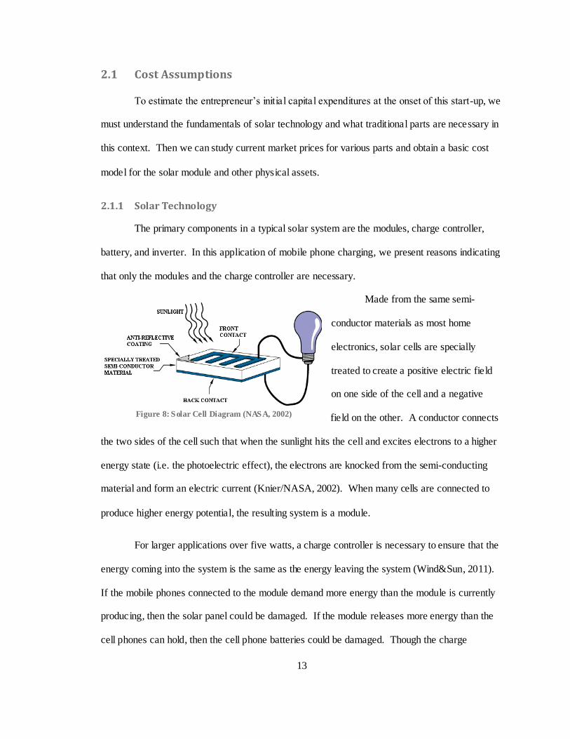
2.1.1 Solar Technology
The primary components in a typical solar system are the modules, charge controller,
battery, and inverter. In this application of mobile phone charging, we present reasons indicating
that only the modules and the charge controller are necessary.
Made from the same semi-
conductor materials as most home
electronics, solar cells are specially
treated to create a positive electric field
on one side of the cell and a negative
field on the other. A conductor connects
the two sides of the cell such that when the sunlight hits the cell and excites electrons to a higher
energy state (i.e. the photoelectric effect), the electrons are knocked from the semi-conducting
material and form an electric current (Knier/NASA, 2002). When many cells are connected to
produce higher energy potential, the resulting system is a module.
For larger applications over five watts, a charge controller is necessary to ensure that the
energy coming into the system is the same as the energy leaving the system (Wind&Sun, 2011).
If the mobile phones connected to the module demand more energy than the module is currently
producing, then the solar panel could be damaged. If the module releases more energy than the
cell phones can hold, then the cell phone batteries could be damaged. Though the charge
Figure 8: Solar Cell Diagram (NASA, 2002)

14
controller prevents both of these undesirable situations, Hankins in his guide Solar Electric
Systems for Africa reports that only half of the solar systems in Kenya took this precaution in
1995. Although people looking to make a quick profit may be frugal on up-front costs, their lack
of foresight ultimately has long term consequences as the life of the system is significantly
compromised. Improper care of photovoltaic systems has given solar a rather poor reputation in
Africa in past years, but with the correct maintenance and the more robust parts sold today, solar
is an exceedingly viable option as an off-grid power source.
A battery is necessary for most applications when the energy is not used as it is produced.
In lighting applications, for example, batteries store energy collected from the sun during the day
and release energy for lighting at night. In this entrepreneurial setting, a battery storage system is
redundant because we plan to only charge phones when the sun is shining. If there is a stretch of
cloudy days, it is assumed that customers will know that they cannot charge their phones until the
sun shines again, and will either find an alternative charging method or adjust their calling needs
appropriately.
Because electrons only travel one
direction in a module, solar applications usually
require an inverter to convert the direct current
(DC) energy collected from the sun into
alternating current (AC) energy required for most
home applications. Since cell phones are always
charged with direct current, the entrepreneur
has no need for an inverter unless he uses the
panel to charge other devices. In general, alternating current is used for most appliances because
it is easy to change voltage using a transformer. With alternating current, a power company can
Figure 9: How Solar Works (Young/QualityPoint
Technologies, 2010)

15
send electricity over long distances to homes using various voltages for safety and money-saving
reasons. Although low current allows electric companies to use smaller wires, high voltages are
also extremely dangerous. Thus, alternating current enables companies to exploit the tradeoff
between safety and speed in different areas.
For the entrepreneur in question, we only need to consider the solar module, charge
controller (for applications above five watts), and installation and set-up costs which include a
power strip to charge multiple phones at once.
2.1.2 Current Market Analysis
By examining current market prices for various solar components, we estimate the initial
cost for an entrepreneur setting up a solar micro-grid to charge phones. The most significant
upfront expense is the solar module, which consists of just over half the cost of the entire system,
as shown in the Frost & Sullivan breakdown in Figure 10. Because solar module prices are more
readily available than controller or
installation costs for the small applications
we evaluate for mobile charging3, we
estimate the controller and installation
costs as percentages of the module price.
To make the cost predictions as
general as possible, we approximate the
price of a solar module for a variety of
sizes. The power output is the most reliable indicator of price, since a compact, heavy solar panel
may have the same wattage as a large, light solar panel. Thus, by “size” we refer to wattage,
3 The average American home uses 11,040 kWh per year (US Energy In formation Admin istration, 2008),
or roughly 30 kWh per day. We are only considering s mall portable systems under 250W, the size o f a
small PV system used for camping or other s mall off-grid purposes.
Figure 10: Solar Cost Breakdown (Frost & Sullivan, 2009)

16
since weight and physical size are usually just indicators of the value of materials or the particular
design application, not necessarily indicators of price. The potential output of a solar module is
given by its power, measured in watts or watt-peak. Watt-peak is the output of a module under
standard conditions of 1000 watts per square meter of solar irradiance, but most literature uses the
term “watt” loosely to mean watt or watt-peak.
Although there is some variation in price per watt of various companies’ solar panels,
after combining the product information from nearly a hundred modules from various online solar
stores4, we observe a general economies of scale effect. The price graph is concave while the
price per watt graph is decreasing, indicating that the manufacturing cost per watt decreases as the
size of the system increases.
Figure 11: Solar Module Prices
We run a linear regression on the logarithm of price vs. the logarithm of watts to obtain
an exponential model for the cost of a solar module with x watts of the form:
The estimated coefficients a and b for the regression and their 95% confidence intervals are
shown in Figure 12. The confidence interval is computed by taking the standard error of the
residuals from the linear regression and transforming the coefficients into exponential form.
4 www.solar-for-energy.com, www.siliconsolar.com, www.wholesalesolar.com in January, 2011
$0
$200
$400
$600
$800
$1,000
-50 50 150 250
Pri
ce
Watts
Solar Module Price
$0.00
$5.00
$10.00
$15.00
0 50 100 150 200 250
Pri
ce p
er w
att
Watts
Solar Module Price Per Watt

17
Variability in the per-watt price is generally a result of differences in the quality of materials or in
the particular application for the solar panel. Panels created for frequent transportation or easy
portability are generally more expensive than typical modules.
Figure 12: Estimated Solar Module Price with 95% Confidence Interval
We use the exponential equations given in Figure 12 to estimate the total initial cost for
the entrepreneur. Assuming that the cost of a charge controller is roughly 20% of the cost of the
solar module itself and installation costs are slightly higher to include a power strip to charge
multiple phones simultaneously; we obtain a final estimate for the initial capital expenditures of
the entrepreneur:
Initial Capital Expenditures
Solar Modules (250W) $775.00
Charge Controller $150.00
Installation and Power Strip $200.00 Table 1: Initial Capital Expenditures
$0.00
$200.00
$400.00
$600.00
$800.00
$1,000.00
$1,200.00
0 50 100 150 200 250
Pri
ce
Watts
Estimated Solar Module Price
Original Data
Estimated
Upper Bound, with 95% Confidence
Lower Bound, with 95% Confidence
M(x) = 10.3391x0.8464
M(x) = 7.4654x0.7766
M(x) = 8.785x0.8115

18
Let us confirm that 250W is the maximum size necessary for this micro-enterprise.
Assuming a mobile phone takes 11.2Wh to charge5, a 250W module with five hours of sunshine
6
produces enough power to charge over 110 phones per day. In the revenue analysis to follow, we
see that this is the maximal size necessary for the entrepreneur who should only expect on
average 70 customers per day at low prices. In general, an entrepreneur can always add more
solar modules to his system, but he will probably only buy them in increments less than 250W
because of the high capital cost.
We must also estimate the weekly operating costs of the entrepreneur. Assume the
entrepreneur funds the entire project from a microfinance lender. Other options such as personal
savings or a loan from family or friends could also provide the initial capital needed, but we will
begin by assuming the higher interest rate and regular pay-back schedule of a microfinance loan,
leaving the discussion of other financing options to Chapter 6. Microfinance lending rates are
traditionally high because lenders cannot benefit from the economies of scale of large banks. The
microfinance process furthermore requires significant human capital costs to hire specialists to
train entrepreneurs and check up regularly on sma ll businesses. Accounting for high costs to
obtain small sums of money, the possibility of loan defaults, and high transaction costs, current
microfinance interest rates are close to 30% and sometimes as high as 40-50% (KIVA, 2011).
Solar is applauded for its low maintenance fees, so we set aside 0.1% of the initial cost of
the modules for maintenance each week. To garner business in the early weeks of the enterprise,
assume the entrepreneur hires an employee on commission for $0.01 per customer each day. He
then pays $0.01D(p) each week, where D(p) represents the weekly demand for phone charges at a
set price p. This advertising scheme is necessary for the first eight weeks, and then the
entrepreneur will be well-known enough to attract his own customers. And finally, the
5 7V and 0.8A over 2 hours charges a typical American phone (cellphoneshop.net, 2011)
6 Mauritania’s eastern neighbor Mali gets 5-7 peak watt hours per day (areed.org). Conservatively, we can
expect 5 peak watt hours per day for Mauritania.

19
entrepreneur must sustain his family. Assuming he takes $10 per week as pay and saves the rest
to invest in the business later, this yields the following estimate for weekly operating cost:
Operating Costs (weekly)
Loan Pay-back $31.20
Salary $10.00
Advertising (for the first 8 weeks) $0.01D(p)
Maintenance $0.78 Table 2: Weekly Operating Costs
2.2 Revenue Assumptions
Since revenue can be represented as revenue per customer times the number of customers,
an assumption about revenue implicitly includes an assumption about the number of customers
who will purchase charges at different prices, or in economic terms, the price elasticity of demand.
Mobile phone charging strikes an interesting balance between an inelastic and an elastic demand.
On one hand, no matter what the customer’s income or mobile phone usage patterns, he must find
a way to charge his phone. Whether in the city or in the local village, with a car battery or with a
generator, from a friend or from a stranger, the mobile phone battery must be charged. Perhaps
this is why the price of a charge is so high, forcing users to choose between charging their phones
and purchasing air-time. On the other hand, cell phone needs in Africa vary in degrees of urgency.
Some calls must be made right away, yet others can wait a few days or even be entirely forgone.
A prudent user knows how to juggle his needs to stretch his remaining battery life for a given
amount of time. Thus, while all phones must eventually be charged, customers have some control
over how often they want to charge their phones. Therefore, we expect a demand curve that is
neither perfectly inelastic nor perfectly elastic.
Revenue is a function of the price, but also a function of the population of the area and
the maximal market share. Though this analysis is fairly universal, it is helpful to contextualize

20
the entrepreneur and pick one specific area to study. We first provide an overview of a village in
Mauritania with high potential for solar energy and then discuss how to build a prior belief about
demand and revenue as a function of price in the following chapter. From the entrepreneur’s
perspective, we approximate the market demand for mobile phone charging, erring on the
conservative side for all numerical estimates.
2.2.1 Bababé, Mauritania
One of the poorest countries in Africa, Mauritania is a large, sparsely populated country
bordering the Atlantic Ocean, with population 3.3 million and annual GDP per capita $921 (USD).
A significant portion of Mauritania’s population live
on less than $1 a day, less than 50% have access to
an improved water source, and less than 25% have
access to improved sanitation. Poverty, as usual, is
most stark in rural communities (World Bank, 2011).
Although roughly three-quarters of the
country is desert, Mauritania is rich in natural
resources, as mining and iron ore account for nearly
half of the country’s exports. A historically nomadic
country, Mauritania’s main industries include
agriculture, livestock, and fishing. Severe droughts in the 1970’s greatly affected the country as a
result of heavy dependence on crops, accumulating much of the debt that still remains today.
Plagued historically by ethnic schisms and an entrenched practice of slavery, their recently-turned
republic has had a shaky start. President Taya was overthrown by a military coup in 2005 after
twenty years of authoritarian rule, shortly to be followed by another military coup in 2008.
Figure 13: Map of Mauritania (Geographic
Guide: Maps of Africa)
Bababé

21
The village of Bababé in the southwest corner of Mauritania has roughly 10,000 residents.
Households are fairly large in Mauritania since a typical family unit is built around the male head,
including his wives, children, parents, and unmarried sisters.
Regulated by the government through a Public-Private Partnership initiative, two diesel
generators currently provide electricity to 600 households and small businesses in Bababé
(Sohani, 2011). These generators currently run from 10am to 3am, but as the customer base
expands, it will be profitable for the generators to run all day and this will naturally threaten an
entrepreneur’s prospects at a successful solar charging industry.
2.2.2 Demand
We obtain a general approximation for cell phone charging demand in Bababé by
estimating the population of cell phone users without access to electricity. Note that in Africa the
percentage of people with access to electricity is much higher than the percentage that actually
have homes with solar panels or grid connections, since people often charge phones or watch TV
at the homes of friends and relatives. In 2009, there were 66.32 mobile subscriptions for every
100 people in Mauritania (International Telecommunications Union), a higher percentage than
those with improved water source access. Because Bababé is a smaller, more rural part of
Mauritania, we conservatively assume that cell phone coverage is closer to 35 subscriptions per
100 people. With the advent of electric generators, it is estimated that 50% of the population still
do not have access to electricity (Sohani), leaving a market of 1750 mobile users who need a
method to charge their phones. More realistically, the entrepreneur will probably only be able to
garner 10% of this market share even if he charges low prices, because each cell phone user
already has some existing way to charge their phone. Many have probably begun friendly
working relationships with bikers with car batteries and owners of local charging shops, so
convincing these people to switch to new-fangled solar technology may be more difficult than

22
merely charging a lower price. Averaging two cell phone charges a week and assuming the
entrepreneur only works five days per week, we expect the entrepreneur to have up to 70
customers per day for the lowest prices.
ESTIMATED SUPPLY QUANTITIES Low Est Med Est High Est
Solar hours per day (kWh/m2) 4 5 6
Watts produced per day 1000 1250 1500
Max phones can charge per day 89.29 111.61 133.93
ESTIMATED DEMAND QUANTITIES Low Est Med Est High Est
Population 9750 10000 10250
Cell phone users 2925 3500 4100
Cell phone users without electricity 1316.25 1750 2255
Customers per week if charged $.10 per charge 105.30 175 270.60
Customers per day if charged $.10 per charge 40.01 70 113.65
Table 3: Summary of Supply and Demand Assumptions

23
CHAPTER 3 Model
Central to the quantitative study of any real world problem is a clear and succinct
mathematical model that describes how we process relevant information. Given the assumptions
in the previous chapter, we introduce the Bayesian framework and notation necessary to make the
entrepreneur’s pricing decision. After proposing a revenue structure polynomial in price, we
utilize the previous chapter’s cost and revenue assumptions to obtain precise notions of both the
entrepreneur’s belief and the truth about the revenue that any price will generate. Using a
normal-normal model with linear beliefs, this entails specifying a mean and covariance structure
for the linear parameters. The last section of this chapter establishes the mathematical notation
needed to describe the process by which the entrepreneur makes weekly pricing decisions and
updates his belief about revenue with each new observation.
3.1 Linear Belief Structure
To determine an estimate for revenue as a function of price, we must have a notion of the
demand curve, the number of customers who will pay to charge their cell phones at a given price.
Intuitively, we know the demand curve is decreasing, because fewer people will charge their

24
phones at higher prices. From various newspaper articles and reports, we also know that the
going rate in Africa is $0.20 to $0.30 per charge (GSMA, 2010; Rosenthal/NY Times, 2010;
Edwards/Energy for Opportunity, 2011). However, beyond this basic knowledge, we can only
estimate. As we observe real demand values, Bayesian statistics later serves as a powerful tool to
update our prior belief and learn the true demand most efficiently.
Demand (D) and revenue (R) are both functions of price and are related by:
since revenue is simply the number of customers multiplied by the price paid per person. The
most simple and expressive form for the two functions is a polynomial function, linear in
coefficients. We choose a cubic demand model so that we can capture a logistic curve effect
when the demand is not as sensitive to price for extreme high or low prices. Revenue must
consequently be quartic because its degree is one greater than demand’s.
Although demand and revenue are non-linear with respect to price, they are both linear
with respect to the estimated parameters , and so the structure is correctly labeled a linear belief
model. With this structure, the entrepreneur only has to estimate the vector , and not the
individual values of R or D for the discrete set of prices.
In reality, the entrepreneur can only choose from a discrete set of prices, which can be
represented as an M X 1 vector with M alternatives, . Then we represent
the possible prices and corresponding revenues with vectors and R, respectively, and write the
above equation in shorthand:

25
(3.1)
where is an M X K matrix, and K is the number of linear terms in our model. Each row of is
the vector of terms corresponding to the coefficients.
(3.2)
Using a normal prior distribution and a normal sampling distribution, our belief about the
vector can be described by our belief about its mean vector and covariance matrix . We
use a normal-normal model to fully utilize our belief about covariance, the fact that we believe
the values and are related. If we are fairly certain, for example, that demand is
downward sloping and concave, then the linear and quadratic demand terms (corresponding to the
quadratic and cubic revenue terms) will be negatively correlated. For this reason among others,
we see the benefits of an additive linear belief model for demand. In addition to relating beliefs
about the general form of the demand curve, a linear belief structure is far more descriptive than a
regular correlated belief structure where the revenues for various prices are related. Imagine we
observe revenue much higher than what we believe is possible for a given price. The underlying
linear construction allows us to always update our belief about alternatives according to a natural
structure instead of arbitrarily making the belief about revenue for the observed price very high
and leaving the rest of the revenues low. Furthermore, the linear belief model reduces our
updating equations to only a K X K covariance matrix instead of an M X M matrix, and a K X 1
mean matrix instead of a M X 1 mean matrix. For a large number of alternatives, this
computational saving is immense.
The relationship between the mean and covariance of the parameters and the actual
alternatives p is given by simple linear algebra. Let us use the notation that after making n

26
observations of the true revenue, we believe the linear parameters are distributed normally
according to and the revenues are distributed normally according to
. is a K X 1 vector and is an M X 1 vector. It is already clear that =
by our linear assumption on revenue. The covariance between our beliefs at time n regarding two
prices and is given by:
(3.3)
where is the (i, k) entry of X.
Generalizing to matrix form, we can represent the M X M covariance matrix of the
alternatives by:
(3.4)
so that our belief about the alternatives normally distributed according to:
(3.5)

27
3.2 Specifying a Prior and a Truth Distribution
In the Bayesian model, we must specify two probability distributions for the vector.
The first is a distribution from which we generate the truth about revenue, and the second is a
distribution an entrepreneur might use as his initial belief before he begins to discover the truth.
To completely characterize the distribution in a normal-normal model, we must specify a mean
vector and a covariance matrix for both the prior and the truth. In reality, the truth is not
generated from a distribution; it simply exists and people try their best to discover it. However,
in this setting where we do not know the truth, but have an idea of what it might be, it is
necessary to establish a set of truths so we can observe the behavior of learning algorithms in
different states of the world and average them to see the broad behavior of the algorithm.
The learning process involves generating a true revenue curve and then using a learning
algorithm to discover that curve as fast as possible, starting with a prior belief about the revenue
curve. In the following sections, we first propose a truth distribution by doing a cubic regression
on point estimates of demand. Then, we generate a set of truths and determine the best, median,
and worst case scenarios for revenue. To provide a complete framework for the policy
optimization to follow, we finally propose various prior beliefs that an entrepreneur might have.
3.2.1 Truth Mean
Let us begin by assuming a true demand distribution of alternative means, since demand
for various prices is easier to visualize and estimate than revenue as a continuous function of
price. Although the linear belief model is more mathematically descriptive, it is also more
difficult to intuitively think of means and variances for values than it is to think of demand
approximations. After we assume demand point estimates, we use a cubic regression model to
obtain an estimate for the mean and covariance of the truth distribution, and .

28
Using the guidelines assumed earlier – that demand is a decreasing function of price and
less sensitive to price changes at extreme high or low prices, we propose the following numerical
low, medium, and high estimates for how demand should vary with price. Recall that the going
price is generally $0.20 to $0.30 per charge, so demand decreases significantly in this range, as
competition is stronger for these prices. Also, we are more certain about the behavior for extreme
prices, so the three estimates vary less for prices of $0.10 and $0.50 than for prices of $0.20 or
$0.30.
Price Med Est High Est Low Est
$0.10 350 360 340
$0.15 340 360 320
$0.20 300 340 240
$0.25 225 310 140
$0.30 150 250 70
$0.35 100 175 30
$0.40 60 100 15
$0.45 30 50 5
$0.50 10 20 0
Table 4: Estimates for True Demand at
Various Prices
Figure 14: Point Estimates for True Demand
Means
Given these point estimates, we calculate the linear parameters corresponding to our
belief by running cubic regressions on these three curves. The cubic regressions yield the
following results for the three demand estimates:
Estimated
Med 11144.78 -9482.68 1386.75 301.27
High 11750.84 -11984.85 2703.20 192.22
Low 9158.25 -5876.62 -171.92 422.66 Table 5: Theta Estimates for True Demand
0
50
100
150
200
250
300
350
400
0 0.2 0.4 0.6
Cu
sto
mers
per w
eek
Price
Point Estimates for True
Demand
Med
High
Low

29
3.2.2 Truth Covariance
Since estimates for the standard deviation of the values given by the regressions are
extremely high, we use half of the absolute value of an average of the difference of the estimated
’s as proxies for standard deviation. That is,
This can also be viewed as though we want our high and low estimates of the demand to be two
standard deviations above and two standard deviations below our best estimates when we
generate truths. Since the estimates are not exactly centered on the medium estimate, we take an
average of the two differences. This short exercise also makes it clear that for the desired shape
of the demand curve, and are negatively correlated with and . When one group
increases, the other decreases.
With estimates for the standard deviations of each term, we create a covariance matrix
to generate truths. Because a slight change in proportions of the terms yields drastically
different results, we set a very high correlation co-efficient between and , for all
. Then, each element of the covariance matrix for truths is:
Using the mean vector and covariance matrix as described, we produce 99 truths from the
distribution, shown in Figure 15(a).

30
Figure 15: 99 Generated Truths
3.2.3 Prior Mean
Let us now determine reasonable prior beliefs that an entrepreneur might have. Of course,
the entrepreneur could use the mean and covariance matrix we just used to generate the truth, but
he might also have less sophisticated beliefs. We use four prior distributions in the analysis of
Chapter 5:
1. Truth: a prior which is the same as the mean used to generate the truth.
2. Linear: a prior with a linear belief about demand and hence a quadratic belief about
revenue, in which demand decreases linearly from 70 customers per day at $0.10 to 0
customers per day at $0.50.
3. Optimistic: a prior in which the entrepreneur generates $80 in revenue per week,
regardless of the price he sets.
4. Pessimistic: a prior in which the entrepreneur generates $10 in revenue per week,
regardless of the price he sets.
0.1 0.15 0.2 0.25 0.3 0.35 0.4 0.45 0.50
20
40
60
80
100
120
99 truths for revenue
Price to charge one cell phone
Weekly
Revenue (
$)
0.1 0.15 0.2 0.25 0.3 0.35 0.4 0.45 0.50
50
100
150
200
250
300
350
400
450
50099 truths for demand
Price to charge one cell phone
Weekly
Dem
and (
custo
mers
)
Figure 15(a): 99 Truths for Revenue Figure 15(a): 99 Truths for Demand
31
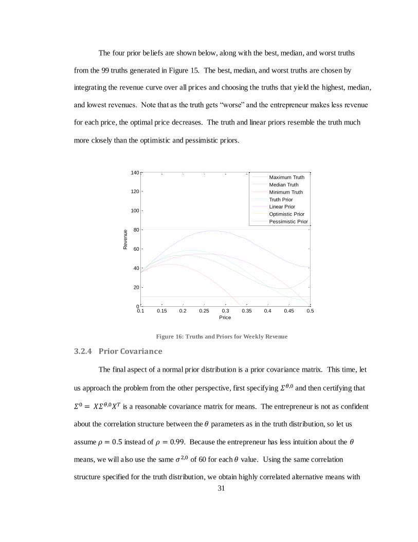
The four prior beliefs are shown below, along with the best, median, and worst truths
from the 99 truths generated in Figure 15. The best, median, and worst truths are chosen by
integrating the revenue curve over all prices and choosing the truths that yield the highest, median,
and lowest revenues. Note that as the truth gets “worse” and the entrepreneur makes less revenue
for each price, the optimal price decreases. The truth and linear priors resemble the truth much
more closely than the optimistic and pessimistic priors.
Figure 16: Truths and Priors for Weekly Revenue
3.2.4 Prior Covariance
The final aspect of a normal prior distribution is a prior covariance matrix. This time, let
us approach the problem from the other perspective, first specifying and then certifying that
is a reasonable covariance matrix for means. The entrepreneur is not as confident
about the correlation structure between the parameters as in the truth distribution, so let us
assume instead of . Because the entrepreneur has less intuition about the
means, we will also use the same of 60 for each value. Using the same correlation
structure specified for the truth distribution, we obtain highly correlated alternative means with
0.1 0.15 0.2 0.25 0.3 0.35 0.4 0.45 0.50
20
40
60
80
100
120
140
Price
Revenue
Maximum Truth
Median Truth
Minimum Truth
Truth Prior
Linear Prior
Optimistic Prior
Pessimistic Prior

32
standard deviations of near 60-70. This is reasonable for our entrepreneur, who probably has
little idea what the true revenue for any price is. Now, with a specific set of truth and prior
distributions, we explore which policies are most effective at learning the truth in Chapter 5.
3.3 Mathematical Model
Given a prior belief about the coefficients of a linear model, we describe the revenue
learning process. The entrepreneur makes a pricing decision based on his prior belief, observes a
noisy instance of the true revenue at that price, and updates his linear belief structure using
Bayesian statistics. In this correlated linear belief model, one observation of price changes the
entrepreneur’s belief about all the coefficients in his model. We assume that the entrepreneur
can change price once per week, so time is indexed by n measured in weeks. Using Powell’s
notation (2010) to define the entrepreneur’s pricing problem, we express the entrepreneur’s
process of learning consumer demands by his state variable, exogenous information, decision,
transition function, and contribution.
3.3.1 State Variable
The state variable is defined as “the minimally dimensioned function of history that is
necessary and sufficient to compute the decision function, the transition function, and the
contribution function” (Powell, 2010). Thus, the state variable captures all the knowledge
necessary to the decision-making process. We use the general notation that superscript n
indicates information known at week n, after making n measurements. Any information with
superscript is random at week n, but known at week . The state of the enterprise after n
price measurements includes the entrepreneur’s belief about the mean and covariance of the
coefficients that guide the general revenue equation (3.1). It is written as follows:

33
By convention, the state variable only includes dynamic information that is updated over time.
Other static information necessary for computation are considered parameters, such as the matrix
X and the measurement noise .
3.3.2 Exogenous Information
We know that the true revenue is a function of price, but even with an unchanging truth
we only obtain imperfect observations of revenue because of measurement noise. In this setting,
exogenous information is the random revenue generated from setting a certain price x.
where =
and the measurement noise is normally distributed according to .
3.4.3 Decision
The entrepreneur’s primary decision is which price to set for a mobile phone charge on
week n. In Chapter 4, we propose different policies to make such a pricing decision, but for now,
we write in general notation:
where is the price chosen on week n and is a decision made by using policy from a
given state .
3.3.4 Transition Function
As mentioned before, the power of the Bayesian model lies in the fact that the
entrepreneur updates his belief each time period based on the price he chose and the
corresponding revenue observation. Using the state notation introduced above, the entrepreneur
updates his state based on the model M according to:

34
The recursive updating equations are described more thoroughly in both Powell and Ryzhov
(2010) and Negoescu et al. (2009), but here we present the results without proof. and are
just intermediate calculations used to simplify the notation.
(3.6)
(3.7)
(3.8)
(3.9)
where is a column vector containing the row entries of X corresponding to the price chosen
on week n:
3.3.5 Contribution Function
The entrepreneur’s goal is to maximize his total profit, the difference between revenue
and cost. By the assumptions given in Chapter 2, we give the weekly contribution of making a
particular decision in state as:
(3.10)
where is the cost for the entrepreneur as a function of revenue, since he pays
advertising costs as a portion of revenue in the early weeks of the business. This current profit
for a single period specifies how we determine the efficacy of a policy. By summing the
contribution over each period to obtain cumulative profit, we know which policies are most
effective in profit generation.
CHAPTER 4 Policy Optimization Overview
Posed with the problem of choosing an optimal price, the entrepreneur has several
decision-making options. After checking market prices for mobile charges in comparable
businesses and estimating their weekly demand, he formulates a prior belief in a manner similar
to our analysis in the previous chapter. Recall that a prior distribution includes a belief about the
mean and the covariance of various prices, so the entrepreneur must quantify both his intuition
regarding the revenue that various prices will yield as well as the uncertainty he has for each
estimate. Given this prior belief, the entrepreneur is faced with the classic “exploration-
exploitation” question of decision-making. He must balance exploiting his hunch about the
optimal price and exploring new prices that he is uncertain about, in fear that his original belief
was wrong. If the entrepreneur’s intuition is correct, then an exploitation policy is optimal. Yet
in the more likely event that the entrepreneur’s belief is not entirely correct, the best general
policies allow for a balanced mixture of exploration and exploitation and thus permit the
entrepreneur to learn the best price over time.
In this chapter, we examine several decision-making policies and introduce an additional
pricing restriction to mirror the actual situation more closely. The pricing problem is part of a
widely studied class of ranking and selection problems in which the decision maker must choose
one of many alternatives to measure in each time period, given a measurement budget. In this
36
online context with correlated beliefs, the revenue from each period accumulates over time and
the entrepreneur believes that the revenues from various prices are not independent.
For a summary of correlated belief research in ranking and selection, see Frazier et al.
(2009) and for a description of online policies, see Ryzhov et al. (2010). The most common
solution to the online “multi-armed bandit problem” in which early decisions affect the final
objective function is the Gittins index policy (Gittins (1974)), chosen to be optimal for an infinite
measurement budget with discounted rewards. To avoid the difficult computation of Gittins
indices, the knowledge gradient policy maximizes the value of making an additional
measurement (see Frazier et al. (2009) for initial derivation and Ryzhov et. al (2010) for
extension to the online case).
However, in all the policies mentioned thus far, the problem size is still linear in the
number of alternatives. Because it is ideal to analyze the pricing problem with a continuous
alternative set, we choose to analyze a revenue structure that is linear in its parameters instead,
thus simplifying the problem from an infinite alternative set to a small number of parameters. It
is possible, of course, to use existing policies to choose an alternative and then update the
parameters according to Bayesian updating equations, but few policies exist specifically for this
linear belief framework. In the context of drug discovery, an adaptation of Frazier’s knowledge
gradient policy for an additive linear model is proposed by Negoescu et al. (2009), and we
compare this policy to others in Chapter 5.
To adapt to the entrepreneur’s pricing problem to the ranking and selection framework,
we discretize the alternative set so that the only available prices during any time period are in
increments of $0.05 between $0.10 and $0.50 per cell phone charge. Many simple algorithms for
the ranking and selection problem have been suggested (see Powell and Ryzhov (2010) for more
details), each with favorable qualities and unfavorable shortcomings. The first pure exploitation
policy describes what is most likely to happen in reality as an entrepreneur chooses whatever

37
price he believes at that time will generate optimal revenue. The entrepreneur only takes into
account his profit for the current period in this classic myopic policy. The next three policies,
Boltzmann exploration, interval estimation, and upper confidence bounding are in a class of value
approximation policies that describe metrics for assigning values to alternatives. They seek a
finer balance between exploration and exploitation based on how much better we believe an
alternative is than its peers, how uncertain we are about an alternative, and how many times we
have already measured an alternative. In a different class of look-ahead policies, knowledge
gradient and decision tree resemble a more sophisticated entrepreneur who projects his current
beliefs into the future and makes decisions that maximize reward over a period of time.
4.1 Pure Exploitation
A very confident entrepreneur would use a pure exploitation policy that simply chooses
whatever price he believes is best each week. After observing a price, he updates his belief as
given in (3.6) - (3.9) and then chooses again what he believes is best. We use the notation that
is the price chosen on week n given some policy on the current belief state. That is,
. Recall that the belief state includes an estimate about the mean and
covariance matrix of the revenues for each price alternative x.
The pure exploitation policy can then be written as:
(4.1)
as the entrepreneur chooses the price he believes yields the highest mean revenue. Although this
policy has great potential if the entrepreneur’s prior belief is very accurate, it also has little
chance of discovering the true optimal price in any other case.

38
4.2 Boltzmann Exploration
This “soft max” policy picks a price to measure probabilistically, picking prices that the
entrepreneur believes yield more revenue with high probability. It samples each alternative x
with probability:
(4.2)
where is a tunable parameter such that for small , the policy samples each alternative with
equal probability (pure exploration), but for large , the policy samples the alternative with
the highest mean with probability one (pure exploitation). We simulate the policy over many
truths, and pick the that maximizes our expected profit. Then, the Boltzmann policy specifies
that we choose an alternative probabilistically according to:
4.3 Interval Estimation (IE)
The interval estimation method is based on the concept of a confidence interval. The
entrepreneur believes that of the time, the sample revenue will fall within the
interval
where is the estimated standard deviation of
, found by
taking the corresponding diagonal term of the covariance matrix . As usual,
), leaving in the upper tail of the standard normal distribution.
If the entrepreneur was to create confidence intervals with confidence level for the
revenue expected for each price, and pick the price with the highest upper bound of the
confidence interval, he would choose according to the following equation:
(4.3)
In this case, the confidence level has no real meaning and is simply treated as a tunable
parameter like in the Boltzmann exploration case. For small , interval estimation acts
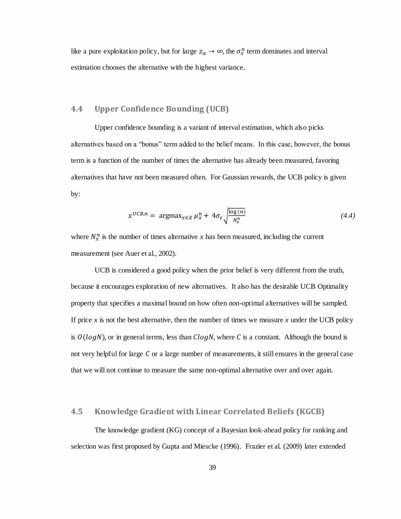
39
like a pure exploitation policy, but for large , the term dominates and interval
estimation chooses the alternative with the highest variance.
4.4 Upper Confidence Bounding (UCB)
Upper confidence bounding is a variant of interval estimation, which also picks
alternatives based on a “bonus” term added to the belief means. In this case, however, the bonus
term is a function of the number of times the alternative has already been measured, favoring
alternatives that have not been measured often. For Gaussian rewards, the UCB policy is given
by:
(4.4)
where is the number of times alternative x has been measured, including the current
measurement (see Auer et al., 2002).
UCB is considered a good policy when the prior belief is very different from the truth,
because it encourages exploration of new alternatives. It also has the desirable UCB Optimality
property that specifies a maximal bound on how often non-optimal alternatives will be sampled.
If price x is not the best alternative, then the number of times we measure x under the UCB policy
is , or in general terms, less than , where is a constant. Although the bound is
not very helpful for large or a large number of measurements, it still ensures in the general case
that we will not continue to measure the same non-optimal alternative over and over again.
4.5 Knowledge Gradient with Linear Correlated Beliefs (KGCB)
The knowledge gradient (KG) concept of a Bayesian look-ahead policy for ranking and
selection was first proposed by Gupta and Miescke (1996). Frazier et al. (2009) later extended
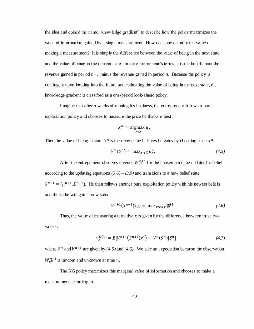
40
the idea and coined the name “knowledge gradient” to describe how the policy maximizes the
value of information gained by a single measurement. How does one quantify the value of
making a measurement? It is simply the difference between the value of being in the next state
and the value of being in the current state. In our entrepreneur’s terms, it is the belief about the
revenue gained in period n+1 minus the revenue gained in period n. Because the policy is
contingent upon looking into the future and estimating the value of being in the next state, the
knowledge gradient is classified as a one-period look-ahead policy.
Imagine that after n weeks of running his business, the entrepreneur follows a pure
exploitation policy and chooses to measure the price he thinks is best:
Then the value of being in state is the revenue he believes he gains by choosing price :
(4.5)
After the entrepreneur observes revenue for the chosen price, he updates his belief
according to the updating equations (3.6) – (3.9) and transitions to a new belief state
. He then follows another pure exploitation policy with his newest beliefs
and thinks he will gain a new value:
(4.6)
Thus, the value of measuring alternative x is given by the difference between these two
values:
(4.7)
where and are given by (4.5) and (4.6). We take an expectation because the observation
is random and unknown at time n.
The KG policy maximizes this marginal value of information and chooses to make a
measurement according to:

41
(4.8)
The derivation of the KG policy for correlated linear beliefs (KGCB) is shown by Negoescu et al.
(2009), but we present the results here without proof. The policy is given by:
(4.9)
where
is the xth row of the original X matrix given in (3.2) and Z is a standard normal random
variable. is a vector giving the change in the variance of the entrepreneur’s belief about
the set of alternatives after measuring option x and is a function we maximize over.
Negoescu et al. (2009) also suggest an algorithm to calculate without taking an explicit
expectation, but we omit the details here.
4.6 Decision Tree (DT)
Decision trees are commonly used in the operations research and machine learning
communities to depict the flow of decisions and random information in a way that is easy to
visualize. A clear and concise overview of the current popular literature on decision trees can be
found in Utgoff (2010) and we summarize his findings here.
In a world with increasingly complex decisions, decision trees arose out of a need to
model and automate the way a rational person makes decisions. They are often used in the
medical field to trace the factors a doctor must consider to make a diagnosis or prescription.
Although decision trees can also be used to model categorical data (i.e. a classification tree), we
are only interested in modeling quantitative data (i.e. a regression tree) in this application.
Decision trees are usually computed using top-down recursion (see Friedman, 1977 for a
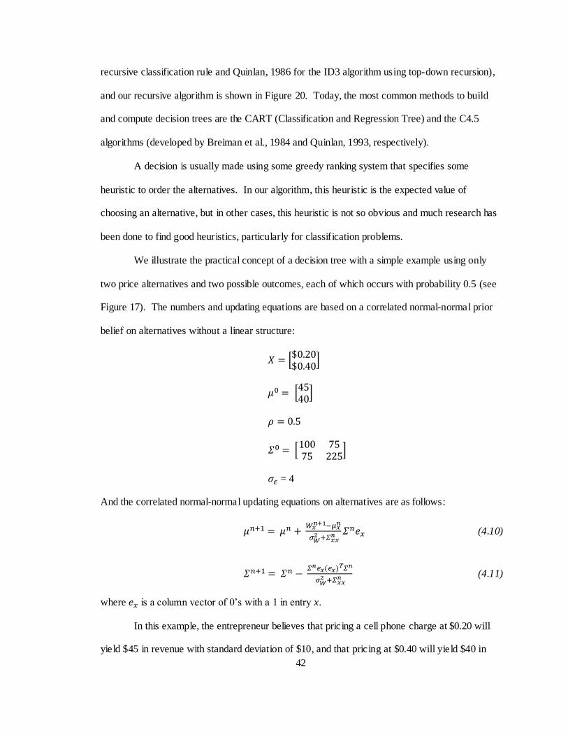
42
recursive classification rule and Quinlan, 1986 for the ID3 algorithm using top-down recursion),
and our recursive algorithm is shown in Figure 20. Today, the most common methods to build
and compute decision trees are the CART (Classification and Regression Tree) and the C4.5
algorithms (developed by Breiman et al., 1984 and Quinlan, 1993, respectively).
A decision is usually made using some greedy ranking system that specifies some
heuristic to order the alternatives. In our algorithm, this heuristic is the expected value of
choosing an alternative, but in other cases, this heuristic is not so obvious and much research has
been done to find good heuristics, particularly for classification problems.
We illustrate the practical concept of a decision tree with a simple example using only
two price alternatives and two possible outcomes, each of which occurs with probability 0.5 (see
Figure 17). The numbers and updating equations are based on a correlated normal-normal prior
belief on alternatives without a linear structure:
= 4
And the correlated normal-normal updating equations on alternatives are as follows:
(4.10)
(4.11)
where is a column vector of 0’s with a 1 in entry x.
In this example, the entrepreneur believes that pricing a cell phone charge at $0.20 will
yield $45 in revenue with standard deviation of $10, and that pricing at $0.40 will yield $40 in

43
revenue with standard deviation $15. He thus has to choose between the price which leads to
higher revenue and the price which leads to a more uncertain revenue, according to his current
belief. In the following figure, the square nodes are decision nodes where the entrepreneur has to
choose between the two prices and the circular nodes are outcome nodes where the entrepreneur
observes a random outcome with certain probability.
Figure 17: Decision Tree (Initial)7
For sake of clarity, we simplify the problem considerably in this diagram so that at Level
(1a) of the tree, the entrepreneur only has two pricing options: $0.20 and $0.40. If the
7 All probabilities in Level (2b) of the tree are also 0.5, but are omitted for visual simplicity.
Level (1a) Level (1b) Level (2a) Level (2b) Level (3)

44
entrepreneur picks a price of $0.20 this week, then according to his prior belief, he thinks he can
make either $35 or $55 in revenue with equal probability (shown in the Level (1b) outcome
nodes). This is also a simplification of the normal-normal model, assuming that in a
discretization of the normal distribution , we observe an outcome:
(4.12)
Pretending that he actually observes these values, the entrepreneur then updates his prior
belief to predict new outcomes in Level (2b), enumerating possible revenues given his choice in
Level (1a). Note the effect of the updating equations. The entrepreneur’s belief about revenue
for a price of $0.20 or $0.40 in Level (2b) is higher if he observes high revenue in Level (1b) than
if he observes low revenue. This is a result of updating within the tree, as the entrepreneur tries
to mimic his exact decision-making process over time.
To make a single decision, the entrepreneur projects his beliefs into the future, calculates
the profit gained from any possible pathway (Level (3)), and iterates backward from the end of
the tree to find the optimal decision. Each outcome node is replaced by the expected value of
choosing a certain price, and each decision node chooses the price that maximizes the expected
outcome. See Figure 18 for the sample decision tree after iterating one step backwards in the tree
where the highlighted lines represent the price chosen from each decision node.

45
Figure 18: Sample Decision Tree (One Iteration Back)
The outcome nodes in Level (2b) now just give the expected value of making a decision
in Level (2a). A rational entrepreneur would choose the price in Level (2a) that maximizes his
expected revenue, and thus, as we iterate backwards to Level (1) of the tree, we replace each
decision node with the values from the highlighted decision. Then we repeat the same exercise
and take the expected value of these numbers to obtain Figure 19.
Level (1a) Level (1b) Level (2a) Level (2b)

46
Figure 19: Sample Decision Tree (Two Iterations Back)
From this simplified decision tree analysis, we see that the entrepreneur maximizes his expected
reward by choosing a price of $0.20 in the current time period.
The decision tree is a discretized, multiple look-ahead period version of the knowledge
gradient policy with added ability to change sampling distributions or implement other
restrictions easily, but without the mathematical elegance of the KG formula. Notice that even
though we “make decisions” for multiple intermediate steps in the tree, the only real decision we
implement is the first node. Then we observe a revenue sample, update our beliefs, and draw a
new tree for the current time period.
4.7 Restricted Pricing
One unique aspect to this revenue problem in the context of other ranking and selection
literature is that of pricing psychology. If an entrepreneur bounces between charging $0.10 and
$0.50 for a mobile charge each week, customers will soon become exasperated with the volatile
pricing scheme and go to the nearest competitor who can actually decide on a decent price. Or
Level (1a) Level (1b)

47
perhaps customers will just wait for the next $0.10 charge since they know the $0.50 price will
not remain for long. In all respects, it is best for the entrepreneur to keep price fluctuation
between weeks as low as possible. Thus far, in the traditional ranking and selection problem and
policies, we assume that the same alternative set is available each week. In any time step, the
entrepreneur can potentially choose any of the M prices. However, to refine this model further,
we now add a new dimension – a restricted pricing set. An entrepreneur can only price charges
within $0.10 of last week’s price.
This restriction can be implemented in all the policies in a simple manner. Let the policy
choose the alternative it would normally choose. Then modify this choice as follows:
(4.13)
If is not within $0.10 of the previous week’s choice, then choose the closest price to the
originally chosen alternative in the restricted set. If is within $0.10 of the previous week’s
choice, then let .
Without significant re-derivation, all of the policies except the decision tree lack the
ability to anticipate how this pricing restriction will affect future decisions. However, in the
decision tree, it is very simple to foresee this restriction by just expanding the tree on the
alternatives within $0.10 of the past price. If the last alternative chosen was an extreme price,
then we expand on the five alternatives nearest to the price endpoint. This has the additional
advantage of “pruning” the decision tree and greatly improving its computation time. Because a
decision tree with K alternatives, L discretized observations, and M look-aheads has paths
to evaluate, many methods have been proposed to prune the decision tree to reduce K. See

48
Mingers (1989) for an empirical comparison of five pruning methods based on training sets and
valuation methods to determine the importance of a given node.
Because the decision tree grows polynomially with the number of alternatives or
discretizations, and exponentially with the number of look-aheads, it is important to limit each of
these factors to small, yet still descriptive, numbers. In our full decision tree implementation, we
allow the entrepreneur to pick any of the alternatives each time period, but when simulating the
decision tree into the future, we only expand on restricted alternatives. This is only for the sake
of computational savings; it does not accurately reflect how the entrepreneur actually thinks about
his decisions. In the restricted implementation of the decision tree, each decision node has five
alternatives. If pricing psychology is taken into consideration, this accurately mirrors an
entrepreneur’s actual decision-making thought process, as he knows that the price he chooses
today will certainly affect the price he can choose next week.
In both the full and restricted trees, we discretize each outcome node into five possible
outcomes by taking equally spaced portions of the normal distribution, each outcome with
probability 0.2 of occurrence. And finally, since the restricted tree with M look-ahead periods has
paths and the regular decision tree has paths, we limit the number of look-
aheads to 3.
To summarize these points more lucidly, we give the restricted decision tree
implementation below, where the Decision Tree algorithm calls the recursive Build Tree
algorithm each time it makes a decision. To edit the policy for the full decision tree described,
we just initialize the price set in the Decision Tree algorithm to the full set of alternatives, instead
of the restricted set.
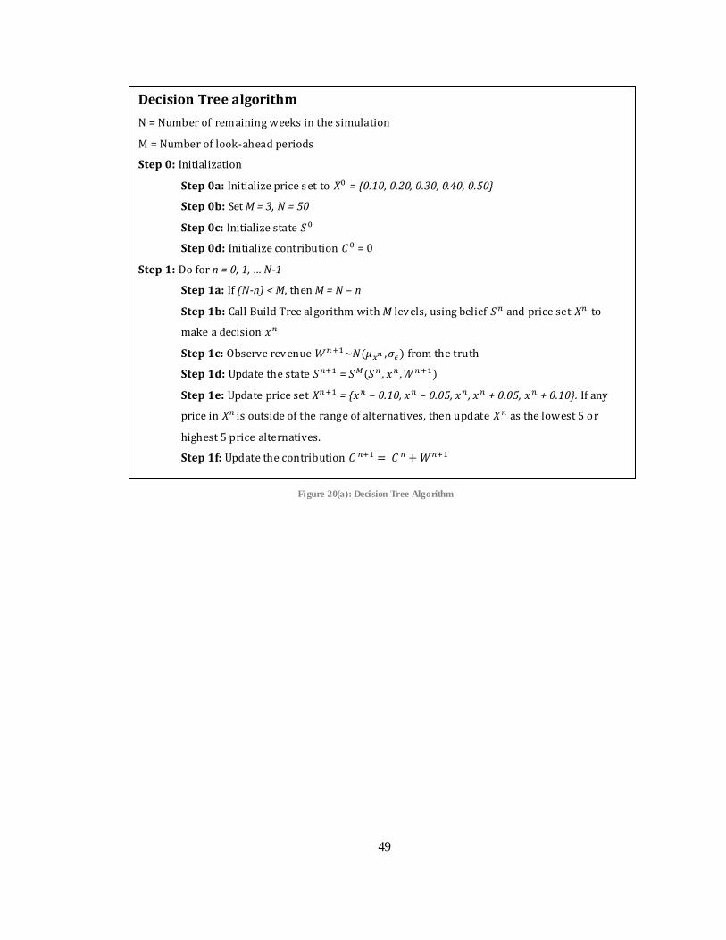
49
Decision Tree algorithm
N = Number of remaining weeks in the simulation
M = Number of look-ahead periods
Step 0: Initialization
Step 0a: Initialize price set to = {0.10, 0.20, 0.30, 0.40, 0.50}
Step 0b: Set M = 3, N = 50
Step 0c: Initialize state
Step 0d: Initialize contribution = 0
Step 1: Do for n = 0, 1, … N-1
Step 1a: If (N-n) < M, then M = N – n
Step 1b: Call Build Tree al gorithm with M levels, using belief and price set to
make a decision
Step 1c: Observe revenue from the truth
Step 1d: Update the state =
Step 1e: Update price set = { – 0.10, – 0.05, , + 0.05, + 0.10}. If any
price in is outside of the range of alternatives, then update as the lowest 5 or
highest 5 price alternatives.
Step 1f: Update the contribution
Figure 20(a): Decision Tree Algorithm
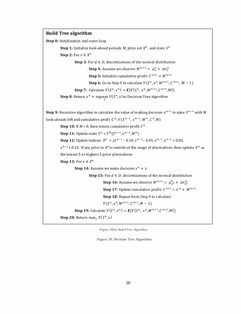
50
Build Tree algorithm
Step 0: Initialization and outer loop
Step 1: Initialize look-ahead periods M, price set , and state
Step 2: For
Step 3: For , discretizations of the normal distribution
Step 4: Assume we observe
Step 5: Initialize cumulative profit:
Step 6: Go to Step 9 to calculate
Step 7: Calculate
Step 8: Return
to Decision Tree algorithm
Step 9: Recursive algorithm to calculate the value of making decision in state with M
look-aheads left and cumulative profi t :
Step 10: If M = 0, then return cumulative profit
Step 11: Update state =
Step 12: Update indices: { – 0.10, – 0.05, , + 0.05,
+ 0.10. If any price in is outside of the range of al ternatives, then update as
the lowest 5 or highest 5 price al ternatives.
Step 13: For
Step 14: Assume we make decision
Step 15: For , discretizations of the normal distribution
Step 16: Assume we observe
Step 17: Update cumulative profi t:
Step 18: Repeat from Step 9 to calculate
Step 19: Calculate
Step 20: Return
Figure 20: Decision Tree Algorithm
Figure 20(b): Build Tree Algorithm
51
CHAPTER 5 Policy Optimization Analysis
If an entrepreneur was actually to use the learning algorithms in the previous chapter to
find the optimal price, his potential profit and risk would vary according to the selected policy
and the accuracy of his prior belief. In this chapter, we compare policies in various contexts to
determine which perform the best in the worst case and on average.
Worst case analysis is perhaps the most important as it signals to investors that the
entrepreneur has carefully considered potential risks and is not running carelessly with an idea
that sounds much better on paper than it is in practice. By showing the results of the algorithms
when revenue prospects are lowest, we obtain a general idea of how poorly this enterprise might
fare and how an extremely cautious entrepreneur might proceed to choose prices week by week.
Following worst case analysis, we compare restricted and unrestricted policies in the
general case averaged over many truths generated from the distribution specified in Chapter 3.
Although four possible revenue priors are described in Chapter 3, we only include analysis for the
prior that is the same as the truth distribution and the prior that is overly optimistic as examples of
“good” and “bad” priors, respectively. The same results for linear and overly pessimistic priors,
additional examples of “good” and “bad” priors, are given in the appendix. Through this average
case analysis, we seek to understand a number of practical questions such as how profit depends

52
on the truth distribution’s maximal revenue and how the value function approximation and look-
ahead policies compare to pure exploitation, the entrepreneur’s default strategy. With these
predictions, we furthermore obtain basic profitability estimates over the first weeks of the
entrepreneur’s business. As in the cost and revenue estimates of Chapter 2, we err on the most
conservative side and consequently only give simulated results for the first year of the business,
when costs are the highest as the entrepreneur pays back his micro-finance loan.
5.1 Worst Case Analysis
For the worst case truth, it is almost impossible for the entrepreneur to make a profit
above his regular salary under the given cost assumptions. Costs, including loan payments, are
between $40 and $45 per week and maximum potential revenue is only $43 if we price $0.15 per
cell charge. The true mean revenue in the worst case for the various prices is shown below, along
with the measurement variance of each price and the linear prior belief about each alternative.
(price)
$0.10 $35.24 $4 $35.00
$.15 $43.05 $4 $45.93
$.20 $42.14 $4 $52.50
$.25 $32.47 $4 $54.68
$.30 $15.59 $4 $52.50
$.35 $0 $4 $45.94
$.40 $0 $4 $35.00
$.45 $0 $4 $19.69
$.50 $0 $4 $0
Table 6: Worst Case Truth and Linear Belief Means
Unless the entrepreneur finds the optimal price within the first few weeks, he cannot sustain his
enterprise. If the entrepreneur starts with $75 cash initially and a belief that demand is linear, his
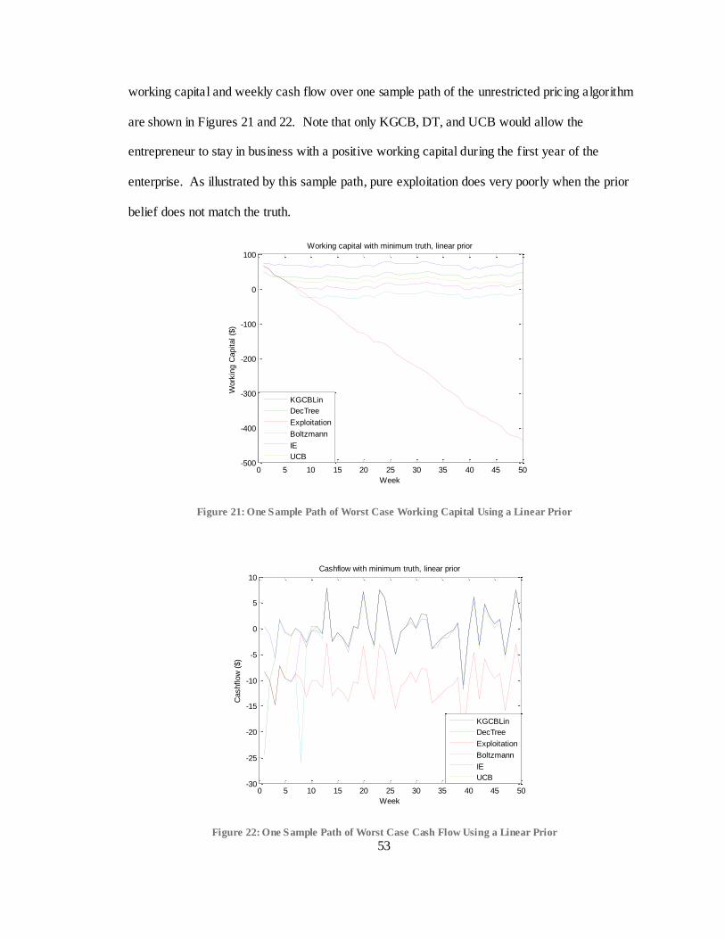
53
working capital and weekly cash flow over one sample path of the unrestricted pricing algorithm
are shown in Figures 21 and 22. Note that only KGCB, DT, and UCB would allow the
entrepreneur to stay in business with a positive working capital during the first year of the
enterprise. As illustrated by this sample path, pure exploitation does very poorly when the prior
belief does not match the truth.
Figure 21: One Sample Path of Worst Case Working Capital Using a Linear Prior
Figure 22: One Sample Path of Worst Case Cash Flow Using a Linear Prior
0 5 10 15 20 25 30 35 40 45 50-500
-400
-300
-200
-100
0
100Working capital with minimum truth, linear prior
Week
Work
ing C
apital ($
)
KGCBLin
DecTree
Exploitation
Boltzmann
IE
UCB
0 5 10 15 20 25 30 35 40 45 50-30
-25
-20
-15
-10
-5
0
5
10Cashflow with minimum truth, linear prior
Week
Cashflow
($)
KGCBLin
DecTree
Exploitation
Boltzmann
IE
UCB

54
For sake of comparison, we use the same random sample path for each policy. That is,
when we observe
, where , we use the same Z observation for
each policy. Each week, of course, we generate a new Z value, but notice that the fluctuations in
the above graph are the same. This stipulation furthermore reduces the size of our confidence
intervals when we later compare policies as it strengthens the basis of comparison.
Figures 21 and 22 show a single sample path of choices, when observations are generated
with noise from the true distribution
. From this single path analysis, we make
two general observations. First, we note that weekly cash flow is highly variable, ranging from
-$25 to $8 under the given policies and making leaps of up to $10 per week, even when
measuring the same prices. In the case with many truths to follow, this variability is hidden
beneath averages. However, in reality, the entrepreneur has one truth and one prior, and his cash
flow variability will likely be closer to that of Figure 22.
Second, we gain insight into specific algorithmic behavior as we examine pricing choices
in Figure 23. Because the policies maximize an online objective, they naturally favor exploitation
over exploration and thus measure prices near $0.25 in early iterations. As the number of
iterations increases, all policies except pure exploitation begin to sample other prices. Although
the KGCB policy finds the optimal price fastest in this case, all the policies except pure
exploitation eventually settle on the optimal price of $0.15. DT’s behavior does not resemble
KGCB’s in this case, despite the fact that they are in the same class of look-ahead policies. By
nature of the prior belief with high variance for each alternative, the extra look-ahead periods bias
DT to choose a higher price than KGCB during the first iteration. After that, DT’s beliefs are
updated and the algorithm steadily moves downward in its choices until it settles on the optimal
price. In contrast, KGCB tends to choose lower prices than the rest of the policies, which is
helpful for this minimal revenue case when the optimal price is low.

55
Figure 23: Algorithm Choices for Worst Case Sample with a Linear Prior
0 5 10 15 20 25 30 35 40 45 50 550
0.1
0.2
0.3
0.4
0.5
KGCB Linear Choices
Week
Price m
easure
d
0 5 10 15 20 25 30 35 40 45 50 550
0.1
0.2
0.3
0.4
0.5
Exploitation Choices
Week
Price m
easure
d
0 5 10 15 20 25 30 35 40 45 50 550
0.1
0.2
0.3
0.4
0.5
Boltzmann Choices
Week
Price m
easure
d
0 5 10 15 20 25 30 35 40 45 50 550
0.1
0.2
0.3
0.4
0.5
Interval Estimation Choices
Week
Price m
easure
d
0 5 10 15 20 25 30 35 40 45 50 550
0.1
0.2
0.3
0.4
0.5
Decision Tree Choices
Week
Price m
easure
d
0 5 10 15 20 25 30 35 40 45 50 550
0.1
0.2
0.3
0.4
0.5
UCB Choices
Week
Price m
easure
d
Figure 23(a): KGCB Choices Figure 23(b): Exploitation Choices
Figure 23(f): UCB Choices Figure 23(e): DT Choices
Figure 23(d): IE Choices Figure 23(c): Boltzmann Choices
56
One reason for the relatively strong performance of all six policies except pure
exploitation is the correlated linear belief updating. After observing a price, the entrepreneur
updates his belief about each of the pricing alternatives in a way that assumes a certain correlation
between each linear parameter. This parameter updating is much more powerful than updating
individual beliefs and greatly aids in the process of finding the optimal price. Also, the
parameters are tuned for the Boltzmann, IE, and UCB policies for each of the different priors to
give optimal results. Because of this, Boltzmann exploration does not look as random and UCB
does not sample as many alternatives as expected, since the tuned parameters bias both policies
towards exploitation.
We omit the restricted pricing results in this case, because the unrestricted choices do not
vary significantly, so the pricing restriction would have a negligible effect.
If the entrepreneur does find himself in the worst case truth where it is very difficult to
make money, his best option is to use a policy besides pure exploitation, and KGCB seems the
best alternative in this sample path. This closely matches reality when an entrepreneur finds that
his intuition is causing him to lose more and more money, and consequently explores prices more
freely. If he can survive his first year, prospects for profitability are high, since in following
weeks the entrepreneur no longer has to pay back $31.20 to the microfinance agency.
5.2 Average Case Policy Comparison with Different Priors
In the average case, the entrepreneur hopes to find the policy that gives maximal profit in
the first year of operation. In the notation introduced in Chapter 3, we denote this policy
optimization as:
(5.1)

57
where is the contribution, or generated profit, from making decision in state . To
simplify notation, we rewrite the expected value in (5.1) as , the profit generated from
using policy given a sample path of observations.
We now give an objective basis for comparison between policies. If we simulate each
policy N times, we can calculate confidence intervals for , the average difference in
profit between policies and according to:
(5.2)
where = ) and the average difference is:
(5.3)
The sample standard deviation for differences is:
(5.4)
The entrepreneur, of course, wants to know if the confidence interval is above or below 0 to
conclude with a high degree of confidence that one policy outperforms the other on average.
We have six primary questions in our average case analysis, each answered by a different
plot in the figures of this section. The questions are summarized as follows:
a. Does KGCB give a more optimal solution than DT? We want to understand whether a
discretized multi-period look-ahead policy with restricted alternatives makes better
decisions than a continuous one-period look-ahead. Because the policies are so similar, it
is illustrative to scrutinize their relative behavior. We give a 95% confidence interval for
the difference between the two policies during each week according to (5.2).
b. Do other polices outperform an entrepreneur’s default strategy of pure exploitation? In
other words, is “typical” human behavior is optimal? We give 95% confidence intervals
for the differences between all other policies and pure exploitation during each week
according to (5.2).

58
c. What is the entrepreneur’s average cash flow in the first fifty weeks of his enterprise?
d. What is the entrepreneur’s average working capital in the first fifty weeks of his
enterprise?
e. How does the entrepreneur’s profit vary with the true maximal revenue? Of course, if
one truth allows the entrepreneur to make higher revenues than another, the former
situation will be more profitable for the entrepreneur. If we eliminate this source of
variability, how do policies compare? Do certain policies perform better in cases when
demand and revenue prospects are lower?
f. If the entrepreneur was to continue his business for a time greater or less than fifty weeks,
how much revenue would he generate? In this analysis, we assume the same micro-loan
payments in each situation for comparison sake. However, in reality, if the entrepreneur
only kept his business open for ten weeks, he would have to make much higher loan
repayments than if he kept his business open for fifty weeks.
We simulate the first five questions over 1000 truths generated from the distribution given in
Chapter 3, and we simulate the last question over 100 truths for N = 5, 10, … 95, 100 weeks.
5.2.1 When the Truth Comes From the Prior Distribution
We first examine the case when the truth comes from a distribution with the same
alternative means as the prior. Unlike an overly optimistic or overly pessimistic prior that
anticipates the same revenue for each price, this prior has a maximum and the entrepreneur has a
clear idea of which price is optimal. However, his belief might not match the true optimum of the
randomly generated truth, so there is some benefit to exploring new alternatives.

59
The results for the unrestricted and restricted analysis are shown on the following two
pages. Because the prior is a very good estimate of the truth, policies find the optimum price
fairly quickly in all cases without wild fluctuations in price choice. As in the worst case truth
with linear prior case, the restricted and unrestricted graphs are almost identical, because the
restriction does not impede any of the algorithms.

60
Figure 24: Truth from Prior, Unrestricted Decisions
0 10 20 30 40 50 60-10
-8
-6
-4
-2
0
2
Week
Diffe
rence in c
ash f
low
KGCBLin vs DecTree
KGCBLin - DecTree
0 10 20 30 40 50 60-10
-8
-6
-4
-2
0
2
Week
Diffe
rence in c
ash f
low
All Policies vs Exploitation
KGCBLin - Exploitation
DecTree - Exploitation
Boltzmann - Exploitation
IE - Exploitation
UCB - Exploitation
0 5 10 15 20 25 30 35 40 45 504
6
8
10
12
14
16
18
Week
Cash f
low
Cash flow over time
KGCBLin
DecTree
Exploitation
Boltzmann
IE
UCB
0 5 10 15 20 25 30 35 40 45 500
100
200
300
400
500
600
700
800
900
Week
Work
ing C
aptial
Working Capital over time
KGCBLin
DecTree
Exploitation
Boltzmann
IE
UCB
30 40 50 60 70 80 90 100-500
0
500
1000
1500
2000
2500
3000
Maximum Revenue
Cum
ula
tive P
rofit
Cumulative Profit as a function of Max Revenue
KGCBLin
DecTree
Exploitation
Boltzmann
IE
UCB
0 10 20 30 40 50 60 70 80 90 1000
200
400
600
800
1000
1200
1400
1600
1800
N (number of weeks)
Avera
ge c
um
ula
tive p
rofit
Average cumulative profit
KGCBLin
DecTree
Exploitation
Boltzmann
IE
UCB
Figure 24(a): KGCB vs. DT Figure 24(b): All policies vs. Exploitation
Figure 24(f): N week profit as fn. of N Figure 24(e): 50 week profit as fn. of max revenue
Figure 24(d): Working Capital Figure 24(c): Cash Flow
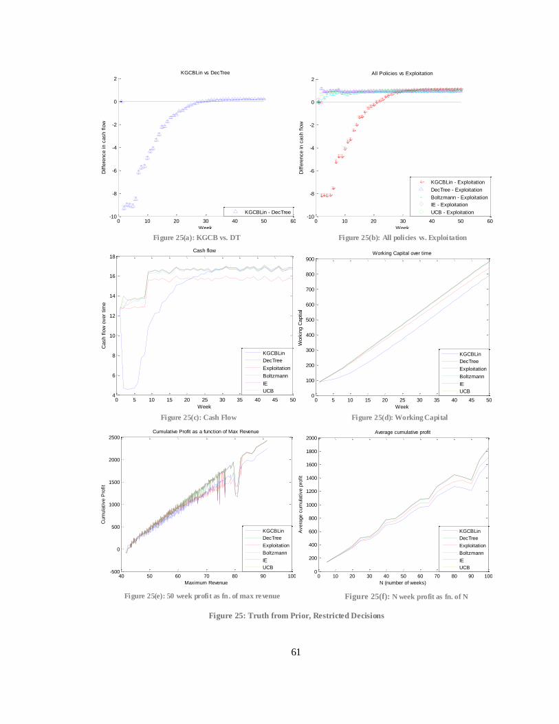
61
Figure 25: Truth from Prior, Restricted Decisions
0 10 20 30 40 50 60-10
-8
-6
-4
-2
0
2
Week
Diffe
rence in c
ash f
low
KGCBLin vs DecTree
KGCBLin - DecTree
0 10 20 30 40 50 60-10
-8
-6
-4
-2
0
2
Week
Diffe
rence in c
ash f
low
All Policies vs Exploitation
KGCBLin - Exploitation
DecTree - Exploitation
Boltzmann - Exploitation
IE - Exploitation
UCB - Exploitation
0 5 10 15 20 25 30 35 40 45 504
6
8
10
12
14
16
18
Week
Cash f
low
over
tim
e
Cash flow
KGCBLin
DecTree
Exploitation
Boltzmann
IE
UCB
0 5 10 15 20 25 30 35 40 45 500
100
200
300
400
500
600
700
800
900
Week
Work
ing C
aptial
Working Capital over time
KGCBLin
DecTree
Exploitation
Boltzmann
IE
UCB
40 50 60 70 80 90 100-500
0
500
1000
1500
2000
2500
Maximum Revenue
Cum
ula
tive P
rofit
Cumulative Profit as a function of Max Revenue
KGCBLin
DecTree
Exploitation
Boltzmann
IE
UCB
0 10 20 30 40 50 60 70 80 90 1000
200
400
600
800
1000
1200
1400
1600
1800
2000
N (number of weeks)
Avera
ge c
um
ula
tive p
rofit
Average cumulative profit
KGCBLin
DecTree
Exploitation
Boltzmann
IE
UCB
Figure 25(a): KGCB vs. DT Figure 25(b): All policies vs. Exploitation
Figure 25(f): N week profit as fn. of N Figure 25(e): 50 week profit as fn. of max revenue
Figure 25(d): Working Capital Figure 25(c): Cash Flow
62
In both the restricted and unrestricted simulations, KGCB’s performance is the worst in
early iterations. As shown in the worst case sample path in the previous section, this is because
KGCB tends to sample lower prices. Because of this propensity, DT makes better decisions than
KGCB in early iterations (Figures 24(a) and 25(a)). However, over time, KGCB’s exploratory
steps pay off and KGCB averages slightly higher revenue than all the other policies. IE,
Boltzmann, and UCB all perform very similarly and very well with a good prior.
Because the prior is very close to the truth, pure exploitation is a fairly good policy.
Although it does not always find the true optimum, its decisions are not so poor in this case, and
its cumulative performance is better than KGCB’s. The other policies, however, still outperform
pure exploitation, even when the truth comes from the prior.
Working capital and cash flow estimates are also high for all policies, as the prior belief
is very good and the entrepreneur finds the optimal price quickly in almost all cases. Over a 50
week period, the entrepreneur can make nearly $900 using value function approximation policies
under our assumptions.
Another notable feature of this particular prior distribution is that there is little variation
in Figures 24(e) and 25(e) which display the cumulative fifty week profit as a function of the
maximum revenue available. This is because the prior is close to the truth and all policies, no
matter what the maximum revenue, have a good general idea of the revenue curve. Thus, they
settle on a fairly good alternative quickly in all cases. When the maximal revenue is low, all
policies accumulate similar revenue; however, as maximum revenue increases, pure exploitation
and KGCB fall behind the rest of the policies. In general, as maximum revenue increases, the
optimal price also increases because when demand increases overall, the entrepreneur can charge
a higher price for a cell phone charge. Since KGCB tends to choose lower prices and pure
exploitation thinks $0.20 is the optimal price in the linear prior case, both policies are penalized
for an increase in the optimal price.

63
No policy performs relatively better with a small number of measurements or a large
number of measurements in Figures 24(f) and 25(f). The more time periods, the more the
behavior of the individual policies is emphasized.
5.2.2 When the Prior is Overly Optimistic
We next examine the situation when the entrepreneur has a very poor prior belief,
thinking that every possible price will yield $80 in revenue per week. In this case, the
entrepreneur has no intuition about the optimal alternative, so the results are likely to be more
varied than in the case where the truth comes from the prior distribution because the early choices
and random observations greatly influence the future belief. Mathematically, for small n,
is more dependent on and x in this case than in the previous case
when the prior was very close to the truth.
First, we give the results for the unrestricted case:

64
Figure 26: Overly Optimistic Prior, Unrestricted Decisions
0 10 20 30 40 50 60-25
-20
-15
-10
-5
0
5
Week
Diffe
rence in c
ash f
low
KGCBLin vs DecTree
KGCBLin - DecTree
0 10 20 30 40 50 60-20
-15
-10
-5
0
5
10
15
20
25
Week
Diffe
rence in c
ash f
low
All Policies vs Exploitation
KGCBLin - Exploitation
DecTree - Exploitation
Boltzmann - Exploitation
IE - Exploitation
UCB - Exploitation
0 5 10 15 20 25 30 35 40 45 50-30
-25
-20
-15
-10
-5
0
5
10
15
Week
Cash f
low
Cash flow over time
KGCBLin
DecTree
Exploitation
Boltzmann
IE
UCB
0 5 10 15 20 25 30 35 40 45 50-300
-200
-100
0
100
200
300
400
500
600
Week
Work
ing C
aptial
Working Capital over time
KGCBLin
DecTree
Exploitation
Boltzmann
IE
UCB
40 50 60 70 80 90 100-500
0
500
1000
1500
2000
2500
3000
Maximum Revenue
Cum
ula
tive P
rofit
Cumulative Profit as a function of Max Revenue
KGCBLin
DecTree
Exploitation
Boltzmann
IE
UCB
0 10 20 30 40 50 60 70 80 90 100-600
-400
-200
0
200
400
600
800
1000
1200
1400
N (number of weeks)
Avera
ge c
um
ula
tive p
rofit
Average cumulative profit
KGCBLin
DecTree
Exploitation
Boltzmann
IE
UCB
Figure 26(a): KGCB vs. DT Figure 26(b): All policies vs. Exploitation
Figure 26(f): N week profit as fn. of N Figure 26(e): 50 week profit as fn. of max revenue
Figure 26(d): Working Capital Figure 26(c): Cash Flow

65
Again, KGCB performs worse than the DT in early iterations because of its tendency to
pick low prices, but after nearly twenty-five iterations KGCB does significantly better than DT
(Figures 26(a) and 26(b)). With this poor prior, we also see the similarities of KGCB and DT
more clearly than in the last case where virtually every policy did well. Especially in Figures
26(c) and 26(f), we observe close behavior of KGCB and DT as the policies settle on close
revenue means, but do not reach the better alternatives discovered by UCB, IE, and Boltzmann.
As the number of weeks in the simulation increases, KGCB and DT also have remarkably similar
performance.
Pure exploitation does very poorly in this case, since the prior is very different from the
truth. As a result, all policies yield much higher revenues and cash flows than pure exploitation
(Figure 26(b)).
With a less accurate prior belief than the previous case when the truth came from the
prior distribution, cash flows and working capital estimates are lower. Instead of making up to
$900 per year, the entrepreneur can only make up to $600 in his first year with the best policies.
As in reality when worse revenue predictions leads to poor decision-making, a bad prior belief
can greatly inhibit profit, even with a good policy.
As predicted, Figure 26(e) with a flat prior shows more variable results than Figure 25(e)
with a curved prior, especially for KGCB. This is because the random observations have greater
effect on future decisions in the case of an overly optimistic flat prior. Because the original prior
is flat, early observations significantly reshape the prior belief on revenue and consequently
induce more varied behavior for different sample paths . From Figure 26(e), it is also clear that
KGCB performs the best for the worst truths, DT performs the best for the best truths, and UCB
performs the best for the average truth from this diagram; possibly a result of KGCB picking
lower prices and DT picking mid- to high-range prices in early iterations of the simulation.
66
For a small number of measurements, DT exhibits the best behavior, but as the number of
measurements increases, UCB leads the other policies in Figure 26(f). One hypothesis for this
result is that UCB explores more in early iterations when we are very uncertain about the
alternative means, because it makes choices depending on which alternatives have not been
measured often. In the case of a flat prior, this is good initial behavior. As the entrepreneur
becomes more certain of which prices are the best, the “bonus factor” of the UCB policy becomes
relatively small and the entrepreneur exploits whatever alternative seems best. Thus, UCB offers
an optimal mix of exploration and exploitation in the case of a flat prior, but also needs a
significant number of iterations to attain this optimal blend. On the other hand, DT performs well
in the beginning by picking mid-range prices because of their high variability. As the number of
iterations increases, DT also begins to exploit its current beliefs because the combination of
observations and the linear belief structure encourages a revenue peak at mid-range prices.
However, because DT begins exploiting too early, as the number of iterations increases, its
performance becomes relatively weaker.
Because policies pick more varied prices in this situation with a flat prior, a pricing
restriction has more notable results than in the previous analysis with a quadratic prior and a clear
maximum. In Figure 27, we repeat the same analysis with a restricted pricing scheme.

67
Figure 27: Overly Optimistic Prior, Restricted Decisions
0 10 20 30 40 50 60-15
-10
-5
0
5
10
15
20
25
30
35
Week
Diffe
rence in c
ash f
low
KGCBLin vs DecTree
KGCBLin - DecTree
0 10 20 30 40 50 60-20
-15
-10
-5
0
5
10
15
20
25
Week
Diffe
rence in c
ash f
low
All Policies vs Exploitation
KGCBLin - Exploitation
DecTree - Exploitation
Boltzmann - Exploitation
IE - Exploitation
UCB - Exploitation
0 5 10 15 20 25 30 35 40 45 50-30
-25
-20
-15
-10
-5
0
5
10
15
Week
Cash f
low
over
tim
e
Cash flow
KGCBLin
DecTree
Exploitation
Boltzmann
IE
UCB
0 5 10 15 20 25 30 35 40 45 50-300
-200
-100
0
100
200
300
400
500
600
700
Week
Work
ing C
aptial
Working Capital over time
KGCBLin
DecTree
Exploitation
Boltzmann
IE
UCB
30 40 50 60 70 80 90 100 110-2000
-1500
-1000
-500
0
500
1000
1500
2000
2500
3000
Maximum Revenue
Cum
ula
tive P
rofit
Cumulative Profit as a function of Max Revenue
KGCBLin
DecTree
Exploitation
Boltzmann
IE
UCB
0 10 20 30 40 50 60 70 80 90 100-600
-400
-200
0
200
400
600
800
1000
1200
1400
N (number of weeks)
Avera
ge c
um
ula
tive p
rofit
Average cumulative profit
KGCBLin
DecTree
Exploitation
Boltzmann
IE
UCB
Figure 27(a): KGCB vs. DT Figure 27(b): All policies vs. Exploitation
Figure 27(f): N week profit as fn. of N Figure 27(e): 50 week profit as fn. of max revenue
Figure 27(d): Working Capital Figure 27(c): Cash Flow

68
All policies are more volatile with the restricted pricing scheme, but most of the general
behavior is the same as that of Figure 26 with the unrestricted prices. Relative behavior of
policies as well as the magnitude of cash flow and working capital estimates is the same, so we
only discuss the effect of increased volatility in price choices.
Each of the policies gives more variable average cash flow and working capital (Figures
27(c) and 27(d)) in early iterations using the restricted pricing scheme and furthermore takes
slightly longer to reach a steady revenue stream. This is because restricted pricing constrains the
entrepreneur to move his price slowly from week to week and thus forces more measurements of
poor alternatives in early iterations if the first revenue measurement was particularly low.
However, this also has long term benefits, as the entrepreneur on average reaches a higher
revenue stream than in the unrestricted case (compare Figures 27(c) and 26(c)). Just as the
KGCB algorithm generally samples more poor alternatives than DT in early iterations and later
outperforms DT because of the perspective gained by the initial exploration, so the entrepreneur
with restricted prices reaches a more optimal revenue in the long run than in the unrestricted case.
Figures 26(e) and 27(e) show that in the unrestricted case, KGCB demonstrates the most
volatile behavior, while in the restricted case, DT exhibits the most variation in cumulative profit.
One possible explanation for this occurrence is that the pricing restriction has more influence with
more look-ahead periods. That is, with a pricing restriction, DT’s initial prices are highly
dependent on the revenue observation in the first week, as this determines whether DT should
pick a higher or lower price in the following week. This decision impacts all future decisions,
and thus one random observation has great influence on the performance of the algorithm.
KGCB’s behavior is not as volatile with the restricted pricing scheme because KGCB does not
anticipate price restrictions in its algorithm.

69
5.2.3 Value Function Approximation vs. Look-ahead Policies
From this analysis, it appears that the value function approximation policies outperform
the look-ahead policies with good (truth) and bad (overly optimistic) priors on average. This is
perhaps counterintuitive, since the look-ahead policies are more mathematically complex as they
project into the future and use more sophisticated algorithms to make a decision. We then come
to the age old question - whether more complex processes necessarily imply better results.
However, the question is not as obvious as stated above. The “hard” part of KGCB and
DT is the looking forward and taking expectations of future rewards. The “hard” part of interval
estimation, Boltzmann exploration, and upper confidence bounding is the tuning of parameters to
yield optimal results. Without properly tuned parameters, all three policies can result in
arbitrarily poor performance. Thus, in practice the value function approximation policies are
much harder to implement, since we must have some notion of the truth distribution to adequately
simulate scenarios and pick the best parameters for each prior case. KGCB and DT, on the other
hand, require more computational power to calculate expectations, but are not contingent on a
parameter for their results.
Also, from the analysis of this chapter, it appears that an entrepreneur can make between
$10 and $18 per week on average in addition to his $10 weekly salary. These figures also include
loan payments, so after the first year of paying back his loan, the entrepreneur could make $40 to
$48 profits which are impressive in Africa. However, because of all the assumptions listed in
Chapter 2, we caution the reader to view the numerical results in this chapter not as definitive, but
rather as illustrative of a decision-making process and finding an optimal policy. Though profits
are also important, the numbers here are not as important as the methodology.

70
CHAPTER 6 Business Considerations
A successful business is not merely a product of rosy financial projections and optimal
pricing algorithms; it is rather the unity of an important problem and a viable solution in a
favorable context. In this chapter, we seek to shed light on the non-financial aspects of a solar
mobile charging enterprise using the framework of William Sahlman of Harvard Business School
(1999). Sahlman states that the primary “dynamic components” of the entrepreneurial process are
the people, opportunity, external context, and financial deal. Together, these four aspects paint a
vivid picture for the prospects of an actual business founded upon the principles already
mentioned in this thesis.
We begin with an evaluation using the four concepts proposed by Sahlman and conclude
with two case studies of actual solar charging businesses that have been formed on similar
concepts; one a formal NGO and the other an informal entrepreneurial venture. Together with the
more narrow scope of the previous chapters, this analysis gives a more balanced view of the
entrepreneurial process and shares insight from real solar efforts in Africa.

71
6.1 People: Who is involved
Venture capitalists often say they invest in people, not ideas. Any number of factors can
prevent a technology from succeeding, but even the best technology will not go to market with
the wrong entrepreneur handling day to day business. The primary quality in the ideal
entrepreneur to run this solar cell charging business is not necessarily experience or technical
expertise, but rather, creative adaptability. Because many factors are highly variable in this
scheme – the number of customers, the hours of sunlight, customer expectations – an
entrepreneur must be flexible in his dealings with customers. When a customer tries to negotiate
a charging price down to half in typical African fashion, the entrepreneur must strike a balance
between the customer’s expectations and his own. During a week of cloudy days, he must
prioritize which customers really need their cell phones charged at any given time and turn the
rest away to other vendors. When cash starts to run out, he must consider whether to move his
business to another area with higher demand or ask for more funding. When the competitor with
a battery on a bike starts undercutting his pricing scheme, he must be ready to retain customers in
another fashion; perhaps promote his business as safer for the user’s cell phone , run a special
charging deal for a week, or even allow customers to watch TV while their phones are charging.
To gain a substantial market share quickly, it is also imperative that the entrepreneur has
local connections. Personal ties cannot be understated in African culture and people consequently
often charge their phones with their friends or relatives. A successful entrepreneur, then, must be
familiar with his market and his market must be familiar with him.
Finally, an entrepreneur must be committed to this project as more than simply a money-
making business, although it will hopefully also be that. He must carry the vision of solar power
changing Africa and communicate this to his clients, allowing them to share a breakthrough
technology that will eventually revolutionize their way of life. In this way, people are attracted to
his business not only for its superior cost, but also for its excit ing and transformative prospects.

72
Looking ahead towards a larger goal, the entrepreneur is also motivated to continue in his
business even during rough periods with panel break-downs, lack of customers, or unanticipated
change in demand.
6.2 Opportunity: Customer, Market, and Competition
When evaluating potential opportunity in a business, broad market analysis is essential.
We first think realistically about the target customer’s needs and wants, and then proceed to
assess what structural aspects make the market easy or difficult to penetrate. To gain a further
understanding of how an entrepreneur can add and protect value in his enterprise, we lastly
provide a brief comparative cost analysis between solar and other charging options.
There are two potential customers for the solar mobile charging station. The first is the
individual cell phone user on whom we have focused most of the analysis thus far. Without
another source of electricity, an individual user charges his phone at the entrepreneur’s station for
a small fee. This user is highly sensitive to price, personal relationship with the entrepreneur, and
ability to charge other appliances.
The second less obvious customer that the entrepreneur should consider is a mobile
network operator. Since making a charging solution widely available has great potential to
increase an operator’s revenues, it is in the operator’s best interest to provide a low-cost charging
solution to allow users to talk more freely on their phones. An entrepreneur might also be able to
set up a deal with a local network operator wherein the latter subsidizes the charging station so
the former can undercut competing prices. The operator would allow the entrepreneur to keep
most of the charging profits and would make its pr imary revenue through increased air time from
customers. This arrangement is beneficial for both parties. With little investment besides cash,
the operator builds a green reputation by subsidizing a solar power solution in addition to a
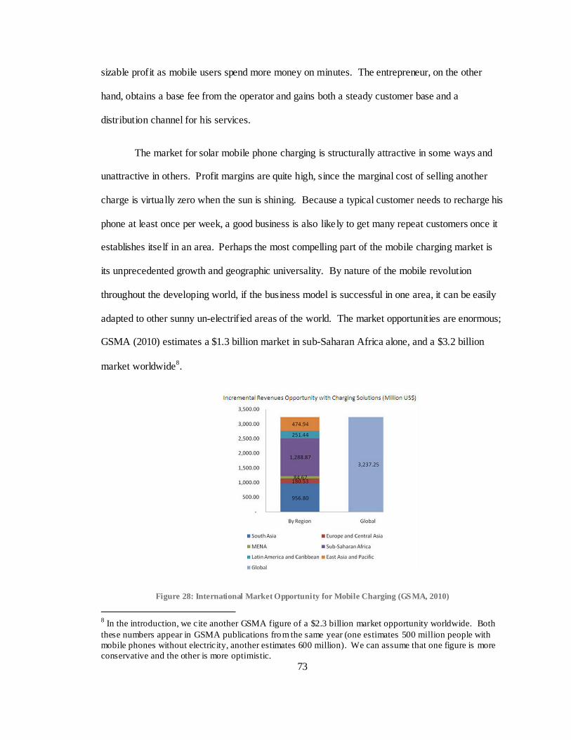
73
sizable profit as mobile users spend more money on minutes. The entrepreneur, on the other
hand, obtains a base fee from the operator and gains both a steady customer base and a
distribution channel for his services.
The market for solar mobile phone charging is structurally attractive in some ways and
unattractive in others. Profit margins are quite high, since the marginal cost of selling another
charge is virtually zero when the sun is shining. Because a typical customer needs to recharge his
phone at least once per week, a good business is also likely to get many repeat customers once it
establishes itself in an area. Perhaps the most compelling part of the mobile charging market is
its unprecedented growth and geographic universality. By nature of the mobile revolution
throughout the developing world, if the business model is successful in one area, it can be easily
adapted to other sunny un-electrified areas of the world. The market opportunities are enormous;
GSMA (2010) estimates a $1.3 billion market in sub-Saharan Africa alone, and a $3.2 billion
market worldwide8.
Figure 28: International Market Opportunity for Mobile Charging (GSMA, 2010)
8 In the introduction, we cite another GSMA figure of a $2.3 billion market opportunity worldwide. Both
these numbers appear in GSMA publications from the same year (one estimates 500 million people with
mobile phones without electricity, another estimates 600 million). We can assume that one figure is more
conservative and the other is more optimistic.
74
Another favorable aspect of this enterprise is that the entrepreneur’s initial investment in
solar modules and related equipment is not restricted to mobile charging. If the entrepreneur
finds that cell phone charging is not in as high demand as he originally suspected, he can
purchase an inverter at fairly low cost and also allow customers to charge other appliances,
particularly lights and lamps. Though pricing schemes for such an operation are not mentioned in
this thesis, they could be derived in a similar fashion to the analysis in Chapters 2 and 3 as the
entrepreneur builds up a prior belief regarding the demand curve for other devices. This
versatility makes solar a particularly good investment.
The barrier to entry in the solar charging market is not unequivocally high or low. In
argument of a low barrier, initial capital costs just over $1000 are not so high that a fairly wealthy
local could not purchase his own solar panels and start his own business. It seems that only cash
or other financing options prohibit others from entering this fairly simple market. However,
considering that rich locals must have some other source of income to account for their wealth, it
is unlikely that they would have the time, desire, or commitment to invest in a start-up.
Furthermore, a relatively poor entrepreneur has a greater likelihood of succeeding in this industry
since he knows how to be frugal in his expenses and he knows more potential customers
personally, as a community’s lack of electricity tends to be highly related to poverty. Local
contacts, procurement of initial investment, and a commitment to protect and maintain solar
equipment consequently raise the barrier for other entrepreneurs to enter this industry.
From the perspective of a poor entrepreneur, the most unattractive aspects of the mobile
charging market are the high capital costs, high risk, and strong competition resulting from the
commodity nature of mobile charging. If an entrepreneur finds himself in an area where the he
simply cannot make enough profit to sustain himself because the market is too small or people are
unwilling to try a new technology, he has lost a great deal of cash. Though he can salvage his

75
costs by charging other products or selling his modules to a willing buyer, heavily front-loaded
costs are generally bad from a business perspective because the entrepreneur has more at stake in
the early stages of his enterprise.
Because a cell phone charge is a commodity good, only differentiated by price in most
customers’ minds, the entrepreneur has to introduce a new way to protect value in his enterprise
besides cost-competitiveness. In the African context, this value protection can be personal
customer ties, a reputation for quality charging, or versatility in other services.
In commodity markets, competition is generally fierce and cell phone charging is no
different. Competition from other off-grid sources can be strong in these emerging markets,
mostly from portable car batteries and diesel generators. Besides the obvious advantage that
equatorial Africa receives high-intensity sunlight for many hours each day, solar, however, does
possess significant quantitative and qualitative advantages over these two competitors. Solar
energy requires no additional fuel, can be easily scaled upwards by adding additional panels, and
calls for little day-to-day maintenance. In remote rural areas, the initial cost of a diesel generator
($0.65 per watt) is much lower than that of a solar system ($5 per watt), especially with the
purchase of a used generator. Despite early savings, the time and monetary costs of obtaining
fuel and performing oil and filter change maintenance quickly add up. Solar, on the other hand,
has a higher initial cost, but negligible operating cost.
Batteries are a popular option for cell charging entrepreneurs, because of the low initial
cost and portability. In the short term, when the rapidly changing environment makes
entrepreneurs fearful of longer term investments, a battery is a good choice. However, while this
current practice of charging a car battery in town and then selling the power to neighbors is most
pervasive at present, high operating costs to repeatedly charge the battery from a third party and
short battery lifetimes yield significant expenses over time. Though batteries under ideal
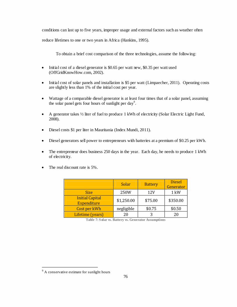
76
conditions can last up to five years, improper usage and external factors such as weather often
reduce lifetimes to one or two years in Africa (Hankins, 1995).
To obtain a brief cost comparison of the three technologies, assume the following:
Initial cost of a diesel generator is $0.65 per watt new, $0.35 per watt used (OffGridKnowHow.com, 2002).
Initial cost of solar panels and installation is $5 per watt (Limpaecher, 2011). Operating costs are slightly less than 1% of the initial cost per year.
Wattage of a comparable diesel generator is at least four times that of a solar panel, assuming the solar panel gets four hours of sunlight per day
9.
A generator takes ½ liter of fuel to produce 1 kWh of electricity (Solar Electric Light Fund, 2008).
Diesel costs $1 per liter in Mauritania (Index Mundi, 2011).
Diesel generators sell power to entrepreneurs with batteries at a premium of $0.25 per kWh.
The entrepreneur does business 250 days in the year. Each day, he needs to produce 1 kWh of electricity.
The real discount rate is 5%.
Solar Battery Diesel
Generator
Size 250W 12V 1 kW
Initial Capital Expenditure
$1,250.00 $75.00 $350.00
Cost per kWh negligible $0.75 $0.50
Lifetime (years) 20 3 20 Table 7: Solar vs. Battery vs. Generator Assumptions
9 A conservative estimate for sunlight hours

77
YEAR Solar CD10 Solar
Battery CD
Battery Diesel
Generator CD
Generator
0 $1,250.00 $1,250.00 $262.50 $262.50 $350.00 $350.00
1 $10.00 $1,259.52 $187.50 $441.07 $125.00 $469.05
2 $10.00 $1,268.59 $187.50 $611.14 $125.00 $582.43
3 $10.00 $1,277.23 $262.50 $837.90 $125.00 $690.41
4 $10.00 $1,285.46 $187.50 $992.15 $125.00 $793.24
5 $10.00 $1,293.29 $187.50 $1,139.06 $125.00 $891.18
6 $10.00 $1,300.76 $262.50 $1,334.95 $125.00 $984.46
7 $10.00 $1,307.86 $187.50 $1,468.20 $125.00 $1,073.30
8 $10.00 $1,314.63 $187.50 $1,595.11 $125.00 $1,157.90
9 $10.00 $1,321.08 $262.50 $1,764.32 $125.00 $1,238.48
10 $10.00 $1,327.22 $187.50 $1,879.42 $125.00 $1,315.22
11 $10.00 $1,333.06 $187.50 $1,989.05 $125.00 $1,388.30
12 $10.00 $1,338.63 $262.50 $2,135.22 $125.00 $1,457.91
13 $10.00 $1,343.94 $187.50 $2,234.66 $125.00 $1,524.20
14 $10.00 $1,348.99 $187.50 $2,329.36 $125.00 $1,587.33
15 $10.00 $1,353.80 $262.50 $2,455.62 $125.00 $1,647.46
16 $10.00 $1,358.38 $187.50 $2,541.52 $125.00 $1,704.72
17 $10.00 $1,362.74 $187.50 $2,623.33 $125.00 $1,759.26
18 $10.00 $1,366.90 $262.50 $2,732.40 $125.00 $1,811.20
19 $10.00 $1,370.85 $187.50 $2,806.60 $125.00 $1,860.67
20 $10.00 $1,374.62 $187.50 $2,877.27 $125.00 $1,907.78 Table 8: Solar vs. Battery vs. Generator Comparison
The highlighted portions of the chart show that in this simplified analysis, solar is more
cost-effective than a lead-acid battery after six years and more cost-effective than a diesel
generator after eleven years. Over time, the solar entrepreneur’s profit margins are higher than
his competitors and he can offer lower prices. In the short-term, however, if an entrepreneur
hopes to ride the wave of cell phone charging demand, a battery is the best option.
As a long-term investment, solar equipment is a worthwhile purchase. The entrepreneur
must first find a feasible market with a clear demand for mobile charging or with a viable
network operator partner. In a highly uniform industry where cell phone charging is a commodity,
he must think of ways to protect value in his enterprise by offering superior prices or additional
10
CD refers to the cumulative discounted cost

78
services for his customers. If the charging market evaporates suddenly with the introduction of a
large electricity provider, the entrepreneur must adapt to the changing environment and diversify
his offerings accordingly or in extreme circumstances, sell his panels and seek another area to
establish the same type of business.
6.3 Context: African Entrepreneurship
Starting a business in Africa is quite a different experience than starting a business in
America. In a study on “Ethnic Entrepreneurship”, Mitchell of South Africa’s University of
Natal states that financing, labor regulations, crime, and theft are the most problematic practical
policy aspects to African new businesses establishment (2003). Perhaps the most unusual barrier
to African entrepreneurship is a sector of customers quick to vandalize, steal, and criticize new
technology. An entrepreneur has to be especially wary of theft when he carries expensive pieces
of equipment such as solar modules that can be pawned for cash. Numerous horror stories detail
the potential dangers of starting a business in Africa: angry customers who destroyed a generator
after the power went off for a night, vandals who clipped wires to protest rising electricity prices,
unofficial customers who hacked the grid connection to add a wire to their own home for free
electricity access (Limpaecher, 2011).
The IFC and World Bank ranked Mauritania 152 out of 183 world economies in the ease
of starting a business (2011). The most apparent reason for the low rating is that Mauritania
requires an entrepreneur to deposit slightly under $4000 in a bank or notary before registration
and up to three months after incorporation. Though this paid-in capital figure is not high
objectively, it relatively represents 412% of Mauritania’s GNI (gross national income) per capita,
most likely a result of a weak banking system coupled with a fear of bad start-ups. However,
these metrics are for small to medium start-ups funded by traditional loans from banks; so the

79
entrepreneur could hopefully avoid some of the regulations by obtaining a microfinance loan or a
personal loan from friends.
6.4 Deal: Financing Decisions
Assuming the entrepreneur has little or no cash of his own, there are three primary
options for the entrepreneur to fund his initial capital expenditures. The entrepreneur can pay for
his solar module and other equipment via a loan from friends and family, a bank, or a
microfinance institution. A loan from family or friends is certainly the most flexible option, but
the entrepreneur does not receive the same advice, training, and accountability he would obtain
from a microfinance institution. If the entrepreneur takes a loan from personal friends, he also
has more at stake than just monetary investment in his company. If he fails to provide a positive
return on his friends’ investment, he also jeopardizes their welfare and possibly their relationship.
Compared to a microfinance institution, the entrepreneur may save on interest payments
with a commercial bank. Nevertheless, there are unfortunately other drawbacks besides even
outrageously high paid-in minimum capital laws. Because there are only ten commercial banks
in all of Mauritania according to the Consultative Group to Assist the Poor (2011), obtaining a
loan may be near-impossible if the entrepreneur has little credit history. As only 0.1% of
Mauritanian adults have data in the past five years listed the public credit registry (World Bank &
IFC, 2011), it is extremely difficult to take out a loan. Even if the entrepreneur is able to procure
credit, his legal rights are minimal should the lending institution declare bankruptcy.
With a microfinance institution, the entrepreneur receives business training and support,
but also must pay back his loan with high interest on a very strict schedule. Though the regular
check-ups and loan repayments encourage the entrepreneur to be disciplined about making his
business thrive quickly, these additional responsibilities from the lending institution make

80
microfinance loans especially expensive to disburse. As a result, interest rates on microfinance
loans are notoriously high.
We summarize the important aspects of the different financing options below. One way
to view Table 9 is that the financing structures are arranged from top to bottom as the most to
least preferable, but also the most to least difficult to obtain. A personal loan, or even better, a
business founded entirely from personal savings requires the entrepreneur to pay back little or no
interest on a loose schedule. A bank loan offers medium interest rates conditional on the
entrepreneur’s credit history, while a microfinance institution offers the highest interest rates, but
also can provide loans to poor entrepreneurs with little financial history.
Interest Rate Time to pay back
loan
Loan from family/friends
0%-10%11 indefinite12
Loan from bank 10-30%13 1-5 years14
Loan from microfinance lender
30-40%15 1-2 years16
Table 9: Loan Options
Yet, interest rates should not be the only deciding factor in the entrepreneur’s decision.
There is also something to be said for the work ethic and discipline that comes with managing
someone else’s money and staying on a predictable schedule. Because of this, the entrepreneur
should think carefully through the options given his past experience running a business and his
current personal financial situation.
11
Estimated 12
Estimated 13
Estimated; bank lending rates were unavailab le 14
Estimated 15
KIVA, 2011 16
Field & Pande, 2007

81
6.5 Two Case Studies
It is difficult to imagine the potential successes and downfalls of a solar business in
Africa without concrete examples. We now draw lessons from two African enterprises that have
successfully sold electricity to locals using solar panels. The first is a local entrepreneur in
Mauritania and the second is a large NGO in West Africa.
6.5.1 Bababé Entrepreneur
Although reality is never as exact as numerical assumptions, it is promising to see that
actual entrepreneurs have undertaken similar small-scale solar enterprises in recent years. In
1991, a local entrepreneur in Bababé, Mauritania, Abdoulaye Ba, bought two solar panels for
approximately $180 (USD) each to light his home with renewable energy. The panels had the
capacity to run five lights or three lights and a TV. Ba began an unofficial movie theater business,
charging locals to watch soccer games from his television.
As cell phones became more and more prevalent, neighbors demanded a paid charging
service in 2005. In response, Ba added two larger solar panels to his existing modules for $400
(USD) each. On average, ten customers came to Ba each day to charge their phones for $0.20
each. With a burgeoning cell phone market and a stagnant electricity supply, it was the ideal time
to start a charging business in Bababé. From rudimentary supply and demand, we know that
when demand shifts outward from to and supply remains the same, equilibrium price and
quantity both increase, as in Figure 29(a). Thus, when Ba later increased the price per charge to
$0.40, he actually had more customers than in early stages of the business as a result of the sharp
increase in demand for electricity.

82
Figure 29: Changes in Demand and Supply in the Market for Cell Phone Charging
Recently, large electrification advances were made in Bababé, and the supply for cell
phone charging increased from to in Figure 29(b). As a result, equilibrium quantity rose,
but price fell from to . Because Ba did not solely depend on the charging business for his
income, he was not as intent on finding the profit maximizing price as the hypothetical
entrepreneur presented in the thesis, and he continued to charge the same $0.40 per phone. As
expected, demand consequently dropped to only five customers from remote villages per month.
Over time as the business became less profitable, Ba sold all but one of the panels for roughly
half of the original purchase price. Today, he keeps his remaining panel to light his home and run
his makeshift movie theater.
As illustrated by Ba’s experiences, a business-savvy entrepreneur must be highly aware
of changing infrastructure and changing consumer tastes. Supply and demand can shift at any
time based on the actions of the government, a network operator, or a nearby NGO. We can
capture this in our simulation model by using non-stationary demand and supply distributions,
wherein the true demand and supply change week by week with or without a general trend.
However, the actual dynamics of an expanded cell phone network or the advent of electricity in a
community are very difficult to predict mathematically. It is often better to adapt according to the
Figure 29(a): Increased Demand Figure 29(b): Increased Supply

83
information one gathers day by day than to err on the overly cautious side by accounting for a
shifts in supply and demand during every time period.
The greatest threat to the cell phone charging business is a shift in electricity supply.
With a new generator in town or a new series of wires strung from a nearby village, villagers can
purchase the electricity needed to charge a phone for a few cents. A business founded upon cell
phone charging is then obsolete unless the entrepreneur can make some quick changes. He has at
least two options: first, to terminate the business and sell the solar panels and second, to tweak his
business to offer a different service such as charging batteries for lanterns. Ba did a combination
of the two. Note, however, that by 2009 estimates, 85.7% of rural sub-Saharan Africa still live
without access to electricity (IEA), and even with the UN’s Millennium Development Goal to
eradicate extreme hunger and poverty by 2015 by providing electricity to 395 million people
worldwide, gaping infrastructure needs will still leave the majority without electricity. Thus, this
need for cell phone charging is not likely to be eliminated completely in the near future.
It is also important to consider the benefit of diversifying service offerings to protect
against such a market shift in supply. Ba charged batteries and ran a TV for profit in addition to
charging cell phones. Each of these offerings has a different consumer base and a different
barrier to entry. While businessmen and young people are the primary customers for cell phone
charging, TV services appeal to the non-working sector during the day and virtually everyone in
the evening. Lighting needs are also universal. Because running a television or charging a
battery requires more energy than charging a cell phone, it is more difficult for another
entrepreneur to offer the same service. Furthermore, a TV is another high initial cost that
prevents others from running a home movie theater. In contrast, there is not considerable
distinction in the cell phone charging market; as long as the battery is charged properly,
customers get the same service with any entrepreneur. A movie theater, on the other hand, has
84
more opportunity for the entrepreneur to offer superior service by providing concessions,
showing the most exciting soccer matches, or attracting the biggest crowd.
6.5.2 Energy For Opportunity
Specializing in small scale solar installation, Energy For Opportunity (EFO) was founded
in 2009 by two social entrepreneurs passionate about spreading solar throughout West Africa.
Simon Willans and Paul Munro first met while working on renewable energy projects in Sierra
Leone, Liberia, and Uganda and now focus on a holistic approach to renewable energy adoption
in Benin, Mali, and Sierra Leone, eventually hoping to expand services throughout West Africa.
While many organizations are focused strictly on installing solar panels, EFO takes a longer term
attitude, training students to use solar technology in conjunction with local schools and
encouraging government and international offices to adopt solar as well.
EFO’s four primary areas of focus are Skills Training, Development and Livelihoods,
Education, and Health. Their current Development and Livelihoods project is a community
charging initiative in which they hope to establish ten solar stations in Benin and then transfer
ownership to trained members of the community. Although EFO provides initial funding, they
seek to build self-sustaining enterprises that not only generate profit for the local owners of the
stations, but also reduce dependence on kerosene and batteries in the communities. EFO is more
than just a solar-focused micro-finance lending institution; the organization procures initial
equipment and provides complete training for the entrepreneur in business management and solar
maintenance. Because EFO already has contacts in communities, they are able to tailor
community charging applications specifically for local needs; allowing a particular focus on
lighting, cell phone charging, radios, or the most imminent and popular appliances. EFO seeks to
raise $100,000 for this project, which is considerably more than our estimates for ten individual
mobile charging enterprises because of the greater capacity and wider range of services provided.
85
Since EFO is a non-profit organization funded primarily by grants and contracts, it is not
as dependent on revenue streams as an individual entrepreneur’s business. Only 2% of their total
revenue in 2009-2010 came from sales, because most of the emphasis was on contract jobs for
hospitals and government buildings rather than on projects that brought direct revenue from
consumers. EFO’s first year of operation is certainly not representative of the future of the
company, however, it nonetheless illustrates the general principle that a non-profit has
significantly different objectives and much more flexible funding than an individual entrepreneur.
Although we have focused primarily on a small-scale for-profit business thus far, it is
helpful to also consider the option of a more broad non-profit founded upon the same principles.
A large non-profit has the capacity to engage more in-depth in communities, work toward long-
term change in attitudes towards renewable energy, and obtain funds from governments and
donors. Optimal pricing is not as important in this context, since the chief goal is not profit, but
rather long-term introduction of renewable energy in developing communities.

86
CHAPTER 7 Conclusion
Opportunity creation is the goal of modern innovation. Cell phones create opportunity
for the users by increasing communication efficiency and eliminating third party intervention in
commerce and banking. Solar creates opportunity for a developing nation by allowing villages to
meet small electrification needs with micro-grids rather than wait for a big electricity company to
expand the grid where infrastructure is lacking. A solar cell phone charging business creates
opportunity for an entrepreneur by providing personal profit and business development while
simultaneously promoting the positive externalities of both cell phones and solar power in the
community.
The goal of this thesis was to maximize the opportunity created by a solar micro-grid
charging enterprise. We obtained not only numerical estimates of profit in different scenarios,
but also established a general structure guiding the entrepreneur’s decision making process from
the creation of the prior belief to policy optimization to real business considerations. In reality,
most decisions are made with fairly simple policies that mix exploration and exploitation
according to the decision maker’s self-confidence and risk-aversion. However, in an increasingly
technological world where more and more “easy” decisions are being made by computers, it is
instructive to see how well selection algorithms compare to human intuition and to one another.

87
With this analysis, we understand the pros and cons of various policies in a diverse range of
scenarios.
7.1 Main Findings
From basic cost-revenue analysis, we learned that mobile charging is a highly lucrative
market with significant unmet demand. Even in our most conservative analysis, with the right
policy, the entrepreneur can make profits in the first year of his enterprise while still paying off
his initial loan.
In the worst case analysis where the entrepreneur received minimal revenue each week,
KGCB and DT performed slightly above the other policies. Pure exploitation, of course, behaved
the worst because revenues in the truth were lower than revenues in the prior.
For a good prior which closely resembled the truth, all policies performed well without
much variation over many truths. With the exception of pure exploitation which continued to
sample the same alternative even with belief-updating, all policies found optimal or near-optimal
alternatives fairly quickly. KGCB had a tendency to pick lower prices in early iterations, which
affected its initial performance negatively.
For a bad prior which assumed all prices yielded the same revenue, the entrepreneur’s
average profit was significantly lower than average profit with a good prior, most notably in early
iterations of the algorithm. Out of all the policies, pure exploitation suffered the most with a bad
prior. Just as in reality, one should not strictly follow intuition, so in our model, we learned that
over many truth possibilities, pure exploitation is a poor policy.
The restricted pricing scheme had the most effect in the bad prior case when choices were
naturally more volatile as the entrepreneur’s intuition was incorrect. Restrictions increased the
number of iterations needed to find the optimal price for nearly all policies and also introduced

88
higher variability to DT, which projected restrictions into the future and was subsequently highly
dependent on the first few sample observations.
In the average case analysis over many truths, UCB performed the best with all four
priors tested, but most significantly for priors that were overly optimistic or pessimistic. While
the policies with tunable parameters slightly outperformed the look-ahead policies for bad priors,
they also required tuning for each possible prior, which assumed foreknowledge of the truth
distribution. If an entrepreneur was to actually enter an area with a poor prior and a poor tunable
parameter, the look-ahead policies would certainly outperform the tunable policies.
From a business perspective, it is best to broaden notions of the customer market and also
consider deals directly with mobile network operators or existing cell phone companies. Solar
has great potential in Africa, but its success in the cell phone charging industry is highly
contingent on finding the right entrepreneurs who are adaptable to the rapidly changing
environment. The same swift evolution that makes revenue projections so unpredictable and
consequently introduces immense uncertainty for an investor also creates a wealth of unexplored
market opportunities for entrepreneurs.
7.2 Assumptions Revisited and Future Research
As illuminated by the strictly business analysis of Chapter 6, the most unrealistic
assumption in our model was that the entrepreneur only meets one type of demand with his solar
panels. Both business models in the case studies diversif ied offerings to hedge against the
possibility of a steep increase in electricity supply or a new cell phone technology that eliminates
the need for traditional charging. Although this assumption of only meeting cell phone charging
demand lent to a more reliable prior belief as the number of variables and estimation quantities
were minimized, it also restricted the entrepreneur’s ability to enter other markets.
89
However, this assumption is not as impractical as it may seem. Our mathematical model
was never meant to be taken as a holistic business plan, but rather, as a framework to examine a
particular type of decision making process. If unmet cell phone charging demand is high enough,
a specialty charging shop that only charges cell phones could be very successful for a short period
of time. When new entrepreneurs jump into the market or the village gains access to a new large-
scale generator or charging station, the entrepreneur then has enough capital to purchase extra
inverters and batteries to offer unique services such as TV or even refrigeration. He can perform
the same analysis to build up a prior belief and use a policy to make pricing decisions in the new
market as well.
Throughout our model, we also assumed that the entrepreneur could change price freely
from week to week. Though we partially remedied this vast simplification by introducing a
restricted decision set in all the policies, there are other ways we could further refine this
assumption and reflect it accurately in our model. Future research could either re-derive all the
policies to restrict pricing sets or account for user pricing psychology by introducing some
penalty factor for changing price by a large amount. True demand could be a non-stationary
function of the change in last week’s price to this week’s price, such that angry customers would
avoid a business if it sharply increased the price from last week or grateful customers would
return if the business sharply decreased the price from last week. If DT was modified to reflect
this non-stationary assumption, it would most likely outperform the other policies as it would
possess the ability anticipate a future reward from gradually decreasing one’s price.
Practically, the most imminent future topic of research regarding this business is actual
field data. Although data for costs and revenues were gathered as averages through online
sources and a few local contacts, it is likely that government subsidies or socially conscious
suppliers might offer discounts that would drive down the high initial cost of solar panels in
Africa. Concerning demand estimates, nothing can compare to the experience of actually starting

90
such a business and viewing the consumer market firsthand. From a simulation window, we only
see demands, revenues and costs; from a ground perspective, we see the real charging needs of
people and the tangible change that cell phones bring to rural communities.
There are many other questions proposed in this model that could be examined in a
rigorous mathematical framework. We could solve for an optimal stopping policy for the
entrepreneur. After how many weeks of consistently low revenue should the entrepreneur decide
that his best option is to either fold the business or move to another location? If customers arrive
faster than they can be serviced, we could calculate queuing statistics such as the average wait
time in line for a customer, or the utilization rate of the entrepreneur’s charging outlets. These
are only a few of the other approaches one could take to this problem.
7.3 Final Thoughts
A solar mobile charging system in Africa has potential not only to facilitate the adoption
of a clean renewable energy source to a developing continent, but also to bring profit to the
entrepreneur himself. Though starting a new enterprise is a multi-faceted undertaking whose
success is contingent on both exogenous and endogenous factors to the entrepreneur, by
providing policies for the optimal pricing problem, we give the reader a taste of one of the many
challenges in entering an emerging market such as this. With a policy that creates a metric to
evaluate price alternatives besides just their expected revenue, the entrepreneur has a high
likelihood of finding the profit-maximizing price. Though tunable policies performed best in
simulation, look-ahead policies are easier to implement in reality.
Neither cell phones nor solar technology are Africa’s “silver bullet” of development.
However, by continually thinking of new ways to use cell phones to practically bridge

91
communication gaps and inefficiencies, and by slowly introducing solar as a viable energy
source, we stand at the cusp of a an exciting epoch in world history.

92
WORKS CITED
"African Mobile Subscriber Growth and Penetration, 1998-2010." Africa & The Middle East Telecom 11.3 (2010). January 22, 2011.
Aker, Jenny C. and Issac M. Mbiti. "Africa Calling: Can Mobile Phones make a Miracle?" Boston
Review, March/April 2010. October 12, 2010. Auer, P., Cesa-Bianchi, N. & Fischer, P. "Finite-Time Analysis of the Multiarmed Bandit
Problem." Machine Learning 47.2-3 (2002): 235,235-256. Ba, Ibrahima. Personal Communication, 2011. Breiman, L., J. H. Friedman, R. A. Olshen, and C. J. Stone. Classification and Regression Trees.
Belmont, CA: Wadsworth International Group, 1984. "Charge controllers and regulators for PV systems." Wind & Sun.
<http://www.windsun.com/ChargeControls/ChargeCont.htm>. "Compare Solar Panels Before You Buy." Wholesale Solar. 2011.
<http://www.wholesalesolar.com/solar-panels.html>. Consultative Group to Assist the Poor (CGAP). "Market Intelligence." CGAP. 2011.
<http://www.cgap.org/p/site/c/template.rc/1.26.2301/>. Edwards, Nizette. Personal Communication, 2011. "Energy for Opportunity." 2011. <http://www.energyforopportunity.org/about/>. Ewing, Jack. "Upwardly Mobile in Africa." Bloomberg Businessweek. September 24, 2007.
January 22, 2011. Field, Erica and Rohini Pande. "Repayment Frequency and Default in Microfinance: Evidence
from India." Institute for Financial Management and Research: Centre for Micro Finance 20 (2007). March 30, 2011.
Frazier, Peter et al. "The Knowledge-Gradient Policy for Correlated Normal Beliefs." INFORMS
Journal on Computing 21.4 (2009): 599-613. Friedman, J. H. "A Recursive Partitioning Decision Rule for Nonparametric Classification."
Computers, IEEE Transactions on C-26.4 (1977): 404-8. Giridharadas, Anand. "Where a Cellphone is Still Cutting Edge." New York Times. Week in
Review: WK4. April 10, 2010. January 23, 2011. Gittins, J. C. and D. M. Jones. "A Dynamic Allocat ion Index for the Sequential Design of
Experiments." Progress in Statistics. Ed. J. Gani., 1974. 241-266.
93
Gope, Gideon. "A Review of the Photovoltaic Industry and its Development in Africa." Solar Energy 59.4-6 (1997): 217-25.
GSMA Development Fund. Green Power for Mobile: Charging Choices. GSMA Development
Fund, 2010. January 15, 2011. GSMA. "Off-Grid Market Sizing." Green Power for Mobile. 2010.
<http://www.gsmworld.com/our-work/mobile_planet/green_power_for_mobile/off-grid_market_sizing%20.htm>.
Gupta, Shanti S., and Klaus J. Miescke. "Bayesian Look Ahead One-Stage Sampling Allocations
for Selection of the Best Population." Journal of Statistical Planning and Inference 54.2 (1996): 229-44.
Hankins, Mark. Solar Electric Systems for Africa. London: Commonwealth Science Council,
1995. Hughes, Nick and Susie Lonie. "M-PESA: Mobile Money for the “Unbanked"." Innovations
(2009). January 23, 2011. International Energy Agency. World Energy Outlook 2010., 2010. The Electricity Access
Database. November 20, 2010. International Telecommunication Union. ICT Indicators Database. 14th ed. Geneva, Switzerland:
International Telecommunication Union, 2010. January 27, 2011. ---. "ITU Sees 5 Billion Mobile Subscriptions Globally in 2010." February 15, 2010. January 22,
2011. Jensen, Robert. "The Digital Provide: Information (Technology), Market Performance, and
Welfare in the South Indian Fisheries Sector." Quarterly Journal of Economics 122.3 (2007): 879-924.
Kalba, Kas. "The Adoption of Mobile Phones in Emerging Markets: Global Diffusion and the
Rural Challenge." International Journal of Communications (2008): 631. KIVA. "About Microfinance." 2011. <http://cgap.org>. March 19, 2011. Knier, Gil. "How do Photovoltaics Work?" NASA Science, 2002. January 26, 2011. Lenardic, Denis. "Photovoltaic economics." January 22, 201.
<http://www.pvresources.com/en/economics.php>. Mali Report. Ed. Mali-Folkecenter and AREED, 1998. March 18, 2011. "Mauritania - pump price for diesel fuel." Index Mundi. 2008.
<http://www.indexmundi.com/facts/mauritania/pump-price-for-diesel-fuel>. Middleton, James. "Africa Crosses 500 Million Mobile Subs Mark." Telecoms.com . November
10, 2010. January 22, 2011.

94
Mingers, John. "An Empirical Comparison of Pruning Methods for Decision Tree Induction." Machine Learning 4.2 (1989): 227-243.
Mitchell, Bruce. "Ethnic Entrepreneurship: Preliminary Findings from a South African Study."
Journal of Small Business and Entrepreneurship 17.1 (2003): 47-62. March 29, 2011. MIT. "Why Africa?" Entrepreneurial Programming and Research on Mobiles (EPROM). 2009.
September 22, 2010 <http://media.mit.edu/ventures/EPROM/whyafrica.html>. NASA. Earth at Night. 2009. NASA Images. January 25, 2011. Pellerin, Cheryl. "World Governments to Discuss Radio-Frequency Airwaves in October."
America.gov, sec. Science/Technology: October 17, 2007. January 23, 2011. Pouris, Anastassios. "The Cost of Photovoltaic Cells in South Africa." Energy (Oxford, England)
12 (1987): 117-21. Powell, Warren B. and Ilya Ryzhov. Optimal Learning. Hoboken: Wiley, 2010. Powell, Warren B. "Modeling Dynamic Programs." Approximate Dynamic Programming. 2nd ed.
John Wiley & Sons, Inc, 2010. Quinlan, J. R. C4.5: Programs for Machine Learning. San Mateo, CA: Morgan Kaufmann, 1993. Quinlan, J. R. "Induction of Decision Trees." Machine Learning 1.1 (1986): 81-106. Rosenthal, Elizabeth. "African Huts Far from the Grid Glow with Renewable Power." New York
Times (2010). January 5, 2011. Ryzhov, Ilya O. et al. "The Knowledge Gradient Algorithm for a General Class of Online
Learning Problems." Operations Research (To appear). April 10, 2010. Sahlman, William. "Some Thoughts on Business Plans." The Entrepreneurial Venture. 2nd ed.
USA: Harvard Business School Press, 1999. 138-176. Smith, David. "Mobiles Give Africa's Farmers the Chance to Set Out their Stall." Guardian
January 4, 2009. January 24, 2011. Sohani, Mohsin. Personal Communication, 2011. Solar Electric Light Fund (SELF). A Cost and Reliability Comparison between Solar and Diesel
Powered Pumps., 2008. March 28, 2011. "Solar Panel Price Comparison." Solar For Energy. 2011. <http://www.solar-for-
energy.com/solar-panel-price.html>. "Solar Panels." Silicon Solar. 2011. <http://www.siliconsolar.com/solar-panels.html>. "Solar Power vs. A Diesel Generator." OffGridKnowHow.com. 2002.
<http://www.homepower.htmlplanet.com/solar-vs-diesel-generators.html>.

95
Taverner, David. Green Power for Mobile: Community Power. GSMA, 2010. November 14,
2010. US Energy Information Administration. "FAQ: Electricity." 2010.
<http://www.eia.doe.gov/ask/electricity_faqs.asp#electricity_use_home>. Utgoff, Paul. "Decision Trees." MIT Cognet Library. 2010.
<http://cognet.mit.edu/library/erefs/mitecs/utgoff.html>. World Bank & IFC. "Doing Business: Measuring Business Regulations." 2011.
<http://www.doingbusiness.org/data/exploreeconomies/mauritania/#starting-a-business>. Young, Barbara. Quick Way to Learn how Solar Power Works, 2010. January 26, 2011.

96
APPENDIX
We analyze the various policies using the same metrics as those in Chapter 5 to compare
policies over many truths with the other two priors proposed in Chapter 3: the linear prior as a
“good” prior and the pessimistic prior as a “bad” prior. Because the results with the linear prior
are almost identical to those of the truth prior, we omit analysis here, but we do provide insight
into the behavior of the overly pessimistic prior.
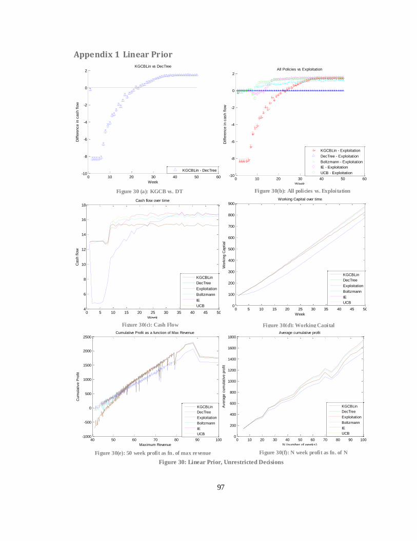
97
Appendix 1 Linear Prior
Figure 30: Linear Prior, Unrestricted Decisions
0 10 20 30 40 50 60-10
-8
-6
-4
-2
0
2
Week
Diffe
rence in c
ash f
low
KGCBLin vs DecTree
KGCBLin - DecTree
0 10 20 30 40 50 60-10
-8
-6
-4
-2
0
2
Week
Diffe
rence in c
ash f
low
All Policies vs Exploitation
KGCBLin - Exploitation
DecTree - Exploitation
Boltzmann - Exploitation
IE - Exploitation
UCB - Exploitation
0 5 10 15 20 25 30 35 40 45 504
6
8
10
12
14
16
18
Week
Cash f
low
Cash flow over time
KGCBLin
DecTree
Exploitation
Boltzmann
IE
UCB0 5 10 15 20 25 30 35 40 45 50
0
100
200
300
400
500
600
700
800
900
Week
Work
ing C
aptial
Working Capital over time
KGCBLin
DecTree
Exploitation
Boltzmann
IE
UCB
40 50 60 70 80 90 100-1000
-500
0
500
1000
1500
2000
2500
Maximum Revenue
Cum
ula
tive P
rofit
Cumulative Profit as a function of Max Revenue
KGCBLin
DecTree
Exploitation
Boltzmann
IE
UCB
0 10 20 30 40 50 60 70 80 90 1000
200
400
600
800
1000
1200
1400
1600
1800
N (number of weeks)
Avera
ge c
um
ula
tive p
rofit
Average cumulative profit
KGCBLin
DecTree
Exploitation
Boltzmann
IE
UCB
Figure 30 (a): KGCB vs. DT Figure 30(b): All policies vs. Exploitation
Figure 30(f): N week profit as fn. of N Figure 30(e): 50 week profit as fn. of max revenue
Figure 30(d): Working Capital Figure 30(c): Cash Flow

98
Figure 31: Linear Prior, Restricted Decisions
0 10 20 30 40 50 60-10
-8
-6
-4
-2
0
2
4
6
8
Week
Diffe
rence in c
ash f
low
KGCBLin vs DecTree
KGCBLin - DecTree
0 10 20 30 40 50 60-10
-8
-6
-4
-2
0
2
Week
Diffe
rence in c
ash f
low
All Policies vs Exploitation
KGCBLin - Exploitation
DecTree - Exploitation
Boltzmann - Exploitation
IE - Exploitation
UCB - Exploitation
0 5 10 15 20 25 30 35 40 45 504
6
8
10
12
14
16
18
Week
Cash f
low
over
tim
e
Cash flow
KGCBLin
DecTree
Exploitation
Boltzmann
IE
UCB0 5 10 15 20 25 30 35 40 45 50
0
100
200
300
400
500
600
700
800
900
Week
Work
ing C
aptial
Working Capital over time
KGCBLin
DecTree
Exploitation
Boltzmann
IE
UCB
40 50 60 70 80 90 100-1000
-500
0
500
1000
1500
2000
2500
3000
Maximum Revenue
Cum
ula
tive P
rofit
Cumulative Profit as a function of Max Revenue
KGCBLin
DecTree
Exploitation
Boltzmann
IE
UCB
0 10 20 30 40 50 60 70 80 90 1000
200
400
600
800
1000
1200
1400
1600
1800
2000
N (number of weeks)
Avera
ge c
um
ula
tive p
rofit
Average cumulative profit
KGCBLin
DecTree
Exploitation
Boltzmann
IE
UCB
Figure 31(a): KGCB vs. DT Figure 31(b): All policies vs. Exploitation
Figure 31(f): N week profit as fn. of N Figure 31(e): 50 week profit as fn. of max revenue
Figure 31(d): Working Capital Figure 31(c): Cash Flow

99
Appendix 2 Pessimistic Prior
Figure 32: Pessimistic Prior, Unrestricted Decisions
0 10 20 30 40 50 60-25
-20
-15
-10
-5
0
5
Week
Diffe
rence in c
ash f
low
KGCBLin vs DecTree
KGCBLin - DecTree
0 10 20 30 40 50 60-20
-10
0
10
20
30
40
Week
Diffe
rence in c
ash f
low
All Policies vs Exploitation
KGCBLin - Exploitation
DecTree - Exploitation
Boltzmann - Exploitation
IE - Exploitation
UCB - Exploitation
0 5 10 15 20 25 30 35 40 45 50-30
-25
-20
-15
-10
-5
0
5
10
15
Week
Cash f
low
Cash flow over time
KGCBLin
DecTree
Exploitation
Boltzmann
IE
UCB
0 5 10 15 20 25 30 35 40 45 50-200
-100
0
100
200
300
400
500
600
Week
Work
ing C
aptial
Working Capital over time
KGCBLin
DecTree
Exploitation
Boltzmann
IE
UCB
40 50 60 70 80 90 100-1500
-1000
-500
0
500
1000
1500
2000
2500
3000
Maximum Revenue
Cum
ula
tive P
rofit
Cumulative Profit as a function of Max Revenue
KGCBLin
DecTree
Exploitation
Boltzmann
IE
UCB
0 10 20 30 40 50 60 70 80 90 100-400
-200
0
200
400
600
800
1000
1200
1400
N (number of weeks)
Avera
ge c
um
ula
tive p
rofit
Average cumulative profit
KGCBLin
DecTree
Exploitation
Boltzmann
IE
UCB
Figure 32(a): KGCB vs. DT Figure 32(b): All policies vs. Exploitation
Figure 32(f): N week profit as fn. of N Figure 32(e): 50 week profit as fn. of max revenue
Figure 32(d): Working Capital Figure 32(c): Cash Flow

100
Perhaps the most notable aspect of the pessimistic prior result is the “hiccup” in the
KGCB policy near week 20. When KGCB realizes it is already half-way through the simulation
period, it tries a few other prices in hopes of finding a new maximum. This only occurs in the
pessimistic prior scenario, not the optimistic prior scenario. One possible explanation is that
KGCB finds that all the prices measured so far yield much higher revenues than originally
expected, so the algorithm is more willing to try new prices even after 20 measurements. Recall
that KGCB maximizes the amount of learning we can gain from measuring a certain price, so
after measuring many alternatives that greatly improved our belief means, it wants to try the
remaining prices. Although it measures a few poor alternatives, it eventually finds a price that
yields higher revenue than the previous optimum, and then performs on par with DT until the end
of the business. DT does not exhibit the same behavior, because it projects three periods into the
future and does not account for how many weeks are left in the simulation, except when it reaches
the very last iterations.
The extremely volatile pure exploitation behavior is also illustrative of pure
exploitation’s susceptibility to the first random revenue observation with a flat prior far below the
truth. Because the first observation is inevitably higher than expected, pure exploitation
continues to sample alternatives near the first. Depending on how high the observation is, pure
exploitation can have very different behavior for the remainder of the algorithm.
If we did not update parameters, but instead updated correlated alternatives, the
performance of all the algorithms would be much worse. Since the prior is overly pessimistic,
almost any price would yield a much higher observation than expected, encouraging the
entrepreneur to continue measuring the same price over and over again. This is a taste of what
happens in the pure exploitation case, but still not as extreme as it would be with a non-
parametric belief structure.

101
Figure 33: Pessimistic Prior, Restricted Decisions
0 10 20 30 40 50 60-15
-10
-5
0
5
10
15
20
25
30
35
Week
Diffe
rence in c
ash f
low
KGCBLin vs DecTree
KGCBLin - DecTree
0 10 20 30 40 50 60-40
-30
-20
-10
0
10
20
30
Week
Diffe
rence in c
ash f
low
All Policies vs Exploitation
KGCBLin - Exploitation
DecTree - Exploitation
Boltzmann - Exploitation
IE - Exploitation
UCB - Exploitation
0 5 10 15 20 25 30 35 40 45 50-30
-25
-20
-15
-10
-5
0
5
10
15
Week
Cash f
low
over
tim
e
Cash flow
KGCBLin
DecTree
Exploitation
Boltzmann
IE
UCB
0 5 10 15 20 25 30 35 40 45 500
100
200
300
400
500
600
Week
Work
ing C
aptial
Working Capital over time
KGCBLin
DecTree
Exploitation
Boltzmann
IE
UCB
30 40 50 60 70 80 90 100 110-2000
-1000
0
1000
2000
3000
4000
Maximum Revenue
Cum
ula
tive P
rofit
Cumulative Profit as a function of Max Revenue
KGCBLin
DecTree
Exploitation
Boltzmann
IE
UCB
0 10 20 30 40 50 60 70 80 90 1000
200
400
600
800
1000
1200
1400
N (number of weeks)
Avera
ge c
um
ula
tive p
rofit
Average cumulative profit
KGCBLin
DecTree
Exploitation
Boltzmann
IE
UCB
Figure 33(a): KGCB vs. DT Figure 33(b): All policies vs. Exploitation
Figure 33(f): N week profit as fn. of N Figure 33(e): 50 week profit as fn. of max revenue
Figure 33(d): Working Capital Figure 33(c): Cash Flow

102
The observations about the unrestricted algorithms are assuaged by the pricing restriction.
The aberrant KGCB behavior is lessened in this case when KGCB cannot choose such extreme
prices to sample. Similarly, exploitation behavior is also much more stable with restricted prices
because its choices are less variable.