AN OPTIMAL 9-POINT FINITE DIFFERENCE SCHEME … · AN OPTIMAL 9-POINT FINITE DIFFERENCE SCHEME FOR...
22
INTERNATIONAL JOURNAL OF c 2013 Institute for Scientific NUMERICAL ANALYSIS AND MODELING Computing and Information Volume 10, Number 2, Pages 389–410 AN OPTIMAL 9-POINT FINITE DIFFERENCE SCHEME FOR THE HELMHOLTZ EQUATION WITH PML ZHONGYING CHEN † , DONGSHENG CHENG † ,WEI FENG † AND TINGTING WU ‡,† Abstract. In this paper, we analyze the defect of the rotated 9-point finite difference scheme, and present an optimal 9-point finite difference scheme for the Helmholtz equation with perfectly matched layer (PML) in two dimensional domain. For this method, we give an error analysis for the numerical wavenumber’s approximation of the exact wavenumber. Moreover, based on minimizing the numerical dispersion, we propose global and refined choice strategies for choosing optimal parameters of the 9-point finite difference scheme. Numerical experiments are given to illustrate the improvement of the accuracy and the reduction of the numerical dispersion. Key words. Helmholtz equation, PML, 9-point finite difference scheme, numerical dispersion. 1. Introduction The Helmholtz equation (1.1) −Δu − k 2 u = f, governs wave propagations and scattering phenomena arising in many areas, for example, in aeronautics, marine technology, geophysics and optical problems. In practice, wave equation modeling in the frequency domain has many advantages over time domain modeling. For example, for certain geometries, only a few frequen- cy components are required to perform wave equation inversion and tomography. Moreover, each frequency can be computed independently, which favors parallel computing. Multiexperiment seismic data can also be simulated economically once the impedance matrix is factored. In addition, modeling the effects of attenuation is more flexible in the frequency domain than in the time domain, because in the frequency domain we can directly input the attenuation coefficient as a function of frequency. To compute the solution of the above problem, due to finite memory of the com- puter, absorbing boundary conditions are needed to truncate the infinite domain into a finite domain, such as one-way approximation (cf. [6, 7, 10]), PML (cf. [4, 5, 15, 26, 30, 31, 33]), and so on. In this paper, PML is used to truncate the domain and absorb the outgoing waves. The technique of PML was proposed by B´ erenger in 1994 (see, [4]). PML has the astonishing property of generating almost no reflection in theory at the interface between the interior medium (the interested domain) and the artificial absorbing medium. The key idea of the PML technique is to introduce an artificial layer with an attenuation parameter around the interior area. The magnitude of the wave is attenuated in the layer while the phase of the wave is conserved. After adding PML to the interior domain, we can impose boundary conditions, like Dirichlet boundary condition, Robin boundary condition and so on, on the outer boundary. Then we obtain a bounded boundary problem, which is usually inverted but ill-conditioned. We refer the interested readers to the Received by the editors October 13, 2011 and, in revised form, March 3, 2012. 2000 Mathematics Subject Classification. 65N06, 65N22, 35L05. 389
Transcript of AN OPTIMAL 9-POINT FINITE DIFFERENCE SCHEME … · AN OPTIMAL 9-POINT FINITE DIFFERENCE SCHEME FOR...

INTERNATIONAL JOURNAL OF c© 2013 Institute for ScientificNUMERICAL ANALYSIS AND MODELING Computing and InformationVolume 10, Number 2, Pages 389–410
AN OPTIMAL 9-POINT FINITE DIFFERENCE SCHEME
FOR THE HELMHOLTZ EQUATION WITH PML
ZHONGYING CHEN†, DONGSHENG CHENG†,WEI FENG† AND TINGTING WU ‡,†
Abstract. In this paper, we analyze the defect of the rotated 9-point finite difference scheme,and present an optimal 9-point finite difference scheme for the Helmholtz equation with perfectlymatched layer (PML) in two dimensional domain. For this method, we give an error analysisfor the numerical wavenumber’s approximation of the exact wavenumber. Moreover, based onminimizing the numerical dispersion, we propose global and refined choice strategies for choosingoptimal parameters of the 9-point finite difference scheme. Numerical experiments are given to
illustrate the improvement of the accuracy and the reduction of the numerical dispersion.
Key words. Helmholtz equation, PML, 9-point finite difference scheme, numerical dispersion.
1. Introduction
The Helmholtz equation
(1.1) −∆u− k2u = f,
governs wave propagations and scattering phenomena arising in many areas, forexample, in aeronautics, marine technology, geophysics and optical problems. Inpractice, wave equation modeling in the frequency domain has many advantagesover time domain modeling. For example, for certain geometries, only a few frequen-cy components are required to perform wave equation inversion and tomography.Moreover, each frequency can be computed independently, which favors parallelcomputing. Multiexperiment seismic data can also be simulated economically oncethe impedance matrix is factored. In addition, modeling the effects of attenuationis more flexible in the frequency domain than in the time domain, because in thefrequency domain we can directly input the attenuation coefficient as a function offrequency.
To compute the solution of the above problem, due to finite memory of the com-puter, absorbing boundary conditions are needed to truncate the infinite domaininto a finite domain, such as one-way approximation (cf. [6, 7, 10]), PML (cf.[4, 5, 15, 26, 30, 31, 33]), and so on. In this paper, PML is used to truncate thedomain and absorb the outgoing waves. The technique of PML was proposed byBerenger in 1994 (see, [4]). PML has the astonishing property of generating almostno reflection in theory at the interface between the interior medium (the interesteddomain) and the artificial absorbing medium. The key idea of the PML techniqueis to introduce an artificial layer with an attenuation parameter around the interiorarea. The magnitude of the wave is attenuated in the layer while the phase ofthe wave is conserved. After adding PML to the interior domain, we can imposeboundary conditions, like Dirichlet boundary condition, Robin boundary conditionand so on, on the outer boundary. Then we obtain a bounded boundary problem,which is usually inverted but ill-conditioned. We refer the interested readers to the
Received by the editors October 13, 2011 and, in revised form, March 3, 2012.2000 Mathematics Subject Classification. 65N06, 65N22, 35L05.
389

390 Z. CHEN, D. CHENG, W. FENG AND T. WU
paper [30] for the solvability and the uniqueness for the Helmholtz equation withPML.
For many years, finite difference methods (cf. [3, 11, 14, 16, 19, 24, 25, 26,27, 32]) and finite element methods (cf. [1, 2, 8, 12, 17]) have been widely usedto discrete the Helmholtz equation (1.1). As is known to all, the solution of theHelmholtz equation oscillates severely for large wavenumbers, and the quality ofthe numerical results usually deteriorates as the wavenumber k increasing (cf. [1,2, 8, 12, 17]). Hence, there is a growing interest in discretization methods where thecomputational complexity increases only moderately with increasing wavenumber(cf. [1, 12, 13, 19, 25]).
Finite-difference frequency-domain modeling for the generation of synthetic seis-mograms and crosshole tomography has been an active field of research since the1980s (see, [25]). Finite difference methods are easily implemented and its compu-tational complexity is much less than that of finite element methods, although thefinite difference method’s accuracy is usually lower than that of the finite elementmethod. In addition, by optimizing the parameters in the finite difference formu-las, we can easily minimize the numerical dispersion (see, [19, 25]). For accuratemodeling, the conventional 5-point finite difference scheme requires 10 gridpointsper wavelength. Therefore, for the Helmholtz equation with large wavenumber-s, the resulting matrix is very large and ill-conditioned. Usually, direct methodsdo not perform well, and iterative methods with preconditioners are alterative (cf.[9, 11, 32]). In 1996, Jo, Shin and Suh proposed the rotated 9-point finite dif-ference scheme for the Helmholtz equation (see, [19]). The approach consists oflinearly combining the two discretizations of the second derivative operator on theclassical Cartesian coordinate system and the 45o rotated system. They also gavea group of optimal parameters based on the normalized phase velocity. This op-timal 9-point scheme reduces the number of gridpoints per wavelength to 5 whilepreserving the accuracy of the conventional 5-point scheme with 10 gridpoints perwavelength. Therefore, computer memory and CPU time are saved. In 1998, Shinand Sohn extended the idea of the rotated 9-point scheme to the 25-point formula,and they obtained a group of optimal parameters by the singular-value decomposi-tion method (see, [25]). Furthermore, the 25-point formula reduces the number ofgridpoints per wavelength to 2. However, the resulting matrix’s bandwidth is muchwider than that of the 9-point scheme, and there are some difficulties when consid-ering the absorbing conditions. To reduce the numerical error, higher-order finitedifference schemes (cf. [3, 26]) were also constructed and widely used. However,to obtain higher-order accuracy, the higher-order schemes require the source termto be smooth enough. Many the practical problems (cf. [22, 23]) are not the case.On the other hand, though that the rotated difference scheme is a popular solverfor the Helmholtz equation, it is not a good choice for the Helmholtz equation withPML. We shall illustrate this in detail in this paper.
This paper is organized as follows. In Section 2, we investigate the rotated 9-point finite difference scheme and show that it is not pointwise consistent with theHelmholtz equation with PML. In Section 3, we present a 9-point difference schemeby using the approach suggested in [26], and prove that it is consistent with theHelmholtz equation with PML and is a second order scheme. For this 9-point differ-ence scheme, we then analyze the error between the numerical wavenumber and theexact wavenumber, and propose global and refined choice strategies for choosingoptimal parameters of the scheme based on minimizing the numerical dispersion.In Section 4, numerical experiments are given to demonstrate the efficiency of the
AN OPTIMAL 9-POINT FD FOR THE HELMHOLTZ EQUATION WITH PML 391
scheme. We show that the scheme proposed in Section 3 improves the accuracyand reduces the numerical dispersion significantly. Finally, Section 5 contains theconclusions of this paper.
2. The Rotated 9-point Finite Difference Scheme for the Helmholtz E-
quation with PML
In this section, we investigate the rotated 9-point finite difference scheme for theHelmholtz equation with PML.
We start with describing the Helmholtz equation with PML [26, 31]. Considerthe Helmholtz equation
∆u+ k2u = 0, in R2,
where ∆ := ∂2/∂x2 + ∂2/∂y2 is the Laplacian, k is the wavenumber defined ask := 2πf/v in which f and v represent the frequency and the velocity respectively,and u is the unknown indicating the pressure of the wave field.
Applying PML technique to truncate the infinite domain into a bounded rect-angular domain leads to the equation
∂
∂x
(
eyex
∂u
∂x
)
+∂
∂y
(
exey
∂u
∂y
)
+ exeyk2u = 0,
where ex := 1 − iσx
ω, ey := 1 − i
σy
ω, in which ω := 2πf denotes the angular fre-
quency, σx and σy are usually chosen as a differentiable function only depending onthe variable x and y respectively for the end of reducing the numerical reflection.Specially,
σx :=
2πa0f0
(
lxLPML
)2
, inside PML,
0, outside PML,
where f0 is the dominant frequency of the source, LPML is the thickness of PML,and lx is the distance from the point (x, y) inside PML and the interface betweenthe interior region and PML region. Moreover, a0 is a constant, and we choosea0 = 1.79 according to the paper [33]. σy can be chosen similarly. Denote
A :=eyex
, B :=exey
, and C := exey,
then we have
(2.1)∂
∂x
(
A∂u
∂x
)
+∂
∂y
(
B∂u
∂y
)
+ Ck2u = 0.
Equation (2.1) can be seen as a general form of the Helmholtz equation (1.1) withits corresponding PML, since in the interior domain, ex ≡ 1 and ey ≡ 1 lead toA = B = C = 1. We call it the Helmholtz-PML equation. Here, we note thatEquation (2.1) is also valid for variable k(x, y) (see, [20, 21]).
We next study the rotated 9-point finite difference scheme (see, [19]). Weconsider the network of grid points (xm, yn), where xm := x0 + (m − 1)h andyn := y0 + (n− 1)h. Notice that the same step size h := ∆x = ∆y is used for bothvariables x and y. Let um,n := u |x=xm,y=yn
represent the pressure of the wavefield at the location (xm, yn), and similarly let km,n := k |x=xm,y=yn
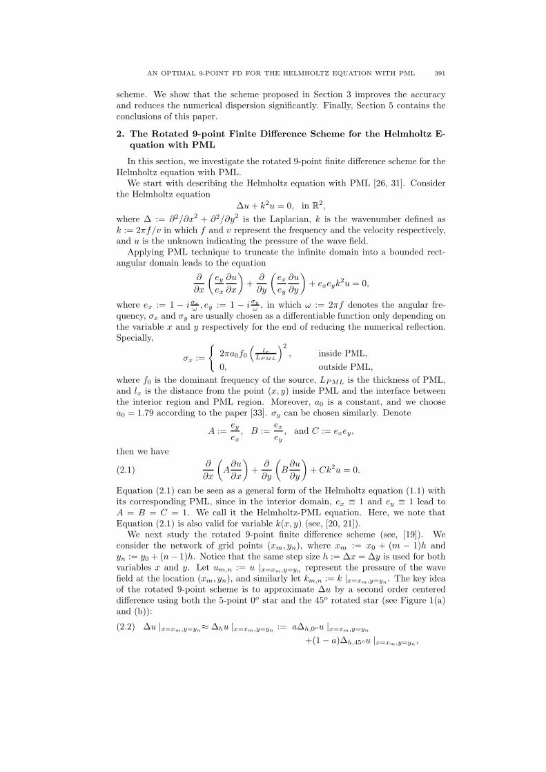
. The key ideaof the rotated 9-point scheme is to approximate ∆u by a second order centereddifference using both the 5-point 0o star and the 45o rotated star (see Figure 1(a)and (b)):
∆u |x=xm,y=yn≈ ∆hu |x=xm,y=yn
:= a∆h,0ou |x=xm,y=yn(2.2)
+(1− a)∆h,45ou |x=xm,y=yn,
392 Z. CHEN, D. CHENG, W. FENG AND T. WU
where
∆h,0ou |x=xm,y=yn:=
1
h2um−1,n + um+1,n + um,n−1 + um,n+1 − 4um,n ,
∆h,45ou |x=xm,y=yn:=
1
2h2um−1,n+1+um+1,n−1+um−1,n−1+um+1,n+1−4um,n,
and a ∈ (0, 1] is a parameter.
x
yy,
x,
45o
(a) (b)
Figure 1. (a) Conventional 0o five-point star, (b) 45o rotated star.
In order to approximate the term of zero order with 9 points, we let
Ih,0o(
k2u)
|x=xm,y=yn:=
1
4
(
k2m−1,num−1,n + k2m+1,num+1,n
+k2m,n−1um,n−1 + k2m,n+1um,n+1
)
,
Ih,45o(
k2u)
|x=xm,y=yn:=
1
4
(
k2m−1,n+1um−1,n+1 + k2m+1,n−1um+1,n−1
+k2m−1,n−1um−1,n−1 + k2m+1,n+1um+1,n+1
)
,
and approximate k2u |x=xm,y=ynby a weighted average:
k2u |x=xm,y=yn≈ Ih
(
k2u)
|x=xm,y=yn,
where
Ih(
k2u)
|x=xm,y=yn:= ck2m,num,n + dIh,0o
(
k2u)
|x=xm,y=yn(2.3)
+eIh,45o(
k2u)
|x=xm,y=yn,
in which c, d, e are parameters satisfying c+ d+ e = 1.These yield the rotated 9-point difference approximation for the Helmholtz e-
quation as
(2.4) ∆hu |x=xm,y=yn+Ih
(
k2u)
|x=xm,y=yn= 0.
Substituting (2.2) and (2.3) into equation (2.4) and replacing um+i,n+j withUm+i,n+j (i, j ∈ Z2 := −1, 0, 1) give the rotated 9-point finite difference equation
(2.5)R1Um−1,n−1 + R2Um,n−1 + R3Um+1,n−1
+ R4Um−1,n + R5Um,n + R6Um+1,n
+ R7Um−1,n+1 + R8Um,n+1 + R9Um+1,n+1 = 0,

AN OPTIMAL 9-POINT FD FOR THE HELMHOLTZ EQUATION WITH PML 393
where the parameters are given by
R1 := 1−a2h2 + e
4k2m−1,n−1, R2 := a
h2 + d4k
2m,n−1, R3 := 1−a
2h2 + e4k
2m+1,n−1,
R4 := ah2 + d
4k2m−1,n, R5 := − 2(1+a)
h2 + ck2m,n, R6 := ah2 + d
4k2m+1,n,
R7 := 1−a2h2 + e
4k2m−1,n+1, R8 := a
h2 + d4k
2m,n+1, R9 := 1−a
2h2 + e4k
2m+1,n+1.
Note that Um,n is intended to approximate um,n, and the parameters a, c, d, eshould be chosen. It is clear that equation (2.5) is a second order difference schemeof the Helmholtz equation (1.1) for arbitrary constants a, c, d and e, if a ∈ (0, 1]and c, d, e satisfy the condition c+ d+ e = 1. The parameters can be optimized forsome purposes. Jo, Shin and Suh [19] provided a group of optimal parameters:
(2.6) a = 0.5461, d = 0.3752, e = −4.0000× 10⁻⁵.
The rotated 9-point finite difference equation (2.5) with parameters (2.6) is a goodscheme for the Helmholtz equation, its numerical dispersion is very small than thatof the conventional 5-point scheme (see, [19]).
To develop the rotated 9-point difference scheme for solving the Helmholtz-PMLequation (2.1), we let
Am+ i2,n+ j
2
:= A(x0 + (m− 1 + i2 )∆x, y0 + (n− 1 + j
2 )∆y),
Bm+ i2,n+ j
2
:= B(x0 + (m− 1 + i2 )∆x, y0 + (n− 1 + j
2 )∆y),
Cm,n := C(x0 + (m− 1)∆x, y0 + (n− 1)∆y),
for i, j ∈ Z3 : = −2,−1, 0, 1, 2. According to the construction of the rotated9-point difference method we define
Lhu |x=xm,y=yn:= aLh,0ou |x=xm,y=yn
+(1− a)Lh,45ou |x=xm,y=yn,
where
Lh,0ou |x=xm,y=yn(2.7)
:=1
h
(
Am+ 1
2,n
um+1,n − um,n
h−Am− 1
2,n
um,n − um−1,n
h
)
+(
Bm,n+ 1
2
um,n+1 − um,n
h−Bm,n− 1
2
um,n − um,n−1
h
)
,
Lh,45ou |x=xm,y=yn(2.8)
:=1√2h
(
Am+ 1
2,n− 1
2
um+1,n−1 − um,n√2h
−Am− 1
2,n+ 1
2
um,n − um−1,n+1√2h
)
+(
Bm+ 1
2,n+ 1
2
um+1,n+1 − um,n√2h
−Bm− 1
2,n− 1
2
um,n − um−1,n−1√2h
)
,
and approximate the first two terms of the left hand side of (2.1) as[ ∂
∂x
(
A∂u
∂x
)
+∂
∂y
(
B∂u
∂y
)]
x=xm,y=yn
≈ Lhu |x=xm,y=yn.
Moreover,(
k2Cu)
|x=xm,y=ynis approximated by
Ih(
k2u)
|x=xm,y=yn:= Ih(k2Cu) |x=xm,y=yn
.(2.9)
These yield the rotated 9-point difference approximation for the Helmholtz-PMLequation (2.1) as
(2.10) Lhu |x=xm,y=yn+Ih
(
k2u)
|x=xm,y=yn= 0.
To analyze this difference approximation, we introduce the concept of consistency(see, [28]).
394 Z. CHEN, D. CHENG, W. FENG AND T. WU
Definition 2.1. Suppose that the partial differential equation under considerationis Lu = f and the corresponding finite difference approximation is Lm,nUm,n =Fm,n where Fm,n denotes whatever approximation which has been made of the sourceterm f . Let (xm, yn) := (x0 + (m − 1)∆x, y0 + (n − 1)∆y). The finite differencescheme Lm,nUm,n = Fm,n is pointwise consistent with the partial differential equa-tion Lu = f at (x, y) if for any smooth function φ = φ(x, y),
(2.11) (Lφ − f) |x=xm,y=yn−[Lm,nφ(xm, yn)− Fm,n] → 0
as ∆x,∆y → 0 and (xm, yn) → (x, y).
For the rotated 9-point finite difference approximation (2.10) of the Helmholtz-PML equation (2.1), we have the following proposition.
Proposition 2.2. The rotated 9-point finite difference approximation (2.10) is notpointwise consistent with the Helmholtz-PML equation (2.1).
Proof. Assume that xm ≤ x < xm+1 and yn ≤ y < yn+1. It follows from (2.7),(2.8) and the Taylor theorem that
Lh,0ou |x=xm,y=yn=
∂
∂x
(
A∂u
∂x
)
+∂
∂y
(
B∂u
∂y
)
+ µ1h2 +O(h3),(2.12)
Lh,45ou |x=xm,y=yn=
1
2
( ∂
∂x− ∂
∂y
)(
A( ∂
∂x− ∂
∂y
)
u)
(2.13)
+( ∂
∂x+
∂
∂y
)(
B( ∂
∂x+
∂
∂y
)
u)
+ µ2h2 +O(h3),
where
µ1 :=1
24
∂3
∂x3
(
A∂u
∂x
)
+∂
∂x
(
A∂3u
∂x3
)
+∂3
∂y3
(
B∂u
∂y
)
+∂
∂y
(
B∂3u
∂y3
)
,
µ2 :=1
48
( ∂
∂x− ∂
∂y
)3(
A( ∂
∂x− ∂
∂y
)
u)
+( ∂
∂x− ∂
∂y
)(
A( ∂
∂x− ∂
∂y
)3
u)
+( ∂
∂x+
∂
∂y
)3(
B( ∂
∂x+
∂
∂y
)
u)
+( ∂
∂x+
∂
∂y
)(
B( ∂
∂x+
∂
∂y
)3
u)
.
Similarly we have
(2.14) Ih(
k2u)
= k2Cu+ µ3h2 +O(h4),
where
µ3 :=1
4(d+ 2e)
( ∂2
∂x2(k2Cu) +
∂2
∂y2(k2Cu)
)
.
Combining equations (2.12) − (2.14) yields that the left hand side of the rotated9-point finite difference approximation (2.10) is equivalent to
a[ ∂
∂x
(
A∂u
∂x
)
+∂
∂y
(
B∂u
∂y
)]
+1− a
2
[ ∂
∂x
(
(A+B)∂u
∂x
)
+∂
∂y
(
(A+B)∂u
∂y
)
+∂
∂x
(
(B − A)∂u
∂y
)
+∂
∂y
(
(B −A)∂u
∂x
)]
+ k2Cu+ ζh2 +O(h3),
where ζ := aµ1 + (1− a)µ2 + µ3.In order to verify this proposition, we need to recall the construction of PML
in Section 2. From the PML’s formulation, we know that there exists some areasatisfying ey ≡ 1 and ex 6= 1. Hence, in such area there hold A = 1
ex, B = ex and

AN OPTIMAL 9-POINT FD FOR THE HELMHOLTZ EQUATION WITH PML 395
C = ex. Combining the above analysis for the rotated 9-point finite difference ap-proximation (2.10), we have that in this area the left hand side of the approximation(2.10) is equivalent to
a[ ∂
∂x
( 1
ex
∂u
∂x
)
+∂
∂y
(
ex∂u
∂y
)]
+1− a
2
[ ∂
∂x
(
(1
ex+ ex)
∂u
∂x
)
+∂
∂y
(
(1
ex+ ex)
∂u
∂y
)
+
(
ex − 1
ex
)
( ∂2u
∂x∂y+
∂2u
∂y∂x
)
+∂
∂x
(
ex − 1
ex
)
∂u
∂y
]
+ k2exu+ ζh2 +O(h3).
As there exist the terms ∂2u∂x∂y
+ ∂2u∂y∂x
and ∂u∂y
, we have the conclusion of this propo-
sition for the area which satisfy both ey ≡ 1 and ex 6= 1. Similar results can beobtained almost everywhere in PML. Therefore, we come to the conclusion of thisproposition.
The above proposition tells us that the rotated 9-point finite difference schemeis not pointwise consistent with the Helmholtz-PML equation. As the convergenceof the finite difference scheme requires that the finite difference scheme should beconsistent with the Helmholtz-PML equation, the rotated 9-point finite differenceapproximation to the Helmholtz-PML equation is not good enough.
3. An Optimal 9-point Finite Difference Scheme for the Helmholtz E-
quation with PML
In this section, we firstly propose a 9-point finite difference scheme which isconsistent with the Helmholtz-PML equation. We then analyze the error betweenthe numerical wavenumber and the exact wavenumber, and present global andrefined optimization rules for choosing the parameters of the finite difference schemesuch that the numerical dispersion is minimized well. Finally we generalize thescheme to the case that different step sizes are used for different variables.
3.1. A Consistent 9-point Difference Scheme. To find a consistent 9-pointdifference scheme for the Helmholtz equation with PML, we follow the approachof constructing finite difference scheme in [26], which was used for the Helmholtzequation with PML in a semi-infinite two-dimensional strip. Here, we note that,compared with the rotated 9-point finite difference scheme, this method is moreeasily extended to the case of different step sizes for different variables, and to thecase of the Helmholtz-PML equation in three dimension domain.
We let
Lh,xu |(m,n+j)(3.1)
:=Am+ 1
2,n+j(um+1,n+j − um,n+j)−Am− 1
2,n+j(um,n+j − um−1,n+j)
h2,
for j ∈ Z2, and define
Lh,xu |x=xm,y=yn:= bLh,xu |(m,n) +
1− b
2
(
Lh,xu |(m,n−1) +Lh,xu |(m,n+1)
)
,
where b ∈ (0, 1] is a constant. Then we approximate the first term of the left handside of (2.1) as
∂
∂x
(
A∂u
∂x
)
|x=xm,y=yn≈ Lh,xu |x=xm,y=yn
.
We deal with the approximation of the second term in a similar way, that is,
∂
∂y
(
B∂u
∂y
)
|x=xm,y=yn≈ Lh,yu |x=xm,y=yn
.

396 Z. CHEN, D. CHENG, W. FENG AND T. WU
Let Lh := Lh,x + Lh,y. We obtain the following 9-point finite difference approx-imation for the Helmholtz-PML equation (2.1)
(3.2) Lhu |x=xm,y=yn+Ih
(
k2u)
|x=xm,y=yn= 0.
The next proposition presents the convergence analysis for the 9-point differencescheme (3.2).
Proposition 3.1. If b ∈ (0, 1] and c+ d+ e = 1, then the 9-point finite differenceapproximation (3.2) is pointwise consistent with the Helmholtz-PML equation (2.1)and is a second order scheme.
Proof. Assume that xm ≤ x < xm+1 and yn ≤ y < yn+1. It follows from the Taylortheorem that
(3.3)[ ∂
∂x
(
A∂u
∂x
)]
|x=xm,y=yn=
∂
∂x
(
A∂u
∂x
)
+ ν1h2 +O(h4),
and
(3.4)[ ∂
∂y
(
B∂u
∂y
)]
|x=xm,y=yn=
∂
∂y
(
B∂u
∂y
)
+ ν2h2 +O(h4),
where
ν1 :=1
24
[ ∂3
∂x3
(
A∂u
∂x
)
+∂
∂x
(
A∂3u
∂x3
)
+ 12(1− b)∂3
∂y2∂x
(
A∂u
∂x
)]
,
ν2 :=1
24
[ ∂3
∂y3
(
B∂u
∂y
)
+∂
∂y
(
B∂3u
∂y3
)
+ 12(1− b)∂3
∂x2∂y
(
B∂u
∂y
)]
.
We recall the Taylor expansion of Ih(
k2u)
, which is given in the equation (2.14),and then revisit the expression of the coefficient µ3 introduced in the middle of theproof of Proposition 2.2. Therefore, together with equations (3.3) and (3.4), wehave that the left hand side of the 9-point finite difference approximation (3.2) isequivalent to
(3.5)∂
∂x
(
A∂u
∂x
)
+∂
∂y
(
B∂u
∂y
)
+ k2Cu+ ηh2 +O(h4),
where η := ν1 + ν2 + µ3. From (3.5) and (2.1) we conclude the results of thisproposition.
From the proposition above, we see that the 9-point finite difference scheme (3.2)is a second order scheme for arbitrary constants b, c, d and e, under the conditionsb ∈ (0, 1] and c+ d+ e = 1. A further observation yields the following proposition.
Proposition 3.2. In the interior area, the rotated 9-point difference scheme (2.4)and the 9-point difference scheme (3.2) are equivalent if a = 2b− 1.
Proof. In the interior area, A = B = C = 1, thus the 9-point difference scheme(3.2) becomes
(3.6)T1Um−1,n−1 + T2Um,n−1 + T3Um+1,n−1
+ T4Um−1,n + T5Um,n + T6Um+1,n
+ T7Um−1,n+1 + T8Um,n+1 + T9Um+1,n+1 = 0,
in which the coefficients are given by
T1 := 1−bh2 + e
4k2m−1,n−1, T2 :=
2b−1h2 + d
4k2m,n−1, T3 := 1−b
h2 + e4k
2m+1,n−1,
T4 := 2b−1h2 + d
4k2m−1,n, T5 := − 4b
h2 + (1 − d− e)k2m,n, T6 := 2b−1h2 + d
4k2m+1,n,
T7 := 1−bh2 + e
4k2m−1,n+1, T8 :=
2b−1h2 + d
4k2m,n+1, T9 := 1−b
h2 + e4k
2m+1,n+1.
AN OPTIMAL 9-POINT FD FOR THE HELMHOLTZ EQUATION WITH PML 397
Comparing the parameters of (2.5) and (3.6) leads to the result of this proposition.
3.2. Choice Strategies for Optimal Parameters of the Finite Difference
Scheme. Since the solution of the Helmholtz equation is oscillating seriously forlarge wavenumbers, to measure the property of a finite difference scheme, only theconvergence order is not enough. In fact, the accuracy of the numerical solutiondeteriorates with increasing wavenumber k. The phenomenon is the so-called ‘pol-lution effect’. As the result of the ‘pollution’, the wavenumber of the numericalsolution is different from the wavenumber of the exact solution, and this is what iscalled ‘numerical dispersion’ (see, [17, 18]). Therefore, to minimize the ‘numericaldispersion’ is to minimize the error between the numerical wavenumber and theexact wavenumber. If the difference scheme has optimal convergence order, andthe parameters are chosen such that the scheme has minimal numerical dispersionin the interior area, then we regard it as an optimal scheme for the Helmholtz-PMLequation (see, [24]).
To optimize the 9-point scheme (3.2), we first perform classical dispersion anal-ysis by assuming a plane-wave solution of the form U(x, y) = e−ik(x cos θ+y sin θ),where θ is the propagation angle from the y-axis. The following analysis is basedon the assumption that the wavenumber k is a positive constant. Moreover, letv be the velocity of propagation, λ be the wavelength, and G be the number ofgridpoints per wavelength, that is, G = λ
h. Since λ = 2πv
ωand k = ω
v, we have
kh = 2πG. Also, denote
P := cos(kh cos θ) = cos(2π
Gcos θ
)
and Q := cos(kh sin θ) = cos(2π
Gsin θ
)
.
We firstly presents the relationship between(
kN)2
and k2, where kN represents
the numerical wavenumber. Substituting Um,n := e−ik(xm cos θ+yn sin θ) into the
equation (3.6), dividing both sides by the factor e−ik(xm cos θ+yn sin θ) and finallyapplying the Euler formula eix = cosx+ i sinx lead to the following equation
2Tc
(
cos(kh sin θ + kh cos θ) + cos(kh sin θ − kh cos θ))
(3.7)
+2Ts
(
cos(kh cos θ) + cos(kh sin θ))
+ To = 0,
where
Tc =1− b
h2+
e
4k2, Ts =
2b− 1
h2+
d
4k2, To = − 4b
h2+ (1 − d− e)k2.
By replacing the variable k in the parameters To, Ts, Tc with kN in equation (3.7),we obtain that
kN =1
h
√
4b+ 2(1− 2b)(P +Q) + 4(b− 1)PQ
(1− d− e) + d2 (P +Q) + ePQ
.(3.8)
The next proposition presents the error between the numerical wavenumber kN andthe exact wavenumber k for the finite difference scheme (3.2).
Proposition 3.3. For the 9-point finite difference scheme (3.2), there holds
kN = k +
[
d
8+
e
4− 1
24+ (
b
8− 5
48) sin2(2θ)
]
k3h2 +O(k4h3), kh → 0.(3.9)
398 Z. CHEN, D. CHENG, W. FENG AND T. WU
Proof. Let τ := kh. Therefore, both P and Q in equation (3.8) depend on τ andθ, that is, P (τ) = cos(τ cos θ), Q(τ) = cos(τ sin θ). In addition, denote
f1(τ) = 4b+ 2(1− 2b) [P (τ) +Q(τ)] + 4(b− 1)P (τ)Q(τ),
f2(τ) = (1− d− e) +d
2[P (τ) +Q(τ)] + eP (τ)Q(τ).
Applying Taylor expansions for f1(τ) and1
f2(τ)at the point τ = 0, we have
f1(τ) = τ2 +1
12
2(b− 1) + (1− 2b)[
(cos θ)4 + (sin θ)4]
(3.10)
+8(b− 1)(cos θ sin θ)2
τ4 +O(τ5),
1
f2(τ)= 1 +
(
d
4+
e
2
)
τ2 +O(τ3).(3.11)
In addition, from the equation (3.8), we have
(
kNh)2
=f1(τ)
f2(τ).
Together with equations (3.10) and (3.11), we obtain
(
kN)2
= k2 +
[
d
4+
e
2− 1
12+ (
b
4− 5
24) sin2(2θ)
]
k4h2 +O(k5h3), kh → 0.
Based on the above equation, applying the Taylor expansion of the function√1 + τ
at the point τ = 0 yields the conclusion of this proposition.
The above proposition indicates that kN approximates k in a second order. More-over, the term associated with k3h2 presents the pollution effect, which dependson the wavenumber k, the parameters of the finite difference formula (3.2) and thewave’s propagation angle θ from the y-axis.
We next present the relationship of the numerical wavenumber kN and the exactwavenumber k. Since h = 2π
Gk, we conclude that
(3.12)kN
k=
G
2π
√
4b+ 2(1− 2b)(P +Q) + 4(b− 1)PQ
(1− d− e) + d2 (P +Q) + ePQ
.
Finally, we choose optimal parameters b, d and e by minimizing the numericaldispersion. To do this, we set
(3.13) J(b, d, e;G, θ) :=G
2π
√
4b+ 2(1− 2b)(P +Q) + 4(b− 1)PQ
(1− d− e) + d2 (P +Q) + ePQ
− 1
for (b, d, e) ∈ (0, 1] × R2 and (G, θ) ∈ IG × Iθ, where IG and Iθ are two intervals.
In general, one can choose Iθ := [0, π2 ] and IG := [Gmin, Gmax] = [4, 400] (see,
[25]). We remark that the interval[
0, π2]
can be replaced by[
0, π4]
because of thesymmetry, and Gmin ≥ 2 based on the Nyquist sampling limit (see, [25]).
It follows from (3.12) that minimizing the error between the numerical wavenum-ber kN and the exact wavenumber k is equivalent to minimizing the norm ‖J(b, d, e; ·, ·)‖∞,IG×Iθ ,which can be formulated as the following rule for the choice of parameters b, d ande.
Rule 3.4. (Global choice strategy)

AN OPTIMAL 9-POINT FD FOR THE HELMHOLTZ EQUATION WITH PML 399
Given intervals Iθ := [0, π2 ] and IG := [4, 400], choose (b, d, e) ∈ (0, 1]× R2 such
that
(3.14) (b, d, e) = arg min‖J(b, d, e; ·, ·)‖∞,IG×Iθ : (b, d, e) ∈ (0, 1]× R2,
which means (b, d, e) is a point in (0, 1]×R2 to minimize the norm ‖J(b, d, e; ·, ·)‖∞,IG×Iθ .
We next remark on the dispersion equation (3.12) by using the physical meaningof the phase velocity and the group velocity. We consider 1-D scalar wave equation(see, [29])
utt − v2uxx = 0,
in which v is a positive constant. This equation admits solutions of the form
(3.15) u(x, t) = ei(ωt−kx),
where ω and k satisfy the relation
(3.16) ω2 = v2k2,
which is called the dispersion relation for the differential equation. Now, it isobvious that (3.15) propagates rightward with t at the speed
(3.17) Vph =ω
k,
which is called the phase velocity. Energy associated with wavenumber k movesasymptotically at the group velocity (cf. [29])
(3.18) Vgr =∂ω
∂k.
Therefore, in a homogeneous, isotropic continuum, there is no dispersion for theexact solution. Waves travel at the phase velocity Vph = ω
k= v, and energy
propagates at the group velocity Vgr = ∂ω∂k
= v. Note that k = 2πGh
. If we regard
the numerical phase velocity and group velocity as V Nph := ωN
kand V N
gr := ∂ωN
∂k
respectively, then we have that
(3.19)V Nph
v=
kN
k,
and
V Ngr
v=
∂ωN
∂k
v=
∂(kNv)∂k
v=
∂kN
∂k.
They are the so-called normalized numerical phase velocity and group velocityrespectively (see, [19, 25]). Moreover, by simple computation,
V Ngr
v=
v
V Nph
G
4π
E
[(1− d− e) + d2 (P +Q) + ePQ]2
,
where
E := − [2(1− 2b)R+ 4(b− 1)W ]L+H
(
d
2R+ eW
)
,
L := (1 − d− e) +d
2(P +Q) + ePQ,
H := 4b+ 2(1− 2b)(P +Q) + 4(b− 1)PQ,
R := cos θ sin(2π
Gcos θ) + sin θ sin(
2π
Gsin θ),
W := cos θ sin(2π
Gcos θ) cos(
2π
Gsin θ) + sin θ cos(
2π
Gcos θ) sin(
2π
Gsin θ).

400 Z. CHEN, D. CHENG, W. FENG AND T. WU
According to the above discussion we have the following remark.
Remark 3.5. If we define the numerical angular frequency and the numerical phase
velocity by ωN := kNv and V Nph := ωN
krespectively, then there holds (3.19), which
implies that minimizing the error between the numerical wavenumber kN and theexact wavenumber k is equivalent to minimizing the error between normalized nu-
merical phase velocityV Nph
vand one.
To implement Rule 3.4, we solve (3.14) numerically by using the least-squaresmethod. To do this, we first set J(b, d, e;G, θ) = 0, which yields the equation
G2
4π2
4b+ 2(1− 2b)(P +Q) + 4(b− 1)PQ
(1− d− e) + d2 (P +Q) + ePQ
= 1.
Thus, we have that
2G2(1− P −Q+ PQ)b+ π2(2− P −Q)d+ 2π2(1 − PQ)e(3.20)
= 2π2 +G2(2PQ− P −Q).
Note that P andQ are functions ofG and θ. We choose θ = θm = (m−1)π4(l−1) ∈ Iθ, m =
1, 2, . . . , l, and 1G
= 1Gn
= 1Gmax
+(n− 1)1
Gmin− 1
Gmax
r−1 ∈ [ 1Gmax
, 1Gmin
], n = 1, 2, . . . , r.
Then, equation (3.20) leads to the linear system
(3.21)
S11,1 S2
1,1 S31,1
......
...S11,r S2
1,r S31,r
......
...S1m,n S2
m,n S3m,n
......
...S1l,r S2
l,r S3l,r
bde
=
S41,1...
S41,r...
S4m,n
...S4l,r
,
where
S1m,n := 2G2
n
[
1− cos( 2π
Gn
cos θm
)
− cos( 2π
Gn
sin θm
)
+cos( 2π
Gn
cos θm
)
cos( 2π
Gn
sin θm
)]
,
S2m,n := π2
[
2− cos( 2π
Gn
cos θm
)
− cos( 2π
Gn
sin θm
)
]
,
S3m,n := 2π2
[
1− cos( 2π
Gn
cos θm
)
cos( 2π
Gn
sin θm
)
]
,
S4m,n := 2π2 +G2
n
[
2 cos( 2π
Gn
cos θm
)
cos( 2π
Gn
sin θm
)
− cos( 2π
Gn
cos θm
)
− cos( 2π
Gn
sin θm
)]
.
The coefficient matrix of (3.21) has l× r rows and 3 columns, thus it is an over-determined system. Following the paper [25], by choosing l = 10, r = 100, andusing the least-squares method to solve (3.21), we obtain the optimal parametersfor difference scheme (3.2):
(3.22) b = 0.7926, d = 0.3768, e = −0.0064.
AN OPTIMAL 9-POINT FD FOR THE HELMHOLTZ EQUATION WITH PML 401
We call the difference scheme (3.2) with parameters (3.22) as the global optimal9-point scheme for the Helmholtz-PML equation (or simply the global 9p).
We remark that the above method was used in [25] for choosing optimal pa-rameters of the 25-point finite difference scheme, while the rotated 9-point finitedifference scheme proposed in [19] used the L2-norm of the residual, that is
∫∫
[V Nph
v− 1
]2
dGdθ.
In practical computation, parameters provided in (3.22) seems much better thanthat obtained by using the L2-norm, especially for large wavenumbers.
We observe that optimal parameters obtained by Rule 3.4 are roughly chosen.Only one group of parameters is obtained and used to the computation for differentfrequencies, velocities and step sizes. This may yield much numerical dispersion forlarge wavenumbers and variable k(x, y) (see examples in Section 4). To reduce thenumerical dispersion and improve the accuracy of the difference scheme, we proposethe following rule.
Rule 3.6. (Refined choice strategy)Step 1. Estimate the interval IG := [Gmin, Gmax].Step 2. Choose (b, d, e) ∈ (0, 1]× R
2 such that
(3.23) (b, d, e) = arg min‖J(b, d, e; ·, ·)‖∞,IG×Iθ : (b, d, e) ∈ (0, 1]× R2.
In general, we can estimate IG by using a priori information before choosingparameters. For example, if the frequency f ∈ [fmin, fmax] and the velocity v ∈[vmin, vmax] then for a given step size h we have Gmin := vmin
hfmax
and Gmax := vmax
hfmin
.
As a result, we shall obtain a group of appropriate parameters for the differencescheme, which is much better than that obtained from the global choice strategyRule 3.4.
In the following table, we present some groups of refined optimal parameters.
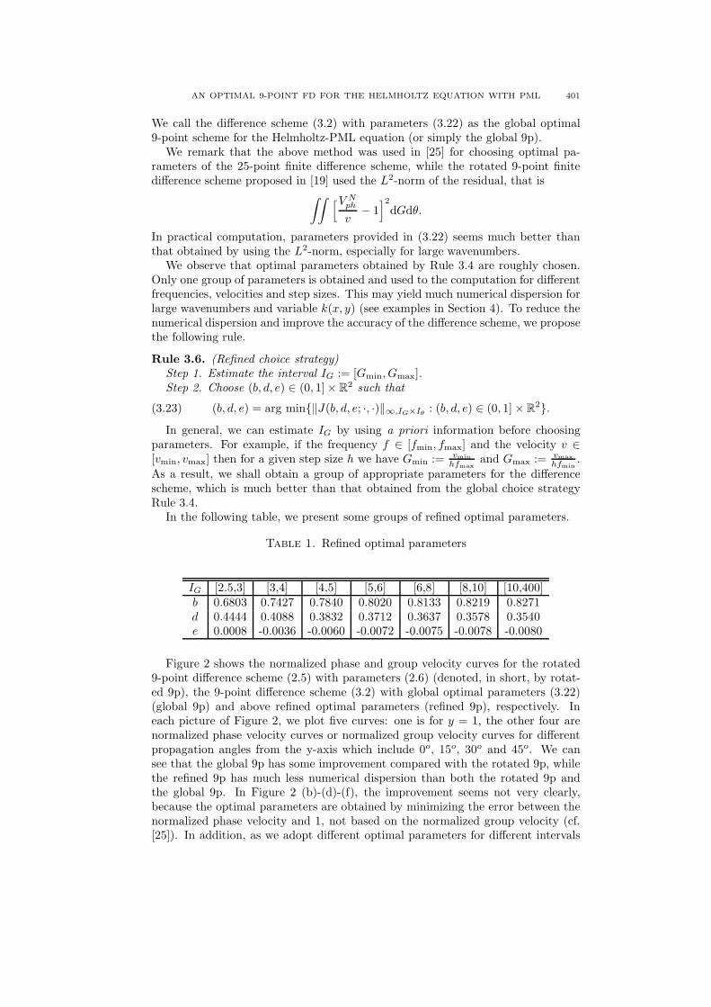
Table 1. Refined optimal parameters
IG [2.5,3] [3,4] [4,5] [5,6] [6,8] [8,10] [10,400]b 0.6803 0.7427 0.7840 0.8020 0.8133 0.8219 0.8271d 0.4444 0.4088 0.3832 0.3712 0.3637 0.3578 0.3540e 0.0008 -0.0036 -0.0060 -0.0072 -0.0075 -0.0078 -0.0080
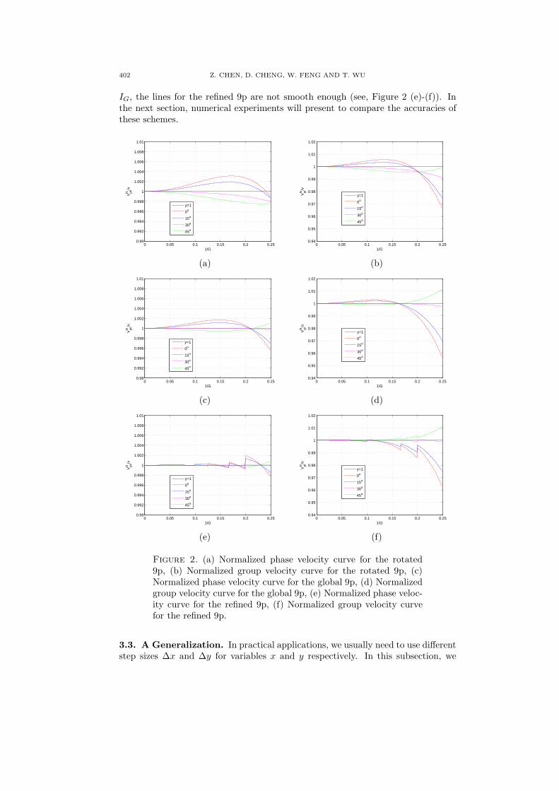
Figure 2 shows the normalized phase and group velocity curves for the rotated9-point difference scheme (2.5) with parameters (2.6) (denoted, in short, by rotat-ed 9p), the 9-point difference scheme (3.2) with global optimal parameters (3.22)(global 9p) and above refined optimal parameters (refined 9p), respectively. Ineach picture of Figure 2, we plot five curves: one is for y = 1, the other four arenormalized phase velocity curves or normalized group velocity curves for differentpropagation angles from the y-axis which include 0o, 15o, 30o and 45o. We cansee that the global 9p has some improvement compared with the rotated 9p, whilethe refined 9p has much less numerical dispersion than both the rotated 9p andthe global 9p. In Figure 2 (b)-(d)-(f), the improvement seems not very clearly,because the optimal parameters are obtained by minimizing the error between thenormalized phase velocity and 1, not based on the normalized group velocity (cf.[25]). In addition, as we adopt different optimal parameters for different intervals
402 Z. CHEN, D. CHENG, W. FENG AND T. WU
IG, the lines for the refined 9p are not smooth enough (see, Figure 2 (e)-(f)). Inthe next section, numerical experiments will present to compare the accuracies ofthese schemes.
0 0.05 0.1 0.15 0.2 0.250.99
0.992
0.994
0.996
0.998
1
1.002
1.004
1.006
1.008
1.01
1/G
VphN
/v
y=1
0o
15o
30o
45o
0 0.05 0.1 0.15 0.2 0.250.94
0.95
0.96
0.97
0.98
0.99
1
1.01
1.02
1/G
VgrN
/v
y=1
0o
15o
30o
45o
(a) (b)
0 0.05 0.1 0.15 0.2 0.250.99
0.992
0.994
0.996
0.998
1
1.002
1.004
1.006
1.008
1.01
1/G
VphN
/v
y=1
0o
15o
30o
45o
0 0.05 0.1 0.15 0.2 0.250.94
0.95
0.96
0.97
0.98
0.99
1
1.01
1.02
1/G
VgrN
/v
y=1
0o
15o
30o
45o
(c) (d)
0 0.05 0.1 0.15 0.2 0.250.99
0.992
0.994
0.996
0.998
1
1.002
1.004
1.006
1.008
1.01
1/G
VphN
/v
y=1
0o
15o
30o
45o
0 0.05 0.1 0.15 0.2 0.250.94
0.95
0.96
0.97
0.98
0.99
1
1.01
1.02
1/G
VgrN
/v
y=1
0o
15o
30o
45o
(e) (f)
Figure 2. (a) Normalized phase velocity curve for the rotated9p, (b) Normalized group velocity curve for the rotated 9p, (c)Normalized phase velocity curve for the global 9p, (d) Normalizedgroup velocity curve for the global 9p, (e) Normalized phase veloc-ity curve for the refined 9p, (f) Normalized group velocity curvefor the refined 9p.
3.3. A Generalization. In practical applications, we usually need to use differentstep sizes ∆x and ∆y for variables x and y respectively. In this subsection, we
AN OPTIMAL 9-POINT FD FOR THE HELMHOLTZ EQUATION WITH PML 403
generalize the 9-point scheme (3.2) to this case and show how to optimize thecorresponding parameters.
We denote
L∆x,xu |(m,n+j)(3.24)
:=Am+ 1
2,n+j(um+1,n+j − um,n+j)−Am− 1
2,n+j(um,n+j − um−1,n+j)
(∆x)2 ,
for j ∈ Z2, and define
L∆x,xu |x=xm,y=yn:= bL∆x,xu |(m,n) +
1− b
2
(
L∆x,xu |(m,n−1) +L∆x,xu |(m,n+1)
)
,
where b ∈ (0, 1] is a constant. Then the first term of the left hand side of (2.1) isapproximated as
∂
∂x
(
A∂u
∂x
)
|x=xm,y=yn≈ L∆x,xu |x=xm,y=yn
.
The approximation of the second term is dealt with in a similar way, that is,
∂
∂y
(
B∂u
∂y
)
|x=xm,y=yn≈ L∆y,yu |x=xm,y=yn
.
Let L∆x,∆y := L∆x,x + L∆y,y. We obtain the following 9-point finite differenceapproximation for the Helmholtz-PML equation (2.1)
(3.25) L∆x,∆yu |x=xm,y=yn+Ih
(
k2u)
|x=xm,y=yn= 0.
Remark 3.7. If c + d + e = 1, then the 9-point finite difference approximation(3.25) is consistent with Helmholtz-PML equation (2.1).
When ∆x = h, ∆y = γh (γ is a positive constant), performing classical disper-sion analysis to the finite difference method (3.25) yields
(3.26) kN =1
h
√
W
L,
where
W := 2b(
1 + 1γ2
)
+ 2[
1− b(
1 + 1γ2
)]
P + 2(
1−bγ2 − b
)
Q+ 2(b− 1)(
1 + 1γ2
)
P Q,
L := (1− d− e) + d2
(
P + Q)
+ eP Q,
in which
P := cos (γkh cos θ) = cos
(
γ2π
Gcos θ
)
, Q := cos (kh sin θ) = cos
(
2π
Gsin θ
)
.
As h = 2πGk
, we conclude that
(3.27)kN
k=
G
2π
√
W
L.
Similarly as before, we choose optimal parameters b, d and e by minimizing thenumerical dispersion. To do this, we define the functional
(3.28) Jγ(b, d, e;G, θ) :=G
2π
√
W
L− 1.
It follows from (3.27) that minimizing the error between the numerical wavenum-ber kN and the exact wavenumber k is equivalent to minimizing the norm ‖Jγ(b, d, e; ·, ·)‖∞,IG,Iθ .
404 Z. CHEN, D. CHENG, W. FENG AND T. WU
The corresponding refined choice strategy can be obtained by replacing ‖J(b, d, e; ·, ·)‖∞,IG×Iθ
in Rule 3.6 with ‖Jγ(b, d, e; ·, ·)‖∞,IG×Iθ .
Rule 3.8. (Refined choice strategy II)Step 1. Estimate the interval IG := [Gmin, Gmax].Step 2. Choose (b, d, e) ∈ (0, 1]× R
2 such that
(3.29) (b, d, e) = arg min‖Jγ(b, d, e; ·, ·)‖∞,IG×Iθ : (b, d, e) ∈ (0, 1]× R2.
To implement Rule 3.8, we set Jγ(b, d, e;G, θ) = 0 to obtain the equation
G2
(
1 +1
γ2
)
(
1− P − Q+ P Q)
b + π2(
2− P − Q)
d+ 2π2(
1− P Q)
e(3.30)
= 2π2 +G2
[(
1 +1
γ2
)
P Q − P − 1
γ2Q
]
.
Dealing with the equation (3.30) as we did with the equation (3.20) yields therefined optimal parameters for the finite difference scheme (3.25).
For the convenience of analysis, we also present the normalized numerical phasevelocity and group velocity here. The normalized numerical phase velocity is
(3.31)V Nph
v=
kN
k,
and the normalized numerical group velocity is
(3.32)V Ngr
v=
v
V Nph
G
4π
K
L2,
where
K := HL− W
[
e(
EQ+ P F)
+d
2
(
E + F)
]
,
in which
H := 2(b− 1)(
1 + 1γ2
)(
EQ + P F)
+ 2[
1− b(
1 + 1γ2
)]
E + 2(
1−bγ2 − b
)
F ,
E := −γ cos θ sin(
γ 2πG
cos θ)
, F := − sin θ sin(
2πG
sin θ)
.
4. Numerical Experiments
In this section, we present two numerical experiments to illustrate the efficiencyof the schemes described in the last section. All the experiments are performedwith Matlab 7v on an Intel Xeon (8-core) with 3.33GHz and 96Gb RAM.
4.1. An Numerical Example for the Helmholtz Equation. Consider theHelmholtz equation
(4.1) −∆u− k2u = 0, in Ω : = (0, 1)× (0, 1),
with boundary conditions
(4.2) iku+∂u
∂n= g, on Γ : = ∂Ω.
The function g depends on the parameter θ and is given by
g(x) =
i(k − k2)eik1x1 , if x ∈ Γ1 : = (0, 1)× (0, 0),
i(k + k1)ei(k1+k2x2), if x ∈ Γ2 : = (1, 1)× (0, 1),
i(k + k2)ei(k1x1+k2), if x ∈ Γ3 : = (1, 0)× (1, 1),
i(k − k1)eik2x2 , if x ∈ Γ4 : = (0, 0)× (1, 0),

AN OPTIMAL 9-POINT FD FOR THE HELMHOLTZ EQUATION WITH PML 405
with (k1, k2) = k(cos θ, sin θ). The exact solution of this problem is
u(x) : = ei(k1x1+k2x2).
This problem was used for measuring the efficiency of numerical methods in [1].We use it to measure the accuracy for four different schemes, including the con-ventional 5-point scheme (5p), the rotated 9p, the global 9p and the refined 9p.The error is measured in C-norm, which is defined as: for any complex vectorz = [z1, z2, . . . , zM ],
‖z‖C := max1≤j≤M
|zj|,
where |zj | is the complex modulus of zj . The parameters in Table 1 are used asrefined optimal parameters.
Tables 2, 3 and 4 show the error in the C-norm for different schemes with differentgridpointsN per line for the case θ = π
4 with k = 30, 200 and 500 respectively. Fromthese tables we see that there are significant improvements of the accuracy one byone, and all of the four schemes are second order formulas. Among three 9-pointschemes, the refined 9p improves the accuracy most prominently, especially forlarge wavenumbers. The refined 9p only needs half of the number of gridpointsto obtain the same accuracy of the rotated 9p. Specifically, from Table 3 we seethat when k = 200, the accuracy of the refined 9p for N = 129 is comparableto that of the rotated 9p for N = 257, which means that the accuracy of therefined 9p with 4 gridpoints per wavelength is comparable with that of the rotated9p with 8 gridpoints per wavelength. In addition, from Table 4 we also find thatwhen k = 500, the accuracy of the refined 9p with 6 gridpoints per wavelength iscomparable with that of the rotated 9p with 13 gridpoints per wavelength.
Table 2. The error in the C-norm for k = 30
N 33 65 129 257 5135p 0.9743 0.2325 0.0569 0.0142 0.0035
rotated 9p 0.1537 0.0391 0.0098 0.0025 0.0006global 9p 0.1274 0.0330 0.0083 0.0021 0.0005refined 9p 0.1186 0.0291 0.0073 0.0018 4.5131e-04
Table 3. The error in the C-norm for k = 200
N 129 257 513 10255p 3.7186 2.9475 1.1732 0.2964
rotated 9p 1.0258 0.4747 0.1298 0.0331global 9p 0.5679 0.2154 0.0698 0.0186refined 9p 0.4845 0.0861 0.0216 0.0057
Figure 3 gives an intuitive comparison between the rotated 9p, the global 9p andthe refined 9p. It is easy to see that for large wavenumber k, the improvement ofthe refined 9p over other two schemes is very obvious.
Further comparison among the rotated 9p, the global 9p and the refined 9p isgiven in Figure 4. Figure 4 (a) presents the error in C-norm of three schemes forthe case kh = 1, and Figure 4 (b) shows the case kh = 0.5. The wavenumber k in
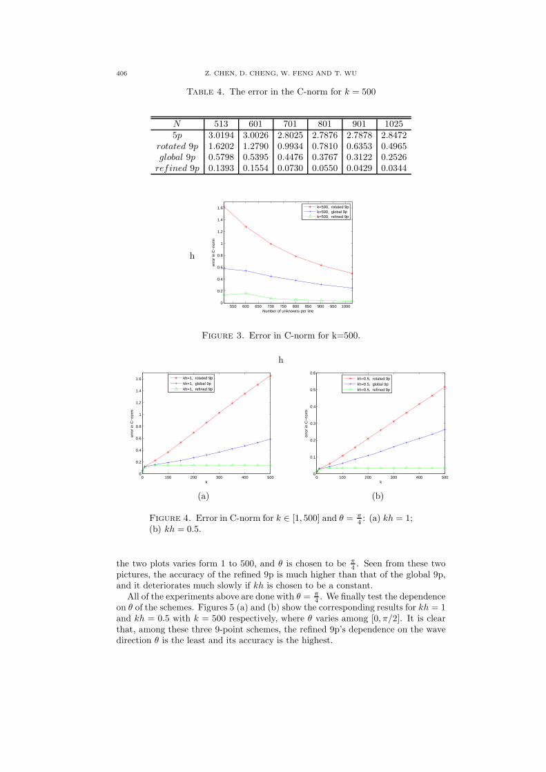
406 Z. CHEN, D. CHENG, W. FENG AND T. WU
Table 4. The error in the C-norm for k = 500
N 513 601 701 801 901 10255p 3.0194 3.0026 2.8025 2.7876 2.7878 2.8472
rotated 9p 1.6202 1.2790 0.9934 0.7810 0.6353 0.4965global 9p 0.5798 0.5395 0.4476 0.3767 0.3122 0.2526refined 9p 0.1393 0.1554 0.0730 0.0550 0.0429 0.0344
h
550 600 650 700 750 800 850 900 950 10000
0.2
0.4
0.6
0.8
1
1.2
1.4
1.6er
ror
in C
−no
rm
Number of unknowns per line
k=500, rotated 9pk=500, global 9pk=500, refined 9p
Figure 3. Error in C-norm for k=500.
h
0 100 200 300 400 5000
0.2
0.4
0.6
0.8
1
1.2
1.4
1.6
k
erro
r in
C−
norm
kh=1, rotated 9pkh=1, global 9pkh=1, refined 9p
0 100 200 300 400 5000
0.1
0.2
0.3
0.4
0.5
0.6
k
erro
r in
C−
norm
kh=0.5, rotated 9pkh=0.5, global 9pkh=0.5, refined 9p
(a) (b)
Figure 4. Error in C-norm for k ∈ [1, 500] and θ = π4 : (a) kh = 1;
(b) kh = 0.5.
the two plots varies form 1 to 500, and θ is chosen to be π4 . Seen from these two
pictures, the accuracy of the refined 9p is much higher than that of the global 9p,and it deteriorates much slowly if kh is chosen to be a constant.
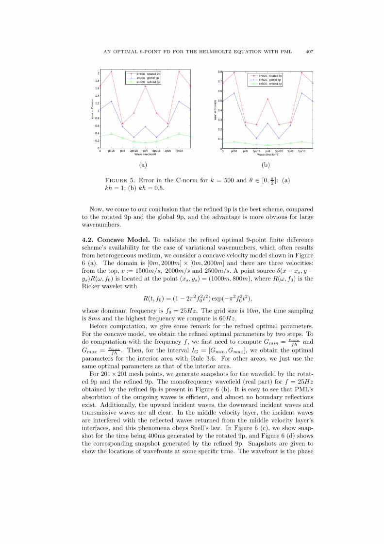
All of the experiments above are done with θ = π4 . We finally test the dependence
on θ of the schemes. Figures 5 (a) and (b) show the corresponding results for kh = 1and kh = 0.5 with k = 500 respectively, where θ varies among [0, π/2]. It is clearthat, among these three 9-point schemes, the refined 9p’s dependence on the wavedirection θ is the least and its accuracy is the highest.
AN OPTIMAL 9-POINT FD FOR THE HELMHOLTZ EQUATION WITH PML 407
0 pi/16 pi/8 3pi/16 pi/4 5pi/16 3pi/8 7pi/160
0.2
0.4
0.6
0.8
1
1.2
1.4
1.6
1.8
2
Wave direction θ
erro
r in
C−
norm
k=500, rotated 9pk=500, global 9pk=500, refined 9p
0 pi/16 pi/8 3pi/16 pi/4 5pi/16 3pi/8 7pi/160
0.1
0.2
0.3
0.4
0.5
0.6
0.7
0.8
Wave direction θ
erro
r in
C−
norm
k=500, rotated 9pk=500, global 9pk=500, refined 9p
(a) (b)
Figure 5. Error in the C-norm for k = 500 and θ ∈ [0, π2 ]: (a)kh = 1; (b) kh = 0.5.
Now, we come to our conclusion that the refined 9p is the best scheme, comparedto the rotated 9p and the global 9p, and the advantage is more obvious for largewavenumbers.
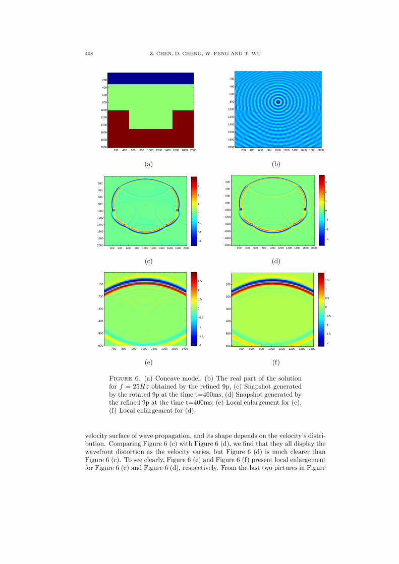
4.2. Concave Model. To validate the refined optimal 9-point finite differencescheme’s availability for the case of variational wavenumbers, which often resultsfrom heterogeneous medium, we consider a concave velocity model shown in Figure6 (a). The domain is [0m, 2000m] × [0m, 2000m] and there are three velocities:from the top, v := 1500m/s, 2000m/s and 2500m/s. A point source δ(x − xs, y −ys)R(ω, f0) is located at the point (xs, ys) = (1000m, 800m), where R(ω, f0) is theRicker wavelet with
R(t, f0) = (1 − 2π2f20 t
2) exp(−π2f20 t
2),
whose dominant frequency is f0 = 25Hz. The grid size is 10m, the time samplingis 8ms and the highest frequency we compute is 60Hz.
Before computation, we give some remark for the refined optimal parameters.For the concave model, we obtain the refined optimal parameters by two steps. Todo computation with the frequency f , we first need to compute Gmin = vmin
fhand
Gmax = vmax
fh. Then, for the interval IG = [Gmin, Gmax], we obtain the optimal
parameters for the interior area with Rule 3.6. For other areas, we just use thesame optimal parameters as that of the interior area.
For 201× 201 mesh points, we generate snapshots for the wavefield by the rotat-ed 9p and the refined 9p. The monofrequency wavefield (real part) for f = 25Hzobtained by the refined 9p is present in Figure 6 (b). It is easy to see that PML’sabsorbtion of the outgoing waves is efficient, and almost no boundary reflectionsexist. Additionally, the upward incident waves, the downward incident waves andtransmissive waves are all clear. In the middle velocity layer, the incident wavesare interfered with the reflected waves returned from the middle velocity layer’sinterfaces, and this phenomena obeys Snell’s law. In Figure 6 (c), we show snap-shot for the time being 400ms generated by the rotated 9p, and Figure 6 (d) showsthe corresponding snapshot generated by the refined 9p. Snapshots are given toshow the locations of wavefronts at some specific time. The wavefront is the phase
408 Z. CHEN, D. CHENG, W. FENG AND T. WU
200 400 600 800 1000 1200 1400 1600 1800 2000
200
400
600
800
1000
1200
1400
1600
1800
2000200 400 600 800 1000 1200 1400 1600 1800 2000
200
400
600
800
1000
1200
1400
1600
1800
2000
(a) (b)
200 400 600 800 1000 1200 1400 1600 1800 2000
200
400
600
800
1000
1200
1400
1600
1800
2000
−3
−2
−1
0
1
2
3
200 400 600 800 1000 1200 1400 1600 1800 2000
200
400
600
800
1000
1200
1400
1600
1800
2000
−3
−2
−1
0
1
2
3
(c) (d)
700 800 900 1000 1100 1200 1300 1400
100
200
300
400
500
600 −2
−1.5
−1
−0.5
0
0.5
1
1.5
700 800 900 1000 1100 1200 1300 1400
100
200
300
400
500
600−2
−1.5
−1
−0.5
0
0.5
1
1.5
(e) (f)
Figure 6. (a) Concave model, (b) The real part of the solutionfor f = 25Hz obtained by the refined 9p, (c) Snapshot generatedby the rotated 9p at the time t=400ms, (d) Snapshot generated bythe refined 9p at the time t=400ms, (e) Local enlargement for (c),(f) Local enlargement for (d).
velocity surface of wave propagation, and its shape depends on the velocity’s distri-bution. Comparing Figure 6 (c) with Figure 6 (d), we find that they all display thewavefront distortion as the velocity varies, but Figure 6 (d) is much clearer thanFigure 6 (c). To see clearly, Figure 6 (e) and Figure 6 (f) present local enlargementfor Figure 6 (c) and Figure 6 (d), respectively. From the last two pictures in Figure
AN OPTIMAL 9-POINT FD FOR THE HELMHOLTZ EQUATION WITH PML 409
6, some unphysical oscillations in the background, such as in depth 200m, can befound in the former, but these do not exist in the latter. Therefore, the efficiencyof the refined 9p is confirmed.
5. Conclusions
We summarize and comment on the numerical results. We had proved thatthe rotated 9-point finite difference scheme is not pointwise consistent with theHelmholtz-PML equation, though it is a popular scheme for the Helmholtz equation.Then, we presented a consistent 9-point difference scheme for the Helmholtz-PMLequation. For this method, we gave an error analysis for the numerical wavenum-ber’s approximation of the exact wavenumber, and proposed global and refinedchoice strategies for choosing optimal parameters based on minimizing the numer-ical dispersion. Finally, numerical experiments were presented to confirm that therefined 9p is a good choice for the Helmholtz-PML equation, compared with therotated 9p and the global 9p, as the refined 9p possesses the highest accuracy andthe smallest numerical dispersion, especially for large wavenumbers.
Acknowledgments
This research is partially supported by the Natural Science Foundation of Chi-na under grants 10771224 and 11071264, the Science and Technology Section ofSINOPEC and Guangdong Provincial Government of China through the “Compu-tational Science Innovative Research Team” program.
References
[1] I. Babuska, F. Ihlenburg, E. T. Paik and S. A. Sauter, A genralized finite element method forsolving the Helmholtz equation in two dimensions with minimal pollution, Computer Methods
in Applied Mechanics and Engineering, 128 (1995), 325-359.[2] I. Babuska and S. A. Sauter, Is the pollution effect of the FEM avoidable for the Helmholtz
equation considering high wave numbers? SIAM Review, 42 (2000), 451-484.[3] G. Baruch, G. Fibich, S. Tsynkov and E. Turkel, Fourth order schemes for time-harmonic
wave equations with discontinuous coefficients, Communications in Computational Physics,
5 (2009), 442-455.[4] J.-P. Berenger, A perfectly matched layer for the absorption of electromagnetic waves, Journal
of Computational Physics, 114 (1994), 185-200.[5] W. C. Chew, J. M. Jin and E. Michielssen, Complex coordinate stretching as a generalized
absorbing boundary condition, Microwave and Optical Technology Letters, 15 (1997), 363-369.
[6] R. Clayton and B. Engquist, Absorbing boundary conditions for acoustic and elastic waveequations, Bulletin of the Seismological Society of American, 67 (1977), 1529-1540.
[7] R. W. Clayton and B. Engquist, Absorbing boundary conditions for wave-equations migra-tion, Geophysics, 45 (1980), 895-904.
[8] A. Deraemaeker, I. Babuska and P. Bouillard, Dispersion and pollution of the FEM sollutionfor the Helmholtz equation in one, two and three dimensions, International Journal for
Numerical Methods in Engineering, 46 (1999), 471-499.[9] P. M. De Zeeuw, Matrix-dependent prolongations and restrictions in a blackbox multigrid
solver, Journal of Computational and Applied Mathematics, 33 (1990), 1-27.[10] B. Engquist and A. Majda, Absorbing boundary conditions for the numerical simulation of
waves, Mathematics of Computation, 31 (1977), 629-651.[11] Y. A. Erlangga, C. W. Oosterlee and C. Vuik, A novel multigrid based preconditioner for
heterogeneous Helmholtz problems, SIAM Journal on Scientific Computing, 27 (2006), 1471-1492.
[12] X. Feng and H. Wu, Discontinuous galerkin methods for the Helmholtz equation with largewave number, SIAM Journal on Numerical Analysis, 47 (2009), 2872-2896.
[13] Y. Guo and F. Ma, Some domain decomposition methods employing the PML techniquefor the Helmholtz equation, Numerical Mathematics A Journal of Chinese Universities, 31(2009), 369-384.
410 Z. CHEN, D. CHENG, W. FENG AND T. WU
[14] I. Harari and E. Turkel, Accurate finite difference methods for time-harmonic wave propaga-tion, Journal of Computational Physics, 119 (1995), 252-270.
[15] F. D. Hastings, J. B. Schneider and S.L. Broschat, Application of the perfectly matchedlayer(PML) absorbing boundary condition to elastic wave propagation, Journal of AcousticalSociety of America, 100 (1996), 3061-3069.
[16] B. Hustedt, S. Operto and J. Virieux, Mixed-grid and staggered-grid finite-difference meth-ods for frequency-domain acoustic wave modelling, Geophysical Journal International, 157(2004), 1269-1296.
[17] F. Ihlenburg and I. Babuska, Finite element solution of the Helmholtz equation with high wavenumber, Part I: The h-version of the FEM, Computers & Mathematics with Applications, 30
(1995), 9-37.[18] F. Ihlenburg and I. Babuska, Dispersion analysis and error estimation of galerkin finite ele-
ment methods for the Helmholtz equation, International Journal for Numerical Methods in
Engineering, 38 (1995), 3745-3774.[19] C.-H. Jo, C. Shin and J. H. Suh, An optimal 9-point, finite-difference, frequency-space, 2-D
scalar wave extrapolator, Geophysics, 61 (1996), 529-537.[20] J. W. Kang and L. F. Kallivokas, Mixed unsplit-field perfectly matched layers for transient
simulations of scalar waves in heterogeneous domains, Computers & Geosciences, 14 (2010),623-648.
[21] J. W. Kang and L. F. Kallivokas, The inverse medium problem in heterogeneous PML-truncated domains using scalar probing waves, Computer Methods in Applied Mechanics and
Engineering, 200 (2011), 265-283.[22] R. G. Pratt, C. Shin and G. J. Hicks, Gauss-Newton and full Newton methods in frequency-
space seismic waveform inversion, Geophysical Journal International, 133 (1998), 341-362.[23] R. G. Pratt and M. H. Worthington, Inverse theory applied to multi-source cross-hole tompg-
raphy. Part 1: Acoustic wave-equation method, Geophysical Prospecting, 38 (1990), 287-310.[24] H. Ren, H. Wang and T. Gong, Seismic modeling of scalar seismic wave propagation with
finite difference scheme in frequency-space domain, Geophysical Prospecting for Petroleum,
48 (2009), 20-27.[25] C. Shin and H. Sohn, A frequency-space 2-D scalar wave exteapolator using extended 25-point
finite-difference operator, Geophysics, 63 (1998), 289-296.[26] I. Singer and E. Turkel, A perfectly matched layer for the Helmholtz equation in a semi-infinite
strip, Journal of Computational Physics, 201 (2004), 439-465.[27] I. Singer and E. Turkel, High-order finite difference methods for the Helmholtz equation,
Computer Methods in Applied Mechanics and Engineering, 163 (1998), 343-358.[28] J. W. Thomas, Numerical Partial Differential Equations, Finite Difference Methods,
Springer, New York, 1995.[29] L. N. Trefethen, Group velocity in finite difference schemes, SIAM Review, 24 (1982), 113-136.[30] S. Tsynkov and E. Turkel, A Cartesian perfectly matched layer for the Helmholtz equation.
Absorbing boundaries and layers, domain decomposition methods, Nova Science Publishers,
Huntington, NY, (2001), 279-309.[31] E. Turkel and A. Yefet, Absorbing PML boundary layers for wave-like equations, Applied
Numerical Mathematics, 27 (1998), 533-557.[32] M. B. Van Gijzen, Y. A. Erlangga and C. Vuik, Spectral analysis of the discrete Helmholtz
operator preconditioned with a shifted laplacian, SIAM Journal on Scientific Computing,
29(2007), 1942-1958.[33] Y. Zeng, J. He and Q. Liu, The application of the perfectly matched layer in numerical
modeling of wave propagation in poroelastic media, Geophysics, 66 (2001), 1258-1266.
† Guangdong Province Key Laboratory of Computational Science, Sun Yat-sen University,Guangzhou 510275, P. R. China.
E-mail : [email protected], [email protected], [email protected],
‡ Corresponding author. School of Mathematical Sciences, Shandong Normal University, Jinan250014, P. R. China.
E-mail : [email protected]