AN OPEN ACCESS BIMONTHLY JOURNAL OF IGU … 20-5 (web)/J_igu_20-5 (Sep2016).pdf · AN OPEN ACCESS...
75
AN OPEN ACCESS BIMONTHLY JOURNAL OF IGU Volume 20, Issue | 016 ISSN number 0971 - 9709
Transcript of AN OPEN ACCESS BIMONTHLY JOURNAL OF IGU … 20-5 (web)/J_igu_20-5 (Sep2016).pdf · AN OPEN ACCESS...

AN OPEN ACCESS BIMONTHLY JOURNAL OF IGU Volume 20, Issue 5 | September 2016
ISSN number 0971 - 9709

374
Journal of Indian Geophysical UnionEditorial Board
Indian Geophysical Union Executive Council
Chief Editor P.R. Reddy (Geosciences), Hyderabad
PresidentProf. shailesh nayak, Distinguished scientist, Moes, new Delhi
Associate EditorsB.V.s. Murthy (exploration Geophysics), Hyderabad
D. srinagesh (seismology), Hyderabad
nandini nagarajan (Geomagnetism & Mt), Hyderabad
M.R.K. Prabhakara Rao (Ground Water Geophysics), Hyderabad
Vice-PresidentsDr. sateesh C. shenoi, Director, InCoIs, Hyderabad
Prof. talat Ahmad, VC, JMI, new Delhi
Director, CsIR-nGRI, Hyderabad
Director, CsIR-nIo, Goa
Editorial Team
Solid Earth Geosciences:Vineet Gahlaut (seismology), new DelhiB. Venkateswara Rao (Water resources Management), Hyderabadn.V. Chalapathi Rao (Geology, Geochemistry & Geochronology), VaranasiV.V. sesha sai (Geology & Geochemistry), Hyderabad
Marine Geosciences:K.s.R. Murthy (Marine Geophysics), VisakhapatnamM.V. Ramana (Marine Geophysics), GoaRajiv nigam (Marine Geology), Goa
Atmospheric and Space Sciences:Ajit tyagi (Atmospheric technology), new DelhiUmesh Kulshrestha (Atmospheric sciences), new DelhiP. sanjeeva Rao (Agrometeorology & Climatoplogy), new DelhiU.s. De (Meteorology), PuneArchana Bhattacharya (space sciences), Mumbai
Editorial Advisory Committee:Walter D Mooney (seismology & natural Hazards), UsAManik talwani (Marine Geosciences), UsAt.M. Mahadevan (Deep Continental studies & Mineral exploration), ernakulumD.n. Avasthi (Petroleum Geophysics), new DelhiLarry D Brown (Atmospheric sciences & seismology), UsA Alfred Kroener (Geochronology & Geology), GermanyIrina Artemieva (Lithospheric structure), DenmarkR.n. singh (theoretical& environmental Geophysics), AhmedabadRufus D Catchings (near surface Geophysics), UsAsurjalal sharma (Atmospheric sciences), UsAH.J. Kumpel (Geosciences, App.Geophyscis, theory of Poroelasticity), Germanysaulwood Lin (oceanography), taiwanJong-Hwa Chun (Petroleum Geosciences), south KoreaXiujuan Wang (Marine Geology & environment), ChinaJiro nagao (Marine energy and environment), Japan
Information & Communication:B.M. Khanna (Library sciences), Hyderabad
Hon. SecretaryDr. Kalachand sain, CsIR-nGRI, Hyderabad
Joint SecretaryDr. o.P. Mishra, Moes, new Delhi
Org. SecretaryDr. AsssRs Prasad, CsIR-nGRI, Hyderabad
TreasurerMr. Rafique Attar, CsIR-nGRI, Hyderabad
MembersProf. Rima Chatterjee, IsM, Dhanbad
Prof. P. Rama Rao, Andhra Univ., Visakhapatnam
Prof. s.s. teotia, Kurukshetra Univ., Kurukshetra
Mr. V. Rama Murty, GsI, Hyderabad
Prof. B. Madhusudan Rao, osmania Univ., Hyderabad
Prof. R.K. Mall, BHU, Varanasi Dr. A.K. Chaturvedi, AMD, Hyderabad
Mr. sanjay Jha, omni Info, noIDA
Mr. P.H. Mane, onGC, Mumbai
Dr. Rahul Dasgupta, oIL, noIDA Dr. M. Ravi Kumar, IsR, Gujarat
Prof. surjalal sharma, Univ. of Maryland, UsA
Dr. P. sanjeeva Rao, Advisor, seRB, Dst, new Delhi
Dr. n. satyavani, CsIR-nGRI, Hyderabad
Prof. Devesh Walia, north eastern Hills Univ., shillong
Dr. V.M. tiwari, nCess, trivandrum
EDITORIAL OFFICEIndian Geophysical Union, nGRI Campus, Uppal Road, Hyderabad- 500 007
telephone: +91 -40-27012799; 23434631; telefax:+91-04-27171564e. mail: [email protected], website: www.j-igu.in
the open Access Journal with six issues in a year publishes articles covering solid earth Geosciences; Marine Geosciences; and Atmospheric, space and Planetary sciences.
Annual SubscriptionIndividual Rs. 1000 per issue and Institutional Rs. 3500 for four issues (from 2017 onwards, six issues Rs.5000/-)
Payments should be sent by DD drawn in favour of “the treasurer, Indian Geophysical Union”, payable at Hyderabad, Money transfer/neFt/RtGs (Inter-Bank transfer), treasurer, Indian Geophysical Union, state Bank of Hyderabad, Habsiguda Branch, Habsiguda, Uppal Road, Hyderabad- 500 007A/C: 52191021424, IFsC Code: sBHY0020087, MICR Code: 500004020, sWIFt Code: sBHYInBB028.
For correspondence, please contact, Hon. secretary, Indian Geophysical Union, nGRI Campus, Uppal Road, Hyderabad - 500 007, India; email: [email protected]; Ph: 040 27012799

Contents
editorial
s.no. title Authors Pg.no.
1 efficacy of anisotropic properties in groundwater exploration from geoelectric sounding over trap covered terrain
G. shailaja, M. Laxminarayana, J.D. Patil, V.C. erram, R.A. suryawanshi
and Gautam Gupta
453
2 Longitudinal inequalities in sq current system along 200 - 2100 e meridian
s. K. Bhardwaj and P. B. V. subba Rao 462
3 time-lapse seismic response evaluation based on well log data for Ankleshwar reservoir, Cambay basin, India
U. Vadapalli and n. Vedanti 472
4 Assessing Quality of Masonry Dam using seismic and electrical tomography
M.s. Chaudhari, M. Majumder, V. Bagade and s. Ranga
482
5 Chaotic nature of total column ozone over tropical station by time series analysis
P. Indira and s. stephen Rajkumar Inbanathan
490
6 In and Around the Hazara-Kashmir syntaxis: a seismotectonic and seismic Hazard perspective
Hamid sana and sankar Kumar nath 496
7 Insight into the tectonic and crustal understanding of lesser Himalayas along Purnea-sevoke transect through geophysical studies
D.C. naskar, L.K. Das and M.K. Rai 506
8 Is Micro irrigation viable in helping small and marginal farmers?-need for an in depth scientific study.
P.R. Reddy 516
9 Reminiscences of a Field Geophysicist of Geological survey of India
I.C. Madhusudan 520
This is an open access Journal. One can freely DOWNLOAD contents from:
Website: www.j-igu.in
Cited in esCI-thomson Reuters

New Guidelines to Authors:
As decided by IGU management some measures are being introduced to limit publication costs. some details have been spelt out in July
editorial. to avoid confusion and make the decision effective, “Guidelines for Authors” have been updated and included in the journal`s website. Details are also given in this issue`s soft and hard copies. the page charges for articles more than 10 pages in print would come in to force with effect from January, 2017. Authors are requested to take note of this.
When Rivers run low:
environment protection rules are often flouted by project proponents in connivance with local authorities. Due to this, many projects end up in litigation. such experiences, however, do not deter administrators and heads of states from competing with each other for investments and natural resources, which they think can make their states an attractive destination for investors. the competition has reached such proportions that state governments are now busy rolling out water projects without getting them appraised by central authorities. this, the Central Water Commission (CWC) has warned, is increasing the risk of inter-state wars over water, as is happening now between Andhra Pradesh and telangana. Due to irregular monsoon activity, coupled with illegal resource pilfering from river beds none can assure normal river flows even during monsoon season. In the last two years, due to el nino effect many rivers have gone dry. Recurrence of such a scenario is not ruled out.
When rivers run low, they threaten ecosystems, economies, and the communities who depend on them. Rivers, the lifeblood of society, face unprecedented threats from the world’s changing climate. In particular, scientists expect that rivers in many regions will run lower than ever before and for longer spans of time. It is going to be very critical for us in future, as no one wants to tackle the problem by co-operating with each other in taking up mutually beneficial projects. In light of this, the study of low river flows, or low-stream flow hydrology, is critically important to society. A firm understanding of low-stream flow hydrology can help resource specialists manage, for example, municipal water supply,
irrigation, industry allocations, river navigation, recreation, and wildlife conservation. Despite how low flow has direct ties to water scarcity and drought, relatively few studies evaluate how climate change will affect low flows. Low-flow studies have typically been grounded in the principle of stationarity—the idea that natural systems vary within a known, unchanging range of variability. But this assumption no longer holds. We urgently need a better understanding of the changing behaviour of low-flow conditions to inform sustainable water management and protect against potential risks and impacts. It is essential as such to give importance to low-stream flow hydrology to take up apt measures in maintaining existing irrigation projects and planning new projects.
Need for novel techniques to image crustal and sub crustal lithosphere structure
It is now well recognised by earth scientists that Indian shield is made up of discrete crustal blocks that were sutured together in geologic past. significant studies have been carried out under Deep Continental studies program of Dst, using both geophysical and geological techniques. 2-D structural models have been generated along select linear profiles using controlled source refraction and reflection studies. Models generated couple of decades ago have been refined using new processing algorithms. A close look into earlier and presently upgraded models indicates that the new models have added useful refinements to the 2-D models. these 2-D crustal models though resolved important issues pertaining to a specific geologic& tectonic terrain cannot be taken as tHe models for entire span of geologic terrains like eDC, WDC, sGt, eGMB, nsL, DVP etc, basically because they are not 3-D in nature. Also they cannot be extended to crustal segments that are away from the linear profiles, making the results effectively applicable only to the area covered by linear profiles. When we were carrying out first D.s.s investigations along Kavali-Udipi profile we could not decisively decipher side reflections from a hidden structure present away from the profile, as noticed from data from sP.180. to resolve this we planned to have a small parallel profile, but could not do so as location and dimension specifics could not be resolved to fix up length and select effective recording geometry. When carrying out studies in sGt, data from Kuppam-Palani profile indicated
Editorial
Under new editorial team 4 issues have been published (including this).Reasonable progress has been achieved, in enhancing quality of the journal. However, we have to go a long way, before achieving international standards.

presence of thick mid crustal LVL, which was supported by other geophysical studies and structural geologic investigations carried out by eminent geologists. As the profile was disjointed, shifted and contained gaps (basically due to logistic constraints, as we were using explosives as energy source) subjectivity crept in while unequivocally quantifying dimensions of this LVL, laterally and vertically. even though we strongly believed in its presence, faced some embarrassment when international experts questioned the authenticity of LVL`s dimensions, especially when the data used was generated along shifted and disjointed profile. While feeling perturbed I and my learned colleagues could not do much to narrow down the subjectivity. to resolve many geologic problems, I am convinced, we should have 3-D structural models. even though many may point out our country cannot afford such experiments that need large number of receivers (Arrays), I strongly advocate such studies to realistically resolve area specific scientifically important issues.
In support of my suggestion I give below a significant result obtained by Us scientists, using UsArray. I present some excerpts from these studies to impress upon the concerned the need to have similar studies in our country, by prioritising regions that are scientifically important, from disaster management and natural resource generation. While building up contiguous three dimensional crustal structure map of Indian sub continent, already available active and passive seismic models could be made use of as starting/reference models in better visualising lateral and vertical structural complexities.
USArray Results
“A new high-fidelity tomography harnesses UsArray data to expose a wealth of noteworthy crustal and upper mantle structures, including previously unknown anomalies beneath the Appalachians.
A map of estimated crustal thickness, which is taken from the mean of the posterior distribution of models at a location has helped in clearly segregating, Cool toned thicker crust (up to 54 km), and warm toned thinner crust. For the past decade, UsArray’s large and dense grid of seismometers has gradually collected data on seismic waves across the contiguous United states. Using these data, seismologists generated a three-dimensional map of deep earth structures. such maps chart areas with different compositions or that
are especially cold or hot in the earth’s underlying crust and upper mantle. As part of a series of studies striving to improve the methods used to produce these deep earth maps, researchers have created a new type of three-dimensional model using a novel technique that jointly inverts data from earthquakes, ambient noise, and other sources collected beneath more than 1800 stations, then projected the results onto a map of the contiguous United states. the high resolution of the new model, which extends to a depth of 150 kilometers, highlights prominent structural differences beneath the eastern, central, and western United states, including the Cascadia subduction Zone and the snake River Plain in the Pacific northwest and the Reelfoot Rift in the southeast. the new model also reveals some previously unknown features that warrant further study, including three relatively low velocity areas in the upper mantle beneath the Appalachians—one centered beneath northern Georgia, a second below the Blue Ridge Mountains in western Virginia—and an especially prominent anomaly beneath new england’s White and Green Mountains. Intriguingly, both the Virginia and new england anomalies are confined to the shallow mantle above 80 km depth and are areas that previous research has tentatively linked to a Cretaceous hot spot track.
the results of this study, including the new methodology, discussion of potential error sources associated with the model, and the improved resolution of these deep earth maps, will be an important reference for other researchers interested in seismic tomography and the structure of the crust and upper mantle beneath the United states. (Source: Journal of Geophysical Research: Solid Earth, doi:10.1002/2016JB012887, 2016).
In This Issue:
this issue contains seven research articles, one “opinion” and one“Reminiscences” of a GsI scientist. this issue has 4 papers that are 10 pages in print. Due to co-operation from authors we could restrict the length of these papers, even though marginally. Hopefully, authors would co-operate even in future. All are requested to read new “guidelines to authors”, in structuring their manuscripts.
We request you to extend needed support to JIGU by contributing articles that can strengthen our research base.
P.R.Reddy

efficacy of anisotropic properties in groundwater exploration from geoelectric sounding over trap covered terrain
453
Efficacy of anisotropic properties in groundwater exploration from geoelectric sounding over trap covered terrain
G. Shailaja1, M. Laxminarayana1, J.D. Patil2, V.C. Erram1, R.A. Suryawanshi3 and Gautam Gupta*1
1Indian Institute of Geomagnetism, new Panvel (W), navi Mumbai 410218, India2D.Y. Patil College of engineering & technology, Kasaba Bawada, Kolhapur 416006, India
3Yashwantrao Chavan College of science, Karad-Masur Road, Karad 415124, India*Corresponding Author: [email protected]
AbSTRACTelectrical resistivity study assumes a special significance for mapping aquifer in hard rock area and is also widely used in delineating the lateral and vertical distribution of sub-surface. 23 Vertical electrical soundings (Ves) with Wenner electrode configuration were carried out over Chikotra basin, located in the southern part of Kolhapur district in the Deccan Volcanic Province (DVP) of Maharashtra to delineate the groundwater potential zones and anisotropic properties of fractures for sustainable groundwater development within the study area. the results illustrate that the secondary geophysical indices provide a constructive solution in delineating the fresh water aquifers in the trap covered area. the longitudinal conductance (s) value vary from 0.016 to 5.44 Ω-1, suggesting that the entire study area reveals good to weak aquifer protective capacity rating. the low value of the protective capacity in the northern and central part of the basin is due to the absence of significant amount of clay as an overburden impermeable material, thereby enhancing the percolation of contaminants into the aquifer. the large variation in the coefficient of anisotropy from 1 to 6.18 at the 23 Ves data sites, suggests the anisotropic disposition of the aquifers in basaltic region. the fracture porosity inferred from the geophysical parameters and specific conductance of groundwater varies from 0.0001% to 0.556% in the study area, signifying different degrees of water saturation within the basaltic layers. the high-porosity zones corroborate with the high anisotropy values, indicating significant reserves of exploitable groundwater. this practice of analyzing Ves data provided the direct solution to resolve problems in different hard rock terrains with a severe scarcity of groundwater, which has a great social impact.
Key words: electrical resistivity, Chikotra basin, anisotropy, porosity, groundwater, Deccan Volcanic Province
INTRODUCTION
Investigation of groundwater resources in hard rock terrain (HRt) has always remained a topic of debate and exigent task for hydrogeologists as the potential groundwater zones/recharge pockets in HRt are restricted to localized weathered, fractured and fissured backgrounds. the groundwater potential in such an environment depends upon the thickness of the weathered/fractured layer overlying the compact basement rocks (Kumar et al., 2014). It is complex to identify and map such layers in the HRt subsurface; equally obscure is to perceive the infiltration, flow, accumulation and storage of groundwater. the availability of groundwater in such areas is largely due to the development of secondary porosity and permeability resulting from weathering and fracturing (Rai et al., 2015). the chronic scarcity of potable water, increased frequency of drought years and growing population led to the need for locating auxiliary sources of groundwater almost all over the HRt of the Deccan Volcanic Province (DVP) of Maharashtra.
of all the non-invasive geophysical techniques, the electrical resistivity profiling and vertical electrical sounding (Ves) are most widely deployed to demarcate different
layers such as top soil, weathered, fractured and bedrock zone for construction of suitable groundwater structures (Gupta et al., 2015), groundwater contamination studies (Mondal et al., 2013), saline water incursion studies (Maiti et al., 2013), and geothermal explorations (Kumar et al., 2011). Hydrogeological and geophysical studies carried out in the Deccan trap region (Rai et al., 2015) delineated aquifers and reported occurrence and movement of groundwater in intertrappeans/vesicular and fractured zones within the trap sequence and sedimentary formations below the traps, which are considered to be a potential source of groundwater.
In the present study, resistivity method has been adopted to investigate the subsurface litho environment in Chikotra basin located in southern Maharashtra, with an aim to characterize the aquifers, to find out the depth to the aquifer and its lateral extent and to estimate the aquifer protective capacity in the area as well as the fracture geometry using secondary geophysical indices (Dar Zarrouk parameters): (i) the total longitudinal unit conductance (s), and (ii) total transverse unit resistance (t). these parameters assume an important role in geoelectrical soundings, and are related to different combinations of thickness and resistivity for each medium
J. Ind. Geophys. Union ( september 2016 )v.20, no.5, pp: 453-461

G. shailaja, M. Laxminarayana, J.D. Patil, V.C. erram, R.A. suryawanshi and Gautam Gupta
454
and applied to define different groundwater characteristics and geological conditions (Batayneh, 2013). this type of studies has been carried out for the first time over Chikotra basin.
Geologic and hydrologic settings
the region selected for the present study is Chikotra basin of Kolhapur district (Figure 1) covering parts of Bhudargad, Kagal and Ajara sub-divisions of Kolhapur district. the basin comprises hills on the southwestern side with steep slopes characterizing relatively high altitude source area (700 m to 960 m) above mean sea level. the central part of the basin depicts moderate slopes and altitude, while the
plain area on the northeastern side shows gentle slopes at altitudes 540-600 m above mean sea level, thus forming an uneven and diverse nature of topography.
the Chikotra basin typifies the basaltic formations of DVP which are of simple type with trap thickness up to about 100 m. the flows have been separated by thin (<1-2.5 m thick) veneer of red beds. In the source part, the topographic highs are covered with lateritic formation and in the downstream part by a thin layer of alluvium along the banks of the river and streams. the laterites occur at an elevation of about 905 m as capping the flat basaltic hillocks. the laterites form potential aquifers due to their cavernous or vesicular nature. these are generally formed by the process of residual weathering which occurs near
Figure 1. Location map of Chikotra basin in Kolhapur district.
Figure 2. Geological map of the study area showing the location of vertical electrical sounding points.

efficacy of anisotropic properties in groundwater exploration from geoelectric sounding over trap covered terrain
455
the surface and is rich is iron and/or aluminium oxides (Banerji, 1982). the basaltic formations are highly jointed and fractured all over the basin. these joints provide secondary porosity to the basalts making them potential aquifers (Deolankar, 1980).
the drainage pattern is inconsistent in the basin. It is dendritic and fine to coarse textured in the basin. the annual rainfall in the basin ranges from 1000 mm to about 2800 mm, primarily from south-west monsoon. the maximum temperature is about 40°C in the month of May, while minimum of 10°C to15°C is recorded in the month of november (Gupta, 2013). the discharge values from the wells in the study region vary from 135 l/s to 5890 l/s due to the hydraulic and morphologic characteristics of the tributaries of Chikotra River (Gupta et al., 2015). the static water level from well inventory in the study area varied from 2.6 m (Ves 12) to 10.25 m (Ves 15) during pre-monsoon of 2013, while it varied from 1.85 m (Ves 2) to 9.2 m (Ves 21) during the post-monsoon period of 2013.A set of standardized resistivity ranges has been reported by Rai et al., (2015) for different litho units in respect of water bearing zones in the Deccan basalts viz., 5-10 Ω-m for black cotton soil, bole beds and clay, 10-20 Ωm for sand with clay, 20-45 Ω-m for weathered/fractured vesicular basalt saturated with water, 40-70 Ω-m for moderately
weathered/fractured basalt/vesicular basalt saturated with water and, > 70 Ω-m for compact and massive basalts. these ranges may however vary to some extent on either side from place to place depending on the proportion of clay, joints/fractures etc.
Materials and methods
A total of 23 vertical electrical soundings (Ves) were carried out within the study area (Figure 2), employing the Wenner electrode configuration in sounding mode with a constant electrode separation of 70 m. All the soundings were carried out in east-west direction because the basin is composed of both shallow and deep structural units oriented in nW-se and ne-sW directions (Anand et al., 2016).
the initial interpretation of the Ves data was accomplished using the conventional partial curve matching technique, with two-layer master curves in conjunction with auxiliary point diagrams (orellana and Mooney, 1966). the layer resistivities and thickness thus obtained, served as the initial parameters for computer-based interpretation using IPI2WIn software, version 3.0.1.a7.01.03 (Bobachev, 2003) for interactive semi-automated interpretation. the sounding curves suggest two to five layered structures as shown in Figure 3a-f.
Figure 3. (a, b and c). Interpreted Ves 1, 2, 3, 4 curves, Ves 5, 6, 7, 8 curves and Ves 9, 10, 11, 12 curves.
Figure 3. (d, e and f). Interpreted Ves 13, 14, 15, 16 curves, Ves 17, 18, 19, 20 and Ves 21, 22, 23 curves.

G. shailaja, M. Laxminarayana, J.D. Patil, V.C. erram, R.A. suryawanshi and Gautam Gupta
456
Anisotropy of the sub-surface layers might introduce ambiguity in the interpretation of true resistivity and depths as in any formation which is anisotropic due to the presence of fractures, the apparent resistivity measured normal to its strike direction is greater than apparent resistivity measured along the strike direction. the secondary geophysical indices (viz. Dar Zarrouk parameters) are thus very useful to comprehend the spatial distribution of groundwater in addition to the geometry of the sub-surface litho units and provide a clue to aquifer prospective zones in the study area. Maillet (1947) termed the Dar Zarrouk (D-Z) parameters: t, as the resistance normal to the face (transverse resistance) and s, as the conductance parallel to the face (longitudinal conductance) for a unit cross section area, which plays an important role in resistivity soundings.
A geo-electric layer is described by two basic parameters, resistivity (ρi) and thickness (hi), where the subscript i indicates the position of the layer in the section. other geoelectric parameters like average transverse resistivity (ρt), average longitudinal resistivity (ρl) and coefficient of anisotropy (l) can be derived from its resistivity and thickness (Henriet, 1976). For i = 1, 2 ... n-layer, these parameters are:
total longitudinal conductance (s) is defined as,
(1)
similarly, the total transverse unit resistance (t) is defined as,
(2)
Using eq. (1), the longitudinal resistivity due to the current flowing parallel to the layers is given by,
(3)
H is the depth to the bottom most geoelectric layer.similarly, the transverse resistivity due to the current
flowing perpendicular to the layers is expressed using eq. (2) as,
(4)
Combining eq. (3) and (4), the coefficient of anisotropy (l) is given by,
(5)
Fracture porosities associated with tectonic fracturing of rocks were estimated using the expression derived by Lane et al., (1995) and Kumar et al., (2014),
(6)
where ff is the fracture porosity; n is the vertical anisotropy related to the coefficient of anisotropy l, in this case, the vertical anisotropy is equal to the coefficient of anisotropy (l)
since for schlumberger 1-D data, both (l)
and n are
equal; ρmax is the maximum apparent resistivity (Ω-m); ρmin
is the minimum apparent resistivity (Ω-m) and C is the specific conductance of groundwater in ms/cm. the specific conductance of groundwater from bore wells and dug wells in the study area were averaged to 666 ms/cm.
Henriet (1976) showed that the combination of layer resistivity and thickness in the D-Z parameters s (longitudinal conductance) and t (transverse resistance) may be of direct use in aquifer protection studies to signify the percolation of contaminants into the aquifer, and for the evaluation of hydrologic properties of aquifer. the protective capacity is considered to be proportional to the longitudinal unit conductance (s). Accordingly the overburden protective capacity was evaluated using the total longitudinal unit conductance (s) values.
RESULTS AND DISCUSSION
Longitudinal conductance (S)
the longitudinal conductance (s) value varying from 0.016 to 5.44 Ω-1 in the study area (Figure 4a) helps us to differentiate the variations in the total thickness of low resistivity materials. the southern and central parts are characterized by S values greater than 1 Ω-1 at Ves stations 11, 14 and 23, coinciding with the hilly terrain. Between these two highs, low S values (0.1 to 0.35 Ω-1) are observed encompassing Ves stations 9, 4, 13, 21, 6 and 10. Another low S zone varying from 0.016 to 0.39 Ω-1, is seen in the northern part of the basin at Ves stations 7, 16, 19, 17, 2 and 15. It can be envisaged that the Ves stations with low to moderate S value (0.01 to <2 Ω-1) represent freshwater region.
the longitudinal conductance (s) provides information on the variation of the resistive basement topography, as depth to the basement relates to s. It may however be noted that the resistivity of a layer depends more on the saturation of the layers and not necessarily on the thickness of the aquifer, hence higher resistivities may not correlate with areas of thicker aquifer as in the case of Ves 11 and 23 in the present study.
Relatively thick geologic succession and clayey overburden are usually characterized by reasonably high longitudinal conductance and offer protection to the underlying aquifer from contaminants. However, the earth acts as a natural filter to these percolating contaminants and its ability to retard the infiltrating contaminants is a measure of its protective capacity. According to the classification of oladapo and Akintorinwa (2007), the s-map (Figure 4a) suggests that about 4% of the area falls

Efficacy of anisotropic properties in groundwater exploration from geoelectric sounding over trap covered terrain
457
within the “very good” protective capacity, while about 17% constitutes the “good” protective capacity rating. About 49% exhibits “moderate” protective capacity and 17% is having “weak” protective capacity rating. Remaining 13% falls in the poor protective capacity category. This implies that the entire study area, which is characterized by relatively low to moderate longitudinal conductance, envisages good to weak aquifer protective capacity rating. Clayey/silty overburden in this part, which is characterized by relatively high longitudinal conductance, offers protection to the underlying aquifers (George et al., 2014). A noticeable increase in S value may correspond to an average increase in the clay content and therefore, a decrease in the transmissivity of the aquifer (Oteri, 1981). In the present case, the longitudinal conductance value at VES 11, 1, 14, 18 and 23 falls under very good to good protective capacity rating. Further from Figure 4a, it is observed that the southern and central parts of the study area reveal good protective capacity rating as can be envisaged from the high longitudinal conductance values. The low value of the protective capacity is a consequence of the absence of significant amount of clay as an overburden impermeable material in the northern and central part of the basin (VES 4, 10, 12, 13,7, 15 and 16), leading to the percolation of contaminants such as agricultural wastes and anthropogenic activities.
Transverse resistance (T)
The transverse resistance (T) contour map with a contour interval of 100 Ωm2 is shown in Figure 4b. The T value
varies from a minimum of 27.95 Ωm2 at VES 20 to a maximum of 8387 Ωm2 at VES 3. It is obvious from Figure 4b that high T values (> 1000 Ωm2) encompassing VES stations 1, 3, 7, 12, 13, 14, 16, 18, 19 and 21 in the study area, indicate fresh water zone. Increasing T values are associated with zones of high transmissivity and, hence highly permeable to fluid movement (Braga et al., 2006). The southern, south-western and northern parts of the study area are characterized by low T values < 700 Ωm2.
Electrical anisotropy (λ)
The concept of anisotropy (λ) is derived from the parameters transverse resistivity (ρt) and longitudinal resistivity (ρl), where the block of layers as one unit behaves like an anisotropic medium characterized by the longitudinal and transverse resistivities (Maillet, 1947). The values of electrical anisotropy (λ) ranges from 1 (VES 4, 6, 9 and 10) to a maximum value of 6 (VES 1) with an average of 1.69 in the study area and its distribution is shown in Figure 4c. The coefficient of anisotropy is generally 1 and seldom exceeds 2 in most of the geological conditions (Zohdy et al., 1974). As the hardness and compaction of rocks increases, λ also increases (Keller and Frischknecht, 1966). These areas can thus be associated with low porosity and permeability.
An area with λ <1 and up to 1.5 is considered to be a potential zone for groundwater. As can be seen from Figure 4c, the entire study area portrays a λ value of around 1-1.4, except at VES point 1, 2, 8, 15, 17 and 23. It can thus
Figure 4a. Spatial distribution of longitudinal conductance (S) in the study area.
Figure 4b.Spatial distribution of transverse resistance (T) in the study area.

G. shailaja, M. Laxminarayana, J.D. Patil, V.C. erram, R.A. suryawanshi and Gautam Gupta
458
be surmised that the areas having minimum water table fluctuation is related with low l values and higher water table fluctuation regions are associated with high l values.
Fracture porosity (ff)
the estimated fracture porosity (ff) reveals that porosity values are higher on the south-eastern and eastern (Ves 1, 8, 2 and 15) and in north (Ves 17) part of the basin compared to the south-western and central part of the study area (Figure 4d).
A maximum porosity value of 0.55 was observed in the eastern sector at Ves 8, while minimum value of 0.0001-0.002 were obtained at a few stations in the south, central and northern part. the fracture porosity values correlate well with the high and low values of anisotropy (l) suggesting a positive correlation, as can be seen in Figure 4c. this suggests that the fracturing due to the anisotropy trending ne-sW is predominantly developed in the eastern part and is likely to possess varying water retention ability.
It is worthwhile to mention that the resistivity of aquifer layer is largely influenced by porosity and fluid resistivity in the pores. Also, the resistivity value of each layer is an average value, constructed from all of the small scale heterogeneities within that layer. thus, the calculated porosity value of an aquifer, using an average resistivity, results in an averaged porosity value (niwas and Celik, 2012). As mentioned earlier, very prominent joints and fractures revealed in the study area enhances secondary porosity. the bore wells in the study area essentially tap
the fractured basaltic aquifer. the litho logs suggest that the top layer consists of alluvium/laterite/black cotton soil followed by weathered/jointed fractured basalt, which are often good aquifers, provided they have low clay content. the bottom layer is essentially the jointed/compact basalt (Gupta et al., 2015). It is noted that most of the porosity values are in reasonable agreement with aquifer resistivity values. However at some Ves points, the resistivity value of aquifer layer is very low and there is a mismatch with the porosity values. this is presumably because of high concentration of saturated clay matrix in the aquifer zone.
Generally, porosity values may range from zero or near zero to 70%, depending on the geological formation and rock matrix. Very high porosity value is indicative of recently deposited sediments, while a zero or near zero value reflects dense crystalline rocks or highly compacted rocks. the zero porosity values observed is perhaps, due to the compact basalts encountered at different depths. In the Deccan Volcanic Province of Maharashtra, the porosity values of weathered basalt, fractured jointed basalt and fresh amygdaloidal basalt varies from 10-34%, 5-15% and 0-3% respectively. the hard and compact basalts are however non porous (Deolankar, 1980).
As mentioned earlier, the electrical anisotropy (l) ranges from 1 to 6, portraying a large variation in the study area, suggesting the nature of anisotropy of the geoelectrical parameters. Kumar et al. (2014) observed that if l exceeds 1, the subsurface basaltic formation is more fractured; however if the value of l is about 1, then probably the overburden thickness (H) is more. In the
Figure 4c. spatial distribution of electrical anisotropy (l) in the study area.
Figure 4d. Map showing the fracture porosity (ff) variation in the study area.

efficacy of anisotropic properties in groundwater exploration from geoelectric sounding over trap covered terrain
459
present study, the plot of electrical anisotropy and aquifer zone thickness (Figure 5) suggests that the Ves stations with relatively thick overburden is hovering around the l value of 1. It can also be seen in Figure 4c that the l values are high in ne-sW direction and around the northern part, with major highs at Ves 23, 8 and 15. this reveals that the fractures in the subsurface are more conspicuous in the ne-sW direction. the fracture porosity (ff) values suggests similar trend as that of electrical anisotropy (l) thereby corroborating with the porous zones (Figure 4d) in the ne-sW part of the study area.
the plot of the electrical anisotropy (l) and fracture porosity (ff) with the Ves stations (Figure 6) depicts that l is greater than 1 at most of the Ves stations, while ff varies from 0.0001% to 0.55% at all the Ves points, suggesting differing degrees of water saturation within the fractured and vesicular basaltic rock formation. As mentioned earlier, Deolankar (1980) reported that the weathered basalt shows highest aggregate porosity of about 34% in Deccan Volcanic Province, whereas the specific yield is less (around 7%). though the porosity is high, the specific yield is very small
signifying higher specific retention of the weathered basalt which may be due to the presence of clay minerals.
CONCLUSIONS
the vertical electrical sounding studies facilitated delineation of aquifer zones and characterized the conditions of the underground flow in terms of fracture porosities of the aquifers and the protective capacities of the overburden rock materials.
the longitudinal conductance map reveals that the protective capacity rating of Chikotra basin falls in the moderate to poor category. Ves 11, 1, 14, 18 and 23 falls under very good to good protective capacity rating indicating thick clayey/silty layer thus offering protection to the underlying aquifers. Ves 4, 10, 12, 13, 7, 15 and 16 reveals low value of the protective capacities of the overburden rock materials which make the aquifer system in the area highly vulnerable to contamination. the high t values are related to zones of high transmissivity aquifer materials and thus highly permeable, thereby enhancing
Figure 5. Plot of aquifer zone thickness and coefficient of anisotropy with maximum tendency of anisotropic behaviour of rock.
Figure 6. Plot of coefficient of anisotropy (l) and fracture porosity (ff) with Ves number.

G. shailaja, M. Laxminarayana, J.D. Patil, V.C. erram, R.A. suryawanshi and Gautam Gupta
460
the migration of contaminants within the groundwater system over large areas. these revelations are indications that the groundwater quality may have been impaired in the area and borehole water should be randomly sampled for contaminant loads based on this analysis.
Higher values of fracture porosity are observed on the south-eastern and eastern (Ves 1, 8, 2 and 15) and in northern (Ves 17) parts compared to the south-western and central parts of the study area. this implies that the fracturing due to the anisotropy trending ne-sW is mainly developed in the eastern part and that the fractured rocks are expected to hold water with differing water retention ability. A positive correlation is observed between the fracture porosity values and the values of anisotropy (l), corroborating the porous zones in the ne-sW part of the study area. the present study helps in characterizing the aquifers of the hard rock terrain (HRt) in Deccan Volcanic Province (DVP) of Maharashtra and to estimate the aquifer protective capacity as well as the fracture geometry using secondary geophysical indices.
ACKNOWLEDGEMENTS
the authors are indebted to Dr. D.s. Ramesh, Director, IIG for the support and according permission to publish this work. the authors express their gratitude to Prof. n.J. Pawar, Dept. of Geology, Pune University, Pune for many constructive discussions. the authors are also obliged to Dr. P.R. Reddy, Dr. M.R.K. Prabhakara Rao and Dr. saumen Maiti for their invaluable comments that helped improve the manuscript. thanks are due to shri B.I. Panchal for drafting the figures. We also thank Prof. B.V.s. Murthy for editing the manuscript.
Compliance with Ethical Standards
the authors declare that they have no conflict of interest and adhere to copyright norms.
REFERENCES
Anand, s.P., V.C., erram, J.D., Patil, n.J., Pawar, G., Gupta and
R.A., suryavanshi, 2016. structural mapping of Chikotra
River basin in the Deccan Volcanic Province of Maharashtra,
India from ground magnetic data, J. earth syst. sci., v.125,
no.2, pp: 301-310.
Banerji, P.K., 1982. Lateritization processes: challenges and
opportunities, episodes, v.3, pp: 16-20.
Batayneh, A.t., 2013. the estimation and significance of Dar-
Zarrouk parameters in the exploration of quality affecting
the Gulf of Aqaba coastal aquifer systems, J. Coast. Conserv.,
v.17, pp: 623-635.
Bobachev, A., 2003. Resistivity sounding Interpretation. IPI2WIn:
Version 3.0.1, a 7.01.03, Moscow state University.
Braga, o.C., Filho, W.M., and Dourado, J.C., 2006. Resistivity (DC)
method applied to aquifer protection studies, Brazilian Jour.
Geophys., v.24, no.4, pp: 574-581.
Deolankar, s.B., 1980. the Deccan Basalt of Maharashtra, India-
their potential as aquifers, Ground Water, v.18, no.5, pp:
434-437.
George, n.J., nathaniel, e.U., and etuk, s.e., 2014. Assessment
of economically accessible groundwater reserve and its
protective capacity in eastern obolo Local Government
Area of Akwa Ibom state, nigeria, using electrical
resistivity method, IsRn Geophysics, http://dx.doi.org/10.1155/2014/578981.
Gupta, s., 2013. Groundwater information, Kolhapur district,
Maharashtra, technical Report no. 1811/DBR/2010,
Ministry of Water Resources, Central Groundwater Board,
Govt. of India.
Gupta, G., Patil, J.D., Maiti, s., erram, V.C., Pawar, n.J., Mahajan,
s.H., and suryawanshi, R.A., 2015. electrical resistivity
imaging for aquifer mapping over Chikotra basin, Kolhapur
district, Maharashtra, environ. earth science, v.73, pp:
8125-8143.
Henriet, J.P., 1976. Direct application of Dar-Zarrouk parameters
in ground water surveys, Geophys. Prospect., v.24, pp:
344–353.
Keller, G.V., and Frischknecht, F.C., 1966. electrical methods in
geophysical prospecting, Pergamon Press Inc., oxford.
Kumar, D., thiagarajan, s., and Rai, s.n., 2011. Deciphering
geothermal resources in Deccan trap region using electrical
resistivity tomography technique, Jour. Geol. soc. India,
v.78, pp: 541-548.
Kumar, D., Rai, s.n., thiagarajan, s., and Ratnakumari, Y.,
2014. evaluation of heterogeneous aquifers in hardrocks
from resistivity sounding data in parts of Kalmeshwar
taluk of nagpur district, India, Curr. science, v.107, no.7,
pp: 1137-1145.
Lane Jr, J.W., Haeni, F.P., and Watson, W.M., 1995. Use of a square
array direct current resistivity method to detect fractures in
crystalline bedrock in new Hampshire, Ground Water, v.33,
no.3, pp: 476–485.
Maiti, s., Gupta, G., erram, V.C., and tiwari, R.K., 2013.
Delineation of shallow resistivity structure around Malvan,
Konkan region, Maharashtra by neural network inversion of
vertical electrical sounding measurements, environ. earth
science, v.68, pp: 779-794.
Maillet, R., 1947. the fundamental equation of electrical
prospecting, Geophysics, v.12, pp: 529–556.
Mondal, n.C., singh, V.P., and Ahmed, s., 2013. Delineating
shallow saline groundwater zones from southern India
using geophysical indicators, environ. Monit. Assessment,
v.185, pp: 4869-4886.
niwas, s., and Celik, M., 2012. equation estimation of
porosity and hydraulic conductivity of Ruhrtal aquifer in
Germany using near surface geophysics, Journal of Applied
Geophysics, v.84, pp: 77–85.

efficacy of anisotropic properties in groundwater exploration from geoelectric sounding over trap covered terrain
461
oladapo, M.I., and Akintorinwa, o.J., 2007. Hydrogeophysical
study of ogbese southwestern, nigeria, Global Journal of
Pure and Applied science, v.13, no.1, pp: 55-61.
orellana, e., and Mooney, H.M., 1966. Master tables and Curves
for Vertical electrical sounding over Layered structures,
Interciencia, Madrid, spain.
oteri, A.U., 1981. Geoelectric investigation of saline contamination
of chalk aquifer by mine drainage water at tilmanstone,
england, Geoexploration, v.19, pp: 179-192.
Rai, s.n., thiagarajan, s., shankar, G.B.K., sateesh Kumar,
M., Venkatesam, M.V., Mahesh, G. and Rangarajan,
R., 2015. Groundwater prospecting in Deccan traps covered
tawarja basin using electrical Resistivity tomography, Jour.
Indian Geophys. Union, v.19, no.3, pp: 256-269.
Zohdy, A.A.R., eaton, G.P., and Mabey, D.R., 1974.
Application of surface geophysics to ground-water
investigation, in: 2nd ed., United states Geological survey,
UsA.

s. K. Bhardwaj and P. B. V. subba Rao
462
Longitudinal inequalities in Sq current system along 200 - 2100 E meridian
S. K. bhardwaj* and P. b. V. Subba RaoIndian Institute of Geomagnetism, new Panvel, navi Mumbai 410 218 India
*Corresponding Author: [email protected]
AbSTRACTIn the present study, longitudinal inequalities in sq current system have been examined utilizing the data of northern and southern hemispheric stations for the period 1976 - 1977 along 200-2100 e meridian. the anomalous behavior in the horizontal component (H) at a few southern hemispheric stations reveal that the solar quiet daily (sq) variations in longitudinal sector (20o-120o e) do not show the expected V type or inverted V shaped variations but instead are marked by northern hemispheric D variations.
the technique of Principal Component Analysis (PCA) is applied to the D, H and Z components of the earth’s magnetic field. First Principal Component (PC-1) brings out a well defined anticlockwise loop with focus near geomagnetic latitude (~ 26.0o n) at 11 hours local time in the northern hemisphere and clockwise with focus near geomagnetic latitude (~ 43.2o s) at 12 hours local time in the southern hemisphere. this phenomenon has been observed during summer months and disappearance of the northern and southern hemispheric ‘sq-Vortex’ during winter months. Anomalous deformation of sq vortex, confined to longitudinal sector (20o to 120o e) may arise due to the changes in the local ionospheric conductivity and tidal winds driven by the main geomagnetic field.
Key words: D, H and Z components of earth’s magnetic field, Principle component analysis, sq current system, sq vortex deformation
INTRODUCTION
the daily variations in the earth’s magnetic field components recorded on Magnetograms during magnetically quiet days are known as solar quiet (sq) daily variations (Matsushita and Campbell, 1967). schuster (1889) was first to suggest that the current system responsible for producing the geomagnetic daily variations which is primarily of external origin and is associated with the currents flowing in the earth’s atmosphere. these currents are generated by the gases present in the ionosphere which are ionized by X-rays and extreme ultra violet rays from the sun (schuster, 1889, 1908). the dynamo currents flowing in the e-region of the ionosphere due to atmospheric tidal motion across the geomagnetic field causes sq variations (Matsushita and Campbell, 1967; Padatella et al., 2011). the current system associated with the geomagnetic daily variation is typically termed the solar quiet (sq) current system. these sq current system is flowing at ~ 110 km altitude in the thin ionospheric e-layer and has two large horizontal current vortices (with sq focus ~ 350 geographic latitude north and south) on either side of the magnetic equator, flowing anti-clockwise in the northern hemisphere and clockwise in the southern hemisphere (Richmond et al., 1976; Rastogi 1993; takeda 2002; Yamazaki and Yumoto, 2012).
this sq current system which surrounds the earth, is relatively fixed in position with respect to the sun. As the earth rotates under this overhead daytime current system, the observatories along a longitude line rotate through 360o
in 24 hours, experiencing daily variations. If one compares the quiet day Magnetograms from two observatories at the same latitude but different longitudes, they are found to be very similar but the phase of the curves is different by an angle equivalent to the time difference between the observatories. the strength of the sq current system as well as the position of the sq focuses change appreciably from day to day, season to season, solar activity or with the latitudes and longitudes (e.g., Patil et al., 1985; Bhardwaj and Rangarajan, 1998; Le sager and Huang, 2002; takeda, 2002; stening et al., 2007; torta et al., 2010; Pedatella et al., 2011; Pham thi thu et al., 2011; shinbori et al., 2014).the other factors affecting the sq current system are (a) tidal winds (takeda, 2013), (b) ionospheric conductivity ( takeda et al.,1986) and (c) changes in orientation of earth’s geomagnetic main field (Cnossen and Richmond, 2013).
Generally, it is thought that sq represents the real solar quiet daily variations but these variations include other disturbances from magnetospheric currents, storm time variations, pulsations and irregular disturbances that vary with a period of solar day (Xu and Kamide, 2004). In general, their contributions cannot be completely removed and are included in the obtained sq field calculated from 5 IQ days. these disturbances are reflected as abnormal variations in sq field termed as AQD’s and are discussed by Bhardwaj et al., (2015) for Indian sector.
In the present study, data sets of 1976 and 1977 have been utilized. earlier these data sets were analyzed by Campbell et al., (1993) along Indo-Russian chain of stations
J. Ind. Geophys. Union ( september 2016 )v.20, no.5, pp: 462-471

Longitudinal inequalities in sq current system along 20° - 210° e meridian
463
by using spherical harmonic analysis technique to separate the internal and external contribution of sq field variations and reported that sq vortex disappeared during the winter months for both the years. Rastogi (1993) had brought out changes in the summer-winter variation pattern in the eastward field based on magnetic field component data for the period 1975-76. similar results were obtained by Alex and Jadhav (2007) by analyzing D and H variations for low solar activity period 1977. In the above studies, data sets from Indo-Russian chain (750 e longitude) are considered, whereas in the present study, data sets from northern and southern hemispheric observatories along 200-2800 e longitude have been analyzed for longitudinal as well as seasonal variations of ionospheric sq current system.
Data and Technique used
the data used in this analysis are the hourly values of the east-West (D), north-south (H) and Vertical (Z) components of the earth’s magnetic field for 5-International Quiet (IQ) days as suggested by Chapman and Bartels (1940) for the years 1976 and 1977 (a low solar activity period). We have combined 5 IQ days of each month to calculate monthly mean for every month for both the years 1976-77. the data were also corrected for non-cyclic variation (Matsushita and Campbell, 1967) and interpolated to local time (Lt) for all the three components D, H and Z. to see the longitudinal as well as seasonal dependence of solar quiet day variations globally, data from seventeen northern and nine southern
hemispheric observatories were analyzed. these stations are superimposed on the iso-magnetic 1975 epoch (IAGA working group, 1975) map of main field vertical component (Z) as shown in Figure 1 and details are shown in tables 1 and 2.
the technique of Principal Component Analysis (PCA) is applied to monthly mean data to see the seasonal as well as longitudinal variations in the sq current system. this is a well known technique applied for separating the normal and the abnormal geomagnetic field variations (Vertlib and Wagner, 1970; Faynberg, 1975). Gurubaran (2002) applied this method to the ground geomagnetic data in the Central Asian sector (72o – 83o e) to study about the equatorial counter electrojet (CeJ). Bhattacharyya and okpala (2015) have applied this technique to extract information about equatorial electrojet (eeJ) for Indian observatories tirunelveli (tIR) and Alibag (ABG). Xu and Kamide, (2004) have used the above method for decomposing the daily magnetic variations in sq and sD. Abnormal sq variations were determined by Alex et al., (1998) and Bhardwaj et al., (2015). In spherical harmonic analysis (sHA), it is difficult to approximate sharp changes in latitude such as electrojet or local strong anomaly, even if high order spherical functions are used (Matsushita and Maeda, 1965). In the present work, we applied PCA technique to observe seasonal and longitudinal variations in both the hemispheres. only normal variations reflected in PC-1 are considered and abnormal variations reflected in PC-2 do not show significant variations.
Figure 1. Locations of northern and southern hemispheric geomagnetic observatories at different latitudes and longitudes are shown against the iso-magnetic map of main field vertical component.

s. K. Bhardwaj and P. B. V. subba Rao
464
RESULTS AND DISCUSSION
Characteristics of Sq in Southern and Northern Hemispheres
Comparison between southern and northern hemisphere diurnal variations is shown in Figure 2. Figure 2 (a-f) shows the monthly mean diurnal variations in H, D and Z components for four southern hemispheric stations: Crozet (CZt), Kerguelen (KGL), Gnangara (GnA) and Hermanus (HeR) and two northern hemispheric stations Memambetsu (MMB) and Moscow (Mos). For southern hemispheric stations Crozet (CZt), Kerguelen (KGL),
Gnangara (GnA) and Hermanus (HeR), the north-south component (H) shows positive variations in the forenoon and negative variations in the afternoon (i.e. easterly maxima in the forenoon hours and westerly minima in the afternoon hours). note that the amplitude of H-variations decreases as one approaches sq focus. Also the east-West component (D) shows a negative variation in the morning followed by a positive one in the afternoon (i.e. westerly minima in the forenoon hours and easterly maxima in the afternoon hours). Z-component shows the expected southern hemispheric type of variations. the declination D, positive eastward, and the horizontal component H, positive northward, have been considered as the vertical
Table 1. Geographic and Geomagnetic coordinates of northern hemispheric stations with their IAGA code
ObservatoryName IAGA
Code
Geographic Geomagnetic
Latitude(oN)
Longitude(oE)
Latitude(oN)
Longitude(oE)
Moscow Mos 55.73 37.63 50.79 121.62
Fredericksburg FRD 38.12 282.38 49.60 349.80
Boulder BoU 40.08 254.46 49.00 316.50
Petropavlovsk Pet 53.06 158.38 44.40 218.20
Karaganda KGD 49.82 73.08 40.56 150.04
Memambetsu MMB 43.55 144.12 34.00 208.40
Beijing BJI 40.06 116.18 29.12 186.20
Kakioka KAK 36.14 140.11 26.00 206.00
Honolulu Hon 21.19 202.00 21.10 266.50
sabhawala sAB 30.33 77.80 20.78 151.34
Kanoya KnY 31.25 130.53 20.50 198.10
shillong sHL 25.57 91.88 15.10 163.70
Guangzhou GZH 23.09 113.34 12.10 -176.01
Alibag ABG 18.63 72.87 9.64 145.39
Addis Ababa AAe 9.02 38.46 5.30 109.20
Bangui BnG 4.26 18.34 4.60 88.5
Guam GUM 13.35 144.52 4.00 212.9
Table 2. Geographic and Geomagnetic coordinates of southern hemispheric stations with their IAGA code
ObservatoryName
IAGACode
Geographic Geomagnetic
Latitude(oS)
Longitude(oE)
Latitude(oS)
Longitude(oE)
Hermanus HeR 34.42 19.23 33.7 81.7
Hartebeesthoek HBK 25.88 27.68 27.0 92.1
Crozet CZt 46.43 51.87 51.4 190.7
Kerguelen KGL 49.35 70.20 56.5 127.8
Gnangara GnA 31.78 115.95 43.2 185.8
toolangi too 37.53 145.47 46.7 220.8
Amberley AML 43.15 172.72 47.7 252.5
Apia API 13.80 188.23 16.0 260.2
Papeete-Pamatai PPt 17.57 210.42 15.3 282.8

Longitudinal inequalities in sq current system along 20° - 210° e meridian
465
Figure 2. Monthly mean diurnal variations of sq in southern (a) Crozet (b) Kergulen (c) Gangara (d) Hermanus and northern (e) Memabetus (f) Moscow hemispheric stations.
Figure 3. Plots of monthly mean diurnal variation of sq for summer (July) and winter (January) months at northern hemispheric stations.
component Z does not feature a strong longitudinal dependence (Le sagar and Huang, 2002).
Figure 3 shows the monthly mean diurnal variations of sq in H, D and Z components at 9 northern hemispheric stations for summer (solid line) and winter (dashed) months at different latitudes and longitudes showing expected northern hemispheric type of variations. the north-south component (H) shows inverted V-type of variations for equator-ward stations like Alibag (ABG) and
V-shaped variations for other stations situated towards pole-ward side of the sq focus. the waveform is about to reverse its sign from V- type to inverted V- shape between mid-latitude stations Kakioka (KAK) and Beijing (BJI) and stations above these latitudes are characterized by V-shaped variations with minimum around local noon. the east-West component (D) exhibit expected easterly maximum in forenoon hours and minimum in early afternoon hours. In their latitudinal progression, D-variations are

s. K. Bhardwaj and P. B. V. subba Rao
466
strongest at mid-latitudes (KAK & BJI). the D-maximum at KAK and BJI coupled with reversal of H variation near these latitudes clearly indicate that focus of the northern sq vortex during summer month is located between the latitudes of KAK and BJI.
Figure 4 is similar to Figure 3 but for southern hemispheric stations. In this figure, the north-south component (H) shows northern hemispheric type D – variations at few stations. At Apia (API) and Papeete-Pamatai (PPt) it shows expected inverted V- type variations, which indicates that these stations are situated towards the equator side of the sq focus, whereas at toolangi (too) and Amberley (AML) it shows expected V- type of variations as these stations are located towards pole-ward side of the sq focus. the D and Z components however, show as expected, southern hemispheric type of variations. the D-maximum at GnA coupled with H minimum clearly denotes that the focus of the southern sq vortex during
summer month is located near GnA. D waveform has opposite nature between summer and winter months at all southern hemispheric stations HeR, HBK, CZt, KGL, GnA, too, AML, API and PPt. the D-variation between 06:00 and 12:00 h Lt (Figure 4) is negative in January and positive in July at all stations. this supports the existence of IHFACs in the dawn and the noon sectors (Yamashita and Iyemori, 2002) where these currents are flowing from northern to southern hemisphere during dawn and southern to northern hemisphere during noon and dusk sectors during summer months.
Figure 5 shows the plot of first and second principal components in H and D for summer (January) and winter (July) time at nine southern hemispheric stations. these stations are located between geographic longitudes 190-2100 e. the D-variations, with morning minimum and early afternoon maximum are typical characteristics of southern hemispheric stations. this waveform is well developed
Figure 4. Plots of monthly mean diurnal variation of sq for summer (January) and winter (July) months at southern hemispheric stations.
Figure 5. First and second principal components of H and D for southern hemispheric stations at different longitudes for two representative months describing summer (January) and winter (July) seasons.

Longitudinal inequalities in sq current system along 20° - 210° e meridian
467
in summer time (January) but almost vanishes during winter (July). H-variations at API and PPt are dominated by noontime maximum, whereas variations at too and AML, particularly for January month, are marked by noon-minimum. Both these "Inverted-V" type and "V-shaped" variations are typical of stations located on the equator-ward and pole-ward side of the sq focus. However, the H variations at southern hemispheric stations (HeR, HBK, CZt, KGL and GnA) in the longitudinal band of 20o-120o
e do not show expected "V or inverted-V" type of pattern. Instead diurnal plots are dominated by forenoon maximum and afternoon minimum (i.e., eastward magnetic field due to southward current in the forenoon and westward directed magnetic field due to northward current in the afternoon hours) and shows northern hemispheric type D-variations. this anomalous behavior is quite conspicuous in summer (January) but also observed in winter (July) and is in agreement with the observations made by Le sagar and Huang (2002) for American sector.
In Figure 5 the PC-2 (H) curves for summer (January) month show reverse variations with that of winter (July) month. For summer month (solid curves) a small decrease in the field in the forenoon hours, which is increased in the afternoon hours, could be noticed at low latitude stations too, API and PPt, the waveform reverses at CZt and KGL and almost vanishes at mid latitude stations HeR and HBK. During winter months (dashed curves) a
positive excursion in the forenoon hours and negative in the afternoon hours can be seen almost at low and mid latitude stations. the PC-2 (D) curves for winter month (dashed curves) show two peaks one in the morning and other in the after-noon hours with maximum variation at HeR, HBK, API and PPt which is decreasing in amplitude at other stations. the summer curves (solid one) for PC-2(D), shows reverse variation with that of July. A minimum in the morning hours and the second minimum in the afternoon hours have been observed at latitudes in the southern hemisphere.
the causes of disappearance of sq current system during winter months in both the northern and southern hemispheres are as: PCA of sq (D) variations indicates the presence of two distinct patterns, one corresponding to regular sq and the other associated with second component which has different waveform both in northern and southern hemispheres. the second component, indicative of the presence of strong inter-hemispheric currents, undergoes much strong seasonal variability than the first component (Figure 5). It is deduced that the magnetic effects associated with these currents tend to dominate the weak wintertime sq dynamo effects, accounting for the disappearance of sq vortex in both northern and southern hemispheres during winter months. similar results have been reported by Campbell et al., (1993) and Rastogi (1993) for the Indian region. Chulliat et al., (2005) suggest that
Figure 6. Plots of equivalent current vectors on the local time-latitude sector for first principal component in the northern (upper panel) and southern (lower panel) hemispheres during summer and winter months.

s. K. Bhardwaj and P. B. V. subba Rao
468
the seasonal asymmetry in the geomagnetic 12 h and 24 h variations at mid latitudes is a global phenomenon, due to a corresponding seasonal asymmetry in the lower thermospheric winds responsible for these variations through the ionospheric dynamo.
Longitudinal inequalities in Sq vortex
Northern Hemisphere
Figure 6 shows the equivalent current vector plots for the first principal component during summer and winter months for both northern (upper panel) and southern (lower panel) hemispheres. Here, the hourly values of H and D components are combined to produce the magnetic vector. the resulting magnetic vector when rotated clockwise by 90o gives the equivalent current vector. When placed on the latitude-local time cross-section, it helps to trace nature of equivalent sq current system. the July plot in upper panel of Figure 6 clearly shows that flow path is dominated by an anti-clockwise sq vortex with well-marked focus near Kakioka (KAK) (~ 26.0o n geomagnetic latitude) and around 11 hours local time in the northern hemisphere. the magnitude of the current vectors for January month is enlarged three times, to see the direction of the current whorl clearly. Here in this figure no signature of current loop can be seen for the first principal component during northern winter month.
Southern Hemisphere
the bottom panel of Figure 6 shows the equivalent current vector plots for southern summer (January month) and winter (July month) for the first principal component. Here, in this figure (lower left portion) although a clockwise sq loop with focus near Gnangara (GnA) (~ 43.2o s geomagnetic latitude) at 12 hours local time can be traced for January month, the nature of vector pattern is much less regular than that seen in the northern hemisphere during summer month. As suggested by Price and Wilkins (1963), Matsushita and Maeda (1965) and sugiura and Hagan (1967), from the analysis of world wide data that the intensity of current vortices was larger at northern hemisphere than southern hemisphere, and foci of the main current vortices appeared later in time and at high latitude in southern hemisphere. thus, we observe sq focus at GnA. no sign of vortex can be seen during July (winter month) in the southern hemisphere for the first principal component.
In Figure 6 (lower left portion) during summer (January), current vectors at certain stations deviate significantly from those expected from regular oval shaped sq vortex. Most significant perturbations are seen at too & AML. the current vectors at these stations in the afternoon
hours are directed southward, as against the expected sW orientation as shown in inset. But the current vectors at these stations in pre-noon sector show an expected nW orientation. the current vectors at HeR, CZt and KGL (location in southern part of Indian ocean) in the morning hours deviate from expected nW direction to ne direction. But again at these stations the current vectors in afternoon hours have expected sW directions. these changing vector directions between forenoon and afternoon at selected stations are indicative of the longitudinal variations in southern-hemispheric sq-current system.
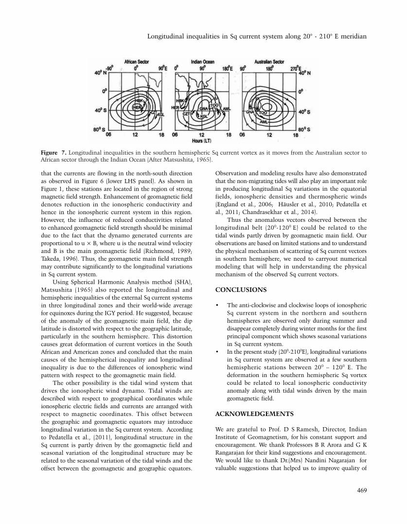
to study about the longitudinal inequalities, three different regions in southern hemisphere are considered with respect to geomagnetic longitude: zone-1- Australian sector, zone-2 -Indian ocean and zone 3 - African sector. the nature of sq vortex over Australian, Indian ocean and African sectors is shown in Figure 7. the southern sq vortex over the Australian sector appears to have normal oval shape but as it shifts its central position to Indian ocean, pole-ward side of the vortex undergoes significant deformation.
In the afternoon sector, the vortex tends to be stretched in n-s direction to produce n-s oriented current vectors at too and AML. In the morning sector, the current iso-lines deviate from north-West orientation to north-east orientation, to produce anomalous current vector pattern at HeR, CZt and KGL. the normal behavior of current vectors at HeR, CZt and KGL in the afternoon hours (expected sW orientations) suggest that deformed current vortex returns to normal oval shape as the central meridian of vortex transit from Indian ocean sector to the western part of Africa.
DISCUSSION
Ionospheric conductivity and tidal winds play an important role in the shape and strength of the sq current system (Richmond et al., 1976; takeda, 2013). thus, the seasonal and longitudinal differences in sq current system may be related to variations in conductivity or tidal winds or combination of the two. since the conductivity depends upon the geomagnetic main field strength, longitudinal variations in this field strength may introduce longitudinal differences in the sq current system (Matsushita, 1967). Modeling results have suggested that the conductivities associated with geomagnetic field variations can induce longitudinal variations in field aligned currents that are related to longitudinal differences in the hemispheric asymmetry of the sq current system (stening et al., 2007). In Figure 5, first principal component (PC-1) along the longitudinal band of 20o-120o e, denotes the anomalous behavior in H component at stations HeR, HBK, CZt, KGL and GnA as they do not show expected "V or inverted-V" type of pattern but show northern hemispheric type D-variations for summer (January) month. this indicates
Longitudinal inequalities in sq current system along 20° - 210° e meridian
469
that the currents are flowing in the north-south direction as observed in Figure 6 (lower LHs panel). As shown in Figure 1, these stations are located in the region of strong magnetic field strength. enhancement of geomagnetic field denotes reduction in the ionospheric conductivity and hence in the ionospheric current system in this region. However, the influence of reduced conductivities related to enhanced geomagnetic field strength should be minimal due to the fact that the dynamo generated currents are proportional to u × B, where u is the neutral wind velocity and B is the main geomagnetic field (Richmond, 1989; takeda, 1996). thus, the geomagnetic main field strength may contribute significantly to the longitudinal variations in sq current system.
Using spherical Harmonic Analysis method (sHA), Matsushita (1965) also reported the longitudinal and hemispheric inequalities of the external sq current systems in three longitudinal zones and their world-wide average for equinoxes during the IGY period. He suggested, because of the anomaly of the geomagnetic main field, the dip latitude is distorted with respect to the geographic latitude, particularly in the southern hemisphere. this distortion causes great deformation of current vortices in the south African and American zones and concluded that the main causes of the hemispherical inequality and longitudinal inequality is due to the differences of ionospheric wind pattern with respect to the geomagnetic main field.
the other possibility is the tidal wind system that drives the ionospheric wind dynamo. tidal winds are described with respect to geographical coordinates while ionospheric electric fields and currents are arranged with respect to magnetic coordinates. this offset between the geographic and geomagnetic equators may introduce longitudinal variation in the sq current system. According to Pedatella et al., (2011), longitudinal structure in the sq current is partly driven by the geomagnetic field and seasonal variation of the longitudinal structure may be related to the seasonal variation of the tidal winds and the offset between the geomagnetic and geographic equators.
observation and modeling results have also demonstrated that the non-migrating tides will also play an important role in producing longitudinal sq variations in the equatorial fields, ionospheric densities and thermospheric winds (england et al., 2006; Häusler et al., 2010; Pedatella et al., 2011; Chandrasekhar et al., 2014).
thus the anomalous vectors observed between the longitudinal belt (200-1200 e) could be related to the tidal winds partly driven by geomagnetic main field. our observations are based on limited stations and to understand the physical mechanism of scattering of sq current vectors in southern hemisphere, we need to carryout numerical modeling that will help in understanding the physical mechanism of the observed sq current vectors.
CONCLUSIONS
• the anti-clockwise and clockwise loops of ionospheric sq current system in the northern and southern hemispheres are observed only during summer and disappear completely during winter months for the first principal component which shows seasonal variations in sq current system.
• In the present study (200-2100e), longitudinal variations in sq current system are observed at a few southern hemispheric stations between 200 – 1200 e. the deformation in the southern hemispheric sq vortex could be related to local ionospheric conductivity anomaly along with tidal winds driven by the main geomagnetic field.
ACKNOWLEDGEMENTS
We are grateful to Prof. D s Ramesh, Director, Indian Institute of Geomagnetism, for his constant support and encouragement. We thank Professors B R Arora and G K Rangarajan for their kind suggestions and encouragement. We would like to thank Dr.(Mrs) nandini nagarajan for valuable suggestions that helped us to improve quality of
Figure 7. Longitudinal inequalities in the southern hemispheric sq current vortex as it moves from the Australian sector to African sector through the Indian ocean (After Matsushita, 1965).

s. K. Bhardwaj and P. B. V. subba Rao
470
the manuscript. We also thank Prof.B.V.s.Murthy for editing the manuscript.
Compliance with Ethical Standards
the authors declare that they have no conflict of interest and adhere to copyright norms.
REFERENCES
Alex, s., Kadam, B. D., and Rao, D. R. K., 1998. Ionospheric
current systems on days of low equatorial ΔH, J. Atmos.
solar-terr. Phys., v.60, pp: 371–379.
Alex, s., and Jadhav, M., 2007. Day-to-day variability in the
occurrence characteristics of sq focus during D-months
and its association with diurnal changes in the Declination
component, earth, Planets space, v.59, pp: 1197–1203.
Bhardwaj, s. K., and Rangarajan, G. K., 1998. A model for solar
quiet day variation at low latitude from past observations
using singular spectrum analysis, Proc. Indian Acad. sci.
(earth Planet sci.), v.107, pp: 217–224.
Bhardwaj, s. K., subba Rao, P. B. V., and Veenadhari, B., 2015.
Abnormal quiet day variations in Indian region along 75°
e meridian, earth, Planets space. (DoI :10.1186/s40623-
015-0292-1)., v.67, pp: 115.
Bhattacharyya, A., and okpala, K. C., 2015. Principal components
of quiet time temporal variability of equatorial and low-
latitude geomagnetic fields, J. Geophys. Res. space Physics,
doi:10.1002/2015JA021673., v.120, pp: 8799–8809.
Campbell, W. H., Arora, B. R., and schiffmacher, e. R., 1993.
external sq currents in the India-siberia region, J. Geophys.
Res., v.98, pp: 3741 – 3752.
Chandrasekhar, n. P., Arora, K., and nagarajan n., 2014.
Characterization of seasonal and longitudinal variability of
eeJ in the Indian region, J. Geophys. Res. space Physics,
doi:10.1002/2014JA020183., v.119, pp: 10,242–10,259.
Chapman, s., and Bartels, J., 1940. Geomagnetism, oxford
University Press, oxford., v. 1, pp: 613- 619.
Chulliat, A., Blanter, e. Le Mouel, J.-L. and shnirman, M.,
2005. on the seasonal asymmetry of the diurnal and
semidiurnal geomagnetic variations, J. Geophys. Res,
doi:10.1029/2004JA010551., v.110, pp: A05301 (1-14).
Cnossen, I., and Richmond, A. D., 2013. Changes in the earth’s
magnetic field over the past century: effects on the ionosphere-
thermosphere system and solar quiet (sq) magnetic
variation, J. Geophys. Res., DoI:10.1029/2012JA018447.,
v.118, pp: 849–858.
england, s. L., Maus, s., Immel, t.J., and Mende, s.B., 2006.
Longitudinal variation of the e-region electric fields caused
by atmospheric tides, Geophys. Res. Lett., 33, L21105,
doi:10.1029/2006GL027465.
Faynberg, e. B., 1975. separation of the geomagnetic field into
a normal and an anomalous part, Geomagn. Aeron., v.15,
pp: 117– 121.
Gurubaran, s., 2002. the equatorial counter electrojet: part of a
worldwide current system, Geophys. Res. Lett., v.29, pp:
1337 (51-1 to 51-4).
Häusler, K., Lühr, H., Hagan, M. e., Maute, A., and Roble R.
G., 2010. Comparison of CHAMP and tIMe GCM
nonmigrating tidal signals in the thermospheric zonal wind,
J. Geophys. Res., D00I08, doi:10.1029/2009JD012394.,
v.115.
IAGA working group 1975. IAGA Division I study Group, 1976.
International geomagnetic reference field 1975. eos trans.
Am. geophys. Un., v.57, pp:120-121.
Le sager, P., and Huang, t. s., 2002. Longitudinal dependence
of the daily geomagnetic variation during quiet time, J.
Geophys. Res., doi:10.1029/2002JA009287, v.107, pp:
1397(17-1 to 17-8).
Matsushita, s., 1965. Longitudinal and hemispheric inequalities
of the external sq current system. J. Atmos. terr. Phys.,
v.27, pp: 1317-1319.
Matsushita, s., 1967. solar quiet and lunar daily variation fields, in
Physics of Geomagnetic Phenomena, edited by s. Matsushita
and W.H. Campbell, chap. III-I, Academic, new York., pp:
301–424.
Matsushita, s., and Campbell W. H., 1967. solar quiet and lunar
daily variation fields. In: Physics of geomagnetic phenomena,
(new York: Academic press), v.1, pp: 301 – 424.
Matsushita, s., and Maeda, H., 1965. on the geomagnetic quiet
solar daily variation field during the IGY, J. Geophys. Res.,
v.70, pp: 2535 – 2558.
Patil, A., Arora, B. R., and Rastogi, R. G., 1985. seasonal variations
in the intensity of sq current system and its focus latitude
over the Indian region, Indian J. Radio space Phys., v.14,
pp: 131–135.
Pedatella, n. M., Forbes. J. M., and Richmond, A. D., 2011.
seasonal and longitudinal variations of the solar quiet
(sq) current system during solar minimum determined
by CHAMP satellite magnetic field observations, J.
Geophys. Res., doi:10.1029/2010JA016289., v.116, pp:
A04317.
Pham thi thu, H., Amory-Mazaudier, C., and Le Huy, M., 2011.
sq field characteristics at Phu thuy, Vietnam, during solar
cycle 23: comparisons with sq field in other longitude
sectors, Ann. Geophys., doi:10.5194/angeo-29-1-2011.,
v.29, pp: 1–17.
Price and Wilkins., 1963. new methods for the analysis of
geomagnetic fields and their application to the sq field of
1932-1933, Phil. trans. Royal society of London., v.A256,
pp: 31-98.
Rastogi, R.G., 1993. Disintegration of the ionospheric sq loop
system during winter solstices along 75o e longitude, Ann.
Geophys., v.11, pp: 40 – 46.
Richmond, A. D., Matsushita, s., and tarpley, J. D., 1976. on the
production mechanism of electric currents and fields in the
ionosphere, J. Geophys. Res., v.81, pp: 547 – 555.

Longitudinal inequalities in sq current system along 20° - 210° e meridian
471
Richmond, A. D., 1989. Modeling the ionosphere wind dynamo:
A review, Pure Appl. Geophys., v.47, pp: 413– 435.
schuster, A., 1889. the diurnal variation of terrestrial magnetism,
Philos. trans. Roy. soc. Lon., ser. A., v.180, pp: 467 – 518.
schuster, A., 1908. the diurnal variation of terrestrial magnetism,
Philos. trans. Roy. soc. Lon., ser. A., v.208, pp: 163 – 204.
shinbori, A., Koyama, Y., nose, M., Hori, t., otsuka, Y., and
Yatagai, A., 2014. Long-term variation in the upper
atmosphere as seen in the geomagnetic solar quiet daily
Variation, earth, Planets space., v.66, pp: 155 – 175.
stening, R. J., Reztsova, t., and Minh, L. H., 2007. Variation of
sq focus latitudes in the Australian/Pacific region during a
quiet sun year, J. Atmos. sol-terr. Phys., v.69, pp: 734–740.
sugiura, M., and Hagan, M.P., 1967. Universal-time changes in
the geomagnetic solar quiet daily variation sq, sci. Rep.,
GA-478, Washington University, seattle.
takeda, M., Yamada, Y., and Araki t., 1986. simulation of
ionospheric currents and geomagnetic field variations of sq for
different solar activity, J. Atmos. terr. Phys., v.48, pp: 277–287.
takeda, M., 1996. effects of the strength of the geomagnetic main
field strength on the dynamo action in the ionosphere, J.
Geophys. Res., v.101, pp: 7875 – 7880.
takeda, M., 2002. Features of global sq field from 1980 to 1990,
J. Geophys. Res., doi:10.1029/2001JA009210., v.107, pp:
sIA 4 – 8.
takeda, M., 2013. Contribution of wind, conductivity, and
geomagnetic main field to the variation in the geomagnetic
sq field, J. Geophys. Res., doi:10.1002/jgra.50386., v.118,
pp: 4516–4522.
torta, J. M., Marsal, s., Curto, J. J., and Gaya – Pique, L. R.,
2010. Behaviour of the quiet-day geomagnetic variation at
Livingston Island and variability of the sq focus position
in the south American-Antractic Peninsula region, earth,
Planets space., v.62, pp: 297 – 307.
Vertlib, A. B., and Wagner, C. U., 1970. Analysis of geomagnetic
sq variations by the expansion of fields in natural orthogonal
components I, Method and problems, Geomagn. Aeron.,
v.10, pp: 509–513.
Xu, W-Y., and Kamide, Y., 2004. Decomposition of daily
geomagnetic variations by using method of natural orthogonal
component, J. Geophys. Res., doi:10.1029/2003JA010216.,
v.109, pp: A05218.
Yamashita, s., and Iyemori, t., 2002. seasonal and local time
dependences of the inter-hemispheric field-aligned currents
deduced from the Ørsted satellite and the ground geomagnetic
observations, J. Geophys. Res., doi:10.1029/2002JA009414.,
v.107, no. (A11), pp: 1372.
Yamazaki, Y., and Yumoto, K., 2012. Long-term behavior of annual
and semi-annual sq variations., earth, Planets space., v.64,
pp: 417– 423.

U.Vadapalli and n.Vedanti
472
Time-lapse seismic response evaluation based on well log data for Ankleshwar reservoir, Cambay basin, India
U.Vadapalli* and N.VedantiCsIR – national Geophysical Research Institute, Hyderabad-500007, India
*Corresponding Author: [email protected]
AbSTRACTtime-lapse seismic reservoir monitoring can image fluid-flow effects in a reservoir if the changes in seismic properties of the reservoir due to production or on-going recovery processes are large enough to detect. thus, before acquiring a time-lapse seismic data, it is necessary to carry out feasibility study for time-lapse seismic reservoir monitoring to get an estimated seismic response. In the present study, Gassmann fluid substitution analysis and forward modeling based on well logs have been carried out to predict the seismic response of a paysand of Ankleshwar reservoir, which is being studied for Co2 – eoR. In this reservoir for enhanced oil recovery (eoR), Co2 injection into a paysand of the reservoir is found to be appropriate, taking into cognizance its success in different reservoirs all over the world.
the seismic response of paysand s5 in a well is modelled for different saturations and a variable thickness of Co2 in the paysand. It is observed that because of the first appearance of Co2, sudden drop in acoustic impedance of the paysand would lead to detectable time shift at the top. However, as Co2 occupies full thickness of the paysand time shift at the top is reduced. time shift at the bottom responds to overall velocity drop in full thickness of the paysand and it could not be detectable. We also inferred that in this case time-lapse time shift analysis would be more helpful compared to the amplitude analysis and it should be possible to image Co2 plume in the reservoir. the replacement of oil and water in the paysand with Co2 might lead to 9% drop in P-wave velocity.
Key words: time-lapse seismic response, Gassmann’s equation, fluid replacement modeling, well log data, Co2 injection, Co2 – eoR, Ankleshwar reservoir.
INTRODUCTION
A reservoir under production and enhanced oil Recovery (eoR) observes changes in saturation or pressure or both over the time. For many reservoirs, the effect of change in pore pressure will have a limited effect upon the seismic parameters (Landro 2002). Also the effect of pressure on reservoir properties is not yet fully established (Dimri et al., 2012). Changes due to saturation lead to considerable changes in seismic properties such as velocity, density and bulk modulus of the reservoir. Gassmann’s model (Gassmann 1951; Wang 2001; smith et al., 2003; Kumar and Mohan 2004; Mavko et al., 2009; Avseth et al., 2010; Dimri et al., 2012) is being mostly used to predict P and s wave velocities with respect to changes in saturation. the changes in seismic properties of the reservoir are being manifested on time-lapse seismic data either in the form of time shifts or amplitude variations or both. Depending upon the reservoir condition, data quality and repeatability issues, time-lapse amplitude analysis may or may not compliment the time-lapse time shift analysis. In the case of Gulfaks oil field in north sea, amplitude analysis is found to be more useful as compared to the time shift analysis (Landro et al., 1999). the aim of present study is to understand how would be the time-lapse seismic response of a paysand of the Ankleshwar reservoir in Cambay basin, India, which is a target for Co2 – eoR. In
pursuance of the same, synthetic seismic modeling based on well logs and Gassmann’s fluid substitution analysis is carried out to study the effect of saturation changes in synthetic seismic data. It is observed that the top of the reservoir will experience a detectable time shift after injection of Co2 into the reservoir and time-lapse time shift analysis would be more helpful compared to the amplitude analysis. the generation of synthetic sonic and density logs and synthetic seismic trace at variable saturations of Co2 is carried out by using Hampson-Russel software. the overall drop in P-wave velocity and P-impedance is estimated by using MAtLAB code for Gassmann’s fluid replacement analysis.
THE STUDy AREA
the study area, Ankleshwar oil field is one of the major oil producing fields of Cambay basin, India. In the field, tertiary sediments varying in thickness between 1343 and 2026 m have been deposited over Deccan trap basement (Mukherjee, 1981).the Ankleshwar formation, which is deposited in marine regression phase during Middle to Upper eocene age (Chowdhary 2004; Holloway et al., 2007), is a major reservoir unit in the field. the Ankleshwar reservoir consists of sandstone, shale and siltstone layers. the reservoir is subdivided into four major stratigraphic units viz., telwa shale, Ardol, Kanwa shale and
J. Ind. Geophys. Union ( september 2016 )v.20, no.5, pp: 472-481

time-lapse seismic response evaluation based on well log data for Ankleshwar reservoir, Cambay basin, India
473
Hazad members (Figure 1). the Ardol and Hazad members are recognized as sandstone units, however, they contain shale laminae in between. Hazad member hosts the main recoverable reserves of oil. Hazad and Ardol members together are divided into eight sand layers, viz., s1,s2, s3+4, s5, s6+7, s8+9, s10 and s11 from bottom to top. sand layer “s3+4” is the major producer in the field.
the field has been producing oil and gas since 1961. In 1966, the secondary recovery process, water injection was started to restore the declined reservoir pressure. now, the production has substantially declined and the water cut is more than 90%. the operator, oil and natural Gas Corporation (onGC) Ltd., has a strategy for Co2 – eoR to increase the life of field. A mixture of Co2 and other hydrocarbon gasses (methane, ethane, propane and butane) will be injected into paysands s3+4 and s5 for eoR. the vertical succession of s3+4, s5 sands and Kanwa interval in a well W6 is shown in Figure 2. the tops of these layers are taken from the formation evolution reports provided by the operator. the interpretation is mainly based on gamma ray log. the intervals with gamma ray counts less than 65 API and greater than 65 API represent sand layers and shale layers, respectively. As illustrated in Figure 2, the sand
layer s5 is subdivided into nine layers viz., s5-1, shale2, s5-2, shale3, s5-3, shale4, s5-4, shale5, s5-5 from bottom to top due to the presence of interbedded shale layers.
since reservoir modeling and simulation studies carried out by nGRI, India and sInteFF, norway (srivastava et al., 2012, Dimri et al., 2012) with support from onGC Ltd., India recommended the Ankleshwar reservoir for Co2 – eoR, we tried to do a feasibility assessment of time-lapse seismic to monitor Co2 that needs to be injected into the reservoir. We try to address the following questions based on Gassmann’s fluid substitution analysis and seismic forward modelling using well logs:
1. Can the changes in Ankleshwar reservoir due to replacement of oil and water with Co2 be manifested on time-lapse seismic data?
2. Will the changes in reservoir condition lead to either time-shift or amplitude variation in post injection seismic data?
3. Can the changes due to fluid replacement be detectable within the seismic resolution limit?
4. Will the time-lapse seismic monitoring of Co2
movement in this reservoir be feasible?
Figure 1. the generalized stratigraphy of the Cambay basin showing stratigraphy of the Ankleshwar formation (www.dghindia.org).

U.Vadapalli and n.Vedanti
474
Time-Lapse Seismic Response Evaluation for Ankleshwar Reservoir
to estimate the time-lapse seismic response of the reservoir after the replacement of oil and water in the reservoir with Co2, a well W6 drilled through s5 paysand is chosen for analysis as required sonic log was available for this well. the reservoir properties required for Gassmann’s fluid substitution analysis are taken from the production data and other information provided by the operator. According
to reservoir simulation result, initial water saturation at the time of Co2 injection is 60% (Ganguli et al., 2014). As the initial water saturation is 60% and since the reservoir has no gas cap (srivastava et al., 2012) the remaining 40% of pore space can contain oil. the average porosity of s5 sand layer is 24%, the irreducible water in the reservoir is 20% and residual oil saturation is 20% (information provided by the operator). thus, for the most feasible case out of 40%, only 20% of remaining oil can be produced using Co2 – eoR. Injection of Co2 increases oil production
Figure 2. the vertical succession of Kanwa interval, s5 sand, shale1 and s3+4 sand layers identified on gamma ray, density and sonic logs of well W6. Dark intervals represent shale laminae. the sublayers of the s5 sand layer are also demarcated on the figure.

time-lapse seismic response evaluation based on well log data for Ankleshwar reservoir, Cambay basin, India
475
and reduces water production. out of the 40% producible water, on an average 15% will be produced (Ganguli et al., 2014) after Co2 injection. thus, Co2 has to replace 20% oil and 15% water, hence the maximum Co2 saturation in the sand layer can be 35%.
the physical properties of Co2 with reservoir condition of s5 sand layer at 75oC temperature and 121.6kg/cm3 pressure are computed using Batzle and Wang (1992) equations. since s-wave velocity information is not available, dry rock poisson’s ratio 0.1 is used for computation of dry rock modulus or frame bulk modulus (Kd). For computation of the matrix bulk modulus (Km), composition of s5 sand layer (Figure 2) is considered as 90% quartz and 10% clay. the physical properties of s5
sand layer used in fluid substitution modeling are given in table 1.
Injected Co2 accumulates under the cap of the reservoir and thickens downward by replacing insitu fluids. thus, the effect of variation in thickness as well as saturation is studied. the liquids in s5 sand layer are systematically replaced by Co2 in steps of 5% increase in saturation. the thickness of Co2 in the target zone has gradually increased downward from 0 m to 18 m in steps of 3 m. the target zone is 18 m thick (top at 1176m and bottom at 1194m) (Figure 2), which means Co2 gas has occupied entire paysand. to carry out forward modeling, velocity and density structure of the reservoir at initial saturation conditions is available from the sonic and density logs. For each value of Co2 saturation,
Figure 3. the figure illustrates the abrupt drop in saturated bulk modulus, P-wave velocity and P-impedance until Co2 saturation is 15%.

U.Vadapalli and n.Vedanti
476
synthetic sonic and density logs are generated. to monitor the seismic response of the paysand s5 with changes in fluid saturation, a Ricker wavelet of 50 Hz frequency is convolved with reflectivity series and zero offset synthetic seismic traces are generated. the synthetic seismic traces generated without Co2 in the paysand are considered as baseline data. synthetic seismograms generated for varying saturation and for different thicknesses of Co2 in the reservoir represent monitor data.
to estimate the average velocity drop in the s5 sand layer, an average value of 2774 m/s obtained from sonic log is used as initial P-wave velocity for Gassmann fluid substitution analysis using MAtLAB code. A Change in P-wave velocity, P-impedance and bulk modulus with the
increase in Co2 saturation is studied. the percentage drop in P-wave velocity and P-impedance of the paysand s5, due to replacement of oil and water with Co2 is estimated.
RESULTS
steep drop in saturated bulk modulus, P-wave velocity and P-impedance is observed until Co2 saturation reaches 15%. After that stage variation in these quantities is subtle (Figure 3). As Co2 saturation reaches 35%, P-wave velocity drops by 9% and P-impedance drops by 10%. Figure 4 illustrates the baseline seismic data, which represents the paysand without Co2. Figure 5 illustrates the synthetic seismic data sets modeled at variable saturations of Co2
Figure 4. Baseline seismic data (a single trace is repeated many times in order to display it as data) generated from the initial values of saturation in the paysand. Gray scale represents P-wave velocity. top of s5, top of shale 1 and top of s3+4 are shown on synthetic data with horizontal lines.
Table 1. the physical properties of s5 sand layer used for analysis
Parameter Value
Reservoir temperature 75oC
Reservoir pressure 121.6 Kg/cm2
Bubble Point Pressure 90.5 Kg/cm2
Water saturation 60%
oil saturation 40%
Bulk modulus of oil 1 GPa
Bulk modulus of water/brine 2.38GPa
Bulk modulus of Co2– gas 0.06149Gpa
Density of oil 750 Kg/m3
Density of water/brine 1090 Kg/m3
Density of Co2 - gas 373 Kg/m3

time-lapse seismic response evaluation based on well log data for Ankleshwar reservoir, Cambay basin, India
477
Figure 5. Modeled P-wave velocity with gray scale and synthetic seismic traces for varying saturation and thickness of Co2; a-f represent monitor data with 3 m, 6 m, 9 m, 12 m, 15 m and 18 m thickness of Co2, respectively. Figure 5a clearly shows 6 ms time shift of the top compared to the baseline case (Figure 4). Figure 5e shows 2 ms time shift at the top and bottom of s5 layer and at the top of s3+4. Figure 5f reveals that top of shale 1 interferes with the top of s3+4 as Co2 occupies full thickness of the sand layer. Figures 5d and 5e show a sub horizontal reflector between top_s5 and top_shale 1.

U.Vadapalli and n.Vedanti
478
in the paysand. In Figures 4 and 5, background gray scale represents modeled P-wave velocity. As shown in Figure 5a to Figure 5e, in the time window 580 ms to 598 ms, darker region decreases with increase in saturation, which indicates a drop in velocity with Co2 saturation in the target zone. this velocity drop leads to the reduction in acoustic impedance difference between Kanwa shale and s5-5 sand layer and also between s5-1 sand and shale 1 (Figure 2). At initial saturation conditions, i.e. without Co2 in the paysand, the top reflector of the paysand (top_s5) is at 580 ms and the bottom reflector (top_shale1) is at 592 ms (Figure 4). After the first appearance of Co2 in the paysand, i.e. when it occupies 3 m thickness of the paysand, the top reflector is pushed down by 6 ms and the bottom reflector (shown as top_shale1 on Figure 5a) is pushed down by 2 ms. However, as gas thickness increases in the paysand, time shift at the top reservoir reduces to 2 ms (Figures 5d-f). Careful observation of Figure 5d and Figure 5e shows another sub-horizontal reflector at the bottom of Co2 plume, which is between top of s5 and top of shale 1. As illustrated in Figure 5f, when Co2 had occupied entire paysand, top_shale1 has interfered with top_s3+4.
DISCUSSION
Replacement of oil and water in the s5 paysand of the Ankleshwar reservoir with Co2 using Gassmann’s equation and available information infers that there could be 9% drop in P-wave velocity for 35 % of Co2 saturation. the injection of Co2 into s5 paysand can cause substantial changes
in bulk modulus, the P-wave velocity and P-impedance until its saturation reaches 15%. the variation in these quantities becomes subtle beyond 15% saturation. the synthetic seismic modeling exercise carried out for the s5 sand layer in a well (W6) of Ankleshwar reservoir predicts that injection of Co2 into the paysand will lead to push down effect at the top and the bottom of the reservoir. However, fluid replacement effect will be more visible at the top reflector and should give rise to observable time shift (6 ms) on the real time-lapse seismic data. Due to the first appearance of Co2 in the topmost 3 m of the paysand there will be 6 ms push down effect at the top. In the present study, the push down effect at the top is due to the reduction in the acoustic impedance of the paysand with respect to overlying Kanwa shale formation. the actual top of the paysand at 580 ms on baseline data could be mapped at 586 ms on monitor data, because acoustic impedance difference is large enough to cause a reflection at 586 ms. the reflection event at 586 ms can be considered as apparent top of the paysand “s5”. However, as gas occupies full thickness of the paysand, the time shift at the top reduces to 2 ms (Figure 5 d-f). Hence, we can infer that the first monitor survey should be acquired before Co2 occupies full thickness of the paysand. the maximum time shift at the bottom of the paysand s5 is only of the order of one sample (2 ms) (Figure 5 c-f) and also the bottom reflector (top-shale 1) interferes with the top of the sand layer “s3+4” (Figure 5f), when Co2 occupies full thickness of the paysand. thus, the time shift of the bottom of the paysand may not be resolved in real time-lapse seismic
Figure 6. the cross-correlation output of base data with monitor data representing the paysand occupied by 3m thickness of Co2. the cross-correlation peak is at 6 ms.

time-lapse seismic response evaluation based on well log data for Ankleshwar reservoir, Cambay basin, India
479
Figure 7. Cross-correlation output of base data with monitor data sets modeled at 3 m, 6 m, 9 m, 12 m, 15 m and 18 m thickness of Co2 inside the s5paysand. In Figure a cross-correlation peak is at 2 ms and in b-f cross-correlation peak has gradually moved towards 0 ms.

U.Vadapalli and n.Vedanti
480
studies. the drop in acoustic impedance difference of the paysand with respect to Kanwa shale and shale1 layers due to injection of Co2 will lead to a reduction in amplitude of top reflector. thus, in this case time-lapse amplitude analysis may not be much helpful. Below the Co2 plume a sub-horizontal reflection occurs due to acoustic impedance contrast between the Co2 saturated paysand and the remaining paysand. this sub horizontal reflector would help to monitor Co2 movement in the reservoir.
In the absence of data from major paysand s3+4, this analysis was carried out for another paysand s5. If the operator injects Co2 into the sand layer “s3+4”, similar results will be generated because similar to the sand layer “s5”, the s3+4 sand layer is also overlaid by a lower velocity shale layer (shale 1). thus, in this case also injection of Co2 will lead to reduction in acoustic impedance difference between s3+4 sand layer and shale 1 layer and amplitude analysis may not be helpful in detecting time-lapse changes. the maximum time shift 6 ms at the top of s5 paysand is due to the first appearance of Co2 in high velocity, s5-5 sub layer (Figure 2), which is underlain by low velocity shale 5 sublayer. such kind of velocity sub layering inside s5 sand layer made fluid substitution effect more prominent at the top. In case of sand layer “s3+4” there is no such velocity sub layering, thus, the magnitude of time shift at the top might be lower than that of s5 sand layer. the sub layers inside s5 sand layer could not be detected on synthetic seismic section. the velocity sub layering detected on sonic log could add additional information for the interpretation.
In the present study, synthetic modeling is carried out at a single well because of the limited information available. We are aware that for a comprehensive evaluation, synthetic modeling should be done for the entire reservoir for estimation of time shifts. We also believe that real data will be different from the synthetic one because of noise and other assumptions. the noise in real data may obscure the sub-horizontal reflector below the Co2 plume and it might go undetected. We have seen that maximum changes are observed at 15% gas saturation, but it would be interesting to estimate the time Co2 plume will take to attain 15% saturation.
the quality check of the results is performed. Base data is cross correlated with the monitor data sets to verify time shift at the top and bottom of the paysand s5. Cross-correlation of baseline data with monitor data modeled for the paysand occupied by 3 m thick Co2 is done in time window of 570 ms to 590 ms, which covers the top reflector of the paysand. In Figure 6 the cross-correlation peak is at 6 ms, which infers that due to the first appearance of Co2, the top of the paysand is pushed down by 6 ms. In order to quantify the time shift at the bottom of the s5
paysand, cross-correlation of base and monitor data sets is done in the time window covering whole paysand, time
window 570 ms to 600 ms. Figures 7a-f represent the cross-correlation outputs for 3 m, 6 m, 9 m, 12 m, 15 m and 18 m thick Co2 plume in the s5 paysand. In Figure 7a the central cross-correlation peak is at 2 ms, which represents that bottom of the paysand was pushed down by 2 ms, when Co2 had occupied 3 m thickness of the paysand. As illustrated in Figure 7b-f with increase in thickness of Co2 in the paysand, the central cross-correlation peak has gradually moved towards zero. In Figures 7a-f time shift is maximum at maximum Co2 saturation.
the observed time shift at the bottom of the paysand is verified from the observed velocity drop (9% of the initial velocity) using the empirical relation developed by Landrø and stammeijer (2004). the relation between relative time shift and relative velocity drop is given as:
Dt – DV ––– = ––––– ................ (1) t VWhere, V is the initial average velocity of the reservoir, ΔV is the velocity drop and t is the two way time thickness of the paysand, which is given as below
2Z t = ––––– ................ (2) VWhere, Z is the thickness of the zone. After the substitution of initial velocity and estimated velocity drop into the above equations the theoretical time shift is found to be 2 ms. The theoretically predicted time shift (ΔT) at the bottom of the paysand, 2 ms matches with the observed value on synthetic seismic data.
CONCLUSIONS
Injection of Co2 under miscible conditions into the s5 sand layer of the Ankleshwar reservoir will lead to detectable time shift at the top. the time-lapse time shift analysis would be more helpful as compared to the time-lapse amplitude analysis for detection of time-lapse changes, as fluid substitution leads to reduction in acoustic impedance difference. the monitor seismic survey would image Co2 plume as a sub-horizontal reflector below Co2 saturated sand. Hence, time-lapse seismic monitoring of injected Co2 in the Ankleshwar reservoir is feasible.
ACKNOWLEDGEMENT
the authors are thankful to the Director, CsIR-nGRI for permission to publish this work. they are indebted to norwegian embassy, new Delhi for financial support through Indo-norwegian research project. they thank onGC Ltd., India for providing data to carry out this work. Useful suggestions by reviewers and Chief editor are gratefully acknowledged.

time-lapse seismic response evaluation based on well log data for Ankleshwar reservoir, Cambay basin, India
481
Compliance with Ethical Standards
the authors declare that they have no conflict of interest and adhere to copyright norms.
REFERENCES
Avseth, P., Mukerji, t., and Mavko, G., 2010. Quantitative
seismic interpretation: Applying rock physics tools to reduce
interpretation risk. Cambridge University Press.
Chowdhary, L. R., 2004. Petroleum Geology of the Cambay Basin,
Gujarat., India. Indian Petroleum Publishers.
Dimri, V., srivastava, R. P., and Vedanti, n., 2012. Fractal models
in exploration geophysics: applications to hydrocarbon
reservoirs, elsevier., v.41.
Ganguli, s. s., Vedanti, n., Akervoll, I., and Bergmo, P., 2014,
January. An estimation of Co2-eoR Potential from a sector
model in a mature oil field, cambay Basin, India. In Annual
convention, IGU-Kurukshethra, 2014.
Gassmann, F., 1951. Über die elastizität poröser medien:
Vierteljahrss-chrift der naturforschenden Gesellschaft in
Zurich. Paper translation at http://sepwww. stanford. edu/
sep/berryman/Ps/gassmann. pdf., v.96, pp: 1-23.
Holloway, s., Garg, A., Kapshe, M., Pracha, A.s., Khan, s.R.,
Mahmood, M.A., singh, t. n., Kirk K.L., Applequist, L.R.,
Deshpande, A., evans, D.J., Garg, Y., Vincent, C.J., and
Williams, J.D.o., 2007. A regional assessment of the potential
for Co2 storage in the Indian subcontinent, sustainable
and Renewable energy Programme Commissioned Report
CR/07/198 by British Geological survey (BGs). sustainable
and Renewable energy Programme Commissioned Report
CR/07/198, British Geological survey (BGs), neRC.
Kumar, A., and Mohan, s., 2004. Feasibility Assessment of a
time-Lapse seismic survey for thermal eoR in Balol Field,
India, Based on Rock Physics and seismic Forward Modeling.
In Proceedings of the 5th International Conference and
exposition on Petroleum Geophysics, society of Petroleum
Geophysicists, pp: 688-695.
Landrø, M., solheim, o. A., Hilde, e., ekren, B. o., and strønen,
L. K., 1999. the Gullfaks 4D seismic study. Petroleum
Geoscience, v.5, no.3, pp: 213-226.
Landrø, M., 2002. Uncertainties in quantitative time-lapse
seismic analysis.Geophysical Prospecting, v.50, no.5, pp:
527-538.
Mavko, G., Mukerji, t., and Dvorkin, J., 2009. the rock physics
handbook: tools for seismic analysis of porous media.
Cambridge university press.
Mukherjee, M. K., 1981. evolution of Ankleshwar anticline,
Cambay Basin, India.
smith, t. M., sondergeld, C. H., and Rai, C. s., 2003. Gassmann
fluid substitutions: A tutorial. Geophysics, v.68, no.2, pp:
430-440.
srivastava, R. P., Vedanti, n., Dimri, V. P., Akervol, I., Bergmo, P.,
and Biram, R. s., 2012, november. Co 2-eoR: A Feasibility
study of an Indian oil Field. In 2012 seG Annual Meeting.
society of exploration Geophysicists.
Wang, Z., 2001. Fundamentals of seismic rock physics. Geophysics,
v.66, no.2, pp: 398-412.

M.s. Chaudhari, M. Majumder, V. Bagade and s. Ranga
482
Assessing Quality of Masonry Dam using Seismic and Electrical Tomography
M.S. Chaudhari*, M. Majumder, V. bagade and S. RangaCentral Water and Power Research station, Pune-411024, Maharashtra, India
*Corresponding Author: [email protected]
AbSTRACTthe ageing and degradation of dam structures is an inevitable problem and its consequences on the safety of the structure are important. Presently, site characterization using geotechnical engineering has some limitations to adequately describe the subsurface ground conditions. All geotechnical tests provide information from point to point and the values are interpolated in between places. these tests grossly under sample the subsurface and are frequently inadequate. Geophysical methods are useful as non-destructive tools that can provide information over large volumes as compared to point measurements. the use of seismic tomography and electrical resistivity imaging in the assessment of dam structure is very apt and useful. seismic tomography survey was carried out in five horizontal and two vertical planes in the body of the Manikdoh masonry dam and one electrical resistivity imaging profile was taken on the top of the dam. the travel time data for tomography analysis was collected by placing geophones on the downstream face and hammer points on the upstream face of the dam. the compressional (P-) wave velocity distribution between each consecutive pair of source line and receiver line of the plane was computed using simultaneous Iterative Reconstruction technique. the weak zones, if present, reveal low P- wave velocity values and hence can be delineated. the reliability of travel time data is ensured by comparing the P- wave velocities at the point of intersection of common source to receiver pairs in horizontal and vertical planes. the tomography survey results revealed that the low velocity zones (velocity ranging between 1500 m/s to 2500 m/s) are between elevations 695 m to 705 m from chainage 463 m to 469 m. the four weak zones obtained from the horizontal planes matched well with that in vertical tomograms. Further, these low velocity zones are supported by presence of low resistivity patch (resistivity ranging between 129 Ω m to 829 Ω m) between elevation from 697 m to 693 m from chainage 462 m to 474 m in electrical resistivity imaging section.
Key words: seismic tomography, dam safety, masonry dam, Imaging
INTRODUCTION
Assessing the quality of dam structure is important to ensure its integrity and stability. seismic tomography has been used extensively in geophysical work (Dines and Lytle, 1979), e.g. for a dam site on Reunion Island (Cotton et al., 1986), for research on buried voids, for shafts and tunnels (Lytle and Dines, 1980) and for Pre-and Post-excavation studies for a nuclear power plant (Wadhwa et al., 2005). In tomographic reconstruction, seismic energy, which has propagated through a medium, is measured and from this energy, internal distribution of amplitude, phase shift or travel time observations (acoustic tomograms) are obtained by inversion process (Redington and Berninger, 1982; Jackson and tweeton, 1994). seismic tomography (using travel time data) and electrical tomography surveys were carried out in the present study for assessing the quality of a masonry Dam.
Manikdoh dam is a masonry dam with a height of 53 m and length of 927.05 m, constructed on River ‘Kukadi’ in Junnar taluka of Pune District in the year 1984 which has a total storage capacity of 308.06 M.cum (10.88 tMC). subsequent to the impoundment of the dam, heavy leakages were observed through the masonry in both the galleries as well as in the downstream face of the dam.
In view of this, seismic straight ray travel time tomography of the structure was carried out to suggest possible weak zones which are susceptible for seepage. seismic tomography survey was carried out along five horizontal and two vertical planes in the month of May when the water level in the reservoir was minimum. the quality of in-situ masonry is an important parameter and can be assessed by seismic wave method as the compressional wave velocities evaluated by this technique give an idea of the strength of the masonry. the velocity distribution, in turn helps in delineating the lateral and vertical extent of weak zones by anomalous velocity values. electrical Resistivity Imaging was carried out across one profile using 48 electrodes with 2 m spacing on the top of the dam.
METHODOLOGy
Seismic Tomography
seismic wave tomography was carried out with the help of a 10 Kg sledge hammer at preset locations on the upstream face of the dam while the seismic wave arrivals were picked up by different detectors (geophones of 10 Hz
J. Ind. Geophys. Union ( september 2016 )v.20, no.5, pp: 482-489

Assessing Quality of Masonry Dam using seismic and electrical tomography
483
frequency) placed on the downstream face of the dam at known locations. the seismic arrivals were amplified and recorded on a 24-channel signal enhancement seismograph Mcseis sX. the survey was conducted along five horizontal planes at elevations 705 m, 700 m, 695 m, 690 m, 685 m and two vertical planes at chainage 463 m and 443 m (Figure 1). the hammer points were located at the same elevation of geophones but on the upstream face of the dam. In horizontal planes, 24 geophones spaced 2 m apart were placed on the downstream face of the dam and 47 hammer points spaced 1 m apart were used for generating acoustic waves on the upstream face of the dam yielding 1128 ray paths. typical ray paths between 12 positions
of the hammer (source line) on the upstream face and 12 positions of geophones (receiver line) on the downstream face of the dam are shown in Figure 2. the first plane was at RL 705 m and other four planes were at 5 m elevation difference successively.
In vertical planes taken across the dam axis, 24 geophones spaced 1 m apart were placed on the downstream face of the dam and 24 hammer points spaced 1 m were used for generating acoustic waves on the upstream face of the dam yielding 576 ray paths. the geophones were planted vertically on the tip of the metallic rod inserted at the desired location by drilling small drill hole for maximum sensitivity.
Figure 1. schematic diagram showing horizontal and vertical planes covered by seismic tomography survey
Figure 2. typical ray diagram for various positions of source and receiver.

M.s. Chaudhari, M. Majumder, V. Bagade and s. Ranga
484
the travel times of these arrivals were measured from the seismic record on which a time scale is maintained. From the measured time of first arrival of the seismic waves and the distance between source (hammer point) and the receiver (geophone), the average velocity of propagation of the elastic wave for that distance was calculated. the recorded wave arrival data were analyzed by seismic ray tomography which enables the imaging of the velocity distribution within the sampled area. In this analysis, the area under study is divided into pixels, the number and size of which depend upon the number of ray paths and size of the area traversed. the data were analyzed using the algorithm of Jackson et al., (1992). From the velocity distribution, weak zones were delineated.
Electrical Resistivity Imaging
the electrical resistivity imaging survey was conducted by ARes automatic resistivity imaging system on one profile with Wenner-schlumberger array with 48 electrodes spaced at 2 m interval on the top of the dam from chainage 432 m to 526 m. the apparent resistivity values thus measured were inverted using Res2DInV software package to obtain true resistivity depth section.
Data Analysis
Data analysis was done using ‘MIGRAtoM’ (algorithm of Jackson et al., 1992) software. the seismic tomography of the dam across the zone between the receiver line on the downstream face and source line on the up-stream side of the dam which was divided into small pixel depending on the total number of P-wave arrivals recorded in the field experiment. the two dimensional plane 1-1 at elevation 705 m (Figure 1) between source line and receiver line was discretised on square grid points, 14 across the width of the plane (0.552m) and 47 along the plane (1.0 m). In the procedure adopted for data collection, there were 1128 rays and hence 1128 travel time equations. the number of pixels for this plane was 658. this means 658 unknowns against 1128 equations. It is possible to solve this type of problem through a near unique inversion. once the pixel size is decided, tomographic inversion begins with an assumption of initial model of the P- wave velocity between
source line and receiver line. With these initial average velocities, first arrival times of the rays for all possible positions of sources and receivers were calculated using straight ray tracings. these synthetic travel times were compared with the field measured travel times and the differences or residuals inverted to obtain perturbations to the velocity model using algorithm of Jackson et al., (1992). the procedure was repeated and the velocity model refined until, either there are no differences between the model travel times and the measured arrival times or RMs error was within the set limit (singh and singh, 1991). travel time data for tomographic analysis was collected on one plane at a time.
the seven tomograms depicting P wave velocity distribution were obtained by inverting the arrival times. the reliability and uniqueness of the velocity tomograms were improved by taking the lower (1000 m/sec) and upper (4000 m/sec) limits of the velocities depending on wave velocities of different masonry reported in the literatures (Forde and Batchelor, 1994; Camplani et al., 2008) and are given in table 1. Analysis of synthetic model studies suggests that the upper and lower velocity limits are helpful in obtaining a velocity distribution that is unique and matches more closely with the model data (Ghosh et al., 2000).
Resistivity imaging data analysis was done using Res2DInV software. the electrical resistivity depth section was obtained by plotting true resistivity values against depth. the electrical resistivity of saturated, unconsolidated sediment and rocks are controlled by porosity, grain size, morphology of pore space and resistivity of the pore fluid. the range of resistivities for the stone masonry is very large extending from 10 Ω m to 10000 Ω m (RILEM TC 127-MS, 2001). In the model studies carried out in saturated and dry rubble masonry (Flint et al., 1999) resistivity shows a variation from 200 Ω m to 2000 Ω m respectively.
RESULTS AND DISCUSSION
Seismic Tomography
the five horizontal and two vertical tomograms depicting lateral and vertical variations of P-wave velocities for the planes between source lines on the upstream side and
Table 1. P-Wave velocity for different types of masonry (from table 2 of Forde, and Batchelor, 1994)
sr. no. Material Av. sonic Velocity (m/s) source
1 Granite masonry Pier no 1 3450 Birjandi,1986
2 Granite masonry Pier no 2 3370 Birjandi,1986
3 Red sandstone masonry Pier 1970 Birjandi,1986
4 Yellow sandstone masonry Pier 2040 Birjandi,1986
5 Whinstone masonry Pier 2500 Birjandi,1986
6 White sandstone Pier 1700 Birjandi,1986

Assessing Quality of Masonry Dam using seismic and electrical tomography
485
receiver lines on the downstream side were obtained by inverting the arrival times using algorithm of Jackson et al., (1992).
During the analysis, the lower velocities observed very close to source and receiver lines were ignored. this is because these lower velocities may be due to ray density being less, close to the source and receiver locations or due to actual weak zones or their combinations. As it is
not possible to separate the contribution of these factors, it is recommended that weak zones observed very close to the source and receiver locations be ignored. tomograms depict contoured image of the P-wave velocities in grey scale, showing low velocity region in light grey colour and high velocity region in dark grey colour.Figure 3 shows a low velocity zone W 1 with velocity range 2000 to 2500 m/sec observed from chainage 441 m to 444
Figure 3. P- wave velocity distribution along plane P 1-1 (705-705) m elevation
Figure 4. P- wave velocity distribution along plane P 2-2 (700-700)

M.s. Chaudhari, M. Majumder, V. Bagade and s. Ranga
486
m on the upstream side extending from 2 m to 4.5 m across the plane 1-1. similarly Figure 4 shows the P-wave velocity distribution for plane 2-2 at 700 m elevation. this plane appears to have a velocity above 2500 m/s. An isolated low velocity zone W 2 (velocity ranging from 1500 to 2500 m/sec) can however be spotted from chainage 463 m to 468 m on the upstream side and extending from 0 m to 2 m across the width of the plane.
P-wave velocity distribution for plane 3-3 at 695 m elevation is depicted in Figure 5. A very prominent low velocity zone W 3 with velocity ranging from 1500 m/sec
to 2500 m/sec is observed from chainage 462 m to 469 m extending from 0 m upstream to 4 m towards downstream. the remaining part of the plane shows a velocity above 2500 m/s indicating good quality masonry.
P-wave velocity distribution for plane 4-4 at 690 m elevation and for plane 5-5 at 685 m elevation shows high values of P-wave velocity (ranging from 2500 m/s to 4000 m/s) indicating good quality masonry along the entire planes. so, no weak zone was attributed to these planes.
Figure 6 depicts the P-wave velocity distribution of vertical plane VP-1 at chainage 443 m spanning the
Figure 5. P- wave velocity distribution along plane P 3-3 (695 – 695)
Figure 6. P- wave velocity distribution along vertical plane VP 1 at chainage 443 m

Assessing Quality of Masonry Dam using seismic and electrical tomography
487
elevation range 685 m to 708 m. A low velocity zone W 4 with velocity ranging from 1500 m/s to 2500 m/s is seen from elevation 702 to 705 m and extending laterally from 0 m upstream to 5 m downstream. the rest of the plane shows velocities above 2500 m/s suggesting good quality masonry. this low velocity zone W 4 may be correlated with the low velocity zone W 1 found in plane P 1-1 (Figure 3) from chainage 441 m - 444 m at elevation 705 m.
Figure 7 depicts the P-wave velocity distribution of vertical plane VP-2 at chainage 463 m extending from elevation range 685 m to 708 m. two low velocity zones with velocity ranging from 1500 m/s to 2500 m/s are seen on the upstream side. the first low velocity zone W 5 is spotted from eL 700 m to 703 m on the upstream side dipping down towards downstream and tapering off at eL 697.5 m extending 8 m towards downstream. the second low velocity zone W 6 is observed from elevation 693 m to 698 m at upstream face dipping down towards downstream and tapering off at elevation 692 m extending for 8 m from upstream to downstream.
Electrical Resistivity Imaging
one electrical resistivity imaging section of 94.0 m length taken on the top of the dam at elevation 714.3 m from chainage 432 m to 526 m using Wenner-schlumberger electrode configuration is shown in Figure 8. From the section it is seen that one low resistivity zone with resistivity ranging from 129 Ω m to 829 Ω m exists from chainage 462 m to 474 m corresponding to elevation from 700 m to 696 m. this low resistivity zone corroborates with the low velocity zone W 3 obtained in horizontal plane 3-3 at elevation 695 m.
Correlation of weak zones
the correlation studies of low velocity zones observed in different tomograms indicates that the low velocity zone W 1 at Plane 1-1 (Figure 3) coincides with low velocity zone W 4 observed in Plane VP-1 (Figure 6) between elevation 702 m to 705 m and within chainage 441 m to 443 m.
Table 2. Correlation of weak zones observed in different seismic tomograms taken at different section of the Dam
Sl. No Plane No Weak Zones Elevation (m) Chainage (m) Description
1 P 1-1 W 1 705 441-444 2 to 4.5 m across the plane
2 P 2-2 W 2 700 463-468 0 to 2 m across the width of the plane
3 P 3-3 W 3 695 462-469 0 to 4 m across the width of the plane
4 VP-1 W 4 702-705 443 extending laterally from 0 – 5m
5 VP-2 W 5 700-703 463 Dipping downwards to the downstream and tapering off at eL 697 m.
6 VP-2 W 6 693-698 463 Dipping downwards to the downstream and tapering off at eL 692 m.
Figure 7. P- wave velocity distribution along vertical plane VP 2 at chainage 463 m

M.s. Chaudhari, M. Majumder, V. Bagade and s. Ranga
488
Figure 8. electrical Resistivity Imaging section from chainage 432 m to 526 m.
Figure 9. Correlation of electrical Resistivity Imaging section with seismic tomograms obtained at different elevations.
the correlated weak zone W 4 has a lateral extension of approximately 4 m. Further correlation indicates a weak zone of relatively greater extension at planes P 2-2, P 3-3 and VP-2.
the low velocity zone W 2 observed at Plane P 2-2 (Figure 4) occurring within chainage 463 m to 468 m can be correlated with the low velocity zone W 3 in plane 3-3 (Figure 5). these zones further can be correlated with two low velocity zones W 5 and W 6 observed in plane VP- 2 (Figure 7) at elevation between 693 to 703 m. the tabular presentation has been prepared for better view of correlation and is shown in table 2.
Results obtained from seismic tomography survey were further compared with electrical resistivity imaging section of 94.0 m length taken on the top of the dam at elevation 714.3 m from chainage 432 m to 526 m (Figure 9). A relatively low resistivity zone with resistivity ranging from 129 Ω m to 829 Ω m has been observed from chainage 462 m to 474 m at elevation from 697 m to 693 m. this resistivity range corresponds to saturated masonry (RILeM tC 127-Ms, 2001; Flint et al., 1999). this low resistivity zone also correlates with the low velocity zones W 2, W 3, W 4, W 5 found in tomograms of Plane 2-2, Plane 3-3 and vertical plane VP-2 respectively.
CONCLUSIONS
the tomography survey results suggest that the possible low velocity zones lie between elevations 695 m to 705 m. two low velocity zones W 2 & W 3 in the horizontal plane P 2-2 and P 3-3 are further supported by the low velocity zone W 5 and W 6 obtained from vertical section VP-2 at elevation 700 m to 703 m and 693 m to 698 m. therefore, the prominent low velocity zone extending from elevation 695 m to 703 m from chainage 462 m to 469 m is inferred to be a weak zone. From the electrical Resistivity Imaging section, it is observed that one low resistivity zone with resistivity ranging from 129 Ω m to 829 Ω m from chainage 462 m to 474 m at elevation from 697 m to 693 m corroborates with the low velocity zone W 2, W 3, W 4, W 5 found in tomograms of Plane 2-2, Plane 3-3 and vertical plane VP-2 respectively at elevation 695 m. these weak zones are susceptible for seepage and can be selectively treated.
ACKNOWLEDGEMENTS
Authors are grateful to Dr. M. K. sinha, Director, Central Water and Power Research station (CWPRs), Pune for constant encouragement and for permission to publish

Assessing Quality of Masonry Dam using seismic and electrical tomography
489
this paper. the help and co-operation extended by project authorities during collection of data is thankfully acknowledged. Authors are thankful to Dr. M.R.K. Prabhakar Rao for useful suggestions. they also express thanks to B.V.s. Murthy for useful suggestions and editing.
Compliance with Ethical Standards
the authors declare that they have no conflict of interest and adhere to copyright norms.
REFERENCES
Birjandi, F. K., 1986. sonic investigation of masonry structures,
Ph.D. thesis, University of edinburgh.
Camplani, M., Cannas, B., Carcangiu, s., Concu, G., Fanni,
A., Montisci, A., and Mulas, M. L., 2008. Acoustic
tomography for non destructive testing of stone masonry,
springer-Verlag Berlin Heidelberg, Part II, LnCs 5073,
pp: 596-605.
Cotton, J.F., Deletie, P., Jacquet – Francillon, H., Lakshmanan, J.,
Lemeine, Y., and sanchez, M., 1986. Curved ray seismic
tomography: Application to the Grand etang Dam (Reunion
Island), First break, v.4, pp: 25-30.
Dines, K.A., and R.J. Lytle, 1979. Computerized geophysical
tomography, Ieee Proc., v.67, pp: 1065-1073.
Flint, R. C., Jackson, P. D., and McCann, D. M., 1999. Geophysical
imaging inside masonry structures, nDt&e international,
v.32, pp: 469-479.
Forde, M. C., and Batchelor, A. J., 1994. Digital Impulse Radar
and sonic testing of bridges, Proceedings of the symposium
on the Application of Geophysics to engineering and
environmental Problems (sAGeeP), Boston, Massachusetts,
pp: 319-341.
Ghosh, n., Wadhwa, R.s., and Mukhopadhyay, R., 2000. seismic
tomography of synthetic models and Masonry dam. third
International Research and Development Conference on
sustainable Development of energy Resources, pp: 87-95.
Jackson, M.J., tweeton, D.R. and Fridel, M.J., 1992. Approaches
for optimizing the use of available information in cross-
hole seismic tomographic reconstruction, Proc. Geotech.
Geocomputing Conference, Denver, pp: 130-143.
Jackson M. J., and tweeton D. R., 1994. MIGRAtoMGeophysical
tomography using wavefront migration and fuzzy constraints,
Issn 1066-5552, Bureau of mines, United states department
of the interior.
Lytle, R.J., and Dines, K.A., 1980. Iterative ray tracking between
boreholes for underground image reconstruction, Ieee trans,
Geosci, Remote sensing, V.Ge -18, pp: 234-240.
Recommendations of RILeM tC 127-Ms: non-destructive tests for
masonry materials and structures, Materials and structures,
2001, v.34, pp: 134-143.
Redington, R.W., and Berninger, W.H., 1982. Medical Imaging
systems, Physics today, v.34, no.8, pp: 36-46.
singh, R.P., and singh, Y.P., 1991. RAYPt A new inversion
technique for geotomographic data, Geophysics, v.56, pp:
1215-1227.
Wadhwa, R.s., n., Ghosh, Chaudhari, M.s., subbarao, Ch., and
Mukhopadhyay, R., 2005. Pre and Post-excavation cross-
hole seismic and geotomographic studies for a nuclear
power project, Journal of Indian Geophysical Union, v.9,
no.1, pp: 137-146.

P.Indira and s. stephen Rajkumar Inbanathan
490
Chaotic nature of total column ozone over tropical station by time series analysis
P.Indira*1 and S. Stephen Rajkumar Inbanathan2
1 the Research and Development Centre, Bharathiar University, Coimbatore, tamilnadu, India2Postgraduate Research Department, the American College, Madurai-625 002, India
*Corresponding Author: [email protected]
AbSTRACTthe paper deals with monthly total column ozone concentration over Kodaikanal, tamilnadu. the basic rationale is to investigate the existence of chaos within the relevant time series. Method of measuring trend, Mann Kendall trend analysis, measuring self similarity, Lyapunov exponent is adopted here as the preferred research methodology. After a rigorous investigation, a low dimensional chaos with the persistent behaviour is identified within the time series pertaining to monthly total column ozone concentration over Kodaikanal, tamilnadu.
Key words: trend, ozone, tropical station, time series Analysis, Mann Kendall trend analysis, self similarity, Lyapunov exponent, chaos.
INTRODUCTION
the forecasting plays a very important role in addressing weather related business, and environmental problems. Generally there are two approaches in the forecasting: time series approach and predictors approach. time series approach has many advantages compared to predictor ’s method. to analyze time series data in terms of non-linear dynamics, chaos theory plays the role of apt direct link (schrieber, 1998). Weigend and Gershenfeld (1993) discussed Impact of past decisions upon the future decisions in the situation of intrinsic chaos. Many areas of science, including biology, physiology, and medicine; geo- and astrophysics, hydrology, as well as the social sciences and finance have been diagnosed with chaotic properties (Khan et al., 2005). In recent decades, research on non-linear deterministic dynamics has created new insights in the problems associated with complex phenomena (sivakumar et al., 2006). In non-linear dynamics, characterization of chaos from real world observations is a difficult problem (Khan et al., 2005). systematic study of chaos started in the 1960s (smale 1963).It started because the linear techniques dominating the field of applied mathematics found inadequate while dealing with chaotic phenomena; and in the case of amazing irregularities within non-linear deterministic systems, the linear methods identified them as stochastic.
In many forecasting situations, it is often difficult to determine whether a time series under study is generated from a linear or nonlinear underlying process or whether one particular method is more effective than the other in out of sample forecasting. thus, it is difficult for forecasters to choose the right technique for their unique situation at the beginning. In order to remove the difficulty for
the selection of best method some basic statistical and chaotic analysis are required. study of potentially chaotic behaviour can be divided into three groups: identification of chaotic behaviour, modelling and prediction, and control (Kugiumtzis et al., 1995). ozone is a molecule made up of three oxygen atoms, which is naturally formed by photolysis of normal oxygen by ultraviolet solar radiation at wavelengths below 242.5 nm in the stratosphere. A certain amount of ozone is also produced in the troposphere in a chain of chemical reactions involving hydrocarbons and nitrogen-containing gases. though ozone is a minor atmospheric constituent, with an average concentration of about 3 parts per million volume (ppmv), the radiation properties of this “greenhouse” gas make it a significant contributor to the radiative energy balance of the atmosphere. It is also an important regulator of the ultraviolet solar radiation received at the earth’s surface. Most of the atmospheric ozone (90 per cent) is located in the stratosphere with a maximum concentration between 17 and 25 km. the concentration is dependent on location (particularly latitude) and season, where its presence causes stratospheric temperature inversion leading to maximum temperature at the stratopause. In addition to its radiation properties, ozone reacts with many other trace species, some of which are anthropogenic in origin. the geographical and vertical distributions of ozone in the atmosphere are determined by a complex interaction of atmospheric dynamics and photochemistry. ozone near the ground is monitored because it is a product of industrial and urban pollution. Measurements of tropospheric and stratospheric ozone are used for the verification of models that simulate the photochemistry or general circulation of the real atmosphere. ozone is also measured to determine attenuation of the ozone layer by man-made gases, to
J. Ind. Geophys. Union ( september 2016 )v.20, no.5, pp: 490-495

Chaotic nature of total column ozone over tropical station by time series analysis
491
validate model estimations of changes in ozone. Many researchers have studied the influence of toC (total ozone Column) Dobson (1926) noticed that high and low values of tCo (total ozone Column) are associated with cyclonic and anticyclonic conditions, respectively. ozone data have been assimilated into numerical models for use in radiative transfer calculation (nanopoulos et al., 2001; Peng shi et al., 2013). Present study involves use of monthly total column ozone time series over Kodaikanal, tamilnadu. Present study has taken in to cognizance influence of spatial and temporal factors. In other words analysis has been carried out at a particular location taking monthly total column ozone time series over Kodaikanal, tamilnadu.
Study Area
Kodaikanal (10.2381° n, 77.4892° e) is a hill-city of the Dindigul district, tamil nadu, India. Kodaikanal sits on a plateau above the southern escarpment of the upper Palani Hills (2,133 metres above MsL), between the Parappar and Gundar Valleys. these hills form the eastward spur of the Western Ghats. Kodaikanal has a monsoon-influenced subtropical highland climate. It has a cool weather throughout the year due to the high elevation of the city.
Materials and Methods
A vast literature is available, where the theoretical concepts underlying the methodologies for the detection and modelling of nonlinear dynamical and chaotic components have been discussed (Khan et al., 2005). Present paper adopts the method of measuring trend, Mann Kendall trend analysis, measuring self similarity and Lyapunov exponent to detect the presence of chaos in the time series pertaining to the monthly total column ozone concentration over Kodaikanal, tamilnadu between 1994 -2005. the data has been procured from IIt Website and also from the regional meteorological centre. several techniques have been developed to find trend in the time series data. In the present paper we have employed the Mann Kendall Rank test to identify the turning point or the monotonic change in the total column ozone over Kodaikanal region. We then calculate the Hurst exponent. through the H value, the given time series data is identified to be persistent, anti-persistent or chaotic. If the time series data shows persistent behaviour, then autoregressive process or moving average or auto regressive moving average methods are applied for their forecasting work analysis. If chaos is present in the system, the next step is to check for magnitude of chaos. the Lyapunov exponent is employed to analysis whether the data has low dimensional chaos or high dimensional chaos.
Measuring Characteristics of Time Series
A time series is the simplest form of temporal data and is a sequence of real numbers collected regularly in time, where each number represents a value. time series can be described using a variety of qualitative terms such as seasonal, trending, noisy, non-linear and chaotic. this section presents a collection of measures that seek to quantify these descriptors. In addition to the standard statistical measures of a time series used by nanopoulos et al., (2001), we have extended the scope to include a collection of special features such as long-range dependence and chaotic measures such as Lyapunov and Hurst exponents. these help to provide a rich portrait of the nature of a time series.
Measuring Trend
trend is a common feature of time series, and it is natural to characterize a time series by its degree of trend. In addition, once the trend of a time series has been measured, we can de-trend the time series to enable additional features such as noise or chaos to be more easily detected. to estimate the trend, we can use smooth nonparametric method, for instance, penalized regression spline (Makridakis et al., 1998). Let Yt be original data and 1-Yt be detrended data. then the measure of trend is
Mann Kendall Trend Analysis
the Mann–Kendall does not require the data to follow a certain statistical distribution i.e., it is a nonparametric trend test, (Peng shi et al., 2013). Mann–Kendall test is chosen to identify any trend in a time series without specifying whether the trend is linear or non-linear (salas JD, 1993). Also, the Mann–Kendall test is rank order based, insensitive to missing values, and easy to calculate.
the computational procedure for the Mann Kendall test considers the time series of n data points and ti and tj as two subsets of data where i = 1,2,3,…, n-1 and j = i+1, i+2, i+3, …, n. the data values are evaluated as an ordered time series. each data value is compared with all subsequent data values. If a data value from a later time period is higher than a data value from an earlier time period, the statistic s is incremented by 1. on the other hand, if the data value from a later time period is lower than a data value sampled earlier, s is decremented by 1. the net result of all such increments and decrements yields the final value of s (Drapela, K., Drapelova, I., 2011)

P.Indira and s. stephen Rajkumar Inbanathan
492
the Mann-Kendall s statistic is computed as follows:
Where tj and ti are the annual values in years j and i, j>I, respectively. At a certain probability level H0 (no trend in time series) is rejected in favour of H1 (possible trend in time series) if the absolute value of s equals or exceeds a specified value sα/2, where sα/2 is the smallest s which has the probability less than α/2 to appear in case of no trend. A positive (negative) value of s indicates an upward (downward) trend.
Measuring Self Similarity
the subject of self-similarity and the estimation of statistical parameters of time series in the presence of long-range dependence are becoming more common in several fields of science (Rose,1996). the definition of self-similarity most related to the properties of time series is the self-similarity parameter, Hurst exponent (H) (Mandelbrot.B.B, Wallis. J.R,1969). the Hurst exponent was originally developed by Harold Hurst in 1951 for use in hydrology to determine optimal dam sizing for the nile River. Hurst wanted to know how much a previous year’s rainfall affected the height of the nile River. the measure he developed gave him insight into how long a rainfall would cause an increase in the height of the nile. the Hurst exponent is a measurement that is non-deterministic in nature and measures what is observed. Currently, there are five methods for estimation of the Hurst exponent (H). In no particular order they are: re-scaled range, autocorrelation, absolute moment method, aggregated variance method and periodogram method. the original method developed by Hurst was the re-scaled range method. We provide a concise summary of Hurst’s rescaled range method below.
Let us assume we have 100 observations n (1), n (2)... n (100). We first start by removing any trend by subtracting the mean (m) from each observation and develop the series n'(1), n'(2), ...n'(100) where n'(t) = n(t) – m. next, a set of partial sums are formed where n’’ (1) = n'(1), n’’ (2) = n'(1) + n'(2) etc. until n’’ (n) = n'(1) + n'(2) + ... + n'(n). since this series is a sum of a mean-zero variable, the series will be positive if the majority of variables is positive n'(n) and vice versa if negative. next, the range R is defined as R = max n'' - min n''. Finally, the range is scaled by the standard deviation (s) of the series to get the re-scaled range = R / s.
Hurst found that (R/s) increments by power-law as time increases, which indicates (R/s) = c, tH
H can be estimated as the slope of log-log plot of (R/s)t versus t.
H describes the correlation between the past and future in the time series. For independent random processes with finite variances, the H value is 0.5. When H > 0.5, the time series is persistent, which means that an increasing trend in the past is indicative of an increasing trend in the future. Conversely, as a general rule, a decreasing trend in the past signifies a persistent decrease in the future. When H < 0.5, the time series is anti-persistent, which means that an increasing trend in the past implies a decreasing trend in the future and vice-versa. If H is more or less equal to 0.5 it indicates that the time series is random.
LyAPUNOV EXPONENT: Identifying a Dynamic System as Deterministic
Although it can be rather difficult to detect, there are ways to test a system for deterministic and chaotic behaviour. the most common test is that of the Lyapunov exponent. the Lyapunov exponent gives the quantitative value for a non-linear dynamical system. A positive largest Lyapunov exponent indicates chaos. It is thus useful to study the mean exponential rate of divergence of two initially close orbits using the formula (Dechert.W.D and Gencay.R, 1992)
this number, called the Lyapunov exponent "l", is useful for distinguishing among the various types of systems. It works for discrete as well as continuous systemsl < 0 negative Lyapunov exponents are characteristic of dissipative or non-conservative system l = 0 A Lyapunov exponent of zero indicates that the system is in steady state mode or conservative. l > 0 A large positive Lyapunov exponent indicates the system is unstable and chaotic
Implementation procedure
the dataset explored in the present study consists of 16 years (1994-2005), that is, 192 months. thus, the scalar time series of monthly total column ozone concentration over Kodaikanal contains 192 data points. the time series components of trend, seasonal and random are computed for the whole data series. Figure 1 shows the time series components of trend, seasonal and random and Figure 2 shows the autocorrelation function for the monthly total column ozone time series over Kodaikanal, tamil nadu.

Chaotic nature of total column ozone over tropical station by time series analysis
493
next the Mann Kendall test was run using Addinsoft’s XLsAt 2012 software for the whole data series. the results obtained for Mann Kendall trend is tabulated in table 1. If the p value is less than the significance level α =0.05, H0 is rejected. Rejecting H0 series, while accepting H0 indicates that there is a trend in the time. this in turn indicates that no trend was detected. From table 1 it is inferred that the p value is less than α (0.05). thus we reject the null hypothesis H0 (no trend in the time series) and accept the alternative hypothesis (presence of significant trend in the time series). thus we have a sufficient evidence to find trend in the total
column ozone data in Kodaikanal. Figure 3 shows H is more or less equal to 0.5, thereby indicating that the time series is random. the values of the Hurst exponent and Lyapunov exponent are tabulated in table 2. thus, it can be concluded that the value of Lyapunov exponent 1.2942 shows that a low dimensional chaos is present in the Kodaikanal ozone. since the chaos is low dimension, it can be said that the time series of the monthly total column ozone concentration over Kodaikanal, tamil nadu is characterized by the persistent behaviour. this also suggests that total column ozone over Kodaikanal has a trend.
Figure 1. the time series components of trend, seasonal and random.
Figure 2. the Autocorrelation function for the monthly total column ozone time series over Kodaikanal, tamil nadu.
Table 1. Mann Kendall results for monthly total column ozone over Kodaikanal
tCoMann Kendall test
Mann Kendall statistics (s) Var (s) p- Value (two
tailed test) Alpha(α) test interpretation
MontHLY 0.996 85084.000 < 0.0001 0.05 Reject H0

P.Indira and s. stephen Rajkumar Inbanathan
494
CONCLUSIONS
Present study carried out three important analyses. these analyses are very essential for the forecasting. Generally trend identifies the behaviour of the times series. If no trend is presented in the time series data forecasting falling under the category of nonlinear model, in which Ann model is suitable, can be considered as suitable. the majority of the work supports that the linear pattern is presented in the time series data, since Lyapunov result shows presence of positive value in the time series data. thus, nonlinear method of forecasting is applicable for total column ozone over Kodaikanal, tamil nadu. since low dimensional chaos is presented in the data, the forecasting is worth trying. Long term memory is also verified by Hurst method. this work brings out the importance of measurements of time series by statistical and chaotic methods. In future, it can be studied how the chaotic behaviour changes with the variability in the temporal scale.
ACKNOWLEDGEMENTS
We thank the Regional Meteorological Centre, Chennai for providing meteorological data. We also thank our seniors for their suggestions and guidance. We express our thanks to reviewers for useful suggestions and Chief editor for systematic editing.
Compliance with Ethical Standards
the authors declare that they have no conflict of interest and adhere to copyright norms
REFERENCES
Dechert, W.D., and Gencay, R., 1992. Lyapunov exponents as a
nonparametric diagnostic for stability analysis, Journal of
Applied econometrics, v.7, pp: s41-s60.
Drapela, K., and Drapelova, I., 2011. Application of Mann-Kendall
test and the sen’s slope estimates for trend detection in
deposition data from Bílý Kríž (Beskydy Mts., the Czech
Republic) 1997–2010. Beskdy Mendel University in Brno.,
v.4, no.2, pp:133–146.
Khan, s., Ganguly A.R., and saigal, s., 2005. Detection and
predictive modelling of chaos in finite hydrological time
series. nonlinear Processes in Geophysics, v.12, pp: 41-53.
Kugiumtzis, D., Lillekjendlie, B., and Christophersen, n., 1995.
Chaotic time series, Part I: estimation of some invariant
properties in state space. Preprint., pp: 1-23.
Makridakis, s., Wheelwright, s. C., and Hyndman, R. J., 1998.
Forecasting Methods and Applications (third edition ed.):
John Wiley and sons, Inc.
Mandelbrot, B.B., and Wallis, J.R, 1969. Robustness of the
rescaled range R/s in the measurement of noncyclic
long-run statistical dependence, Water Resources, v.5,
pp: 967 – 988.
nanopoulos, A., Alcock, R., and Manolopoulos, Y., 2001.
Feature-based Classification of time-series Data,
International Journal of Computer Research : nona
science., pp: 49-61.
Peng shi, Xinxin Ma, Xi Chen, simin Qu, and Zhicai Zhang,
2013. Analysis of Variation trends in Precipitation in an
Upstream Catchment of Huai River.2013,929383,11pages.
Rose, o., 1996. estimation of the Hurst Parameter of Long-
Range Dependent time series (Rsearch Report 137):
Table 2. Hurst and Lyapunov exponent Values of monthly total column ozone over Kodaikanal
Kodaikanal Hurst Exponent Lyapunov Exponent
Monthly total Column ozone 0.6455 1.2942
Figure 3. Hurst exponent (R/s) graph for total column ozone data of Kodaikanal

Chaotic nature of total column ozone over tropical station by time series analysis
495
Institute of Computer science, University of Wurzburg,
Am Hubland.
salas, J.D., 1993. Analysis and modelling of hydrologic time series.
In: Maidment DR (ed) Handbook of hydrology. McGraw-
Hill, new York, pp: 19.1–19.72.
schrieber, t., 1998. Interdisciplinary application of non-linear time
series methods. Physics Reports: 1-86.
sivakumar, B., Berndtsson, R., and Lall U., 2006. nonlinear
deterministic dynamics in hydrologic systems: present
activities and future challenges. nonlinear Processes in
Geophysics, Preface: 1-2.
smale, s., 1963. Diffeomorphosis with many periodic points, In
s.s. Cairns eds, Differential and Combinatorial topology,
Princeton University Press, Princeton.
Weigend, s., and Gershenfeld, n.A., 1993. time series prediction:
Forecasting the future and understanding the past, santa Fe
Institute studies in the science of Complexity, 1993, Proc.,
Addison-Wesley, and Reading, MA. v.15.

Hamid sana and sankar Kumar nath
496
In and Around the Hazara-Kashmir Syntaxis: a Seismotectonic and Seismic Hazard perspective
Hamid Sana and Sankar Kumar Nath*Department of Geology and Geophysics,
Indian Institute of technology, Kharagpur, India*Corresponding Author: [email protected]
AbSTRACTthis study presents the seismotectonics of the Hazara-Kashmir syntaxis and the surroundings. the detailed description of the origin, geology and structures of the Hazara-Kashmir syntaxis is presented. the structural alignment of the Hazara-Kashmir syntaxis is explained to be resulted by the shift in the motion pattern of the Indian plate from translational to translational-cum-rotational with the shift of the main boundary front from Main Mantle thrust to Main Boundary thrust. the crustal shortening in between the two limbs of the Hazara-Kashmir syntaxis is accommodated by the out-of-sequence faults like the reverse Balakot-Bagh fault. the occurrence of the recent 8 october 2005 Kashmir earthquake of Mw 7.6 has shown that these out-of-sequence faults are capable of triggering disastrous earthquakes. the same tectonic setup is observed in the northwestern part of the Kashmir Valley, a dominantly thrust type lineament named Drangbal-Laridora Fault, which is identified and delineated by characteristic morphotectonic indicators. A detailed seismicity analysis of the catalogue from 1937-2012 is also presented. the seismicity in the region is dominantly shallow (0-35 km) with a b-value of 0.88, which infers a high stress regime. three methods are adopted to estimate the Maximum Credible earthquake for the terrain, the probabilistic estimate based on earthquake catalogue, fault parameter approach and the convergence rates from GPs measurements. the Maximum Credible earthquake estimated by the above discussed methodologies is Mw 8.1, Mw 7.7 and Mw 8.4 respectively. these estimates speak about the seismic hazard vulnerability of the region and demand a detailed seismic hazard assessment of the region.
Key words: Hazara-Kashmirsyntaxis, morphotectonics, seismic hazard, seismicity analysis, maximum credible earthquake
INTRODUCTION
the Himalayas were formed as a result of suturing of the Indian and eurasian plates (Dewey and Bird, 1970). Presently, the overall convergence vector of India, relative to eurasia is oriented approximately nnW-sse around the pole at 16.2°n 26.4°e with a magnitude of 45mm/yr and a slow anticlockwise rotation (sella et al., 2002). this simultaneous rotation and translation results in the left-lateral transform slip in Balochistan at the rate of approximately 42mm/yr and right-lateral slip relative to Asia in the Indo-Burmese ranges at 55mm/yr. the northernwestern and eastern boundaries of the Himalayas are tectonically so complex that these subducting velocities are not observed along a single fault system (Bilham, 2004). the Paleomagnetic and structural studies suggest that the bulk vector is divided, with approximately 75% accommodated by north of the Indus Kohistan seismic Zone (IKsZ), deformation in Asia and east-west extension of tibet and 25% in the south (Molnar and tapponnier 1975). this reduces the convergence of the Indian landmass to only 18mm/yr (Wang et al., 2001). Also, Indian landmass is not moving as a single unit; it is divided into multiple blocks. thus, the northward movement of India accounts not only for crustal shortening, but also for the change in
the motions of the assemblages of plates, leading to the large strike-slip faulting and rotation of individual plates. these microplates diverge away from the Indian wedge, which results in the sub-latitudinal and sub-meridonial strike-slip faults to the east and west of the Pamir Knot. thus, the origin of the Hindu Kush and the Himalayan ranges as well as Pamir and tibetan plateau is related to the plate convergence in front of the Pamir and India (Molnar and tapponnier, 1975; sborshchikov et al., 1981).
these structural and tectonic complexities have resulted in the hair-pin or knee bend like structures called syntaxes by Wadia (1931) at the northwest and eastern terminals of the Himalayan range. these transverse syntaxial bends are named after the highest peaks formed at the core viz. namche Barwa in the east and nanga Parbat in the northwest (Gansser, 1964). the Hazara-Kashmir syntaxis in Pakistan (Bossart et al., 1988) is the southern continuation of the nanga Parbat syntaxis (Burg and Podladchikov, 2000), which is the focus of the present discussion. Post the 8 october 2005 Kashmir earthquake geodetic GPs were used to measure the convergence rates in the Kashmir Himalaya and surroundings. the latest measurements show an overall convergence rate of 13 (±1) mm/yr (Kundu et al., 2014).Using these convergence rates, tectonic setup (Kundu et al., 2014; Bendick et al., 2015)
J. Ind. Geophys. Union ( september 2016 )v.20, no.5, pp: 496-505

In and Around the Hazara-Kashmir syntaxis: a seismotectonic and seismic Hazard perspective
497
and seismic hazard scenario (schiffman et al., 2013) of the Kashmir Himalaya were discussed. As such, it is felt that this complex syntaxis has seismotectonic implications on the nW part of the Kashmir valley (Figure 1).
Origin and Evolution
Bendick and ehlers (2014) sum up the characteristics of well identified syntaxes as: rapid erosion rates (>3mm/yr), high grade metamorphism, high temperature gradients, spatially localized deformation (~100km in any direction) and a combination of kinematic shortening and shear. the nW Himalayan syntaxes exhibit all the above mentioned characteristics. Infact, the nW Himalaya differs from the main Himalayan chain for three main reasons. Here, the Asian and the Indian plates are separated by the Kohistan Island arc, whereas the peak metamorphism was in eocene rather than the Miocene while the southward thrust systems are deformed by the Western Himalayan syntaxes i.e. the nanga Parbat syntaxis and the Hazara-Kashmir syntaxis (Khan et al., 2000). Wadia (1931) termed the latter as syntaxis of the nW Himalaya while Calkins et al., (1975) referred to it as the Hazara-Kashmir syntaxis (HKs). It is one of the mega-geotectonic features of the nW Himalaya (tahirkheli, 2010).
Wadia (1931) attributed the formation of HKs to the molding of the Himalayan orogen as it emerged from the tethys, around the ‘tongue-like projection’ of the Gondwana massif of Deccan shield. However, in a broader perspective, the HKs may be thought of as formed due to a large scale folding of the Pamir arc (Crawford, 1974). Wadia’s (1931) assumptions are similar to the plausible plate tectonic hypothesis except that he assumed an absolute movement southwards in the form of under-thrusting instead of absolute over-thrusting northwards as proposed by Calkins et al., (1975). on the other hand, Burg and Podladchikov (2000) proposed that the northwest and eastern syntaxes are formed as a result of crustal shortening in the Himalayan arc, thus advocating large scale folding as a plausible mechanism of continental shortening and lithospheric buckling as a basic mountain building mechanism in response to the regional shortening envisaged in the nW Himalaya. the compression had been directed nearly orthogonal to the axial traces of all the syntaxes viz, the nanga Parbat syntaxis, the namche Barwa syntaxis and the Hazara-Kashmir syntaxis (Bossart et al.,1988; Burg et al., 1998) which is also evidenced by the focal mechanisms of all the seismic events triggered in the nW Himalaya (Verma et al., 1980; Avouac et al., 2006) and also in the eastern Himalaya (Burg and Podladchikov,
Figure 1. (a) tectonic sketch map of the Himalayan orogen, showing the Hazara-Kashmir syntaxis (HKs) and nanga Parbat syntaxis (nPs) in west, namche Barwa syntaxis (nBs) in east, and Kohistan Island Arc (KIA), Pamir Knot with Altyn tagh, Kun Lun, Chaman, Karakoram faults and the main Himalayan boundary faults: Main Mantle thrust (MMt), Main Central thrust (MCt), Main Boundary thrust (MBt) and Himalayan Frontal thrust (HFt). (b) seismotectonic map of the Kashmir Himalaya showing main tectonic features: Main Mantle thrust (MMt), Main Crystalline thrust (MCt), Main Boundary thrust (MBt), Kishtwar Fault (KF), Panjal thrust (Pt), Reasi thrust (Rt), Jhelum Fault (JF), Bagh-Balakot Fault (B-BF), Hazara thrust system (Hts), Balapur Fault (BF), Drangbal-Laridora Fault (DL), Hazara-Kashmir syntaxis (HKs). Faults are from Dasgupta et al., (2000), BF from Ahmad et al., (2014) and DL from this study. star represents the epicenter of 8 october 2005 Kashmir earthquake (Mw 7.6).

Hamid sana and sankar Kumar nath
498
2000). treloar et al., (1991) and seeber and Pecher (1998) suggested that this orogen-parallel compression involved in the syntaxis formation process is due to a regional effect of strain concentration and interactions at the tips of the arcuate Himalayan thrusts. While Indian landmass moved northwards, the Hazara-Kashmir terrain was forced northwards.this has resulted in simultaneous development of surface features by southward mass transport of the sediments (Calkins et al., 1975).
to sum up, the Hazara-Kashmir syntaxis is the southern extension of the nanga Parbat syntaxis and at the crustal scale, it is a north-trending antiformal geotectonic structure, which is also considered a half window (Burg and Podladchikov, 2000). this syntaxis deforms Murree thrust (MBt) and Panjal thrust (Pt) within its core, while tectonically uplifting the foreland basin sediments at the footwall of the Main Boundary thrust (MBt). Around the syntaxis, the Paleogene tethyan suture is folded and subsequently deformed in the neogene period (Khan et al., 2000). Bendick and ehlers (2014) have developed a model for deformation and exhumation at the syntaxes, suggesting that endogenic (tectonic) and exogenic (surface) processes collectively produce the observed deformation and erosion pattern at the syntaxes (Figure 1b).
Geology and Structure
the Hazara-Kashmir syntaxis (HKs) can be divided structurally into three parts: the eastern limb, the syntaxial apex and the western limb. It emanates from the Pir Panjal Range in Kashmir and extends northwards till Balakot, where its western limb takes a loop to the southwest and extends with this trend towards Muzaffarabad (Calkins et al., 1975). Most of the strata within the HKs are deep seated Murree formation evidencing the development of the HKs extending into the post-Miocene time (Bossart et al., 1988). to the south of Muzaffarabad, the Murree formation is overlain by Kamlial formation and to further south by younger formation of siwalik group of Miocene-Pleistocene age. near Muzaffarabad and extending north to Balakot and south to Kotli, the Murree Formation is underlain by Marine Paleocene strata and the Precambrian Muzaffarabad Limestone (Calkins et al., 1975).
the eastern arm of HKs is traversed by the Panjal thrust (Pt) and the Main Boundary thrust (MBt). the former is older involving Precambrian rock formations, whereas, the latter is young and involves the formations of oligocene-Miocene age (tahirkheli, 2010). At the apex of the HKs, the rock stratum in the vicinity of Balakot is deformed to tight isoclinal folds with the limbs dipping
steeply or vertically to the west. on the eastern limb of the HKs, the Panjal thrust and Murree thrust, which is an equivalent of MBt in the Hazara-Kashmir terrain separates the Carboniferous to eocene rock formations from the older salkhala rocks on the east and Murree rocks on the west.
In the area between the Panjal thrust and Murree thrust, the prominent geological structure is the south plunging Garhi Habibullah syncline. on the western limb of the syntaxis, the Murree thrust along with the Hazara thrust system (Hts) separates the rock strata of the eastern flank of the GarhiHabibullah syncline (GHs) from the prime younger formations in the axial zone of the syntaxis (Calkins et al., 1975; seeber et al., 1981).
to the north of the syntaxis, the Main Mantle thrust (MMt) demarcates the India-eurasia plate boundary, which extends westwards across the projection of the HKs and is not seen to be folded. However, MMt bows northwards at the Indus River in the Indus syntaxis (DiPietro and Pogue, 2004), giving an impression that it might still be active in this part of the Hazara-Kashmir terrain (Figure 2).
two very important faults that need mention in the present context are the northeast dipping out-of-sequence Balakot-Bagh reverse fault (B-BF) and the north-south trending strike-slip Jhelum Fault (JF) (nakata et al., 1991). B-BF is the source of the 8 october 2005 Kashmir earthquake of magnitude (Mw) 7.6. this fault does not show any expression in the Miocene-Pleistocene siwalik Group but offsets late Pleistocene terrace surfaces in the Pakistan Administered Kashmir (Kaneda et al., 2008). Also, towards the northwest of HKs, there is no surface expression of this fault, but, towards the Indus Kohistan seismic Zone steeper stream gradients (seeber and Gornitz, 1983) continue as far as the Indus River indicating active tectonics in the region (Hussain et al., 2008).
to the southeast of HKs the Riasi thrust (Rt) cuts across the southwest flank of an anticline exposing the Precambrian Limestone formation. this thrust juxtaposes Murree Formation against Dhok Pathan Formation (Hussain et al., 2008). Further to the south in the Indian Administered Kashmir, Holocene activity has been reported on the Riasi thrust (thakur et al., 2010).
the Hazara thrust system (Hts) comprises three isolated thrusts extending to the west of the HKs. the Precambrian Hazara slates, Cambrian dolomitic limestones of Abbottabad Group and Paleocene–eocene limestone formations are included in this thrust system with the two former formations thrust over the latter ones (tahirkheli, 2010). the detailed geological map and the stratigraphy of the Hazara Kashmir terrain are illustrated in Figure 2 and 3, respectively.

In and Around the Hazara-Kashmir syntaxis: a seismotectonic and seismic Hazard perspective
499
Tectonic Framework
the tectonic domain of the HKs and nPs comprises the eastern boundary of nW Himalayan Fold and thrust Belt
(nWHFtB), a prominent tectonic division of the nW Himalaya (Kazmi and Jan, 1997). on the basis of seismic data, seeber et al., (1981) delineated two major deformation anomalies at crustal level referred to as the Detachment
Figure 2. Lithology map of the Hazara Kashmir terrain (modified after Kaneda et al., 2008).
Figure 3. stratigraphy of the Hazara-Kashmir syntaxis and the adjoining areas (after Calkins et al., 1975).

Hamid sana and sankar Kumar nath
500
fault and the Basement fault. this region of nW Himalaya is tectonically complex with active convergence and transpressional tectonic setup (MonaLisa et al., 2008) and is not only traversed by the main boundary faults, but also by a number of subsurface faults. Figure 1b illustrates the tectonic setup in the Hazara-Kashmir terrain and the surroundings.
the HKs is defined by Main Boundary thrust and the Panjal thrust having parallel trends with respect to each other. the roots of the MBt are tangled in the Detachment, making it a major recipient of the south migrating stress. the Panjal thrust constitutes an important tectonic boundary, which played an active role in the tectonic evolution of the Hazara- Kashmir terrain. this thrust is located on the receiving end of the northwest directed stress induced by the Himalayan boundary faults. the resulting stress is being transported towards the west, which is accumulating along the western limb of the HKs (tahirkheli, 2010).
the Indus Kohistan seismic Zone, IKsZ (Figure 2) is one of the most clearly defined deep seated, seismically active crustal structures in this part of the Himalaya. this structure located between the Main Mantle thrust and the apex of the HKs is geologically unmapped and is believed to be covered by a 12km thick sediment cover (Gornitz and seeber, 1981). on the basis of focal mechanism solutions, the IKsZ is defined as a thrust dipping to the nW and covering an area of about 120km in length and 25km in width (seeber et al., 1981). Its strike is aligned parallel to the Main Boundary thrust. However, the Main Boundary thrust is defined as the northern boundary of the clastic deposits in the frontal trough, which is not the case for IKsZ. Based on the Coulomb stress change due to the 8 october 2005 Kashmir earthquake, Gahalaut (2006) suggests intense tectonic activity along IKsZ as compared to the Main Boundary thrust and the Hazara thrust system. Although the tectonic relationship between the IKsZ and the Main Mantle thrust is not well defined, it is believed that the increased seismicity close to its northern end may be attributed to its interaction with the active part of the Main Mantle thrust (tahirkheli, 2010). the strike of the surface structures in the Hazara arc region contrasts sharply with the Indus Kohistan seismic Zone and Hazara Lower seismic Zone (Armbruster et al., 1978).
A synoptic observation of the nW Himalayan syntaxes reveals that the axis of the nPs and HKs are aligned almost at right angle to each other, with a prominent dent on the western limb of the later (Figure 2). As the active front shifted from the Main Mantle thrust to Main Boundary thrust the northward advance of the Indian plate had a dominant translational factor. However, when the Main Boundary thrust acted as the main facilitator of the tectonic interactions between the Indian plate and the tibetan plateau, the northward translational movement
had a pronounced rotational effect as well; which probably resulted in the northwest tilt in the apex of HKs with reference to the nPs.
Apart from the main boundary faults, the out-of-sequence faults (Avouac et al., 2006) accommodate the crustal shortening in-between the limbs of the HKs. In the nW Kashmir Valley, the River Jhelum breaches through the Pir Panjal Range. From the Wular Lake, Jhelum River changes its course abruptly by ~90° forming a huge lineament from Wular Lake to the point where it enters into the Pakistan Administered Kashmir through Baramulla gorge. this lineament was investigated near Baramulla and prominent morphotectonic evidences like the sudden offset of the river bed near Kichhama and a sharp bend in its course have been observed, indicative of an active tectonic regime. the investigated part of the lineament, which shows a dominant thrust character is named Drangbal-Laridora Fault (DL) after the villages located at its ends. From the brief geological field investigation of the area, we identified a system of small criss-crossing lineaments across and along the River Jhelum. It is important to mention that this part of the Kashmir Valley was the worst affected area during the 30th May 1885 Kashmir earthquake (Jones, 1885; Ahmad et al., 2014). the Khadanyar and Laridora villages, which lie along the trajectory of this lineament are said to have suffered the most during this earthquake.
Seismicity of the Hazara Kashmir Terrain
A brief account of the seismogenic sources and the seismicity analysis of the terrain is presented below:
Seismogenic Sources
As discussed earlier the Detachment fault and the Basement fault are the main source of seismicity in the Hazara-Kashmir terrain (seeber et al., 1981). the seismic activity in the Hazara thrust system and Hazara-Kashmir syntaxis has, however, reduced from the time of granitization and metamorphism in this region (Armbruster et al., 1978). on the contrary the 8 october 2005 Kashmir event has shown that the HKs and the Crystalline nappe Zone have been tectonically activated (MonaLisa et al., 2008). Almost every fault in or around the HKs has triggered disastrous earthquakes as is discussed below.
the Main Mantle thrust is seismically active and besides being the source of continuous low to moderate seismic events within its zone, has also triggered a few major earthquakes with epicenters located in Malakand, Astore and Pattan in Kohistan. the Pattan event of 1974 (mb 6.0) is the largest event recorded in the MMt zone adjacent to the Hazara-Kashmir terrain (Chandra, 1975; Ambraseys, 1981). the Main Boundary thrust has the potential of generating large earthquakes all along the entire

In and Around the Hazara-Kashmir syntaxis: a seismotectonic and seismic Hazard perspective
501
Himalayan arc. Its earthquake history reveals several major events spread all along its course in the Himalayan domain (Bilham, 2004). the Panjal thrust along the eastern limb of the syntaxis shows a cluster of epicenters of the seismic events of local magnitude (ML) varying between 4 to 5. several events of Mw>5 and two aftershocks of the 8 october 2005 earthquake of Mw 6 and 6.4 are the new additions in the seismic domain of the eastern limb of the syntaxis that is traversed by both the Panjal thrust and the Main Boundary thrust (tahirkheli, 2010).
As far as the seismic activity along the Indus Kohistan seismic Zone (IKsZ) is concerned, recorded seismicity adheres to two distinct levels, an upper part extending up to a depth of 10km and the lower part in which earthquakes mostly occur within a depth range of 10-25km. the 8 october 2005 Kashmir earthquake and its aftershock distribution follow a pattern similar to IKsZ even within the HKs, thereby indicating the extension of the IKsZ in this part of the syntaxis (MonaLisa et al., 2008). Also, the aftershock activity of the 8 october 2005 Kashmir earthquake exhibited that the stress is migrating towards the northern part of the apex of the syntaxis. It appears that these shocks are responsible for activating the IKsZ. out of an approximate 1800 aftershocks, a good number of events ranging between Mw 4 to 5 had been recorded in this zone (tahirkheli, 2010)
Seismicity Analysis
the most important characteristic factor of seismicity of an area is the b-value, defined by Gutenberg-Richter ( 1944):
(1)
Where 'n' is the cumulative number of earthquakes with magnitude ≥ M. Physically, the lower b-value signifies a higher stress regime and a greater probability of occurrence of high magnitude earthquake and vice versa (schorlemmer et al., 2005). In the present study b-value has been calculated by the Maximum-Likelihood estimation method given as,
(2)
where 'Mmean' is the average magnitude and 'Dm' is the magnitude bin size (Aki, 1965; Bender, 1983) using ZMAP (Weimer, 2001).
the Maximum Credible earthquake is the largest possible event expected to occur in a region with a particular seismotectonic set-up. In the Hazara Kashmir terrain, the Maximum Credible earthquake was estimated by the maximum-likelihood method of Kijko (2004). the
technique employs a Bayesian-based equation of frequency and magnitude distribution. the basic assumption of this method is that the earthquakes follow a Poisson distribution.
(3)
Where, Mn is the largest observed magnitude, denoted also as with cumulative distribution function (CDF), mmax
is the maximum credible earthquake,After integrating,
(4)
Seismic Hazard Perspective
taking the complex tectonic setup of the Hazara-Kashmir terrain and surroundings into consideration, sana and nath (unpublished) carried out the seismic source zoning of the region (Figure 4). As seen in the Figure 4, Hazara-Kashmir syntaxis seismic source zone is a prominent source zone of the Kashmir Himalaya, which is representative of the Hazara-Kashmir terrain. We present the seismicity analysis of this seismic source zone along with the probabilistic estimate of the maximum credible earthquake (Mmax). the Mmax estimate of the main faults of the Hazara-Kashmir terrain using the fault parameter approach of Wells and Coppersmith (1994) is also carried out, shown in table 1.the earthquake catalogue used in the present study spans from December 1937 to March 2012.It is retrieved from the International seismological Centre (http://www.isc.co.uk) and the United states Geological survey (http://www.neic.usgs.gov). Figures 5 (a and b) depict the magnitude histogram and depth-wise distribution of earthquakes in the study region. the magnitude of completeness, Mc of the catalogue is found to be Mw 4.0 (±0.05).

Hamid sana and sankar Kumar nath
502
the estimated b-value of 0.88 (Figure 6a and 6b) for the Hazara-Kashmir terrain thus calculated indicates a high stress regime in this tectonic province. the maximum credible earthquake (Mmax) evaluated using the above discussed method is 8.1 (±0.36). the Mmax of the main faults viz. Hazara thrust system (Hts), Main Boundary thrust (MBt), Main Mantle thrust (MMt), Panjal thrust (Pt) and Reasi thrust (Rt) in the terrain is estimated to be Mw 7.2, 7.4, 7.7, 7.4 and 7.0 (±0.28) respectively using the fault parameter approach. As discussed earlier, schiffman et al., (2013) also estimated Mmax for Kashmir Himalaya using the convergence rates calculated from GPs measurements which varies from Mw 7.4 to 9.0 varying with the assumed rupture length. Using these convergence rates, for the Hazara-Kashmir terrain, sana and nath (unpublished) have estimated the Mmax to be 8.4 assuming a rupture length of 150km. Historically, the Hazara-Kashmir terrain and surroundings are known for the occurrence of destructive earthquakes, the 30 May 1885 Kashmir (Baramulla) earthquake (Mw 6.3), 28 December 1974 Pattan earthquake (mb 6.0) and the 8 october 2005 Kashmir earthquake (Mw) 7.6 are the well documented examples. the Mmax estimation speaks about the seismic hazard vulnerability of the terrain necessitating systematic
vulnerability and risk estimation for earthquake induced disaster mitigation and management.
DISCUSSION AND CONCLUSION
We have discussed the seismotectonic setup of the Hazara Kashmir terrain in detail with emphasis on the Hazara-Kashmir syntaxis. the structural alignment of the Hazara-Kashmir syntaxis at right angle to the nanga Parbat syntaxis can be thought of as a consequence of the shift from dominantly translational to translational-cum-rotational northward advancement of the Indian plate, as the active front shifted from the Main Mantle thrust to the Main Boundary thrust. the crustal shortening in between the two limbs of the Hazara-Kashmir syntaxis is accommodated by the out-of-sequence Balakot-Bagh Fault (B-BF), the causative fault of 8 october 2005 Kashmir earthquake of Mw 7.6. the same tectonic setup extends eastwards across the Pir Panjal Range into the nW of Kashmir Valley. A dominantly thrust type lineament named Drangbal-Laridora Fault (DL), was delineated by characteristic morphotectonic indicators. this part of the Kashmir Valley is historically known for the 30 May 1885 Kashmir (Baramulla) earthquake (Mw 6.3).
Figure 4. the five seismogenic zones of the Greater Kashmir region delineated by sana and nath (unpublished) are: Hazara-Kashmir syntaxis seismic Zone (HKs-sZ), nanga Parbat syntaxis seismic Zone (nPs-sZ), se Kashmir-seismic Zone (seK-sZ), Kohistan seismic Zone (KH-sZ) and Karakorum seismic Zone (KM-sZ).
Table 1. Fault parameters and Mmax of all the major faults in the Hazara-Kashmir terrain. sRL is the surface rupture length.
Fault Fault Type Fault Length (Km)
SRL(Km)
Mmax
(±0.28)
HTS Reverse 203.79 67.93 7.2
MbT Reverse 284.67 94.89 7.4
MMT Reverse 522.82 174.27 7.7
Panjal Thrust Reverse 282.51 94.17 7.4
Reasi Thrust Reverse 130.03 43.34 7.0

In and Around the Hazara-Kashmir syntaxis: a seismotectonic and seismic Hazard perspective
503
the seismicity of this terrain, from 1937-2012 is dominantly shallow focused (0-35 km). However, relatively deep focus earthquakes occur as we move towards the nW Kashmir Valley. the b-value calculated for the region is 0.88, which infers a high stress regime indicative of the possibility of the occurrence of high magnitude earthquakes. the estimated Maximum Credible earthquake (Mmax) for the
Hazara-Kashmir terrain following probabilistic approach, fault parameter approach and from the convergence rates calculated from GPs measurements is estimated to be Mw
8.1 (±0.36), 7.7 (±0.36) and 8.4, respectively. this study highlights the necessity of systematic seismic hazard analysis of the region with an emphasis to microzone the vulnerability and potential risk of the Hazara-Kashmir terrain.
Figure 5. (a) Magnitude Histogram showing Mc 4.0 as the magnitude of completeness and (b) Magnitude histogram showing 12 Km and 32 Km as the main seismogenic depths.
Figure 6. (a) Depth (Km) Vs b-value showing the most diverse range at 12km due to the 8 october 2005 (Mw 7.6) Kashmir earthquake aftershocks. (b) the estimation of b-value also showing Mc 4.0 as the Magnitude of completeness. the empty squares represent the cumulative numbers while as the small full triangles represent the number of events in each magnitude bin.

Hamid sana and sankar Kumar nath
504
ACKNOWLEDGEMENTS
the first author is thankful to the University Grants Commission (UGC) for the CsIR-UGC (JRF) net fellowship. We used the ZMAP (Weimer, 2001) and Fortron Hn2 code of Kijko (2005) for seismicity analysis and Mmax estimation respectively. We profoundly thank Prof. Andrzej Kijko for his critical review of the manuscript and constructive suggestions that greatly helped revise the manuscript. We also thank JIGU Chief editor Dr. P.R. Reddy for an apt handling of the manuscript with a very fast review and editing of the same.
Compliance with Ethical Standards
the authors declare that they have no conflict of interest and adhere to copyright norms.
REFERENCES
Ahmad, s., Bhat, M. I., Madden, C., and Bali, B. s., 2014.
Geomorphic analysis reveals active tectonic deformation
on the eastern flank of the PirPanjal Range, Kashmir
Valley, India,Arabian Journal of Geosciences, v.7, no.6, pp:
2225-2235.
Ahmad, B., sana, H., and Alam, A., 2014. Macroseismic intensity
assessment of 1885 Baramulla earthquake of northwestern
Kashmir Himalaya, using the environmental seismic
Intensity scale (esI 2007), Quaternary International, v.321,
pp: 59-64.
Aki, K., 1965. Maximum likelihood estimate of b in the formula
logn=a-bM and its confidence limits, Bulletin of earthquake
Research Institute, v.43, pp: 237-239.
Ambraseys, n., Lenson, G., Moinfar, A., and Pennington, W.,
1981. the Pattan (Pakistan) earthquake of 28 December
1974: field observations, Quarterly Journal of engineering
Geology and Hydrogeology, v.14, pp: 1-16.
Armbruster, J., seeber, L., and Jacob, K.H., 1978. the northern
termination of the Himalayan mountain front: active
tectonics from microearthquakes, Journal of Geophysical
research, v.83, no. B1, pp: 269-282.
Avouac, J.P., Ayoub, F., Leprince, s., Konca, o., and Helmberger,
D.V., 2006. the 2005, Mw 7.6 Kashmir earthquake: sub-
Pixel correlation of AsteR images and seismic waveform
analysis, earth and Planetary science Letters, v.249, pp:
514–528.
Bender, B., 1983. Maximum likelihood estimation of b-values for
magnitude grouped data, Bulletin of seismological society
of America, v.73, pp: 831-851.
Bendick, R., and ehlers, t.A., 2014. extreme localized exhumation
at syntaxes initiated by subduction geometry, Geophysical
Research Letters, v.41, no.16, pp: 5861-5867.
Bendick, R., Khan, s.F., Bürgmann, R., Jouanne, F., Banerjee,
P., Khan, M.A., and Bilham, R., 2015. Postseismic
relaxation in Kashmir and lateral variations in crustal
architecture and materials, Geophysical Research Letters,
doi:10.1002/2015GL064670., v.42, pp: 4375–4383.
Bilham, R., 2004. earthquakes in India and the Himalaya:
tectonics, geodesy and history, Annals of Geophysics, v.47,
no.(2/3), pp: 839-858.
Bossart, P., Dietrich, D., Greco, A., ottiger, R., and Ramsay,
J.G., 1988. the tectonic structure of the Hazara-Kashmir
syntaxis, southern Himalayas, Pakistan, tectonics, v.7,
no.2, pp: 273-297.
Burg, J.P., nievergelt, P., oberli, F., seward, D., Davy, P., Maurin,
J- C., Diao, Z., and Meier, M., 1998. the namche Barwa
syntaxis: evidence for exhumation related to compressional;
crustal folding, Journal of Asian earth sciences, v.16, pp:
239-252.
Burg, J.P., and Podladchikov, Y., 2000. From: Khan, M.A., treloar,
P.J., searle, M.P., and Jan, M.Q., (eds) 2000. tectonics of
the nanga Parbat syntaxis and the Western Himalaya.
Geological society, London, special Publication v.170, pp:
219-236.
Calkins, J.A., offield, t.W., Abdullah, s.K.M., and Ali, s.t., 1975.
Geology of the southern Himalaya in Hazara, Pakistan, and
adjacent areas, United states Geological survey Professional
paper, 716-C.
Chandra, U., 1975. Fault plane solution and tectonic implications
of the Pattan, Pakistan earthquake of December 28, 1974,
tectonophysics, v.28, no.3, pp: t19-t24.
Crawford, A.R., 1974. the salt Range, the Kashmir syntaxis and
the Pamir arc, earth and Planetary science Letters, v.22,
pp: 371-379.
Dewey, J.F., and Bird J.M., 1970. Mountain Belts and new Global
tectonics. Journal of Geophysical Research, v.75, no.14,
pp: 2625-2647.
Dipietro, J.A., and Pogue, K.R., 2004.tectonostratigraphic
subdivisions of the Himalaya: A View from the West,
tectonics, v.23, pp: tC5001.
Gahalaut, V.K., 2006. 2005 Kashmir earthquake: not a Kashmir
Himalaya seismic gap event, Current science, v.90, no.4,
pp: 507-508.
Gansser, A., 1964. Geology of the Himalayas, Wiley-Interscience,
pp: 26-28, pp:247-254.
Gornitz, V., and seeber, L., 1981. Morphotectonic analysis of the
Hazara arc region of the Himalayas, north Pakistan and
northwest India, tectonophysics, v.74, pp: 263-282.
Gutenberg, R., and Richter, C.F., 1944. Frequency of earthquakes
in California, Bulletin of seismological society of America,
v.34, pp: 185-188.
Hussain, A., Yeats, R.s., and Monalisa, 2008. Geological setting
of the 8 october 2005 Kashmir earthquake, Journal of
seismology, v.13, no.3, pp: 315-325.

In and Around the Hazara-Kashmir syntaxis: a seismotectonic and seismic Hazard perspective
505
Jones, e.A., 1885. Report on the Kashmir earthquake of 30th
May 1885, Records of the Geological survey of India, v.18,
no.4, pp: 221-227.
Kazmi, A.H., and Jan M.Q., 1977. Geology and tectonics of
Pakistan, Graphic Publishers Karachi Pakistan, pp: 545.
Khan, M.A., treloar, P.J., searle, M.P., and Jan, M.Q., (eds) 2000.
tectonics of the nanga Parbat syntaxis and the Western
Himalaya. Geological society, London, special Publication,
v.170, pp: 2.
Kijko, A., 2004. estimation of the Maximum magnitude
earthquake Mmax, Pure and Applied Geophysics, v.161,
pp: 1-27.
Kundu, B., Yadav, R.K., Bali, B.s., Chowdhury, s. and Gahalaut, V.K.,
2014. oblique convergence and slip partitioning in the nW
Himalaya: implications from GPs measurements, tectonics,
v.33, no.10, pp: 2013-2024.
Molnar, P., and tapponnier, P., 1975. Cenozoic tectonics of
Asia: effects of a continental collision, science, v.189, pp:
419-426.
Monalisa, Khwaja, A.A., and Jan, M.Q., 2008. the 8 october
2005 Muzaffarabad earthquake: Preliminary seismological
investigations and probabilistic estimation of peak ground
accelerations, Current science, v.94, no.9, pp: 1158-1166.
nakata, t., tsutsumi, H., Khan, s.H., and Lawrence, R.D., 1991.
Active faults of Pakistan, map sheets and inventories,
Hiroshima University Research Centre for Regional
Geography, Hiroshima, Japan, special publication v.21,
pp: 141.
Pisarenko, V.F., Lyubushin, A.A., Lysenko, V.B., and Golubeva,
t.V., 1996. statistical estimation of seismic hazard
parameters: maximum possible magnitude and related
parameters, Bulletin of the seismological society of
America, v.86, no.3, pp: 691-700.
sana, H., and nath, s.K., (unpublished).seismic source Zoning
and Maximum Credible earthquake Prognosis of the Greater
Kashmir territory, nW Himalaya.
sborshchikov, I.M., savostin, L.A., and Zonenshain, L.P.,
1981. Present plate tectonics between turkey and tibet,
tectonophysics, v.79, pp: 45-73.
schiffman, C., Bali, B.s., szeliga, W., and Bilham, R., 2013.
seismic slip deficit in the Kashmir Himalaya from GPs
observations, Geophysical Research Letters, v.40, no.21,
pp: 5642-5645.
schorlemmer, D., Weimer, s., and Wyss, M., 2005. Variation in
earthquake-size distribution across different stress regimes,
nature, v.437, pp: 539-542.
seeber, L., Armbruster, J., and Quitmeyer, R., 1981. seismicity
and continental collision in the Himalayan arc, In: Gupta,
H.K., Delany, F. M., (eds.), Zagros–HinduKush–Himalaya:
Geodynamic evolution 3, Geodynamic series. American
Geophysical Union, Washington (1981), pp: 215–242.
seeber, L., and Gornitz, V., 1983. River profiles along the
Himalayan arc as indicators of active tectonics, tectonics,
v.92, pp: 335-367.
seeber, L., and Pecher, A., 1998. strain partitioning along the
Himalayan arc and the nanga Parbat antiform, Geology,
v.26, pp: 791-794.
sella, G.P., Dixon, t.H., and Mao, A., 2002. ReVeL: A model
for recent plate velocities from space geodesy, Journal of
Geophysical Research, v.107, no.B4, pp: 2081.
tahirkheli, R. A. K., 2010. Pre and Post earthquake seismo-
tectonic scenario of Hazara-Kashmir terrain of Pakistan,
International Journal of economic and environmental
Geology, v.1, no.1, pp: 1-5.
thakur, V.C., Jayangondaperumal, R., and Malik, M.A., 2010.
Redefining Medlicott-Wadia’s main boundary fault from
Jhelum to Yamuna: An active fault strand of the main
boundary thrust in northwest Himalaya, tectonophysics,
v.489, pp: 29-42.
treloar, P.J., Potts, G.J, Wheeler, J., and Rex D.C., 1991. structural
evolution and asymmetric uplift of the nanga Parbat
syntaxis, Pakistan Himalaya, International Journal of
earthsciences, v.80, pp: 411-428.
Verma, R.K., Mukhopadhyay, M. and Bhania, A.K., 1980.
seismotectonics of the HinduKush and Baluchistan arc,
tectonophysics, v.66, pp: 301-322.
Wadia, D.n., 1931. syntaxis of nW Himalaya: Its rocks, tectonics
and orogeny, Records of Geological survey of India, v.65,
no.2, pp: 189-220.
Wang, Q., Zhang, P-Z., Freymueller, J.t., Bilham, R., Larson,
K.M., Lai, X, You X, niu Z, Wu J, Li Y, Liu j, Yang Z, and
Chen Q., 2001. Present day crustal deformation in China
constrained by global positioning measurements, science,
v. 294, pp: 574-577.
Weimer, s., 2001. A software package to analyze seismicity: ZMAP.
seismological Research Letters, v.72, pp: 373-382.

D.C. naskar, L.K. Das and M.K. Rai
506
Insight into the tectonic and crustal understanding of lesser Himalayas along Purnea-Sevoke transect through geophysical studies
D.C. Naskar*1, L.K. Das2 and M.K. Rai3
1 eR, GsI, Kolkata2 Retd. Dy.D.G. (Geophysics), GsI, Kolkata
3 nR, GsI, Lucknow*Correspoinding Author: [email protected]
AbSTRACTGeophysical investigation employing deep electrical resistivity, gravity and magnetic techniques was carried out along Purnea-sevoke (nH-31) road. the basement depth varies from 2917-4450 m, indicating huge relief. three basement faults have been mapped over the transect. the siwalik floor is quite undulatory in this part of the frontal fore deep region of the Himalayas.
the gravity profile along nH-31 from Purnea to sevoke brought out two basin structures with upliftment of basement at km st 460 and km st 490. spectral analysis of the said gravity profile brought out the Conrad discontinuity and the basement depth at 18.4 and 3.2 km respectively. 2D gravity modeling along the above transect indicates gradual deepening of basement towards the ne in addition to the features stated above. this is due to sagging of the crustal block at the foot hill region of Himalaya.
the magnetic anomaly between km st 465 to km st 500 is of fairly high order (400-1000 nt) in the area which supports the findings from the gravity survey. these are primarily due to upwarpment of basement in these areas. However presence of traps below the sediment cover is an added probability.
Key words: Lesser Himalaya, Bouguer anomaly, 2D modeling.
INTRODUCTION
the study of crustal structure in the sub and lesser Himalaya regions has always attracted the attention of geo-scientists because of its academic and economic importance. the area was surveyed using different geophysical methods by standard Vacuum oil Company, Indo stanvac Petroleum Project (IssP), and the oil and natural Gas Commission (onGC). the borehole stratigraphic studies (Dst expert group report, 1995) conducted for oil and natural gas prospecting show about 2500-3500 m thick siwalik sediments and a total sedimentary thickness of more than 6000 m in certain parts of the siwalik region. Reddy and Arora (1993) have reported a high conductive layer in the crust at depths varying from 10-15 km below the Himalayan collision region. Intensive geophysical surveys and deep drilling in the alluvial plains of the West Bengal (sengupta, 1966) revealed a thick section of Cretaceous and tertiary sediments lying on a basement of basalt lava flows. to delineate the thicknesses of the lower siwaliks/Gondwana formations above the basement and to prepare a meaningful crustal model, the area bounded by latitudes 25°52' n to 27° n; longitudes 87°28' e to 88°28' e (Figure 1) was surveyed using gravity, magnetic and deep electrical resistivity techniques. Deep electrical surveys were undertaken in the area at 10-15 km interval along Purnea-Dalkhola-sevoke transect along with gravity and magnetic observations located at every kilometer from Raiganj to Dalkhola and Purnea to sevoke respectively.
Geology & tectonics of the study area
the survey area (Figure 1) is totally covered by recent alluvium. However, down south, south of sahebganj Rajmahal trap is exposed. tectonically the area is a part of the extra Peninsular mountainous terrain and Piedmont plain of north Bengal covered by alluvium. the Quaternary deposits of the extra Peninsular region occurring just south of siwalik Group, constitute boulders, gravels, pebbles, sands and silts in the higher reaches forming alluvial fans and fluvial depositional terraces; while sand, silt and clays in the lower reaches form fluvial terraces of flood plain facies. the Main Boundary thrust (MBt) and Main Frontal thrust (MFt) (Figure 1a) separates siwalik Group of the sub Himalayas in the foreland from the lesser Himalaya. Gondwana supergroup, comprising pebble/boulder beds, quartzites, sandstone, slates with anthracite coal seams, is found near Purnea in a borehole. normally, lower siwaliks (tertiary) are underlain by Gondwanas and are overlain by pre-Quaternary and Quaternary alluvium (Yin, 2006; Bhattacharya, 2008). saharsha ridge marginal fault, Malda Kishanganj fault, Katihar nailphamari fault, a few lineaments and several strike slip faults are seen around the area of study.
Geophysical survey
In this region, geophysical survey comprising gravity, magnetic and deep resistivity methods were initiated
J. Ind. Geophys. Union ( september 2016 )v.20, no.5, pp: 506-515
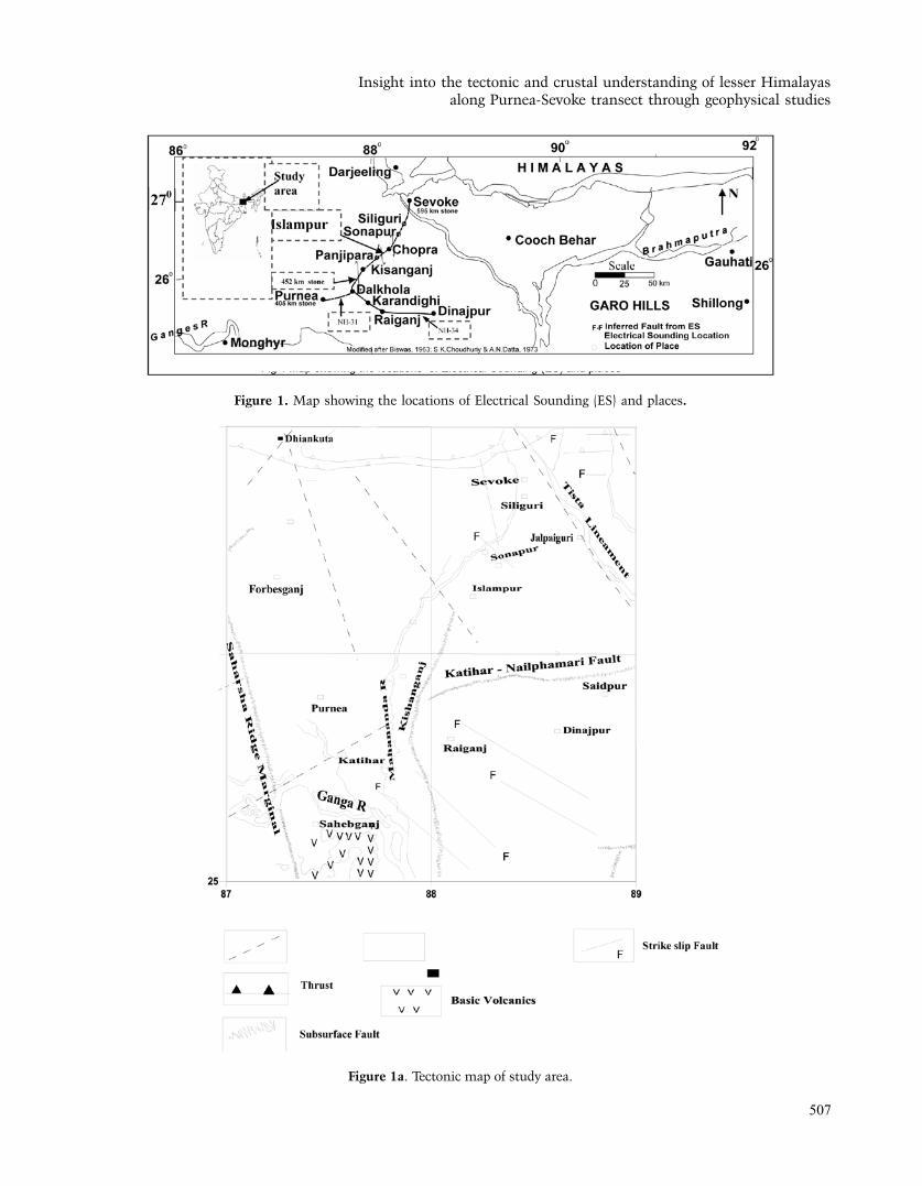
Insight into the tectonic and crustal understanding of lesser Himalayas along Purnea-sevoke transect through geophysical studies
507
Figure 1. Map showing the locations of electrical sounding (es) and places.
Figure 1a. tectonic map of study area.

D.C. naskar, L.K. Das and M.K. Rai
508
by the Geological survey of India in 1993 (Figure 1). It was expected that sediments settled in the basement depressions would be indicated by broad gravity “lows”. the magnetic method supplemented the gravity method in bringing out possible basement morphology. the deep resistivity soundings were taken at suitable locations to determine depths to the basement rock and to obtain character and thicknesses of the different formations overlying the basement.
the gravity survey was conducted employing sodin (Canada) make gravimeters with a reading accuracy of 0.01 mGal and the magnetic survey was conducted employing scintrex (Canada) make digital grade vertical force magnetometer having a reading accuracy of 1 to 10 nt. A scintrex 10 KVA time domain resistivity unit was used for field surveys. RDC-10 receiver of scintrex make was used for measuring the potential difference between the two non-polarisable electrodes (copper dipped in saturated copper sulphate solution).
Deep resistivity sounding
Resistivity of rocks is an important parameter for mapping crustal structures which may provide a clue on the processes of crustal evolution (Das et al., 1993). subsurface resistivity distribution is directly related to the physical character of the lithological units. Variation in resistivity of the rocks is the main source of electrical anomaly. Alpin et al., (1966) have used this technique for crustal mapping extensively in europe. Van Ziji (1977; 1978) effectively used this technique in south Africa. Blaine Webster (1997) successfully utilized this technique in Canada. In the present area of investigation, along the transect Purnea-sevoke, fourteen geoelectric soundings have been carried out (Figure 1) with R (separation between transmitting and receiving dipoles) as large as 8-10 km. the shallower part upto AB/2= 3 km was covered by using schlumberger electrode array to avoid the effects of lateral inhomogeneity. Azimuthal dipole sounding can be interpreted directly in terms of layer parameters by using two/multilayer master curves, when the azimuth angle is small (less than 10-15°). Inter-convertibility of dipole-apparent resistivities are discussed in Bhattacharyya and Patra (1968), Koefoed (1979). the resistivity sounding curves were initially interpreted using “orellana and Mooney” master curves (orellana and Mooney, 1966). A standard inverse modeling program ‘ResIst’ (Vander Velpen, 1988) has been used to get the layer parameters i.e. resistivity and thickness of different subsurface layers having distinct resistivity values. A four layer subsurface set up i.e. the Archaean basement overlain by the Gondwanas, the siwalik and the Quaternary alluvium is normally expected in this
area. Due to high conductivity of the Quaternary as well as the tertiary formations, the penetration has been poor in most of the cases.
Resistivity interpretation along transect Purnea-Sevoke
the interpreted geological subsurface layers are characterized by a distinct range in resistivity values (Figure 2 & 3). thus the very high order of resistivity varying from 1100-2400 ohm-m is interpreted as a boulder bed near the surface (es-10, 11, 12 & 14) around sonapur, Chopra, siliguri and sevoke. the lowest resistivity order is ranging from 10-39 ohm-m around Dalkhola, Purnea, Chopra and sonapur area varying in thickness from 2495-3150 m and appears at depths ranging from 922-2495 m, minimum at around Purnea and maximum at around Dalkhola. this is interpreted as the signature of siwaliks in the study area (es-1, 2, 3, 4, 5, 10 & 11). Presence of lateral inhomogeneities are observed around Kishanganj and Islampur areas which may be due to the presence of faulted subsurface structures (es-6, 7, 8).
A notable feature is observed in between siliguri and sevoke (es-14) where resistivity value of 1100 ohm-m near the surface persists with depth. However after 40 m depth this resistivity value suddenly falls. this is interpreted to be due to the presence of siwaliks at depth. the high resistivity basement is encountered at a depth varying from 2917-4450 m around Dalkhola and Kishanganj area (es-1 & 5). An onGC borehole, (500 m from es-2) towards Purnea, encountered siwaliks (around 2 km) followed by upper (369 m) and lower (1253 m) Gondwanas over the Archaean basement.
Apparent resistivity pseudo depth section along Purnea-Siliguri Highway :
An apparent resistivity pseudo-section along Purnea-siliguri Highway is shown in Figure 4. the section shows four distinct breaks (faults). these faults are located near km st 452, 493, 510 and north of km st 526 respectively. the relative displacements of the basement are shown by arrows depicted on the figure around the interpreted faults. of particular interest is the zone between km st 452 and 493 where resistivities to the tune of 1000-2000 ohm-m is mapped at comparatively shallower level. this is interpreted as the basement resistivity and the basement is up-arched (convex upwards) in this zone. this zone may be interesting for Gondwana sediments at shallower depth and/or oil and gas. In the rest of the area north of km st 493 the basement deepens further with another fault at km st 524.

Insight into the tectonic and crustal understanding of lesser Himalayas along Purnea-sevoke transect through geophysical studies
509
Figure 2. Dipole-dipole resistivity sounding es-1 to es-8 centered at respective km stone.
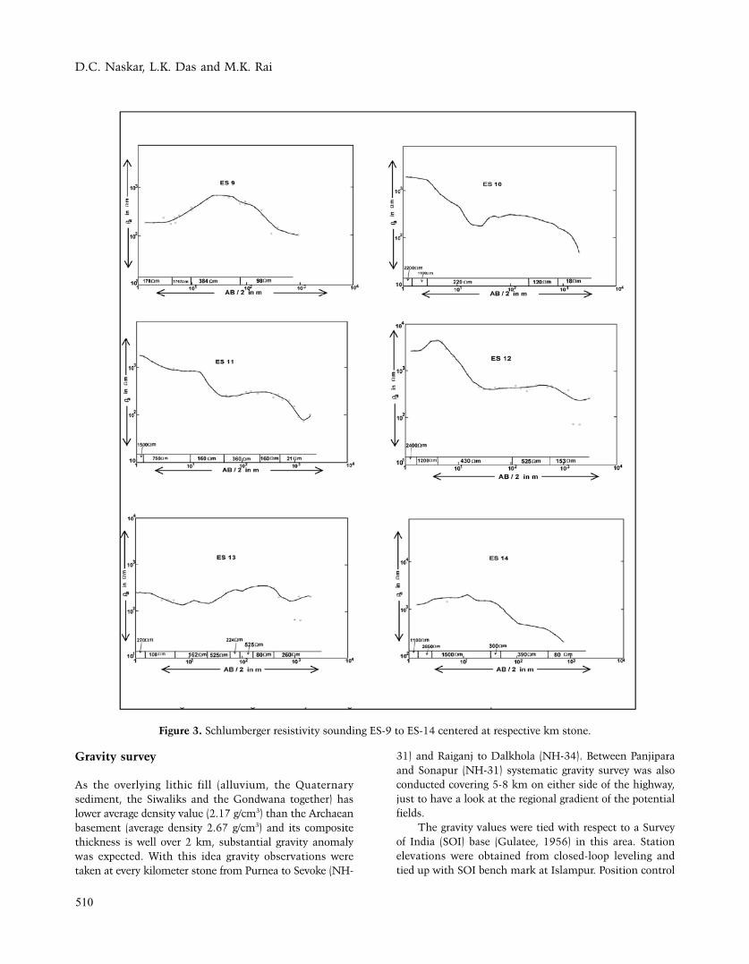
D.C. naskar, L.K. Das and M.K. Rai
510
Gravity survey
As the overlying lithic fill (alluvium, the Quaternary sediment, the siwaliks and the Gondwana together) has lower average density value (2.17 g/cm3) than the Archaean basement (average density 2.67 g/cm3) and its composite thickness is well over 2 km, substantial gravity anomaly was expected. With this idea gravity observations were taken at every kilometer stone from Purnea to sevoke (nH-
31) and Raiganj to Dalkhola (nH-34). Between Panjipara and sonapur (nH-31) systematic gravity survey was also conducted covering 5-8 km on either side of the highway, just to have a look at the regional gradient of the potential fields.
the gravity values were tied with respect to a survey of India (soI) base (Gulatee, 1956) in this area. station elevations were obtained from closed-loop leveling and tied up with soI bench mark at Islampur. Position control
Figure 3. schlumberger resistivity sounding es-9 to es-14 centered at respective km stone.
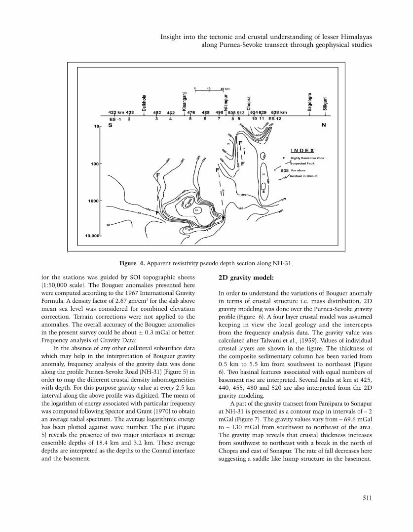
Insight into the tectonic and crustal understanding of lesser Himalayas along Purnea-sevoke transect through geophysical studies
511
for the stations was guided by soI topographic sheets (1:50,000 scale). the Bouguer anomalies presented here were computed according to the 1967 International Gravity Formula. A density factor of 2.67 gm/cm3 for the slab above mean sea level was considered for combined elevation correction. terrain corrections were not applied to the anomalies. the overall accuracy of the Bouguer anomalies in the present survey could be about ± 0.3 mGal or better. Frequency analysis of Gravity Data:
In the absence of any other collateral subsurface data which may help in the interpretation of Bouguer gravity anomaly, frequency analysis of the gravity data was done along the profile Purnea-sevoke Road (nH-31) (Figure 5) in order to map the different crustal density inhomogeneities with depth. For this purpose gravity value at every 2.5 km interval along the above profile was digitized. the mean of the logarithm of energy associated with particular frequency was computed following spector and Grant (1970) to obtain an average radial spectrum. the average logarithmic energy has been plotted against wave number. the plot (Figure 5) reveals the presence of two major interfaces at average ensemble depths of 18.4 km and 3.2 km. these average depths are interpreted as the depths to the Conrad interface and the basement.
2D gravity model:
In order to understand the variations of Bouguer anomaly in terms of crustal structure i.e. mass distribution, 2D gravity modeling was done over the Purnea-sevoke gravity profile (Figure 6). A four layer crustal model was assumed keeping in view the local geology and the intercepts from the frequency analysis data. the gravity value was calculated after talwani et al., (1959). Values of individual crustal layers are shown in the figure. the thickness of the composite sedimentary column has been varied from 0.5 km to 5.5 km from southwest to northeast (Figure 6). two basinal features associated with equal numbers of basement rise are interpreted. several faults at km st 425, 440, 455, 480 and 520 are also interpreted from the 2D gravity modeling.
A part of the gravity transect from Panjipara to sonapur at nH-31 is presented as a contour map in intervals of – 2 mGal (Figure 7). the gravity values vary from – 69.6 mGal to – 130 mGal from southwest to northeast of the area. the gravity map reveals that crustal thickness increases from southwest to northeast with a break in the north of Chopra and east of sonapur. the rate of fall decreases here suggesting a saddle like hump structure in the basement.
Figure 4. Apparent resistivity pseudo depth section along nH-31.

D.C. naskar, L.K. Das and M.K. Rai
512
A separate Bouguer anomaly profile along nH-34 between Raiganj and Dalkhola (Figure 8), shows a continuous fall of gravity anomaly at the rate of 1 mGal/km upto 425 km stone. After that a sharp fall in gravity value has been interpreted to be due to a basement fault
dipping towards north at 432 km stone. this is interpreted to be the signature of the buried Malda-Kishanganj fault (Figure 1a). thickening of crust towards north is probably due to sagging of the crustal block at the foot hill of Himalaya.
Figure 5. spectral analysis of the Bouguer anomaly profile from Purnea to sevoke along nH-31.
Figure 6. Bouguer anomaly profile and 2D gravity model from Purnea to sevoke along nH-31. σ = – 0.5 g/cc represent density contrast. P = 2.17 g/cc indicates density of the layer.
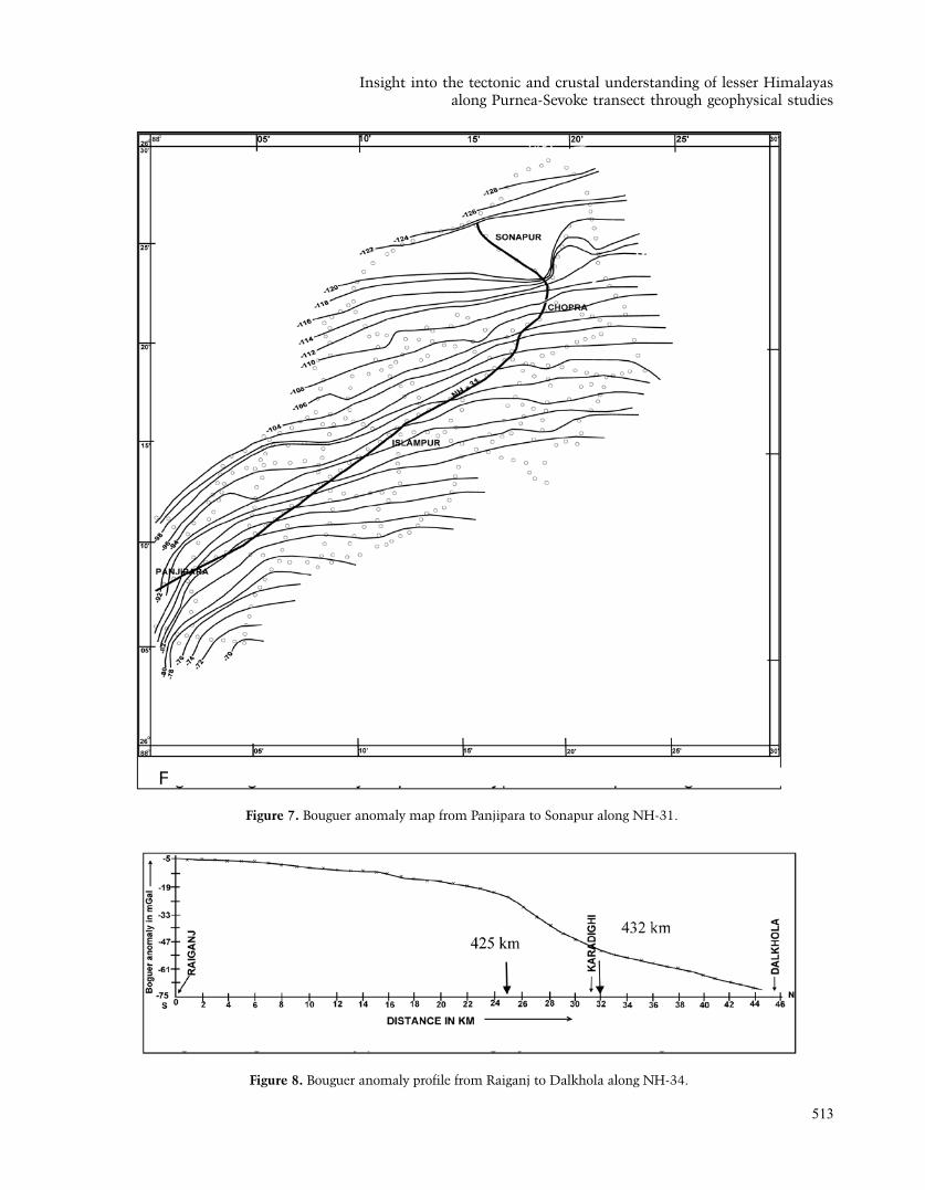
Insight into the tectonic and crustal understanding of lesser Himalayas along Purnea-sevoke transect through geophysical studies
513
Figure 7. Bouguer anomaly map from Panjipara to sonapur along nH-31.
Figure 8. Bouguer anomaly profile from Raiganj to Dalkhola along nH-34.
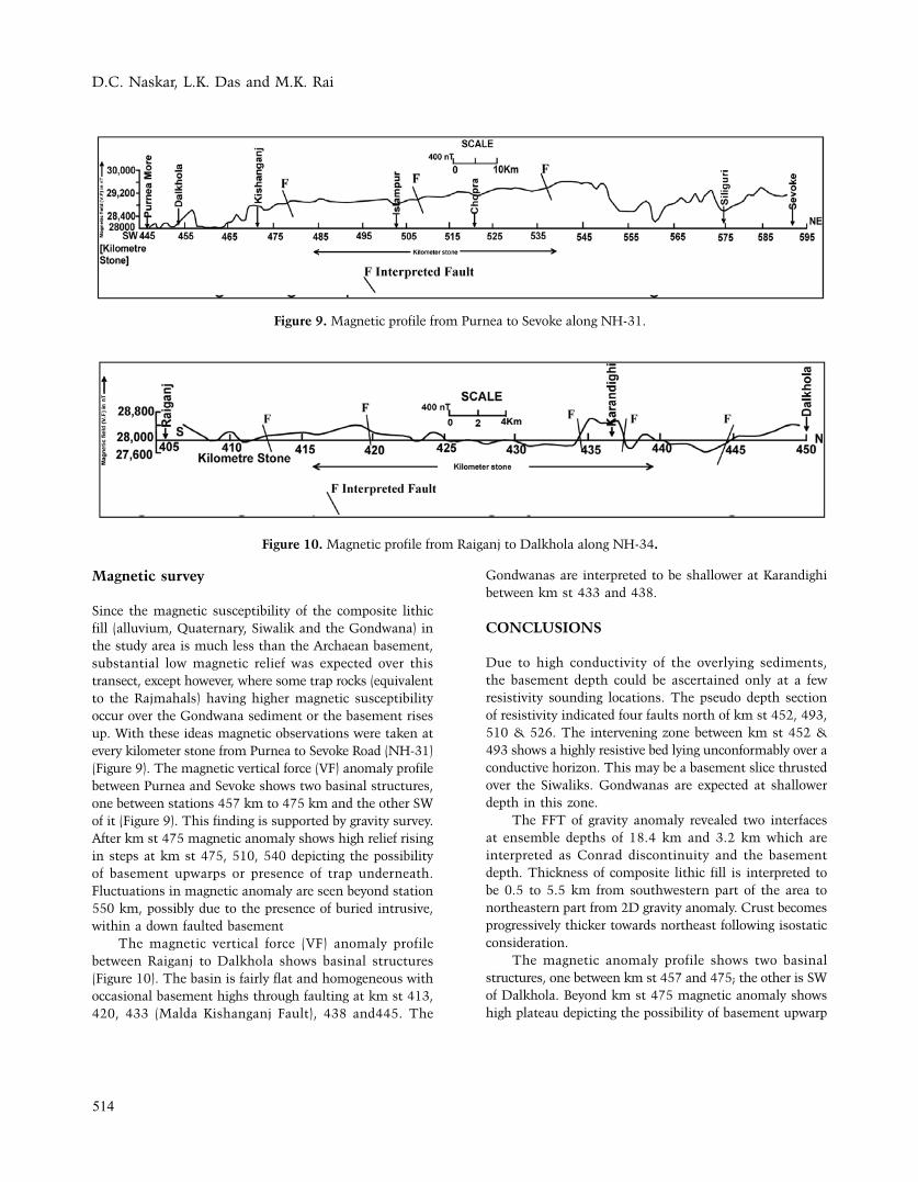
D.C. naskar, L.K. Das and M.K. Rai
514
Magnetic survey
since the magnetic susceptibility of the composite lithic fill (alluvium, Quaternary, siwalik and the Gondwana) in the study area is much less than the Archaean basement, substantial low magnetic relief was expected over this transect, except however, where some trap rocks (equivalent to the Rajmahals) having higher magnetic susceptibility occur over the Gondwana sediment or the basement rises up. With these ideas magnetic observations were taken at every kilometer stone from Purnea to sevoke Road (nH-31) (Figure 9). the magnetic vertical force (VF) anomaly profile between Purnea and sevoke shows two basinal structures, one between stations 457 km to 475 km and the other sW of it (Figure 9). this finding is supported by gravity survey. After km st 475 magnetic anomaly shows high relief rising in steps at km st 475, 510, 540 depicting the possibility of basement upwarps or presence of trap underneath. Fluctuations in magnetic anomaly are seen beyond station 550 km, possibly due to the presence of buried intrusive, within a down faulted basement
the magnetic vertical force (VF) anomaly profile between Raiganj to Dalkhola shows basinal structures (Figure 10). the basin is fairly flat and homogeneous with occasional basement highs through faulting at km st 413, 420, 433 (Malda Kishanganj Fault), 438 and445. the
Gondwanas are interpreted to be shallower at Karandighi between km st 433 and 438.
CONCLUSIONS
Due to high conductivity of the overlying sediments, the basement depth could be ascertained only at a few resistivity sounding locations. the pseudo depth section of resistivity indicated four faults north of km st 452, 493, 510 & 526. the intervening zone between km st 452 & 493 shows a highly resistive bed lying unconformably over a conductive horizon. this may be a basement slice thrusted over the siwaliks. Gondwanas are expected at shallower depth in this zone.
the FFt of gravity anomaly revealed two interfaces at ensemble depths of 18.4 km and 3.2 km which are interpreted as Conrad discontinuity and the basement depth. thickness of composite lithic fill is interpreted to be 0.5 to 5.5 km from southwestern part of the area to northeastern part from 2D gravity anomaly. Crust becomes progressively thicker towards northeast following isostatic consideration.
the magnetic anomaly profile shows two basinal structures, one between km st 457 and 475; the other is sW of Dalkhola. Beyond km st 475 magnetic anomaly shows high plateau depicting the possibility of basement upwarp
Figure 9. Magnetic profile from Purnea to sevoke along nH-31.
Figure 10. Magnetic profile from Raiganj to Dalkhola along nH-34.

Insight into the tectonic and crustal understanding of lesser Himalayas along Purnea-sevoke transect through geophysical studies
515
in steps and/or trap underneath. Fluctuations in magnetic anomaly are seen beyond station 550 km possibly due to the presence of intrusive, in a downthrown basement.
ACKNOWLEDGEMENTS
the Director General, Geological survey of India is gratefully acknowledged for his kind permission to publish the paper. Authors are grateful to Prof.B.V.s.Murthy for constructive review and editing and the Chief editor for his encouragement.
Compliance with Ethical Standards
the authors declare that they have no conflict of interest and adhere to copyright norms.
REFERENCES
Alpin, L.M., Berdichevskii, M.n., Vendrintsev, G.A., and
Zagarmister, A.M., 1966. Dipole methods for measuring
earth conductivity. translated by G.V. Keller. A special
research report, C.B. new York.
Bhattacharya, A.R., 2008. Basement rocks of the Kumaun-Garhwal
Himalaya: some implications for the Himalayan tectonics.
earth sci. India, v.1, no.1, pp: 1-11.
Bhattacharya, P.K., and Patra, H.P., 1968. Direct current geoelectric
sounding: Principles and interpretation. elsevier Publishing
Company, Amsterdam.
Biswas, B., 1963. Results of explorationfor petroleum in the
western part of the Bengal basin, India.Proc. 2 nd. symp.
Developments in Petroleum Research. eCAFe Miner. Res.
Dev. ser., v.18, part 1, pp: 241-250.
Blaine Webster, 1997. Logistical and interpretative report on
spectral IP/resistivity survey conducted on Harker/Holloway
townships, northeastern ontario for Franco nevada Mining
Corporation. JVX Ltd. Geoscience Assessment office, JVX
Ref: 9762, Canada.
Choudhury, s.K., and Dutta, A.n., 1973. Bouguer gravity and its
geologic evaluation in the western part of the Bengal basin
and adjoining area, India. Residual gravity in theory and
practice. Geophysics, v.14, pp: 39-56.
Das, L.K., Rai, M.K., naskar, D.C., and saxena, A.s., 1993. A
report on the integrated geophysical survey along Purnea-
Gangtok transect. GsI Unpub. Rep.
Dst, expert Group, 1995. Report of the expert group on the nW
Himalayan geotransect programme (nWHGP), earth system
science division, Department of science and technology,
Govt. of India, Unpub. Report.
Gulatee, B.L., 1956. Gravity data in India. surv. India. techn.
Pap., v.10, pp: 106.
Koefoed, o., 1979. Geosounding Principles-I, resistivity sounding
measurements. elsevier scientific Publishing Company,
Amsterdam.
orellana, e., and Mooney, H.M., 1966. Water table and curves
for vertical electrical sounding over layered structures.
Interetencia, Madrid, spain.
Reddy, C.D., and Arora, B.R., 1993. Quantitative interpretation
of geomagnetic induction response across the thrust zones
of Himalaya along the Ganga -Yamuna valley, J. Geomag.
Geoelectr., v.45, pp: 775-785.
sengupta, s., 1966. Geological and geophysical studies in the
western part of Bengal basin. Int. Bull. Am. Assoc. Pet.
Geol., v.50, no.5, pp: 1001-1017.
spector, A., and Grant, F.s., 1970. statistical method for interpreting
aeromagnetic data. Geophysics, v.35, pp: 293-302.
talwani, M., Worzel, J.L. and Landisman, M., 1959. Rapid gravity
computations for two dimensional bodies, the mid-oceanic
submarine fracture zone. Jour. Geophy. Res., v.64, no.1,
pp: 49-59.
Vander Velpen, B.P.A., 1988. A computer processing package for
DC resistivity interpretation for an IBM compatibles. ItC,
Jour. 4, the netherlands.
Van Ziji, J.s.V., 1977. electrical studies of the deep crust in
various provinces of south Africa. In: the earth’s crust, J.
Headcock (ed.), Geophys. Monogr. Am. Geophys. Unions,
v.20, pp: 470-500.
Van Ziji, 1978. the relationship between the deep electrical
resistivity structure and tectonic provinces in south Africa.
trans. Geol. soc. Afr., v.81, pp: 129-142.
Yin, An., 2006. Cenozoic tectonic evolution of the Himalayan
orogen as constrained by along-strike variation of structural
geometry, exhumation history, and foreland sedimentation.
earth sci. Reviews, v.76, pp: 1-131.

P.R.Reddy
516
-AN OPINION
Is Micro irrigation viable in helping small and marginal farmers? -need for an in depth scientific study
P.R.ReddyDirector Grade scientist ( Retd ), CsIR-nGRI, Hyderabad, 500 007.
email: [email protected]
AbSTRACTMicro irrigation is considered the best irrigation technique, especially in water stressed arid and semi arid tracts. However, there are some impediments to make it a viable irrigation practice, due to some practical problems encountered by economically backward small and marginal farmers. In this write up an effort has been made to analyse various facets of micro irrigation.
PREAMbLE:
It is well established that per hectare yield in many parts of our country is abysmally low compared to developed countries and our farming community, comprising mostly small and marginal farmers, in general are struggling to overcome various hurdles, including insufficient water availability. When we look in to phenomenal strides made by Israel in producing different types of crops in arid tracts that have very limited water availability, we naturally feel that the existing belief that insufficient availability of water is the basic cause for farmers` plight may need a relook. the significant strides made by Israel have been achieved through implementation of micro irrigation practices. However, as Israel and India have different socio-economic structures and varied priorities, it is essential to take stock of various factors before arriving at any conclusion.
Irrespective of claims and counter claims, our backwardness, according to experts is mainly due to our adapting age old irrigation and farming practices that lead to not only wastage of water but also production of inferior variety of final produce, both in quality and quantity. While such an opinion is to a major extent true, one wonders why our scientific and technical experts are unable to solve the existing dismal scenario, especially in semiarid and arid tracts of our country. Having witnessed the plight of small, marginal and even middle class farmers and death of thousands of farmers every year in many states I have tried to understand basic reasons, apart from socio-economic, for these setbacks. While it is not prudent to say that this small exercise might provide answers to the vexed problem, where many experts faced hurdles at every stage of their studies, I have decided to present some details that could be used by committed experts in segregating the truth from false projections. I feel such a relook is essential as many new initiatives are being planned by the present government to strengthen our production capabilities in all the sectors, including agriculture.
Need for Suggested scientific study:
After going through some excellent reports and publications, I came to the conclusion that our scientific exercises in spite of producing valuable results are not translated properly as viable execution practices, due to various reasons including non-implementation of umpteen number of recommendations. the suggested study should first make use of wealth of valuable data already available in the form of technical reports and scientific publications. once this is done and useful information is gathered it is essential to divide our water stressed semiarid and arid tracts in to sub divisions based on topography, average rainfall, and effective cropping pattern. Within semiarid tracts due to recent monsoon aberrations some segments that fall under rain shadow zones have become much worse with soil erosion and increased weather related aberrations. since recent el nino effect has adversely affected many parts of our country especially telangana, Vidarbha and Rayalaseema apart from parts of Karnataka and Rajasthan it may be better to select two districts each from these states/ sub states for area specific pilot plant studies. since our agriculture sector (as many others) is controlled by industrialists, business magnates, powerful administrators and influential politicians, all of whom do not give due importance to our scientific pursuits assuming our scientists are not capable enough of producing solutions to our problems even good studies and resultant useful results are not taken in to cognizance before preparing project reports and scheduling various time bound and area specific norms. Unfortunately, many learned members of our scientific community add fuel to the fire by stating our scientific pursuits are indeed mediocre, brushing aside all the studies (good and bad) as irrelevant, a way of receiving attention and focusing on their own superiority. those who really want welfare of our masses always silently provide needed advises that are implementable at the field level.
J. Ind. Geophys. Union ( september 2016 )v.20, no.5, pp: 516-519
Is Micro irrigation viable in helping small and marginal farmers?-need for an in depth scientific study.
517
In such a scenario our experts find it difficult to effectively take up pilot projects to wean off our farming community from age old irrigation practices. I say so as I am unable to understand why specific recommendations, made after micro irrigation studies, that have clearly shown the efficacy of micro irrigation technology are not put into practice on large scale as viable agriculture practices.
out of many outstanding reports I am impressed by the excellent inputs provided by Vaibhav Bhamoriya and susan Mathew in their technical report entitled “An Analysis of Resource Conservation technology: A Case of Micro-Irrigation system (Drip Irrigation)” released in 2014. I am pained to say the details given in this report and couple of other reports on minor irrigation studies in Karnataka and sri Lanka have not been properly made use of in propagating importance of Micro irrigation. the subject of the report by Vaibhav and susan is very important in context of agricultural development and resource use efficiency. However, as the analysis is rated as qualitative in nature, relying on subjective judgments rather than quantitative measurements by the expert who reviewed it, my suggested study assumes greater importance and relevance. the suggested study, however, should make use of some excellent details given in the report cited above before fixing up specific objectives to make the study more useful and adaptable.
Proposed initiative:
Data shows that micro irrigation such as drip systems can reduce water losses and increase crop production -- if it overcomes some hurdles. It is well known that the limitation of this method is its high initial cost, which is beyond purchasing capacity of small and marginal farmers, that’s why it is normally adopted by large land holdings farmers. As a policy to encourage the use of such system, the Ministry of Agriculture, Government of India, provides subsidy to the tune of 50% to small and marginal farmers under national Mission on Micro Irrigation. However, these subsidies benefit more the industrialists/ manufacturers of drip/ sprinkler irrigation gadgets than the small farmer. this set back can be overcome, if government ensures proper installation and maintenance in addition to easy availability of running costs. Introduction of solar panels to lift water from ground level to overhead tank will enthuse small farmers living at remote places. success rate of its acceptance by small farmers depends on efficient interaction between extension workers and farmers.
Believing in micro irrigation importance, accepting recommendation of experts, Karnataka is planning the world's biggest micro irrigation project by bringing 7 lakh hectares of land under drip and other systems, and along with Maharashtra, is making drip irrigation mandatory for sugarcane cultivation. this didn't happen by accident;
rather the unsustainability of conventional irrigation practices has forced policy makers to pay greater attention to micro-irrigation practices, which primarily involve the use of sprinkler and drip irrigation. these systems supply water efficiently and reduce loss due to seepage, run off and evaporation. While a sprinkler would spray water uniformly over the field, drip irrigation systems supply water in drops to the root area of the plant.
there has been a constant rise in area under micro irrigation in India. However, despite their increasing popularity thanks to huge government subsidies, micro-irrigation techniques still serve only 5.71 per cent of the total irrigated area in the country. (Source:http://www.indiawaterportal.org/articles/micro-approach-thats-big-enough-fight-growing-water-crisis)
While appreciating the bold initiative of Karnataka, to make micro irrigation an important irrigation component in different semi-arid tracts of our country I have decided to project some salient points included in the report of Bhamoriya and Mathew. some of my own observations are also included, hoping the write up would be useful in taking stock of existing scenario and recommended initiatives to make Karnataka type projects to emerge in other states. since none of us who want healthy growth of our agriculture sector likes to see the usual impediments/ hurdles to such welfare measures I solicit support of our scientist brethren to come out with more specific/ focused presentations to strengthen the movement.
Drip Irrigation is viewed as a promising technology for its ability to support farmers in raising incomes and reducing poverty. A number of benefits have been ascribed to the use of micro-irrigation. In addition to saving of water these include increased yield and productivity of certain crops (especially spaced crops), labour cost savings, electricity savings, lesser pumping hours and hence easier irrigation, better crop growth and also better soil health. strong evidence exists claiming economic benefits from the adoption of micro-irrigation. However there exists little or sparse evidence of socio-economic benefits from the adoption of micro-irrigation. there are mentions of positive nutritional impact on adopting households as well but these are few and far apart. In spite of these advantages, the spread of micro – irrigation has been restricted to only a few pockets across India. the government has launched various schemes to promote micro – irrigation in the country. It set up the national Committee on use of Plastics in Agriculture (nCPA) which took up various schemes for the promotion of use of plastics, and in particular micro – irrigation systems. In agriculture, nABARD has been financing micro – irrigation systems since 1985. Maharashtra was the first state to introduce subsidies in 1986 – 87. subsidies ever since have been a regular and dominant phenomenon in the efforts to spread the use of drip irrigation. there is a new debate concerning

P.R.Reddy
518
the impact of micro-irrigation systems at various levels of water use for consideration of “water-saving” and also on the status of the resource (water resource) itself from the basin perspective. While these positives enthuse technical experts, negatives pose a problem as majority of our land holders have 1 to 10 acre holdings and introduction of these systems, on individual basis, in to small holdings is fraught with many setbacks. they according to me are; 1) lack of enthusiasm and motivation in part of small land holders in erecting and maintaining mechanised systems, when they are struggling to earn sufficiently to eke out a living; 2) absence of assured water source that ensures availability of water (even the limited); 3) dependence on outside expertise that needs running expenses; 4) non usability of the systems in producing staple food-rice/ wheat.
In addition to this negative mind set and practical problems some experts opine that “water-saving” is notional. they point out that while a farmer may save water for growing a given crop on a given plot in a given season however it may not necessarily result in water savings even at the farm level as the farmer is likely to use the “saved” water in a nearby plot to grow another crop. As a result there might be increase in crop output but no net water saving may result. there may also be a case wherein a farmer may save water on his farm but other famers draw out and use water from the aquifer resulting in no savings. some researchers and practitioners therefore believe that the commercialization of agriculture and increasing area under irrigation and / or intensifying agriculture with the aid of micro-irrigation might lead to unsustainability of agriculture in the long run enabling use of even the marginal water quantities and sources rather than their conservation. such complicated issues are resulting in a debate on the impact of micro-irrigation on agriculture and water resources. Understanding the impact of adoption of micro-irrigation is crucial for different states of India like Gujarat, Andhra Pradesh, telangana, Karnataka and Rajasthan giving a massive push to promote micro irrigation for water resource conservation is essential. the erstwhile Andhra Pradesh Micro-Irrigation Project (APMIP) claims to have brought 1.66 lakh ha. area under micro-irrigation during 2.5 years. At the same time there are pockets like Jalgaon and nashik in Maharashtra, narsinghpur and Maikaal in Madhya Pradesh where the market forces are leading to high adoption rates. In some pockets high adoption rates are observed even in the absence of government subsidies.
there is a need to understand the impact of micro-irrigation technology vis-a-vis resource conservation and other claimed benefits, before present status of Drip Irrigation Adoption is implemented. such a development is possible only if our committed scientific and technical community comes forward to lead the movement.
Micro-irrigation technologies are supported largely for one or more of the following profits: means of saving water in irrigated agriculture and averting the impending water crises, as a strategy to increase income and reduce poverty among the rural poor; to enhance the food and nutritional security of rural households; and as means to extend the limited available water over a large cropped area. the financial paybacks have been proved in many studies. Puran et al., (2010) have reported that the incremental increase in irrigated areas was about three-fold and the decline in labour use per hectare was by 78%. Also the economic returns to farmers` investments in micro-irrigation technologies are substantial. Financial resources and crop suitability are the stimulus for adoption of drip irrigation. though a key argument is that membership in a high caste group, poverty index and share of income from off-farm and non-farm activities, have a significant effect on the decision regarding the adoption of micro-irrigation technology (Mamara et al., 2005). Under these situations, it is highly required to analyse the issues, facts and constraints that are hindering the adoption and spread of micro-irrigation in different states, which will give appropriate signals for the expansion of the Micro-irrigation in the country, wherein researchers, extension workers and policy makers could play a key role (Palanisami et al., 2011).
Needed precautions in introducing time bound mega micro irrigation projects
since any mega irrigation projects, while implementing within a stipulated time, could lead to some setbacks Karnataka and Maharashtra initiatives of taking up micro irrigation in lakhs of hectares need some execution strategies. the following precautions are essential to ensure high percentage of success.
1. Area specific geomorphic aspects need to be taken in to cognizance in selecting and erecting drip irrigation components. the standard practice of incorporating a uniform design should be avoided.
2. soil structure, texture and composition in an agro-met unit needs to be taken in to consideration in selecting drip irrigation design including height, location and volume of overhead tank and design of distribution channels and velocity and droplet dimensions. In addition the type and quality of drip irrigation components needs to be given due importance. surface and subsurface water input availability, mode of pumping from input storage facility to overhead tank need to be evaluated in advance taking in to consideration frequency and magnitude of extreme weather events in the region, using past statistics.
3. Data pertaining to area specific evapotranspiration variations- wind velocity/ moisture content

Is Micro irrigation viable in helping small and marginal farmers?-need for an in depth scientific study.
519
should be given due importance, to make on spot variations in the design
4. Cropping pattern has to be decided depending on various aspects, including socio-economic factors, availability of quality seeds/ seedlings, frequent technical advisories including midcourse corrections to circumvent natural hazard related setbacks, final product storage and marketability.
5. Assured maintenance through trained personnel is vital for success of the project.
REFERENCES
Vaibhav Bhamoriya and susan Mathew, 2014. An Analysis of
Resource Conservation technology: A Case of Micro-
Irrigation system (Drip Irrigation), A technical Report of
Centre for Management in Agriculture, Indian Institute of
Management, Ahmedabad, pp:1-169.
Mamara, Regassa, e., Upadhyay, Bhawana and nagar, R.
K., 2005. Adoption and Impacts of Microirrigation
technologies: empirical Results from selected Localities of
Maharashtra and Gujarat states of India. Research Report
93, International Water Management Institute, sri Lanka.
Palanisami, K., Mohan, K., Kakumanu, K. R., Raman, s., 2011.
spread and economics of Micro-irrigation in India: evidence
from nine states. economic and Political Weekly, v.46 –
nos. 26 and 27.
Puran Mal, Malik, Dharmapal and Luhach, M. s., 2010. economic
analysis of tubewell driven sprinkler irrigation and furrow
irrigation for Agriculture in Haryana, India. In: World
Food systems – A contribution from europe, tropentag,
september 14-16, 2010 in Zurich.

520
I.C. Madhusudan
Reminiscences of a Field Geophysicist of Geological Survey of India
I.C. MadhusudanDirector Geophysics, selection grade (Retd, GsI)
After graduating in Applied Geophysics from Indian school of Mines Dhanbad in the year 1963, I joined GsI in a career spanning nearly 38 years. During this long tenure I was engaged in a wide range of investigations comprising predominantly of search for economic ore deposits
and secondarily of shallow seismic refraction surveys to locate suitable sites for steel plants, power supply stations, rail bridges and sea ports. there were also brief excursions into marine geophysics and oil exploration in my initial years. Marine activities off east and west coasts involved systematic measurement of variations in the earth’s magnetic field along specified traverses with concurrent determinations of ocean depth. I was also temporarily attached to a crew of the onGC conducting deep seismic reflection survey for oil in the Indo-Gangetic plains.
My expertise, however, has been almost entirely in the field of Mineral exploration or ‘Mining Geophysics’, as it is sometimes called, employing the entire range of electrical methods besides eM and magnetics. these projects were spread across Rajasthan, Gujarat, undivided Bihar, odissa and West Bengal. I intend to share here some of my experiences in ore search in the belief that they would be of some interest to younger geophysicists.
What was once regarded as the Hesatu-Belbathan polymetallic belt in Bihar (Jharkhand) is a notable example of belied hopes. Geological exploration complemented by drilling had gone on for as long as thirty five years. Much money and resources had been expended without producing any significant ore finds. At that stage I took the initiative to suggest a gravity survey to locate a magmatic chamber, if any, at depth whose plumes could then satisfactorily account for the mineral shows that are noticed commonly in the area. the survey did indeed bring out significant residual gravity anomalies bearing remarkable correlation to the surface mineral shows. this correlation bears indirect evidence of a magmatic chamber at depth whose plumes must have been the carriers of mineral bearing fluids. test drilling was accordingly suggested to confirm the surmised magmatic body but it does not seem to have been implemented so far.
the role of the magnetic method is often underrated in base metal exploration whereas it can be the only
savior available to detect sulphide bodies either directly or indirectly in certain geological milieus. sindesharkalan and Khetri in southern and northern Rajasthan, the singhbhum copper belt in Jharkhand and Gorubathan area in Darjeeling of north Bengal may be cited as typical examples:
sindesharkalan in Udaipur district was investigated for over three years by eM, sP, IP and Magnetics. While eM and sP were quite effective in tracing the graphitic horizon hosting sulphides, they were of little help in locating sulphide ore bodies as such. the magnetic picture on the other hand showed low order anomalies distinctly superimposed over a relatively flat background. When drilled these low intensity anomalies were found to correlate with basemetal sulphides carrying pyrrhotite in good measure. this finding went a long way in optimizing further exploration strategies and substantially reducing the cost of exploration.In the Khetri copper belt again drilling of low intensity magnetic anomalies across extensive sand cover have proved copper sulphides with associated pyrrhotite.
In Kharkhola area of Gorubathan rich zinc and lead sulphide ores with associated gold and silver are hosted by a huge magnetite quartzite formation most of which is buried under debris brought down from the upper reaches of the Himalayas. the geophysical problem was essentially to map the concealed extensions under cover of this host formation. this was successfully accomplished by a simple magnetic survey. the resulting geophysical map of the host rock not only explained why some of the boreholes drilled earlier had turned out to be barren of ore but also served the far more important purpose of effectively guiding future drilling operations.
Like the magnetic method, sP too has by and large taken a back seat in basemetal exploration following the emergence of more modern eM and IP techniques. And yet, given favourable conditions, sP can provide clinching evidence of the presence or otherwise of an ore body when indications from other methods turn out to be ambiguous or uncertain. sP has also been remarkably successful in locating graphite bodies. I had the opportunity also of conducting borehole sP measurements that successfully lead to location of targets missed in earlier exploratory drilling. In estimating depths to the source from sP profiles, thumb rules in my experience have worked better than rigorous modeling. such thumb rules enabled the preparation of the depth section of a graphite body in
J. Ind. Geophys. Union ( september 2016 )v.20, no.5, pp: 520-521

521
Reminiscences of a Field Geophysicist of Geological survey of India
sambalpur district, which matched remarkably well with the actual depth section prepared by the company mining the property.
As disseminated sulphide ores are more the rule than exception, IP has found extensive application particularly in this country. I had the opportunity to carry out IP surveys in Agucha area of Bhilwara district, Rajasthan. Agucha is quite well known for its rich zinc-lead ores with associated silver and minor amounts of iron and copper sulphides. the host rock here is graphitic schist within Banded gneissic complex. the conductive graphitic schist disseminated abundantly with resistive sphalerite offers itself as a good IP target. time domain IP surveys were carried out over the years 1980-’83 with a three electrode array. the deposit has a well defined sW limit with a clear plunge towards ne. one of the boreholes in the ne gave evidences of possible pinching of the load in a shallow intersection. this drilling evidence was quite misleading as it could have meant termination of mining activity beyond this point. Geophysics saved the day so to say. IP traverses brought out strong chargeability anomalies that persisted with increasing array length actually suggesting
richer lodes at depth in the northeast. this is a clear case of geophysics effectively guiding mining operations. It is heartening to learn deep reflection profiling studies by nGRI revealed presence of potential ore deposits extending to deeper horizons.
the few instances recounted here are intended to give some idea of the significant role geophysics has played in effectuating exploration in some of the well known mineral belts in the country. While this ought to be a matter of legitimate pride to any geophysicist, it must also be admitted that borehole geophysics has yet not come into its own in this country. this is an unfortunate lacuna that needs to be filled essentially by the exploiting agencies to guide their day to day drilling and mining activity. needless to mention that systematic application of multi-method borehole geophysics would make a big difference to efficiency and economy of both exploration and mining.
As I look back over my cherished years in GsI, I am filled with a deep sense of fulfillment, fulfillment perhaps not so much in terms of discoveries made as in terms of having given all of myself and the very best of myself to the task on hand day after day and year after year!
o o o o o o o o o o o o o o o o o o o o o o o o o o o o o o o o o o o o o o o o o o o o o o o o o o o o o o o o
New Director for CSIR-NGRI
Dr. V.M. Tiwari, former Scientist of CSIR-NGRI and also former Director of National Centre for Earth System Studies, Tiruvananthapuram took charge as Director of CSIR-NGRI, Hyderabad on 11th July, 2016.
Editorial Board of JIGU wishes him successful tenure as Director of CSIR-NGRI and solicits his support to JIGU.
o o o o o o o o o o o o o o o o o o o o o o o o o o o o o o o o o o o o o o o o o o o o o o o o o o o o o o o o

523
the Journal of Indian Geophysical Union (J-IGU), published bimonthly by the Indian Geophysical Union (IGU), is an interdisciplinary journal from India that publishes high-quality research in earth sciences with special emphasis on the topics pertaining to the Indian subcontinent and the surrounding Indian ocean region. the journal covers several disciplines of earth sciences such as the Geosphere, its watery and gaseous envelopes (the Hydrosphere, the Cryosphere and the Atmosphere), and life (the Biosphere). It also publishes articles on space and Planetary sciences. J-IGU welcomes contributions under the following categories:
• Research papers reporting development of new theoretical methods, new techniques of data processing, development of area specific models, new experimental findings and results.
• Review articles providing comprehensive overview of a significant research field related to earth system sciences
In addition, J-IGU also welcomes short communications on opinion and report on scientific activity, personal information, book reviews and news and views.
the manuscript should be submitted electronically as a single pdf file including the main text, figures, tables, and any other supplementary information along with the signed "Declaration Letter". the manuscript should be submitted by email (([email protected]) to the Chief editor.
After acceptance of the manuscript the corresponding author would be required to submit all source files (text and tables in word format) and figures in high resolution standard (*.jpg, *.tiff, *.bmp) format. these files may be submitted to the editor as a single *.zip file along with the "Copyright transfer statement".
IMPORTANT INFORMATION
Ethics in publishingJ-IGU is committed to ensuring ethics in publication and takes a serious view of plagiarism including self-plagiarism in manuscripts submitted to the journal. Authors are advised to ensure ethical values by submitting only their original work and due acknowledgement to the work of others in case used in the manuscript. Authors must also refrain from submitting the same manuscript to more than one journal concurrently or publish the same piece of research work in more than one journal, which is unethical and unacceptable. Chief editor of J-IGU is committed to make every reasonable effort to investigate any allegations of plagiarism brought to his attention, as well as instances that come up during the peer review process and has full authority to retract any plagiarized publication from the journal and take appropriate action against such authors if it is proven that such a misconduct was intentional.
similarly, Chief editor, Associate editors, editorial board members and Reviewers are also expected to follow ethical norms of publishing by ensuring that they don’t use any unpublished information, communicated to them for editorial or review purpose, in their own research without the explicit written consent of the author. they are also expected to keep manuscript/ data/ observations/ any other information related to the peer review confidential to protect the interest of the authors. Reviewers should refrain from reviewing the manuscripts in which they have conflicts of interest resulting from competitive, collaborative, or other relationships or connections with any of the authors, companies, or institutions connected to the manuscript.
Conflict of interestAll authors are requested to disclose any actual or potential conflict of interest including any financial, personal or other relationships with other people or organizations within three years of beginning the submitted work that could inappropriately influence, or be perceived to influence, their work.
Submission declaration submission of a manuscript implies that the work has not been published previously and it is not under consideration for publication elsewhere, and that if accepted it will not be published elsewhere in the same or any other form, in english or in any other language, without the written consent of the publisher. It also implies that the authors have taken necessary approval from the competent authority of the institute/organization where the work was carried out.
CopyrightAfter acceptance of the manuscript the corresponding author would be required to sign and submit the "Copyright transfer statement".
MANUSCRIPT PREPARATION
the corresponding author should be identified (include e-mail address, Phone/Mobile number). Full affiliation and postal address must be given for all co-authors.
Abstract:An abstract of not more than 300 words must be included.
Text:the manuscript should be structured to include a front page containing the title, Author(s) name, affiliation and address of the institute where the work was carried out, a short title, and 5-to-6 index terms/Key words. Author(s) present address, if different from the above mentioned address,
GUIDELINES TO AUTHORS
may be given in the footnote. the corresponding author should be identified with an asterisk and his/her email ID should be provided. this page should be followed by the main text consisting of Abstract, Introduction, Methods/ techniques/ Area description, Results, Discussion, Conclusions, Acknowledgements, and References. tables and Figures with captions should be inserted in the main text of the manuscript at appropriate places. text should be 1.5 spacing with 12 pt font; lines should be numbered.
Figures/ Illustrations:All figures should be provided in camera-ready form, suitable for reproduction (which may include reduction) without retouching. Figures in high-resolution (at least 300 dpi) standard formats (*.jpg, *.tiff, *.bmp) are acceptable. Figures should be numbered according to their sequence in the text. References should be made in the text to each figure. each figure should have a suitable caption.
Tables:Authors should take note of the limitations set by the size and layout of the journal. table should not exceed the printed area of the page. they should be typed on separate sheets and details about the tables should be given in the text. Heading should be brief. Large tables should be avoided and may be provided as supplementary information, if required.
Equations:equations should be numbered sequentially with Arabic numerals and cited in the text. subscripts and superscripts should be set off clearly. equation writing software that presents each equation as an object in Ms Word will be accepted. style and convention adopted for the equations should be uniform throughout the paper.
References:All references to publications cited in the main text should be presented as a list of references following the text and all references in the list must be cited in the text. References should be arranged chronologically, in the text. the list of references should be arranged alphabetically at the end of the paper.
References should be given in the following form:Kaila, K.L., Reddy, P.R., Mall, D.M., Venkateswarlu, n., Krishna, V.G., and Prasad, A.s.s.s.R.s., 1992. Crustal structure of the west Bengal Basin from deep seismic sounding investigations, Geophys. J. Int., v.111, no., pp: 45-66.
REVIEW PROCESS:
All manuscripts submitted to the journal are peer-reviewed. It is advisable to send the contact details of 4 potential reviewers along with the manuscript to expedite the review process. Chief editor has the option to select reviewers from the list or choose different reviewers. the review process usually takes about 3 months. All enquiries regarding the manuscript may be addressed to the Chief editor. It is helpful to have the list of several potential reviewers covering various research topics/themes/ sub themes, to avoid delay in choosing the right persons. Authors and learned experts may help in developing a reference manual, which could be updated from time to time.
GALLEy PROOF:
technical editing of manuscripts is performed by the editorial board. the author is asked to check the galley proof for typographical errors and to answer queries from the Chief editor. Authors are requested to return the corrected proof within two days of its receipt to ensure uninterrupted processing. the Chief editor will not accept new material in proof unless permission from the editorial board has been obtained for the addition of a “note added in proof”. Authors are liable for the cost of excessive alterations to galley proof.
PUbLICATION CHARGES:
there are no page charges for publication and printing charges for b/w figures, provided length of printed manuscript is not more than 10 pages. For every additional page Rs.3000/ is charged, basically to meet publication costs. Also, in view of substantial cost involved in printing of color figures, author will be charged for printing of pages containing color figures @ Rs.2,500/- per page. the charges may be revised at any time based on cost of printing and production. Author will receive an estimate/ invoice of the additional page charges, color figures reproduction cost along with the galley proof. It is the responsibility of the author to remit the additional page charges and/ or color figures reproduction cost within one month of the receipt of the estimate/invoice.
the corresponding author will receive a soft copy (pdf format) of his/her published article. should the author desire to purchase reprints of his/her publication, he/she must send the duly signed Reprint order Form (accompanies the galley proof and contains price details) along with the corrected galley proof to the Chief editor. the reprint charges must be paid within one month of sending the Reprint order Form.
Any payment related to additional page charges, printing of color figures and/or purchase of reprints should be made in the form of a Demand Draft in the name of Treasurer, Indian Geophysical Union, payable at Hyderabad.
You may download the pdf file from: http://www.j-igu.in/IGU-Guide-forAuthors.pdf