An online railway traffic prediction model

Pavle Kecman, Rob M.P. GoverdeDelft University of Technology, Department of Transport and Planning

Stevinweg 1, 2628 CN Delft, The Netherlandse-mail: p.kecman, r.m.p.goverde@tudelft.nl

AbstractPrediction of train positions in time and space is required for traffic control and passengerinformation. However, in practice only the last measured train delays are known and dis-patchers must predict the arrival times of trains without adequate computer support. Thispaper presents a real-time tool for continuous online prediction of train traffic using a timedevent graph that captures all scheduled events and precedence relations between them, suchas train runs and stops, connections, and minimum headways. Robust estimates for the min-imum process times are derived online by computing small percentiles (conditional on cur-rent delay where relevant) for conflict-free running times that are obtained by pre-processinghistorical train describer data. The graph is updated regularly when new information be-comes available on train positions or traffic control decisions. The realization times of allevents in the graph are predicted considering the usage of running time supplements andbuffer times, as well as time loss due to route conflicts based on a conflict detection schemewithin the prediction algorithm. The model is demonstrated on the busy corridor The Hague– Rotterdam in the Netherlands.

KeywordsRailway traffic, Train describers, Monitoring, Timed event graph, Prediction

1 Introduction

Real-time prediction of train positions in time and space is a basic requirement for effectiveroute setting, traffic control, rescheduling, and passenger information. However, in practiceonly the last measured train delays are known in the traffic control centres and dispatchersmust predict the arrival times of trains using experience only, without adequate computersupport. This often results in simple extrapolation of the current delays for the expectedarrival delays. Some railways use a linear shift of the timetable to extrapolate the currentdelays to the future. This method neglects the fact that some trains may (partially) recoverfrom a delay using running time supplements, while others may get (more) delayed due toroute conflicts. Better predictions could be obtained by microscopic simulation models butexcessive computation times still prohibit online application of microscopic simulation todensely operated large-scale networks.

This paper presents a real-time model for continuous online prediction of train trafficusing process mining, a method of analysing and extracting information about processesfrom event data records using a process model [23]. The method is applied to Dutch traindescriber log files.

1

Train describer systems keep track of train positions in discrete steps over its route,based on train numbers and messages received from elements of the signalling and inter-locking systems (sections, switches and signals). One of the tasks of train describers islogging the incoming infrastructure element messages and the generated train number mes-sages, resulting in chronologically ordered lists of infrastructure and train number messages.

We use track occupation data to determine the dependency of running and dwell timeson departure and arrival delays, respectively. The data are classified separately for eachtrain line, thus reflecting the different stopping patterns and rolling-stock types. These de-pendencies, together with the actual route plan, timetable and current positions of all trains,are used to predict the future running times (on block section level) and dwell times of alltrains. Microscopic operational constraints are incorporated in predictions, therefore cap-turing all train interactions due to capacity or connection constraints. When an update ofthe train positions becomes available, the predictions are recomputed.

The predictive traffic model supports route setting and traffic control decisions and couldbe interactively used by signallers and traffic controllers. First, the model predicts routeconflicts for a given actual route plan and train positions. This could be used by the signallerto pro-actively resolve the conflict by e.g. changing routes or the order of trains. The impactof any control decision can be checked by an update of the predictive model leading to newconflict and arrival time predictions. If a control decision leads to satisfying results it canbe implemented in the actual process plan. If on the other hand a route conflict cannot beavoided, the signaller could give speed advice (or new target passage times) to the relevanttrain drivers so that the impact of the route conflict is minimal and energy can be saved bypreventing unnecessary braking and re-acceleration. Second, the arrival time predictionscould be used to check connections in the case of arrival delays. When a connection conflictis detected, the signaller may decide to secure or cancel a connection in advance. Thisway up-to-date passenger information can be provided, both at stations and in the delayedtrains. Similarly, endangered logistic connections (crew or rolling-stock) can be predictedin advance.

The next section gives an overview of relevant approaches in current literature, Section3 describes processing of train describer data, and Section 4 gives a detailed description ofthe model and its components. Section 5 presents the performance of the tool when appliedin a simulated real-time environment. Finally, Section 6 summarises the presented modeland gives guidelines for further research and improvements.

2 Literature review

This section gives an overview of recent experiences in the field of railway data mining anddifferent approaches to railway traffic prediction in the literature.

A description of train describers and an overview of different systems used in Europe isgiven by Exer [7]. Train describer data recently became an important source of informationfor analysing railway traffic. Medeossi et al. [16] used track occupation data along withtrain event data recorded on-board to calibrate train motion equation parameters in the pro-cess of computing stochastic blocking times for individual trains. This model has recentlybeen extended with stochastic estimates of initial delays and dwell times in order to build asimulation tool for an a priori evaluation of the impacts that new timetables or infrastructureimprovements may have on railway operations [15].

Daamen et al. [4] and Goverde et al. [9] described the algorithms for automatic route

2

conflict identification based on data records of the Dutch train describer system TNV, whichwere implemented in the tool TNV-Conflict. The tool was further extended with an add-on, TNV-Statistics [10] for detailed statistical analysis of train realization data based on theoutput files of TNV-Conflict.

The TNV system was replaced by the new train describer system TROTS which containsan essential new approach to train number steps. Kecman & Goverde [13] presented a toolfor recovering realised train paths and automatic conflict identification based on processmining of TROTS log files. Signal passage and section occupation data are stored in tabularoutput which is used in this paper for developing robust estimates of running and dwelltimes in the prediction model.

The prediction, model introduced in this paper, is based on an acyclic timed event graph.Goverde [8] introduced a macroscopic model for train delay propagation based on timedevent graphs and max-plus algebra that allows application of fast algorithms for computa-tion of delay propagation in a short time even for large networks. Due to the fixed structureof train orders and routes in the model, it is not directly suitable for real-time predictionsthat need to consider current conditions on the network and changes in the actual processplans.

Berger et al. [1] incorporated stochasticity in their graph-based macroscopic model fordelay prediction. By using a set of waiting policies for passenger connections and assumingdiscrete distributions of process times, they are able to predict delay propagation over thenetwork. In another approach, Buker & Seybold [2] modelled delays as random variables,described with suitable distribution functions, and applied analytical methods to computedelay propagation in a mesoscopic graph-based model. However, the large-scale charac-ter of the models does not allow precise modelling of train interactions and the resultingvariability in running times.

A microscopic graph model, presented by D’Ariano et al. [5], considers the majorityof operational constraints of railway traffic. Static arc weights require an iterative approachto recompute feasible speed profiles of trains based on train dynamics and detailed infras-tructure data. Whereas the train interactions on open track are accurately modelled, detailedmodelling of route setting principles in complex station areas is not considered. Corman etal. [3] performed a detailed analysis of necessary granularity in modelling train traffic ininterlocking and station areas. In this work, we rely on traffic realization data to develop afully data-driven model based on actually realized minimum headway times between con-flicting routes.

The prediction model presented in this paper considers dynamic, online computationof arc weights. This concept of time-dependent graphs has been used in railway relatedapplications mainly for supporting timetable queries [17]. While such applications are fo-cused on developing fast algorithms for dynamic shortest path computation, in this paper weemploy the depth-first search based prediction algorithm to obtain the predicted realizationtimes of all events in the graph.

Microscopic simulation tools such as OpenTrack [18] or RailSys [20] are able to giveaccurate predictions of running times, and possible route conflicts and resulting delay prop-agation. Due to a high level of detail in modelling infrastructure and train dynamics, suchmodels are not suitable for real-time applications on large and heavily utilised networks.Moreover, they do not incorporate peculiarities of train traffic such as variability of dwelltimes due to delays or peak hours, which may affect train traffic to a great extent.

Hansen et al. [11] presented a macroscopic model for prediction of train running times

3

using historical track occupation data. The dependencies of dwell times as well as runningtimes on the level of open track sections (line segment between two stations) were cap-tured and used to compute robust estimates of arrival and departure times. We extend thisapproach to the microscopic level in order to accurately model train behaviour and interac-tions on open track sections.

An on-line prediction tool similar to the one presented in this paper has been imple-mented in the Swiss traffic control system RCS-DISPO [6]. The main part of this tool isa microscopic model based on a directed acyclic graph with arc weights that are computedusing train motion equations, with respect to detailed description of infrastructure and traindynamics. The tool is successfully applied to a large number of trains (between 900 and2000). The authors concluded that the accuracy of predictions depend on the time intervalbetween the moment of computation and predicted event. Prediction errors smaller than 1minute were obtained for events within 20 minutes prediction horizon.

We attempt to improve this approach by computing the arc weights using historical data,thus incorporating the dependence of process times on current delays, with possible exten-sions that include influence of peak hours, weather, and rolling-stock type. By applyinga fully data-driven approach in contrast to deterministic computation of process times, weaim to capture variability in running, dwell and headway times. The prediction window inour model is limited to 20-30 minutes, comprising the events of the trains currently runningon the network with routes and operational plans determined by the traffic control centre.The graph structure of the model can conveniently be integrated with a network-wide delaypropagation model [8], thus propagating the current conditions (or potential decisions bythe traffic controllers) to subsequent periods in the timetable.

3 Processing of TROTS data

In the Dutch train describer system TROTS, the train steps are recorded on the level of tracksections (a block section consists of one or more track sections), with a message when anew track section is occupied by a train and when a track section is released by a train.Moreover, train number step messages are coupled to track section messages.

The Dutch railway network is divided into multiple TROTS areas. Each area comprisesone or more major station areas with complex topologies and 30 – 40 km of surroundingrailway infrastructure. In order to reconstruct the train traffic over multiple TROTS areas itis necessary to merge the corresponding log files. TROTS log files are archived per day andarea in large files of ASCII format of approximately 75 MB.

Infrastructure messages contain the following information: time stamp, event code, el-ement type (section, signal, point), element name, and new state (‘occupied’/‘released’,‘stop’/‘go’, ‘left’/‘right’). The train number step messages contain amongst others a timestamp, event code, train number, and a sequence of all occupied track sections. Each suc-cessive train number step message relates either to a new occupied track section at the frontor to a released track section at the rear. The event code of a train number step correspondsto a section message with the same event code. This coding is used to match a messageabout a section occupation or release with a message of a train number step.

4

3.1 Process mining approach

Blocking time theory [12] provides the logic for building the process model from the logfile. Signal passages are events that initiate processes such as blocking a part of the in-frastructure and running over a block. Each complete train run can thus be represented as agraph, built on-line by sweeping through the file. Moreover, route conflicts can be identifiedsimultaneously by determining the time difference between relevant events and verifying ifthe train separation principles are respected.

Due to the large size of TROTS log files, it is necessary to build an algorithm that sweepsthrough the file and visits every line only once, thus avoiding long computation times. Anobject-oriented approach is used to store the relevant data from the log files in infrastructureand train number objects which enables the algorithm to revisit the objects, and use andupdate the information therein [4].

Figure 1 shows the attributes of each block and train object. All objects are created andupdated on the fly while sweeping through a TROTS log file. Static attributes in block ob-jects (‘Start signal’, ‘End signal’ and ‘Sections’) are fixed when objects are created, usingadditional infrastructure files. They provide a unique description of a block or an interlock-ing route with the start and end signals, and comprised track sections.

TrainNumberTimetableSections:name,tocc,trelSignals:name,tpass

BlockStart signalEnd signalSectionsTrains: tocc,trel,series

Figure 1: Objects and their attributes

Dynamic attribute ‘Trains’ in a block object contains a chronologically sorted list oftrains that traversed the block. Information about the block occupation time, release timeand train series is stored for each train.

A Train object is defined by a train number and the list of traversed sections and signals,that are updated with every message from the log file related to the train. A list of scheduleddeparture and arrival times at each station is given in the attribute ‘Timetable’.

It is an important feature of the prediction model to capture the interactions of trainsand the resulting conflicts and knock-on delays. Consequently, partitioning realized processtimes data to hindered and unhindered trains is of great importance. The process miningalgorithm described by Kecman & Goverde [13], uses blocking time theory as the underly-ing process model and is thus able to identify all route conflicts. Realised hindered runningtimes are filtered out and excluded from further analysis.

Furthermore, the process mining algorithm estimates the actually realized departure andarrival times of all trains with the largest estimation error smaller than 10 seconds. There-fore, all running (dwell) times can be analysed with respect to the last measured departure(arrival) delay, which will be exploited for computing running time and dwell time predic-tions in Section 4.2.

5

4 Online traffic prediction tool

The main components of the tool and the flow of data between them are depicted in Figure2. The online prediction tool is based on a timed event graph with dynamic arc weights.The graph topology is built and updated based on the actual timetable, route and connectionplan, and current positions of trains on the network. We assume that the actual route andconnection plans are continuously provided by the traffic control for the next 30 min. Routeplan for a train is given as a planned sequence of block sections in the train route. Byusing the ‘Sections’ attribute of the block objects (Figure 1), a route plan can be translatedto the level of track sections and used to determine the necessary headway arcs for routeswith common track sections. Each change of the actual plans or new information from thereal-time operations, i.e. changing the relative order of trains, adding or cancelling trains,modifying train routes, updating connections and removing passed events, results in anupdate of the graph topology.

Actual route & connection plan

Sched. event times(timetable)

Processed historical data

Real. event times (train positions)

Delay propagation

Predicted event times

Graph topology

Graph weights

Pre

dict

ed d

elay

s

Figure 2: Components of the online prediction tool

Arc weights represent the minimum process times and they are computed based on thecurrent train positions and delays, and processed historical data. The weight of an arc istime-dependent and assigned in a dynamic way depending on the (estimated) starting timeof the modelled process. That way the dependence of running and dwell times on current(predicted) delays is incorporated in the model. After every graph update, a prediction ofevent times of all reachable events is performed.

In the following subsections, the three main components of the tool (shaded boxes inFigure 2 and the input data will be explained in detail.

6

4.1 Microscopic graph model

The railway traffic is modelled microscopically with a timed event graph (TEG). A TEG isa representation of a discrete-event dynamic system in which events are modeled by nodesand processes by arcs.

We distinguish between signal events (passing of a signal by a running train) and stationevents (arrival and departure to and from a platform track). Nodes are described by trainnumber, infrastructure element (signal or platform track), type, predicted realisation time,and recorded realisation time (when available). Station event nodes (arrival and departurenodes) also include scheduled event times as attributes. By comparing the recorded (pre-dicted) event times with the scheduled event times, the current (predicted) delay is obtainedfor a specific train and used to estimate the duration of its subsequent processes (dwelland running times). Scheduled departure times are also used to incorporate the timetableconstraints (trains cannot depart before their scheduled departure times).

Apart from modelling the running and dwelling processes related to a specific train,directed arcs are also used to model interactions between trains, namely headway and con-nection constraints. Arcs are described by starting event, end event, type and weight. Typesof the starting and end events determine the type of an arc. For events belonging to the sametrain, running arcs connect all signal passing events. Dwell arcs connect an arrival eventwith a subsequent departure event. An inbound running arc connects a signal event with asubsequent arrival event, whereas an outbound running arc connects a departure event witha subsequent signal event.

Connection arcs are introduced for modelling commercial constraints (passenger trans-fers), or logistic constraints (rolling-stock and crew connections). They connect the arrivalevent of a feeder train and the departure event of a connecting train in the same station.

Headway arcs separate the successive occupations of an infrastructure element by differ-ent trains. Typically, a signal changes to a permissive aspect as soon as all sections in a block(interlocking route of the approaching train) protected by the signal, have been released.

On open tracks and for interlocking routes with the same end signal, the critical sectionthat constrains signal release is the section before the end signal of the block or route. Thissituation is typical for trains that run over the same block or station route or for trainswith merging routes (routes that have different starting signals and the same end signal)in interlocking areas. An accurate train separation is ensured by adding a headway arc thatconstrains the realisation of a signal passing event of an approaching train until the protectedblock was cleared by the previous train. The head event is the start signal passing event ofthe approaching train, the tail event is the end signal passing event of the preceding trainand the arc weight is equal to the clearing time of the preceding train increased by the setupand release time of the signalling system.

However, in interlocking areas, conflicting routes are often diverging (with the samestarting signal and different end signals) or intersecting (different starting and different endsignals). The ‘sectional release’ route setting principle [22] is designed to increase the ca-pacity in station areas by allowing simultaneous multiple train movements with safety mea-sures insured by the interlocking systems. A route can be set for an approaching train assoon as the last section, which the route has in common with the preceding route, has beenreleased. Since all events in the model are signal passages or station events, the event of thecritical section release has not been included. We model the train separation by adding aheadway arc between passing events of signals that initiate running processes over the pro-

7

tected interlocking area. The head event and the tail event are the start signal passing eventsof the approaching and the preceding train, respectively, and the arc weight is computed as asmall percentile of the headways between the same successive train runs from the historicaltrack occupation data (see Section 4.2).

The concepts of train separation based on blocking time theory are implemented in thetool for the purpose of route conflict predictions (Section 4.3).

Figure 3 shows an illustrative example of a timed event graph for two trains. The plannedroute for each train can be described by the sequence of signals: S1, S2, S3, S4, and S6 fortrain T1 and S1, S2, S3, S5, S6 for train T2. Every signal passage is modelled as a node.Both trains have a scheduled stop at the station which is modelled with arrival and depar-ture nodes (large nodes in the figure). Nodes belonging to one train run are connected by

T1

S1 S2 S3 S5

S4

(T1,S1) (T1,S2) (T1,S3) (T1,S4) (T1,S6)

(T2,S1) (T2,S2) (T2,S5)(T2,S3) (T2,S6)

PLATFORM

S6

(T1,A) (T1,D)

(T2,A) (T2,D)

T2

Figure 3: An illustrative example of a microscopic TEG

running and dwell arcs. Since the trains run over the same infrastructure, the necessaryminimum headway times are ensured with headway arcs. The route between signals S1 andS3 is the same for both trains, thus requiring at least one block separation between trains,which is modelled with headway arcs (T1, S2) → (T2, S1) and (T1, S3) → (T2, S2). Thesectional release principle between diverging inbound routes of two trains is enabled withthe headway arc (T1, S3)→ (T2, S3). Finally, train T1 can leave the station when the blockbetween S5 and S6 has been released by train T2, which is modelled by the headway arc(T2, S6)→ (T1, S4).

A planned connection is secured with the arc between the arrival event of T1 and thedeparture event of T2. Note that the direction of the headway arcs indicate the order oftrains. In Figure 3 train T2 overtakes train T1 in the station.

The graph topology is continuously updated as the 30 min rolling horizon moves. Pos-sible new trains, planned to operate within the actual horizon, are added to the graph withtheir planned route on the level of block sections. The necessary headway arcs are builtper block between consecutive trains that use at least one same track section covered by the

8

block. With each update about the train positions (signal passage, departure or arrival of atrain), the nodes describing events from the past and their incoming and outgoing arcs areremoved from the graph (and stored with the realised event times), thus keeping the size ofthe graph stable within a certain time interval.

4.2 Computation of arc weights

Arc weights in timed event graphs are equal to the minimum process times of the modelledprocesses. In order to accurately estimate arc weights, we assume that delayed trains typi-cally run in the full performance regime and have minimal dwell times aiming to use timesupplements to (partially) recover from delays. Similarly, trains running on time or aheadof their schedule aim to run in a lower regime to avoid early arrivals and decrease energyconsumption. In that context, a time-dependent, dynamic computation of arc weights [17]is added to the timed event graph presented in the previous section. The basic idea behindthis approach is that running and dwell times depend on the previously noted delays [11].

Running and dwell arcsIn order to determine the dependence of running times on current delays, the train describerevent data were processed with the process mining tool for recovering train paths and infras-tructure utilization [13]. The tool provides the running times on the level of block sectionsclassified by train line (trains of the same line operate with the same stopping pattern andusually with the same rolling-stock) and attributed by the current delay noted at the last de-parture or arrival event. Moreover, the actual arrival and departure times for each scheduledtrain stop are determined, thus enabling similar records for dwell times, and inbound (frompassing the home signal to standstill at the platform) and outbound (from the platform to theexit signal) running times in stations. Running times of hindered trains were identified andfiltered out from the data.

Robust regression with the least trimmed squares method [19], resisting 25% of outliers,is used to fit the data and compute the linear dependence of process times on delays. Eachblock section and station route is attributed with linear coefficients for each train line. Wealso include the 10th percentile of a process time and use it as the absolute minimum processtime to avoid infeasible predictions in case of large delays.

Figure 4 gives an example of the dependence of the running times of train line 2100over the block between signals GV615 and DTA623, on the delay at the previous departurefrom The Hague HS. It is visible that in this case there is no clear linear dependence ofrunning time on the departure delay. A possible interpretation is that due to intense capacityconsumption, the timetable does not include sufficient running time supplements for trainsto compensate for their delays on the corridor between The Hague and Rotterdam [11].

Figure 5 shows the dependence of the dwell time of the 2100 trains in The Hague HSstation on arrival delay. The robust linear regression fit results in a coefficient of determi-nation R2 = 0.94. The horizontal line represents the minimum dwell time for passengeractivities estimated as the 10th percentile of all realized dwell times p10 = 195 seconds (thescheduled dwell time for 2100 trains in The Hague HS is 240 seconds). The 10th percentileis included in the estimate in order to avoid unrealistic estimates in case of large delays.

The current data set, consists of 6 days of traffic on the corridor, which after filtering outhindered runs is reduced to about 200 records per train line. The analysis of running anddwell times on the Rotterdam – The Hague corridor showed a strong dependence of dwell

9

Departure delay from The Hague HS [s]

Run

ning

tim

e of

220

0 se

res

[s]

-50 0 50 100 150 200 250 300 350 400 45020

30

40

50

60

70

80

90

100

110

120

Figure 4: Dependence of running time between GV615 – DTA623 on departure delay fromThe Hague HS

Arrival delay at The Hague HS [s]

Dw

ell t

ime

of 2

100

trai

ns a

t The

Hag

ue H

S [s

]

-200 -150 -100 -50 0 50 100 150 200 250 3000

100

200

300

400

500

600

Figure 5: Dependence of dwell times in Den Hague HS on arrival delay

10

times on arrival delays. Running times show weaker dependence on departure delay fromthe last station with a scheduled stop. We expect to find stronger dependencies of runningtimes when the model is applied on corridors with more running time supplements.

Headway arcsThe weights of headway arcs represent the minimum headway time between two trainson the same infrastructure element. Minimum headway time between successive blockoccupations (route settings) equals the sum of running time of the first train, clearing time,and setup and release time of the signalling system [12]. In this paper a constant value of2 seconds is used for the setup and release time on open track and 12 seconds for routesetting time in stations. Clearing time is estimated from the data as the 10th percentile of theclearing times of a block by a specific train line.

In order to model the principle of sectional release using only signal passing events,the minimum headway time between two trains with diverging or intersecting routes isestimated from the data as the 10th percentile of the time headways between train runs ofthe corresponding train lines from the historical track occupation data. By choosing a smallpercentile of the realised time headways, the impact of buffer times on minimum headwaytimes estimates is excluded.

Connection arcsThe weight of a connection arc is equal to the minimum transfer time for passenger con-nections or the time needed to perform activities that enable planned rolling-stock and crewcirculations, for logistic connections.

Connection times do not depend on the current delay of trains and the possible effectof delays on headway times was not considered in this work. Therefore, these values arecomputed offline and the corresponding arc weights are fixed.

4.3 Online prediction of event times

The pseudo code of the online depth-first search based algorithm for prediction of eventtimes over graphs with dynamic arc weights is given in Algorithm 1. A recursive depth-firstsearch is chosen as the method of traversing the graph, due to its low memory requirements,which is an important constraint for large graphs. After each event realisation, the reachableset of nodes is isolated, where the root node is the node that models the realised event. Theprediction algorithm then updates the predicted event times of all events in the reachable set.Note that if a node is not reachable, the corresponding event time can in no way be affectedby the new information. Therefore, it is not necessary to visit that node in the predictionprocess.

We model railway traffic with a graph G = (V,E) where V is a set of nodes and E is aset of arcs. A node v ∈ V is described by (n(v), infra(v), type(v), in(v), out(v), tpred(v),trec(v)), representing the train number, infrastructure element (signal or platform track),type, the set of incoming arcs, the set of outgoing arcs, predicted realisation time and therecorded time (when available), respectively. The nodes that model scheduled events, i.e.arrivals and departures are also attributed with the scheduled event time tsch(v).

For implementation purposes, a vector te(v, vj), containing the earliest possible realisa-tion time of v with respect to each direct predecessor vj , j = 1, ..., |in(v)|, is added to everynode. When a new train is added to the graph, the values of te are computed for each node

11

of the train in the topological order. The initial prediction of each event time can than becomputed as the maximum of the earliest possible realization times over all incoming arcstpred(v)← max(te(v, ·))

An arc e ∈ E is described by (start(e), end(e), w(e), type(e)) representing the startevent, the end event, the arc weight and the arc type (dwell, run, headway, connection).Note that, as explained in Section 4.2, headway and connection arcs have fixed predefinedweights, stored in the data structure of processed historical data W . We define a mappingΩ that retrieves the predefined weight of an arc from W .

The weights of running and dwell arcs are determined online with every algorithm ex-ecution using the functional dependence of process time on the current train delay. Forrunning and dwell arcs, the start and end events belong to the same train and the in-frastructure resource (block or station route) is known. The arc weight is computed byw(e) = fblock,line(z(n)), where z is a vector that contains the value of last recorded delayfor each train number n (note that delays are recorded only at scheduled arrival and depar-ture events). During the algorithm execution, predicted event times of a scheduled eventwill give predicted delays of trains. Therefore, subsequent process time estimates are com-puted by w(e) = fblock,line(z(n)), where z is the vector of predicted delays for every trainnumber n. Function f is retrieved from W for the appropriate block (station route) and theappropriate train line.

For every run and dwell process, the 10th percentile of process times for every train line,denoted by p10block,line, is computed based on historical data, in order to avoid infeasibleestimates of process times for large delays and stored in W .

Finally, every first node in the planned route of a train v1(n), modelling the entrance timeof train n (the first departure or the first event within the observed network), is connected toa dummy node 0 by an arc with weight that is equal to the expected entrance time.

When an update about the realisation of event vk ∈ V, k = 1, ..., |V | arrives, the sub-graph Gk = (Vk, Ek) is computed. Set Vk comprises all nodes reachable from vk, and Ek =(vi, vj)|vi, vj ∈ Vk. We set tpred(vk)← trec(vk). If type(vk) ∈ departure, arrival,the current delay value of the corresponding train is updated z(n(vk)) ← trec(vk) −tsch(vk). The information is further propagated through the graph and predicted event timesof all reachable events are computed according to Algorithm 1.

The main loop of the prediction algorithm is initiated in line 4. In lines 5–8, the actualweight of an outgoing arc is computed (or retrieved in case of headway and connectionarcs). The earliest realization time of the corresponding successor is updated in line 10. Ifall constraints on event realization time are known (all direct predecessors were visited andall incoming arcs traversed) the predicted event time is computed in line 12. The timetableconstraint for departure events is included in line 15. For all scheduled events, the predicteddelay vector is updated in line 16. Finally, in line 17, a recursive call of the algorithm isperformed.

The prediction algorithm sweeps through the subraph of reachable nodes Gk passingeach arc only once. The running time of Algorithm 1 is therefore O(Ek).

After each event realisation, the graph updated using the procedure ‘UpdateGraph’ (Al-gorithm 2). Events of a train occur in a given sequence that reflect a defined route plan. Asthe first event in a sequence is realised, the corresponding node is removed from the graphalong with its incoming and outgoing arcs (lines 3–4) and an arc between node 0 and thenext node in the event sequence of a train is added (line 5). The weight of the added arc isequal to the predicted realisation time of the next event of the train.

12

Algorithm 1 PREDICTEVENTTIMES

1: Input: Gk, W , z, vk2: Output: Gk, z3: z ← z4: for all e ∈ out(vk) do5: if type(e) ∈ dwell,run then6: w(e)← max[p10block,line, fblock,line(z(n(vi)))]7: else8: w(e)← Ω(W, e)9: vj ←end(e)

10: te(vj , vk)← w(e) + tpred(vk) //update earliest time w.r.t. vk11: if |te(vj , ·)| = |in(vj)| then12: tpred(vj)← max(te(vj , ·) //if all direct predecessors of vj wre visited13: if type(vj) ∈ arrival,departure then14: if type(vj) = departure then15: tpred(vj)← max(tpred(vj), tsch(vj))16: z(n(vj))← tpred(vj)− tsch(vj)17: PredictEventTimes(Gk,W, z, vj) //recursive call

Algorithm 2 UPDATEGRAPH

1: Input: G = (V,E), vk2: Output: G3: V ← V \ vk //remove realized node4: E ← E \ in(vk),out(vk) //update arc list5: E ← E ∪ (0, v1(n), tpred(v1(n)))

13

Algorithm 1 enables straightforward identification of connection conflicts. If the criticalincoming arc (the arc that actively constraints the earliest realisation time of the predictedevent) is a connection arc, then a connection conflict is identified. Note that a critical head-way arc indicates a prediction of ‘stop’ signal aspect before the train.

Prediction of route conflicts as defined by blocking time theory [12] is simple after ex-ecution of Algorithm 1 since the estimates of all train speed dependent times (approaching,running, clearing) are known. After including the signal watching, setup and release time,taken as constant values for all trains, the blocking times are determined and a route conflictis identified by the overlapping blocking times.

5 Application of the prediction model

The performance of the model is illustrated on an example of the busy corridor between TheHague and Rotterdam in the Netherlands.

The training set of data for regression analysis consists of train describer log files for sixdays of traffic in two traffic control areas. While sweeping the files with the process miningand conflict identification tool [13], the dependencies of process times on current delaysare computed, as well as the necessary percentiles to model the lower bounds of running,dwelling and headway times, as explained in Section 4.2. The predictions are performed ona separate test set consisting of track occupation data for one day of traffic.

For model validation (and example of application) we simulate the real-time environ-ment by scanning the train describer log file from the separate test set, that contains thechronologically sorted infrastructure and train messages from the two TROTS areas (Rot-terdam and The Hague). Traffic control input is included in the form of a list of trainsdescribed by the train number, timetable, route plan (block sections) and expected entrancetime to the observed part of the network (or the first departure times if the train starts withinthe observed area).

The selected corridor (Figure 6) and train routes enable testing the model with all pos-sible train interactions. Between station The Hague HS and the junction close to Rijswijk,the trains running towards Rotterdam use two parallel tracks thus leading to merging routesat the junction, where the two tracks merge into one. Diverging routes and correspondingheadways are also included, as the inbound routes of local and intercity trains in Rotterdam(RTD) lead to different platforms.

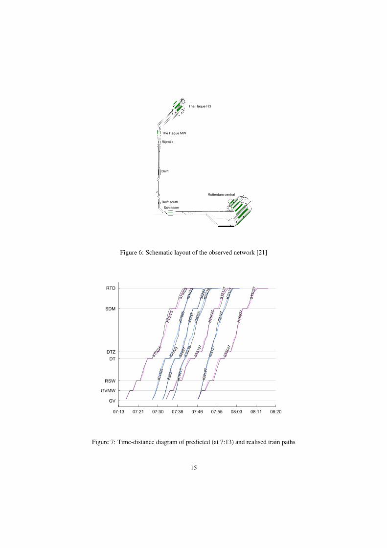
An example of predictions is shown in Figure 7. The presented time-distance diagramshows the predicted train paths (local trains are given in magenta and intercity trains inblue). The realised train paths in space and time are presented with black lines. The pre-diction is performed at the departure of train ST5025 from The Hague HS (GV). Completeroutes of the seven trains that enter the network within the 30 min prediction horizon areincluded in predictions. The average prediction error for 161 predicted events (includingsignal passages) is 19.33 s, while the maximum prediction error is 68.71 s. The maximumprediction error was produced for the passing time of a signal between stations Delft South(DTZ) and Schiedam (SDM) by train IC9216. The data set for that train line is significantlysmaller than for other lines due to its frequency (it runs only once in an hour while otherlines run every 30 min). We expect that the accuracy of predictions for that particular linewill improve when a larger training data set is considered.

The major advantage of the presented model for traffic controllers is the ability to pre-dict all route conflicts within the prediction horizon. We use the principle of overlapping

14

The Hague HS

The Hague MW

Rijswijk

Delft

Delft south

Schiedam

Rotterdam central

Figure 6: Schematic layout of the observed network [21]

ST5025

ST5025

ST5025

IC1925

IC1925

IC1925

IC1925

S2227

S2227

S2227

S2227

IC9216

IC9216

IC9216

IC9216

ST5127

ST5127

ST5127

IC2127

IC2127

IC2127

IC2127

ST5027

ST5027

ST5027

07:13 07:21 07:30 07:38 07:46 07:55 08:03 08:11 08:20

GV

RSW

DT

DTZ

SDM

RTD

GVMW

Figure 7: Time-distance diagram of predicted (at 7:13) and realised train paths

15

blocking times [12] to predict and visualise route conflicts.Figures 8 and 9 show the predicted and realised blocking time diagram respectively.

Local trains are presented in magenta and intercity trains in blue. Overlaps in blockingtimes that indicate route conflicts are given in red.

ST5025

ST5025

ST5025

IC1925

IC1925

IC1925

IC1925

S2227

S2227

S2227

S2227

IC9216

IC9216

IC9216

IC9216

ST5127

ST5127

ST5127

IC2127

IC2127

IC2127

IC2127

ST5027

ST5027

ST5027

07:13 07:21 07:30 07:38 07:46 07:55 08:03 08:11 08:20

GV

GVMW

RSW

DT

DTZ

SDM

RTD

Figure 8: Blocking time diagram predicted at 7:13

The three out of the four major route conflicts that occurred, one in Schiedam (SDM)and two in Rotterdam (RTD), were predicted by the model. However, the very short runningtime of IC2127 between stations Delft South (DTZ) and Schiedam (Figure 7) caused a routeconflict with the preceding ST5127 at SDM (Figure 9), which was not captured by the model(Figure 8).

Moreover, the chain of very short route conflicts at station Delft (DT) was not capturedbut only the conflict between IC9216 and ST5127. This example shows the morning peakhour which might cause longer dwell times in Delft and other short stops. Conditioning thedwell times on period of the day might improve these results. However, these inaccuraciesof the current model did not affect the predictions of arrival times in Rotterdam.

Computation time of the online prediction model in this example is very short (less thanone second). The model is therefore suitable for real-time applications with regular updatesof current train positions. For larger examples that model dense traffic, it is expectablethat more events can occur almost simultaneously, i.e., more than one update can arrivewithin one second. The presented event-driven prediction algorithm can easily be modifiedto a time-driven version where the prediction process is performed in regular time intervalsbased on the information that arrived within the interval.

16

ST5025

ST5025

ST5025

IC1925

IC1925

IC1925

IC1925

S2227

S2227

S2227

S2227

IC9216

IC9216

IC9216

IC9216

ST5127

ST5127

ST5127

IC2127

IC2127

IC2127

IC2127

ST5027

ST5027

ST5027

07:13 07:21 07:30 07:38 07:46 07:55 08:03 08:11 08:20

GV

GVMW

RSW

DT

DTZ

SDM

RTD

Figure 9: realised blocking time diagram

6 Summary and future work

This paper presents a microscopic model for accurate prediction of event times based on atimed event graph with dynamic arc weights. The process times in the model are obtaineddynamically using processed historical train describer data, thus reflecting all phenomenaof railway traffic captured by the train describer systems and preprocessing tools. The graphstructure of the model allows applying fast algorithms to compute prediction of event timeseven for large and busy networks.

The main contribution of our approach is the dynamic estimation of process times foreach train by using the predetermined functional dependence of process times on actual de-lays. Train interactions are modelled with high accuracy by including the main operationalconstraints and relying on actually realised corresponding minimum headway times (ob-tained from the historical data) rather than on theoretical values. The recursive depth-firstsearch algorithm with dynamic arc weights gives predictions for all event times within thehorizon.

The model has been applied in a case study on a busy corridor in the Netherlands in asimulated real-time environment, and produced accurate estimates for train traffic and routeconflicts within 30 min. Application of the model to a wider area is possible either byenlarging the observed area or by coordinating multiple areas. Finally, the model structureenables straightforward application of the network-wide delay propagation algorithm [8] toestimate the further effect of current traffic conditions (or examined traffic control actions).

The further research will be focused on investigating the impact of other factors, suchas period of the day and weather, on train running and dwell times. Factors with strong

17

impact on process times will be included in the prediction procedure in order to improve theaccuracy.

The predictive model provides effective decision support to signallers and traffic controland contributes to a better utilisation of railway infrastructure, improved reliability of trainservices, and more reliable and dynamic passenger information. The developed model willbe embedded in a closed-loop model-predictive railway traffic control framework whereonline optimization algorithms will automatically resolve detected conflicts and proposecontrol decisions to traffic controllers together with the predicted conflicts [14]. This wayan intelligent railway traffic management system will be obtained that pro-actively monitorsthe railway traffic and supports traffic controllers with decisions that optimize the traffic ona network level, beyond the traditional local control areas.

AcknowledgmentsThis paper is a result of the research project funded by the Dutch Technology FoundationSTW: “Model-Predictive Railway Traffic Management” (project no. 11025).

References

[1] Berger, A., Gebhardt, A., Muller-Hannemann, M., and Ostrowski, M. Stochastic De-lay Prediction in Large Train Networks. In Caprara, A. and Kontogiannis, S. (eds.),11th Workshop on Algorithmic Approaches for Transportation Modelling, Optimiza-tion, and Systems, pp. 100–111, Dagstuhl, 2011.

[2] Buker, T. and Seybold, B. Stochastic modelling of delay propagation in large networks.Journal of Rail Transport Planning & Management, 2(1-2):34–50, 2012.

[3] Corman, F., Goverde, R.M.P., and D’Ariano, A. Rescheduling dense train traffic overcomplex station interlocking areas. In Ahuja, R. K., Mohring, R. H., and Zaroliagis,C. D. (eds.), Robust and Online Large-Scale Optimization, vol. 5868 of Lecture Notesin Computer Science, pp. 369–386. Springer, Berlin, 2009.

[4] Daamen, W., Goverde, R.M.P., and Hansen, I.A. Non-Discriminatory Automatic Reg-istration of Knock-On Train Delays. Networks and Spatial Economics, 9(1):47–61,2008.

[5] D’Ariano, A., Pranzo, M., and Hansen, I.A. Conflict Resolution and Train SpeedCoordination for Solving Real-Time Timetable Perturbations. IEEE Transactions onIntelligent Transportation Systems, 8(2):208–222, 2007.

[6] Dolder, U., Krista, M., and Voelcker, M. RCS – Rail Control System – Realtimetrain run simulation and conflict detection on a net wide scale based on updated trainpositions. In Proceedings of the 3rd International Seminar on Railway OperationsModelling and Analyisis (RailZurich2009), pp. 1–15, Zurich, 2009.

[7] Exer, A. European Railway Signalling, chapter Rail Traffic Management, pp. 311–343. Institution of Railway Signal Engineers, A&C Black, London, 1995.

[8] Goverde, R.M.P. A delay propagation algorithm for large-scale railway traffic net-works. Transportation Research Part C: Emerging Technologies, 18(3):269–287,2010.

18

[9] Goverde, R.M.P. , Daamen, W., and Hansen, I.A. Automatic identification of routeconflict occurrences and their consequences. In Allan, J., Arias, E., Brebbia C.A.,Goodman C.J., Rumsey A.F., Sciutto, G., and Tomii, N. (eds.), Computers in RailwaysXI, pp. 473–482, Southampton, 2008. WIT Press.

[10] Goverde, R.M.P. and Meng, L. Advanced monitoring and management information ofrailway operations. Journal of Rail Transport Planning & Management, 1(2):69–79,2011.

[11] Hansen, I.A., Goverde, R.M.P., and Van der Meer, D.J. Online train delay recognitionand running time prediction. In Intelligent Transportation Systems (ITSC), 2010 13thInternational IEEE Conference on, pp. 1783–1788, Madeira, 2010.

[12] Hansen, I.A. and Pachl, J. (eds.). Railway Timetable & Traffic - Analysis, Modelling,Simulation. Eurailpress, Hamburg, 2008.

[13] Kecman, P. and Goverde, R.M.P. Process mining of train describer event data andautomatic conflict identification. In Brebbia, C.A., Tomii, N., and Mera, J.M. (eds.),Computers in Railways XIII, WIT Transactions on The Built Environment, vol. 127,pp. 227–238, Southampton, 2012. WIT Press.

[14] Kecman, P., Goverde, R.M.P., and van den Boom, T.J.J. A model-predictive controlframework for railway traffic management. In Proceedings of the 4th InternationalSeminar on Railway Operations Modelling and Analyisis (RailRome2011), pp. 1–15,Rome, 2011.

[15] Longo, G. and Medeossi, G. An approach for calibrating and validating the simulationof complex rail networks. In TRB 92nd Annual Meeting, pp. 1–19, Washington, 2013.

[16] Medeossi, G., Longo, G., and de Fabris, S. A method for using stochastic blockingtimes to improve timetable planning. Journal of Rail Transport Planning & Manage-ment, 1(1):1–13, 2011.

[17] Nachtigall, K. Time depending shortest-path problems with applications to railwaynetworks. European Journal of Operational Research, 83(1):154–166, 1995.

[18] Nash, A. and Huerlimann, D. Railroad simulation using OpenTrack. In Allan, J., C.A.Brebbia, R.J. Hill, Sciutto, G., and Sone, S. (eds.), Computers in Railways IX, pp.45–54, Southampton, 2004. WIT Press.

[19] Rousseeuw, P.J. and Driessen, K. Computing LTS Regression for Large Data Sets.Data Mining and Knowledge Discovery, 12(1):29–45, 2006.

[20] Siefer, T. and Radtke, A. Evaluation of delay propagation. In Proceedings of 7th WorldCongress on Railway Research, Montreal, 2006.

[21] Sporenplan. www.sporenplan.nl, 2013.

[22] Theeg, G. and Vlasenko, S. (eds.). Railway Signalling & Interlocking: InternationalCompendium. Eurailpress, Hamburg, 2009.

[23] Van der Aalst, W.M.P. Process mining: Discovery, Conformance and Enhancement ofBusiness Processes. Springer, Berlin, 2011.

19