Title: Decoding neural events from fMRI BOLD signal: A comparison of existing approaches and

development of a new algorithm

Authors:

Keith Bush

Department of Computer Science, University of Arkansas at Little Rock (UALR), Little Rock,

Arkansas, USA 72204

Josh Cisler

Brain Imaging Research Center, University of Arkansas for Medical Sciences (UAMS), Little Rock,

Arkansas, USA 72205

Corresponding Author:

Keith Bush

Address:

Department of Computer Science

University of Arkansas at Little Rock

2801 S. University Ave.

Little Rock, AR 72204

E-mail: kabush@ualr.edu

Phone: 501.569.8143

Fax: 501.569.8144

Short Title: Decoding neural events from fMRI BOLD signal

Keywords: deconvolution, fMRI, imaging analyses, BOLD, connectivity

1

Abstract

Neuroimaging methodology predominantly relies on the blood oxygenation level dependent

(BOLD) signal. While the BOLD signal is a valid measure of neuronal activity, variance in

fluctuations of the BOLD signal are not only due to fluctuations in neural activity. Thus, a

remaining problem in neuroimaging analyses is developing methods that ensure specific

inferences about neural activity that are not confounded by unrelated sources of noise in the

BOLD signal. Here, we develop and test a new algorithm for performing semi-blind (i.e., no

knowledge of stimulus timings) deconvolution of the BOLD signal that treats the neural event as

an observable, but intermediate, probabilistic representation of the system’s state. We test and

compare this new algorithm against three other recent deconvolution algorithms under varied

levels of autocorrelated and Gaussian noise, hemodynamic response function (HRF)

misspecification, and observation sampling rate (i.e., TR). Further, we compare the algorithms’

performance using two models to simulate BOLD data: a convolution of neural events with a

known (or misspecified) HRF versus a biophysically accurate balloon model of hemodynamics.

We also examine the algorithms' performance on real task data. The results demonstrated

good performance of all algorithms, though the new algorithm generally outperformed the

others (3.0% improvement) under simulated resting state experimental conditions exhibiting

multiple, realistic confounding factors (as well as 10.3% improvement on a real Stroop task).

The simulations also demonstrate that the greatest negative influence on deconvolution

accuracy is observation sampling rate. Practical and theoretical implications of these results for

improving inferences about neural activity from fMRI BOLD signal are discussed.

2

1 Introduction

Functional magnetic resonance imaging (fMRI) is the predominant methodology of

contemporary neuroimaging and is most commonly performed using blood oxygenation level

dependent (BOLD) contrast [1]. BOLD imaging is founded on neuronal activity-dependent

changes in local magnetic fields. Neuronal activity is followed by a reliable influx of oxygenated

hemoglobin molecules that alters the ratio of oxygenated:deoxygenated hemoglobin molecules

in the local blood supply. This local change in magnetic field is the basis of the BOLD contrast

mechanism: differences in detected signal between two states (e.g., viewing faces versus no

stimulation) reflect differences in local oxygenated:deoxygenated hemoglobin ratios, which in

turn reflect differences in neural activity. While the exact physiological mechanisms mediating

the BOLD contrast mechanisms are not clear, research has demonstrated that the BOLD signal

is strongly correlated with local field potentials [2] and is a valid, though indirect, measure of

neural activity [3,4].

The mediating hemodynamic response exploited in the BOLD contrast mechanism is

referred to as the hemodynamic response function (HRF). The canonical model of the HRF

resembles a gamma function, with a delayed time to peak of about 6 seconds following

neuronal activation, which is followed by a slow return below baseline (referred to as the

postimulus undershoot) for about 10 seconds that gradually returns to baseline. The HRF is a

delayed and slow process due to physiological constraints on blood flow, the metabolic rate of

oxygen, and cerebral blood volume (e.g. [5]); thus, there is a temporal delay between the

theoretically-predicted neural events and the observed time to peak of the HRF. Further, given

3

that the HRF is an indirect measure of neuronal activity dependent on other physiological

processes in addition to neuronal firing, fluctuations in the BOLD signal are not only due to

fluctuations in neuronal events. A classic example of the limitations of the HRF as a measure of

neuronal events comes from a seminal study by Glover [6] where he demonstrated that the

BOLD signal arising from series of stimuli could be clearly deconvolved only when they were

separated by at least 4 s. That the BOLD signal arising from stimuli separated by less than 4 s

could not be clearly deconvolved is consistent with the physiological constraints on the HRF

predicted by Buxton's and colleagues' [7] balloon model of blood flow and oxygenation. This

example highlights the fact that observations of the signal (BOLD) are influenced by more than

just the source of interest (neural activity); thus, inferences about neural activity derived from

observations of the BOLD signal are potentially confounded by the extraneous influences.

The inherent limitations of the HRF as a multidetermined and regionally-varying signal

has been at the center of a recent controversy in neuroimaging analyses [8,9,10] regarding the

importance and validity of deconvolution. The controversy was started from a study by David et

al. [11], who compared the accuracy of network connectivity tested with Granger causality

analyses (where deconvolution was not performed) and dynamic causal modeling (where

deconvolution is implied within its state-space model) of fMRI measurement with respect to

network connectivity observed with EEG measured simultaneously with the fMRI. The results

demonstrated that models defined from fMRI measurement were only accurate when

deconvolution was performed. Similarly, a recent simulation study comparing modeling

approaches to characterizing network connectivity demonstrated that Granger causality

approaches detected true underlying causality with only chance accuracy [12], the implication

4

being that because Granger causality analyses are based on an autoregressive lag model, the

diffuse and multidetermined nature of the HRF corrupts the ability of Granger analyses to

detect causality. Connectivity analyses are not the only methods potentially confounded by

extraneous influences on the HRF: functional activation studies have a long history of attempts

to correct for inter-individual and interregional variation in the shape of the HRF when

convolving the stimulus timings to create predictors of the BOLD signal (e.g., through basis

functions or inverse logit estimation [13,14]). Debate has subsequently ensued about whether

the BOLD signal should be deconvolved prior to analyses given imperfect methods of

deconvolution [8,9,10]. That is, theoretically, deconvolution of the BOLD signal into its

mediating neural events will improve inferences about neural activity; however, actual

deconvolution may introduce its own source of error that is not necessarily less than the error

for which it is intended to correct [9].

Given the agreed upon possibility of hemodynamic deconvolution as a potential solution

to the limits of the BOLD signal as an indirect measure of neuronal activity, efforts should be

directed toward developing theoretically and empirically supported deconvolution algorithms.

The optimal deconvolution algorithm would not be dependent on knowledge of the stimulus

timings, otherwise the algorithm would not be applicable to studies with no stimulus timings

(resting-state studies) or studies with unknown or unreliable stimulus timings. Here, we present

a promising step toward optimizing deconvolution of fMRI BOLD signal that extends the recent

state-of-the-art attempts at deconvolution [15,16,17]. Hernandez-Garcia and Ulfarsson [17]

developed a deconvolution algorithm that inverts, iteratively, a linear system regularized in

three-parts: 1 [18], total variation [19], and non-negativity. While their algorithm was an

5

important advance in this area, it suffered from several limitations including suboptimal

detection accuracy under moderate levels of Gaussian noise, suboptimal accuracy in detecting

events from real-world event-related design-derived BOLD signal, and lack of accounting for

neural influences preceding the observed BOLD timeseries. A related algorithm, utilizing

self-tuned ridge regression, was proposed by Gaudes et al. [16]; however, this algorithm was

not validated on a theoretical model of BOLD making direct comparisons to other algorithms

difficult. An additional limitation common to regression-based approaches is the use of an

unrealistic theoretical model of neuronal activity during algorithm validation: modeling

neuronal events at 1 Hz frequency while also observing neural activity at 1 Hz frequency. Neural

events occur at a much higher frequency (e.g., 100 Hz) than the typical sampling rate of fMRI

(e.g., .5 Hz). Havlicek and colleagues [15] developed a method of truly blind deconvolution

based on cubature Kalman filtering (approximate Bayesian filter) that utilizes stochastic

differential equations describing a state-space model of the HRF (e.g., including vascular,

metabolic, and neural sources of variance) to provide estimates of neuronal activity. While this

approach exhibits many significant theoretical advantages (including modeling of neural events

at generation rates faster than observations rates), it relies on a complex set of assumptions

concerning the dynamical behavior of the HRF, and its robustness to realistic levels of noise has

not been tested.

We structure the manuscript into four parts. First, we describe a computational model

of BOLD signal generation and observation which provides a general framework for unifying

performance results reported in the deconvolution literature. Second, we derive a novel

deconvolution algorithm designed to exploit robust characteristics of existing algorithms while

6

also overcoming some of their intrinsic limitations. Third, we describe and execute a set of

experiments that examine the performance of state-of-the-art BOLD signal deconvolution

algorithms via simulation. Each experiment precisely controls, via computational model, factors

that confound real-world BOLD signal observations. From these experiments we verify

previously reported results and compare performances across widely disparate algorithms,

including our novel algorithm. Finally, we combine experimental results to gain deeper

understanding into the problems of practical application of deconvolution, propose potential

solutions, and offer guidance on fruitful directions of future research.

2 Methods

Our methods are comprised of (1) a comprehensive parametric computational model of fMRI

BOLD signal generation, (2) a novel algorithm for deconvolution of neural events, as well as (3)

a collection of state-of-the-art deconvolution algorithms against which we compare our

algorithm and assess limitations of deconvolution in practical application.

2.1 A Generative Model of fMRI BOLD

Following prior simulation models [20,21], we construct a model of resting state neural activity

using standard assumptions about the nature of the observed BOLD signal. It is important to

note that this model could also be extended to simulate task-based data (if assumptions about

and models of the temporal distribution of neural events generated by a given task could be

7

identified); however, we chose first to focus on resting-state data to necessitate deconvolution

in the absence of stimulus timings. As such, any algorithm that is effective on resting-state data

would also be effective on task data, but not necessarily vice versa. We model fMRI BOLD signal

in three distinct processes: (1) a signal generation process that captures temporal structure of

neural events; (2) a theoretical BOLD generation process that maps neural events onto an ideal

BOLD signal (using either the canonical HRF or the balloon model); and, (3) an observation

process that maps theoretically ideal BOLD signals onto low-frequency, noise-corrupted BOLD

observations that represent real-world signals. These three systems, combined, we call the

model. We describe each of these processes below.

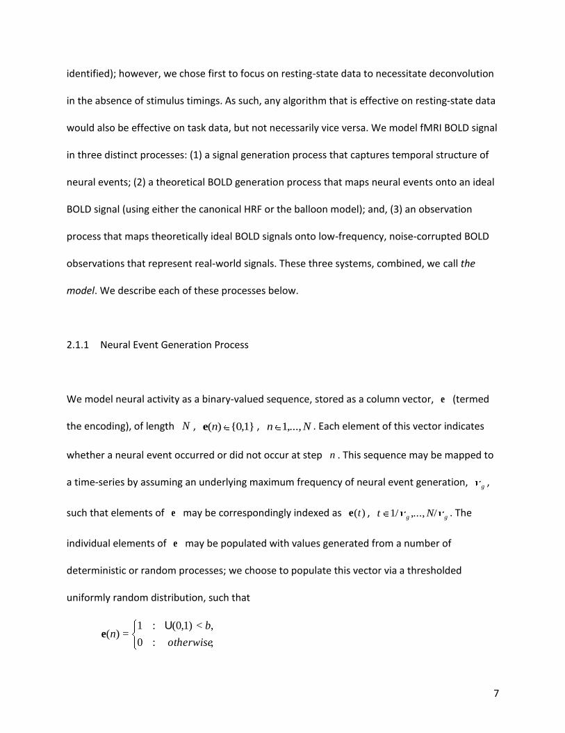
2.1.1 Neural Event Generation Process

We model neural activity as a binary-valued sequence, stored as a column vector, e (termed

the encoding), of length N , {0,1})(ne , Nn 1,..., . Each element of this vector indicates

whether a neural event occurred or did not occur at step n . This sequence may be mapped to

a time-series by assuming an underlying maximum frequency of neural event generation, g

,

such that elements of e may be correspondingly indexed as )(te , gg Nt /,...,1/ . The

individual elements of e may be populated with values generated from a number of

deterministic or random processes; we choose to populate this vector via a thresholded

uniformly random distribution, such that

,:0

,<(0,1):1=)(

otherwise

bn

Ue

8

where b is the fraction of neural activity desired in the model, [0,1]b .

2.1.2 Mapping of Neural Events to BOLD response

We generate the true (i.e., theoretical ) BOLD signal of the neural event encoding in either of

two ways: via canonical HRF or via a more biophysically sophisticated hemodynamic model

based on Buxton’s balloon model [7,22,15]. The canonical HRF1 approach is predicated on a

kernel vector, k , of length K . We convolve this kernel with the encoding to form an element

of the true BOLD signal, x , at time, t :

.1))(()(=)(1=

ititK

i

ekx

This formulation is identical to convolution via Toeplitz matrix [16,17] but is preferred due to

computational limitations of the explicit matrix form.

Alternatively, the encoding may be used as the input, u , to a nonlinear dynamical

model of hemodynamics, widely utilized in fMRI simulation and analysis, termed the balloon

model [7]. In this approach a system of differential equations governing the physiology of

hemodynamics is numerically integrated to yield the true BOLD signal. In this work we utilize

the exact algorithm (state initialization and numerical integration codes) reported in Havlicek et

al. [15], which may be summarized as follows. Given a system of differential equations

governing hemodynamics and a set of realistic parameters for these equations:

1. convolve the encoding, e , with a Gaussian kernel to form neural hemodynamic

influences, u ,

1 We used the canonical HRF as provided in the commonly used SPM software package.

9

2. initialize the system state to zero,

3. numerically integrate the system of differential equations [7], incorporating external

influences, u , to yield a time-course of the system’s state, s , and

4. compute the true BOLD signal, x , as a function of the system state: )(= sx f .

As we have defined the encoding vector’s indexing in terms of both samples, Nn , and time

points, Tt (with the conversion between the two being the frequency of neural event

generation, g

), we impose no lower bound on numerical integration time-step, t . This is

important to note, given the role of step-size in the error propagated within a dynamical

system’s state-space via integration. For the purposes of this work, we only require that the

numerical integration step-size be less than or equal to g1/ , which ensures the impact of

neural event timings on the temporal evolution of the true BOLD signal is consistent with the

canonical HRF convolution.

2.1.3 Observation Process

BOLD signals that mimic real-world measurement complexities are created via an observation

process. In the model this process is composed of a series of mappings, each parameterized to

reflect one of a range of assumptions concerning how true BOLD signals are converted into

observed BOLD signals in practice. Each mapping is either present or not present in the

observation process of a simulation. Moreover, if a mapping is selected to be included in the

observation process then there may also be one or more parameters associated with this

mapping specifying the degree of the effect. Currently, the observation process contains the

10

following mappings.

Latent neural activity: BOLD signals observed directly from the brain are the result of a

continuous neural generation process and include the influence of neural events that occurred

prior to the start of observation, i.e., latent neural events. In the simulation the K th element

of the true BOLD signal is the first element for which the distribution of these latent neural

events are stationary; therefore, to simulate latent neural events that occur in real-world

observations, the first K-1 elements should be removed. We decompose the N elements of

the true BOLD response x , into two sequences of length 1K and M , respectively, such

that MKN 1)(= : 1):(1= Ktrans xx , which we term the transient signal (which is

discarded); and, ):(= NKobs xx , which we term the observed BOLD signal. If this mapping is

not utilized in the observation process then xx =obs .

Physiological variation: Unexplained variation in the underlying physiological process cannot be

removed (independent of changes to measurement equipment) and is always included in the

model. Physiological noise is well-known to be temporally correlated due to confounding

factors such as cardiac and respiratory signals. We simulate this process as a first-order

autoregressive, AR(1), signal [23,24], phys , comprised of zero-mean white Gaussian noise and

correlation coefficient, ρ:

,0,1(0) ,1,..., ,0,11)(=)( NN physphysphys Miii

which is normalized to the standard score and then scaled according to a signal-to-noise ratio

11

parameter,

,=phys

obsx

physphysSNR

where parameter obs

x is the mean of obsx . The noise process is then added to the

observation,

physobsobs xy = ,

to form the physiologically noise corrupted signal, obsy .

Downsampling: The observation process is parameterized by a frequency of observation, o

(note, oTR 1/= ). We first compute the downsampling rate, d , using the function ogd /= .

In this work we assume always that og

and that g

is evenly divisible by o . Under

these assumptions, Zd and 1d . We then downsample the observed BOLD signal,

,1,..., ,)(=)( Piidi obsdsmp yy

to form the downsampled observed BOLD signal, dsmpy , of length, dMP /= . If this mapping is

not used then obsdsmp yy = , implying 1=d and MP = .

Measurement noise: Unexplained variation due to underlying stochastic processes in the

measurement may or may not be altered through changes to or modification of measurement

equipment. Therefore, we model this process independently of the model of physiological

variation, and we assume that it is comprised of a zero-mean white Gaussian noise signal such

that

12

,= scandsmpscan yy

where,

,1,..., ,0,=)( PiSNR

iscan

dsmpy

scan N

where dsmp

y is the mean of

dsmpy and scanSNR is the signal-to-noise ratio of the

measurement equipment. If this mapping is not included in the observation process then

dsmpscan yy = .

Normalization: BOLD signal is measured in dimensionless units; therefore, it is the relative

change of the signal through time that provides key information about underlying neural

activity. Normalization of the observed BOLD signal, either on a scale of percent signal change

or a standard normal distribution (zero mean and unit variance), is nearly universal. If this

mapping is included in the observation process then we compute the normalized observed

vector, scany , as

,)(= scanscan z yy

where )(z is the normalization function. If this mapping is not included then scanscan yy = .

Combined, the five mappings presented above form a simulation of the observation

process that converts a true BOLD signal into a noise-corrupted, downsampled BOLD

observation. It is on these corrupted signals that we (by varying the presence, absence, or

magnitude of the different mappings composing the observation process) evaluate and

compare the accuracy and robustness of deconvolution algorithms.

13

2.2 A novel deconvolution algorithm

Using the model as a surrogate for the complexities of real-world fMRI observations, we derive

two important insights about the nature of deconvolution. First, deconvolution algorithms

should explicitly optimize representations of neural event encodings that are strictly positive;

allowance of both positive and negative neural event encodings is physiologically unsupported

and needlessly introduces symmetry into the solution space that could, potentially, introduce

overfitting in response to latent factors.

Second, it is the intensity of neural activity (convolved with the HRF), rather than neural

event timing, that dominates temporally promixal BOLD signal variance. We demonstrate this

via multiple random simulations of two different models in which neural events are generated

at 100Hz and the resultant BOLD signal is sampled at 1Hz (noise and normalization are

omitted). Figure 1, panel (a), depicts temporal distributions (computed over 30 random

simulations) of the sampled BOLD signals: the solid-lined distribution captures BOLD signals

generated by the model when 2% activity occurs within the 3rd second of observation; the

dash-lined distribution represents BOLD signals generated when 4% neural activity occurs

within the 13th second of observation. Panel (b) depicts the timing of aggregate neural activity

(i.e., the number of neural events divided by the number of time-points within an observation

interval).

Figure 1 demonstrates that observed signal variance induced by low-frequency sampling

of a BOLD signal generated from high-frequency neural events is small relative to signal

14

variance induced by the shape of the HRF and the number of neural events occurring within an

observation. Thus, random rearrangement of the timing of neural events within a (relatively)

short observation window generates less variation in the observed BOLD signal than the

number of neural events that occur (signal variance scales linearly with the number of events).

Therefore, it is reasonable for a deconvolution algorithm to model neural events at the rate of

observation (rather than at the rate of generation) as long as the magnitude of neural activity

within a discrete time-interval is captured.

Our algorithm is designed to leverage both of these insights by modeling neural events

(i.e., the encoding) as a vector of continuous values strictly on the range (0,1) . To achieve this,

we first model measured BOLD as a vector, y~ , of length T , given by:

)(=~ Fhy z (1)

where F is a feature matrix of size KT , h is the HRF kernel column-vector of length K ,

and )(z is the normalization mapping.

The feature matrix, F , is a modification of the Toeplitz matrix, such that

,:0

1,..., ,,...,2 ,>:~

=),(otherwise

KkMKiKkikiki

eF

(2)

where e~ is the encoding: a vector of length 1)(KM , (0,1))(~ te , MKt ,...,2 . Each

element of this vector represents the magnitude of neural activity (a value 0.5 equates to mean

neural activity, whereas 0 and 1.0 represent minimum and maximum neural activity,

respectively). It may be helpful to imagine matrix F as a mapping that distributes influences

of neural events through time (including neural events that occur before the start of

observation).

15

To achieve the desired range of )(~ te the deconvolution algorithm assumes that neural

events are driven by an unobserved time-series of real-valued neural activations, a , R)(ta ,

TKt ,...,2 , that are temporally independent and whose values determine the neural event

encoding via the logistic function,

.))((1

1=)(~

texpt

ae

Using this model, we deconvolve the BOLD observations by optimizing neural activations, a ,

such that they minimize the cost function, J , given by

.):(1~

2

1=

2

scanM yyJ

(3)

This optimization may be achieved via backpropagation of errors where the contribution of the

neural activations, a , to the cost, J , is computed via the chain rule,

.~

~)(

)(

~

~=a

e

e

F

F

y

y

J

a

J z

z (4)

In this paper we apply a simplifying assumption that the normalization operator influences,

primarily, the magnitude of the gradient, and has only minimal influence on the direction,

therefore,

.~)(

)(

~

F

Fh

Fh

y

F

y z

z (5)

We then evaluate the derivative of the cost with respect to the neural activation, a , and take a

small step, , in the opposite direction,

.=aa

Jaa

(6)

Iterative application of Equation 6 will converge to a locally minimum solution to Equation 3. In

16

practice, iteration continues until a termination criterion is met.

To facilitate fast convergence of gradient descent, we initialize the neural activation to a

high-quality solution. An excellent initial solution is given by values of a that have been

pre-solved to generate an encoding that is equivalent to the observed BOLD signal, scany ,

scaled to the range [0,1] and shifted by the time-to-peak of the assumed HRF kernel.

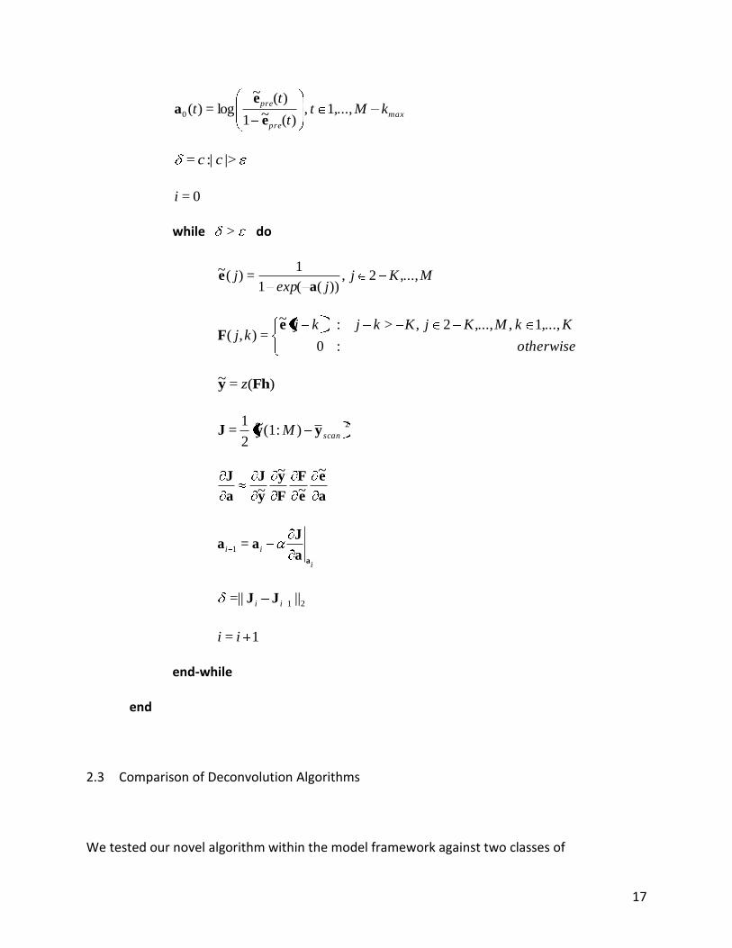
Algorithm 1 describes the computational steps of this initialization process as well as the full

gradient descent loop. The key insight to take away from Algorithm 1 is that the neural

activation parameters, a , over which the cost function is optimized, are not the quantities of

interest. Rather, it is the logistically saturated representation of these parameters, the vector

e~ , that represents estimated neural events and is the target of deconvolution.

Algorithm 1: Observed BOLD signal deconvolution

parameters: , , Kkk ,...,1 ,)(: Rhh

data: Mttscanscan ,...,1 ,)(: Ryy

result: MKjj ,...,2 ,(0,1))(~:~ ee

begin

Kkkrgmaxkkmax 1,..., ,1))((a= h

Mttt scanscanadj 1,..., ,)(min)(=)( yyy

maxadjmaxadjpre kMtktt 1,..., ,)(max)/(=)(~ yye

MKjj ,...,2 ,0=)(0a

17

max

pre

prekMt

t

tt 1,..., ,

)(~1

)(~

log=)(0e

ea

|>:|= cc

0=i

while > do

MKjjexp

j ,...,2 ,))((1

1=)(~

ae

otherwise

KkMKjKkjkjkj

:0

1,..., ,,...,2 ,>:~

=),(e

F

)(=~ Fhy z

2

):(1~

2

1= scanM yyJ

a

e

e

F

F

y

y

J

a

J ~

~

~

~

i

ii

aa

Jaa =1

21 ||=|| ii JJ

1= ii

end-while

end

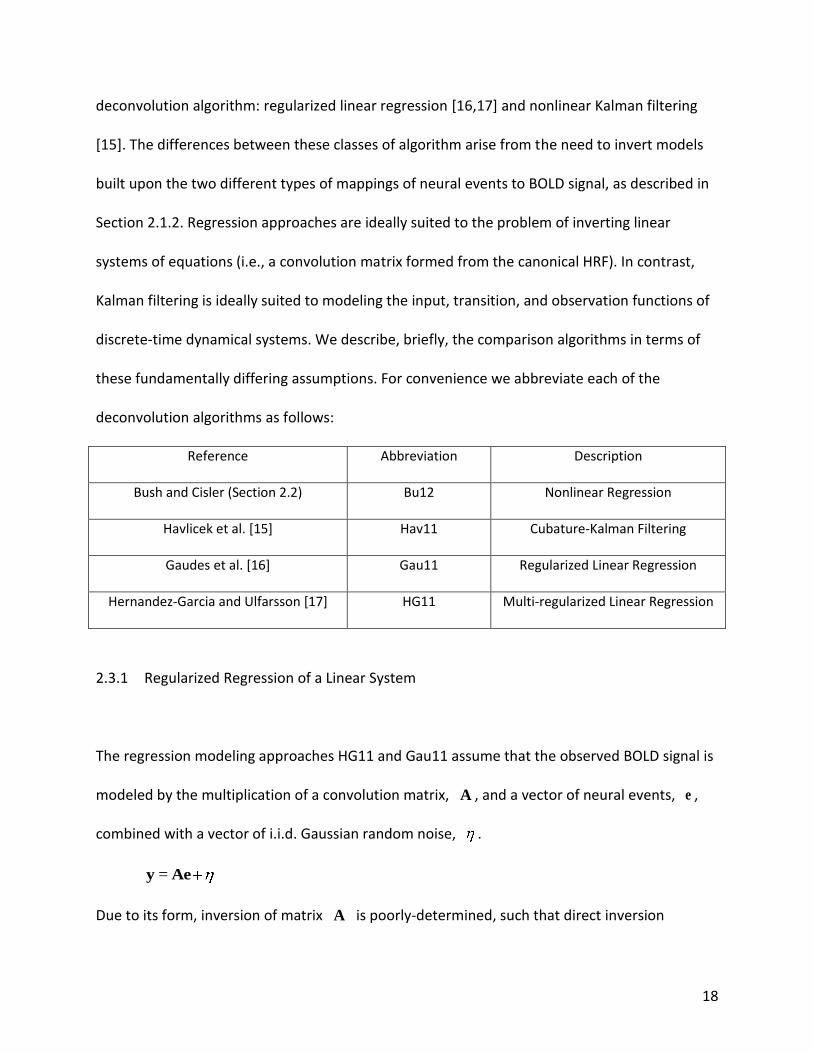
2.3 Comparison of Deconvolution Algorithms

We tested our novel algorithm within the model framework against two classes of

18

deconvolution algorithm: regularized linear regression [16,17] and nonlinear Kalman filtering

[15]. The differences between these classes of algorithm arise from the need to invert models

built upon the two different types of mappings of neural events to BOLD signal, as described in

Section 2.1.2. Regression approaches are ideally suited to the problem of inverting linear

systems of equations (i.e., a convolution matrix formed from the canonical HRF). In contrast,

Kalman filtering is ideally suited to modeling the input, transition, and observation functions of

discrete-time dynamical systems. We describe, briefly, the comparison algorithms in terms of

these fundamentally differing assumptions. For convenience we abbreviate each of the

deconvolution algorithms as follows:

Reference Abbreviation Description

Bush and Cisler (Section 2.2) Bu12 Nonlinear Regression

Havlicek et al. [15] Hav11 Cubature-Kalman Filtering

Gaudes et al. [16] Gau11 Regularized Linear Regression

Hernandez-Garcia and Ulfarsson [17] HG11 Multi-regularized Linear Regression

2.3.1 Regularized Regression of a Linear System

The regression modeling approaches HG11 and Gau11 assume that the observed BOLD signal is

modeled by the multiplication of a convolution matrix, A , and a vector of neural events, e ,

combined with a vector of i.i.d. Gaussian random noise, .

Aey =

Due to its form, inversion of matrix A is poorly-determined, such that direct inversion

19

methods, i.e., yAe1=~ , will have difficulty producing a good encoding estimate, e~ . To

overcome this weakness the cost function of the regression necessarily includes a regularization

term, , such that

,)~(||~=|| eyeAJ

which enforces an intended structure on the estimated encoding, e~ . The fundamental

difference between the regression-based comparison algorithms is the form of the

regularization, .

The inversion method promoted in Gau11 is regularized generalized least-squares (i.e.,

ridge regression) in which the regularization parameter is tuned from statistical properties of

the dataset [25]. In contrast HG11 incorporates a regularization term composed of the sum of

three parameterized penalty terms included to respectively promote, but not strictly enforce,

encoding solutions that are sparse, piece-wise constant, and positive-valued. The form of the

regularization does not permit a generalized least squares solution, and, therefore, the authors

use majorization-minimization to find the minimum of the cost function and solve for e~ .

2.3.2 Cubature-Kalman Filtering of a State-Space Model

The Hav11 algorithm employs cubature Kalman filtering to infer an estimate of neural activity

(i.e. latent variables) from the interaction between evidence (the observed BOLD signal) and a

system of stochastic differential equations that describe the temporal evolution of vascular,

metabolic, and neural sources of variance (the balloon model).

Given an estimate of the initial state of the observed system’s physiology, Kalman

20

filtering utilizes statistical inference to optimally estimate the unobserved neural events.

Kalman filtering was originally derived for linear systems [26]. It was later extended to

nonlinear dynamical systems [27,28]. Cubature Kalman filtering [29] is a mathematically distinct

and theoretically more accurate variation of nonlinear Kalman filtering. We direct the reader to

an exhaustive derivation of the hemodynamic filter in Havlicek et al. [15].

There are theoretical advantages of the Kalman filtering approach over regression

methods. First, Kalman filtering holds the potential for truly “blind” deconvolution by

simultaneously estimating the state of the system (i.e., the physiological state), the unknown

neural event timings, as well as the physiological parameters driving the hemodynamic

response. Thus, Kalman filtering can adjust its estimate of the encoding vector for subject- and

region-specific hemodynamic variation (e.g. time-to-peak), which is well-known to exist in

practice [28,29].

2.4 Example Simulation and Deconvolution

To illustrate the experimental methods utilized in this paper, each step of the generation,

observation, and deconvolution process for a simulation (i.e., trial) has been plotted to Figure 2.

Parameters for this trial are as follows: the total number of observations was 200, neural

activity is 5%, 20=g Hz, 1=o Hz, 6=physSNR , 9=scanSNR , and neural events are

mapped onto the BOLD signal via the canonical HRF (time-to-peak 6 s).

Figure 2 panel (a) depicts the timings of randomly sampled neural events temporally

aligned with the true BOLD signal scaled on the range [0,1] . Panel (b) depicts the same signal

21

corrupted by noise, where the first K-1 observations are removed, and the result observations

are normalized. Panel (c) depicts the encodings predicted by each of the deconvolution

algorithms that assume the canonical HRF: HG11, Gau11, and Bu12. These predicted encodings

have been scaled to the range [0,1] .

3 Experiments

Our experiments compared the performance and robustness of deconvolution algorithms. We

made these comparisons by empirical analysis of each algorithm’s ability to accurately detect

timings of neural events from resting state fMRI BOLD signal. Due to the nature of resting state

BOLD signal, it was technically infeasible to obtain ground truth neural event timings in vivo.

The model, described in Section 2, provided both the observations and ground truth for resting

state analysis.

The mechanism by which we simulated real-world data was the observation process,

which allowed us to confound the observed BOLD signal through inclusion or exclusion of latent

neural events, corruption by noise, scale effects, and removal of temporal information

(downsampling). A convenient way to describe the experiments is to describe the default

configuration of the model and then identify each experiment’s deviation from it.

We performed seven sets of experiments (27 experiments total) designed to

systematically (and incrementally) introduce complexity into the observation process of the

model. These experiments allowed us to explore, compare, and understand the strengths and

weaknesses of the various mathematical approaches to deconvolution in response to

22

confounding factors exhibited by real BOLD signals.

We begin by describing the default model. The default model generated 200

observations (generated at 1Hz and observed at 1Hz) and was configured to exhibit 5% neural

activity ( 0.05=b ). The canonical HRF exhibited a time-to-peak of 6 seconds and the balloon

model exhibited the default physiological parameters as described in Havlicek et al. [15]. The

true BOLD signal was not corrupted by noise (neither physiological nor scanner) and the

observed BOLD signal was normalized. For each experimental configuration, reported below,

the model generated 30 random neural event sequences and (where appropriate) 30 random

observation processes.

3.1 Latent Neural Events

Experiments 1 and 2 examined the effects of latent neural events (see Section 2.1.3).

Algorithms based on the convolution matrix (Gau11 and HG11) do not account for latent

variables; however, the Bu12 algorithm explicitly models latent neural events in its feature

matrix (see Eqn. 2). To test the influence of latent neural events on deconvolution performance,

we require the algorithms to deconvolve the full observation sequence (Experiment 1) and then

have them deconvolve observation sequences with the first K-1 observations removed

(Experiment 2). The first K-1 observations are also removed in Experiments 3–23.

3.2 Measurement Noise

23

Experiments 3–6 examined the effect of noise on deconvolution accuracy. As described in

Section 2, the model’s observation process included two layers of noise: physiological noise,

physSNR , and scanner noise, scanSNR . These experiments fixed 6=physSNR (see Experiment 23

for origins of the SNR values) and varied scanner noise 0}{3,5,10,10scanSNR .

3.3 Observation rate (TR) relative to generation rate

Experiments 7–12 examined the role played by the observation rate with respect to the

frequency of neural event generation in the absence of noise. As mentioned in the introduction

and empirically demonstrated in Figure 1, it is a harder analytical problem to deconvolve neural

events generated at a higher frequency than the observation sampling rate. These experiments

fixed the observation frequency to a realistic value 1=o Hz (reminder, TR = o1/ ) and

varied the frequency of neural event generation 20,40}{1,2,5,10,g Hz.

3.4 Misspecification of HRF

Experiments 13–16 examined the role that HRF misspecification plays in deconvolution

accuracy. To test this impact we adapted the model of hemodynamic variability proposed in

Havlicek et al. [15]. The model was configured such that it maps neural events to BOLD signal

via the balloon model; for each random trial of the experiment, the model sampled uniformly

randomly from biologically plausible ranges of physiological parameters of this model according

to Havlicek et al. [15]. It is important to note that the mean of the parameter ranges of the

24

balloon model used by Havlicek et al. [15] generated an HRF with time-to-peak 4 s. By default,

algorithms HG11, Gau11, and Bu12 assume the canonical HRF (the default in SPM software),

which peaks at 6 s. Therefore, for these experiments only, we modified the time-to-peak of the

canonical HRF to be 4 s to facilitate comparisons between algorithms. This experimental set-up

provided us with an approximate mechanism for quantifying the cost of HRF misspecification in

deconvolution accuracy within and across algorithms. It also allowed simultaneous investigation

of the joint influence of HRF misspecification and scanner noise, which the experiments varied,

respectively, 0}{3,5,10,10scanSNR .

Similarly, Experiments 17–22 examined the interaction between HRF misspecification

and the ratio of TR to the rate of neural event generation. The observation rate was fixed,

1=o Hz, and the generation rate, g

, varied across experiments, 20,40}{1,2,5,10,gHz.

3.5 Realistic resting state simulation parameters

Experiment 23 tested deconvolution performance of the algorithms under conditions that

simulate real-world BOLD observations: latent neural events, random misspecification of the

HRF, highly-correlated and high-amplitude physiological noise ( 75.0= and 6=physSNR ),

scanner noise ( 9=scanSNR ), and large disparity between neural event observation and

generation rates ( 1=o Hz and 20=g Hz). The magnitudes of physiological and scanner

noise were determined by ratios calculated in [30]. The magnitude of the physiological

process's autocorrelation was taken from [23,24].

25

3.6 Real Task Data

Experiment 24 tests deconvolution performance of the algorithms using real-world fMRI BOLD

data acquired from an adult male while performing an event-related design; this provided a test

of how well the algorithm does under real life conditions (e.g., unknown noise, unknown HRF,

randomly jittered interstimulus interval (ISI), subject fatigue, corrected head movement, etc.). A

Philips 3T Achieva X-series MRI system using an 8-channel head coil (Philips Healthcare,

USA) was used to acquire imaging data. Anatomic images were acquired with a MPRAGE

sequence (matrix=192x192, 160 sagittal slices, TR/TE/FA=min/min/900, final

resolution=1x1x1mm3 resolution). Echo planar imaging sequences were used to collect the

functional images using the following sequence parameters: TR/TE/FA=2000ms/30ms/900,

FOV=240x240mm, matrix=80x80, 37 oblique slices (parallel to AC-PC plane to minimize OFC

sinal artifact), slice thickness=3 mm, final resolution 3x3x3 mm3. All research protocols with

human subjects were done with approval of the institutional review board. The subject

performed four 8 minute runs of a pictorial Stroop task with the ISI jittered randomly to vary

between 3 and 8 seconds and with a fixation cross occurring in between stimulus presentations.

Time-courses from a cluster of 32 voxels were extracted separately for each of the four runs

from a region in the ventral occipital lobe that showed significant task activation.

3.7 Comparisons to Havlicek et al. algorithm

26

Experiments 25–27 modified the parameters of the model to facilitate direct comparison

between the HG11, Gau11, Bu12, and Hav11 algorithms. The Hav11 algorithm and parameters,

as implemented in Havlicek et al. [15], are not designed to handle time-series of significant

length in practice (e.g., 200 s) or with the types of confounding factors we include in this work

(primarily due to the algorithm's estimation of the underlying signal at ten times higher than

observed); thus, to facilitate valid comparisons among all algorithms, we configured the model

to exactly reproduce the simulation configuration reported in Havlicek et al. [15]. Specifically,

latent neural events were not removed, the observations were not normalized, the length of

the time-series was fixed to 40 s, 1=o Hz, 10=g Hz, and the balloon model (an

underlying assumption of the Hav11 algorithm) was used within the model (rather than the

canonical HRF) to map neural events to the BOLD signal. One specific difference in these

experiments was that we included 5% randomly sampled neural activity rather than a small set

(4) of neural events.

Using these simulation parameters, Experiment 25 compares deconvolution

performance across the four algorithms omitting physiological and scanner noise; also, the

parameters of the balloon model are assumed to be known. Experiment 26 is identical to

Experiment 25 except that parameters of the balloon model are unknown and sampled

randomly according to the methodology described for Experiments 13–22 (Experiment 26 is in

fact identical to the configuration of the experiment reported in Havlicek et al. [15] except for

the random sampling of neural events). Experiment 27 is identical to Experiment 26 but

includes more realistic levels of noise: 75.0= , 6=physSNR , and 9=scanSNR . Note, the

Hav11 algorithm in Experiment 27 is configured to estimate the observational noise using a

27

variational Bayesian approach.

3.8 Deconvolution Algorithm Source Code and Parameters

Original source codes for the HG11, Gau11, and Hav11 algorithms were incorporated into the

experimental codes in this work via wrapper functions. Due to the complexity of the various

codes, their assumptions, and their parameters, which may have bearing on the interpretation

of these experiments, we refer the reader to these algorithms’ respective parametric details

[15,16,17] and the respective codes, which we deviated from only twice. Within experiments

investigating misspecification of the HRF (Experiments 13–22), we modified the time-to-peak of

the HRF kernel to be 4 s in the HG11 and Gau11 (and Bu12) algorithms. In Experiment 27, we

corrupted the observed BOLD signal with noise (which was not part of the original validation of

the Hav11 algorithm [15]). For all experiments the Bu12 algorithm learning parameters were

fixed at 0.01= and 0.005= .

3.9 Analyses and calculation of AUC

We evaluated the performance of deconvolution algorithms according to the

area-under-the-curve (AUC) of the receiver operator characteristic (ROC) curve calculated from

the algorithm’s classification of neural event timings underlying the true BOLD signal. Each

algorithm’s performance was measured as follows. For each trial, the algorithm was executed

and the resultant encoding, e~ , returned. The encoding was linearly interpolated to form a

28

high-resolution encoding vector, ge~ , that estimates neural events at the simulation’s

generation rate, g

. This encoding’s values were then scaled to the range [0,1] . For each

threshold value, , [0,1] sampled at intervals of 0.01 , a neural event, b~

, at time, t , is

detected, according to the equation:

.:0

,)(~:1=)(

~

otherwise

tt

geb

By comparing the detected encoding, b~

, against the true encoding, e , that was generated

within the model, the specificity and sensitivity of the detected encoding for each threshold

value was computed. Repeating the above procedure over each threshold value generated a

101-point ROC curve. One ROC curve was generated for each trial for each algorithm for each

experiment. Note, due low TR in real fMRI experiments, the true stimulus timings of the real

Stroop task dataset do not exactly coincide with the BOLD samples; therefore, in the analysis of

Experiment 24 only, detected encodings are labelel correct if they fall within +/- one temporal

sample of the labeled stimulus time.

Using the trapezoid rule to numerically integrate the AUC, we computed the distribution

of AUCs achieved by each algorithm for each experiment. This distribution constitutes the

performance of this algorithm: random prediction performance equals 0.5 and ideal prediction

performance equals 1.0.

Deconvolution performance distributions were compared using boxplots (e.g., see

Figure 3). A boxplot distribution is composed of a bisected box formed by horizontal lines

indicating the 25th, 50th, and 75th percentiles of the distribution. Triangular notches centered

about the 50th percentile line depict the 95% confidence interval of the median value;

29

therefore, non-overlapping notches between different boxes indicate a statistically significant

difference in the median values of the two distributions represented by these boxplots.

Whisker lines extending above and below the boxes correspond 1.5 times the magnitude of the

range comprised of the middle 50% of the data distribution (approximately 2.7 of

normally distributed data). Points falling outside of the range are considered outliers and are

plotted individually.

4 Results

The experiments outlined in Section 3 were designed to understand how deconvolution

algorithms interact with various confounding factors present in real-world observed BOLD

signal. Here we analyze each factor in detail and from these specific interactions extract

overarching themes that may, potentially, guide future algorithm development.

4.1 Latent Neural Events

Experiments 1 and 2 investigated the impact of latent neural events on deconvolution

performance. To review, latent neural events are those events that occur within a brief window

prior to the start of observation, which could influence the BOLD signal. The Bu12 algorithm

uses a modified convolution matrix specifically designed to account for the influences of latent

neural events. Figure 3 depicts the deconvolution performances on observations that include

(left) and omit (right), respectively, latent neural events for each of the three algorithms based

30

on the canonical HRF. This figure demonstrates that there is no statistically significant impact of

latent neural events on deconvolution of the default model. That is, for each algorithm

respectively, the notch of the boxplot for the experiment containing latent neural events

overlaps with the notch in which no latent neural events exist. There is, however, a small, but

significant difference in the performance between the Gau11 and Bu12 algorithms on the

default model that disappears when latent neural events are introduced. Both the Gau11 and

Bu12 algorithms significantly outperform HG11 in both experiments. These results suggest that

deviations from the theoretical ideal model do impact performance (as would be expected) and

that algorithm choices can sometimes mitigate the effects of these deviations. These results

also suggest that regularization plays a significant role in deconvolution performance as

indicated by the differences between Gau11 and HG11 which are structurally very similar but

differ substantially in their approach to regularization. Less clear is the advantage Gau11

holds over Bu12 on the default model. The primary source of error introduced by the Bu12

algorithm is the nonlinear shape of the logistic function, which is a deviation from the

theoretical ideal. It is expected that nonlinearities introduced by relatively high neural event

generation versus observation frequencies (see Figure 1) will overcome these small errors (see

Figure 5).

4.2 Noise

Figure 4 depicts robustness of the algorithms to observation noise investigated in Experiments

3–6. There is not significant performance differences between Gau11 and Bu12 with both

31

algorithms significantly outperforming HG11. The unregularized approach, Bu12, shows some

significant degradation of performance (potential overfitting) at higher noise levels,

3=scanSNR . Otherwise, the algorithms displayed little performance degradation in the face of

noise, which should not come as a surprise to those familiar with regression approaches

(particularly regularized approaches). Regression performs global fitting of a highly structured

model which in practice is well-known to be robust to Gaussian random noise. Figure 4 suggests

two important points about regularization. The strictly positive encoding representation utilized

by the Bu12 algorithm does seem to provide protection against overfitting even in the face of

severe noise without requiring an explicit regularization term. Figure 4 also suggests that the

regularization scheme of HG11 ( 1 [18], total variation [19], and non-negativity) is too

restrictive.

4.3 Observation rate (TR) relative to generation rate

A more serious trend is captured in the results of Experiments 7–12, depicted by Figure 5,

which expresses deconvolution performance as a function of the ratio of neural event

generation rate over the BOLD observation rate: higher ratios indicate low sample rate (TR).

Significant performance degradation (from AUC 0.95 down to AUC 0.6 ) is evident

across all deconvolution algorithms. This suggests that the observation sample rate is a key

limiting factor in deconvolution performance. More importantly, we observe that the Bu12

algorithm begins to significantly outperform Gau11 as the neural event generation rate exceeds

5Hz (both Gau11 and Bu12 signifcantly outperform HG11 throughout). This advantage

32

continues for higher neural event generation rates leading to performance improvements of

4.3% over Gau11 and 5.8% over HG11 in this range.

4.4 Misspecification of HRF

A similar set of experiments (13–22) examines the impacts of noise corruption and the ratio of

neural generation to signal observation under misspecification of the HRF (see Figures 6 and 7).

Similar to the results for the known HRF, noise (under low neural event generation rate) has

little impact on performance with Gau11 the superior algorithm (all algorithms have AUCs in

the range of 0.90 which is very good); however, when neural event generation rates increase to

realistic levels under low noise: (1) the performance of the algorithms drops precipitously and

(2) the Bu12 algorithm significantly outperforms all others at neural generation rates at or

exceeding 5Hz (3.2% improvement over Gau11 and 5.3% improvement over HG11). These

results confirmed the deleterious role of low sample rate. Moreover, these plots paint an

unexpected (and welcome) result; misspecification of the HRF is a minimal concern.

4.5 Highly confounded data

Figure 8 presents the results of two experiments that attempt to measure algorithm

performance in conditions that replicate (or achieve) real-world complexity. Figure 8 (left panel)

depicts the results of Experiment 23 in which we simulate realistic resting state observations in

the model (latent neural events, high noise, high neural generation rate, and an unknown HRF

33

function). Under these circumstances, the Bu12 significantly outperforms both Gau11 and

HG11. These results also seem to confirm that low sample rate (compared to neural

generation rate) is the leading source of degraded performance: the results of the combined

confounds mimic results observed when neural generation was varied rather than variations

over noise and HRF misspecification), which suggests that deconvolution algorithms should

incorporate elements that mitigate the impacts of low sample rate. The Hav11 algorithm,

based in physiological dynamics, is designed exactly for this purpose and will be addressed in

discussion of Experiments 25–27.

Figure 8 (right panel) summarizes the results of Experiment 24 in which the algorithms

were applied to deconvolve real Stroop task data. Unlike resting state experiments, we can

compute the in vivo performance of the algorithms in this case because the stimulus times (and

thus ground truth of neural event generation) are known and can be used to compute

classification performance. The Bu12 algorithm is superior to both HG11 (10.6%) and Gau11

(10.3%) as measured by average AUC improvement over the four experimental trials.

4.6 Comparisons to Inference Methods

As suggested by Havlicek et al. [15], nonlinear Kalman filtering can potentially apply statistical

inference on a dynamical system model of vascular physiology to (1) improve deconvolution

performance, (2) estimate the shape of the unknown HRF function, and (3) estimate neural

events at sample rates greater than those actually observed . This is particularly relevant to

overcoming performance degradation due to slow observation rate, which is a key observation

34

stemming from Experiments 3–22. Figure 9 provides a comparison of the Hav11 algorithm

against the regression approaches in which the ratio of neural event generation to observation

is relatively high, 10=/ og, additionally: (left) depicts Experiment 25 in which the HRF is

known and no noise is present; (center) depicts Experiment 26 in which the HRF is unknown

and no noise is present; and, (right) depicts Experiment 27 in which the HRF is unknown and

realistic noise is present. The results drawn from Figure 9 can be summarized as follows: (1)

under theoretically ideal conditions the Hav11 algorithm is superior to all other methods, (2)

blind deconvolution capability provides insignificant performance improvement, even under

theoretically ideal conditions, and (3) the Hav11 algorithm performance is significantly

degraded by realistic levels of Gaussian noise, whereas regression methods remain unaffected.

The results of Experiment 25 clearly support our previously posited hypothesis: an algorithm

that mitigates the impact of low sample rate (e.g., Hav11 uses inference over a dynamical

model of BOLD physiology to overcome this problem) will achieve very good performance.

However, the results of Experiment 27 strongly suggest that mitigation of low sample rate

cannot come at the expense of robustness to observational noise.

5 Discussion

As described in the introduction, the HRF exploited by the BOLD contrast mechanism is

multidetermined. Consequently, inferences about neural processes from the BOLD signal are

potentially confounded by neurally-unrelated processes, such as the local neurovasculature and

metabolic rate. Two key domains in which this limitation is troublesome include (1) functional

35

activation analyses, and (2) connectivity (both effective and functional) analyses. In common

functional activation studies, the stimulus design vector is convolved with an assumed HRF

shape, and this convolved predictor vector is fit to each voxel’s observed fluctuations. Intra-

and inter-individual variability in the shape of HRF (e.g. [32]) will consequently confound

accuracy of fit with the predictor, and numerous methods have subsequently been proposed to

account for this variability and improve accuracy of inferences [13,14]. Similarly, the basic

methodology of most connectivity analyses involves calculating a correlation estimate between

the timeseries of different regions, and any non-neural influences on the HRF that are not

shared between the regions will potentially bias the correlation estimate. Consequently, the

importance and validity of hemodynamic deconvolution methods have recently been proposed

and debated [8,9,10,15,16]. Toward the larger goal of reducing bias when making inferences

about neural processes in neuroimaging analyses, the purpose of the present experiments was

to (1) develop a new deconvolution algorithm and (2) compare the new algorithm to existing

state-of-the-art deconvolution algorithms in the context of various theoretical and real-world

parameter variations. The discussion is organized to first summarize and integrate findings of

the new algorithm’s performance relative to existing algorithms, and second to discuss larger

implications of the results for deconvolution pursuits in general.

By varying the model's simulation parameters, we were able to isolate and understand

the sensitivities of state-of-the-art deconvolution algorithms to various observational

confounds. We may summarize as follows. Latent neural events exhibit negliglible impact

on deconvolution peformance. Regularized linear regression algorithms (Gau11 and HG11)

are largely insensitive to noise, whereas Bu12 exhibited a small, but significant, performance

36

degredation under very high observational noise (all algorithms, however, exhibited AUCs >

.91).

All algorithms exhibited negligible performance degredation under misspecification of

the HRF within biologically plausible limits. Performance of all algorithms was significantly

impacted by an increase in neural event generation rate with respect to the observation sample

rate (from .95 AUC to .6 AUC). The Bu12 algorithm performance, however, was significantly

less degraded. Overall, at low neural generation rates (across all noise levels) the Gau11 and

Bu12 algorithms exhibit comparable performance and both are significantly better peforming

than HG11. As neural generation rate increases with respect to observation sample rate,

however, the Bu12 performs significantly better than either Gau11 or HG11. Significant

performance advantage is maintained by the Bu12 algorithm over Gau11 and HG11 even when

additional confounds (high noise and HRF misspecification) are included in the observation

model. The Bu12 algorithm also demonstrated superior deconvolution performance over

Gau11 and HG11 when applied to deconvolve real task data.

With the simulation parameters modified according to the experiment described in

Havlicek et al. [15], the Hav11 algorithm demonstrated superior performance to all algorithms

when there was no noise regardless of whether HRF parameters were assumed known. This

performance clearly demonstrates that knowledge of the underlying dynamical structure of the

BOLD signal can be leveraged to appropriately constrain the deconvolution problem at a high

ratio of neural generation rate : observation rate which is a very promising development for the

field and should be explored further as a means to mitigate low TR. An interesting observation

was that the performance advantage of the Hav11 algorithm to the regression-based

37

algorithms did not differ when HRF parameters were assumed known or not. This demonstrates

that, under these simulation parameters, the advantage of the Hav11 algorithm is not due to its

ability for true blind deconvolution (i.e., estimate the parameters of system). By contrast, when

realistic levels of noise were introduced into these simulations, performance of the Hav11

algorithm was seriously weakened, whereas performance of the regression-based algorithms

was not meaningfully affected and significantly outperformed the Havlicek algorithm.

In regards to head-to-head comparisons between algorithms under highly confounded

simulations and real task data, the Bu12 algorithm demonstrated superior overall performance

to all other algorithms and was generally robust to noise and HRF misspecification. However, as

with the other two regression-based methods (HG11 and Gau11), performance of the Bu12

algorithm was seriously weakened by increasing ratios of neural generation rate relative to

observation rate. While the Hav11 algorithm demonstrated better performance under a higher

rate of neural generation relative to observation rates, the algorithm could not maintain this

performance under conditions of realistic noise. Thus, relative to the other algorithms our new

algorithm demonstrated superior overall performance. Its overall superior performance may be

due to its use of the logistic function to induce strictly positive representations of neural event

encodings which prevents symmetry in the parameter space.

Beyond fostering comparisons between algorithm performances, the present series of

experiments shed light on the key domains in which efforts need to be directed in order to

improve further deconvolution accuracy. First, the series of experiments demonstrate that HRF

variability and low SNR levels are not particularly problematic and existing algorithms are

rather robust to variations in these parameters. This is encouraging, given known HRF

38

variability [32,33] and low SNR [34]. Second, the series of experiments demonstrated that the

neural generation rate relative to observation rate was the largest factor affecting

deconvolution accuracy. To our knowledge, the importance of this ratio for accurate

deconvolution has not been mentioned in the fMRI deconvolution literature. The observation

that this is the single most troubling issue toward the pursuit of accurate deconvolution is

important, as it suggests that future efforts need to directed towards addressing this particular

issue. It would appear as though at least two alternative solutions could be attempted to

address the problem that neural events occur at a much higher frequency than typical

observation rates in fMRI (e.g., 20 Hz vs .5 Hz). First, the approach introduced by Havlicek et al.

[15] is to use a dynamical systems model in which neural events occurring in-between

observation points can be modeled. This approach has the advantage of not requiring any

additional MRI sequence developments in order to accurately deconvolve fMRI timeseries (i.e.,

can be retroactively applied to existing datasets). However, as shown in the present

experiments, the Havlicek algorithm was not robust to high levels of noise; thus, the approach

may be a theoretically viable means of addressing this problem, but this specific modeling

approach is not effective for real-world applications. Further modifications of this

computational approach that foster robustness to noise are needed, and this should be an

active field of development. Second, new scanner sequences and technologies may improve the

TR of fMRI sequences and thus directly address this problem without needing the development

of more robust computational modeling approaches. For example, Feinberg and colleagues [35]

recently introduced multiplexed echo planar imaging that reduced TR to .4 s. While further

development and availability of advanced fMRI sequencing approaches is needed, these

39

approaches appear to effectively reduce the neural generation rate : observation ratio and may

therefore serve to increase deconvolution accuracy. Based on our simulations, we would expect

a significant increase in deconvolution accuracy if real fMRI data were acquired at TRs of .4 s;

however, these scanner sequences may introduce other sources of variances that need to be

addressed. Future research along these lines is clearly necessary.

We hope that the algorithm and experiments we present serve as an incremental step

towards more accurate neuroimaging analyses. We demonstrated that our algorithm performs

well under varying simulated conditions as well as real task data; and, it generally outperforms

competing state-of-the-art algorithms. We also demonstrated that the rate of neural event

generation relative to the observation rate is the factor most strongly affecting deconvolution

performance, thus future methods need to specifically address this problem. However, this

work is not without limitations. First, our algorithm relies on assumptions about the shape of

the HRF, and while we demonstrate reasonable accuracy under conditions that violate our

assumptions, it remains to be seen whether detection of functional activation or connectivity

on real data using data deconvolved with our algorithm is more accurate relative to traditional

approaches. Second, it is important to mention that our algorithm development and

comparison to existing approaches is an incremental step towards improving imaging analyses.

Future work will need to compare deconvolution accuracy between simulated and real-data

under various parameter manipulation, such as altering the TR, but a problem with using

real-data is the lack of ground truth of neural events for assessing deconvolution accuracy.

These are issues that will need to be addressed for this field to keep moving forward and

ultimately inform and change the manner by which fMRI data are analyzed.

40

References

1. Ogawa S, Lee T, Kay A, Tank D. Brain magnetic resonance imaging with contrast dependent

on blood oxygenation. Proc Natl Acad Sci USA 1990;87(24):9868–72.

2. Logothetis N, Pauls J, Augath M, Trinath T, Oeltermann A. Neurophysiological investigation of

the basis of the fmri signal. Nature 2001;412(6843):150–7.

3. Logothetis N. The underpinnings of the BOLD functional magnetic resonance imaging signal. J

Neurosci 2003;23(10):3963–71.

4. Logothetis N. What we can do and what we cannot do with fmri. Nature 2008;453(7197):

869–78.

5. Buxton R, Uludag K, Dubowitz D, Liu T. Modeling the hemodynamic response to brain

activation. Neuroimage 2004;23(1):S220–33.

6. Glover G. Deconvolution of impulse response in event-related BOLD fMRI. Neuroimage 1999;

9(4):416–29.

7. Buxton R, Wong E, Frank L. Dynamics of blood flow and oxygenation changes during brain

activation: the balloon model. Magn Reson Med 1998; 39(6):855–64.

8. Friston K. Dynamic causal modeling and granger causality comments on: the identification of

interacting networks in the brain using fmri: model selection, causality and deconvolution.

Neuroimage 2011;58(2):303–5.

9. Roebroeck A, Formisano E, Goebel, R. The identification of interacting networks in the brain

using fmri: Model selection, causality and deconvolution. Neuroimage 2011;58(2):296–302.

10. Valdes-Sosa P, Roebroeck A, Daunizeau J, Friston K. Effective connectivity: influence,

causality and biophysical modeling. Neuroimage 2011;58(2):339–61.

41

11. David O, Guillemain I, Saillet S, Reyt S, Deransart C, Segebarth C, Depaulis A. Identifying

neural drivers with functional MRI: An electrophysiological validation. PLOS Biology

2008;6(12):2683–97.

12. Smith S, Miller K, Salimi-Khorshidi G, Webster M, Beckmann C, Nichols E, Ramsey J,

Woolrich M. Network modelling methods for fMRI. Neuroimage 2011; 54(2):875–91.

13. Friston K, Josephs O, Rees G, Turner R. Nonlinear event-related responses in fMRI. Magn

Reson Med 1998;39(1):41–52.

14. Lindquist M, Wager T. Validity and power in hemodynamic response modeling: a

comparison study and a new approach. Hum Brain Mapp 2007;28(8):764–84.

15. Havlicek M, Friston K, Jan J, Brazdil M, Calhoun V. Dynamic modeling of neuronal responses

in fmri using cubature kalman filtering. Neuroimage 2011;56(4):2109–28.

16. Gaudes C, Petridou N, Dyrden I, Bai L, Francis S, Gowland P. Detection and characterization

of single-trial fmri bold responses: Paradigm free mapping. Human Brain Mapping

2011;32(9):1400–18.

17. Hernandez-Garcia L, Ulfarsson M. Neuronal event detection in fMRI time series using

iterative deconvolution techniques. Magn Reson Imaging 2011;29(3):353–64.

18. Taylor H, Banks S, McCoy J. Deconvolution with the 1 norm. Geophysics

1979;44(1):39–52.

19. Rudin L, Osher S, Fatemi E. Nonlinear total variation based noise removal algorithms.

Physica D Nonlinear Phenomen 1992;60:259–68.

20. Roebroeck A, Formisano E, Goebel R. Mapping directed influence over the brain using

granger causality and fmri. Neuroimage 2005;25(1):230–42.

42

21. Schippers M, Renken R, Keysers C. The effect of intra- and inter-subject variability of

hemodynamic responses on group level granger causality analyses. Neuroimage

2011;57(1):22–36.

22. Friston K, Mechelli A, Turner R, Price C. Nonlinear responses in fMRI: the balloon model,

volterra kernels, and other hemodynamics. NeuroImage 2000;12(4):466–77.

23. Purdon P, Solo V, Weisskoff R, Brown E. Locally Regularized Spatiotemporal Modeling and

Model Comparison for Functional MRI. Neuroimage 2001;14:912–23.

24. Lindquist M. The Statistical Analysis of fMRI Data. Statistical Science 2008; 23(4):434–64.

25. Seln Y, Abrahamsson R, Stoica P. Automatic robust adaptive beamforming via ridge

regression. Signal Processing 2008;88(1):33–49.

26. Kalman R. A new approach to linear filtering and prediction problems. Journal of Basic

Engineering 1960;82(1):35–45.

27. Julier S, Uhlmann J. A new extension of the Kalman filter to nonlinear systems. In: Int. Symp.

Aerospace/Defense Sensing, Simul. and Controls 1997;3.

28. Wan E, van der Merwe R. The Unscented Kalman Filter. Wiley Publishing, 2001.

29. Arasaratnam I, Haykin S. Cubature kalman filters. IEEE Transactions on Automatic Control

2009;54(6):1254–69.

30. Kruger G, Glover G. Physiological Noise in Oxygenation-Sensitive Magnetic Resonance

Imaging. Magnetic Resonance in Medicine 2001;46:631–7.

31. Cox R. AFNI: software for analysis and visualization of functional magnetic resonance

neuroimages. Computers and Biomedical Research 1996;29(3):162–173.

43

32. Handwerker D, Ollinger J, D’Esposito M. Variation of BOLD hemodynamic responses across

subjects and brain regions and their effects on statistical analyses. Neuroimage

2004;21(4):1639–51.

33. Aguirre G, Zarahn E, D’Esposito M. The variability of human, BOLD hemodynamic responses.

Neuroimage 1998; 8(4):360–9.

34. Kruger G, Kastrup A, Glover G. Neuroimaging at 1.5T and 3.0T: Comparison of

oxygen-sensitive magnetic resonance imaging. Magnetic Resonance in Medicine

2001;45:595–604.

35. Feinberg D, Moller S, Smith S, Auerbach E, Ramanna S, Glasser M, Miller K, Ugurbil K,

Yacoub E. Multiplexed echo planar imaging for sub-second whole brain fMRI and fast diffusion

imaging. PLoS ONE 2010;5(12):e15710.

44

Figure Legends

Figure 1: Effects of a high-frequency neural event generation rate and a low-frequency

observation sample rate on observed BOLD signal. (a) Variation in observed BOLD signal of the

model (100 Hz neural event generation rate and 1 Hz observation sample rate) with respect to

low (2%) neural activity (solid) and high (4%) neural activity (dashed). Distributions represent

the 95% confidence intervals of the BOLD signal. (b) Respective neural firing rates for 2% neural

activity (solid) and 4% neural activity (dashed) used to generate the distributions of observed

BOLD signals plotted in panel (a).

Figure 2: Illustration of the generation, observation, and deconvolution processes of a

simulation. Panel (a) depicts the timings of randomly sampled neural events (vertical lines)

temporally aligned with the true BOLD signal scaled on the range [0,1] . Panel (b) depicts the

signal corrupted by noise, the first K-1 points removed, and normalized. Panel (c) depicts the

encodings predicted by each of the deconvolution algorithms that assume the canonical HRF:

HG11, Gau11, and Bu12. These predicted encodings have been scaled to the range [0,1] .

Figure 3: Comparison of the effects of latent neural events on deconvolution performance for

algorithms based on the canonical HRF model. Performance is measured as AUC of the ROC

curve for classification of neural events. Distributions of AUCs over 30 random simulations are

presented as boxplots for (left) the default model (Experiment 1) and (right) with latent neural

events (Experiment 2). Dashed horizontal lines serve as visual guides between notches of

45

interest.

Figure 4: Comparison of the effects of observation noise (i.e., scanSNR ) on deconvolution

performance for algorithms based on the canonical HRF model (HG11, Gau11, and Bu12)

generated by Experiments 3–6. Performance was measured as AUC of the ROC curve for

classification of neural events. Distributions of AUCs over 30 random simulations of the default

model under varying noise levels, 3}{100,10,5,=scanSNR , are presented as boxplots. Dashed

horizontal lines serve as visual guides between notches of interest.

Figure 5: Comparison of the effects of the ratio of neural event generation, g

, to signal

observation, o , on deconvolution performance in the absence of noise for algorithms based

on the canonical HRF model (HG11, Gau11, and Bu12) generated by Experiments 7–12.

Performance is measured as AUC of the ROC curve for classification of neural events.

Distributions of AUCs over 30 random simulations of the default model under varying ratios,

20,40}{1,2,5,10,=/ og, are presented as boxplots. Dashed horizontal lines serve as visual

guides between notches of interest.

Figure 6: Comparison of the confounding effects of both observation noise and HRF

misspecification on deconvolution performance for algorithms based on the canonical HRF

model (HG11, Gau11, and Bu12) generated by Experiments 13-16. Performance was measured

as AUC of the ROC curve for classification of neural events. Distributions of AUCs over 30

46

random simulations of the model under varying noise levels, 3}{100,10,5,=scanSNR , are

presented as boxplots. HRF misspecification was facilitated as follows. The model mapped

neural events onto the true BOLD signal via the balloon model. Parameters of the balloon

model were sampled uniformly randomly from biologically plausible ranges [15]. Dashed lines

serve as visual guides between notches of interest.

Figure 7: Comparison of the confounding effects of HRF misspecification coupled with the ratio

of neural event generation to observation on deconvolution performance for algorithms based

on the canonical HRF model (HG11, Gau11, and Bu12) generated by Experiments 17–22.

Performance was measured as AUC of the ROC curve for classification of neural events.

Distributions of AUCs over 30 random simulations of the model under varying ratios of neural

event generation to observation, 20,40}{1,2,5,10,=/ og, are presented as boxplots. HRF

misspecification was achieved as in Figure 6. Dashed lines serve as visual guides between

notches of interest.

Figure 8: Highly confounded data: (left) comparison of the effects of realistic observation

conditions on deconvolution performance for algorithms based on the canonical HRF model

(HG11, Gau11, and Bu12) generated by Experiment 23; performance was measured as AUC of

the ROC curve for classification of neural events; distributions of AUCs over 30 random

simulations of the model having 75.0= , 6=physSNR , 9=scanSNR , 20=/ og , latent

neural events, and misspecified HRF; (right) comparison of the deconvolution performance for

the algorithms on real task data (consisting of a single subject performing four 8 minute runs of

47

a pictorial Stroop task with the ISI jittered randomly to vary between 3 and 8 seconds and with

a fixation cross occurring in between stimulus presentation) generated by Experiment 24;

performance was measured as AUC of the ROC curve for classification of neural events of the

BOLD signal averaged over 32 time-courses from a cluster voxels that showed significant task

activation in the ventral occipital lobe.

Figure 9: Comparison of all deconvolution algorithms. Performance was measured as AUC of

the ROC curve for classification of neural events. Distributions of AUCs over 30 random

simulations for each algorithm are presented as boxplots for deconvolution of (left) the default

model with known HRF generated by Experiment 25, (center) the default model with unknown,

misspecified HRF generated by Experiment 26, and (right) the default model with unknown,

misspecified HRF combined with realistic noise levels: 75.0= , 6=physSNR , and

9=scanSNR , generated by Experiment 27

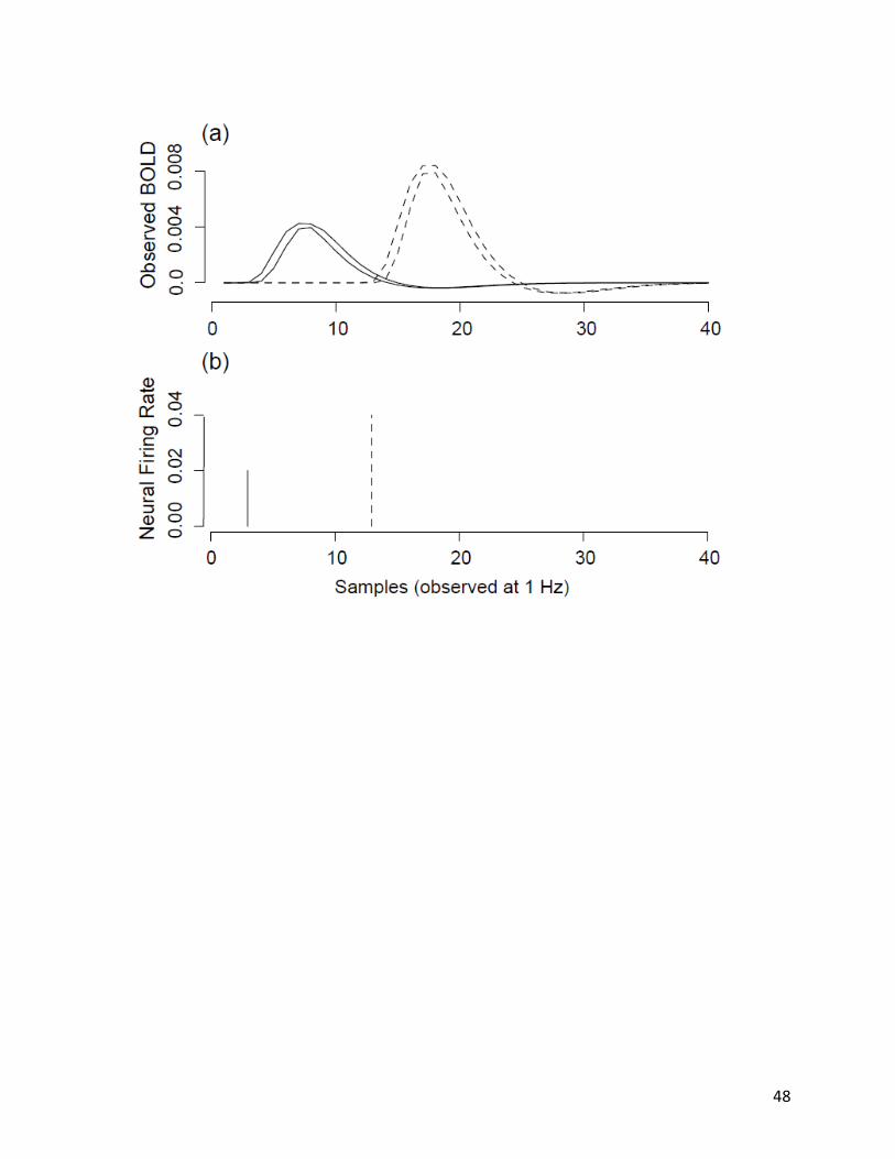
48

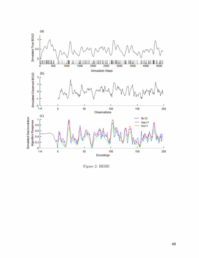
49

50

51

52

53

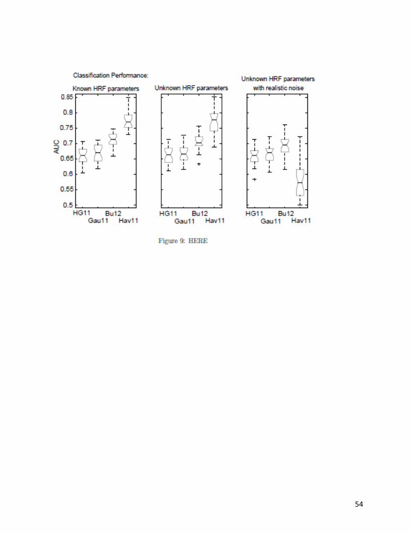
54