AN-Najah National UniversityFactuality of Engineering

Department of Electrical Engineering

Analysis ,Improvement,Conservation,and Design PV System For Electrical Network of the Beat Ommar Twon

Prepared by-: Iyad Obaid

Osama Yousef

Presented to-: Dr. Imad Ibrik

2010

Table of ContentsPageContentNO.

AcknowledgmentAbstractIntroductionElectrical networkChapter 1Electrical supply1.1Energy consumption1.2The nature of the load1.2.1The growth rate of the load1.2.2Daily load curve1.2.3Element of beat Ommar network1.3Distribution transformer1.3.1Medium voltage 33kv line1.3.2Analysis of the networkChapter 2ETAP power station2.1One line diagram2.2Data needed for the load flow analysis2.3The real and reactive power 2.3.1The length and the resistance2.3.2Load flow analysis2.4The medium voltage2.4.1Low tension voltage2.4.2Power factor2.4.3Load factor2.4.4Summary2.4.5Load flow analysis for minimum case2.5The medium voltage 2.5.1The low tension voltage2.5.2Summary2.5.3Problem of the network2.6Solution and recommendation2.7Electrical network improvementChapter 3Power factor improvement3.1problem of low power factor3.1.1How to improve the power factor 3.1.2

Distribution of the capacitor3.1.3The result of maximum case3.1.4Power factor after adding capacitor for max case3.1.4.1Summary of maximum case after correction3.1.4.2The result for minimum case 3.1.5Power factor after adding the capacitor for min case3.1.5.1Summary of min case after correction3.1.5.2Comparison between the original and improvement case 3.1.6Voltage correction 3.2Economy study3.3Energy conservationChapter 4Energy conservation for street lighting4.1Energy conservation for water pump4.2Energy conservation in residential sector4.3Replacing the incandescent lamp by the CFL lamp4.3.1Energy conservation for refrigerators4.3.2Load factor improvement4.4Design PV system for electrification of Safa villageChapter 5Introduction5.1The electrical loads of house hold for Safa village5.2Design of centralized PV system component for the Safa village 5.3PV generating sizing5.3.1The battery , charge regulator , and inverter5.3.2Electrical network map for centralized case5.3.3Design decentralized PV system component for Safa village 5.4PV generating sizing5.4.1The battery, charge regulator ,inverter5.4.2Economy evaluation of centralized and decentralized PV system for Safa village

5.5

The cost of centralized and decentralized PV system for Safa village5.5.1Which project we select centralized or decentralized5.5.2Cash flow for centralized PV system5.5.2.1Cash flow for decentralized PV system5.5.2.2Max overall efficiency for centralized and decentralized PV system5.6Building integrated photovoltaic (BIPV) system5.7

Acknowledgment

We would like to take the opportunity to thank people who guided and supported us

during this work.

We are very grateful to our parents whose have always given us their encouragement

and support.

We wish to express our deepest gratitude to our supervisor " Dr. Imad Ibrik " for

showing great interest in our work and for the guidance that he has given us.

Thanks to our doctors especially “Dr.prof.Marwan Mahmud” and “Dr.Maher

khammash” Head of Elec.Eng.Dep .

Thanks to our friends for their encouragement and mental support during this work.

Our thanks is also directed to everyone gives us information and help in our project,

especially the electrical department in BEAT OMMAR.

Abstract

Our project is to make a load flow study and analysis for BEAT OMMAR Electrical Network using ETAP software to improve the power factor and to reduce the electrical losses in the network and so, reducing the penalties in the total tariff for the municipality, increasing the reliability of the network. More over we want to increase the capability of the transformers and the transmission lines.

We made a conservation energy study in order to decrease the consumption and the peak demand. We made that study on all sectors of the network such as houses, street lighting, water pumping .. etc.

we made analysis for three houses on SAFA site, and design of centralized and decentralized PV system component for these houses and we made economic model for selection optimum configuration of PV system (centralized and decentralized ).

To do that we will follow the sequence bellow :

Analyzing this network by collecting data such as resistance and reactance, length, rated voltages, max power and reactive power on each bus .

We entered these data to the software ( ETAP) and getting the results .

We will give recommendations and conclusions.

The improvements for elements of the network.

Study the three houses load.

Design of centralized and decentralized PV system for these houses.

Introduction

The power system in general consists of these parts:

1) Generating station: And this part consists of

i) Generators in which electric power is produced by 3-phase alternators operating in parallel. And usually electric power is generated at voltages of 12kv to 25kv.

ii) Sub-station, where the power transformers step up the voltage to between 66kv 1000kv.

2) Primary transmission. The electric power at high voltages is transmitted by 3-phase 3-wire over head system to the outskirts of the city. This forms the primary transmission.

3) Secondary transmission. The primary transmission line terminates at the receiving station which usually lies at the outskirts of the city. At the receiving station the voltage is reduced to 33kv or 22kv by step-down transformers. From this station, electric power is transmitted at one of these voltages by 3-phase 3-wire overhead system to various sub-stations located at strategic points in the city. This forms the secondary transmission.

4) Primary distribution. the secondary transmission line terminates at the sub-station where voltage is reduced from the secondary voltage to the primary distribution voltage usually 11kv ,could be 6.6kv 3-phase 3-wire .the 11kv lines run along the important road sides of the city . And forms the primary distribution.

5) Secondary distribution. The electric power form primary distribution line is delivered to distribution sub-stations. These sub-stations are located near the consumers localities and step down the voltage to 400v 3-phase 4-wire for secondary distribution. And this forms secondary distribution.

Energy sector in Palestine

Energy sector in Palestine faced sever since the Israeli occupation , financial and management obstacles due to the severe restrictions imposed by the Israeli occupation. as a result of this situation Palestine has not yet a unified power system , the existing network is local low voltage distributions networks connected to Israeli electrical corporation (IEC) , where around 97% of consumed energy were and still supplied by the IEC .

The voltages of the existing distribution networks are : ( 0.4 , 6.6 , 11 , 22 , and 33 KV ) . IEC supplies electricity to the electrified communities by 22 or 33 KV by overhead lines . electricity is purchased from IEC and then distributed to the consumers.

The existing electricity situation is characterized in old fashion over loaded networks , high power losses ( more than 20% ) , low power factor ,poor system reliability , high prices of electricity supplied to the consumer due to high tariff determined by the IEC in addition , many villages depend on diesel generators to provide their own needs of electrical energy .

Due to all factors mentioned above, it becomes very important to design a national independent power system for the west bank of Palestine which will connect all the west bank areas by a reliable network to a national generating plant . the national power system should have the minimum annual cost and provide the consumer with a high quality of electric energy . this power system should also reduced the cost of KWH and be able to provide electricity to any area in the west bank .

Load flow analysis

In power system analysis The Load Flow study is a basic and commonly needed electrical study. The Load Flow study will show the power in KVA or Amperes that is being handled by all of the individual electrical components, e.g. transformers, conductors and panels in the system. This allows a determination of equipment rating margins and reserve capacity loading percentage.

Analysis and study of distribution electrical networks may cover conventional voltage drop analysis, power losses analysis, power factor considerations, capacitors’ placements (correction of power factor).

Prospective goals of the study :-

1. Reduction of power losses2. Increasing of voltage levels

3. Reducing the penalties by improving the P.F. 4. Increasing the capability of the transformers. 5. Increasing the reliability of the network .

Methods of improvement of operating condition in electrical networks :-

1. Swing bus control2. Transformer taps3. Installation of capacitor banks (reactive power compensation) 4. Changing the configuration of distribution network (radial ring)

Power factor improvement

The cosine of angle of Phase displacement between voltage and current in an AC circuit is known as Power Factor. The Reactive component is a measure of the Power Factor.

Under normal operating conditions certain electrical loads (e.g. induction motors, welding equipment, arc furnaces and fluorescent lighting (draw not only active power from the supply (kilowatts, kW) but also reactive power (reactive KVAR). This reactive power is necessary for the equipment to operate correctly but could be interpreted as an undesirable burden on the supply.

Capacitor banks

The important method of improvement power factor is by adding shunt capacitor banks at the buses at both transmission and distribution levels and loads and there are more effective to add them in the low level voltages.

Effect of Low Power Factor

Higher Apparent Current Higher Losses in the Electrical Distribution network Low Voltage in the network

Benefits of Improving Power Factor

Lower Apparent Power. Reduces losses in the transmission line . Improves voltage drop. Reduces load factor on transformers. Avoiding the penalties.

Information about Beat Ommar town :

Beat Ommar Palestinian town located in the north of the city of Hebron, the distance between Beat Ommar and the city is about 11 km. Beat Ommar rise 765 meters above sea level and covers an area of land (30129) dunum , Beat Ommar has a population of about 23000 people .

Khirbat Safa is located northwest of the town of Beat Ommar of the town, which suffers from the problem of roads, and electricity.

Surrounding the town of Beat Ommar from all sides of many of the colonies as a colony and the colony of Bat Ayin Gush Etzion.

Chapter One

1.1 Electrical Supply

Beat Ommar distribution network is supplied by the IEC ( Israel electrical company ) directly, there is only one connection point at Safa through an overhead lines of 33kv . the main circuit breaker is rated at 129A . the max demand is reached 5.391 MVA.

We have the only connection point in the town Safa . The IEC supplies the network with 108A, which is very little value comparing with the needs of the consumers, for example; the maximum demand reach the value of 108A in the summer which exposes the network to the danger and the cutoff of supply. so we have to demand ( purchase) another 60A from the IEC to

cover the needs of Beat Ommar from electricity and put the network in the Safe side and increase the reliability of the network.

1.2 Energy Consumption :

In this section we will talk about the consumption of energy in Beat Ommar network.

1.2.1 The Nature Of The Load.

The table bellow shows the consumers classification and their size.

Type of load Consumption %

Residential 62%

Industrial 11%

Commercial 13%

Water pumps+ light 14%

We see that the biggest consumer is the residential sector which achieve about 62 % from the total consumption, also the water pump and street lighting sector has a high percentage from the total consumption. There are many factories in Beat Ommar that consume a big amount of power.

1.2.2 The growth rate of the load

The table below shows the total consumption of energy for 4 years .

Year Average Monthly consumption

In MWH

Percentage growth %

2006 646 ---------------

2007 717 10.99%

2008 797 11.15%

2009 880 10.41%

We notice that the energy purchased from the ICE is changing during theYears.

A jump in the power consumption happened in 2008 by nearly 80 MWH.

And here is the monthly energy consumption in MWH in the last 4 years

2009 2008 2007 2006

month P (MWH) month P

(MWH) month P (MWH) month P

(MWH)1 875.1 1 790.3 1 710.3 1 640.1

2 865.9 2 788.7 2 708.3 2 637.9

3 861.3 3 781.9 3 703.1 3 630.2

4 873.6 4 777.8 4 701.5 4 619.5

5 875.2 5 771.9 5 699.6 5 611.1

6 869.4 6 762.7 6 697.7 6 607.3

7 881.6 7 774.1 7 692.1 7 599.8

8 890.6 8 800.1 8 725.5 8 600.2

9 880.1 9 797 9 716.3 9 643.3

10 882.3 10 793.3 10 709.2 10 660.2

11 876.3 11 789 11 701.6 11 629.7

12 872.1 12 785.2 12 699.6 12 622.7

TOTAL = 10560 MWH TOTAL = 9564 MWH TOTAL = 8604.8 MWH TOTAL = 7752 MWH

Note: We note that the peak power is occurs in August and October .

In graphical mode :

1.2.3 Daily load curve

We take readings to the load changes during the day, the result gives the graph below :

Note : that readings were taken in September 2009

From the above graph we notice the following :

The maximum power consumed 5.463 MW and occurred at 1:45 pm . The peak demand occurs at two intervals :

1. 10:30 am – 03:15 pm 2. 07:30 pm – 10:00 pm

The average demand is about 4.1 MW

1.3 Elements Of Beat Ommar Network

In this section we will study the elements of the network such as transformers, over head lines and underground cables.

1.3.1 Distribution Transformers:

Beat Ommar network consists of 26 - Δ/Υ - , 33/0.4 KV distribution transformers.

And the table shows the number of each of them and the rated KVA.

Number of Transformers

Transformer Ratings (KVA)

11 630

9 400

6 250

1.3.2 Medium voltage 33kv lines :

1. Overhead lines

The conductors used in the network are ACSR (50mm2) , and their Resistance R=(0.543/Km) and Reactance X= (0.297 /Km) ,

2. Underground cables

The Underground cables used in the network are XLPE Cu (120 mm2) and their Resistance R= (0.303 /Km) and Reactance X= (0.27 /Km)

Chapter Two

Analysis Of The Network

2.1 ETAP power station :-

ETAP PowerStation allows us to work directly with graphical one line diagram.And it provides us with text reports such as: complete report. Input data. Results . Summary reports

2.2 One line diagram

In order to have the one line diagram, we followed the network diagram from the network plans , and so we get this plan considered as an input to the ETAP program .

2.3 Data needed for the load flow analysis.

2.3.1 The real and reactive power

( OR apparent power and P.F OR Ampere and P.F ).

And the given table gives the real and reactive power on each bus.

Number of bus P (kw) Q (kvar)1 5.463 2.8962 0.295 0.1433 0.580 0.3234 0.483 0.2715 0.280 0.1706 0.278 0.1587 0.201 0.0928 0.096 0.0499 4.584 2.416

10 4.583 2.41511 0.185 0.10212 0.184 0.09414 4.327 2.27615 3.844 2.03016 0.118 0.05417 0.477 0.24318 0.248 0.12019 0.227 0.11420 0.277 0.11421 0.225 0.10322 3.725 1.97123 0.076 0.03724 3.640 1.92725 0.139 0.07926 0.138 0.07527 3.498 1.84728 0.512 0.26029 0.196 0.09530 0.314 0.15631 0.312 0.14232 2.985 1.58533 0.055 0.04134 0.185 0.09735 0.185 0.09736 0.185 0.09737 0.183 0.089

38 2.743 1.44539 0.184 0.08940 2.554 1.34641 0.267 0.12942 2.282 1.20443 0.301 0.14644 0.291 0.14945 1.685 0.88346 0.173 0.07947 0.934 0.49548 0.436 0.23349 0.132 0.06850 0.300 0.14551 0.499 0.26252 0.195 0.09453 0.302 0.15954 0.300 0.14555 0.577 0.30256 0.283 0.13757 0.291 0.15258 0.289 0.14059 0.070 0.034

2.3.2 The length and Resistances

R in (Ω) and X in (Ω) of the lines.

After formatting the one line diagram of the network, and dividing it into buses we formed this table which shows the length of the lines and their resistance and reactance.

Cables and Lines Length (m) Resistance (Ω) Reactance (Ω)Cable 1 110 0.0333 0.0312Cable 2 105 0.3180 0.0311Cable 3 100 0.3030 0.0270Cable 4 100 0.3030 0.0270Cable 5 100 0.3030 0.0270Line 1 100 0.0543 0.0297Line 2 90 0.0488 0.0267Line 3 100 0.0543 0.0297Line 4 210 0.1140 0.0623Line 5 650 0.3529 0.1930Line 6 610 0.3312 0.1811Line 7 110 0.0597 0.0326Line 8 200 0.1086 0.0594Line 9 320 0.1737 0.0950Line 10 1000 0.5430 0.2970Line 11 310 0.1683 0.0920Line 12 220 0.1194 0.0653Line 13 190 0.1031 0.0564Line 14 110 0.0597 0.0326Line 15 210 0.1140 0.0623Line 16 310 0.1683 0.0920Line 17 850 0.4615 0.2524Line 18 100 0.0543 0.0297Line 19 900 0.4887 0.2673Line 20 900 0.4887 0.2673Line 21 100 0.0543 0.0297Line 22 220 0.1194 0.0653Line 23 100 0.5430 0.0297Line 24 200 0.1086 0.0594Line 25 120 0.0650 0.0356Line 26 100 0.0543 0.0297

.

2.4 load flow analysis for max case

2.4.1 the medium voltages

The actual medium voltages on each transformer is shown in the table below :

Transformernumber

Medium voltage(rated)kv

Medium voltage(actual)kv

T1 33 33T2 33 32.99T3 33 32.99T4 33 32.997T5 33 32.97T6 33 32.973T7 33 32.917T8 33 32.965T9 33 32.96T10 33 32.908T11 33 32.83T12 33 32.806T13 33 32.805T14 33 32.795T15 33 32.791T16 33 32.777T17 33 32.728T18 33 32.684T19 33 32.684T20 33 32.68T21 33 32.674T22 33 32.674T23 33 32.675T24 33 32.674T25 33 32.679T26 33 32.679

Note : the colored values refers to the least medium voltages which has more drop of voltages.

2.4.2 The low tension voltages

The actual low voltages on each transformer is shown in the table below :

Transformernumber

Low voltage(rated)kv

Low voltage(actual)v

T1 0.4 391T2 0.4 392T3 0.4 392T4 0.4 39T5 0.4 39T6 0.4 394T7 0.4 39T8 0.4 392T9 0.4 389

T10 0.4 393T11 0.4 391T12 0.4 388T13 0.4 388T14 0.4 392T15 0.4 388T16 0.4 388T17 0.4 388T18 0.4 387T19 0.4 387T20 0.4 388T21 0.4 387T22 0.4 385T23 0.4 386T24 0.4 387T25 0.4 387T26 0.4 387

Note : the colored values refers to the least low voltages which has more drop of voltages.

2.4.3 Power factorThe table below shows the power factor, real and reactive power on each transformer:

No .of transformer P (KW) Q (KVAR) P.F %

T1 295 143 90T2 96 49 89T3 201 92 91T4 278 158 87T5 184 94 89T6 70 34 90T7 118 54 91T8 248 120 90T9 225 103 91T10 76 37 90T11 138 75 88T12 196 95 90T13 312 142 91T14 55 41 80T15 183 89 90T16 184 89 90T17 267 129 90T18 301 146 90T19 391 149 89T20 173 79 91T21 300 145 90T22 132 68 90T23 195 94 90T24 300 145 90T25 283 137 90T26 289 140 90

Note : the power factor reach between 0.91 and 0.87 . This causes more penalties on the total bill

2.4.4 Load factor

The load factor is known as the average power divided by the rated power.

No .of transformer T. ratings (KVA) T. load(KVA) Load factor %

T1 630 343 54.4

T2 250 112 44.8T3 400 232 58T4 630 336 53.3T5 400 217 54.2T6 250 80 32T7 250 136 54.4T8 630 287 45.5T9 400 262 65.5

T10 250 87 34.8T11 400 165 41.2T12 400 232 58T13 630 364 57.7T14 250 72 28.8T15 400 216 54T16 400 217 54.2T17 630 315 50T18 630 358 56.8T19 630 350 55.5T20 400 202 50.5T21 630 357 56.6T22 250 160 64T23 400 232 58T24 630 357 56.6T25 630 336 53.3T26 630 343 54.4

L.F Somewhere reaches 65.5% , and it drops to 32% in other buses .

There is no over loaded transformers in the network, but some of the transformers is under loaded .

2.4.5 Summery

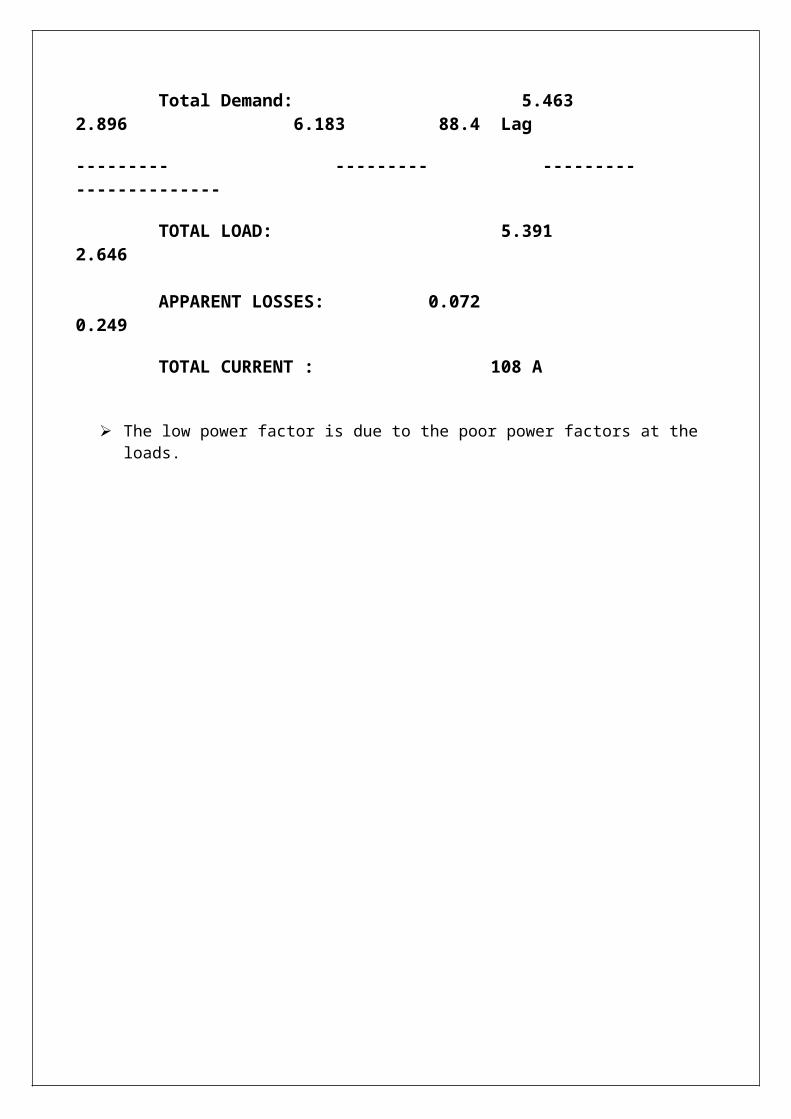
we have to summarize the results, total generation, demand , loading., percentage of losses, and the total power factor for the maximum case.

MW MVAR MVA % PF ========= ========= ========= ===== =======

SWING BUS: 5.463 2.896 6.183 88.4 Lag Total Demand: 5.463 2.896 6.183 88.4 Lag --------- --------- --------- -------------- TOTAL LOAD: 5.391 2.646 APPARENT LOSSES: 0.072 0.249 TOTAL CURRENT : 108 A

The low power factor is due to the poor power factors at the loads.

2.5 load flow analysis for min case

2.5.1 the medium voltages

The actual medium voltages on each transformer is shown in the table below :

Transformernumber

Medium voltage(rated)kv

Medium voltage(actual)kv

T1 33 33T2 33 32.999

T3 33 32.999T4 33 32.999T5 33 32.985T6 33 32.986T7 33 32.958T8 33 32.982T9 33 32.98T10 33 32.953T11 33 32.913T12 33 32.901T13 33 32.901T14 33 32.896T15 33 32.894T16 33 32.887T17 33 32.862T18 33 32.839T19 33 32.839T20 33 32.837T21 33 32.834T22 33 32.834T23 33 32.835T24 33 32.835T25 33 32.837T26 33 32.837

.

2.5.2 The low tension voltages

The actual low voltages on each transformer is shown in the table below :

Transformernumber

Low voltage(rated)kv

Low voltage(actual)v

T1 0.4 395T2 0.4 395T3 0.4 395T4 0.4 395T5 0.4 395T6 0.4 397T7 0.4 395

T8 0.4 396T9 0.4 394

T10 0.4 396T11 0.4 395T12 0.4 394T13 0.4 394T14 0.4 396T15 0.4 394T16 0.4 394T17 0.4 394T18 0.4 393T19 0.4 393T20 0.4 394T21 0.4 393T22 0.4 392T23 0.4 393T24 0.4 393T25 0.4 394T26 0.4 393

2.5.3 Summery

we have to summarize the results, total generation, demand , loading., percentage of losses, and the total power factor for the maximum case.

MW MVAR MVA % PF ========= ========= ========= ===== ======= SWING BUS: 2.807 1.433 3.151 89.1 Lagging TOTAL DEMAND: 2.807 1.433 3.151 89.1 Lagging

--------- --------- --------- --------------

TOTAL LOAD: 2.788 1.369

APPARENT LOSSES: 0.019 0.065 TOTAL CURRENT : 55 A

The min load is equal to 50% of the max load

2.6 Problems Of The Network

We can summarize the general problems of the network by the following points :

The consumed power is reached the maximum limit , which causes over load currents . This result in disconnecting the supply of the town .

The P.F is less than 0.92 ; this cause penalties and power losses.

There is a voltage drop and power losses

2.7 Solutions And Recommendations

Increasing the supply from the IEC from the main circuit breaker .

Using capacitor banks to improve the P.F and so, reducing the power losses , and avoiding the penalties.

Managing the max peak demand by :

1. shift of max demand. 2. using other sources.

Conservation of energy .

Increasing the reliability of the system by developing another configurations ( Ring off ) .

Using PV modules

Chapter Three

Electrical Network Improvements

3.1 Power factor improvement

3.1.1 The problem of low power factor

The low P.F is highly undesirable as it causes an increase in current, resulting in additional losses of active power in all the elements of power system from power station generator down to the utilization devices.

In addition to the losses the low P.F causes penalties, for example for every 1% P.F below 92% and above 80% costs us 1% of the total bill.

3.1.2 How to improve the P.F

Where: Qc: the reactive power to be compensated by

the capacitor. P: the real power of the load. Ø old: the actual power angle. Ø New: the proposed power angle.

COMPENSATION AT L.V. IS PROVIDED BY

1- Fixed values of capacitors. 2- Automatic capacitor banks.

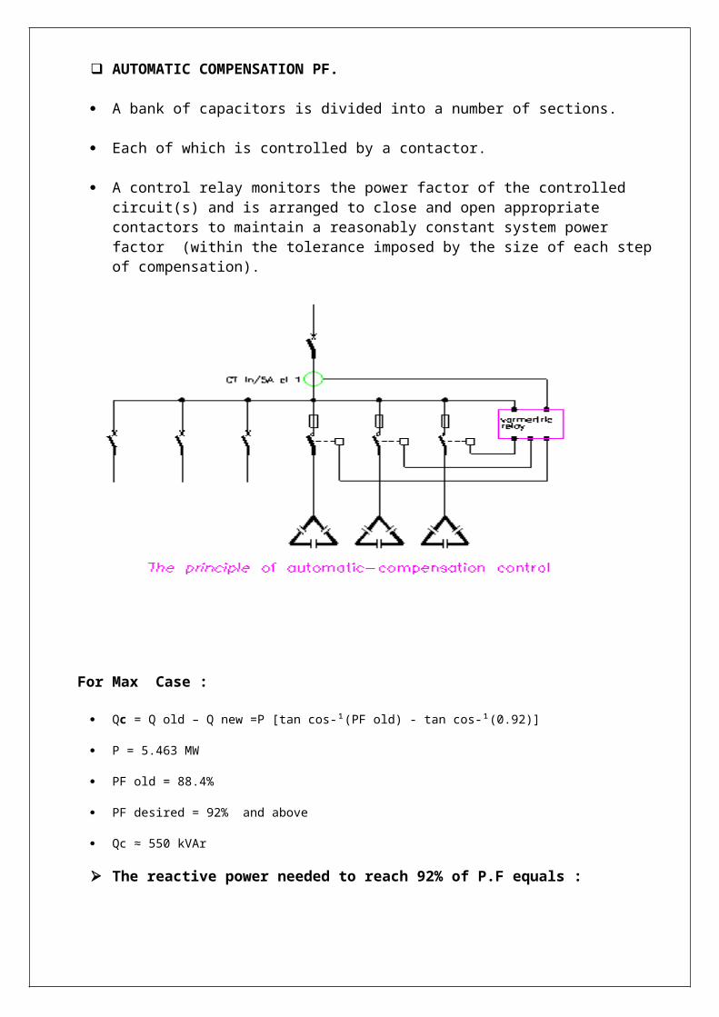
AUTOMATIC COMPENSATION PF.

A bank of capacitors is divided into a number of sections.

Each of which is controlled by a contactor.

A control relay monitors the power factor of the controlled circuit(s) and is arranged to close and open appropriate contactors to maintain a reasonably constant system power factor (within the tolerance imposed by the size of each step of compensation).

For Max Case :

Qc = Q old – Q new =P [tan cos-¹(PF old) - tan cos-¹(0.92)]

P = 5.463 MW

PF old = 88.4%

PF desired = 92% and above

Qc ≈ 550 kVAr

The reactive power needed to reach 92% of P.F equals :

Qc ≈ 550 kVAr

** Which will cause the P.F in the min case to be 95.2% lag.

3.1.3 The distribution of capacitors

The following table shows the distribution of the capacitor banks and its effect on the P.F on each transformer.

#of Transformers

Qc (kvar) Old P.F% Max case New P.F %

Min case New P.F %

1 30 90 92.1 95.62 10 89 91.4 94.14 60 87 93 985 30 89 93.1 97.76 10 90 93.9 97.78 30 90 92.9 96.6

10 10 90 93.5 97.211 25 88 93 97.912 25 90 92.7 96.7

14 20 80 92.9 9815 20 90 92.3 95.916 20 90 92.2 95.417 30 90 92.4 9618 30 90 91.9 95.319 40 89 91.9 96.521 30 90 91.9 95.322 20 89 92.4 9723 20 90 91.9 95.524 30 90 91.9 95.325 30 90 92.1 95.726 30 90 92.1 95.6

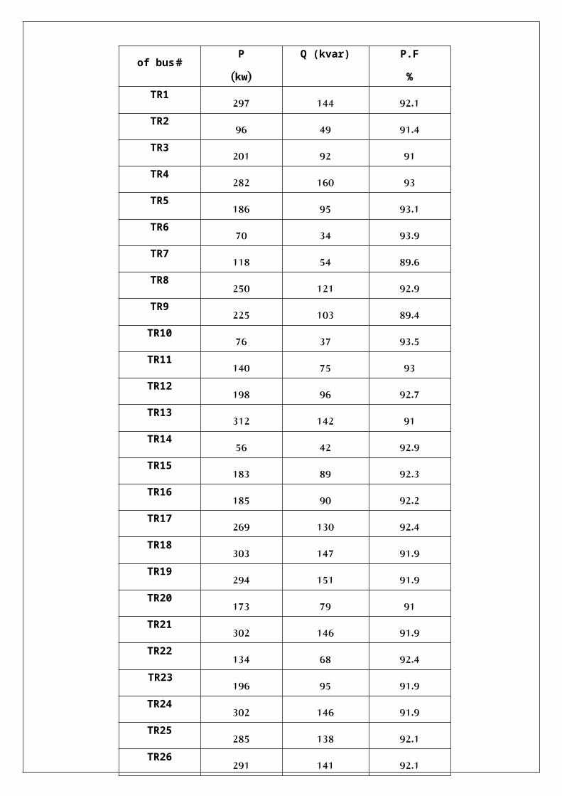
3.1.4 The results for max case

3.1.4.1 Power factor after adding capacitors for max case

3.1.4.2 Summary of max case after correction

we can summarize the results, total generation, demand , loading., percentage of losses, and the total power factor for the maximum case.

#of bus P)kw(

Q (kvar) P.F%

TR1 297 144 92.1TR2 96 49 91.4TR3 201 92 91TR4 282 160 93TR5 186 95 93.1TR6 70 34 93.9TR7 118 54 89.6TR8 250 121 92.9TR9 225 103 89.4

TR10 76 37 93.5TR11 140 75 93TR12 198 96 92.7TR13 312 142 91TR14 56 42 92.9TR15 183 89 92.3TR16 185 90 92.2TR17 269 130 92.4TR18 303 147 91.9TR19 294 151 91.9TR20 173 79 91TR21 302 146 91.9TR22 134 68 92.4TR23 196 95 91.9TR24 302 146 91.9TR25 285 138 92.1TR26 291 141 92.1

MW Mvar MVA % PF ===== ===== ===== ======

Swing Bus: 5.494 2.374 5.985 91.8 Lagging

Total Demand: 5.494 2.374 5.985 91.8 Lagging --------- --------- --------- --------------

Total Load: 5.426 2.139

Apparent Losses: 0.068 0.235

Total current 105A. ( Before the capacitors the total current was 108A ).

Saving in the real power P = 4 KW.

Saving in the reactive power Q = 14 Kvar.

3.1.5 The results for min case

3.1.5.1 Power factor after adding capacitors for min case

3.1.5.2 Summary of min case after correction

#of bus P)kw(

Q (kvar) P.F%

TR1 152 74 95.6TR2 58 30 94.1TR3 103 47 91TR4 145 82 98.5TR5 96 49 97.7TR6 36 17 97.7TR7 60 28 91TR8 128 62 96.6TR9 116 53 90.2

TR10 39 19 97.2TR11 72 39 97.9TR12 102 49 96.7TR13 161 73 91TR14 29 21 98TR15 94 46 95.9TR16 96 46 95.4TR17 139 67 96TR18 157 76 95.3TR19 152 78 96.5TR20 89 41 91TR21 157 76 95.3TR22 69 36 97TR23 102 49 95.5TR24 157 76 95.3TR25 147 71 95.7TR26 151 73 95.6

we can summarize the results, total generation, demand , loading., percentage of losses, and the total power factor for the maximum case.

MW Mvar MVA % PF ===== ======= ======= =======

Swing Bus: 2.823 0.896 2.962 95.3 Lagging

Total Demand: 2.823 0.896 2.962 95.3 Lagging --------- --------- --------- -------------- Total Load: 2.806 0.838

Apparent Losses: 0.017 0.058

Total current 52A. ( Before the capacitors the total current was 55A ).

Saving in the real power P = 2 KW.

Saving in the reactive power Q = 7 Kvar.

3.1.6 Comparison between the original and improved cases

Original case After improvement PF

3.2 Voltage correction

The table bellow shows the voltage ranges before and after adding capacitor banks for the two levels of voltage.

#of Transforme

r

Medium voltage

Kv before

Medium voltage

Kv after

Low voltage

Kv before

Low voltage

Kv after

TR1 33 33 0.391 0.392TR2 32.99 32.999 0.392 0.393TR3 32.99 32.99 0.392 0.390TR4 32.997 32.997 0.39 0.393TR5 32.97 32.971 0.39 0.392TR6 32.973 32.974 0.394 0.395TR7 32.917 32.92 0.39 0.390TR8 32.965 32.966 0.392 0.393TR9 32.96 32.961 0.389 0.389

TR10 32.908 93.912 0.393 0.394TR11 32.83 93.836 0.391 0.392TR12 32.806 32.813 0.388 0.393TR13 32.805 32.812 0.388 0.388TR14 32.795 32.803 0.392 0.394TR15 32.791 32.799 0.388 0.389TR16 32.777 32.785 0.388 0.390TR17 32.728 32.738 0.388 0.390TR18 32.684 32.695 0.387 0.388TR19 32.684 32.695 0.387 0.388TR20 32.68 32.692 0.388 0.388TR21 32.674 32.686 0.387 0.388TR22 32.674 32.686 0.385 0.387TR23 32.675 32.686 0.386 0.388TR24 32.674 32.686 0.387 0.388TR25 32.679 32.691 0.387 0.389TR26 32.679 32.69 0.387 0.388

3.2 Economical study

In order to make sure that adding the capacitor banks, we should make an economical study to see if that is feasible .

So we have to know how much saving in power and energy we have, also we have to calculate the simple payback period ( S.P.B.P ) which known as the investment of money through capacitors divided by the total saving in energy through a year.

Simple payback period

0.8≤PF<0.92 penalties is 1% of the total bill for every 0.01 of P.F. < 0.92 0.7≤PF<0.8 penalties is 1.25 % of the total bill for every 0.01 of P.F < 0.8

PF< 0.7 penalties is 1.5% of the total bill for every 0.01 of P.F < 0.7

Average monthly consumption = 880000 kwh

Total bill (NIS/year) = 880000kwh * 12 month * 0.5(NIS/kwh)=5280000 NIS/year

Saving in penalties = (91.8-88.4) * 1% * 5280000 NIS/year

Saving in penalties = 179520 NIS/year

Saving in energy = ∆P * τ* (NIS/kwh)) = 0.072-0.0680(KW *2500h*(0.5)

Saving in energy = 5500 NIS/year

Saving per year = saving in penalties + saving in energy = 179520 + 5500

Saving per year = 185020 NIS/year

Capital cost = cost of capacitors =Q(KVAR) * (15 JD/KVAR) * 6 NIS = 550 * 15* 6

Capital cost = 49500 NIS

S.P.B.P = capital cost / (saving per year)

= 49500 / 185020

S.P.B.P = 0.2675 year = 3.21 month = 96 day

Note : since the S.P.B.P less than two years then the project is feasible.

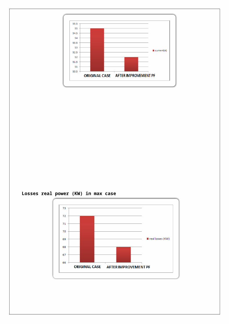
Current in max case

Current in min case

Losses real power (KW) in max case

Losses real power(KW) in min case

Power factor in max case

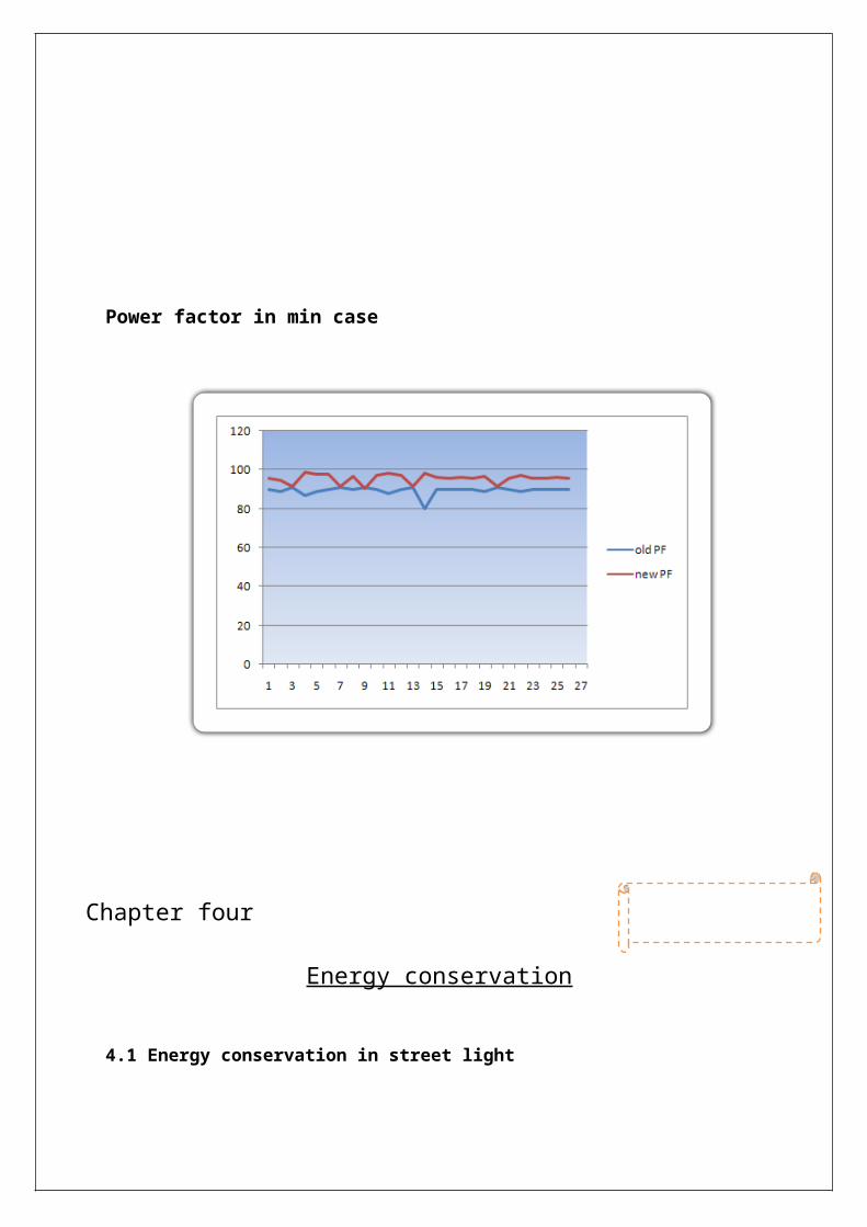
Power factor in min case

Chapter four

Energy conservation

4.1 Energy conservation in street light

In Beat Ommar town we have a number of street lamps ( about 1100 ) lamps distributed in the streets with rated power of 125 w for 500 lamps, and 70 w for 600 lamps .

We have to conserve energy in this sector by replacing the 125 w lamps by the 70 w lamps .

#of street lamps

Power (W) After replacement

Saving energy(KWH)/year

Saving in cost NIS/ year

600 70 70 0 0

500 125 70 120450 66247

Then we should show the saving in power and energy and money. Also the simple payback period to recover the cost is very important .

Calculations :

ΔP=(125-70)=55W, for each lamp.

Working hours per day=12 Hr, and 4380 Hr per year

Saving energy per year = ΔP *#of lamps*hrs per year. =55*500*4380/1000= 120450(Kwh)/year.

Cost of energy =0.55 NIS/Kwh.

Saving in cost=0.55*120450= 66247 NIS./year.

Cost of each lamp=250NIS and for all lamps = 125000 NIS.

S.P.B.P=capital cost/saving per ye =125000NIS/66247(NIS/year).=1.8year

=1.8*12=22.64 months

Note : since the S.P.B.P less than 5 years then the project is feasible.

4.2 Energy conservation in water pumps

In Beat Ommar we have 9 water pumps, 3 of them are operating by using diesel fuel.

The other 6 motors are working by electricity. We can save energy in this sector by replacing the less efficient ones by another motors of high efficiency as follows :

Existing motors

#of motor Output power(KW)

Efficiency% Input power(KW)

ΔP(KW) Working hours

Working time

4 55 90 61.1 6.1 18 5 am to 11 pm

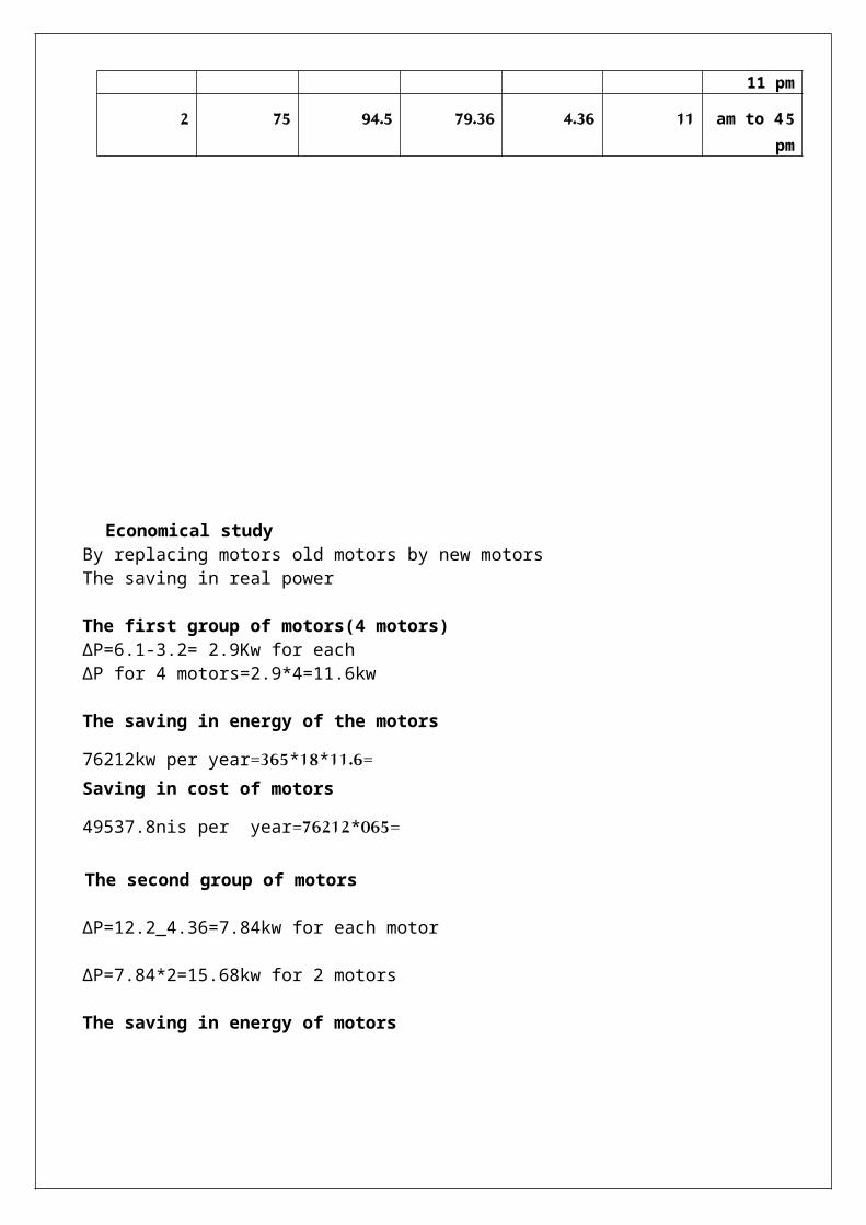
2 75 86 87.2 12.2 11 5 am to 4 pm

New motors

#of motor Output power(KW)

Efficiency% Input power(KW)

ΔP(KW) Working hours

Working time

4 55 94.4 58.2 3.2 18 5 am to 11 pm

2 75 94.5 79.36 4.36 11 5 am to 4 pm

Economical study By replacing motors old motors by new motors

The saving in real power

The first group of motors(4 motors) ΔP=6.1-3.2= 2.9Kw for each

ΔP for 4 motors=2.9*4=11.6kw

The saving in energy of the motors=11.6*18*365=76212kw per year

Saving in cost of motors=065*76212=49537.8nis per year

The second group of motors

ΔP=12.2_4.36=7.84kw for each motor

ΔP=7.84*2=15.68kw for 2 motors

The saving in energy of motors

=15.68kw*11hr*365=62955.2 kw per year

The saving in cost of motors

=0.65*62955.2=40920.88nis per year

The cost of 75 hp motor and Efficiency =94.4 is 5000 $

Corresponds to 20000 NIS

The cost of 100hp motor and Efficiency =94.4 is 6000 $

corresponds to 24000 NIS

The total cost of 4 motors (75hp) =80000 NIS The total cost of 2 motors (100hp) =48000 NIS

The first group of motors (75hp)

S.P.B.P =80000/49537.8=1.61 year =19 month

The second group of motors (100hp)

S.P.B.P =48000/40920.8=1.17 year=14 month

Note: we can Manage the max peak demand by shifting the operating time of the first two motors in group 1 and all the motors in group 2, which works on the peak time. 7:30 pm to 10:00 pm From the daily load curve

4.3 Energy conservation in residential sector.

4.3.1 Replacing the incandescent lamps by the CFL lamps.

Note: we have 2400 consumers.

Inc.lamp75w CFL lamp15w

Price(NIS) 1.5 25

Life time (hours) 1000 10000

Cost over life time(NIS) 10*1.5=15 25*1=25

Kwh in 10000 hr 750 150

Energy cost in 10000 hr

(NIS)

0.65*750=487.5 0.65*150=97.5

Total cost(NIS) 487.5+15=502.5 25+97.5=122.5

Saving in 10000 hr 502.5-122.5=380 (NIS)

We notice that we can save 380(NIS) by using the CFL lamps during the operating life for one lamp .

Economy study

Each home have about 5 lamps in average, and it work about 5 hours per day

Total lamps = 2400*5=12000 lamps.

Energy consumption per year ( Inc 75 W)= 75 *12000*5*365 =1642500 Kwh/year.

Energy consumption per year ( CFL15 W)= 15*12000*5*365=328500 Kwh/year.

Saving in energy = 1314000Kwh/year.

Saving in cost = 1314000 * 0.65 = 854100 NIS/ year.

Fixed cost/year = (8760/10000)*25*12000 = 262800 NIS

S.P.B.P = 262800 NIS /854100 (NIS/year) = 0.307year= 3.69 months.

S.P.B.P for each consumer

We see that the replacement is feasible and the consumer save 356 NIS per year.

Total lamps = 5 lamps.

Energy consumption per year ( Inc 75 W)

= 75*5*365*5 =684.375 Kwh/year.

Energy consumption per year ( CFL15 W)

=15*5*365*5= 136.875Kwh/year.

Saving in energy =548Kwh/year.

Saving in cost = 584* 0.65 = 356.2NIS/ year.

Fixed cost/year = (8760/10000)*25*5 = 109.5NIS

S.P.B.P = 109.5NIS /356.2(NIS/year) = 0.307 year

= 3.6months.

4.3.2 Energy conservation in refrigerators:

In this section of energy conservation in the residential sector we aim to replace the old refrigerators which consumes high energy by new refrigerators which consumes less power energy than the old one. And we will make the feasibility study using the simple payback period (S.P.B.P) method.

In beat ommar village 2600 refrigerators at least1000 of its is old .if we replace it by new type

We notice the following

The table below shows the old refrigerators and their size and their consumption in Kwh/day . And the new refrigerators to be replaced by.

Type of refrigerator

Size in(Ltr)

KWh/day Cost (NIS)

Type of new one

KWh/day Cost (NIS)

amcor 430 2.9 1200 LG 1.2 3000

Life cycle for Amcor =5 years

Life Cycle for LG =10years

Annual fixed cost for amcor =1200/5=240 NIS

Annual fixed cost for LG =3000/10=300 NIS

Running cost /year for amcor =2.9*365.*65=688NIS

Running cost for LG =1.2*365*.65=284NIS

Total cost /year =240+688 =928 NIS for amcor

Total cost /year =300+284 =584 NIS for LGSaving money /year =928_584=344NISDifference in cost =3000_1200=1800NISS.P.B.P= 1800/344=5.2 years

4.4 Load factor improvement:

The load factor equal the average power divided by the maximum power, and so it is less than one and the best load factor which is equal to unity, and to do this we have to reduce the maximum demand as possible to be equal the average power.

From the daily load curve , we see that the average demand is 4.1 MW.

and the maximum peak demand is 5.463 MW.

The total load factor = Pav/ Pmax = 72%.

To improve the load factor and reducing the peak demand we suggest some notes :

1. shifting some of loads operating at the max point. The water pumps which operate through the duration of max load should work at another time .

2. adding capacitors in the transformers decreases the losses and the apparent power and so the peak demand .

Chapter Five

design of PV system for electrification of Safa Villiage

5.1 Introduction

The main characteristics of using PV system for electrification ofsmall rural villages are: the fuel is free, technology is mature and almostworldwide available and it has modularity, low maintenance requirements,high durability and also they can easily be connected to the utility network.A rooftop mounted decentralized photovoltaic system is one of theapplications of solar PV systems that has attracted lots of interest amongthe people in our region. The generation of electricity by this system isattractive because :* Generation is one-site. This results in reduction of transmission anddistribution costs and losses;* The cost of roofing tiles can be eliminated by using mounted PV systemsinstead;* There is no need for additional land for power generationThe only factor hindering the growth of utilization of PVdecentralized systems is relatively high capital cost.Another configuration that photovoltaic can have a majorcontribution is in centralized generating electricity for people living inisolated areas. Developing a method based on life cycle cost to select theoptimum configuration (centralized or decentralized ) will help inincreasing the utilization of PV systems

information about Safa village

Safa site is a small village that located north west of the town of Beat Ommar and away from it 4.5 km, which suffers from the problem of roads ,and electricity.

the houses lunch power from diesel generator ( 5KW, engine 9HP , fuel capacity 8 Gallons , run time at 50% load is 18 HR , number of hour operation is 14 HR as 8-12AM , 2-12 PM )

5.2 The electrical loads of household for Safa site

appliance Power (w) number Time (HR) Energy consumption (W/day)

CFL lamps 13 4 5 260TV 60 1 5 300

Refrigerators 80 1 8 640Washing machine 160 1 0.25 40

Others 30 -- 1 30Total 343 W / house 1270 W/day / house

#of house = 3Electrical energy consumption = 1270 * 3 = 3.810 Kwh/day Total required power = (343*3)/D.V = 1029/1.25 = 823.2 W

We use multicrystalline 36 rectangular cell module type (KC 130 GHT – 2)

Peak power = 130 WVmpp=17.6 V VMPP ≈ 0.8 * Voc

Impp = 7.39 A IMPP ≈ 0.9 * ISCVo.c = 21.9vI s.c = 8.02 A

5.3 Design of centralized PV system components for safa village

5.3.1 PV generating sizing

Ppv=( E/(ηv*ηR*PSH) )*S.F where PSH = 5.4 H in palestine = 3.810 * 1.15./9.*92*5.4 = 0.98 KWp

#of necessary PV module = NO.PV = Ppv/Pmpp

= 980/130=2.73≈ 3 PV module Nominal voltage of PV generator = 48 V

#of module in series = NO.pvs=Vpv/Vmmp

= 48/17.6= 2.73 ≈3 #of string = NO.pv/NO.pvs = 7.538/2.73 = 3 string

#of PV generator modulo = 3 * 3 = 9 modulo The area of array is ( 3 * 1.425)*(3*0.652)=8.36 m²

Figure (5.1): The configuration of the centralized PV generator for safa village

Impp = 3 * 7.39 = 22.17 AVmpp= 3 * 17.6 = 52.8 V DCVo.c = 3 * 21.9 = 65.7 V DCIs.c = 3 * 8.02 = 24.06 A

The actual maximum power obtained from PV =Vmpp * I mpp

= 52.8 * 22.17= 1.170 KWP

5.3.2 the battery , charge regulater , and invertor

The Battery

CAH = E /(Vb*DOD * ηv*ηB )

CAH for two day = 2*3.810/(48*.75*.85*.9) =276. 68AH

CWH = CAH * Vb= 276.68 * 48 = 13281 Wh

We use battery 2v/300Ah (sale this battery 63 $ , model No GFM-300G)

Figure (5.2): The configuration of battery blocks of the PV system for Safa village

Charge Regulator

Voutput must be equal to Vnominal (PV) = 48*0.875-48*1.2 = (42-57.6)V DC

The appropriate rated power of CR must be equal Ppv = 1.170KWP ≈1.5KWP

Change regulator have been selected (30A-48V)

Efficiency must be not less of 92%

Inverter

Vinput has to be matched with battery block voltage = VCR output =(42-57.6) V DC

Voutput 230V AC ± 5% , one phase , 50 HZ

Power of inverter is Pnominal ≤ 1.278KW ≈ 1.5 KW

Efficiency must be not less than 90%

5.3.3 Electrical network map for centralized case

Figure (5.3): Safa electrical network map

5.4 Design of decentralized PV system components for safa village

5.4.1 PV generating sizing

#of house = 3Energy consumption = 1270 wh/day for each house

Ppv=( E/(ηv*ηR*PSH) )*S.F where PSH = 5.4 H in palestine = 1270 * 1.15./9.*92*5.4 = 300 Wp

#of necessary PV module = NO.PV = Ppv/Pmpp

= 300/130 ≈ 2 PV module Nominal voltage of PV generator = 24 V

#of module in series = NO.pvs=Vpv/Vmmp

= 24/17.6 ≈ 2 #of string = NO.pv/NO.pvs = 2/2 = 1 string

#of PV generator modulo = 2 * 1 = 2 modulo The area of array = 2 * 1.425 * 0.652=1.86 m²

Figure (5.4): The configuration of the decentralized PV generator for safa village

Impp = 1 * 7.39 = 22.17 A

Vmpp= 2 * 17.6 = 35.2 V DCVo.c = 2 * 21.9 = 44 V DCIs.c = 1 * 8.02 = 8.02 A

The actual maximum power obtained from PV =Vmpp * I mpp

= 35.2 * 7.39= 260.1WP

5.4.2 the battery , charge regulater , and invertor

The Battery

CAH = E /(Vb*DOD * ηv*ηB )

CAH for two day = 2*1270/(24*.75*.85*.9) =92.2 AH

CWH = CAH * Vb= 92.2 * 24 = 4420 Wh

We use battery 12v/100Ah (block battery 12v/100ah)

Figure (5.5): The configuration of battery blocks of the PV system for Safa village

Charge regulater

Rated power Ppv=260.1w≈300w10A-24V

Inverter

Output voltage 230v ± 5% ACNominal power Pnominal ≤375w≈400w

5.5 Economic Evaluation of Centralized and Decentralized PV Systemfor Safa Village as Case Study

5.5.1 The cost of centralized and decentralized PV system for Safa villages

Table (5.6): The costs of the centralized PV system Component Quantity Unit price

$Total price

$Life time

yearPV-module (KC) 1170 Wp 4/Wp 4680 25Support structure 2 100 200 25Batteries (2V/300AH) 24 63 1512 10Charge regulator 1.5 KW 1 600/KW 900 12Inverter 1.5 KW 1 1000/KW 1500 12C.B & switches -- -- 60 12Others as

*installation *material

*cost *poles

*conductors *civil work

etc

-- -- 2780 --

∑11632$

O & M = 180$ S.V = 1200$

Table (5.7): The costs of the decentralized PV system Component Quantity Unit price

$Total price

$Life time

yearPV-module (KC) 260.1 Wp 4/Wp 1040.4 25

Batteries (12V/100AH) 2 --- 200 5Charge regulator 300 W 1 600/KW 180 12

Inverter 400W 1 1000/KW 400 12C.B & switches -- -- 18 12

Others as *installation *material *cost *poles *conductors *civil work

etc

-- -- 900 --

∑2738.4$

O & M = 100$ S.V = 500$

5.5.2 Which project we select centralized or decentralized?

In this two case the output is fixed by using present worth method whereOutput is fixed select min capital cost.

5.5.2.1 cash flow for centralized PV system

Pc = 11632 +180[P/A,10%,25] +1512[P/F,10%,10]+1512[P/F,10%,20] + 2460]P/F,10%,12 +[2460[P/F,10%,24]-1200[P/F,10%,25]

Pc = 14996$

5.5.2.2 cash flow for decentralized PV system

Pc = 3*[ 2738.4 +100[P/A,10%,25] +200[P/F,10%,5]+200[P/F,10%,10] + 200]P/F,10%,15 +[200[P/F,10%,20]+598[P/F,10%,12]

+ 598]P/F,10%,24-[500[P/F,10%,25][

Pc = 12390$

Pc decentralized < PC centralized

We select the decentralized project

5.6 Max overall efficiency for centralized and decentralized V system

For case centralized

Effecincy = Pomax/Pimax =[ Vmpp*Impp/G*Apv] * ζCR* ζInv* ζDistribution line

] = 52.8*22.17/1000*8.36*[0.92*0.90*0.95

Eff = 11.01%

For case decentralized

Effecincy = Pomax/Pimax =[ Vmpp*Impp/G*Apv] * ζCR* ζInv* ζDistribution line

] = 35.2*7.39/1000*1.86*[0.92*0.90*0.95

Eff = 11.38%

We note that ζ decentralized > ζ centralized

5.7 Building Integrated Photovoltaic (BIPV) System

a. the PV modules (which might be thin-film or crystalline, transparent, semi-transparent, or

opaque);

b. a charge controller, to regulate the power into and out of the battery storage bank (in stand-

alone systems);

c. a power storage system, generally comprised of the utility grid in utility-interactive systems

or, a number of batteries in stand-alone systems;

d. power conversion equipment including an inverter to convert the PV modules' DC output to

AC compatible with the utility grid;

e. backup power supplies such as diesel generators (optional-typically employed in stand-

alone systems); and

f. appropriate support and mounting hardware, wiring, and safety disconnects

The End